Opening up New Parameter Space for Sterile Neutrino Dark Matter

Abstract

Sterile neutrinos are compelling dark matter (DM) candidates, yet the minimal production mechanism solely based on active ($\nu_{a}$)-sterile ($\nu_{s}$) oscillations is excluded by astrophysical observations. Non-standard self-interactions in either active ($\nu_{a}-\nu_{a}$) or sterile ($\nu_{s}-\nu_{s}$) sector are known to alter the sterile neutrino DM production in the early Universe, which could alleviate the tension with astrophysical constraints to some extent. Here we propose a novel solution where scalar-mediated non-standard interactions between active and sterile neutrinos ($\nu_{a}-\nu_{s}$) generate new production channels for $\nu_{s}$, independent of the active-sterile mixing and without the need for any fine-tuned resonance or primordial lepton asymmetry. This framework enables efficient sterile neutrino DM production even at vanishingly small mixing angles and opens up new viable regions of parameter space that can be tested with future $X$-ray and gamma-ray observations.

Introduction.— The nature of dark matter (DM) remains an open question of fundamental importance in physics. As the so-called ‘WIMP miracle’ with GeV-TeV scale thermal freeze-out DM continues to lose its appeal due to null experimental searches over the past several decades [1], there is a growing interest in alternatives to the WIMP paradigm [2], such as WIMPless DM [3], freeze-in DM [4], axions [5], sterile neutrinos [6], wave-like DM [7] and primordial black holes [8]. Here we focus on keV-scale sterile neutrinos, which are particularly well-motivated candidates for (warm) DM due to their potential connection to other outstanding puzzles like neutrino mass and matter-antimatter asymmetry [9, 10, 11, 12].

In a minimal extension of the Standard Model (SM), sterile neutrinos are produced non-thermally in the early universe through active ($\nu_{a}$)-sterile ($\nu_{s}$) neutrino oscillations. This non-resonant production, known as the Dodelson-Widrow (DW) mechanism [13], is theoretically attractive since it relies solely on neutrino mixing and requires no new particles beyond sterile neutrinos. However, achieving the correct DM relic abundance in this scenario requires relatively ‘large’ mixing angles that are strongly constrained by observational data, mostly from $X$-ray and gamma-ray line searches for the radiative decay $\nu_{s}\to\nu_{a}+\gamma$, effectively excluding the entire DW parameter space [14, 15, 16, 17]; see Fig. 1. Furthermore, cosmological constraints from structure formation impose additional restrictions on warm DM candidates like sterile neutrinos, which, due to their relatively long free-streaming length, suppress the formation of small-scale structures, a feature that must remain consistent with observations of the matter power spectrum, Lyman-$\alpha$ and Milky-Way satellites [18, 19, 20, 21, 22]. Moreover, a generic lower bound of $m_{s}\gtrsim 2$ keV arises from phase-space density arguments for any fermionic DM based on observations of dwarf galaxies [23, 24, 25, 26].

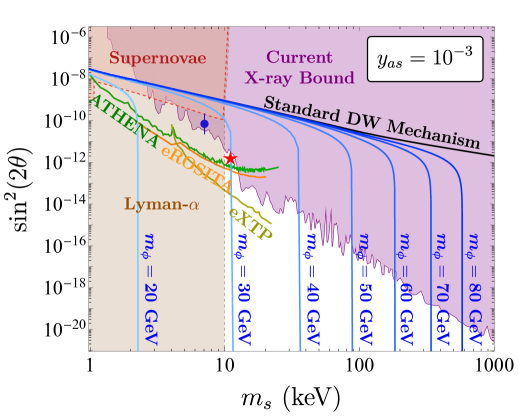
Figure 1: Sterile neutrino mass versus mixing angle for a fixed active-sterile neutrino coupling $y_{as}=10^{-3}$. Shaded regions indicate astrophysical constraints, while the open curves on left are future $X$-ray sensitivities. The blue contours satisfy the relic abundance $\Omega_{s}h^{2}=0.12$ for different values of the mediator mass $m_{\phi}$. The black line corresponds to the correct relic density using the DW mechanism. The red star marks a benchmark point (BP) used later to illustrate the yield behavior. The blue point corresponds to the purported 3.5 keV $X$-ray line signal.

A possible alternative to the DW mechanism is the Shi-Fuller mechanism [27], in which a primordial lepton asymmetry ($\eta_{L}\sim 10^{-3}\text{ to }10^{-1}$) resonantly enhances the sterile neutrino production. However, the required lepton asymmetry is several orders of magnitude larger than the observed baryon asymmetry ($\eta_{B}\sim 10^{-10}$) to yield efficient DM production, challenging its consistency with standard cosmology and Big Bang Nucleosynthesis (BBN) [28, 29, 30], although flavor-specific lepton asymmetries can mitigate the BBN bounds [31].

These challenges motivate the need for alternative sterile neutrino DM production mechanisms using non-standard interactions (NSI) in the neutrino sector [32]. Prior studies have explored the effect of self-interactions between the active neutrinos ($\nu_{a}-\nu_{a}$) [33, 34, 35, 36] or between the sterile neutrinos ($\nu_{s}-\nu_{s}$) [37, 38, 39] on the DM production. In this paper, we explore an intriguing new possibility, i.e. NSI between active and sterile neutrinos ($\nu_{a}-\nu_{s}$). While active-sterile NSI has been previously explored in the contexts of BBN [40] and high-energy neutrinos [41, 42], its role in sterile neutrino DM production has not been studied before.

As summarized in Fig. 1, it leads to uniquely new features, very different from the active-active and sterile-sterile self-interaction scenarios. In particular, the active-sterile NSI introduces new number-changing processes, such as $\nu_{a}\nu_{a}\leftrightarrow\nu_{s}\nu_{s}$, providing an efficient sterile neutrino production channel that differs fundamentally from the DW mechanism, as it does not rely on active-sterile mixing. As a result, it extends the accessible parameter space to arbitrarily small mixing angles. It improves upon earlier self-interaction-based production scenarios, which necessarily depend on the mixing angle and underproduce sterile neutrinos below a threshold mixing angle. Additionally, unlike scenarios involving sterile self-interactions, this mechanism does not rely on any fine-tuned resonance to achieve efficient DM production.

Model.— We consider a keV-scale Majorana sterile neutrino, which mixes with active neutrinos with strength $\theta$ and also participates in NSI via a complex scalar mediator, assumed to have mass $m_{\phi}\gtrsim\mathcal{O}(\mathrm{GeV})$. The relevant effective interaction Lagrangian is given by

$$-\mathcal{L}\supset y_{as}\bar{\nu}_{a}\nu_{s}\phi+{\rm h.c.}\,,$$ (1)

where we have taken the coupling constant $y_{as}$ to be real. We have also suppressed the active neutrino flavor index, as the DM production happens above the neutrino decoupling and all flavors lead to qualitatively similar results, although some of the observational constraints are flavor-dependent. A concrete ultraviolet completion of the effective Lagrangian (1) in terms of a CP-conserving two-Higgs-doublet model plus a complex scalar singlet can be found in Ref. [43]. Note that the $\phi$ field does not acquire a vacuum expectation value, and therefore, there is no induced active-sterile neutrino mixing due to the interaction (1).

We assume no primordial population of sterile neutrinos, which are instead produced entirely from the active sector. For a GeV-scale scalar mediator, the decay rate of $\phi\to\nu_{a}\nu_{s}$ is much faster than the relevant production timescales at $\mathcal{O}({\rm MeV})$, provided the coupling satisfies $y_{as}\gtrsim 10^{-8}$. Under this condition, the evolution of the mediator $\phi$ can be safely neglected.

Since sterile neutrinos are not in thermal equilibrium with the active sector, we model their distribution using a Fermi–Dirac (FD) form:

$$f_{s}(p)=\frac{\alpha}{e^{p/T_{s}}+1}\,,$$ (2)

where $p$ is the magnitude of the 3-momentum, $T_{s}$ is an effective temperature and $0<\alpha\lesssim 1$ is a normalization factor encoding the departure from thermal equilibrium. This ansatz approximates the effect of a small chemical potential $\mu_{s}$, while retaining the spectral shape of the FD distribution. Both $T_{s}$ and $\alpha$ are treated as functions of the SM temperature $T$. This form is valid in the dilute regime $f_{s}(p)\ll 1$, where quantum statistical effects are negligible and the distribution approaches the Maxwell–Boltzmann limit. It also recovers the fully thermalized case ($\alpha=1,T_{s}=T$) in the presence of strong coupling.

The new NSI (1) opens up additional channels for active-sterile neutrino scattering (see Figs. 2, 2) and introduces new contributions to the neutrino self-energy (see Figs. 2, 2). It also enables a number-changing process, $\nu_{a}\nu_{a}\to\nu_{s}\nu_{s}$ (see Fig. 2), which plays a central role in the production of sterile neutrinos. Unlike the DW mechanism, this does not rely on active–sterile mixing and can remain efficient even when mixing angles vanish. These reactions are especially important at high temperatures, when production from mixing is negligible.

(a)

(b)

(c)

(d)

(e)

Figure 2: Feynman diagrams illustrating active–sterile NSI contributions to scattering, number-changing interactions, and thermal potentials.

Evolution of Sterile Neutrino DM.— The time-evolution of the sterile neutrino distribution function $f_{s}(p,t)$ can be described by a semi-classical Boltzmann equation derived from the quantum kinetic equation (QKE) [13, 44]. This equation serves as a classical approximation to the full QKE framework, incorporating quantum corrections through an effective active–sterile transition probability. The approximation remains valid in the small mixing angle limit [45, 46, 47].

In the presence of active–sterile NSI, the Boltzmann equation is modified to

$$\frac{\partial f_{s}(t,p)}{\partial t}-Hp\frac{\partial f_{s}(t,p)}{\partial p}=\mathcal{C}_{\nu_{a}\leftrightarrow\nu_{s}}+\mathcal{C}_{\nu_{a}\nu_{a}\leftrightarrow\nu_{s}\nu_{s}},$$ (3)

where $H(t)$ is the Hubble rate. The first collision term on the right-hand side describes sterile neutrino production via active–sterile oscillations. It depends on both the total interaction rate $\Gamma_{\rm tot}=\Gamma_{\mathrm{SM}}+\Gamma_{\mathrm{NSI}}$ and effective potential $\mathcal{V}_{\mathrm{tot}}=\mathcal{V}_{\rm SM}+\mathcal{V}_{\mathrm{NSI}}$, which include contributions from the SM as well as NSI. The second collision term accounts for number-changing interactions induced by NSI; see Supplemental Material.

The SM contribution to the thermally averaged scattering rate of $\nu_{a}$, arising from interactions with charged leptons, is given by [44, 25]

$$\Gamma_{\mathrm{SM}}(p)=C_{a}(T)\,G_{F}^{2}\,p\,T^{4}\,,$$ (4)

where $G_{F}$ the Fermi constant and $C_{a}(T)$ is a temperature-dependent function defined in Refs. [44, 25, 48]. The quantity $\Gamma_{\mathrm{NSI}}$ denotes the interaction rate arising from additional scattering channels induced by NSI. In this scenario, the only relevant process is $\nu_{a}\nu_{s}\leftrightarrow\nu_{a}\nu_{s}$, which contributes to the interaction rates of both active and sterile neutrinos. Specifically, this rate is given by the sum

$$\Gamma_{\mathrm{NSI}}=\Gamma_{\nu_{a}\nu_{s}\leftrightarrow\nu_{a}\nu_{s}}^{(a)}+\Gamma_{\nu_{a}\nu_{s}\leftrightarrow\nu_{a}\nu_{s}}^{(s)}\,.$$ (5)

In the limit of a heavy mediator, these rates simplify to (see Supplemental Material for the derivation)

$$\Gamma_{\nu_{a}\nu_{s}\leftrightarrow\nu_{a}\nu_{s}}^{(i)}(p)\simeq\frac{7\pi y_{as}^{4}}{108\,m_{\phi}^{4}}\,p\,\times\begin{cases}\alpha T_{s}^{4}&\text{for }i=a\\ T^{4}&\text{for }i=s\end{cases}\,.$$ (6)

The SM effective potential can be expressed as [49, 50, 51]

$$\mathcal{V}_{\rm SM}(p)=\ \frac{2\sqrt{2}\zeta(3)\,G_{F}\,\eta_{B}\,T^{3}}{4\pi^{2}}-\frac{8\sqrt{2}\,G_{F}\,p}{3m_{Z}^{2}}\left(\rho_{\nu_{a}}+\rho_{\bar{\nu}_{a}}\right)$$

$$-\frac{8\sqrt{2}\,G_{F}\,p}{3m_{W}^{2}}\left(\rho_{a}+\rho_{\bar{a}}\right)\,,$$ (7)

where the first term is the baryonic contribution and the rest are the thermal contributions, with $\rho_{a},\rho_{\nu_{a}}$ being the energy densities of charged leptons and active neutrinos, respectively. The NSI contribution to the thermal potential arises from the self-energy diagrams shown in Fig. 2 and Fig. 2, and is given by the difference between the active and sterile neutrino effective potentials [52, 39]:

$$\mathcal{V}_{\mathrm{NSI}}=\mathcal{V}_{a}-\mathcal{V}_{s}.$$ (8)

Assuming the sterile neutrino mass is negligible compared to the relevant temperatures, and neglecting thermal corrections from the scalar mediator, the thermal potential for a neutrino species $\nu_{i}$ (with $i=a$ or $s$) induced by the other species $\nu_{j}$ (with $j\neq i$) in the heavy-mediator limit $m_{\phi}^{2}\gg pT$ takes the form [39]

$$\mathcal{V}_{i}(p)\simeq-\frac{7\pi^{2}\,y_{as}^{2}\,}{45\,m_{\phi}^{4}}p\,\times\begin{cases}\alpha T_{s}^{4}&\text{for }i=a\\ T^{4}&\text{for }i=s\end{cases}\,.$$ (9)

In our framework, sterile neutrinos can also be produced directly via the number-changing process $\nu_{a}\nu_{a}\to\nu_{s}\nu_{s}$, as shown in Fig. 2. This contribution is captured by the second collision term in Eq. (3). At early times, when production from the modified DW mechanism is negligible, these interactions play a crucial role in initiating the sterile neutrino population and driving DM production. For a heavy mediator, the corresponding rates simplify to (see Supplemental Material for details)

$$\Gamma_{\nu_{i}\nu_{i}\rightarrow\nu_{j}\nu_{j}}(p)\simeq\frac{7\pi y_{as}^{4}\,}{1440\,m_{\phi}^{4}}p\times\begin{cases}T^{4}&\text{for }i=a,\;j=s\\ \alpha T_{s}^{4}&\text{for }i=s,\;j=a\end{cases}\,.$$ (10)

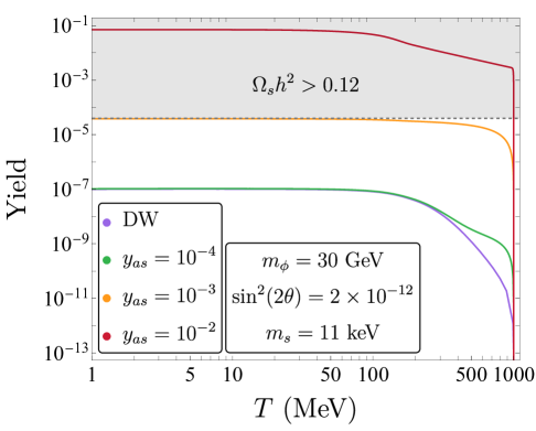
Figure 3: Evolution of the comoving yield for sterile neutrino DM production for the chosen BP as a function of the SM temperature $T$.

We solve the Boltzmann equation (3) by first rewriting it in terms of the evolution equations for the comoving number density $n_{s}$ and energy density $\rho_{s}$ of sterile neutrinos. These quantities are then solved numerically from an initial temperature of 1 GeV up to the active neutrino decoupling temperature, $T\approx 1\,\mathrm{MeV}$. In Fig. 3, we show the evolution of the sterile neutrino comoving yield for a representative benchmark point (BP) with $m_{s}=11\,\text{keV},\sin^{2}2\theta=2\times 10^{-12},m_{\phi}=30\,\text{GeV}$, shown by the red star in Fig. 1, which satisfies current astrophysical constraints and lies within the projected reach of future X-ray telescopes. We notice the following features: (i) For very small couplings (e.g., $y_{as}\lesssim 10^{-4}$), number-changing interactions are only briefly active and quickly become inefficient. In this regime, modifications to the DW mechanism from the additional scatterings and thermal potentials are negligible, and the yield closely tracks the DW baseline. (ii) For slightly larger couplings (e.g., $y_{as}=10^{-3}$), number-changing processes remain efficient for a longer duration, sustaining production down to $T\sim 100\,\mathrm{MeV}$. As a result, the yield exceeds the DW curve before freezing in. After number-changing production ceases, the spectrum gradually returns to a DW-like shape. (iii) For large couplings (e.g., $y_{as}=10^{-2}$), number-changing interactions remain efficient throughout the entire production window, keeping the sterile sector in thermal contact with the active neutrinos. The yield quickly rises to the overproduction region, well above the DW line. This scenario is cosmologically excluded as it would indicate overproduction of DM as well as extra number of relativistic degrees of freedom at BBN.

Note that the final relic abundance is determined by the suppression factor $\alpha$ in Eq. (2) while the effective temperature $T_{s}$ controls the spectral shape of the sterile neutrino population. The evolution of these quantities are given in the Supplemental Material

Results and Discussion.— Figure 1 presents the viable parameter space in the plane of sterile neutrino mass and active–sterile mixing angle for a fixed value of $y_{as}=10^{-3}$. We find that the presence of NSI significantly enlarges the allowed region beyond the traditional DW scenario. In particular, viable production can now happen at much smaller mixing angles and even remains efficient in the limit of vanishing mixing. This behavior differs substantially from both the standard DW mechanism and earlier works on both active and sterile neutrino self-interaction scenarios [33, 34, 36, 38, 37, 39], where underproduction necessarily occurs at small mixing due to the lack of efficient production channels.

Moreover, in the previously discussed active-active and sterile-sterile NSI scenarios, for heavy mediators, a substantial departure from DW typically requires couplings $\gtrsim 10^{-2}$ [39, 33]. However in our case, such large couplings lead to overproduction of sterile neutrinos. In fact, efficient production can be achieved at smaller couplings without relying on active–sterile mixing. Figure 1 indicates a transition in the parameter space: for a given coupling and mediator mass, there exists a minimum sterile neutrino mass above which number-changing interactions alone can generate the observed relic abundance irrespective of the mixing angle. As the mediator mass increases, resulting abundance approaches that of the standard DW scenario, as expected in the heavy mediator regime.

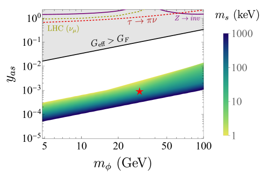
Figure 4: Mediator mass versus coupling strength for allowed values of mixing angle. The colored band denotes the region with the correct DM abundance ($\Omega_{s}h^{2}=0.12$). Grey shaded region corresponds to parameters where $G_{\rm eff}>G_{F}$. The laboratory constraints shown here are all within the cosmologically disfavored regime. The red star corresponds to the BP used in Fig. 3.

The viable parameter space now extends into regions where sterile neutrino DM can be produced efficiently without violating existing astrophysical constraints from X-ray telescopes such as Chandra [53], XMM-Newton [54], NuSTAR [17], and XRISM [55] and at higher energies from gamma-ray telescopes like INTEGRAL/SPI [56]. We also include projected sensitivities from future missions such as ATHENA [57], eROSITA [58], and eXTP [59]. The presence of sterile neutrinos can also influence the evolution of core-collapse supernovae, leading to constraints on their mass and mixing angle [60, 61, 62]. The supernova constraint shown in Fig. 1 specifically applies to $\nu_{e}-\nu_{s}$ mixing [60]. In addition, Lyman-$\alpha$ forest measurements impose a lower bound on the warm DM mass, which corresponds to a present-day root-mean-square velocity of $v_{\text{rms},\,\text{today}}\lesssim 16\,\text{m/s}$ [63]. From this, we can infer that the sterile neutrino mass should satisfy a lower bound of approximately $m_{s}\gtrsim 10\,\text{keV}$. The blue circle in Fig. 1 represents the reported detection of an unidentified $X$-ray line near 3.5 keV [64, 65, 66] which would correspond to a 7.1 keV sterile neutrino, although the existence of the 3.5 keV line signal remains debatable [67].

Fig. 4 shows the allowed parameter space in the plane of mediator mass $m_{\phi}$ and coupling $y_{as}$, assuming sterile neutrino production is dominated by NSI. We find that the result holds for any mixing angle allowed by astrophysical bounds. We find that sterile neutrinos with masses in the range 1–100 keV can account for the observed relic abundance, $\Omega_{s}h^{2}=0.12$, even in the absence of mixing, for couplings of order $y_{as}\sim 10^{-4}$. At smaller couplings ($y_{as}\lesssim 5\times 10^{-5}$), the number-changing process $\nu_{a}\nu_{a}\rightarrow\nu_{s}\nu_{s}$ becomes inefficient, and the combined effect of scattering and oscillations is insufficient to generate the observed relic abundance. The range of couplings considered in our analysis remains consistent with current experimental constraints. For larger values ($y_{as}\gtrsim 10^{-3}$), sterile neutrinos are typically overproduced unless the mediator is sufficiently heavy to suppress the production rate. The gray shaded regions in Fig. 4 indicate parameter choices where the effective neutrino coupling $G_{\rm eff}\equiv y_{as}^{2}/m_{\phi}^{2}$ is greater than $G_{F}$ and is therefore cosmologically excluded, because it would hinder neutrino coupling at MeV-scale. Notably, we find that experimental bounds from $Z\rightarrow\text{invisible}$ decays, tau decays and LHC searches [68, 69] are already encompassed within the cosmologically disfavored region.

The lower bound of $\sim 5\leavevmode\nobreak\ \mathrm{GeV}$ in Fig. 4 reflects the regime where the mediator mass approaches the temperature at which sterile neutrinos are produced. Below this scale, the mediator can become kinematically accessible in the thermal bath during production, potentially modifying the sterile sector’s evolution and enabling additional scattering processes involving on-shell $\phi$ exchange. A detailed treatment of this light mediator regime is left for future work.

Acknowledgments.— We thank Maria Dias Astros and Stefan Vogl for useful discussion on Ref. [39]. We also thank the organizers of ‘Particle Physics on the Plains’ (PPP) 2023 at University of Kansas, where this work was initiated. The work of PSBD, JT and AUR was partly supported by the U.S. Department of Energy under grant No. DE-SC0017987. PSBD was also partly supported by a Humboldt Fellowship from the Alexander von Humboldt Foundation. The work of BD is supported by the U.S. DOE Grant DE-SC0010813. SG acknowledges the J.C. Bose Fellowship (JCB/2020/000011) by the Anusandhan National Research Foundation, and Department of Space, Govt. of India. She also acknowledges Northwestern University (NU), where a part of this work was done, for hospitality and Fullbright-Nehru Academic and Professional Excellence fellowship for funding the visit to NU.

Supplemental Material

.1 A. Collision terms

The collision terms appearing in the Boltzmann equation (3) are given explicitly below:

$$\mathcal{C}_{\nu_{a}\leftrightarrow\nu_{s}}(p)= \frac{\Gamma_{\rm tot}}{4}\frac{\omega^{2}(p)\sin^{2}(2\theta)}{\omega^{2}(p)\sin^{2}(2\theta)+D^{2}(p)+[\omega(p)\cos(2\theta)-\mathcal{V}_{\mathrm{tot}}]^{2}}\left[f_{a}(t,p)-f_{s}(t,p)\right]\,.$$ (11)

$$\mathcal{C}_{\nu_{a}\nu_{a}\leftrightarrow\nu_{s}\nu_{s}}(p)= \frac{1}{2E}\int\prod_{i=1}^{3}d\Pi_{i}\,(2\pi)^{4}\delta^{(4)}(\mathbf{P}_{1}+\mathbf{P}_{2}-\mathbf{P}_{3}-\mathbf{P})\big{(}\,|\mathcal{M}_{\nu_{a}\nu_{a}\rightarrow\nu_{s}\nu_{s}}|^{2}f_{a}(p_{1})\,f_{a}(p_{2})\,[1\mp f_{s}(p_{3})]\,[1\mp f_{s}(p)]$$

$$\qquad\qquad-|\mathcal{M}_{\nu_{s}\nu_{s}\rightarrow\nu_{a}\nu_{a}}|^{2}f_{s}(p_{3})\,f_{s}(p)\,[1\mp f_{a}(p_{1})]\,[1\mp f_{a}(p_{2})]\,\big{)}\,.$$ (12)

Here, $\mathrm{d}\Pi_{i}$ denote the Lorentz-invariant phase space elements, the boldface $\mathbf{P}_{i}$’s are the 4-momenta, $p_{i}$’s are the magnitudes of the 3-momenta, and $\omega(p)\approx\frac{m_{s}^{2}}{2p}$ is the vacuum oscillation frequency for $m_{s}\gg m_{\nu_{a}}$. The total interaction rate $\Gamma_{\rm tot}=\Gamma_{\mathrm{SM}}+\Gamma_{\mathrm{NSI}}$ and effective potential $\mathcal{V}_{\mathrm{tot}}=\mathcal{V}_{\rm SM}+\mathcal{V}_{\mathrm{NSI}}$ incorporate both the SM contributions and modifications from NSI. The term $D(p)=\Gamma_{\rm tot}/2$ corresponds to the quantum damping rate, which accounts for decoherence effects in neutrino propagation.

The resonance condition for modified DW production is given by

$$\omega(p)\cos(2\theta)-\mathcal{V}_{\mathrm{tot}}=0,$$ (13)

which yields two distinct resonance scenarios: a standard MSW-like resonance when $\omega(p)\cos(2\theta)=\mathcal{V}_{\mathrm{tot}}$, and a second case where the total effective potential vanishes, $\mathcal{V}_{\mathrm{tot}}=0$. These conditions typically require large couplings of order $y_{as}\sim\mathcal{O}(10^{-2})$ or higher, which would lead to excessive production of sterile neutrinos through number-changing processes present in our NSI framework. For this reason, we do not consider resonance effects in this work.

We can simplify Eq. (.1) by noting that $|\mathcal{M}_{\nu_{s}\nu_{s}\rightarrow\nu_{a}\nu_{a}}|^{2}=|\mathcal{M}_{\nu_{a}\nu_{a}\rightarrow\nu_{s}\nu_{s}}|^{2}\equiv|\mathcal{M}|^{2}$, and neglecting Pauli blocking and Bose enhancement effects (i.e., $1\mp f\approx 1$). Under these assumptions, the collision term reduces to:

$$\mathcal{C}_{\nu_{a}\nu_{a}\leftrightarrow\nu_{s}\nu_{s}}(p)=\frac{1}{2E}\int\prod_{i=1}^{3}d\Pi_{i}\,(2\pi)^{4}\delta^{(4)}(\mathbf{P}_{1}+\mathbf{P}_{2}-\mathbf{P}_{3}-\mathbf{P})\,|\mathcal{M}|^{2}\left[f_{a}(p_{1})f_{a}(p_{2})-f_{s}(p_{3})f_{s}(p)\right].$$ (14)

The zeroth and first moments of Eqs. (11, .1):

$$\mathrm{C}_{n_{s}}=\int\frac{d^{3}p}{(2\pi)^{3}}\,\big{(}\mathcal{C}_{\nu_{a}\leftrightarrow\nu_{s}}(p)+\mathcal{C}_{\nu_{a}\nu_{a}\leftrightarrow\nu_{s}\nu_{s}}(p)\big{)},\qquad\mathrm{C}_{\rho_{s}}=\int\frac{d^{3}p}{(2\pi)^{3}}\,p\,\big{(}\mathcal{C}_{\nu_{a}\leftrightarrow\nu_{s}}(p)+\mathcal{C}_{\nu_{a}\nu_{a}\leftrightarrow\nu_{s}\nu_{s}}(p)\big{)},$$ (15)

enter the integrated Boltzmann equations governing the evolution of the sterile neutrino number and energy densities:

$$\dot{n}_{s}+3Hn_{s}=\mathrm{C}_{n_{s}},\qquad\dot{\rho}_{s}+4H\rho_{s}=\mathrm{C}_{\rho_{s}}.$$ (16)

The contribution from the number-changing process $\nu_{a}\nu_{a}\leftrightarrow\nu_{s}\nu_{s}$ can be recast in terms of interaction rate as

$$\mathrm{C}_{\nu_{a}\nu_{a}\leftrightarrow\nu_{s}\nu_{s}}^{(n)}= \int\frac{d^{3}p}{(2\pi)^{3}}\,\mathcal{C}_{\nu_{a}\nu_{a}\leftrightarrow\nu_{s}\nu_{s}}(p)=\int d\Pi\big{(}f_{a}(p)\,\Gamma_{\nu_{a}\nu_{a}\rightarrow\nu_{s}\nu_{s}}(p)-f_{s}(p)\,\Gamma_{\nu_{s}\nu_{s}\rightarrow\nu_{a}\nu_{a}}(p)\big{)},$$

$$\mathrm{C}_{\nu_{a}\nu_{a}\leftrightarrow\nu_{s}\nu_{s}}^{(\rho)}= \int\frac{d^{3}p}{(2\pi)^{3}}\,p\,\mathcal{C}_{\nu_{a}\nu_{a}\leftrightarrow\nu_{s}\nu_{s}}(p)=\int d\Pi\,p\big{(}f_{a}(p)\,\Gamma_{\nu_{a}\nu_{a}\rightarrow\nu_{s}\nu_{s}}(p)-f_{s}(p)\,\Gamma_{\nu_{s}\nu_{s}\rightarrow\nu_{a}\nu_{a}}(p)\big{)}\,.$$ (17)

.2 B. Interaction rates

The general form for the interaction rate of a neutrino species $\nu_{i}$ in a bath of $\nu_{j}$ is

$$\Gamma_{\nu_{i}\nu_{j}\,\leftrightarrow\,{\rm final}}^{(i)}(p)=\int\frac{\mathrm{d}^{3}k}{8\pi^{3}}\,v_{\text{M\o ller}}\,f_{j}(k)\,\sigma_{ij\,\leftrightarrow\,{\rm final}}(p,k),$$ (18)

where the Møller velocity between the incident and target neutrinos is defined as [70]

$$v_{\text{Møller}}=\sqrt{\left(\vec{v}_{\rm in}-\vec{v}_{\rm tar}\right)^{2}-(\vec{v}_{\rm in}\times\vec{v}_{\rm tar})^{2}},$$

and $\sigma_{\nu_{i}\nu_{j}\leftrightarrow\text{final}}$ is the corresponding scattering cross section. In the ultra-relativistic limit, this simplifies to $v_{\text{M\o ller}}=1-\cos\theta$, where $\theta$ is the angle between incoming and target momenta. The rate then becomes

$$\Gamma_{\nu_{i}\nu_{j}\leftrightarrow\text{final}}^{(i)}(p)=\frac{1}{16\pi^{2}p^{2}}\int_{0}^{\infty}\mathrm{d}k\,f_{j}(k)\int_{0}^{4pk}\mathrm{d}s\,s\,\sigma_{\nu_{i}\nu_{j}\rightarrow\text{final}}(s),$$ (19)

with $s=2pk(1-\cos\theta)$ the Mandelstam variable.

The distribution functions for the active and sterile neutrino species are taken to be

$$f_{a}(p)=\frac{1}{e^{p/T}+1},\quad f_{s}(p)=\frac{\alpha}{e^{p/T_{s}}+1},$$

as explained in the main text.

For the process $\nu_{a}\nu_{s}\rightarrow\nu_{a}\nu_{s}$, both $s$-channel and $u$-channel diagrams contribute. The total spin-averaged squared matrix element is given by

$$\overline{|\mathcal{M}|^{2}}_{\nu_{a}\nu_{s}\rightarrow\nu_{a}\nu_{s}}=\frac{16y_{as}^{4}\left(m_{\phi}^{4}(s^{2}+st+t^{2})+m_{\phi}^{2}\left(\Gamma_{\phi}^{2}(s^{2}+st+t^{2})-3st(s+t)\right)+3s^{2}(s+t)^{2}\right)}{(\Gamma_{\phi}^{2}m_{\phi}^{2}+(m_{\phi}^{2}-s)^{2})(\Gamma_{\phi}^{2}m_{\phi}^{2}+(m_{\phi}^{2}+s+t)^{2})}\,,$$ (20)

where $\Gamma_{\phi}=\frac{y_{as}^{2}}{4\pi}m_{\phi}$ is the decay width of the scalar mediator $\phi$. The corresponding cross section is:

$$\sigma_{\nu_{a}\nu_{s}\rightarrow\nu_{a}\nu_{s}}(s) =\frac{y_{as}^{4}}{\pi s^{2}\left(\Gamma_{\phi}^{2}m_{\phi}^{2}+(m_{\phi}^{2}-s)^{2}\right)}\Bigg{[}\left(2m_{\phi}^{2}-3s\right)m_{\phi}^{2}(m_{\phi}^{2}-s)\log\left(\frac{m_{\phi}^{2}}{m_{\phi}^{2}+s}\right)+\frac{s\left(2m_{\phi}^{6}-4m_{\phi}^{4}s+m_{\phi}^{2}s^{2}+3s^{3}\right)}{m_{\phi}^{2}+s}\Bigg{]}.$$ (21)

The rate expressions simplify in the following limits:

$$\Gamma_{\nu_{a}\nu_{s}\leftrightarrow\nu_{a}\nu_{s}}^{(s)}(p)\approx\begin{cases}\displaystyle\frac{7\pi y^{4}\,pT^{4}}{108\,m_{\phi}^{4}}&\text{for }pT\ll m_{\phi}^{2}\\[6.45831pt] \displaystyle\frac{y^{4}T^{2}}{16\pi\,p}&\text{for }pT\gg m_{\phi}^{2}\end{cases}\quad;\quad\Gamma_{\nu_{a}\nu_{s}\leftrightarrow\nu_{a}\nu_{s}}^{(a)}(p)\approx\begin{cases}\displaystyle\frac{7\pi\alpha y^{4}\,pT_{s}^{4}}{108\,m_{\phi}^{4}}&\text{for }pT_{s}\ll m_{\phi}^{2}\\[6.45831pt] \displaystyle\frac{\alpha y^{4}T_{s}^{2}}{16\pi\,p}&\text{for }pT_{s}\gg m_{\phi}^{2}\end{cases}.$$ (22)

For the process $\nu_{a}\nu_{a}\leftrightarrow\nu_{s}\nu_{s}$, both $t$-channel and $u$-channel diagrams contribute. The total spin-averaged squared matrix element is given by:

$$\left|\mathcal{M}_{\nu_{a}\nu_{a}\leftrightarrow\nu_{s}\nu_{s}}\right|^{2} =\frac{64y^{4}\left(m_{\phi}^{4}\left(s^{2}+3st+3t^{2}\right)+m_{\phi}^{2}\left(s^{2}\left(\Gamma_{\phi}^{2}-t\right)-st\left(t-3\Gamma_{\phi}^{2}\right)+3\Gamma_{\phi}^{2}t^{2}\right)+t^{2}(s+t)^{2}\right)}{\left(\Gamma_{\phi}^{2}m_{\phi}^{2}+\left(m_{\phi}^{2}-t\right)^{2}\right)\left(\Gamma_{\phi}^{2}m_{\phi}^{2}+\left(m_{\phi}^{2}+s+t\right)^{2}\right)}\,.$$ (23)

Assuming the narrow width limit $\Gamma_{\phi}\rightarrow 0$ and negligible neutrino masses $m_{s},\,m_{\nu_{a}}\ll\sqrt{s}$, the total cross section simplifies to:

$$\sigma_{\nu_{a}\nu_{a}\leftrightarrow\nu_{s}\nu_{s}}(s)=\frac{2y^{4}\left(3\,m_{\phi}^{2}+s\right)}{\pi s^{2}}\left[\frac{s}{m_{\phi}^{2}+s}+\frac{2\,m_{\phi}^{2}}{\left(2\,m_{\phi}^{2}+s\right)}\log\left(\frac{m_{\phi}^{2}}{m_{\phi}^{2}+s}\right)\right].$$ (24)

In the limiting cases, the corresponding rates become

$$\Gamma_{\nu_{a}\nu_{a}\rightarrow\nu_{s}\nu_{s}}(p)\approx\begin{cases}\displaystyle\frac{7\pi y^{4}\,pT^{4}}{1440\,m_{\phi}^{4}}&\text{for }pT\ll m_{\phi}^{2}\\[6.45831pt] \displaystyle\frac{y^{4}\,T^{2}}{384\pi\,p}&\text{for }pT\gg m_{\phi}^{2}\end{cases}\quad;\quad\Gamma_{\nu_{s}\nu_{s}\rightarrow\nu_{a}\nu_{a}}(p)\approx\begin{cases}\displaystyle\frac{7\pi y^{4}\,pT_{s}^{4}}{1440\,m_{\phi}^{4}}&\text{for }pT_{s}\ll m_{\phi}^{2}\\[6.45831pt] \displaystyle\frac{y^{4}\,T_{s}^{2}}{384\pi\,p}&\text{for }pT_{s}\gg m_{\phi}^{2}\end{cases}.$$ (25)

.3 C. Evolution of $\alpha$ and $T_{s}$

Figure 5 shows the evolution of the suppression factor $\alpha$ and the effective temperature $T_{s}$ with the SM temperature. From the right panel, it can be seen that for very small couplings (e.g., $y_{as}\lesssim 10^{-4}$) the suppression factor remains small: $\alpha\ll 1$, resulting in an under-abundance of DM. For slightly larger couplings (e.g., $y_{as}=10^{-3}$), $\alpha$ is higher as compared to the lower-coupling case, ensuring the correct relic abundance observed in Fig. 3. For even larger couplings (e.g., $y_{as}=10^{-2}$), $\alpha\sim 0.01\text{ to }1$ and $T_{s}\gtrsim T$, signaling (near-)full thermalization of the sterile population leading to an over-abundance as was seen in Fig. 3. Note that in all cases, the extra interaction causes the effective temperature $T_{s}$ to be initially higher than the DW value, but it gradually converges to the DW case at lower temperatures for smaller Yukawa couplings, while for large Yuakwa couplings, $T_{s}$ remains larger than $T$ implying that the sterile neutrino enters the thermal bath, which is therefore disfavored. The variation in $T_{s}$ across the parameter space, however, is modest in all cases considered. Together, the parameters $\alpha$ and $T_{s}$ provide a complete characterization of sterile neutrino DM production in this framework.

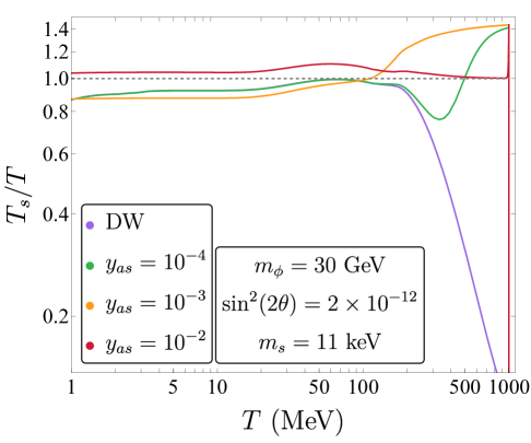
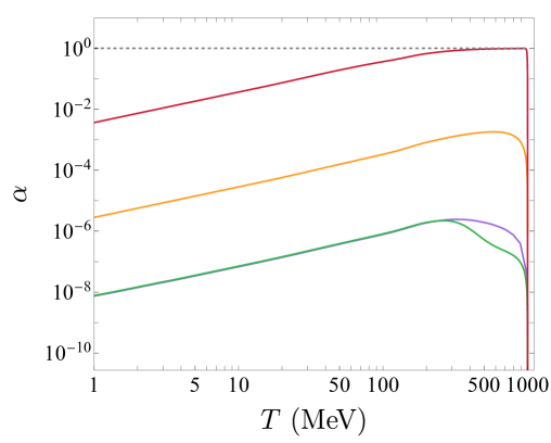
Figure 5: Evolution of the sterile neutrino distribution parameters $T_{s}$ and $\alpha$ for the BP ($m_{s}=11\,\mathrm{keV}$, $\sin^{2}2\theta=2\times 10^{-12}$, $m_{\phi}=30\,\mathrm{GeV}$) as functions of the photon temperature $T$.

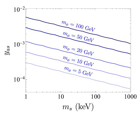
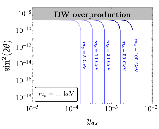
Figure 6: Left: Sterile neutrino mass vs. coupling strength parameter space for active-sterile mixing angle $\sin^{2}2\theta=0$. Blue contour lines indicate where the relic abundance satisfies $\Omega_{s}h^{2}=0.12$. Right: Parameter space of mixing angle versus coupling strength for a 11 keV sterile neutrino. Contours show values of $\Omega_{s}h^{2}=0.12$ for different mediator masses. The gray shaded region indicates where the DW mechanism alone leads to overproduction.

.4 D. Additional plots of the parameter space

Figure 6 provides complementary information to what has been shown in Figs. 1 and 4. The left panel of Fig. 6 left panel shows the variation of $y_{as}$ as a function of $m_{s}$ for different values of $m_{\phi}$ and for vanishing mixing angle. The correct relic density of $\nu_{s}$ is produced along the blue contours. We see that for larger (smaller) values of the mediator mass, we require larger (smaller) values of the Yukawa coupling to get the correct relic density.

The right panel of Fig. 6 shows the variation of $\sin^{2}(2\theta)$ as a function of $y_{as}$ for different values of $m_{\phi}$ and for a fixed DM mass of 11 keV. As in the left panel, the correct relic density is obtained along the blue contours. We see that depending on the mediator mass, the DM production is dominantly governed by the Yukawa coupling, irrespective of the mixing angle. But as the Yukawa coupling becomes small, we approach the DW limit, where the DM production is governed by the mixing angle. The grey shaded region on the top corresponds to large mixing angles for which even the DW mechanism leads to DM overproduction.

References

- Arcadi et al. [2025] G. Arcadi, D. Cabo-Almeida, M. Dutra, P. Ghosh, M. Lindner, Y. Mambrini, J. P. Neto, M. Pierre, S. Profumo, and F. S. Queiroz, Eur. Phys. J. C 85, 152 (2025), arXiv:2403.15860 [hep-ph] .
- Baer et al. [2015] H. Baer, K.-Y. Choi, J. E. Kim, and L. Roszkowski, Phys. Rept. 555, 1 (2015), arXiv:1407.0017 [hep-ph] .
- Feng and Kumar [2008] J. L. Feng and J. Kumar, Phys. Rev. Lett. 101, 231301 (2008), arXiv:0803.4196 [hep-ph] .
- Hall et al. [2010] L. J. Hall, K. Jedamzik, J. March-Russell, and S. M. West, JHEP 03, 080, arXiv:0911.1120 [hep-ph] .
- Adams et al. [2022] C. B. Adams et al., in Snowmass 2021 (2022) arXiv:2203.14923 [hep-ex] .
- Abazajian [2017] K. N. Abazajian, Phys. Rept. , 1 (2017), arXiv:1705.01837 [hep-ph] .
- Hui [2021] L. Hui, Ann. Rev. Astron. Astrophys. 59, 247 (2021), arXiv:2101.11735 [astro-ph.CO] .
- Bird et al. [2023] S. Bird et al., Phys. Dark Univ. 41, 101231 (2023), arXiv:2203.08967 [hep-ph] .
- Asaka et al. [2005] T. Asaka, S. Blanchet, and M. Shaposhnikov, Phys. Lett. B 631, 151 (2005), arXiv:hep-ph/0503065 .
- Drewes et al. [2017] M. Drewes et al., JCAP 01, 025, arXiv:1602.04816 [hep-ph] .
- Boyarsky et al. [2019] A. Boyarsky, M. Drewes, T. Lasserre, S. Mertens, and O. Ruchayskiy, Prog. Part. Nucl. Phys. 104, 1 (2019), arXiv:1807.07938 [hep-ph] .
- Dasgupta and Kopp [2021] B. Dasgupta and J. Kopp, Phys. Rept. 928, 1 (2021), arXiv:2106.05913 [hep-ph] .
- Dodelson and Widrow [1994] S. Dodelson and L. M. Widrow, Phys. Rev. Lett. 72, 17 (1994), arXiv:hep-ph/9303287 .
- Riemer-Sørensen [2016] S. Riemer-Sørensen, Astron. Astrophys. 590, A71 (2016), arXiv:1405.7943 [astro-ph.CO] .
- Anderson et al. [2015] M. E. Anderson, E. Churazov, and J. N. Bregman, Mon. Not. Roy. Astron. Soc. 452, 3905 (2015), arXiv:1408.4115 [astro-ph.HE] .
- Dessert et al. [2020] C. Dessert, N. L. Rodd, and B. R. Safdi, Science 367, 1465 (2020), arXiv:1812.06976 [astro-ph.CO] .
- Ng et al. [2019] K. C. Y. Ng, B. M. Roach, K. Perez, J. F. Beacom, S. Horiuchi, R. Krivonos, and D. R. Wik, Phys. Rev. D 99, 083005 (2019), arXiv:1901.01262 [astro-ph.HE] .
- Wang et al. [2017] M.-Y. Wang, J. F. Cherry, S. Horiuchi, and L. E. Strigari, (2017), arXiv:1712.04597 [astro-ph.CO] .
- Nadler et al. [2021] E. O. Nadler et al. (DES), Phys. Rev. Lett. 126, 091101 (2021), arXiv:2008.00022 [astro-ph.CO] .
- Zelko et al. [2022] I. A. Zelko, T. Treu, K. N. Abazajian, D. Gilman, A. J. Benson, S. Birrer, A. M. Nierenberg, and A. Kusenko, Phys. Rev. Lett. 129, 191301 (2022), arXiv:2205.09777 [hep-ph] .
- Newton et al. [2024] O. Newton, M. R. Lovell, C. S. Frenk, A. Jenkins, J. C. Helly, S. Cole, and A. J. Benson, (2024), arXiv:2408.16042 [astro-ph.CO] .
- Tan et al. [2025] C. Y. Tan, A. Dekker, and A. Drlica-Wagner, Phys. Rev. D 111, 063079 (2025), arXiv:2409.18917 [astro-ph.CO] .
- Tremaine and Gunn [1979] S. Tremaine and J. E. Gunn, Phys. Rev. Lett. 42, 407 (1979).
- Boyarsky et al. [2009a] A. Boyarsky, O. Ruchayskiy, and D. Iakubovskyi, JCAP 03, 005, arXiv:0808.3902 [hep-ph] .
- Merle et al. [2016] A. Merle, A. Schneider, and M. Totzauer, JCAP 04, 003, arXiv:1512.05369 [hep-ph] .
- Bezrukov et al. [2024] F. Bezrukov, D. Gorbunov, and E. Koreshkova, (2024), arXiv:2412.20585 [hep-ph] .
- Shi and Fuller [1999] X.-D. Shi and G. M. Fuller, Phys. Rev. Lett. 82, 2832 (1999), arXiv:astro-ph/9810076 .
- Shi et al. [1993] X. Shi, D. N. Schramm, and B. D. Fields, Phys. Rev. D 48, 2563 (1993), arXiv:astro-ph/9307027 .
- Boyarsky et al. [2009b] A. Boyarsky, O. Ruchayskiy, and M. Shaposhnikov, Ann. Rev. Nucl. Part. Sci. 59, 191 (2009b), arXiv:0901.0011 [hep-ph] .
- Bodeker and Klaus [2020] D. Bodeker and A. Klaus, JHEP 07, 218, arXiv:2005.03039 [hep-ph] .
- Gorbunov et al. [2025] D. Gorbunov, D. Kalashnikov, and G. Krugan, (2025), arXiv:2502.17374 [hep-ph] .
- Dev et al. [2019] P. S. B. Dev et al., SciPost Phys. 2, 001 (2019), arXiv:1907.00991 [hep-ph] .
- De Gouvêa et al. [2020] A. De Gouvêa, M. Sen, W. Tangarife, and Y. Zhang, Phys. Rev. Lett. 124, 081802 (2020), arXiv:1910.04901 [hep-ph] .
- Kelly et al. [2020] K. J. Kelly, M. Sen, W. Tangarife, and Y. Zhang, Phys. Rev. D 101, 115031 (2020), arXiv:2005.03681 [hep-ph] .
- Alonso-Álvarez and Cline [2021] G. Alonso-Álvarez and J. M. Cline, JCAP 10, 041, arXiv:2107.07524 [hep-ph] .
- Benso et al. [2022] C. Benso, W. Rodejohann, M. Sen, and A. U. Ramachandran, Phys. Rev. D 105, 055016 (2022), arXiv:2112.00758 [hep-ph] .
- Johns and Fuller [2019] L. Johns and G. M. Fuller, Phys. Rev. D 100, 023533 (2019), arXiv:1903.08296 [hep-ph] .
- Bringmann et al. [2023] T. Bringmann, P. F. Depta, M. Hufnagel, J. Kersten, J. T. Ruderman, and K. Schmidt-Hoberg, Phys. Rev. D 107, L071702 (2023), arXiv:2206.10630 [hep-ph] .
- Astros and Vogl [2024] M. D. Astros and S. Vogl, JHEP 03, 032, arXiv:2307.15565 [hep-ph] .
- Babu and Rothstein [1992] K. S. Babu and I. Z. Rothstein, Phys. Lett. B 275, 112 (1992).
- Fiorillo et al. [2020a] D. F. G. Fiorillo, G. Miele, S. Morisi, and N. Saviano, Phys. Rev. D 101, 083024 (2020a), arXiv:2002.10125 [hep-ph] .
- Fiorillo et al. [2020b] D. F. G. Fiorillo, S. Morisi, G. Miele, and N. Saviano, Phys. Rev. D 102, 083014 (2020b), arXiv:2007.07866 [hep-ph] .
- Dutta et al. [2020] B. Dutta, S. Ghosh, and T. Li, Phys. Rev. D 102, 055017 (2020), arXiv:2006.01319 [hep-ph] .
- Abazajian et al. [2001] K. Abazajian, G. M. Fuller, and M. Patel, Phys. Rev. D 64, 023501 (2001), arXiv:astro-ph/0101524 .
- Bell et al. [1999] N. F. Bell, R. R. Volkas, and Y. Y. Y. Wong, Phys. Rev. D 59, 113001 (1999), arXiv:hep-ph/9809363 .
- Kishimoto and Fuller [2008] C. T. Kishimoto and G. M. Fuller, Phys. Rev. D 78, 023524 (2008), arXiv:0802.3377 [astro-ph] .
- Johns [2019] L. Johns, Phys. Rev. D 100, 083536 (2019), arXiv:1908.04244 [hep-ph] .
- Asaka et al. [2007] T. Asaka, M. Laine, and M. Shaposhnikov, JHEP 01, 091, [Erratum: JHEP 02, 028 (2015)], arXiv:hep-ph/0612182 .
- Nötzold and Raffelt [1988] D. Nötzold and G. Raffelt, Nucl. Phys. B 307, 924 (1988).
- D’Olivo et al. [1992] J. C. D’Olivo, J. F. Nieves, and M. Torres, Phys. Rev. D 46, 1172 (1992).
- Abazajian [2006] K. Abazajian, Phys. Rev. D 73, 063506 (2006), arXiv:astro-ph/0511630 .
- Dasgupta and Kopp [2014] B. Dasgupta and J. Kopp, Phys. Rev. Lett. 112, 031803 (2014), arXiv:1310.6337 [hep-ph] .
- Hofmann et al. [2016] F. Hofmann, J. S. Sanders, K. Nandra, N. Clerc, and M. Gaspari, Astron. Astrophys. 592, A112 (2016), arXiv:1606.04091 [astro-ph.CO] .
- Borriello et al. [2012] E. Borriello, M. Paolillo, G. Miele, G. Longo, and R. Owen, Mon. Not. Roy. Astron. Soc. 425, 1628 (2012), arXiv:1109.5943 [astro-ph.GA] .
- Yin et al. [2025] W. Yin, Y. Fujita, Y. Ezoe, and Y. Ishisaki, (2025), arXiv:2503.04726 [hep-ph] .
- Calore et al. [2023] F. Calore, A. Dekker, P. D. Serpico, and T. Siegert, Mon. Not. Roy. Astron. Soc. 520, 4167 (2023), [Erratum: Mon.Not.Roy.Astron.Soc. 538, 132 (2025)], arXiv:2209.06299 [hep-ph] .
- Barret et al. [2020] D. Barret, A. Decourchelle, A. Fabian, M. Guainazzi, K. Nandra, R. Smith, and J.-W. d. Herder, Astron. Nachr. 341, 224 (2020), arXiv:1912.04615 [astro-ph.IM] .
- Merloni et al. [2012] A. Merloni et al. (eROSITA), (2012), arXiv:1209.3114 [astro-ph.HE] .
- Malyshev et al. [2020] D. Malyshev, C. Thorpe-Morgan, A. Santangelo, J. Jochum, and S.-N. Zhang, Phys. Rev. D 101, 123009 (2020), arXiv:2001.07014 [astro-ph.HE] .
- Shi and Sigl [1994] X. Shi and G. Sigl, Phys. Lett. B 323, 360 (1994), [Erratum: Phys.Lett.B 324, 516–516 (1994)], arXiv:hep-ph/9312247 .
- Raffelt and Zhou [2011] G. G. Raffelt and S. Zhou, Phys. Rev. D 83, 093014 (2011), arXiv:1102.5124 [hep-ph] .
- Argüelles et al. [2019] C. A. Argüelles, V. Brdar, and J. Kopp, Phys. Rev. D 99, 043012 (2019), arXiv:1605.00654 [hep-ph] .
- Garzilli et al. [2021] A. Garzilli, A. Magalich, O. Ruchayskiy, and A. Boyarsky, Mon. Not. Roy. Astron. Soc. 502, 2356 (2021), arXiv:1912.09397 [astro-ph.CO] .
- Boyarsky et al. [2014] A. Boyarsky, O. Ruchayskiy, D. Iakubovskyi, and J. Franse, Phys. Rev. Lett. 113, 251301 (2014), arXiv:1402.4119 [astro-ph.CO] .
- Bulbul et al. [2014] E. Bulbul, M. Markevitch, A. Foster, R. K. Smith, M. Loewenstein, and S. W. Randall, Astrophys. J. 789, 13 (2014), arXiv:1402.2301 [astro-ph.CO] .
- Cappelluti et al. [2018] N. Cappelluti, E. Bulbul, A. Foster, P. Natarajan, M. C. Urry, M. W. Bautz, F. Civano, E. Miller, and R. K. Smith, Astrophys. J. 854, 179 (2018), arXiv:1701.07932 [astro-ph.CO] .
- Dessert et al. [2024] C. Dessert, J. W. Foster, Y. Park, and B. R. Safdi, Astrophys. J. 964, 185 (2024), arXiv:2309.03254 [astro-ph.CO] .
- Brdar et al. [2020] V. Brdar, M. Lindner, S. Vogl, and X.-J. Xu, Phys. Rev. D 101, 115001 (2020), arXiv:2003.05339 [hep-ph] .
- Dev et al. [2024] P. S. B. Dev, D. Kim, D. Sathyan, K. Sinha, and Y. Zhang, (2024), arXiv:2407.12738 [hep-ph] .
- Cannoni [2014] M. Cannoni, Phys. Rev. D 89, 103533 (2014), arXiv:1311.4494 [astro-ph.CO] .