A Unified Framework for Community Detection and Model Selection in Blockmodels

Abstract

Blockmodels are a foundational tool for modeling community structure in networks, with the stochastic blockmodel (SBM), degree-corrected blockmodel (DCBM), and popularity-adjusted blockmodel (PABM) forming a natural hierarchy of increasing generality. While community detection under these models has been extensively studied, much less attention has been paid to the model selection problem, i.e., determining which model best fits a given network. Building on recent theoretical insights about the spectral geometry of these models, we propose a unified framework for simultaneous community detection and model selection across the full blockmodel hierarchy. A key innovation is the use of loss functions that serve a dual role: they act as objective functions for community detection and as test statistics for hypothesis testing. We develop a greedy algorithm to minimize these loss functions and establish theoretical guarantees for exact label recovery and model selection consistency under each model. Extensive simulation studies demonstrate that our method achieves high accuracy in both tasks, outperforming or matching state-of-the-art alternatives. Applications to five real-world networks further illustrate the interpretability and practical utility of our approach.

Keywords: Spectral Clustering, Stochastic Blockmodel, Degree-Corrected Blockmodel, Popularity-Adjusted Blockmodel, Adjacency Spectral Embedding, Subspace Clustering

1 Introduction

Blockmodels are a foundational and extensively studied class of statistical models for community structure in networks (Newman, 2010; Goldenberg et al., 2010; Sengupta, 2023). The stochastic blockmodel (SBM) is the simplest such model, assuming that nodes within a block are stochastically equivalent and that edges form independently based on a block-wise connectivity matrix (Lorrain and White, 1971). While effective at characterizing community structure in its most basic form, the SBM often falls short when modeling networks that exhibit significant degree heterogeneity or complex interaction patterns. The degree-corrected blockmodel (DCBM) addresses the degree heterogeneity limitation by introducing node-specific parameters (Karrer and Newman, 2011). A further generalization is the popularity-adjusted blockmodel (PABM) which allows edge probabilities to depend on how popular a node is with respect to each community, thus offering the flexibility to capture complex interaction patterns that arise in real-world networks (Sengupta and Chen, 2018). The PABM subsumes both the SBM and DCBM as special cases, providing a nested, hierarchical structure for unified modeling and inference across a broad spectrum of network settings (Noroozi and Pensky, 2021; Koo et al., 2022). A rich methodological literature has developed around these models, particularly in the context of community detection. This includes spectral clustering and its variants (Rohe et al., 2011; Sussman et al., 2012; Lei and Rinaldo, 2015; Gao et al., 2017; Sengupta and Chen, 2015; Chaudhuri et al., 2012), likelihood-based and pseudo-likelihood methods (Zhao et al., 2012; Amini et al., 2013; Bickel and Chen, 2009), as well as variational inference and Bayesian techniques (Airoldi et al., 2009). More recent works have extended these tools to accommodate the additional complexity of the PABM framework (Noroozi et al., 2021, 2019; Noroozi and Pensky, 2021; Koo et al., 2022).

While community detection has been the primary focus of methodological development under blockmodels, less attention has been paid to the model selection problem, i.e., determining which blockmodel best describes a given network. This task is essential for informing downstream inference and ensuring that the complexity of the fitted model is appropriate for the observed data. For example, applying a DCBM or PABM when the simpler SBM suffices can result in unnecessary model complexity, whereas failing to account for degree heterogeneity or complex node popularity patterns may lead to poor fit and misleading interpretations. Existing model selection methods are designed either to distinguish the SBM from the DCBM or to select the appropriate number of communities under the assumption of an SBM or DCBM. In early work, Yan et al. (2014) proposed a likelihood-ratio test to distinguish between the SBM and the DCBM. Lei (2016) proposed a goodness-of-fit test for SBMs based on the eigenvalues of the adjacency matrix. More recently, Chen and Lei (2018), Li et al. (2020), and Chakrabarty et al. (2025) have proposed cross-validation techniques to choose between a set of candidate SBMs and DCBMs.

Despite this growing body of work, existing methods suffer from some fundamental limitations. Existing methods are only designed for distinguishing the SBM from the DCBM, and we are not aware of any existing method that incorporates the PABM into the model selection framework. Furthermore, all current methods rely on a two-step procedure: community detection is performed first, and the resulting labels are then used to evaluate model fit through a separate test statistic or loss function (typically based on likelihood, spectral gaps, or cross-validation). These limitations motivate the need for a unified framework that integrates community detection and model selection while offering theoretical guarantees across a hierarchy of nested blockmodels.

To address these gaps, we propose a unified framework for simultaneous community detection and model selection under the full blockmodel hierarchy consisting of the SBM, the DCBM, and the PABM. A central feature of our methodology is the use of model-specific spectral loss functions that serve a dual role: they serve both as objective functions for community detection and as test statistics for model selection. This design leads to a unified workflow that integrates the two inference tasks into a single, coherent pipeline, thus avoiding the current two-step approach. See Figure 1 for a schematic illustration.

Our approach is grounded in two recent and important advances. First, Noroozi and Pensky (2021) formalized an elegant, nested hierarchy among the SBM, the DCBM, and the PABM without relying on arbitrary identifiability conditions. In this framework, the SBM corresponds to blockwise constant edge probabilities, the DCBM to blockwise rank-one structure with node-specific degrees, and the PABM to blockwise rank-one matrices derived from node-community popularity vectors. Second, several recent works have studied the spectral structure of the PABM, showing that the latent vectors lie in distinct low-dimensional subspaces (Koo et al., 2022; Noroozi et al., 2021). These important insights enable us to construct spectral loss functions based on subspace projections for each model. To optimize these objective functions, we develop a greedy, computationally efficient algorithm that scales to large networks. Our theoretical results establish consistency guarantees for both community recovery and model selection under each model class. As demonstrated in our numerical experiments, the proposed workflow either outperforms or matches the accuracy of existing state-of-the-art methods in both community detection and model selection tasks.

The rest of the paper is organized as follows. In Section 2, we present our unified framework for community detection and model selection. In Section 3, we establish the theoretical properties of the proposed methodology under each model in the hierarchy. These include exact label recovery guarantees (strong consistency) for community detection as well as consistency of the model selection procedure, with Type-I error tending to zero and power converging to one for the corresponding hypothesis tests. In Section 4, we assess the empirical performance of our methodology and compare it against existing state-of-the-art methods. In Section 5, we apply the proposed workflow to five real-world networks with community structure and interpret the outcomes. Finally, we provide some concluding remarks and discuss potential directions for future research in Section 6.

Notations, models, and setup: Let $A\in\{0,1\}^{n\times n}$ be the adjacency matrix of a simple, undirected network of $n$ nodes with no self-loops, where $A_{ij}\sim\text{Bernoulli}(P_{ij})$ for $1\leq i<j\leq n$ independently. We assume that the probability matrix $P$ corresponds to a blockmodel with $K$ communities, where $K$ is known. Let $\tau_{i}$ be the community of the $i^{th}$ node, $i\in[n]$, where we use the notation $[n]$ to denote the set $\{1,\ldots,n\}$. Let $\mathcal{G}_{k}$ be the set of nodes that belong to the $k^{th}$ community, that is, $\mathcal{G}_{k}=\{i\colon\tau_{i}=k\}$ for $k\in[K]$.

We consider three such blockmodels in this paper. Under the SBM,

$$P_{ij}=\Omega_{\tau_{i}\tau_{j}},\ 1\leq i<j\leq n,$$ (1)

where $\Omega$ is a ${K\times K}$ symmetric matrix whose entries are in $[0,1]$. Under the DCBM,

$$P_{ij}=\theta_{i}\,\Omega_{\tau_{i}\tau_{j}}\,\theta_{j},\ 1\leq i<j\leq n,$$ (2)

where $\theta_{i}\in[0,1]$ is a node-specific degree parameter. Following Lei and Rinaldo (2015), we assume the identifiability constraint $\max_{i\in\mathcal{G}_{k}}\theta_{i}=1$ for all $k\in[K]$. When the $\theta_{i}$’s are all equal to 1, we get back the SBM as a special case. Under the PABM,

$$P_{ij}=\lambda_{i\tau_{j}}\,\lambda_{j\tau_{i}},\ 1\leq i<j\leq n,$$ (3)

where $\Lambda$ is a ${n\times K}$ matrix whose entries are in $[0,1]$. The $i^{th}$ row of $\Lambda$, $(\lambda_{i1},\ldots,\lambda_{iK})$ can be interpreted as the popularity vector of the $i^{th}$ node among the $K$ communities. It is easy to see that the DCBM is a special case of the PABM where $\Lambda_{ik}=\theta_{i}\sqrt{\Omega_{\tau_{i}k}},\,i\in[n],\,k\in[K].$

We use standard asymptotic notations, e.g. for sequences $\{a_{n}\}$ and $\{b_{n}\}$, $a_{n}=o(b_{n})$ if $a_{n}/b_{n}\rightarrow 0$; $a_{n}=O(b_{n})$ if $a_{n}/b_{n}$ is bounded above; $a_{n}=\omega(b_{n})$ if $b_{n}=o(a_{n})$; $a_{n}=\Omega(b_{n})$ if $b_{n}=O(a_{n})$; $a_{n}\asymp b_{n}$ if $a_{n}=O(b_{n})$ and $b_{n}=O(a_{n})$. We also use the notation $a_{n}\ll b_{n}$(resp. $a_{n}\gg b_{n}$) which is equivalent to $a_{n}=o(b_{n})$ (resp. $a_{n}=\omega(b_{n})$). We use $\|\cdot\|$, $\|\cdot\|_{F}$ and $\|\cdot\|_{2\rightarrow\infty}$ to denote the spectral norm, Frobenius norm and two-to-infinity norm Cape et al. (2019b) of matrices respectively. We use $\mathrm{diag}(q_{1},\ldots,q_{r})$ to denote a $r\times r$ diagonal matrix with diagonal elements $q_{1},\ldots,q_{r}$. For matrices $A$ and $B$, $A\oplus B$ denotes the direct sum of $A$ and $B$. We say that an event $F_{n}$ occurs ‘with high probability’ if, for any $c>1$, there exists $C_{0}>0$ such that $\mathbb{P}(F_{n})\geq 1-C_{0}\,n^{-c}$.

2 Methodology

2.1 Latent positions for SBM and DCBM

For the SBM and the DCBM, we assume that the block probability matrix $\Omega\in[0,1]^{K\times K}$ has rank $K$ and its smallest eigenvalue is positive. Then, $P$ also has rank $K$ with exactly $K$ positive eigenvalues. Let $P=UDU^{\top}$ be the spectral decomposition of $P$, where

$$D=\mathrm{diag}(d_{1},\ldots,d_{K}),d_{1}\geq d_{2}\geq\ldots\geq d_{K}>0.$$

Let $U_{i}\in\mathbb{R}^{K}$ be the $i^{th}$ row of $U$. We define the vectors $\{U_{i}\}_{1\leq i\leq n}$ as the latent positions of the nodes in the network. It was shown in Lei and Rinaldo (2015) that, under the SBM, there exist $K$ linearly independent vectors $Y_{1},Y_{2},\ldots,Y_{K}\in\mathbb{R}^{K}$ such that

$$U_{i}\,=\,Y_{k},\ i\in\mathcal{G}_{k},1\leq k\leq K.$$ (4)

Similarly under the DCBM, there exist $K$ linearly independent vectors $Y_{1},Y_{2},\ldots,Y_{K}\in\mathbb{R}^{K}$ such that

$$U_{i}\,=\,\theta_{i}\,Y_{k},\ i\in\mathcal{G}_{k},1\leq k\leq K.$$ (5)

We will define the vectors $\{Y_{k}\}_{1\leq k\leq K}$ explicitly in Section 3. From (4) and (5), we see that within a community, the $U_{i}$’s are all equal under the SBM, and the $U_{i}$’s all lie in a 1-dimensional subspace under the DCBM. We can estimate $U$ using the Adjacency Spectral Embedding (ASE) method Sussman et al. (2012). Let

$$A=[\widehat{U}\,|\,\widehat{U}^{\perp}]\,[\widehat{D}\oplus\widehat{D}^{\perp}]\,[\widehat{U}\,|\,\widehat{U}^{\perp}]^{\top}$$

be the spectral decomposition of $A$, where

$$\widehat{D}=\mathrm{diag}(\widehat{d}_{1},\ldots,\widehat{d}_{K}),\quad\widehat{D}^{\perp}=\mathrm{diag}(\widehat{d}_{K+1},\ldots,\widehat{d}_{n}),\quad|\widehat{d}_{1}|\geq|\widehat{d}_{2}|\geq\ldots\geq|\widehat{d}_{K}|\geq\ldots\geq|\widehat{d}_{n}|.$$

The ASE of $A$ into $\mathbb{R}^{K}$ is given by $\widehat{U}$.

Several papers, including the recent works by Agterberg et al. (2022) and Xie (2024), have shown that $\widehat{U}$ is a consistent estimator of $U$ up to an orthogonal transformation under some regularity conditions. In particular, it was shown that the maximum row-wise difference, $\max_{i}\|W\widehat{U}_{i}-U_{i}\|$ is small for some $K\times K$ orthogonal matrix $W$. Although $\widehat{U}$ does not directly estimate $U$, the Euclidean distance between the rows of $\widehat{U}$ is preserved under any orthogonal transformation and our inference procedure only relies on this property. Therefore, we consider $\widehat{U}_{i}$ as the $i^{th}$ estimated latent position vector, $1\leq i\leq n$.

2.2 Latent positions for PABM

The PABM can be represented as a special case of a broader class of graph model called the generalized random dot-product graph model (GRDPG), as shown by Koo et al. (2022). Under the GRDPG model with dimensions $(p,q)$, there exists a $n\times(p+q)$ matrix $X$ such that $P=X\,I_{p,q}\,X^{\top}$, where $I_{p,q}$ is a diagonal matrix whose first $p$ diagonal entries are all equal to 1, and the remaining $q$ diagonal entries are all equal to $-1$. The PABM with $K$ communities can be represented as a GRDPG model with dimensions $(p=K(K+1)/2,\,q=K(K-1)/2)$, so that $P$ has rank at most $K^{2}$. Let $P=UDU^{\top}$ be the spectral decomposition of $P$, where

$$D=\mathrm{diag}(d_{1},\ldots,d_{K^{2}}),\quad|d_{1}|\geq|d_{2}|\geq\ldots\geq|d_{K^{2}}|>0.$$

Let $U_{i}\in\mathbb{R}^{K^{2}}$ be the $i^{th}$ row of $U$. As before, we define the vectors $\{U_{i}\}_{1\leq i\leq n}$ as the latent positions of the nodes in the network.

Note that for the PABM, the latent positions have dimension $K^{2}$, unlike latent positions defined under the SBM and DCBM, which have dimension $K$. Koo et al. (2022) showed that there exist $K$ distinct orthogonal subspaces $\mathcal{S}_{1},\mathcal{S}_{2},\ldots,\mathcal{S}_{K}$, each of dimension $K$, such that

$$U_{i}\in\mathcal{S}_{k},\ i\in\mathcal{G}_{k},1\leq k\leq K.$$ (6)

We can again estimate $U$ using ASE. Let

$$A=[\widehat{U}\,|\,\widehat{U}^{\perp}]\,[\widehat{D}\,\oplus\,\widehat{D}^{\perp}]\,[\widehat{U}\,|\,\widehat{U}^{\perp}]^{\top}$$

be the spectral decomposition of $A$, where

$$\widehat{D}=\mathrm{diag}(\widehat{d}_{1},\ldots,\widehat{d}_{K^{2}}),\quad\widehat{D}^{\perp}=\mathrm{diag}(\widehat{d}_{K^{2}+1},\ldots,\widehat{d}_{n}),\quad|\widehat{d}_{1}|\geq|\widehat{d}_{2}|\geq\ldots\geq|\widehat{d}_{K^{2}}|\geq\ldots\geq|\widehat{d}_{n}|.$$

Let $\widehat{U}_{i}$ be the $i^{th}$ row of $\widehat{U}$. From Xie (2024), we have that $U$ is well-approximated by $\widehat{U}$ up to some orthogonal transformation under certain regularity conditions. We define $\widehat{U}_{i}$ as the $i^{th}$ estimated latent position vector, $1\leq i\leq n$.

2.3 Objective functions and community detection

We start with the following observations about the latent positions $\{U_{i}\}_{1\leq i\leq n}$ under the three blockmodels:

• For the SBM, the $U_{i}$’s are the same within a community, that is, there exist centroids $Y_{1},Y_{2},\ldots,Y_{K}\in\mathbb{R}^{K}$ such that

  $$U_{i}=Y_{k},\ i\in\mathcal{G}_{k},1\leq k\leq K.$$

• For the DCBM, the $U_{i}$’s lie in a 1-dimensional subspace within a community, that is, there exist rank-1 projection matrices $\Gamma_{1},\Gamma_{2},\ldots,\Gamma_{K}\in\mathbb{R}^{K\times K}$ such that

  $$U_{i}=\Gamma_{k}\,U_{i},\ i\in\mathcal{G}_{k},1\leq k\leq K.$$

• For the PABM, the $U_{i}$’s lie in a $K$-dimensional subspace within a community, that is, there exist rank-$K$ projection matrices $\Gamma_{1},\Gamma_{2},\ldots,\Gamma_{K}\in\mathbb{R}^{K^{2}\times K^{2}}$ such that

  $$U_{i}=\Gamma_{k}\,U_{i},\ i\in\mathcal{G}_{k},1\leq k\leq K.$$

Based on this observation, we can formulate a unified method for community detection for all three blockmodels. Given the adjacency matrix $A$, we start by obtaining estimates $\{\widehat{U}_{i}\}$ of the latent positions $\{U_{i}\}$ using ASE as described in Section 2.1 and 2.2.

Next, for community detection under the SBM, one can simply use the $K$-means algorithm to minimize the objective function

$$Q_{1}(\{t_{i}\};\{\widehat{U}_{i}\})=\sum_{i=1}^{n}\|\widehat{U}_{i}-\mathcal{C}_{t_{i}}\|^{2}=\sum_{k=1}^{K}\sum_{i\colon t_{i}=k}\|\widehat{U}_{i}-\mathcal{C}_{k}\|^{2}$$ (7)

over all community assignments $\{t_{i}\}\in[K]^{n}$, where $\mathcal{C}_{k}$ is the $k^{th}$ centroid, defined as the average of $U_{i}$’s in the $k^{th}$ community, induced by the community assignment $\{t_{i}\}$. This approach is well-grounded in the existing literature, where applying the $K$-means algorithm to spectral embeddings has been extensively studied (Sussman et al., 2012; Lei and Rinaldo, 2015; Sengupta and Chen, 2015).

For community detection under the DCBM, we replace the distance to the $k^{th}$ centroid $\|\widehat{U}_{i}-\mathcal{C}_{k}\|$ in Eq. (7) with the projection distance onto the subspace spanned by the points in the $k^{th}$ community, i.e., we use the objective function

$$Q_{2}(\{t_{i}\};\{\widehat{U}_{i}\})=\sum_{k=1}^{K}\sum_{i\colon t_{i}=k}\|(I-\Pi_{k})\widehat{U}_{i}\|^{2},$$ (8)

where $\Pi_{k}$ is the projection onto the subspace spanned by the best rank-1 approximation to the $\{\widehat{U}_{i}\}$ belonging to the $k^{th}$ community. We note that an alternative approach under the DCBM would be to first project the points $\widehat{U}_{i}$ onto the unit sphere before carrying out $K$-means clustering on the projected $\widehat{U}_{i}$ (Lei and Rinaldo, 2015).

For the PABM, we can use the same objective function as that in Eq. (8) but with $\Pi_{k}$ now being the projection onto the subspace spanned by the best rank-$K$ approximation to the $\{\widehat{U}_{i}\}$ belonging to the $k$th community, i.e.,

$$Q_{3}(\{t_{i}\};\{\widehat{U}_{i}\})=\sum_{k=1}^{K}\sum_{i\colon t_{i}=k}\|(I-\Pi_{k})\widehat{U}_{i}\|^{2},$$ (9)

where $\Pi_{k}=V_{k}V_{k}^{\top}$ and $V_{k}$ is the matrix whose columns are the leading (left) singular vectors corresponding to the $K$ largest singular values of some matrix $M_{k}$ that will be defined subsequently.

Finally, note that the centroids $\{\mathcal{C}_{k}\}$ in Eq. (7) and the projections $\{\Pi_{k}\}$ in Eq. (8) and Eq. (9) depend on both the community assignments $\{t_{i}\}$ and latent positions $\{\widehat{U}_{i}\}$, but we have kept this dependence implicit to avoid notational complexity. In our theoretical analysis, we properly denote the centroids $\{\mathcal{C}_{k}\}$ and the projections $\{\Pi_{k}\}$ as $\{\mathcal{C}_{k}^{(t,\widehat{U})}\}$ and $\{\Pi_{k}^{(t,\widehat{U})}\}$ respectively, making the dependence explicit. We propose the following greedy algorithm for minimizing the objective functions in Eq. (8) and Eq. (9).

1. Initialize with a random community assignment $\{t_{i}\}\in[K]^{n}$.

2. This step is slightly different for Eq. (8) and Eq. (9).

   1. Under the DCBM (Eq. (8)), for each community $k$, collect all the points $\widehat{U}_{i}$ for which $t_{i}=k$ and call this a matrix $M_{k}$. Next, find the (left) singular vector $v_{k}$ corresponding to the largest singular value of $M_{k}$ and then define $\Pi_{k}=v_{k}v_{k}^{\top}$.

   2. Under the PABM (Eq. (9)), for each community $k$, collect all the points $\widehat{U}_{i}$ for which $t_{i}=k$ and call this a matrix $M_{k}$. Next, find the matrix $V_{k}$ whose columns are the left singular vectors corresponding to the $K$ largest singular values of $M_{k}$ and then define $\Pi_{k}=V_{k}V_{k}^{\top}$.

3. For each point $i$, update $t_{i}$ as the community $k$ for which $\|(I-\Pi_{k})\widehat{U}_{i}\|$ is minimized.

4. Repeat steps $2$ and $3$ until convergence.

2.4 Bootstrap-based model selection

Building on the objective functions described above, we now propose a two-step testing procedure for model selection. Note that if we had access to the true latent positions, i.e., $\{\widehat{U}_{i}\}=\{U_{i}\}$, all three objective functions $Q_{1},Q_{2}$, and $Q_{3}$ would be minimized at 0 under the respective (true) models. If we can estimate the latent positions accurately enough, then the minimized objective functions with the estimated latent positions should still be ‘small’ under their respective (true) models. Moreover, the minimum of $Q_{1}$, say $Q_{1}^{\min}$, should be ‘large’ if the underlying model is a DCBM or PABM, as it should not be possible to accurately estimate all the latent positions within a community by a single centroid. Similarly, the minimum of $Q_{2}$, say $Q_{2}^{\min}$, should be ‘large’ when the true model is the PABM, due to the error arising from projecting the PABM latent vectors to a smaller subspace that corresponds to the DCBM. Thus, we can perform model selection by first observing the value of $Q_{1}^{\min}$ to test whether the underlying model is SBM or DCBM, and if the test is rejected, then we can examine the value of $Q_{2}^{\min}$ to determine whether the model is DCBM or PABM. In particular, if $Q_{1}^{\min}$ (resp. $Q_{2}^{\min}$) is small, then we say that there is not strong evidence to reject the SBM in favor of the DCBM (resp. reject the DCBM in favor of the PABM).

First, we want to test

$$H_{0}:A\sim\text{SBM}\;\;\text{ vs. }H_{1}:A\sim\text{DCBM}.$$ (10)

The test statistic is

$$T_{n}^{(1)}(A)=Q_{1}(\{\widehat{\tau}_{i}\};\{\widehat{U}_{i}\}),$$

where

$$\{\widehat{\tau}_{i}\}=\underset{\{t_{i}\}\,\in\,[K]^{n}}{\arg\min}\ Q_{1}(\{t_{i}\};\{\widehat{U}_{i}\}),$$

and we reject when

$$T_{n}^{(1)}(A)>K_{\alpha}$$

for some threshold $K_{\alpha}$, where $\alpha$ is the level of the test.

The “correct” value of $K_{\alpha}$ is the $(1-\alpha)$-quantile of the sampling distribution of $T_{n}^{(1)}(A)$ under the null. However, this sampling distribution is challenging to formulate. Therefore, we propose a parametric bootstrap strategy to estimate the threshold $K_{\alpha}$. Given a network $A$, we fit an SBM by using $Q_{1}$ and obtain an estimate of $P$, say $\widehat{P}$. Next, we generate $R$ replicates $A^{*}_{1},\ldots,A^{*}_{R}\sim\text{Bernoulli}(\widehat{P})$, and compute $T_{n}^{(1)}(A^{*}_{1}),\ldots,T_{n}^{(1)}(A^{*}_{R})$. The $p$-value is given by

$$\frac{1}{R}\sum_{r=1}^{R}\mathbb{I}(T_{n}^{(1)}(A^{*}_{r})\geq T_{n}^{(1)}(A)),$$

where $\mathbb{I}(.)$ is the indicator function.

If the test in (10) is rejected, then we test

$$H_{0}:A\sim\text{DCBM}\;\;\text{ vs. }H_{1}:A\sim\text{PABM}.$$ (11)

The test statistic is

$$T_{n}^{(2)}(A)=Q_{2}(\{\widehat{\tau}_{i}\};\{\widehat{U}_{i}\}),$$

where

$$\{\widehat{\tau}_{i}\}=\underset{\{t_{i}\}\,\in\,[K]^{n}}{\arg\min}\ Q_{2}(\{t_{i}\};\{\widehat{U}_{i}\}),$$

and we reject when

$$T_{n}^{(2)}(A)>K_{\alpha}$$

for some threshold $K_{\alpha}$, where $\alpha$ is the level of the test. Again, $K_{\alpha}$ can be estimated using the bootstrap procedure as before. The rejection thresholds for both tests are given in the theorems in the next section.

2.5 Summary of Proposed Methodology and Workflow

We conclude this section with a concise summary of the proposed methodology for simultaneous community detection and model selection. A key innovation of our approach is its unified framework that integrates both tasks using a common spectral embedding pipeline and model-specific objective functions. This is in contrast to standard two-step approaches in the literature, which typically first estimate community memberships and then use them to compute a separate goodness-of-fit or likelihood-based loss function for model selection (Li et al., 2020; Lei, 2016; Chakrabarty et al., 2025). Our framework avoids this decoupling by using the same objective functions for both clustering and hypothesis testing. The full workflow is as follows:

1. Adjacency Spectral Embedding: Given a network adjacency matrix $A\in\{0,1\}^{n\times n}$, carry out its spectral decomposition to find the top $d$ eigenvalues and eigenvectors,

   $$A=[\widehat{U}\mid\widehat{U}^{\perp}]\begin{bmatrix}\widehat{D}&0\\ 0&\widehat{D}^{\perp}\end{bmatrix}[\widehat{U}\mid\widehat{U}^{\perp}]^{\top},$$

   and define the latent positions as $\widehat{U}_{i}\in\mathbb{R}^{d}$, the $i$th row of $\widehat{U}$, where $d=K$ for SBM/DCBM and $d=K^{2}$ for PABM.

2. SBM vs. DCBM: Implement K-means to minimize the objective functions $Q_{1}$, and let $Q_{1}^{\min}$ denote the minimized value. Test $H_{0}:A\sim\mathrm{SBM}\quad\text{vs.}\quad H_{1}:A\sim\mathrm{DCBM}$ using the test statistic $T_{n}^{(1)}=Q_{1}^{\min}$.

   If the test is rejected, proceed to the next step. If the test is not rejected, exit the workflow and conclude that the correct model is SBM and the estimated community structure is given by the minimizer of $Q_{1}$. Theorems 3.1 and 3.2 provide theoretical guarantees of exact label recovery and model selection consistency in this case.

3. DCBM vs. PABM: Implement the greedy algorithm from Section 2.3 to minimize the objective function $Q_{2}$, and let $Q_{2}^{\min}$ denote the minimized value. Test $H_{0}:A\sim\mathrm{DCBM}\quad\text{vs.}\quad H_{1}:A\sim\mathrm{PABM}$ using the test statistic $T_{n}^{(2)}=Q_{2}^{\min}$.

   If the test is rejected, proceed to the next step. If the test is not rejected, exit the workflow and conclude that the correct model is DCBM and the estimated community structure is given by the minimizer of $Q_{2}$. Theorems 3.3 and 3.4 provide theoretical guarantees of exact label recovery and model selection consistency in this case.

4. PABM: Implement the greedy algorithm from Section 2.3 to minimize the objective function $Q_{3}$. Conclude that the correct model is PABM and the estimated community structure is given by the minimizer of $Q_{3}$. Theorem 3.5 provides a theoretical guarantee of exact label recovery in this case.

As mentioned within each step, the theoretical results in Section 3 provide statistical guarantees for model selection consistency and exact label recovery under each scenario. Figure 1 provides a visual schematic of the proposed workflow. The steps are described in the form of an algorithm in Algorithm 1.

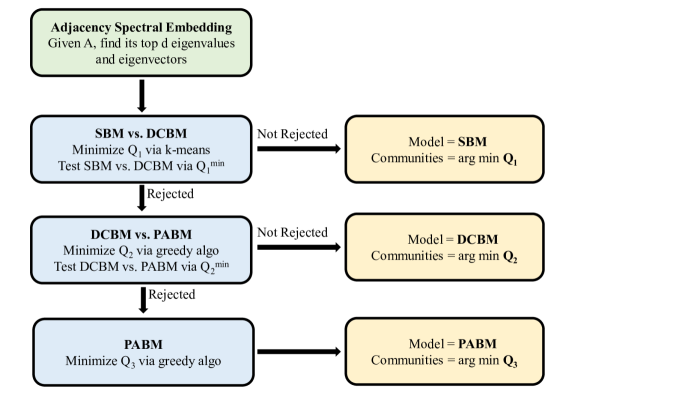
Figure 1: Visual schematic of the proposed workflow

Algorithm 1 Unified Framework for Community Detection and Model Selection

0: Adjacency matrix $A\in\{0,1\}^{n\times n}$, number of communities $K$

0: Estimated community labels $\{\widehat{\tau}_{i}\}$, selected model

1: Perform adjacency spectral embedding to compute top $d$ eigenvectors

2: Set $d=K$, compute $Q_{1}^{\min}=\min_{\{t_{i}\}}Q_{1}(\{t_{i}\};\{\widehat{U}_{i}\})$ using K-means

3: Perform parametric bootstrap to test $H_{0}:A\sim\mathrm{SBM}\quad\text{vs.}\quad H_{1}:A\sim\mathrm{DCBM}$

4: if p-value $\geq\alpha$ then

5:  return  $\{\widehat{\tau}_{i}\}=\arg\min Q_{1}(\cdot;\{\widehat{U}_{i}\})$, Model: SBM

6: end if

7: Set $d=K$, compute $Q_{2}^{\min}=\min_{\{t_{i}\}}Q_{2}(\{t_{i}\};\{\widehat{U}_{i}\})$ using greedy algorithm

8: Perform parametric bootstrap to test $H_{0}:A\sim\mathrm{DCBM}\quad\text{vs.}\quad H_{1}:A\sim\mathrm{PABM}$

9: if p-value $\geq\alpha$ then

10:  return  $\{\widehat{\tau}_{i}\}=\arg\min Q_{2}(\cdot;\{\widehat{U}_{i}\})$, Model: DCBM

11: end if

12: Set $d=K^{2}$, compute $Q_{3}^{\min}=\min_{\{t_{i}\}}Q_{3}(\{t_{i}\};\{\widehat{U}_{i}\})$ using greedy algorithm

13: return  $\{\widehat{\tau}_{i}\}=\arg\min Q_{3}(\cdot;\{\widehat{U}_{i}\})$, Model: PABM

3 Theoretical results

In this section, we establish the theoretical foundations of our unified framework for community detection and model selection under the SBM, DCBM, and PABM. Under each model, we prove exact label recovery for community detection as well as consistency of Type-1 error and power. We first state a result for the Frobenius and $2\to\infty$ norm estimation of the latent positions $U$.

Lemma 3.1.

Let $A$ be an edge-independent random graph with edge probability matrix $P\in[0,1]^{n\times n}$, where $P$ has rank $r$ and $r$ is a constant independent of $n$. Let $\widehat{U}$ and $U$ be $n\times r$ matrices whose columns are the leading eigenvectors of $A$ and $P$ respectively. Let $\delta(P):=\max\limits_{i\in[n]}\sum_{j=1}^{n}P_{ij}$ and $d_{r}(P)$ denote the maximum expected degree and smallest (in magnitude) non-zero eigenvalue of $P$, respectively. Suppose that $\delta(P)=\Omega(\log n)$ for all $n\in\mathbb{N}$ and $|d_{r}(P)|\geq c_{0}\,\delta(P)$ for some constant $c_{0}$. Denote by $\mathbb{O}_{r}$ the set of $r\times r$ orthogonal matrices. Then for any constant $c>0$, there exist constants $C>0$ and $n_{0}>0$, both possibly depending on $c$, such that for all $n\geq n_{0}$ we have

$$\min_{W\in\mathbb{O}_{r}}\|\widehat{U}W-U\|_{F}^{2}\leq\frac{C}{\delta(P)},$$ (12)

$$\min_{W\in\mathbb{O}_{r}}\|\widehat{U}W-U\|_{2\to\infty}\leq\frac{C\log^{\frac{1}{2}}{n}}{n^{\frac{1}{2}}\delta(P)^{\frac{1}{2}}},$$ (13)

with probability at least $1-n^{-c}$.

Eq. (12) follows from the Davis-Kahan theorem and standard matrix concentration bounds for $\|A-P\|$ (see e.g., Oliveira (2009); Bandeira and Van Handel (2016); Tropp (2012)), while Eq. (13) is an adaptation/simplification of Theorem 3.2 in Xie (2024) to the setting of the current paper (a similar result is also provided in Cape et al. (2019a) but with a slightly worse lower bound condition for $\delta(P)$). As $U$ (resp. $\widehat{U}$) is not unique unless the $r$ largest eigenvalues of $P$ (resp. $A$) are distinct, these Frobenius and $2\to\infty$ norm bounds involve minimization over orthogonal matrices $W$ to align the subspaces for $\widehat{U}$ and $U$. For ease of exposition, we shall omit the dependency on this alignment in the subsequent discussion as it has no impact on the theoretical results presented; more specifically, our inference procedures only depend on the Euclidean distance between the rows of $\widehat{U}$ and thus yield the same performance when applied to $\widehat{U}W$ for any arbitrary orthogonal matrix $W$.

3.1 Stochastic blockmodel

Let us consider an SBM with parameter $\Omega$ as defined in (1). By Lemma 3.1 of Lei and Rinaldo (2015), there exists a $K\times K$ matrix $H$ with orthonormal rows such that

$$U_{i}=n_{\tau_{i}}^{-\frac{1}{2}}H_{\tau_{i}}$$ (14)

for all $i\in[n]$, where $n_{k}=|\mathcal{G}_{k}|$ for all $k\in[K]$, and $U_{i}$ and $H_{k}$ are the $i^{th}$ and $k^{th}$ row of $U$ and $H$, respectively. Define $n_{\min}=\min_{k}n_{k},\,n_{\max}=\max_{k}n_{k}$. Let $\delta(P)=\max_{i}\sum_{j=1}^{n}P_{ij}$ denote the maximum expected degree. The assumptions we are going to consider are

• The communities are balanced, that is, there exists a constant $c>0$ such that

  $$\frac{n}{cK}\leq n_{k}\leq\frac{c\,n}{K},\ \text{for all }k\in[K].$$

• $d_{K}\geq c_{0}\,\delta(P)$ for some constant $c_{0}>0$, $\delta(P)=\omega(\log n)$.

A1 is the balanced communities assumption, which says that the community sizes are of the same order. A2 is a lower bound on the sparsity of the network.

We are now ready to state the theoretical results under the SBM. The following theorem shows that when the network is generated from an SBM, minimizing the objective function $Q_{1}$ using $K$-means on spectral embeddings leads to exact recovery of the true community labels with high probability. Moreover, the minimized objective function, $Q_{1}^{\min}$, remains small under the SBM with probability going to 1. We note that strong consistency under the SBM is not a new result in itself (Sussman et al., 2012; Lei and Rinaldo, 2015), but the additional result proving an upper bound on the objective function is new and critical for model selection, since it validates the use of $Q_{1}^{\min}$ as a test statistic for distinguishing the SBM from more complex models.

Theorem 3.1.

Suppose $A$ is the adjacency matrix of a network from the SBM with parameter $\Omega$ as defined in Eq. (1). Let Assumptions A1-A2 hold. Let $\{\widehat{\tau}_{i}\}$ be a global minimizer of $Q_{1}(\{t_{i}\};\{\widehat{U}_{i}\})$. Then,

$$Q_{1}(\{\widehat{\tau}_{i}\};\{\widehat{U}_{i}\})=O(\delta(P)^{-1})$$

with high probability. Furthermore, there exists a bijection $\sigma:[K]\mapsto[K]$ such that

$$\sum_{i=1}^{n}\mathbb{I}(\widehat{\tau}_{i}\not=\sigma(\tau_{i}))=0$$

with high probability, i.e., $\widehat{\tau}$ achieves exact recovery of $\tau$.

3.2 Degree-corrected blockmodel

We now consider a DCBM with parameters $\Omega$ and $\{\theta_{i}\}_{1\leq i\leq n}$, as defined in (2). Define $\theta_{\min}=\min_{i}\theta_{i},\,\theta_{\max}=\max_{i}\theta_{i}$. Let $\phi_{k}\in\mathbb{R}^{n}$ be a vector which agrees with $\theta$ on $\mathcal{G}_{k}$ and 0 elsewhere. Let $\widetilde{\phi}_{k}=\phi_{k}/\left\|\phi_{k}\right\|$ and $\widetilde{\theta}=\sum_{k=1}^{K}\widetilde{\phi}_{k}$. By Lemma 4.1 of Lei and Rinaldo (2015), there exists a $K\times K$ matrix $H$ with orthonormal rows such that

$$U_{i}\,=\,\widetilde{\theta}_{i}\,H_{\tau_{i}}$$ (15)

for all $i\in[n]$, where $H_{k}$ is the $k^{th}$ row of $H$.

The next theorem is regarding the behavior of $Q_{1}$ under the DCBM. It shows that when the network is generated from a DCBM with sufficient degree heterogeneity, the minimized objective function, $Q^{\min}_{1}$, is greater than $1/\delta(P)$ with high probability for any choice of community assignments. This result, in conjunction with the second part of Theorem 3.1, ensures the asymptotic power of the SBM vs. DCBM test and validates the rejection of the SBM in favor of the DCBM as long as there is sufficient variation among the $\theta_{i}$’s.

Theorem 3.2.

Let $A$ be the adjacency matrix of a network from the DCBM with parameters $\Omega$ and $\{\theta_{i}\}_{1\leq i\leq n}$ as defined in Eq. (2). Let Assumptions A1-A2 hold. Furthermore, suppose $\theta_{\max}/\theta_{\min}=O(1)$ and

$$\frac{1}{n_{\max}}\sum_{k=1}^{K}\sum_{i\colon\tau_{i}=k}(\theta_{i}-\bar{\theta}_{k})^{2}\gg\frac{1}{\delta(P)},\quad\text{ where }\bar{\theta}_{k}=\frac{1}{n_{k}}\sum_{i\colon\tau_{i}=k}\theta_{i}.$$ (16)

Then for any community assignment $\{t_{i}\}$, we have

$$Q_{1}(\{t_{i}\};\{\widehat{U}_{i}\})\gg 1/\delta(P)$$

with high probability.

Remark 3.1.

Theorem 3.2 states that if there is sufficient heterogeneity among the degree parameters $\{\theta_{i}\}$ generating the DCBM network in the form of Eq. (16), then the test based on $Q_{1}$ has an asymptotic power of 1. If the entries of $\Omega$ scales with a sparsity parameter $\rho_{n}$, then $\delta(P)\asymp n\rho_{n}$, and Eq. (16) reduces to

$$\frac{1}{n_{\max}}\sum_{k=1}^{K}\sum_{i\colon\tau_{i}=k}(\theta_{i}-\bar{\theta}_{k})^{2}\gg 1/(n\rho_{n}).$$ (17)

Lei (2016) imposes a similar restriction on the heterogeneity of the degree parameters for the goodness-of-fit test (see Theorem 3.5 of Lei (2016)). Under the assumptions of Theorem 3.2, Lei’s test has asympotitcally power 1 provided there exists a community $k\in[K]$ such that

$$\frac{1}{n_{\max}}\min_{u\,\in\,\mathbb{R}^{n_{\kern-0.73616ptk}}}\left\{\sum_{i:\,\tau_{i}=k}(\theta_{i}-u)^{2}:u\ \text{has at most $K$ distinct values}\right\}\gg 1/(n^{\frac{1}{2}}\rho_{n}).$$ (18)

Clearly, Eq. (17) is a much weaker condition than Eq. (18), which implies that the proposed test is asymptotically more powerful than the goodness-of-fit test by Lei (2016).

Our next result shows that minimizing $Q_{2}$ leads to exact label recovery of $\tau$ under a DCBM. We note that there are existing community detection methods in the literature that also achieve exact label recovery. This theorem shows that the proposed community detection achieves comparable accuracy. Furthermore, it also shows that $Q^{\min}_{2}$ is small under the DCBM, justifying its role as a test statistic for model selection.

Theorem 3.3.

Suppose $A$ is the adjacency matrix of a network from the DCBM with parameters $\Omega$ and $\{\theta_{i}\}_{1\leq i\leq n}$ as defined in Eq. (2). Let Assumptions A1-A2 hold and that $\theta_{\max}/\theta_{\min}=O(1)$. Let $\{\widehat{\tau}_{i}\}$ be a global minimizer of $Q_{2}(\{t_{i}\};\{\widehat{U}_{i}\})$. Then

$$Q_{2}(\{\widehat{\tau}_{i}\};\{\widehat{U}_{i}\})=O(\delta(P)^{-1})\text{ with high probability},$$

and there exists a bijection $\sigma:[K]\mapsto[K]$ such that

$$\sum_{i=1}^{n}\mathbb{I}(\widehat{\tau}_{i}\not=\sigma(\tau_{i}))=0$$

with high probability, i.e., $\widehat{\tau}$ achieves exact recovery of $\tau$.

3.3 Popularity-adjusted blockmodel

Let us consider a PABM with popularity parameters $\Lambda$ as defined in Eq. (3). Let $UDU^{\top}$ be the eigendecomposition of $P$, where

$$D=\mathrm{diag}(d_{1},\ldots,d_{K^{2}}),|d_{1}|\geq|d_{2}|\geq\ldots\geq|d_{K^{2}}|>0.$$

We now note a few simple properties of $U$ that is essential to the subsequent discussion. First assume, without loss of generality, that the rows of $U$ are ordered in increasing order of the true community assignments $\tau$, i.e., $\tau_{i}\leq\tau_{j}$ for all $i\leq j$. Next, for any $(k,\ell)\in[K]\times[K]$, let $\lambda^{(k\ell)}=(\lambda_{i\ell}\colon\tau_{i}=k)$ denote the vector in $\mathbb{R}^{n_{k}}$ whose elements are the affinities toward the $\ell^{th}$ community of all vertices in the $k^{th}$ community. Define

$$\Lambda^{(k)}=[\lambda^{(k1)}\mid\lambda^{(k2)}\mid\dots\mid\lambda^{(kK)}]\in\mathbb{R}^{n_{k}\times K},\quad X=\begin{bmatrix}\Lambda^{(1)}&0&0&\dots&0\\ 0&\Lambda^{(2)}&0&\dots&0\\ \vdots&\vdots&\ddots&\vdots&\vdots\\ 0&0&\dots&0&\Lambda^{(K)}\end{bmatrix}\in\mathbb{R}^{n\times K^{2}}.$$

Then from the proof of Theorem 2 in Koo et al. (2022), we have $UU^{\top}=X(X^{\top}X)^{-1}X^{\top}$, and hence, $U=X(X^{\top}X)^{-\frac{1}{2}}W$ for some orthogonal matrix $W$. Let $Z=X(X^{\top}X)^{-\frac{1}{2}}$. Then $Z$ have the same block diagonal structure as $X$, i.e,

$$Z=\begin{bmatrix}Z^{(1)}&0&0&\dots&0\\ 0&Z^{(2)}&0&\dots&0\\ \vdots&\vdots&\ddots&\vdots&\vdots\\ 0&0&\dots&0&Z^{(K)}\end{bmatrix},Z^{\top}Z=\begin{bmatrix}Z^{(1)\top}Z^{(1)}&0&0&\dots&0\\ 0&Z^{(2)\top}Z^{(2)}&0&\dots&0\\ \vdots&\vdots&\ddots&\vdots&\vdots\\ 0&0&0&\dots&Z^{(K)\top}Z^{(K)}\end{bmatrix}=I_{K^{2}},$$

where $Z^{(k)}$ is a $n_{k}\times K$ matrix for all $k\in[K]$. If a matrix $\mathcal{P}$ is symmetric idempotent, then $W\mathcal{P}W^{\top}$ is symmetric idempotent for any orthogonal $W$ and $\|(I-\mathcal{P})U_{i}\|=\|(I-W\mathcal{P}W^{\top})(WU_{i})\|$ for all $i$. Therefore, we can assume without loss of generality that $U=Z$ so that $\sum_{i\colon\tau_{i}=k}\|U_{i}\|^{2}=\|Z^{(k)}\|_{F}^{2}=\mathrm{tr}[Z^{(k)\top}Z^{(k)}]=K$.

We make the following assumptions for the node popularity vectors $\lambda_{i}=(\lambda_{i1},\dots,\lambda_{iK})$:

• The communities are balanced, that is, there exists $c>0$ such that

  $$\frac{n}{c\,K}\leq n_{k}\leq\frac{c\,n}{K},\ \text{for all }1\leq k\leq K.$$

• $|d_{K^{2}}|\geq c_{0}\,\delta(P)$ for some constant $c_{0}>0$, $\delta(P)=\omega(\log n)$.

• There exists a sequence $\{\rho_{n}\}$ such that $\|\Lambda\|_{2\rightarrow\infty}=\rho_{n}^{\frac{1}{2}}$, and there exists a constant $\gamma_{1}>0$ such that $\|\lambda_{i}\|\geq\gamma_{1}\,\rho_{n}^{\frac{1}{2}}$ for all $i\in[n]$.

• There exists a constant $\gamma_{2}>0$ such that for any $k\in[K]$, and any subset of nodes $\mathcal{S}$ from community $k$ with $|\mathcal{S}|\geq n_{k}/K$, we have

  $$\sigma_{\min}\left(\sum_{i\,\in\,\mathcal{S}}\lambda_{i}\lambda_{i}^{\top}\right)\,\geq\,\gamma_{2}\,\frac{n_{k}\rho_{n}}{K},$$

  where $\sigma_{\min}(\cdot)$ denote the smallest singular value of a matrix.

B1 is the balanced communities assumption, which says that the community sizes are of the same order. B2 is a lower bound on the sparsity of the network. B3 is a standard homogeneity condition on the scale of the latent position vectors. The quantity $\rho_{n}$ introduced in B3 can be interpreted as a sparsity parameter, and B2 implies that $n\rho_{n}$ must be $\omega(\log n)$. B4 states that any sufficiently large collection of vertices from a given community $k$ will have latent positions that cover (in volume) a non-negligible region of $\Lambda^{(k)}$.

Our next result derives the behavior of the objective function $Q_{2}$ under the PABM. Recall that, when the true model is DCBM, the latent positions lie in distinct 1-dimensional subspaces, one for each community. However, under the PABM, the true latent positions reside in a higher-dimensional space, specifically in the span of the top $K^{2}$ eigenvectors of the population matrix $P$. To study the behavior of $Q_{2}$ under the PABM, we must therefore analyze the properties of the $K$-dimensional vector embeddings derived from the top $K$ eigenvectors of $P$, which no longer coincide with the true latent positions. This is different from the SBM vs. DCBM case, where the latent positions are nested. Assuming $|d_{K}|>|d_{K+1}|$, let $\widetilde{U}$ denote the matrix of the first $K$ eigenvectors of $P$, and $\widehat{\widetilde{U}}$ be its empirical counterpart. The following theorem shows that, under the PABM, if the rows of $\widetilde{U}$ span higher-dimensional subspaces across communities, then $Q_{2}$ exceeds $1/\delta(P)$ for any community assignment. This guarantees that the DCBM vs. PABM test achieves power tending to one under the PABM alternative.

Theorem 3.4.

Suppose $A$ is the adjacency matrix of a network from the PABM with parameter $\Lambda$ as defined in 3. Let Assumptions B1-B2 hold. Suppose that there exists at least one community $k\in[K]$ such that for any subset of nodes $\mathcal{S}$ of size at least $n_{k}/K$ from that community,

$$\sigma_{2}(\widetilde{U}_{\mathcal{S}})\gg 1/\delta(P),$$ (19)

where $\widetilde{U}_{\mathcal{S}}\in\mathbb{R}^{K\times|\mathcal{S}|}$ is the matrix consisting of columns $\widetilde{U}_{i},\,i\in\mathcal{S}$, and $\sigma_{2}(.)$ denotes the second largest singular value of a matrix.

Then for any community assignment $\{t_{i}\}$, we have

$$Q_{2}(\{t_{i}\};\{\widehat{\widetilde{U}_{i}}\})\,\gg\,1/\delta(P).$$

with high probablity.

The condition (19) states that for any sufficiently large collection of vertices from a given community $k$, the $K$-dimensional embeddings $\{\widetilde{U}_{i}\}$ cannot be well approximated by a 1-dimensional subspace in $\mathbb{R}^{K}$.

Our final theorem shows that the proposed objective function $Q_{3}$, which clusters spectral embeddings using rank-$K$ projections, yields exact community recovery under the PABM. It validates the final step of the model selection workflow in Figure 1, ensuring that both clustering and model selection are consistent under the PABM.

Theorem 3.5.

Suppose $A$ is the adjacency matrix of a network from the PABM with parameters $\Lambda$ as defined in Eq. (3). Let Assumptions B1-B4 hold and $\{\widehat{\tau}_{i}\}$ be a global minimizer of $Q_{3}(\{t_{i}\};\{\widehat{U}_{i}\})$. Then

$$Q_{3}(\{\widehat{\tau}_{i}\};\{\widehat{U}_{i}\})=O(\delta(P)^{-1})\ \text{with high probability.}$$ (20)

Furthermore, there exists a bijection $\sigma:[K]\mapsto[K]$ such that

$$\sum_{i=1}^{n}\mathbb{I}(\widehat{\tau}_{i}\neq\sigma(\tau_{i}))=0$$

with high probability.

Remark 3.2.

In this paper, we proposed and empirically evaluated a parametric bootstrap strategy for model selection, although we did not provide a formal proof of its validity. In recent years, there has been significant progress in the theoretical understanding of bootstrapping techniques for network data, with notable contributions from Bhattacharyya and Bickel (2015); Green and Shalizi (2022); Lunde and Sarkar (2022); Levin and Levina (2025). However, none of these existing results apply to the objective functions $Q_{1}$, $Q_{2}$, and $Q_{3}$ proposed in this paper. As a result, new theoretical tools are required to establish bootstrap consistency for our proposed methodology. Developing such a foundation remains an important direction for future research.

4 Simulation study

In this section, we assess the empirical performance of our proposed framework for community detection and model selection under the three blockmodels, as well as the nested blockmodel proposed by Noroozi and Pensky (2021). Wherever existing methods are available, we compare the proposed approach against state-of-the-art methods. Note that there are no existing methods for testing the DCBM vs. the PABM. The results demonstrate that our methodology achieves high accuracy both for label recovery and model selection consistency throughout. In particular, the proposed workflow either outperforms or matches existing approaches across a range of network settings.

4.1 Community detection

We first analyze the performance of our proposed community detection methods for the three blockmodels under consideration. We refer to the community detection methods for SBM, DCBM, and PABM as $Q_{1}$, $Q_{2}$, and $Q_{3}$, respectively. The assessment metric of interest is the mislabeling rate, and the results are presented in Tables 1, 2 and 3, respectively.

4.1.1 Stochastic blockmodel

We generated networks from the SBM with $n$ nodes and $K=3$ communities with 25%, 25% and 50% nodes in the 3 communities, respectively. The block probability matrix,

$$\Omega\propto\begin{pmatrix}4&2&1\\ 2&4&1\\ 1&1&4\end{pmatrix},$$

$n$ is varied over $(1000,2000,3000)$ and the network density, $\delta$, is set to $0.05$. We simulated 100 networks for each combination of $(n,K)$. We compared the performance of $Q_{1}$ with spectral clustering using the Laplacian matrix (SC-L) (Rohe et al., 2011; Sengupta and Chen, 2015), where the $K$-means algorithm is applied on the spectral embeddings of the Laplacian matrix $L=D^{-\frac{1}{2}}AD^{-\frac{1}{2}}$ instead of the adjacency matrix.

$n$	$K$	$\delta$	$Q_{1}$	SC-L
1000	3	0.05	0.02 $\pm$ 0.007	0.02 $\pm$ 0.006
2000	3	0.05	0.00 $\pm$ 0.001	0.00 $\pm$ 0.001
3000	3	0.05	0.00 $\pm$ 0.000	0.00 $\pm$ 0.000

Table 1: Average mislabeling error $\pm$ s.e. under SBM for $Q_{1}$ and SC-L

The average mislabeling errors (proportion of mislabeled nodes) from applying $Q_{1}$ and SC-L on the networks are reported in Table 1. We observe that as $n$ increases, $Q_{1}$ recovers the true communities perfectly, that is, the proportion of mislabeled nodes goes to zero. We also find that for all choices of $(n,K)$, there is no significant difference between $Q_{1}$ and SC-L in terms of mislabeling errors.

4.1.2 Degree-corrected blockmodel

We generated networks from the DCBM with a similar configuration as before. The community sizes and the block probability matrix remains the same, and the degree parameters $\{\theta_{i}\}$ are sampled independently from the $\mathrm{Beta}(1,5)$ distribution to emulate power-law type behavior in node degrees. The number of nodes, $n$, is varied over $(1000,2000,3000)$ and the network density, $\delta$, is set to $0.05$. For comparison, we considered regularized spectral clustering using the Laplacian matrix (RSC-L), where the spectral embeddings of the Laplacian matrix are normalized before applying the $K$-means algorithm. The additional normalization step removes the effect of the multiplicative factor in the spectral embeddings for DCBM.

$n$	$K$	$\delta$	$Q_{2}$	RSC-L
1000	3	0.05	0.08 $\pm$ 0.011	0.09 $\pm$ 0.011
2000	3	0.05	0.04 $\pm$ 0.004	0.05 $\pm$ 0.005
3000	3	0.05	0.03 $\pm$ 0.003	0.03 $\pm$ 0.004

Table 2: Average mislabeling error $\pm$ s.e. under DCBM for $Q_{2}$ and RSC-L

The results are presented in Table 2. We observe that as $n$ increases, the proportion of mislabeled nodes for both $Q_{2}$ and RSC-L decreases. Moreover, there is no significant difference between $Q_{2}$ and RSC-L in terms of the mislabeling errors.

4.1.3 Popularity-adjusted blockmodel

We generated networks from the PABM with $n$ nodes and $K$ equal-sized communities, varying $n$ over $(600,900,1500)$ and $K$ over $(2,3)$. For $K=2$, the node popularity matrix $\Lambda$ is chosen such that

$$\Lambda=\begin{pmatrix}\mathbf{v}_{11}&\mathbf{v}_{12}\\ \mathbf{v}_{21}&\mathbf{v}_{22}\end{pmatrix},$$

and similarly for $K=3$, we consider

$$\Lambda=\begin{pmatrix}\mathbf{v}_{11}&\mathbf{v}_{12}&\mathbf{v}_{13}\\ \mathbf{v}_{21}&\mathbf{v}_{22}&\mathbf{v}_{23}\\ \mathbf{v}_{31}&\mathbf{v}_{32}&\mathbf{v}_{33}\end{pmatrix},$$

where the vectors $\mathbf{v}_{k\ell}\in\mathbb{R}^{n_{k}},\ 1\leq k,\,\ell\leq K$. The elements of $\mathbf{v}_{kk}$ are generated independently from the $\mathrm{Beta}(2,1)$ distribution and for $k\neq l$, the elements of $\mathbf{v}_{k\ell}$ are generated independently from the $\mathrm{Beta}(1,2)$ distribution, imposing a homophilic community structure. We applied $Q_{3}$ to 100 networks simulated for each combination of $(n,K)$, and for comparison, we analyzed the Orthogonal Subspace Clustering algorithm (OSC) proposed in Koo et al. (2022).

$n$	$K$	$\delta$	$Q_{3}$	OSC
600	2	0.28	0.02 $\pm$ 0.007	0.02 $\pm$ 0.055
900	2	0.28	0.01 $\pm$ 0.004	0.01 $\pm$ 0.051
1500	2	0.28	0.00 $\pm$ 0.001	0.00 $\pm$ 0.001
600	3	0.33	0.12 $\pm$ 0.044	0.10 $\pm$ 0.109
900	3	0.33	0.03 $\pm$ 0.018	0.03 $\pm$ 0.080
1500	3	0.33	0.00 $\pm$ 0.002	0.00 $\pm$ 0.031

Table 3: Average mislabeling error $\pm$ s.e. under PABM for $Q_{3}$

In Table 3, we see that under both settings, the average mislabeling error for both $Q_{3}$ and OSC goes to zero as $n$ increases. We also observe that although the average error rates for the two methods are similar, the standard errors for OSC are slightly ‘higher’ than $Q_{3}$ for most of the cases (except $n=1500,K=2$). To understand this pattern, we looked into the individual error rates for both methods. We found that for a few of the replications, OSC returned very poor community estimates, thus resulting in a high error, while for the rest of the replications, it performed very well, often better than $Q_{3}$. On the other hand, the performance of $Q_{3}$ is more consistent and is less affected by such bad samples. From a methodological perspective, the two algorithms use the same matrix $\widehat{U}$ of the leading eigenvector of $A$ for clustering. $Q_{3}$ attempts to cluster the rows of $\widehat{U}$ into subspaces via a $K$-means type algorithm, except that we have distinct projection matrices instead of distinct mean vectors corresponding to the clusters. Whereas, OSC attempts to cluster the rows of $\widehat{U}\widehat{U}^{\top}$ via spectral clustering (spectral decomposition + standard $K$-means). Thus, apart from the accuracy discussion, $Q_{3}$ is also computationally less expensive than OSC since, along with the spectral decomposition of $A$, OSC involves the extra step of performing spectral decomposition of the matrix $\widehat{U}\widehat{U}^{\top}$.

Our unified framework provides three objective functions for each of the three blockmodels under consideration, allowing for a natural way to do both community detection and model selection for them. As we have found in this subsection, the derived community detection methods are at par with some of the existing community detection methods we have for SBM, DCBM, and PABM. In the next subsection, we address the problem of model selection for blockmodels, where we believe the main contribution of our paper lies.

4.2 Model selection

In this subsection, we study the performance of our proposed two-step testing procedure for model selection. We refer to the tests corresponding to the testing problems in (10) (SBM vs. DCBM) and (11) (DCBM vs. PABM) as $Q_{1}$ and $Q_{2}$ respectively. The assessment metrics of interest are the Type-1 error rate and the power of the tests.

4.2.1 SBM vs. DCBM

We generated networks from the SBM and the DCBM with $n=600$ nodes and $K$ equal-sized communities. The block probability matrix,

$$\Omega\propto(1-\beta)\,I+\beta\,\mathbf{1}\mathbf{1}^{\top}.$$

$\beta$ is the ratio of the between-block probability and the within-block probability of an edge. The smaller the value of $\beta$ is, the easier it should be to detect the communities. For the DCBM, the degree parameters $\{\theta_{i}\}$ are simulated from the power-law distribution with lower bound 1 and scaling parameter 5. We vary the number of communities $K$ over $(3,5)$, $\beta$ over $(0.2,0.5)$, and the average degree of the network over $(15,20,40)$. For each combination of $(n,\,K,\,\beta,\,\text{avg. degree})$, we simulated 100 networks and applied $Q_{1}$. 200 bootstrap samples are used to estimate the $p$-value of the test, and $H_{0}$ is rejected when the $p$-value falls below 0.05.

True model: SBM
$n$	$K$	$\beta$	avg. degree	$Q_{1}$	EigMax	EigMax-boot	ECV-$L_{2}$	ECV-dev
600	3	0.2	15	0.04	1.00	0.00	0.00	0.00
600	3	0.2	20	0.05	0.98	0.00	0.00	0.00
600	3	0.2	40	0.06	0.51	0.04	0.00	0.00
600	3	0.5	15	0.00	0.77	0.00	0.00	0.00
600	3	0.5	20	0.04	0.50	0.00	0.00	0.00
600	3	0.5	40	0.00	0.18	0.00	0.00	0.00
600	5	0.2	15	0.00	0.99	0.00	0.00	0.00
600	5	0.2	20	0.01	0.95	0.00	0.00	0.00
600	5	0.2	40	0.06	0.47	0.06	0.00	0.00
600	5	0.5	15	0.01	0.20	0.00	0.00	0.00
600	5	0.5	20	0.02	0.09	0.00	0.00	0.00
600	5	0.5	40	0.01	0.00	0.00	0.00	0.00

Table 4: Proportion of times $H_{0}:A\sim\text{SBM}$ is rejected by $Q_{1}$ and EigMax, and DCBM is selected by ECV, when the true model is SBM.

True model: DCBM
$n$	$K$	$\beta$	avg. degree	$Q_{1}$	EigMax	EigMax-boot	ECV-$L_{2}$	ECV-dev
600	3	0.2	15	1.00	1.00	0.65	0.96	0.74
600	3	0.2	20	1.00	1.00	0.95	0.99	0.99
600	3	0.2	40	1.00	1.00	1.00	1.00	1.00
600	3	0.5	15	0.73	1.00	0.27	0.53	0.36
600	3	0.5	20	0.93	1.00	0.58	0.79	0.83
600	3	0.5	40	0.93	1.00	0.87	1.00	1.00
600	5	0.2	15	0.98	1.00	0.09	0.99	0.87
600	5	0.2	20	1.00	1.00	0.75	0.99	0.95
600	5	0.2	40	1.00	1.00	1.00	1.00	1.00
600	5	0.5	15	0.95	1.00	0.00	0.43	0.32
600	5	0.5	20	0.96	1.00	0.06	0.81	0.74
600	5	0.5	40	0.99	1.00	0.48	1.00	1.00

Table 5: Proportion of times $H_{0}:A\sim\text{SBM}$ is rejected by $Q_{1}$ and and EigMax, and DCBM is selected by ECV, when the true model is DCBM.

We compared the performance of our method with two existing methods: (i) A goodness-of-fit test for SBMs proposed by Lei (2016) and (ii) The edge cross-validation(ECV) method for model selection proposed by Li et al. (2020). Lei (2016) proposed a test statistic based on the largest singular value of the residual adjacency matrix $\widetilde{A}_{ij}=(A_{ij}-\widehat{P}_{ij})/\sqrt{\widehat{P}_{ij}(1-\widehat{P}_{ij})}$, which has an asymptotic Tracy-Widom distribution when the true model is SBM. Noting that the convergence might be slow, Lei (2016) also proposed an alternative test statistic using bootstrap correction. We consider both of the proposed test statistics for comparison, and call the tests EigMax and EigMax-boot respectively. The ECV is a classification method which, given a set of candidate models (two, in our case), estimates a suitably chosen loss function using the adjacency matrix $A$ and selects the one with the minimum loss function value. Li et al. (2020) analyzed two loss functions, a least-squared loss and a binomial deviance loss, and we call the corresponding methods ECV-$L_{2}$ and ECV-dev respectively. We fully acknowledge that the comparison our method to ECV is not an apples-to-apples comparison because our method is based on a testing framework, while the ECV is based on classification using a loss function minimization criterion. Tables 4 and 5 compares the performance of the five model selection procedures when the data is generated from the SBM and the DCBM respectively. For the testing procedures, $Q_{1}$, EigMax and EigMax-boot, we report the proportion of times $H_{0}:A\sim SBM$ is rejected. For ECV-$L_{2}$ and ECV-dev, we report the proportion of times DCBM is selected as the true model.

In Table 4, we observe that when the true model is SBM, the size-estimates of $Q_{1}$ are generally below the significance level of $0.05$. We find a similar result for EigMax-boot, where the size-estimates mostly remain below the significance level of $0.05$. However, EigMax performs very poorly, as we see that the size-estimates exceed the significance level in all cases. Following Lei (2016), we attribute the poor performance of EigMax to the slow convergence of the test statistic under the null. Finally, the ECV always chose the correct model. This difference is purely because we calibrate the test for $\alpha=0.05$. The proposed test matches the target significance level, and if one wants a lower Type-1 error, this could be easily achieved by lowering the value of $\alpha$ and recalibrating the test. Note that ECV, by design, does not offer this flexibility.

When the true model is DCBM and $\beta$ is 0.2, that is, there is high homophily, $Q_{1}$ has power equal to 1 in all cases. Even when $\beta$ is 0.5 (low homophily), although the problem becomes more challenging, the powers still remain above 0.8. Moreover, $Q_{1}$ consistently has a higher power than EigMax-boot in all cases. EigMax, on the other hand, has power equal to 1 across all cases, but its reliability is questionable. As we found in Table 4, EigMax may have size much larger than the significance level, that is, it may disproportionally reject $H_{0}:A\sim SBM$ even when the true model is SBM, with identical choices of parameters. Finally, in comparison with ECV, we observe that the proportion of rejections in favor of $H_{1}:A\sim\text{DCBM}$ using $Q_{1}$ is almost consistently larger than the proportion of times DCBM is selected as the true model by ECV. However, as we said earlier, we should be cautious while interpreting the results from these two frameworks.

4.2.2 DCBM vs. PABM

We generated networks from the DCBM following the same configuration as before. Here, we kept $\beta$ fixed at 0.5, noting that it is the more difficult case to deal with. For PABM, we used the setting introduced in Section 4.1 for community detection. Here, we fixed $n=900$ and scaled $P$ so that the network density $\delta$ varies over $(0.01,0.02,0.05,0.1)$. For each scenario, we simulated 100 networks and applied $Q_{2}$. As before, we used 200 bootstrap samples to estimate the $p$-value of the test and rejected $H_{0}$ when it fell below 0.05. The results for DCBM and PABM are presented in Tables 6 and 7 respectively.

$n$	$K$	$\beta$	avg. degree	$Q_{2}$
600	3	0.5	15	0.00
600	3	0.5	20	0.01
600	3	0.5	40	0.03
600	5	0.5	15	0.03
600	5	0.5	20	0.01
600	5	0.5	40	0.02

Table 6: Proportion of times $H_{0}:A\sim\text{DCBM}$ is rejected by $Q_{2}$ when the true model is DCBM

$n$	$K$	$\delta$	$Q_{2}$
900	2	0.01	0.44
900	2	0.02	1.00
900	2	0.05	1.00
900	2	0.10	1.00
900	3	0.01	0.00
900	3	0.02	0.14
900	3	0.05	1.00
900	3	0.10	1.00

Table 7: Proportion of times $H_{0}:A\sim\text{DCBM}$ is rejected by $Q_{2}$ when the true model is PABM

We observe that when the true model is DCBM (Table 6), the size of the test is always less than the significance level of $0.05$. When the true model is PABM (Table 7), the power of the test is 1 when except when the network density is small, that is, the network is too sparse. We know that if a network is too sparse, the latent position estimation as well as the community estimation problem becomes harder, which possibly leads to a small power in this case.

4.2.3 Nested stochastic blockmodel

Next, we applied $Q_{2}$ on networks generated from the nested stochastic blockmodel (NBM), proposed by Noroozi and Pensky (2021). Observing the significant jump in the parameters from DCBM to PABM, the NBM was proposed as a bridge between the DCBM and PABM in the hierarchy of blockmodels. The NBM has $K$ communities and $L$ meta-communities, where each meta-community is composed of members from exactly one or more of the $K$ communities, that is, $L\leq K$. When $L=1$, the NBM reduces to the DCBM, and for $L=K$, the NBM becomes a PABM. To generate networks from the NBM, we used the same simulation setting as the one considered in Section 7.1 of Noroozi et al. (2021). We refer the readers to Noroozi and Pensky (2021) for details on generating the model parameters. Along with $n,K,$ and $L$, there is an additional factor $\omega$ which captures the homophily in the network, such that as $\omega$ increases, the community estimation and, subsequently, the model selection task become harder.

$n$	$K$	$L$	$\omega$		$Q_{2}$
900	6	1	0.6		0.00
900	6	1	0.8		0.24
900	6	2	0.6		0.86
900	6	2	0.8		0.93
900	6	3	0.6		1.00
900	6	3	0.8		1.00
900	6	6	0.6		1.00
900	6	6	0.8		1.00

$n$	$K$	$L$	$\omega$		$Q_{2}$
1260	6	1	0.6		0.00
1260	6	1	0.8		0.09
1260	6	2	0.6		0.75
1260	6	2	0.8		0.93
1260	6	3	0.6		1.00
1260	6	3	0.8		1.00
1260	6	6	0.6		1.00
1260	6	6	0.8		1.00

Table 8: Proportion of times $H_{0}:\text{DCBM}$ is rejected by $Q_{2}$ when the true model is NBM ($L=1$ corresponds to DCBM, and $L=K$ corresponds to PABM)

In Table 8, we observe that when $L=1$, that is, the true model is DCBM, the size of the test is 0 for $\omega=0.6$, that is, when there is high homophily. For $\omega=0.8$ (low homophily), the power is 0.24 and 0.09 when $n$ is $900$ and $1260$, respectively, which is larger than the desired significance level of 0.05. Next, we observe that as $L$ increases, the model becomes more and more complex than the DCBM, and it gradually becomes easier for the test to correctly reject $H_{0}$. When $L=2$, the power of the test is high (above 0.75 for all values of $n$, $K$, and $\omega$), although still below 1. When $L=3$ and $6$, the power of the test is 1, that is, the test is always rejected.

5 Application to real-world datasets

We applied our model selection procedure to five real-world networks that have been well-studied in the statistical network literature and are known to have a community structure: the Karate Club network, the Dolphin network, the British MP’s Twitter network, the political blogs network, and the DBLP network. For each network, our goal is to determine which of the three blockmodels would best fit the network. We first briefly describe the five networks and then discuss the results of our analysis.

Karate club: The Karate club network is a network of social ties between 34 members of a university Karate club, studied by Wayne W. Zachary over a three-year period from 1970 to 1972 (Zachary, 1977). During his study, a conflict arose between the administrator and the instructor of the club, eventually leading to the club’s split into two new clubs, centered around the administrator and the instructor. The communities of club members were determined by which new club they decided to join. This network was shown as a classic example of community structure by Girvan and Newman (2002).

Dolphin: The Dolphin network is a network of social links between 62 bottlenose dolphins living in Doubtful Sound, Fiordland, New Zealand, studied by Lusseau (2003) from November 1994 to November 2001. The authors photo-identified 1292 schools of dolphins during the seven-year period, and two dolphins were linked if they were seen together in a school more often than average. The original paper found two large groups and a very small group using cluster analysis on the network. For our analysis, we assumed $K=2$ communities in the network.

British MP: The British MPs Twitter dataset consists of 419 Members of Parliament (MP) in the United Kingdom belonging to five different political parties, and there are three layers of networks between them representing three types of connections, namely, follows, mentions and retweets on the social media platform Twitter (Greene and Cunningham, 2013). For our analysis, we considered the network of retweets. We picked a subset of this network consisting of 360 MPs belonging to the Conservative Party and the Labour Party, the two parties with the highest number of members in the dataset. We analyzed the largest connected component of this subnetwork, which had 329 nodes and 5720 edges.

Political blogs: The political blogs network is a network of hyperlinks between 1454 political blogs in the United States of America, studied over two months before the 2004 Presidential election (Adamic and Glance (2005)). Of the 1454 blogs, 759 were identified as liberal and 735 as conservative ($K=2$ communities). This network is also very popular in network science to demonstrate community structure in networks (Karrer and Newman (2011); Amini et al. (2013); Jin (2015)). For our analysis, we extracted the largest connected component of this network, consisting of 1222 nodes and 16714 edges.

DBLP: The DBLP four-area network was curated by Gao et al. (2009) and Ji et al. (2010) from the Digital Bibliography & Library Project (DBLP), a computer science bibliographical database. The original dataset consists of 14376 papers written by 14475 authors from four research areas related to data mining: database, data mining, information retrieval, and artificial intelligence ($K=4$). We analyzed a network formed by 4057 of the 14475 authors for which the true research areas were known, and two authors were assigned an edge if they published their work at the same conference. This network was also studied in Sengupta and Chen (2015) in the context of spectral clustering in heterogeneous networks.

Network	Attributes		$H_{0}:$ SBM vs. $H_{1}:$ DCBM		$H_{0}:$ DCBM vs. $H_{1}:$ PABM
	$n$	$K$	$H_{0}$ rejected?	$p$-value	$H_{0}$ rejected?	$p$-value
Karate club	34	2	✓	0.03	✗	0.29
Dolphin	62	2	✓	0.01	✗	0.75
British MP	329	2	✓	0.00	✓	0.00
Political blogs	1222	2	✓	0.00	✓	0.00
DBLP	4057	4	✓	0.00	✓	0.00

Table 9: Results from performing the two tests for blockmodels on five real-world networks

In Table 9, we report the outputs of the model selection procedure on these five networks. We first test if the given network can be modeled by the SBM, against, if it should be modeled as a DCBM.  We find that for all the five networks, the test is rejected. We know that the SBM is the simplest network model to incorporate community structure. While many real-world networks exhibit community structure, we are not surprised if they can not be well-represented by the SBM. Next, we test if the given network can be modeled by the DCBM, against, if we would need a more complicated blockmodel, such as PABM, to model it. We find that for two of our networks, the Karate Club network and the Dolphin network, the test is not rejected. Therefore, the conclusion is that while the SBM is not good enough to model these two networks, the DCBM is able to explain the community structure very well. The other three networks, the British MPs network, the political blogs network, and the DBLP network, are still rejected, concluding that they can not be accurately represented by the DCBM as well.

6 Discussion

In this paper, we presented a unified framework to perform community detection and model selection by utilizing the nested structure of the blockmodels: SBM, DCBM, and PABM. Through a detailed simulation study, we showed that given a network generated from one of these models, the proposed method is able to select the correct model as well as estimate the true community assignments accurately. We derived the theoretical properties of the proposed objective functions under SBM and DCBM, and discussed the theoretical challenges for PABM related to subspace clustering. One important direction of our future research will be to develop a formal proof of the parametric bootstrap strategy we used to estimate the $p$-value of our tests for model selection.

This paper does not include some notable variants of blockmodels, such as the mixed-membership stochastic blockmodel (MMSBM Airoldi et al. (2009)) and the degree-corrected mixed-membership model (DCMM, Jin et al. (2023)). This is because the unified spectral framework that forms the basis of the proposed workflow does not cover these models. Another important direction of future research would be to extend the proposed framework to these models.

Supplementary material for “ A Unified Framework for Community Detection and Model Selection in Blockmodels”

A1 Proof of Theorem 3.1

Proof.

For $k\in[K]$, define

$$\mathcal{C}^{(\tau,\widehat{U})}_{k}=\frac{1}{n_{k}}\sum_{i\colon\tau_{i}=k}\widehat{U}_{i},$$

where $n_{k}=|\{i\colon\tau_{i}=k\}|$, i.e., $\{\mathcal{C}^{(\tau,\widehat{U})}_{k}\}$ are the cluster centroids for the $\{\widehat{U}_{i}\}$ as given by $\{\tau_{i}\}$. Next recall Eq. (14). Then by Lemma 3.1, we have

$$\begin{split}Q_{1}(\{\widehat{\tau}_{i}\};\{\widehat{U}_{i}\})&\leq Q_{1}(\{\tau_{i}\};\{\widehat{U}_{i}\})=\sum_{k=1}^{K}\sum_{i\colon\tau_{i}=k}\|\widehat{U}_{i}-\mathcal{C}^{(\tau,\widehat{U})}_{k}\|^{2}\\ &\leq\sum_{k=1}^{K}\sum_{i\colon\tau_{i}=k}\|\widehat{U}_{i}-U_{i}\|^{2}=\|\widehat{U}-U\|_{F}^{2}=O(\delta(P)^{-1})\end{split}$$ (A1)

with high probability, under Assumtions A1 and A2.

The exact recovery of $\widehat{\tau}$ can be shown using the same argument as that for the proof of Theorem 6 in Lyzinski et al. (2014). More specifically, let

$$r_{*}=\frac{1}{4}\min_{\tau_{i}\not=\tau_{j}}\|U_{i}-U_{j}\|=\frac{1}{4}\min_{\tau_{i}\not=\tau_{j}}\bigl{(}\|U_{i}\|^{2}+\|U_{j}\|^{2}\bigr{)}^{\frac{1}{2}}\geq(8\,n_{\max})^{-\frac{1}{2}}.$$

Note that in the above derivations we have used the fact that $K$ has orthonormal columns so that $H_{k}^{\top}H_{\ell}=0$ whenever $k\not=\ell$ together with the form for $U$ in Eq. (14). Next let $\mathcal{B}_{1},\dots,\mathcal{B}_{K}$ be $K$ balls of radii $r_{*}$ centered around the distinct rows of $U$; these balls are disjoint due to the choice of $r_{*}$. Define

$$\mathcal{C}^{(\widehat{\tau},\widehat{U})}_{k}=\frac{1}{\widehat{n}_{k}}\sum_{i\colon\widehat{\tau}_{i}=k}\widehat{U}_{i},\quad\text{for $1\leq k\leq K$},\\$$

where $\widehat{n}_{k}=|\{i\colon\widehat{\tau}_{i}=k\}|$ and let $\widehat{C}$ be the $n\times K$ matrix with rows $\widehat{C}_{i}=\mathcal{C}^{(\widehat{\tau},\widehat{U})}_{\widehat{\tau}_{i}}$.

Now condition on the high-probability event in Eq. (A1). Next, suppose there exists a $k\in[K]$ such that $\mathcal{B}_{k}$ does not contain any row of $\widehat{C}$. Then $\|\widehat{C}-U\|_{F}\geq r_{*}\sqrt{n_{\min}}$ where $n_{\min}=\min\limits_{k\in[K]}n_{k}$ is the size of the smallest community. We thus have

$$(Q_{1}(\{\widehat{\tau}_{i}\};\{\widehat{U}_{i}\}))^{\frac{1}{2}}= \|\widehat{C}-\widehat{U}\|_{F}\geq\|\widehat{C}-U\|_{F}-\|\widehat{U}-U\|_{F}$$

$$\geq r_{*}\sqrt{n_{\min}}-O(\delta(P)^{-\frac{1}{2}})=\omega((\delta(P))^{-\frac{1}{2}}),$$

a contradiction, where the final inequality is due to the fact that $n_{\min}\asymp n_{\max}$ and so $r_{*}\sqrt{n_{\min}}\asymp 1$. Therefore, by the pigeonhole principle, each ball $\mathcal{B}_{k}$ contains precisely one unique row of $\widehat{C}$.

Choose an arbitrary pair $i\not=j$. Recall that, for the $K$-means clustering criterion, each point $x$ is assign to the closest cluster centroid. Now if $\widehat{C}_{i}=\widehat{C}_{j}$, then $\widehat{U}_{i}$ and $\widehat{U}_{j}$ are assigned to the same cluster and hence they both belong to $\mathcal{B}_{k}$ for some $k$, i.e., $\|\widehat{U}_{i}-\widehat{U}_{j}\|\leq 2\,r_{*}$. Lemma 3.1 then implies

$$\|U_{i}-U_{j}\|\leq 2\,\|\widehat{U}-U\|_{2\to\infty}+2\,r_{*}=O\left(\frac{\log^{\frac{1}{2}}{n}}{n^{\frac{1}{2}}\delta(P)^{\frac{1}{2}}}\right)+2\,r_{*}\leq 3\,r_{*}$$

with high probability and hence $U_{i}=U_{j}$ as the smallest gap between any two distinct rows of $U$ is at least $4\,r_{*}$. Conversely, suppose $U_{i}=U_{j}$. Then, as $\|\widehat{U}-U\|_{2\to\infty}\leq r_{*}$ with high probability, both $\widehat{U}_{i}$ and $\widehat{U}_{j}$ belongs to the same $\mathcal{B}_{\tau_{i}}$, and since $\mathcal{B}_{\tau_{i}}$ contains a unique row of $\widehat{C}$, both $\widehat{U}_{i}$ and $\widehat{U}_{j}$ will be assigned to the same cluster so that $\widehat{C}_{i}=\widehat{C}_{j}$.

In summary $U_{i}=U_{j}$ if and only if $\widehat{C}_{i}=\widehat{C}_{j}$. We thus have $\tau_{i}=\tau_{j}$ if and only if $\widehat{\tau}_{i}=\widehat{\tau}_{j}$ and hence there exists a permutation $\sigma\colon[K]\mapsto[K]$ such that $\tau_{i}=\sigma(\widehat{\tau}_{i})$ for all $i$. ∎

A2 Proof of Theorem 3.2

Proof.

First suppose that

$$Q_{1}(\{t_{i}\};\{{U}_{i}\})\gg 1/\delta(P)\ \text{for any }\{t_{i}\}.$$ (A2)

For $k\in[K]$, define

$$\mathcal{C}^{(t,U)}_{k}=\frac{1}{|\{i\colon t_{i}=k\}|}\sum_{i\colon t_{i}=k}U_{i},\quad\mathcal{C}^{(t,\widehat{U})}_{k}=\frac{1}{|\{i\colon t_{i}=k\}|}\sum_{i\colon t_{i}=k}\widehat{U}_{i}.$$

Then

$$\begin{split}Q_{1}(\{t_{i}\};\{U_{i}\})&=\sum_{i=1}^{n}\|U_{i}-\mathcal{C}^{(t,U)}_{t_{i}}\|^{2}\leq\sum_{i=1}^{n}\|U_{i}-\mathcal{C}^{(t,\widehat{U})}_{t_{i}}\|^{2}\\ &\leq 2\sum_{i=1}^{n}\|U_{i}-\widehat{U}_{i}\|^{2}+2\sum_{i=1}^{n}\|\widehat{U}_{i}-\mathcal{C}^{(t,\widehat{U})}_{t_{i}}\|^{2}\\ &=2\,\|\widehat{U}-U\|_{F}^{2}+2\,Q_{1}(\{t_{i}\},\{\widehat{U}_{i}\})=O(\delta(P)^{-1})+2\,Q_{1}(\{t_{i}\},\{\widehat{U}_{i}\}),\end{split}$$

with high probability under Assumptions A1 and A2, by Lemma 3.1. Hence,

$$Q_{1}(\{t_{i}\};\{\widehat{U}_{i}\})\gg 1/(\delta(P))$$

with high probability.

We now show Eq. (A2). Suppose to the contrary, there exists a finite constant $C$ such that $Q_{1}(\{t_{i}\};\{{U}_{i}\})\leq C/\delta(P)$. Note that by (15), for any pair of nodes $i$ and $j$ with $\tau_{i}\neq\tau_{j}$, we have

$$\left\|U_{i}-U_{j}\right\|^{2}\,=\,(\widetilde{\theta}_{i}^{2}+\widetilde{\theta}_{j}^{2})\,\geq\,\frac{2\,\theta_{\min}^{2}}{n_{\max}}.$$ (A3)

Denote $r_{*}=\theta_{\min}^{2}/(3\,n_{\max})$ and let $\mathcal{T}$ be the set of nodes for which $\|{U}_{i}-\mathcal{C}^{(t,U)}_{t_{i}}\|^{2}\leq r_{*}$; note that

$$|\mathcal{T}^{c}|\leq\frac{3\,C\,n_{\max}}{\theta_{\min}^{2}\,\delta(P)}.$$

Then for any pair $(i,j)\in\mathcal{T}\times\mathcal{T}$ with $\tau_{i}\not=\tau_{j}$, we have by Eq. (A3) that $\mathcal{C}^{(t,U)}_{t_{i}}\not=\mathcal{C}^{(t,U)}_{t_{j}}$. As there are exactly $K$ centroids, there has to be a bijection $\sigma:[K]\mapsto[K]$ such that for all $i\in\mathcal{T}$, we have $\|{U}_{i}-\mathcal{C}^{(t,U)}_{t_{i}}\|^{2}=\|{U}_{i}-\mathcal{C}^{(t,U)}_{\sigma(\tau_{i})}\|^{2}$.

Let $n_{k,\mathcal{T}}=|\{i\in\mathcal{T}\colon\tau_{i}=k\}|$. We then have

$$\begin{split}Q_{1}(\{t_{i}\},;\{{U}_{i}\})=\sum_{i=1}^{n}\|{U}_{i}-\mathcal{C}^{(t,U)}_{t_{i}}\|^{2}&\,\geq\,\sum_{k=1}^{K}\sum_{i\in\mathcal{T}\colon\tau_{i}=k}\|{U}_{i}-\mathcal{C}^{(t,U)}_{\sigma(k)}\|^{2}\\ &\,\geq\,\sum_{k=1}^{K}\sum_{i\in\mathcal{T}\colon\tau_{i}=k}\Bigl{\|}{U}_{i}-\frac{1}{n_{k,\mathcal{T}}}\sum_{j\in\mathcal{T},\tau_{j}=k}U_{j}\Bigr{\|}^{2}\\ &\,=\,\sum_{k=1}^{K}\sum_{i\in\mathcal{T}\colon\tau_{i}=k}\Bigl{\|}\widetilde{\theta}_{i}H_{k}-\frac{1}{n_{k,\mathcal{T}}}\sum_{j\in\mathcal{T},\tau_{j}=k}\widetilde{\theta}_{j}H_{k}\Bigr{\|}^{2}\\ &\,=\,\sum_{k=1}^{K}\sum_{i\in\mathcal{T}\colon\tau_{i}=k}\Bigl{\|}\frac{\theta_{i}}{\left\|\phi\right\|_{k}}H_{k}-\frac{1}{n_{k,\mathcal{T}}}\sum_{j\in\mathcal{T},\tau_{j}=k}\frac{\theta_{j}}{\left\|\phi\right\|_{k}}H_{k}\Bigr{\|}^{2}\\ &\,\geq\,\frac{1}{n_{\max}}\sum_{k=1}^{K}\sum_{i\in\mathcal{T}\colon\tau_{i}=k}(\theta_{i}-\bar{\theta}_{k,\mathcal{T}})^{2},\end{split}$$ (A4)

where $\bar{\theta}_{k,\mathcal{T}}=\frac{1}{n_{k,\mathcal{T}}}\sum_{j\in\mathcal{T}\colon\tau_{j}=k}\theta_{j}$ and the second inequality in the above display follows from the fact that $\frac{1}{n_{k,\mathcal{T}}}\sum_{j\in\mathcal{T},\tau_{j}=k}U_{j}$ is the minimizer of $\sum_{i\in\mathcal{T}\colon\tau_{i}=k}\|U_{i}-\xi\|^{2}$ over all $\xi\in\mathbb{R}^{K}$.

Now,

$$\sum_{k=1}^{K}\sum_{i\in\mathcal{T}\colon\tau_{i}=k}(\theta_{i}-\bar{\theta}_{k,\mathcal{T}})^{2} =\sum_{k=1}^{K}\Bigl{(}\sum_{i\colon\tau_{i}=k}(\theta_{i}-\bar{\theta}_{k,\mathcal{T}})^{2}-\sum_{i\in\mathcal{T}^{c}\colon\tau_{i}=k}(\theta_{i}-\bar{\theta}_{k,\mathcal{T}})^{2}\Bigr{)}$$

$$\geq\sum_{k=1}^{K}\sum_{i\colon\tau_{i}=k}(\theta_{i}-\bar{\theta}_{k,\mathcal{T}})^{2}-|\mathcal{T}^{c}|\geq\sum_{k=1}^{K}\sum_{i\colon\tau_{i}=k}(\theta_{i}-\bar{\theta}_{k})^{2}-|\mathcal{T}^{c}|.$$ (A5)

From (A4) and (A5), we have

$$\begin{split}Q_{1}(\{t_{i}\};\{{U}_{i}\})&\geq\frac{1}{n_{\max}}\sum_{k=1}^{K}\sum_{i\colon\tau_{i}=k}(\theta_{i}-\bar{\theta}_{k})^{2}-\frac{|\mathcal{T}^{c}|}{n_{\max}}\\ &\geq\frac{1}{n_{\max}}\sum_{k=1}^{K}\sum_{i\colon\tau_{i}=k}(\theta_{i}-\bar{\theta}_{k})^{2}-\frac{3}{\theta_{\min}^{2}\delta(P)}.\end{split}$$ (A6)

Leveraging Eq. (16) and noting that $\theta_{\max}/\theta_{\min}=O(1)$, we obtain

$$Q_{1}(\{t_{i}\};\{{U}_{i}\})\gg\frac{1}{\delta(P)},$$

which is a contradiction. ∎

A3 Proof of Theorem 3.3

Proof.

Recall that the objective function $Q_{2}$ is defined as

$$Q_{2}(\{t_{i}\};\{\widehat{U}_{i}\})=\sum_{k=1}^{K}\sum_{i\colon t_{i}=k}\|(I-{\Pi}_{k}^{(t,\widehat{U})})\,\widehat{U}_{i}\|^{2}.$$

As $\{\widehat{\tau}_{i}\}$ is the global minimizer of $Q_{2}$, $Q_{2}(\{\widehat{\tau}_{i}\};\{\widehat{U}_{i}\})\leq Q_{2}(\{{\tau}_{i}\};\{\widehat{U}_{i}\}).$ We now show that $Q_{2}(\{\tau_{i}\};\{\widehat{U}_{i}\})$ is small. Let us define the true projection matrices corresponding to the $K$ communities as,

$$\Gamma_{k}=H_{k}H_{k}^{\top},\ 1\leq k\leq K.$$

We then have

$$\,Q_{2}(\{\tau_{i}\};\{\widehat{U}_{i}\}) =\sum_{k=1}^{K}\sum_{i\colon{\tau}_{i}={k}}\|(I-{\Pi}_{k}^{(\tau,\widehat{U})})\,\widehat{U}_{i}\|^{2}$$

$$\leq 2\,\sum_{k=1}\sum_{i\colon{\tau}_{i}={k}}\|(I-\Pi_{k}^{(\tau,\widehat{U})})\,(\widehat{U}_{i}-U_{i})\|^{2}+2\sum_{k=1}^{K}\sum_{i\colon{\tau}_{i}={k}}\|(\Gamma_{k}-\Pi_{k}^{(\tau,\widehat{U})})\,U_{i}\|^{2}$$

$$\leq\,2\,\|\widehat{U}-U\|_{F}^{2}+2\sum_{k=1}^{K}\sum_{i\colon{\tau}_{i}=k}\|U_{i}\|^{2}\,\|\Pi_{k}^{(\tau,\widehat{U})}-\Gamma_{k}\|^{2}$$

$$\leq\,2\,\|\widehat{U}-U\|_{F}^{2}+2\sum_{k=1}^{K}\sum_{i\colon{\tau}_{i}=k}\widetilde{\theta}_{i}^{2}\,\|\Pi_{k}^{(\tau,\widehat{U})}-\Gamma_{k}\|^{2}\ \text{(recall $\|H_{k}\|=1$)}$$

$$=\,2\,\|\widehat{U}-U\|_{F}^{2}+2\sum_{k=1}^{K}\|\Pi_{k}^{(\tau,\widehat{U})}-\Gamma_{k}\|^{2}.$$

Fix some $k\in[K]$ and let $M_{k}$ be a matrix whose columns are all $U_{i}$’s for which $\tau_{i}=k$. Similarly, let $\widehat{M}_{k}$ be the matrix whose columns are all $\widehat{U}_{i}$’s for which $\tau_{i}=k$. Then $\Gamma_{k}$ and $\Pi_{k}^{(\tau,\widehat{U})}$ correspond to the orthorgonal projections onto the leading left singular vectors of $M_{k}$ and $\widehat{M}_{k}$ respectively. As $M_{k}$ has rank $1$, we have by the Wedin $\sin$-$\Theta$ theorem (see page $262$ of Stewart and Sun (1990)) that

$$\|\Pi_{k}^{(\tau,\widehat{U})}-\Gamma_{k}\|\leq\frac{\|\widehat{M}_{k}-M_{k}\|}{\|M_{k}\|}=\|\widehat{M}_{k}-M_{k}\|,$$

where the final equality follows from the fact that $U_{i}=\widetilde{\theta}_{i}H_{\tau_{i}}$ and $\sum_{i\colon\tau_{i}=k}\widetilde{\theta}_{i}^{2}=1$ for all $k\in[K]$ (recall $\|H_{k}\|=1$). We therefore have

$$\sum_{k=1}^{K}\|\Pi_{k}^{(\tau,\widehat{U})}-\Gamma_{k}\|^{2}\leq\sum_{k=1}^{K}\|\widehat{M}_{k}-M_{k}\|_{F}^{2}=\|\widehat{U}-U\|_{F}^{2}.$$

Combining the above bounds together with Lemma 3.1, we obtain that under Assumptions A1 and A2,

$$Q_{2}(\{\tau_{i}\};\{\widehat{U}_{i}\})\leq 4\|\widehat{U}-U\|_{F}^{2}=O(\delta(P)^{-1})$$

with high probability, and hence, $Q_{2}(\{\widehat{\tau}_{i}\};\{\widehat{U}_{i}\})=O(\delta(P)^{-1})$ with high probability.

We now show exact recovery of $\{\widehat{\tau}_{i}\}$. Let $\widehat{H}_{1},\widehat{H}_{2},\dots,\widehat{H}_{K}$ be unit norm vectors such that $\Pi^{(\widehat{\tau},\widehat{U})}_{k}=\widehat{H}_{k}\widehat{H}_{k}^{\top}$. Recall that $H$ is a $K\times K$ orthogonal matrix, and hence, $H_{k}^{\top}H_{\ell}=0$ for $k\not=\ell$. Then for any fixed but arbitrary $\epsilon\in(0,1/4)$, there exists with high probablity, a permutation $\sigma$ such that $H_{k}^{\top}\widehat{H}_{\sigma(k)}\geq 1-\epsilon$. Indeed, suppose that there exists a $k$ such that $H_{k}^{\top}\widehat{H}_{\ell}\leq 1-\epsilon$ for all $\ell$. Then

$$Q_{2}(\{\widehat{\tau}_{i}\};\{\widehat{U}_{i}\}) =\sum_{i\colon\tau(i)=k}\|(I-\Pi^{(\widehat{\tau},\widehat{U})}_{\widehat{\tau}_{i}})\,\widehat{U}_{i}\|^{2}$$

$$\geq\sum_{i\colon\tau(i)=k}\|(I-\Pi^{(\widehat{\tau},\widehat{U})}_{\widehat{\tau}_{i}})\,U_{i}\|^{2}-2\sum_{i\colon\tau_{i}=k}\|\widehat{U}-U\|_{2\to\infty}\|U_{i}\|$$

$$\geq\sum_{i\colon\tau_{i}=k}\|\widetilde{\theta}_{i}\,(I-\widehat{H}_{\widehat{\tau}_{i}}\widehat{H}_{\widehat{\tau}_{i}}^{\top})\,H_{\tau_{i}}\|^{2}-2\,\|\widehat{U}-U\|_{2\to\infty}\sum_{i\colon\tau_{i}=k}\widetilde{\theta}_{i}$$

$$\geq\sum_{i\colon\tau_{i}=k}\widetilde{\theta_{i}}^{2}\|H_{k}-\widehat{H}_{\widehat{\tau}_{i}}\widehat{H}_{\widehat{\tau}_{i}}^{\top}H_{k}\|^{2}-2\|\widehat{U}-U\|_{2\to\infty}\sum_{i\colon\tau_{i}=k}\widetilde{\theta}_{i}$$

$$=\sum_{i\colon\tau_{i}=k}\widetilde{\theta_{i}}^{2}(1-(H_{k}^{\top}\widehat{H}_{\widehat{\tau}_{i}})^{2})-O(\delta(P)^{-\frac{1}{2}}\log^{\frac{1}{2}}{n})$$

$$\geq\sum_{i\colon\tau_{i}=k}\epsilon\,\widetilde{\theta_{i}}^{2}-O(\delta(P)^{-\frac{1}{2}}\log^{\frac{1}{2}}{n})\gg 1/\delta(P),$$

where the last two final inequalities follows from the fact that $\sum_{i\colon\tau_{i}=k}\widetilde{\theta}_{i}^{2}=1$ so that

$$\sum_{i\colon\tau_{i}=k}\widetilde{\theta}_{i}\leq n_{k}^{\frac{1}{2}}\left(\sum_{i\colon\tau_{i}=k}\widetilde{\theta}_{i}^{2}\right)^{\frac{1}{2}}=n_{k}^{\frac{1}{2}},$$

and hence, by Lemma 3.1,

$$\|\widehat{U}-U\|_{2\to\infty}\sum_{i\colon\tau_{i}=k}\widetilde{\theta}_{i}\,\leq\,C\,n^{-\frac{1}{2}}\,\delta(P)^{-\frac{1}{2}}\,(\log n)^{\frac{1}{2}}\,\times\,n_{k}^{-\frac{1}{2}}=O(\delta(P)^{-\frac{1}{2}}\log^{\frac{1}{2}}{n})$$

with high probability. The above bound for $Q_{2}(\{\widehat{\tau}_{i}\};\{\widehat{U}_{i}\})$ contradicts the previous derivations that $Q_{2}(\{\widehat{\tau}_{i}\};\{\widehat{U}_{i}\})=O(\delta(P)^{-1})$ with high probability.

Therefore, for any $H_{k}$ there must exists some $\widehat{H}_{\ell}$ such that $H_{k}^{\top}\widehat{H}_{\ell}\geq 1-\epsilon$. Next, note that for any $k\not=k^{\prime}$, there does not exists a $\widehat{H}_{\ell}$ such that both $H_{k}^{\top}\widehat{H}_{\ell}\geq 1-\epsilon$ and $H_{k^{\prime}}^{\top}\widehat{H}_{\ell}\geq 1-\epsilon$, as otherwise

$$\|H_{k}-H_{k^{\prime}}\|\,=\,\sqrt{2}\,\geq\,2\sqrt{2\,\epsilon}\,>\,\|H_{k}-\widehat{H}_{\ell}\|+\|\widehat{H}_{\ell}-H_{k^{\prime}}\|,$$

which is impossible. Therefore, there must exist a unique bijection $\sigma$ from $[K]$ to $[K]$, i.e., a permutation, such that $H_{k}^{\top}\widehat{H}_{\sigma(k)}\geq 1-\epsilon$.

Now for any $\widehat{U}_{i}$, let us do a post-processing step, if necessary, where we assign $\widehat{U}_{i}$ to the cluster $\ell$ for which $\|(I-\widehat{H}_{\ell}\widehat{H}_{\ell}^{\top})\,\widehat{U}_{i}\|$ is minimized. It is then easy to see that if $\tau_{i}=k$, then $\ell=\sigma(k)$ is the unique assignment, provided that $\|U_{i}\|=\widetilde{\theta}_{i}=\omega(n^{-\frac{1}{2}}\delta(P)^{-\frac{1}{2}}\log^{\frac{1}{2}}{n})$, which always hold under our assumption that $\theta_{\max}/\theta_{\min}=O(1)$. More specifically, if $\theta_{\max}/\theta_{\min}=O(1)$, then $\widetilde{\theta}_{i}=\Omega(n^{-\frac{1}{2}})$ for all $i$ and hence, for any $\ell$ we have

$$\begin{split}\|(I-\widehat{H}_{\ell}\widehat{H}_{\ell}^{\top})\,\widehat{U}_{i}\|\,&=\,\|(I-\widehat{H}_{\ell}\widehat{H}_{\ell}^{\top})\,U_{i}\|\pm O(\|\widehat{U}-U\|_{2\to\infty})\\[2.84544pt] \,&=\,\widetilde{\theta}_{i}\,\|H_{\tau_{i}}-\widehat{H}_{\ell}\widehat{H}_{\ell}^{\top}H_{\tau_{i}}\|\,\pm\,O(\|\widehat{U}-U\|_{2\to\infty})\\[2.84544pt] \,&=\,\widetilde{\theta}_{i}\,\bigl{(}1-(H_{\tau_{i}}^{\top}\widehat{H}_{\ell})^{2}\bigr{)}^{\frac{1}{2}}\,\pm\,O(\|\widehat{U}-U\|_{2\to\infty}).\end{split}$$

The minimizer of $\|(I-\widehat{H}_{\ell}\widehat{H}_{\ell}^{\top})\,\widehat{U}_{i}\|$ over $\ell\in[K]$ is thus the same as the maximizer of $H_{k}^{\top}\widehat{H}_{\ell}$ over $\ell\in[K]$ which is given by $\sigma(k)$. In summary, minimization of the objective function $Q_{2}$ yields an exact recovery of $\tau$. ∎

A4 Proof of Theorem 3.4

Proof.

We prove that

$$\sum_{i=1}^{n}\|(I-{\Pi}_{t_{i}}^{(t,\widehat{\widetilde{U}})})\widetilde{U}_{i}\|^{2}\gg 1/\delta(P),\ \text{for any }\{t_{i}\}.$$ (A7)

If (A7) is true, we can derive

$$\,\sum_{i=1}^{n}\|(I-{\Pi}_{t_{i}}^{(t,\widehat{\widetilde{U}})})\widetilde{U}_{i}\|^{2}\leq 2\sum_{i=1}^{n}\|(I-{\Pi}_{t_{i}}^{(t,\widehat{\widetilde{U}})})(\widetilde{U}_{i}-\widehat{\widetilde{U}}_{i})\|^{2}+2\sum_{i=1}^{n}\|(I-{\Pi}_{t_{i}}^{(t,\widehat{\widetilde{U}})})\widehat{\widetilde{U}}_{i}\|^{2}$$

$$\leq \,2\,\|\widehat{\widetilde{U}}-\widetilde{U}\|_{F}^{2}+2\,Q_{2}(\{t_{i}\};\{\widehat{\widetilde{U}}_{i}\})\leq 2\,\|\widehat{U}-U\|_{F}^{2}+2\,Q_{2}(\{t_{i}\};\{\widehat{\widetilde{U}}_{i}\}).$$

Therefore, by Lemma 3.1, we have that $Q_{2}(\{t_{i}\};\{\widehat{\widetilde{U}}_{i}\})\gg 1/\delta(P)$ with high probability, under Assumptions B1 and B2.

What remains to show is that (A7) holds. Suppose that (A7) does not hold, that is,

$$\sum_{i=1}^{n}\|(I-{\Pi}_{t_{i}}^{(t,\widehat{\widetilde{U}})})\widetilde{U}_{i}\|^{2}<C/\delta(P),$$

for some $C>0$. We define a map $\sigma:[K]\mapsto[K]$ such that

$$\sigma(k)=\underset{\ell\,\in\,[K]}{\arg\max}\ \#\{i:\tau_{i}=k,t_{i}=\ell\}.$$

Then,

$$\sum_{i=1}^{n}\|(I-{\Pi}_{t_{i}}^{(t,\widehat{\widetilde{U}})})\widetilde{U}_{i}\|^{2}=\sum_{k=1}^{K}\sum_{i\colon\tau_{i}=k}\|(I-{\Pi}_{t_{i}}^{(t,\widehat{\widetilde{U}})})\widetilde{U}_{i}\|^{2}\geq \,\sum_{k=1}^{K}\sum_{i\colon\tau_{i}=k,\,t_{i}=\sigma(k)}\|(I-{\Pi}_{\sigma(k)}^{(t,\widehat{\widetilde{U}})})\widetilde{U}_{i}\|^{2}.$$

Therefore,

$$\sum_{k=1}^{K}\sum_{i\colon\tau_{i}=k,\,t_{i}=\sigma(k)}\|(I-{\Pi}_{\sigma(k)}^{(t,\widehat{\widetilde{U}})})\widetilde{U}_{i}\|^{2}<C/\delta(P).$$ (A8)

The set $\{i\colon\tau_{i}=k,\,t_{i}=\sigma(k)\}$ contains at least $n_{k}/K$ elements by the pigeon-hole principle. Noting that ${\Pi}_{\sigma(k)}^{(t,\widehat{\widetilde{U}})})$ is a rank-1 projection matrix, (A8) can not hold under the condition (19). Hence,

$$Q_{2}(\{t_{i}\};\{\widehat{\widetilde{U}}_{i}\})\gg 1/\delta(P)\ \text{with high probability.}$$

∎

A5 Proof of Theorem 3.5

Proof.

The objective function $Q_{3}$ is defined as

$$Q_{3}(\{t_{i}\};\{\widehat{U}_{i}\})=\sum_{k=1}^{K}\sum_{i\colon t_{i}={k}}\|(I-{\Pi}_{k}^{(t,\widehat{U})})\,\widehat{U}_{i}\|^{2}.$$

As $\{\widehat{\tau}_{i}\}$ is the global minimizer of $Q_{3}$, we have $Q_{3}(\{\widehat{\tau}_{i}\};\{\widehat{U}_{i}\})\leq Q_{3}(\{{\tau}_{i}\};\{\widehat{U}_{i}\}).$ We now show that $Q_{3}(\{\tau_{i}\};\{\widehat{U}_{i}\})$ is small. More specifically,

$$\,Q_{3}(\{\tau_{i}\};\{\widehat{U}_{i}\}) =\sum_{k=1}^{K}\sum_{i\colon{\tau}_{i}={k}}\|(I-{\Pi}_{k}^{(\tau,\widehat{U})})\,\widehat{U}_{i}\|^{2}$$

$$\leq 2\sum_{k=1}^{K}\sum_{i\colon{\tau}_{i}={k}}\|(I-\Pi_{k}^{(\tau,\widehat{U})})\,(\widehat{U}_{i}-U_{i})\|^{2}+2\sum_{k=1}^{K}\sum_{i\colon{\tau}_{i}=k}\|(\Gamma_{k}-\Pi_{k}^{(\tau,\widehat{U})})\,U_{i}\|^{2}$$

$$\leq 2\,\|\widehat{U}-U\|_{F}^{2}+2\sum_{{k}}\sum_{i\colon{\tau}_{i}={k}}\|U_{i}\|^{2}\,\|\Pi_{k}^{(\tau,\widehat{U})}-\Gamma_{k}\|^{2}$$

$$\leq 2\,\|\widehat{U}-U\|_{F}^{2}+2\sum_{{k}}\|\Pi_{k}^{(\tau,\widehat{U})}-\Gamma_{k}\|^{2}\sum_{i\colon{\tau}_{i}={k}}\|U_{i}\|^{2}$$

$$\leq 2\,\|\widehat{U}-U\|_{F}^{2}+2K\sum_{k=1}^{K}\|\Pi_{k}^{(\tau,\widehat{U})}-\Gamma_{k}\|^{2},$$

where the final inequality follows from the fact that $\sum_{i\colon\tau_{i}=k}\|U_{i}\|^{2}=K$ for all $k$ (see the discussion before Assumption B1). Now fix a $k\in[K]$ and let $M_{k}$ be a matrix whose columns are all of the $U_{i}$’s for which $\tau_{i}=k$. Similarly, let $\widehat{M}_{k}$ be the matrix whose columns are the $\widehat{U}_{i}$’s with $\tau_{i}={k}$. Note that $\Pi_{k}^{(\tau,\widehat{U})}$ corresponds to the projection onto the $K$ leading left singular vectors of $\widehat{M}_{k}$. Once again, using the Wedin $\sin$-$\Theta$ theorem we have

$$\|\Pi_{k}^{(\tau,\widehat{U})}-\Gamma_{k}\|\leq\frac{\|\widehat{M}_{k}-M_{k}\|}{\|M_{k}\|}\leq\|\widehat{M}_{k}-M_{k}\|$$

as $\|M_{k}\|=\|Z^{(k)}\|=1$. Hence $\sum_{k=1}^{K}\|\Pi_{k}^{(\tau,\widehat{U})}-\Gamma_{k}\|^{2}\leq\sum_{k=1}^{K}\|\widehat{M}_{k}-M_{k}\|^{2}\leq\|\widehat{U}-U\|_{F}^{2}$. Combining the above bounds together with Lemma 3.1, we obtain

$$Q_{3}(\{\tau_{i}\};\{\widehat{U}_{i}\})\,\leq\,2\,(K+1)\,\|\widehat{U}-U\|_{F}^{2}\,=\,O(\delta(P)^{-1})$$

with high probability, under Assumptions B1 and B2.

We now show exact recovery of $\widehat{\tau}$. Let $\Gamma_{k}$ be the $K^{2}\times K^{2}$ orthogonal projection matrix onto the rowspace of $Z^{(k)}$ for each $k\in[K]$, i.e., $\Gamma_{k}$ is the orthogonal projection onto the subspace spanned by the vectors $\{U_{i}\colon\tau_{i}=k\}$. We then have, from the block diagonal form for $Z$, that $\Gamma_{k}$ is a $K^{2}\times K^{2}$ diagonal matrix with diagonal entries $(\Gamma_{k})_{ss}=1$ for $(k-1)K+1\leq s\leq kK$ and $(\Gamma_{k})_{ss}=0$ otherwise. Note that $\Psi_{k}(\Gamma_{k})=I_{K}$ for all $k\in[K]$ and $\Psi_{\ell}(\Gamma_{k})=0$ for all $\ell\in[K],\ell\not=k$. Let $\widehat{\Gamma}_{1},\dots,\widehat{\Gamma}_{K}$ be the projection matrices corresponding to $\{\widehat{\tau}_{i}\}$, i.e., $\widehat{\Gamma}_{k}=\Pi^{(\widehat{\tau},\widehat{U})}_{k}$.

Fix $\epsilon\in(0,1/4)$. We show that for any $k\in[K]$, there exists $\ell\in[K]$ such that $\|I_{K}-\Psi_{k}(\widehat{\Gamma}_{\ell})\|_{*}\leq\epsilon$, where $\|\cdot\|_{*}$ denotes the nuclear norm for matrices. Suppose to the contrary that this is not the case , i.e., there exists $k\in[K]$ such that, for all $\ell\in[K]$, we have $\|I-\Psi_{k}(\widehat{\Gamma}_{\ell})\|_{*}>\epsilon$. We then have

$$\begin{split}Q_{3}(\{\widehat{\tau}_{i}\},\{U_{i}\})&\geq\sum_{i\colon\tau_{i}=k}\|(I-\widehat{\Gamma}_{\widehat{\tau}_{i}})\,U_{i}\|^{2}\geq\max_{\ell\,\in\,[K]}\sum_{i\colon\tau_{i}=k,\widehat{\tau}_{i}=\ell}\|(I-\widehat{\Gamma}_{\ell})\,U_{i}\|^{2}\\ &\geq\max_{\ell\,\in\,[K]}\sum_{i\colon\tau_{i}=k,\widehat{\tau}_{i}=\ell}U_{i}^{\top}(I-\widehat{\Gamma}_{\ell})\,U_{i}\\ &\geq\max_{\ell\,\in\,[K]}\sum_{i\colon\tau_{i}=k,\widehat{\tau}_{i}=\ell}\lambda_{i}^{\top}\,\Xi_{k}^{\frac{1}{2}}\,(I_{K}-\Psi_{k}(\widehat{\Gamma}_{\ell}))\,\Xi_{k}^{\frac{1}{2}}\,\lambda_{i}\\ &\geq\max_{\ell\,\in\,[K]}\mathrm{tr}\left[(I_{K}-\Psi_{k}(\widehat{\Gamma}_{\ell}))^{\frac{1}{2}}\,\Xi_{k}^{\frac{1}{2}}\,\left(\sum_{i\colon\tau_{i}=k,\widehat{\tau}_{i}=\ell}\lambda_{i}\lambda_{i}^{\top}\right)\Xi_{k}^{\frac{1}{2}}\,(I_{K}-\Psi_{k}(\widehat{\Gamma}_{\ell}))^{\frac{1}{2}}\right],\end{split}$$

where $\lambda_{i}=(\lambda_{i1},\dots,\lambda_{iK})\in\mathbb{R}^{K}$ is the node popularity vector for vertex $i$, and $\Xi_{k}=(\Lambda^{(k)\top}\Lambda^{(k)})^{-1}$ for all $k\in[K]$. Now by the pigeonhole-principle, we have $\max\limits_{\ell\,\in\,[K]}|\{i\colon\tau_{i}=k,\widehat{\tau}_{\ell}=\ell\}|\geq n_{k}/K$ and hence, by Assumption B4 we have

$$\begin{split}Q_{3}(\{\widehat{\tau}_{i}\},\{U_{i}\})&\,\geq\,\gamma_{2}\,\frac{n_{k}\rho_{n}}{K}\,\mathrm{tr}\left[(I_{K}-\Psi_{k}(\widehat{\Gamma}_{\ell_{*}}))^{\frac{1}{2}}\,\Xi_{k}\,(I_{K}-\Psi_{k}(\widehat{\Gamma}_{\ell_{*}}))^{\frac{1}{2}}\right],\end{split}$$

where $\ell_{*}$ maximizes $|\{i\colon\tau_{i}=k,\widehat{\tau}_{\ell}=\ell\}|$ over all $\ell\in[K]$. Next, by the identifiability condition $\|\Lambda\|_{2\to\infty}=\rho_{n}^{\frac{1}{2}}$ (Assumption B3), we have

$$\|\Lambda^{(k)\top}\Lambda^{(k)}\|\,\leq\,n_{k}\rho_{n}\,\Longrightarrow\,\Lambda^{(k)\top}\Lambda^{(k)}\,\preccurlyeq\,n_{k}\rho_{n}\,I_{K}\,\Longrightarrow\,\Xi_{k}\,=\,(\Lambda^{(k)\top}\Lambda^{(k)})^{-1}\,\succcurlyeq\,(n_{k}\rho_{n})^{-1}I_{K},$$

where $\preccurlyeq$ and $\succcurlyeq$ are the Lowner positive semidefinite ordering for matrices. We thus have

$$Q_{3}(\{\widehat{\tau}_{i}\},\{U_{i}\})\,\geq \,\gamma_{2}\,\frac{n_{k}\rho_{n}}{K}\mathrm{tr}\left[(I_{K}-\Psi_{k}(\widehat{\Gamma}_{\ell_{*}}))^{\frac{1}{2}}\,\Xi_{k}\,(I_{K}-\Psi_{k}(\widehat{\Gamma}_{\ell_{*}}))^{\frac{1}{2}}\right]$$

$$\,\geq \,\frac{\gamma_{2}}{K}\,\mathrm{tr}\left[(I_{K}-\Psi_{k}(\widehat{\Gamma}_{\ell_{*}}))\right]\geq\frac{\gamma_{2}\,\epsilon}{K}.$$

A simple application of the triangle inequality then shows that

$$Q_{3}(\{\widehat{\tau}_{i}\},\{U_{i}\})\,\geq\,\frac{\gamma_{2}\,\epsilon}{2K}\,\gg\,\frac{1}{\delta(P)}$$

with high probability, which contradicts Eq. (20), proved earlier.

Therefore, for any $k\in[K]$, there must exist an $\ell\in[K]$ such that $\|I_{K}-\Psi_{k}(\widehat{\Gamma}_{\ell})\|_{*}\leq\epsilon$. Furthermore, for any $k\not=k^{\prime}$, there cannot exist a common index $\ell$ such that both $\|I_{K}-\Psi_{k^{\prime}}(\widehat{\Gamma}_{\ell})\|_{*}\leq\epsilon$ and $\|I_{K}-\Psi_{k}(\widehat{\Gamma}_{\ell})\|_{*}\leq\epsilon$, as then

$$\begin{split}K&\,=\,\|\widehat{\Gamma}_{\ell}\|_{*}\,=\,\mathrm{tr}[\widehat{\Gamma}_{\ell}]\,\geq\,\mathrm{tr}[\Psi_{k}(\widehat{\Gamma}_{\ell})]+\mathrm{tr}[\Psi_{k^{\prime}}(\widehat{\Gamma}_{\ell})]\\ &\,\geq\,2K-\|I_{K}-\Psi_{k}(\widehat{\Gamma}_{\ell})\|_{*}-\|I_{K}-\Psi_{k^{\prime}}(\widehat{\Gamma}_{\ell})\|_{*}\,\geq\,2K-2\,\epsilon,\end{split}$$ (A9)

which is a contradiction; note that we had assumed $\epsilon<1/4$. Therefore, there exists a unique permutation $\sigma$ on $[K]$ such that $\|I-\Psi_{k}(\widehat{\Gamma}_{\sigma(k)})\|_{*}\leq\epsilon$ for all $k$.

Finally, we do a post-processing step, if necessary, wherein for every $U_{i}$, we assign it to the cluster $\ell$ which minimizes $\|(I-\widehat{\Gamma}_{\ell})\,\widehat{U}_{i}\|$. We then have

$$\|(I-\widehat{\Gamma}_{\ell})\,\widehat{U}_{i}\| \,=\,\|(I-\widehat{\Gamma}_{\ell})\,U_{i}\|\,\pm\,O(\|\widehat{U}-U\|_{2\to\infty})$$

$$\,=\,\sqrt{\lambda_{i}^{\top}\,\Xi_{\tau_{i}}^{\frac{1}{2}}\,(I-\Psi_{\tau_{i}}(\widehat{\Gamma}_{\ell}))\,\Xi_{\tau_{i}}^{\frac{1}{2}}\,\lambda_{i}}\,\pm\,O(\|\widehat{U}-U\|_{2\to\infty}).$$

Suppose that $\ell=\sigma(\tau_{i})$. Then

$$\lambda_{i}^{\top}\,\Xi_{\tau_{i}}^{\frac{1}{2}}\,(I-\Psi_{\tau_{i}}(\widehat{\Gamma}_{\ell}))\,\Xi_{\tau_{i}}^{\frac{1}{2}}\,\lambda_{i}\,\leq\,\epsilon\,\lambda_{i}^{\top}\,\Xi_{\tau_{i}}\,\lambda_{i}\,\leq\,\frac{1}{4}\,\lambda_{i}^{\top}\,\Xi_{\tau_{i}}\,\lambda_{i}.$$

Now, consider the case where $\ell\not=\sigma(\tau_{i})$. The argument for Eq. (A9) shows that, for a given $\ell$, if $\|I-\Psi_{k}(\widehat{\Gamma}_{\ell})\|_{*}\leq\epsilon$ for any $k$, then for all $k^{\prime}\not=k$, we have

$$K=\|\widehat{\Gamma}_{\ell}\|_{*}\,\geq\,\|\Psi_{k}(\widehat{\Gamma}_{\ell})\|_{*}+\|\Psi_{k^{\prime}}(\widehat{\Gamma}_{\ell})\|_{*} \,\geq\,K-\|I-\Psi_{k}(\widehat{\Gamma}_{\ell})\|_{*}+\|\Psi_{k^{\prime}}(\widehat{\Gamma}_{\ell})\|_{*}$$

$$\,\geq\,K-\epsilon+\|\Psi_{k^{\prime}}(\widehat{\Gamma}_{\ell})\|_{*}.$$

Hence, $\|\Psi_{k^{\prime}}(\widehat{\Gamma}_{\ell})\|_{*}\leq\epsilon$, which also implies that $\|\Psi_{k^{\prime}}(\widehat{\Gamma}_{\ell})\|\leq\epsilon$. Then $I-\Psi_{\tau_{i}}(\widehat{\Gamma}_{\ell})\succcurlyeq(1-\epsilon)\,I$ and hence

$$\lambda_{i}^{\top}\,\Xi_{\tau_{i}}^{\frac{1}{2}}\,(I-\Psi_{\tau_{i}}(\widehat{\Gamma}_{\ell}))\,\Xi_{\tau_{i}}^{\frac{1}{2}}\,\lambda_{i}\,\geq\,(1-\epsilon)\,\lambda_{i}^{\top}\,\Xi_{\tau_{i}}\,\lambda_{i}\,\geq\,\frac{3}{4}\,\lambda_{i}^{\top}\,\Xi_{\tau_{i}}\,\lambda_{i}.$$

Finally, as $\lambda_{i}^{\top}\,\Xi_{\tau_{i}}\,\lambda_{i}\,\geq n^{-1}\,\lambda_{i}^{\top}\lambda_{i}\,\geq\,n^{-1}\gamma_{1}^{2}$ by Assumption B3, we have $\sqrt{\lambda_{i}^{\top}\Xi_{\tau_{i}}\lambda_{i}}=\omega(\|\widehat{U}-U\|_{2\to\infty})$ for all $i$, which then implies

$$\operatorname*{arg\,min}_{\ell\,\in\,[K]}\|(I-\widehat{\Gamma}_{\ell})\,\widehat{U}_{i}\|=\sigma(\tau_{i})$$

for all $i$, i.e., assigning each $\widehat{U}_{i}$ to the cluster $\ell$ that minimizes $\|(I-\widehat{\Gamma}_{\ell})\,\widehat{U}_{i}\|$ yield an exact recovery of $\tau$. ∎

References

- Adamic and Glance (2005) Adamic, L. A. and N. Glance (2005). The political blogosphere and the 2004 US election: divided they blog. In Proceedings of the 3rd International Workshop on Link Discovery, pp. 36–43. ACM.
- Agterberg et al. (2022) Agterberg, J., Z. Lubberts, and J. Arroyo (2022). Joint spectral clustering in multilayer degree-corrected stochastic blockmodels. arXiv preprint #2212.05053.
- Airoldi et al. (2009) Airoldi, E. M., D. M. Blei, S. E. Fienberg, and E. P. Xing (2009). Mixed membership stochastic blockmodels. In Advances in Neural Information Processing Systems, pp. 33–40.
- Amini et al. (2013) Amini, A. A., A. Chen, P. J. Bickel, and E. Levina (2013). Pseudo-likelihood methods for community detection in large sparse networks. Ann. Statist. 41(4), 2097–2122.
- Bandeira and Van Handel (2016) Bandeira, A. S. and R. Van Handel (2016). Sharp nonasymptotic bounds on the norm of random matrices with independent entries. Annals of Probability 44(4), 2479–2506.
- Bhattacharyya and Bickel (2015) Bhattacharyya, S. and P. J. Bickel (2015). Subsampling bootstrap of count features of networks. The Annals of Statistics 43(6), 2384–2411.
- Bickel and Chen (2009) Bickel, P. J. and A. Chen (2009). A nonparametric view of network models and Newman–Girvan and other modularities. Proceedings of the National Academy of Sciences 106, 21068–21073.
- Cape et al. (2019a) Cape, J., M. Tang, and C. E. Priebe (2019a). Signal-plus-noise matrix models: eigenvector deviations and fluctuations. Biometrika 106, 243–250.
- Cape et al. (2019b) Cape, J., M. Tang, and C. E. Priebe (2019b). The two-to-infinity norm and singular subspace geometry with applications to high-dimensional statistics. The Annals of Statistics 47(5), 2405 – 2439.
- Chakrabarty et al. (2025) Chakrabarty, S., S. Sengupta, and Y. Chen (2025). Network cross-validation and model selection via subsampling. arXiv preprint #2504.06903.
- Chaudhuri et al. (2012) Chaudhuri, K., F. Chung, and A. Tsiatas (2012). Spectral clustering of graphs with general degrees in the extended planted partition model. Journal of Machine Learning Research: Workshop and Conference Proceedings 23, 35.1–35.23.
- Chen and Lei (2018) Chen, K. and J. Lei (2018). Network cross-validation for determining the number of communities in network data. Journal of the American Statistical Association 113(521), 241–251.
- Gao et al. (2017) Gao, C., Z. Ma, A. Y. Zhang, and H. H. Zhou (2017). Achieving optimal misclassification proportion in stochastic block models. The Journal of Machine Learning Research 18(1), 1980–2024.
- Gao et al. (2009) Gao, J., F. Liang, W. Fan, Y. Sun, and J. Han (2009). Graph-based consensus maximization among multiple supervised and unsupervised models. Advances in Neural Information Processing Systems 22, 585–593.
- Girvan and Newman (2002) Girvan, M. and M. E. J. Newman (2002). Community structure in social and biological networks. Proceedings of the National Academy of Sciences 99(12), 7821–7826.
- Goldenberg et al. (2010) Goldenberg, A., A. Zheng, S. Fienberg, and E. Airoldi (2010). A survey of statistical network models. Foundations and Trends in Machine Learning 2, 129–233.
- Green and Shalizi (2022) Green, A. and C. R. Shalizi (2022). Bootstrapping exchangeable random graphs. Electronic Journal of Statistics 16(1), 1058–1095.
- Greene and Cunningham (2013) Greene, D. and P. Cunningham (2013). Producing a unified graph representation from multiple social network views. In Proceedings of the 5th Annual ACM Web Science Conference, pp. 118–121. ACM.
- Ji et al. (2010) Ji, M., Y. Sun, M. Danilevsky, J. Han, and J. Gao (2010). Graph regularized transductive classification on heterogeneous information networks. In Machine Learning and Knowledge Discovery in Databases, pp. 570–586. Springer.
- Jin (2015) Jin, J. (2015). Fast community detection by SCORE. The Annals of Statistics 43(1), 57–89.
- Jin et al. (2023) Jin, J., Z. T. Ke, and S. Luo (2023). Mixed membership estimation for social networks. Journal of Econometrics, 105369.
- Karrer and Newman (2011) Karrer, B. and M. E. J. Newman (2011). Stochastic blockmodels and community structure in networks. Physical Review E 83, 016107.
- Koo et al. (2022) Koo, J., M. Tang, and M. W. Trosset (2022). Popularity adjusted block models are generalized random dot product graphs. Journal of Computational and Graphical Statistics, 1–14.
- Lei (2016) Lei, J. (2016, February). A goodness-of-fit test for stochastic block models. The Annals of Statistics 44(1).
- Lei and Rinaldo (2015) Lei, J. and A. Rinaldo (2015). Consistency of spectral clustering in stochastic block models. The Annals of Statistics 43(1), 215–237.
- Levin and Levina (2025) Levin, K. and E. Levina (2025). Bootstrapping networks with latent space structure. Electronic Journal of Statistics 19(1), 745–791.
- Li et al. (2020) Li, T., E. Levina, and J. Zhu (2020). Network cross-validation by edge sampling. Biometrika 107(2), 257–276.
- Lorrain and White (1971) Lorrain, F. and H. C. White (1971). Structural equivalence of individuals in social networks. The Journal of Mathematical Sociology 1, 49–80.
- Lunde and Sarkar (2022) Lunde, R. and P. Sarkar (2022). Subsampling sparse graphons under minimal assumptions. Biometrika 110, 15–32.
- Lusseau (2003) Lusseau, D. (2003). The emergent properties of a dolphin social network. Proceedings of the Royal Society of London B: Biological Sciences 270(Suppl 2), S186–S188.
- Lyzinski et al. (2014) Lyzinski, V., D. L. Sussman, M. Tang, A. Athreya, and C. E. Priebe (2014). Perfect clustering for stochastic blockmodel graphs via adjacency spectral embedding. Electronic journal of statistics 8(2), 2905–2922.
- Newman (2010) Newman, M. E. J. (2010). Networks: An Introduction. Oxford University Press.
- Noroozi and Pensky (2021) Noroozi, M. and M. Pensky (2021). The hierarchy of block models. Sankhya A 84, 1–44.
- Noroozi et al. (2019) Noroozi, M., R. Rimal, and M. Pensky (2019). Sparse popularity adjusted stochastic block model. Journal of Machine Learning Research 22, 8671–8706.
- Noroozi et al. (2021) Noroozi, M., R. Rimal, and M. Pensky (2021). Estimation and Clustering in Popularity Adjusted Block Model. Journal of the Royal Statistical Society Series B: Statistical Methodology 83, 293–317.
- Oliveira (2009) Oliveira, R. I. (2009). Concentration of the adjacency matrix and of the Laplacian in random graphs with independent edges. arXiv preprint #0911.0600.
- Rohe et al. (2011) Rohe, K., S. Chatterjee, and B. Yu (2011). Spectral clustering and the high-dimensional stochastic blockmodel. The Annals of Statistics 39(4), 1878–1915.
- Sengupta (2023) Sengupta, S. (2023). Statistical network analysis: Past, present, and future. arXiv preprint #2311.00122.
- Sengupta and Chen (2015) Sengupta, S. and Y. Chen (2015). Spectral clustering in heterogeneous networks. Statistica Sinica 25, 1081–1106.
- Sengupta and Chen (2018) Sengupta, S. and Y. Chen (2018). A block model for node popularity in networks with community structure. Journal of the Royal Statistical Society: Series B (Statistical Methodology) 80(2), 365–386.
- Stewart and Sun (1990) Stewart, G. W. and J.-G. Sun (1990). Matrix perturbation theory. Academic Press.
- Sussman et al. (2012) Sussman, D. L., M. Tang, D. E. Fishkind, and C. E. Priebe (2012). A consistent adjacency spectral embedding for stochastic blockmodel graphs. Journal of the American Statistical Association 107(499), 1119–1128.
- Tropp (2012) Tropp, J. A. (2012). User-friendly tail bounds for sums of random matrices. Foundations of computational mathematics 12(4), 389–434.
- Xie (2024) Xie, F. (2024). Entrywise limit theorems for eigenvectors of signal-plus-noise matrix models with weak signals. Bernoulli 30, 388–418.
- Yan et al. (2014) Yan, X., C. Shalizi, J. E. Jensen, F. Krzakala, C. Moore, L. Zdeborová, P. Zhang, and Y. Zhu (2014). Model selection for degree-corrected block models. Journal of Statistical Mechanics: Theory and Experiment 2014(5), P05007.
- Zachary (1977) Zachary, W. W. (1977). An information flow model for conflict and fission in small groups. Journal of Anthropological Research 33(4), 452–473.
- Zhao et al. (2012) Zhao, Y., E. Levina, and J. Zhu (2012). Consistency of community detection in networks under degree-corrected stochastic block models. The Annals of Statistics 40, 2266–2292.