Depth-Based Matrix Classification for the HHL Quantum Algorithm

Abstract

Under the nearing error-corrected era of quantum computing, it is necessary to understand the suitability of certain post-NISQ algorithms for practical problems. One of the most promising, applicable and yet difficult to implement in practical terms is the Harrow, Hassidim and Lloyd (HHL) algorithm for linear systems of equations. An enormous number of problems can be expressed as linear systems of equations, from Machine Learning to fluid dynamics. However, in most cases, HHL will not be able to provide a practical, reasonable solution to these problems. This paper’s goal inquires about whether problems can be labeled using Machine Learning classifiers as suitable or unsuitable for HHL implementation when some numerical information about the problem is known beforehand. This work demonstrates that training on significantly representative data distributions is critical to achieve good classifications of the problems based on the numerical properties of the matrix representing the system of equations. Accurate classification is possible through Multi-Layer Perceptrons, although with careful design of the training data distribution and classifier parameters.

Mark DanzaDepartment of Computer Engineering
Rochester Institute of Technology
Rochester, United States of America
rit.edu

I Introduction

The HHL algorithm by Harrow, Hassidim and Lloyd is a well known quantum algorithm for quantum-mechanically constructing the solution of a linear systems of equations [HHL]. HHL is one of those quantum algorithms that will only make sense under quantum error-corrected implementation. Although its depth (number of gate layers) varies depending on certain conditions as it will be shown, HHL results in deep quantum circuits. As we approach this new era of quantum computing, it is necessary to gain understanding of the actual implementability of certain algorithms.

The linear system of equations problem can be defined as, given a matrix $A$ and a vector $\vec{b}$, find a vector $\vec{x}$ such that $A\vec{x}=\vec{b}$. In quantum notation, this is expressed as $A\ket{x}=\ket{b},$ where $A$ is a Hermitian operator — a workaround exists when $A$ is not Hermitian— and $\vec{b}$ has to be encoded in a quantum state $\ket{b}$ and, hence, it has to be normalized. The solution to this linear system of equations is, therefore, expressed as $\ket{x}=A^{-1}\ket{b}$. The problem boils down to finding $A^{-1}$, like in any other algorithm to solve linear systems of equations. This, in theory, can be solved rather easily in a quantum-mechanical manner through phase representation and phase estimation (Section II. However, this approach is full of pitfalls as it is discussed at length in the paper by Scott Aaronson [aaronson2014quantum].

Given the matrix representing the linear system of equations, the magnitude of its eigenvalues and the sparsity of the system are critical for defining the depth and precision of the HHL algorithm implementation. This algorithm can potentially construct the state of the solution vector in running time complexity

$$O(\log(N)s^{2}\kappa^{2}/\epsilon)$$ (1)

given that the matrix $A$ is $s$-sparse and well-conditioned, where $\kappa$ denotes the condition number of the system, and $\epsilon$ the accuracy of the approximation  [HHL]. The condition number of $A$ is generally defined as

$$\kappa=\sigma_{max}(A)/\sigma_{min}(A)$$ (2)

the fraction of the maximum and minimum singular values of $A$. In the case of a normal matrix, this reduces to

$$\kappa=\absolutevalue{\lambda_{max}(A)}/\absolutevalue{\lambda_{min}(A)}$$ (3)

the ratio of the maximum and minimum eigenvalue magnitudes.

I-A The importance of depth.

The number of layers or depth of a circuit is not only a proxy for execution time, but also a source of accumulated noise that compounds through time and gates, even under error corrected conditions. Figure 1 shows the depth growth of the HHL implementation (collected through Qiskit tools [Qiskit]) when A is an ideal matrix. We define an ideal matrix as a diagonal matrix in which the diagonal elements (the eigenvalues) are the values 1 and 1/2, repeated along the diagonal. These values were chosen for being easily invertible powers of two that can also be represented precisely with few qubits. The condition number for an ideal matrix of any size is $\kappa=2.0$. As it will be shown in Section II, in this case the solution to the problem is reduced to its simplest expression —inverting the eigenvalues— and the circuit is close to its minimal possible implementation. Despite this, Figure 1 illustrates that the depth of the circuit grows exponentially, surpassing $1.4\times 10^{7}$ computational steps for the matrix size $128\times 128$. The depth growth is much more steep for non-ideal matrix cases. Strategies can be explored to improve the implementation of the HHL circuit, such as approximate computing [Crimmins_2024, Camps_2020, sajadimanesh_practical_2022]. Also, it should be noted that the results in Figure 1, as it is also expressed in Equation 1, are dependent on the desired accuracy of the solution to the problem expressed as a quantum superposition. This factor could also be adjusted to ease complexity demands on the circuit’s implementation. Even with these strategies, for most of the cases the depth of the circuit will be impractical.

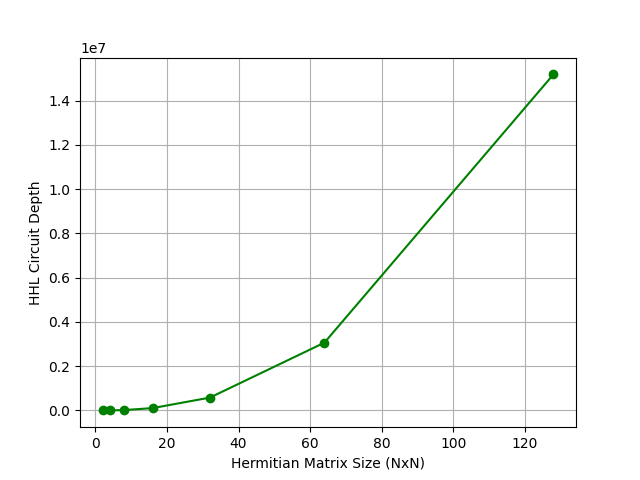
Figure 1: Quantum Circuit Depth vs. Ideal Matrix Size

But the number of problems that can be expressed as a linear system of equations is immense. It is possible that among the plethora of problems that can be expressed in this way, some are suitable to be solved through HHL.

Given the daily advances in quantum computing to handle depth, noise and quantum error correction, it is hard to set a limit to the parameters under which HHL’s implementation will be suitable. This paper proposes that given a certain depth threshold, matrices representing the linear system of equations can be classified as suitable or non-suitable for HHL through machine learning. As a proof of concept, this work trains and tests on a large number of linear systems of equations, and analyzes the impact of sparsity and condition numbers on the results. As a practical implementation, the approach is tested on the ability to solve the linear system of equations representing a single layer neural network to solve the classification of the IRIS dataset [Iris].

II HHL-Algorithm Implementation

Many problems can be reduced to solving a linear system of equations, and as such, HHL-based quantum acceleration has been a source of hope in many fields. As stated above, in quantum notation this linear system of equations is expressed as

$$A\ket{x}=\ket{b}$$ (4)

where $A$ is a Hermitian operator, and $\vec{b}$ has to be encoded in a quantum state $\ket{b}$ and, hence, it has to be normalized. Given a matrix $A$ of size $N\times N$, classical algorithms would have a computational complexity $O(N^{3})$. If the operator were expressed as a diagonal matrix, the calculation of $A^{-1}$ is almost immediate, creating a diagonal matrix in which the eigenvalues $\lambda_{i}$ in the diagonal are replaced by their corresponding inverted values, $\lambda_{i}^{-1}$. The computationally intensive portion of this solution in the classical context would be precisely to calculate the eigenvalues of $A$. This, however, can be solved rather easily in a quantum-mechanical manner through the use of the quantum phase estimation in which the eigenvalues are calculated and expressed as a phase.

$\ket{0}$ [label style=yshift=0.2cm]$\psi_{1}$ [4,steps=3,style=dashed,rounded corners,fill=green!20, inner xsep=2pt,background,label style=label position=below,anchor=north,yshift=-0.3cm]Loop until $\lambda$ sufficiently precise[label style=yshift=0.2cm]$\psi_{4}$ [3,disable auto height]λ^-1[label style=yshift=0.2cm]$\psi_{5}$ [label style=yshift=0.2cm]$\psi_{6}$
$\ket{0}$ n_ℓ [3,disable auto height]QPE [3,disable auto height]QPE^†
$\ket{0}$ n_a [label style=black,rotate=90, wires=2]Load —