SOReL and TOReL: Two Methods for Fully Offline Reinforcement Learning

Abstract

Sample efficiency remains a major obstacle for real world adoption of reinforcement learning (RL): success has been limited to settings where simulators provide access to essentially unlimited environment interactions, which in reality are typically costly or dangerous to obtain. Offline RL in principle offers a solution by exploiting offline data to learn a near-optimal policy before deployment. In practice, however, current offline RL methods rely on extensive online interactions for hyperparameter tuning, and have no reliable bound on their initial online performance. To address these two issues, we introduce two algorithms. Firstly, SOReL: an algorithm for safe offline reinforcement learning. Using only offline data our Bayesian approach infers a posterior over environment dynamics to obtain a reliable estimate of the online performance via the posterior predictive uncertainty. Crucially, all hyperparameters are also tuned fully offline. Secondly, we introduce TOReL: a tuning for offline reinforcement learning algorithm that extends our information rate based offline hyperparameter tuning methods to general offline RL approaches. Our empirical evaluation confirms SOReL’s ability to accurately estimate regret in the Bayesian setting whilst TOReL’s offline hyperparameter tuning achieves competitive performance with the best online hyperparameter tuning methods using only offline data. Thus, SOReL and TOReL make a significant step towards safe and reliable offline RL, unlocking the potential for RL in the real world. Our implementations are publicly available: https://github.com/CWibault/sorel_torel.

1 Introduction

Offline RL (Lange et al., 2012; Levine et al., 2020; Murphy, 2024) promises to unlock the potential for agents to act autonomously, successfully, and safely from the moment they are deployed into an environment. However, existing offline RL methods (Tarasov et al., 2023; Kostrikov et al., 2021; Kidambi et al., 2020; Yu et al., 2021) are yet to fulfil this promise; they require many online samples to carry out the extensive hyperparameter tuning required to achieve high performance (Zhang et al., 2021; Jackson et al., 2025), and there is no way of knowing whether the deployed policy will achieve good performance when initially deployed. Technically, current methods offer no reliable offline method to estimate true online regret, i.e. the difference between expected returns of an optimal policy and a policy trained using offline data. As we sketch in Fig.˜1(a), these factors result in cycles of training offline, deployment, failure online, further hyperparameter tuning, re-training offline and redeployment until the online performance of the agent is acceptable. Typically, online environment interactions are expensive, incorrect behaviour may be dangerous, and users need some guarantee of optimality within a fixed timeframe of deployment. This is concerning from an AI safety perspective, as without a reliable regret bound, we cannot deploy agents into the real world where agent failure presents a serious hazard to human life. In this paper, we develop two methods to address these two key issues of high online sample complexity and lack of online performance guarantees in offline RL.

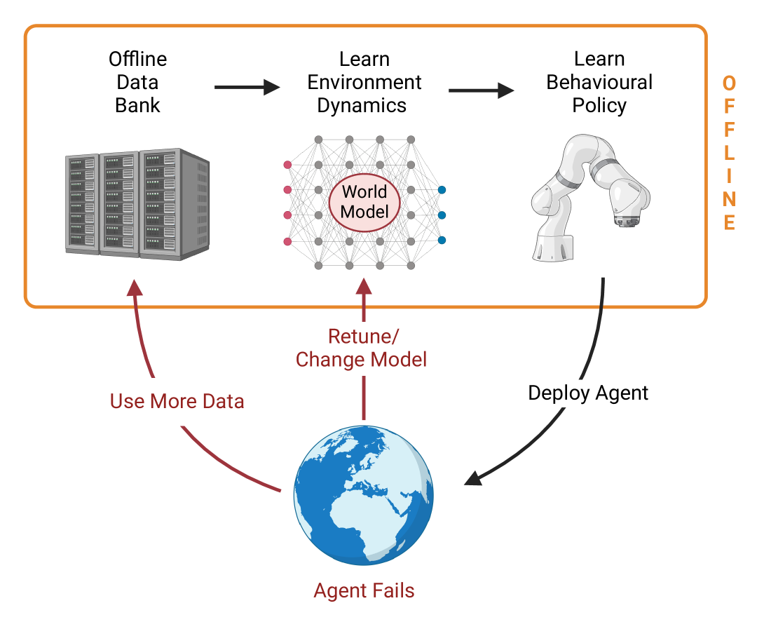
(a) Existing Model-Based Offline RL

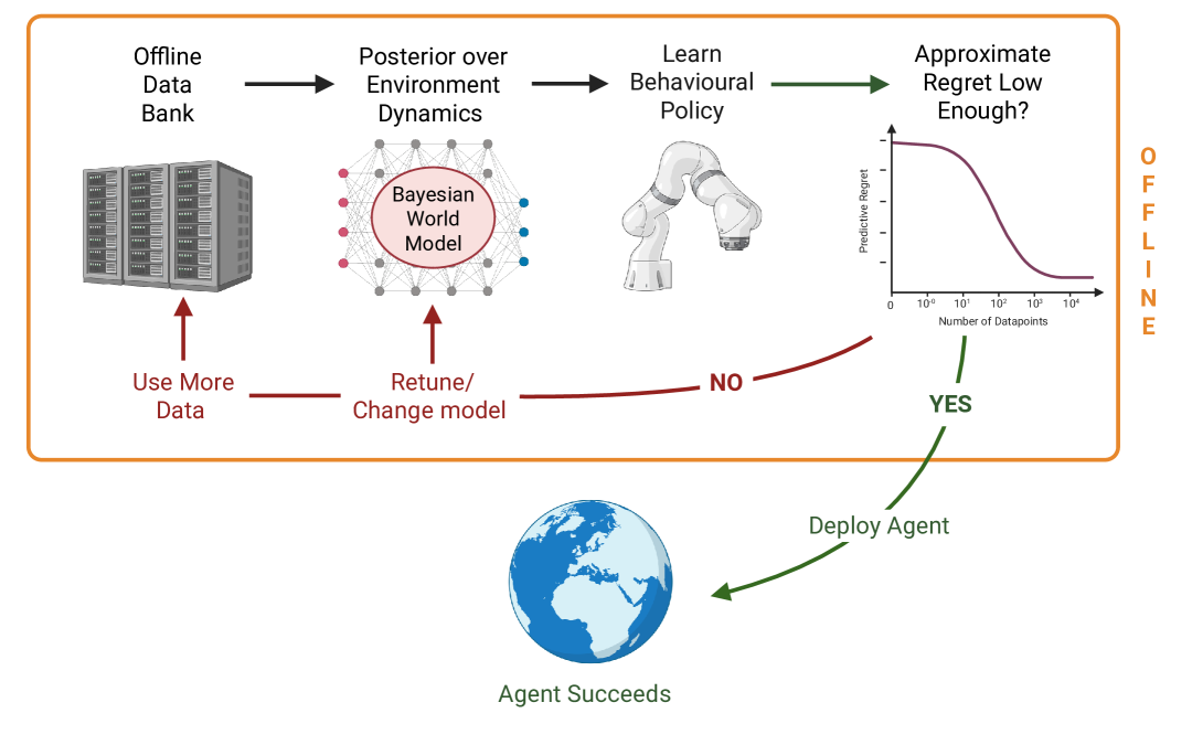
(b) SOReL (Our Approach)

Figure 1: Existing model-based offline approaches rely on online interactions for hyperparameter tuning and verifying accurate model learning before they can achieve good performance, leading to poor online sample efficiency. In contrast, in SOReL, model tuning and world model learning is carried out fully offline until a safe level of approximate regret is attained. Only then is the agent trained and deployed. Created in BioRender. Fellows, M. (2025) https://BioRender.com/gsdfdoz and https://BioRender.com/d3mgdw4

To address these issues, we develop a Bayesian framework where the posterior (conditioned on the offline data) is used as a prior for a Bayesian RL problem (Martin, 1967; Duff, 2002). Our analysis reveals that the regret of the corresponding Bayes-optimal policy is controlled by the posterior information loss (PIL) - that is the expected posterior KL divergence between the model and true dynamic. The change in PIL, known as the information rate, measures how much information the model has gained from an incremental amount of offline data. Crucially, the PIL can be estimated and tracked during offline training, allowing us to monitor performance and tune hyperparameters completely offline.

For our first method, we develop SOReL, a theoretically grounded framework for model-based safe offline reinforcement learning which tackles both key issues. Our analysis also reveals that by using offline data to infer a posterior over environment dynamics, we can approximate regret using the predictive variance and median of policy rollouts prior to deployment. As we show in Fig.˜1(b), if the PIL, and therefore regret is not falling fast enough, any issues involving hyperparameter tuning and model choice can be resolved offline. Only then is the trained agent deployed safely, making SOReL (to the authors’ knowledge) the first fully offline RL approach with reliable performance guarantees once deployed. Our first experiment supports this claim empirically, showing that in the standard offline RL MuJoCo control tasks (Yu et al., 2020; Kidambi et al., 2020; Ball et al., 2021; Lu et al., 2022b; Sun et al., 2023; Sims et al., 2024), SOReL’s offline regret approximation accurately tracks the true regret once deployed online.

For less conservative applications where accurate regret estimation is not required, we extend SOReL’s offline hyperparameter tuning methods to existing model-free and model-based offline RL approaches (Yu et al., 2020; Kidambi et al., 2020; Ball et al., 2021; Lu et al., 2022b; Sun et al., 2023; Tarasov et al., 2023; Sims et al., 2024). Using this insight, we develop TOReL, an algorithm for tuning offline reinforcement learning that tracks a regret metric correlated to the true regret. To test our method, we apply TOReL to IQL (Kostrikov et al., 2021), ReBRAC (Tarasov et al., 2023), MOPO (Yu et al., 2020) and MOReL (Kidambi et al., 2020) to carry out hyperparameter tuning in the standard offline RL MuJoCo control tasks. Using only offline data, TOReL achieves similar performance to existing methods that carry out online hyperparameter tuning. Notably, when combined with ReBRAC, TOReL consistently finds a hyperparameter combination with near-zero regret, outperforming all hyperparameters for all other algorithms. When comparing TOReL’s offline hyperparameter tuning to a recent online UCB approach (Jackson et al., 2025), we see that UCB typically requires about a dataset’s worth of online samples to match TOReL’s performance. We summarise our key contributions:

1. In Section˜4, we develop a Bayesian framework for model-based offline RL;

2. In Section˜5 we carry out a regret analysis for our framework, demonstrating regret is controlled by the PIL and providing a strong frequentist justification for our Bayesian approach;

3. In Section˜6.1 we develop SOReL, a method for approximating true regret using predictive uncertainty, which can achieve a desired and safe level of true regret once deployed;

4. In Section˜6.2 we introduce TOReL, adapting SOReL’s offline hyperparameter tuning approach to general offline model-based and model-free RL;

5. In Section˜7.1 we empirically confirm SOReL’s regret approximation as an accurate proxy for true regret;

6. In Section˜7.2, we also evaluate TOReL in the standard MuJoCo offline RL control tasks. Our approach achieves competitive performance with the best online hyperparameter tuning methods using only offline data, and achieving near-zero regret when combined with ReBRAC.

2 Preliminaries

2.1 Mathematical Notation

Let $X$ be a $\mathcal{X}\subseteq\mathbb{R}^{n}$-valued random variable. We denote a distribution as $P_{X}$ with density (if it exists) as $p(x)$. We denote the set of all distributions over $\mathcal{X}$ as $\mathcal{P}(\mathcal{X})$. We introduce the notation $\mathcal{G}(p)$ to represent the geometric distribution and $\mathcal{AG}(p)$ to represent the arithmetico-geometric distribution, with probability mass functions: $P_{\mathcal{G}}(i)\coloneqq(1-p)p^{i}$ and $P_{\mathcal{AG}}(i)\coloneqq(1-p)^{2}p^{i}(i+1)$ respectively, for $i\in\mathbb{N}_{0}^{+}$ and parameter $p\in[0,1)$. We denote the uniform distribution over $\{0,1,\dots i\}$ as $\mathcal{U}_{i}$ and the multivariate normal distribution with mean vector $\mu$ and covariance matrix $\Sigma$ as $\mathcal{N}(\mu,\Sigma)$.

2.2 Offline Reinforcement Learning

For our offline RL setting, an agent is tasked with solving the learning problem in an infinite-horizon, discounted Markov decision process (Bellman, 1956, 1958; Sutton and Barto, 2018; Puterman, 1994; Szepesvári, 2010): $\mathcal{M}^{\star}\coloneqq\langle\mathcal{S},\mathcal{A},P_{0},P_{S}^{\star}(s,a),P_{R}^{\star}(s,a),\gamma\rangle,$ with state space $\mathcal{S}$, action space $\mathcal{A}$ and discount factor $\gamma$. At time $t=0$, an agent starts in an initial state allocated according the the initial state distribution: $s_{0}\sim P_{0}$. At every timestep $t$, an agent in state $s_{t}$ takes an action according to a policy $a_{t}\sim\pi(h_{t})$, receives a scalar reward $r_{t}\sim P_{R}^{\star}(s_{t},a_{t})$ and transitions to a new state $s_{t+1}\sim P_{S}^{\star}(s_{t},a_{t})$ where $h_{t}\coloneqq\{s_{0},a_{0},r_{0},s_{1},a_{1},r_{1},\ldots a_{t-1},r_{t-1},s_{t}\}\in\mathcal{H}_{t}$ is the observed a history of interactions with the environment. Here $\mathcal{H}_{t}\coloneqq\mathcal{S}\times(\mathcal{A}\times\mathbb{R}\times\mathcal{S})^{\times t}$ denotes the corresponding product space. We assume rewards are bounded with $r_{t}\in[r_{\textrm{min}},r_{\textrm{max}}]\subset\mathbb{R}$ where $r_{\textrm{min}}$ and $r_{\textrm{max}}$ denote the minimum and maximum reward values respectively. For convenience, we often write the joint state transition-reward distribution as $P_{R,S}^{\star}(s,a)$. We denote the distribution over history $h_{t}$ as $P^{\star}_{t,\pi}$. The goal of an agent is to learn an optimal policy $\pi^{\star}\in\Pi^{\star}$ where $\Pi^{\star}\coloneqq\operatorname*{arg\,max}_{\pi}J^{\pi}(\mathcal{M}^{\star})$ is the set of policies that maximise the expected discounted return $J^{\pi}(\mathcal{M}^{\star}):=\mathbb{E}_{h_{\infty}\sim P^{\star}_{\infty,\pi}}\left[\sum_{i=0}^{\infty}\gamma^{i}r_{i}\right]$. It suffices to consider only optimal policies that condition only on the most recent state (i.e. $\pi^{\star}(s_{t})$) as, in a fully observable MDP, any optimal history-conditioned policy will never take an action that cannot be taken by an optimal policy that conditions only on most recent state.

In the learning setting, the true state transition distribution $P_{S}^{\star}(s,a)$ and reward distribution $P_{R}^{\star}(s,a)$ are assumed unknown a priori. Once deployed, the agent is faced with the exploration/exploitation dilemma in that it must balance exploring to learn about the unknown environment dynamics with exploiting. In offline RL (Lange et al., 2012; Levine et al., 2020; Murphy, 2024), an agent has access to a dataset of histories of various lengths collected from the true environment. The policies used to collect the data may vary and not be optimal. In the zero-shot model-based offline RL setting (Jackson et al., 2025), the dataset is used to learn the unknown environment dynamics from which a policy is trained prior to any interaction with the environment. The agent is then deployed at test time $t=0$ and its performance evaluated. The goal of offline RL is to take advantage of offline data so that the deployed policy will be near-optimal from the outset.

3 Related Work

Developing reliable model-based offline RL algorithms remains an open challenge for several reasons. In addition to our key issues of high online sample complexity and lack of online performance guarantees, $i)$ the performance of approaches is particularly dependent on the ability to accurately model transition dynamics as errors in a dynamics model can compound over several timesteps for the long-horizon problems encountered in RL (see also our analysis in Section˜5.2); $ii)$ many datasets used to benchmark methods contain missing datapoints in critical regions of state-action space, which poses an additional orthogonal generalisation challenge. Most existing offline RL methods focus on tackling issue $ii)$ by introducing a form of reward pessimism based on the model uncertainty (Yu et al., 2020; Kidambi et al., 2020; Kumar et al., 2020; Yu et al., 2021; Fujimoto and Gu, 2021; Kostrikov et al., 2021; An et al., 2021; Ball et al., 2021; Lu et al., 2022b; Sun et al., 2023; Tarasov et al., 2023; Sims et al., 2024). Unifloral (Jackson et al., 2025) is a recent framework that unites these offline RL approaches into a single algorithmic space with lightweight and high-performing implementations, as well as providing a clarifying benchmarking protocol. Our implementations and evaluation methods follow this framework.

Only limited attention has been given to the two aforementioned issues of high online sample complexity and lack of performance guarantees: Paine et al. (2020) introduce a method for estimating online value and partial hyperparameter tuning of offline model-free algorithms, however their method neither approximates regret, nor is an accurate proxy for true value, resulting in significant overestimation in most domains. As noted by Smith et al. (2023), their approach relies on offline policy evaluation, which is a challenging and provably difficult problem (Wang et al., 2020) whose hyperparameters require tuning online. Moreover, as noted by Jackson et al. (2025), their framework is limited to behavioural cloning and two model-free critic-based methods that have since been outperformed by modern algorithms. Smith et al. (2023) introduce a method for offline hyperparameter tuning, but are limited to the model-free imitation learning setting and offer no regret estimation. Finally, Wang et al. (2022) introduce a method for offline hyperparameter tuning to pre-select hyperparameters for online methods, but do not learn optimal policies offline or provide regret approximation. In contrast to all of these approaches, to the authors’ knowledge, our method is the first offline RL method to reliably approximate regret and carry out all hyperparameter tuning for general methods using only offline data. Finally, understanding of offline RL from a Bayesian perspective is limited. To the authors’ knowledge, only Chen et al. (2024) have framed solving offline model-based RL as solving a BAMDP, however no regret analysis of the Bayes-optimal policy is carried out, a continuous BAMCP (Guez et al., 2014) approximation is used to learn behavioural policies and the algorithm still suffers from a lack of regret approximation, hence relying on online data for tuning and data integration.

4 Bayesian Offline RL

We now introduce our framework for safe offline RL (SOReL), which constitutes first learning an (approximate) posterior from offline data before solving a Bayesian RL problem with the posterior acting as the prior. We provide an introductory primer on Bayesian RL in Appendix˜B.

4.1 Learning a Posterior with Offline Data

A Bayesian epistemology characterises the agent’s uncertainty in the MDP through distributions over any unknown variable (Martin, 1967; Duff, 2002). We first specify a parametric model $p(r_{t},s_{t+1}|s_{t},a_{t},\theta)$, $P_{R,S}(s_{t},a_{t},\theta)$, $\theta\in\Theta\subset\mathbb{R}^{d}$, over the unknown state transitions and reward distributions, with each $\theta\in\Theta\subseteq\mathbb{R}^{d}$ representing a hypothesis about the MDP $\mathcal{M}^{\star}$. As we show in Section˜5.1, our results can easily be generalised to non-parametric methods like Gaussian process regression (Rasmussen and Williams, 2006; Wiener, 1923; Krige, 1951). A prior distribution over the parameter space $P_{\Theta}$ is specified, which represents the initial a priori belief in the true value of $P_{R,S}^{\star}(s,a)$ before the agent has observed any transitions.

We denote an offline dataset of $N$ state-action-state-reward transition observations as: $\mathcal{D}_{N}=\{(s_{i},a_{i},s^{\prime}_{i},r_{i})\}_{i=0}^{N-1}$, all collected from a single MDP $\mathcal{M}^{\star}$. Datapoints may be collected from several policies and non-Markovian sampling. Given the dataset $\mathcal{D}_{N}$, the prior $P_{\Theta}$ with density $p(\theta)$ is updated to posterior $P_{\Theta}(\mathcal{D}_{N})$ with density $p(\theta|\mathcal{D}_{N})$, using Bayes’ rule:

$$p(\theta|\mathcal{D}_{N})=\frac{p(\mathcal{D}_{N}|\theta)p(\theta)}{p(\mathcal{D}_{N})}=\frac{\prod_{i=0}^{N-1}p(r_{i},s_{i}^{\prime}|s_{i},a_{i},\theta)p(\theta)}{\int_{\Theta}\prod_{i=0}^{N-1}p(r_{i},s_{i}^{\prime}|s_{i},a_{i},\theta)p(\theta)d\theta}.$$ (1)

The posterior represents the agent’s belief in the unknown environment dynamics once $\mathcal{D}_{N}$ has been observed. We now detail how a Bayes-optimal policy is learned using the posterior as the initial belief in the environment dynamics.

4.2 Learning a Bayes-optimal Policy

It is well known that solving a Bayesian RL problem exactly is intractable for all but the simplest models (Martin, 1967; Duff, 2002; Guez et al., 2012, 2013; Zintgraf et al., 2020; Fellows et al., 2024). Inferring the posterior in Eq.˜1 is typically infeasible for dynamics models of interest (for example, nonlinear Gaussian world models). This is because there is no analytic solution for the posterior density and the cost of carrying out integration required to evaluate the evidence $p(\mathcal{D}_{N})$ grows exponentially in parameter dimensions $d$. Fortunately, there exist tractable methods to learn an approximate posterior $\hat{P}_{\Theta}(\mathcal{D}_{N})\approx P_{\Theta}(\mathcal{D}_{N})$; in this paper we use randomised priors (Osband and Van Roy, 2017; Osband et al., 2018; Ciosek et al., 2020) (RP) and provide details in Section˜F.2. In addition, a planning problem must be solved for every conceivable history that an agent could encounter. In our offline RL setting, we ease intractability by replacing the prior $P_{\Theta}$ with a highly informative posterior $P_{\Theta}(\mathcal{D}_{N})$, significantly reducing the hypothesis space in the Bayesian RL problem.

Let $P_{\infty,\pi}(\theta)$ denote the corresponding model distribution over $h_{\infty}$ for policy $\pi(h_{t})$. To obtain an (approximately) Bayes-optimal policy, we use the Bayesian RL objective in the meta-learning form (Zintgraf et al., 2020; Beck et al., 2024) (i.e. as an expectation using $\hat{P}_{\Theta}(\mathcal{D}_{N})$) so that a simple RL²(Duan et al., 1987) style algorithm can be applied:

$$J^{\pi}_{\textrm{Bayes}}(\hat{P}_{\Theta}(\mathcal{D}_{N}))\coloneqq\mathbb{E}_{\theta\sim\hat{P}_{\Theta}(\mathcal{D}_{N})}\left[\mathbb{E}_{h_{\infty}\sim P_{\infty,\pi}(\theta)}\left[\sum_{i=0}^{\infty}\gamma^{i}r_{i}\right]\right].$$ (2)

Solving Eq.˜2 is known as solving a Bayes-adaptive MDP (BAMDP) (Duff, 2002). We optimise the objective in Eq.˜2 by sampling a hypothesis environment from the approximate posterior $\theta\sim\hat{P}_{\Theta}(\mathcal{D}_{N})$ then rolling out the policy in the sampled environment dynamics. The Bayes-optimal policy $\pi^{\star}_{\textrm{Bayes}}\in\operatorname*{arg\,max}_{\pi}J^{\pi}_{\textrm{Bayes}}(\hat{P}_{\Theta}(\mathcal{D}_{N}))$ is learned using RNN-PPO (Schulman et al., 2017) as a BAMDP solver on the rollouts. Complete implementation details can be found in Appendix˜F.

In addition to having excellent exploration/exploitation properties, a Bayesian approach affords access to epistemic uncertainty in the returns via the variance of predictive rollouts. Uncertainty estimation is essential for tackling our two keys issues; firstly, as we show in Section˜7.1, the predictive variance and predictive median of policy returns can be used to estimate the true regret at test time. Secondly, monitoring the decay of predictive variance and regret is a powerful tool for diagnosing issues offline; if not decaying, the practitioner can fix any issues with model choice, hyperparameter tuning or the prior $P_{\Theta}$ before deployment, eliminating the need for online samples. Finally, we remark that a Bayesian approach is relatively simple compared to existing model-based approaches in Section˜3 as it does not rely on hand-crafted heuristics tailored to specific problem settings.

5 Regret Analysis

We carry out a frequentist regret analysis for Bayesian offline RL. The goal of this analysis is to characterise how the rate of regret decreases for a Bayes-optimal policy using an easy to estimate quantity known as the posterior information loss (PIL). All proofs for all theorems can be found in Appendix˜D.

5.1 Controlling Regret with the PIL

For ease of exposition, we assume the real MDP is parametrised by some $\theta^{\star}\in\Theta$. According to the Bernstein-von Mises theorem (Doob, 1949; Le Cam, 1953; Vaart, 1998), as the posterior becomes more informative it concentrates around a smaller (and more tractable) subset of hypothesis space $\Theta$ centred on $\theta^{\star}$. Not only does this ease the computational burden of solving the BRL objective in Eq.˜2, but in the limit $N\rightarrow\infty$, the Bayesian RL objective using the true posterior from Eq.˜2 will approach the true expected discounted return for the MDP: $J^{\pi}(P_{\Theta}(\mathcal{D}_{N}))\xrightarrow[N\rightarrow\infty]{}J^{\pi}(\mathcal{M}^{\star})$. In this limit, any Bayes-optimal policy will be an optimal policy for the true MDP, achieving the highest expected returns once deployed. For finite $N$, we can measure how far the performance of the Bayes optimal policy is from an optimal policy using the true regret, which is the difference between the expected return $J^{\pi_{\textrm{Bayes}}^{\star}}(\mathcal{M}^{\star},\mathcal{D}_{N})$ of the Bayes-optimal policy $\pi_{\textrm{Bayes}}^{\star}$ given a posterior $P_{\Theta}(\mathcal{D}_{N})$, all in the true MDP $\mathcal{M}^{\star}$:

$$\textnormal{{Regret}}(\mathcal{M}^{\star},\mathcal{D}_{N})\coloneqq J^{\pi^{\star}}(\mathcal{M}^{\star})-J^{\pi_{\textrm{Bayes}}^{\star}}(\mathcal{M}^{\star},\mathcal{D}_{N}).$$ (3)

Accurately approximating true regret is challenging and exact calculation is impossible unless the true environment dynamics $\mathcal{M}^{\star}$ are known. To make progress towards approximating regret, we bound it using the PIL, defined as:

$$\mathcal{I}_{N}^{\pi}\coloneqq \mathbb{E}_{\theta\sim P_{\Theta}(\mathcal{D}_{N})}\left[\mathbb{E}_{s,a\sim\rho_{\pi}^{\star}}\left[\textrm{KL}\left(P_{R,S}^{\star}(s,a)\|P_{R,S}(s,a,\theta)\right)\right]\right].$$ (4)

Here $\rho_{\pi}^{\star}\coloneqq\mathbb{E}_{i\sim\mathcal{AG(\gamma)}}\left[\mathbb{E}_{j\sim\mathcal{U}_{i}}\left[P_{j,\pi}^{\star}\right]\right]$ is the arithemetico-geometric ergodic state-action distribution, which places mass over state-action pairs according to how much errors in the model influence the regret at each state. Regions of state-action space that require more timesteps to reach from initial states are weighted significantly less than those that are encountered earlier and more frequently, as state errors encountered early accumulate in each prediction from that timestep onwards.

The PIL has an intuitive information-geometric interpretation: the inner expectation $\mathbb{E}_{s,a\sim\rho_{\pi}^{\star}}\left[\textrm{KL}\left(P_{R,S}^{\star}(s,a)\|P_{R,S}(s,a,\theta)\right)\right]$ measures the distance between the model and the true distribution in terms of the information lost when approximating $P_{R,S}^{\star}(s,a)$ with $P_{R,S}(s,a,\theta)$, averaged across all states. The PIL thus measures how close the posterior’s belief is to the truth according to the average information lost under the posterior expectation. We observe that via Jensen’s inequality, the PIL is an upper bound on the classic KL risk (sometimes known as expected relative entropy) from Bayesian asymptotics and regret analysis (Aitchison, 1975; Clarke and Barron, 1990; KOMAKI, 1996; Hartigan, 1998; Barron, 1988, 1999; Yang and Barron, 1999; van der Vaart and van Zanten, 2011; Aslan, 2006; Alaa and van der Schaar, 2018; Bilodeau et al., 2021).

Theorem 1.

Let $\mathcal{R}_{\max}\coloneqq\frac{(r_{\textrm{max}}-r_{\textrm{min}})}{1-\gamma}$ denote the maximum possible regret for the MDP. Using the posterior information distance in Eq.˜4, the true regret is bounded as:

$$\textnormal{{Regret}}(\mathcal{M}^{\star},\mathcal{D}_{N})\leq 2\mathcal{R}_{\max}\cdot\sup_{\pi}\sqrt{1-\exp\left(-\frac{\mathcal{I}_{N}^{\pi}}{1-\gamma}\right)}$$ (5)

From Ineq. 5, we observe that the rate at which regret decreases with $N$ is governed by the rate at which the PIL decreases, which is known as the information rate, which measures how much information the model has gained from an incremental amount of data. Fast information rates imply highly informative posteriors can be learned using minimal data as regret will decrease at least as fast. How fast the information rate is depends on the exact model specification, prior and underlying MDP. Formulating our bound in terms of the PIL ties the regret to the KL divergence over the reward-state model: $\textrm{KL}\left(P_{R,S}^{\star}(s,a)\|P_{R,S}(s,a,\mathcal{D}_{N})\right)$. Not only is this mathematically more convenient, yielding a simpler bound, but the PIL is easy to estimate in practice meaning the information rate can be monitored offline to gauge online performance and carry out hyperparameter tuning. We observe that our results in Theorem˜1 also apply for offline frequentist settings where an estimate, e.g. the maximum likelihood estimate $\hat{\theta}_{N}^{\textrm{MLE}}\coloneqq\operatorname*{arg\,max}_{\theta}\log p(\mathcal{D}_{N}|\theta)$, is calculated from the dataset $\mathcal{D}_{N}$. Here, the posterior is replaced with the point estimate $P_{\Theta}(\mathcal{D}_{N})=\delta(\theta=\hat{\theta}_{N}^{\textrm{MLE}})$.

5.2 Frequentist Justification for Bayesian Offline RL

Using Theorem˜1, we can study the PIL $\mathcal{I}^{\pi}_{N}$ for different classes of models which allows us to understand how regret will evolve given the model choice. This also provides a frequentist justification for many Bayesian approaches. We now characterise the information rate for parametric models.

Theorem 2.

Let the data be drawn from the underlying true distribution $\mathcal{D}_{N}\sim P_{\textrm{Data}}^{\star}$. Under standard local asymptotic normality assumptions (see ˜1 in Section˜D.3), there exists some constant $0<C<\infty$ such that for sufficiently large $N$:

$$\mathbb{E}_{\mathcal{D}_{N}\sim P_{\textrm{Data}}^{\star}}\left[\textnormal{{Regret}}(\mathcal{M}^{\star},\mathcal{D}_{N})\right]\leq 2\mathcal{R}_{\max}\cdot\exp\left(1-\sqrt{\frac{Cd}{(1-\gamma)N}}\right).$$ (6)

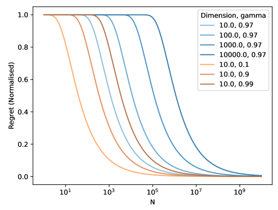
Figure 2: Normalised Regret Curves for $C=1$

Theorem˜2 applies to the Gaussian world model introduced in Section˜5.3 with neural network mean functions with $C^{2}$-continuous activations (tanh, identity, sigmoid, softplus, SiLU, SELU, GELU…) using a Gaussian or uniform prior truncated to a compact parameter space and similarly well-behaved parametric models. The $\mathcal{O}\left(\nicefrac{{d}}{{N}}\right)$ information rate coincides with the optimal ‘minimax’ convergence rate of frequentist parametric density estimators (Yang and Barron, 1999; Bilodeau et al., 2021), providing a strong frequentist justification for our Bayesian offline RL framework. The resulting differences in performance only arise from the choice of prior, model representability and coverage of dataset, which affect Bayesian and frequentist methods equally. Similar results for the information rate have been found for nonparametric models such a Gaussian processes (van der Vaart and van Zanten, 2011). We note that the bound in Ineq 6 is upper bounded as $\mathcal{O}\left(\sqrt{\nicefrac{{d}}{{N}}}\right)$, which relates our method to regret rates found in prior work (Yu et al., 2020; Kidambi et al., 2020).

Using our result in Theorem˜2, we plot the normalised regret bound (i.e. taking $\mathcal{R}_{\max}=0.5$) in Ineq. 6 for increasing dimensionality (blue) and decreasing $\gamma$ (copper) in Fig.˜2. Our bound reveals an S-shaped curve with three distinct phases as number of data points $N$ increases: an initial plateau, a sudden decrease in regret follow by a slow exponential decay towards a regret of zero. The plateau indicates that a minimum amount of data is needed before any benefit can be realised in terms of regret. This is to be expected because initially the only information about the parameter values is given by the prior, which has no guarantee of accuracy under our analysis. Once a threshold of data points has been reached, the data can start to overwhelm the prior, resulting in a sudden decrease in regret. The higher the dimensionality of the model, the greater this data limit is - represented in Fig.˜2 by the plateau length increasing with greater $d$ (blue curves). Due to overspecification in models, this limit is likely to be set by the effective dimension of the problem (which may be much lower than $d$) as many parameters will be redundant, however the effective dimension is typically not possible to ascertain a priori. Finally, we observe that increasing the discount factor $\gamma$ leads to a longer regret plateau (copper curves) due to any error in the model dynamics being compounded over a longer horizon at test time.

5.3 Gaussian World Models

Many methods specify Gaussian reward and state transition models of the form:

$$P_{R}(s,a,\theta)=\mathcal{N}(r_{\theta}(s,a),\sigma^{2}_{r}(s,a)),\quad P_{S}(s,a,\theta)=\mathcal{N}(s^{\prime}_{\theta}(s,a),I\sigma^{2}_{s}(s,a)),$$ (7)

with isotropic variance characterised by $\sigma^{2}_{r}$ and $\sigma^{2}_{s}$, mean reward function $r_{\theta}(s,a)$ and mean state transition function $s^{\prime}_{\theta}(s,a)$. Using a Gaussian world model, we find the PIL takes a convenient and intuitive form. Let $r(s,a,\mathcal{D}_{N})\coloneqq\mathbb{E}_{\theta\sim P_{\Theta}(\mathcal{D}_{N})}\left[r_{\theta}(s,a)\right]$ and $s^{\prime}(s,a,\mathcal{D}_{N})\coloneqq\mathbb{E}_{\theta\sim P_{\Theta}(\mathcal{D}_{N})}\left[s_{\theta}(s,a)\right]$ denote the Bayesian mean reward and state transition functions and $r^{\star}(s,a)$ and ${s^{\star}}^{\prime}(s,a)$ denote the true mean functions. We define the mean squared error between the true and Bayesian mean functions as:

$$\mathcal{E}(\mathcal{D}_{N},\mathcal{M}^{\star})\coloneqq\mathbb{E}_{(s,a)\sim\rho_{\pi}^{\star}}\left[\frac{\lVert r(s,a,\mathcal{D}_{N})-r^{\star}(s,a)\rVert^{2}_{2}}{2\sigma_{r}^{2}(s,a)}+\frac{\lVert s^{\prime}(s,a,\mathcal{D}_{N})-{s^{\star}}^{\prime}(s,a)\rVert^{2}_{2}}{2\sigma_{s}^{2}(s,a)}\right],$$ (8)

and the predictive variance as:

$$\mathcal{V}(\mathcal{D}_{N})\coloneqq\mathbb{E}_{(s,a)\sim\rho_{\pi}^{\star}}\left[\mathbb{E}_{\theta\sim P_{\Theta}(\mathcal{D}_{N})}\left[\frac{\lVert r(s,a,\mathcal{D}_{N})-r_{\theta}(s,a)\rVert^{2}_{2}}{2\sigma_{r,}^{2}(s,a)}+\frac{\lVert s^{\prime}(s,a,\mathcal{D}_{N})-s^{\prime}_{\theta}(s,a)\rVert^{2}_{2}}{2\sigma_{s}^{2}(s,a)}\right]\right].$$ (9)

We now re-write the PIL for the Gaussian world model using these two terms:

Proposition 1.

Using the Gaussian world model in Eq.˜7, it follows:

$$\mathcal{I}_{N}^{\pi}=\mathcal{E}(\mathcal{D}_{N},\mathcal{M}^{\star})+\mathcal{V}(\mathcal{D}_{N}).$$ (10)

Eq.˜10 shows that the PIL is governed by i) the mean squared error of the point estimate $\mathcal{E}(\mathcal{D}_{N},\mathcal{M}^{\star})$, which characterises how quickly the Bayesian mean function converges to the true function; and ii) the predictive variance $\mathcal{V}(\mathcal{D}_{N})$, which characterises the epistemic uncertainty in the model. For frequentist methods using point estimates like the MLE, there is no characterisation of epistemic uncertainty, meaning $\mathcal{V}(\mathcal{D}_{N})=0$. The PIL can easily be estimated by estimating $\mathcal{E}(\mathcal{D}_{N},\mathcal{M}^{\star})$ using the empirical MSE with offline data and estimating $\mathcal{V}(\mathcal{D}_{N})$ using posterior sampling.

6 From Theory to Practice

Our frequentist analysis in Section˜5 provides valuable intuition about how we might expect regret to change depending on the choice of model, however it cannot address the two key issues of online sample efficiency and performance guarantees from Section˜1. This is because it cannot provide a precise answer to questions like ‘what will the regret of the deployed policy be?’ or ‘which hyperparameter has the lowest regret?’ as the results depend on constants that condition on $\mathcal{M}^{\star}$, which is unknown a priori, and are characterised in terms of asymptotic limits of large data, often relying on $N$ being large enough with little qualification of what large enough means. These issues stem from the fact that a purely frequentist regret analysis treats the unknown distribution as true and data as random, thereby violating the conditionality principle (Birnbaum, 1962; Gandenberger, 2015). Our Bayesian approach can bypass this issue, allowing for offline regret approximation and hyperparameter tuning by monitoring the PIL and predictive median and variance, which only condition on observed data.

6.1 SOReL

We now introduce SOReL in Algorithm˜1, our algorithm for reliable regret estimation and offline hyperparameter tuning. In our SOReL framework, there are three sets of hyperparameters: $\phi_{I}$ the model (such as the architecture for a neural-network function approximator); $\phi_{II}$ the approximate inference method (such as the number of ensemble members for RP); and $\phi_{III}$ the BAMDP solver (the hyper-parameters of a Bayesian meta-learning algorithm like RNN-PPO). Sets $\phi_{I}$ and $\phi_{II}$ are tuned jointly to both minimise the PIL and ensure a roughly even split between the predictive variance and MSE loss terms. Set $\phi_{III}$ is then tuned to minimise approximate regret based on the now-fixed model and approximate posterior: for each combination of hyper-parameters, we learn a policy using the BAMDP solver, and choose the combination whose policy leads to the lowest approximate regret. $\mathcal{R}_{\textrm{Deploy}}$ denotes the desired level of regret of the deployed policy.

Regret Approximation: A simple approach for bounding regret would be to estimate the PIL from the offline data using Eq.˜10 and then apply our theoretical upper bound in Eq.˜5. This is likely to be too conservative for most applications as it protects against the worst case MDP that the agent could encounter. In particular, it is very sensitive to errors in the model, especially as $\gamma\rightarrow 1$, which is an artifact of model errors accumulating over all future timesteps in the regret analysis. Instead, we approximate the regret using the posterior predictive median:

$$\textnormal{{Regret}}(\mathcal{M}^{\star},\mathcal{D}_{N}) \approx\hat{R}_{\max}-\hat{\mathbb{M}}_{\theta\sim P_{\Theta}(\mathcal{D}_{N}),h_{\infty}\sim P_{\infty}^{\pi}(\theta)}\left[R(h_{\infty})\right],$$ (11)

Algorithm 1 SOReL$(P_{\Theta},\mathcal{D}_{N},\mathcal{R}_{\textrm{Deploy}})$

$R_{N}\leftarrow\hat{\mathcal{R}}_{\max}$

while $R_{N}>\mathcal{R}_{\textrm{Deploy}}$ do

  Hyperparameter tuning:

  $\textrm{{\color[rgb]{0.59,0,0.66}$\phi_{I}$}},\textrm{{\color[rgb]{0,0.6,0}$\phi_{II}$}}\leftarrow\operatorname*{arg\,min}_{\textrm{{\color[rgb]{0.59,0,0.66}$\phi_{I}$}},\textrm{{\color[rgb]{0,0.6,0}$\phi_{II}$}}}\textrm{PIL}(\textrm{{\color[rgb]{0.59,0,0.66}$\phi_{I}$}},\textrm{{\color[rgb]{0,0.6,0}$\phi_{II}$}},\mathcal{D}_{N})$

   $\text{ s.t. }\mathcal{E}(\mathcal{D}_{N},\mathcal{M}^{\star})\approx\mathcal{V}(\mathcal{D}_{N})$

  $\textrm{{\color[rgb]{1,0.23,0.13}$\phi_{III}$}}\leftarrow\operatorname*{arg\,min}_{\textrm{{\color[rgb]{1,0.23,0.13}$\phi_{III}$}}}\text{ApproxRegret}(\textrm{{\color[rgb]{0.59,0,0.66}$\phi_{I}$}},\textrm{{\color[rgb]{0,0.6,0}$\phi_{II}$}},\textrm{{\color[rgb]{1,0.23,0.13}$\phi_{III}$}},\mathcal{D}_{N})$

  Policy Learning and Regret Approximation:

  $\pi^{\star}_{\textrm{Bayes}}\leftarrow\textrm{SolveBAMDP}(\textrm{{\color[rgb]{0.59,0,0.66}$\phi_{I}$}},\textrm{{\color[rgb]{0,0.6,0}$\phi_{II}$}},\textrm{{\color[rgb]{1,0.23,0.13}$\phi_{III}$}},\mathcal{D}_{N})$

  $R_{N}\leftarrow\text{ApproxRegret}(\textrm{{\color[rgb]{0.59,0,0.66}$\phi_{I}$}},\textrm{{\color[rgb]{0,0.6,0}$\phi_{II}$}},\textrm{{\color[rgb]{1,0.23,0.13}$\phi_{III}$}},\mathcal{D}_{N})$

end while

return $\pi^{\star}_{\textrm{Bayes}}$

where $\hat{\mathbb{M}}_{\theta\sim P_{\Theta}(\mathcal{D}_{N}),h_{\infty}\sim P_{\infty}^{\pi}(\theta)}\left[R(h_{\infty})\right]$ denotes the median predictive return based on sampling from the (approximate) posterior and rolling out the Bayes-optimal policy and $\hat{R}_{\max}$ is estimated from the maximum return in the offline dataset - full details and an overview of alternative metrics that can be derived from the posterior to approximate the regret with varying degrees of conservatism are found in Section˜C.2. We hypothesise that the sample median offers a good compromise: neither overly conservative nor overly susceptible to being skewed by a policy that performs well on only a subset of posterior samples. Our empirical evaluations support this hypothesis in Section˜7.1. The posterior predictive median also allows us to tune hyperparameter set $\phi_{III}$, selecting hyperparameters to learn a policy that achieves the lowest approximate regret as shown in Algorithm˜1.

Information Rate Monitoring: To tune sets $\phi_{I}$ and $\phi_{II}$, we monitor the information rate (recall, the change in PIL defined in Eq.˜4). Our goal is to select hyperparameters that minimises the PIL whilst ensuring the the MSE term (c.f. Eq.˜8) closely matches the predictive variance term (c.f. Eq.˜9): $\mathcal{E}(\mathcal{D}_{N},\mathcal{M}^{\star})\approx\mathcal{V}(\mathcal{D}_{N})$. Misalignment of predictive variance and MSE indicates either an overfitting/underfitting issue with model hyperparameters in set $\phi_{I}$ and/or an issue with uncertainty estimation due to approximate inference hyperparameters in set $\phi_{II}$. Moreover, under/overestimating uncertainty will lead to poor regret estimation, which is why we tune sets $\phi_{I}$ and $\phi_{II}$ first in Algorithm˜1. Our empirical evaluations in Section˜7.1 confirm that when $\mathcal{E}(\mathcal{D}_{N},\mathcal{M}^{\star})\approx\mathcal{V}(\mathcal{D}_{N})$, the approximate regret aligns strongly with true regret.

Algorithm 2 TOReL$(P_{\Theta},\mathcal{D}_{N})$

$\textrm{{\color[rgb]{0.59,0,0.66}$\phi_{I}$}},\textrm{{\color[rgb]{0,0.6,0}$\phi_{II}$}}\leftarrow\operatorname*{arg\,min}_{\textrm{{\color[rgb]{0.59,0,0.66}$\phi_{I}$}},\textrm{{\color[rgb]{0,0.6,0}$\phi_{II}$}}}\textrm{PIL}(\textrm{{\color[rgb]{0.59,0,0.66}$\phi_{I}$}},\textrm{{\color[rgb]{0,0.6,0}$\phi_{II}$}},\mathcal{D}_{N})$

 $[\text{ s.t. }\mathcal{E}(\mathcal{D}_{N},\mathcal{M}^{\star})\approx\mathcal{V}(\mathcal{D}_{N}),(\text{model-based})]$

$\textrm{{\color[rgb]{1,0.23,0.13}$\phi_{III}$}}\leftarrow\operatorname*{arg\,min}_{\textrm{{\color[rgb]{1,0.23,0.13}$\phi_{III}$}}}\text{RegretMetric}(\textrm{{\color[rgb]{0.59,0,0.66}$\phi_{I}$}},\textrm{{\color[rgb]{0,0.6,0}$\phi_{II}$}},\textrm{{\color[rgb]{1,0.23,0.13}$\phi_{III}$}},\mathcal{D}_{N})$

$\pi^{\star}_{\textrm{TOReL}}\leftarrow\begin{cases}\textrm{ORL}(\textrm{{\color[rgb]{1,0.23,0.13}$\phi_{III}$}},\mathcal{D}_{N}),&\textrm{(model-free)}\\ \textrm{ORL}(\textrm{{\color[rgb]{0.59,0,0.66}$\phi_{I}$}},\textrm{{\color[rgb]{0,0.6,0}$\phi_{II}$}},\textrm{{\color[rgb]{1,0.23,0.13}$\phi_{III}$}},\mathcal{D}_{N}),&\textrm{(model-based)}\\ \end{cases}$

return $\pi^{\star}_{\textrm{TOReL}}$

6.2 TOReL

Several aspects of SOReL’s offline hyperparameter tuning methods are directly applicable to general offline RL approaches. We now adapt these methods to derive a general tuning for offline reinforcement learning approach called TOReL, shown in Algorithm˜2. A policy is learned offline using a planning algorithm, denoted by ORL. There thus exists a corresponding set of hyperparameters associated with $\phi_{III}$ the offline planner. For model-based methods with uncertainty estimation like MOReL Kidambi et al. (2020) and MOPO Yu et al. (2020), we can exactly adapt SOREL’s PIL tuning method to the parameters associated with: $\phi_{I}$ the dynamics model and $\phi_{II}$ uncertainty estimation. For all other methods, we introduce and learn a dynamics model and an approximate inference method like in SOReL and jointly tune the corresponding hyperparameters $\phi_{I}$ and $\phi_{II}$ to minimise the PIL without requiring the even split between the predictive variance and MSE loss terms. Since the policy learned with ORL is typically neither Bayes-Optimal nor robust to model uncertainty, we expect that applying SOReL’s regret approximation method to more general methods in TOReL will not yield an accurate estimate of the regret in terms of its absolute value. Instead, we treat the approximate regret in Eq.˜11 as a regret metric that is positively correlated with true regret, and use this to tune ORL parameters $\phi_{III}$. Our empirical evaluations in Section˜7.2 support this hypothesis. We note that in model-free methods, the dynamics model and an approximate inference method are not used in policy learning, only to aid regret metric calculation.

7 Experiments

To validate our theoretical and algorithmic contributions, we first show how SOReL can be implemented as a safe ORL algorithm, thereby validating SOReL’s upper bound and its approximate regret. We then show that TOReL consistently identifies hyperparameters with a lower regret than the average regret of randomly chosen hyperparameters in existing ORL algorithms, entirely offline.

7.1 SOReL is a Safe Algorithm for ORL

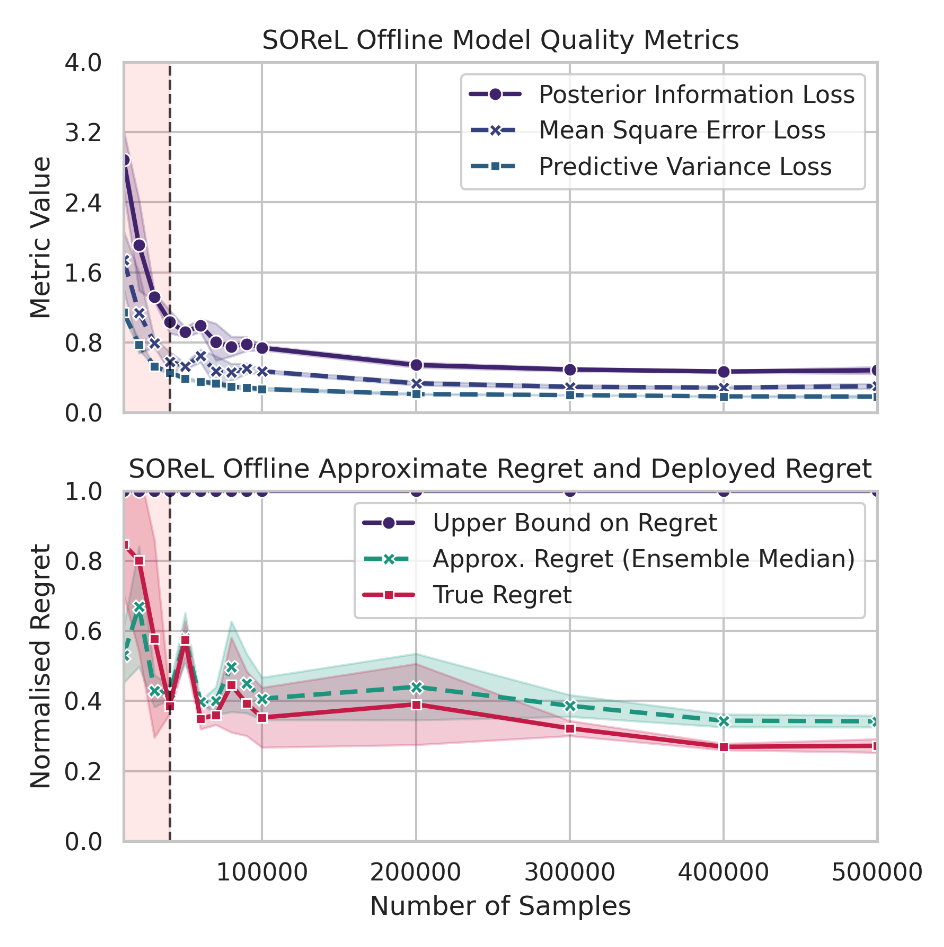
Figure 3: A simplified version of SOReL applied to brax-halfcheetah-full-replay to identify when the policy can be deployed. Shaded red indicates where $\mathcal{E}(\mathcal{D}_{N},\mathcal{M}^{\star})\not\approx\mathcal{V}(\mathcal{D}_{N})$ (for a threshold of $0.25$), and hence the approximate regret may be unreliable. Mean and standard deviation given over 3 seeds.

We demonstrate how SOReL can be implemented as a safe ORL algorithm in 5 environments: two gymnax environments and three brax environments. Referring back to Fig.˜1(b), we progressively include more offline data to learn a policy until a safe level of approximate regret is achieved. For our implementation, we use a variation of the standard Gaussian world model presented in Section˜5.3, randomised priors (Osband et al., 2018; Ciosek et al., 2020) for approximate inference and RNN-PPO (Schulman et al., 2017) to solve the BAMDP. Since we do not use a prior on the model, the offline data must be diverse, including transitions from poor, medium and expert regions of performance. While the gymnax environments we test on are simple enough that collecting a random dataset is sufficient, for the brax environments we collect our own full-replay datasets to ensure that this is the case. Implementation and dataset details are found in Appendix˜F.

In practice, each time additional offline data is incorporated, the model, approximate inference and BAMDP hyperparameters should be newly tuned. To avoid too high a computational burden in our experiments, we use fixed model and approximate inference hyperparameters, highlighting in red the region where the approximate regret may be unreliable, and only tune the BAMDP hyperparameters using the approximate regret for one seed and offline dataset size (Fig.˜7 in Section˜E.1). While we deploy each policy in the true environment to validate our approximate regret, in practice, the policy would only be deployed once the approximate regret is sufficiently low. Fig.˜3, showing results for halfcheetah-full-replay, along with all other results found in Section˜E.1, confirm that SOReL’s approximate regret is a good proxy for the true regret, allowing for the safe deployment of the Bayes-optimal policy. Using the regret and PIL, all hyperparameters can be tuned entirely offline and the practitioner can identify any issues (whether with the offline-dataset, the approximate inference method, or the model) prior to deployment. We also highlight the generalisability of our algorithm: while the policy used to collect the halfcheetah dataset achieves an expected episodic return of around 1800 (Fig.˜11 in Appendix˜E), SOReL’s policy (learned on a subset of the offline dataset) achieves a normalised regret of around 0.28 in the true environment (bottom of Fig.˜3), corresponding to an undiscounted episode return of just under 2500. As expected (Section˜6.1), our experiments show that the utility of the upper bound depends critically on the model being accurate enough relative to the discount factor. More details on a non-trivial upper-bound, along with results for gymnax and the remaining brax environments and ablations of different ensemble metrics that can be used to approximate regret with varying degrees of conservatism are found in Appendix˜E.

7.2 TOReL is an Effective Offline Hyperparameter Tuner for ORL

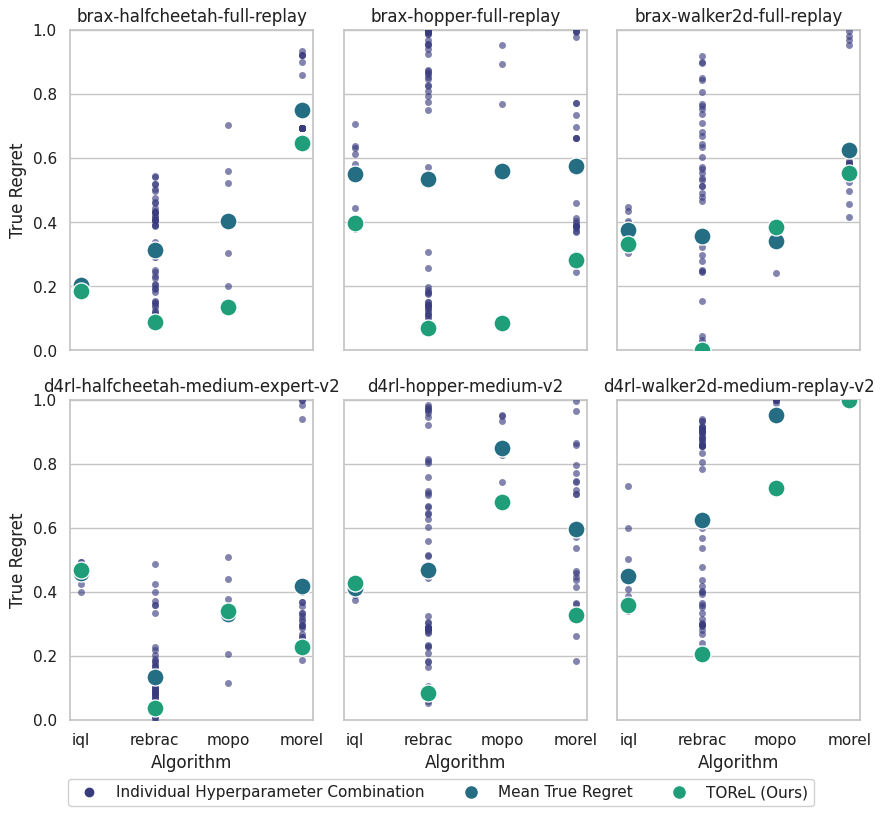
Figure 4: TOReL-selected hyperparameter regret versus mean hyperparameter regret (lower is better).

We use TOReL to identify hyperparameters for ReBRAC Tarasov et al. (2023) and IQL Kostrikov et al. (2021) (two model-free algorithms), and MOPO Yu et al. (2020) and MOReL Kidambi et al. (2020) (two model-based algorithms). Details are given in Section˜F.4. In Fig.˜4 we compare the regret of the TOReL-selected hyperparameter combination to the true regret, which we define as the expected regret over all possible hyperparameter combinations, since no algorithm provides a method of offline hyperparameter tuning. We also compare against the oracle regret: the minimum regret achieved by any hyperparameter combination. We evaluate each algorithm on 6 offline datasets: 200K randomly sampled transitions from each of our three brax datasets, and in the D4RL Fu et al. (2020) locomotion datasets suggested by  Jackson et al. (2025) (halfcheetah-medium-expert, hopper-medium and walker2d-medium-replay).

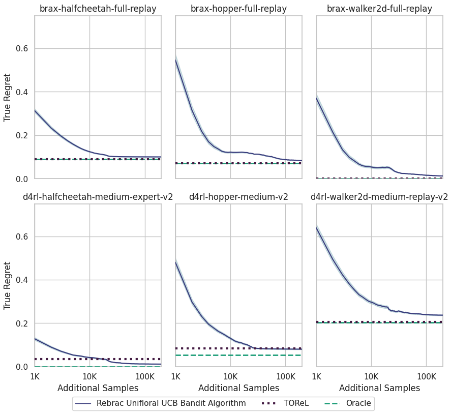
Figure 5: TOReL compared to UCB bandit-based online hyperparameter selection. The x-axis shows the additional samples required during online hyperparameter tuning. For reference, the size of the D4RL offline datasets are 1998K, 1000K and 302K (left to right). Shaded indicates the UCB 95th percentile confidence interval.

Table˜1 shows ReBRAC+TOReL as a consistently high-achieving combination, reaching near-oracle performance on every dataset. For two-thirds of the tasks and algorithms there is statistically significant ($p<0.05$), strong ($r>|0.5|$) positive ($r>0$) Pearson correlation between the ensemble median regret metric and the true regret (Table˜3 and Fig.˜10 in Appendix˜E). Where no strong positive correlation is observed (possibly due to limited hyperparameter coverage) the average TOReL regret (0.433) is still lower than the corresponding true regret (0.458). Our final experiment analyses the number of samples saved using TOReL rather than the UCB bandit-based online hyperparameter selection algorithm proposed by Jackson et al. (2025). We tune hyperparameters for ReBRAC, as ReBRAC achieves the lowest regret across all tasks and algorithms. Results for the D4RL and brax datasets are depicted in Fig.˜5. TOReL offers significant savings in terms of sample complexity compared to existing online hyperparameter tuning methods: for the D4RL datasets, 20K to >200K additional online samples are spared, while for the brax datasets >200K are spared, essentially preventing a doubling of the size of the offline dataset.

Task	Algo.	Oracle	TOReL	Oracle Mean	TOReL Mean	True
brax-halfcheetah-full-replay	ReBRAC	0.089	0.089	0.262	0.264	0.417
brax-hopper-full-replay	ReBRAC	0.070	0.070	0.193	0.209	0.554
brax-walker-full-replay	ReBRAC	0.000	0.000	0.241	0.317	0.425
d4rl-halfcheetah-medium-expert-v2	ReBRAC	0.000	0.036	0.176	0.268	0.336
d4rl-hopper-medium-v2	ReBRAC	0.053	0.083	0.380	0.323	0.580
d4rl-walker2d-medium-replay-v2	ReBRAC	0.204	0.206	0.567	0.572	0.757

Table 1: TOReL Regret Summary Statistics (lower is better): bold indicates where TOReL is within 5% of the corresponding Oracle. Left: algorithm chosen if the Oracle can choose over both hyperparameters and algorithms; corresponding oracle regret and regret of the TOReL-chosen hyperparameters for that algorithm. Middle: oracle and TOReL regrets averaged over all algorithms. Right: true regret averaged over all algorithms. For these tasks, ReBRAC+TOReL is consistently the best.

8 Conclusion

High online sample complexity and lack of performance guarantees of existing methods present a major barrier to the widespread adoption of offline RL. In this paper, we introduce SOReL and TOReL, two theoretically grounded approaches to tackle these core issues. For SOReL, we introduce a model-based Bayesian approach for offline RL and exploit predictive uncertainty to approximate regret. To tune hyperparameters and ensure accurate regret quantification, we minimise the PIL. In TOReL, we extend our fully offline hyperparameter tuning algorithm to general offline RL methods. Our empirical evaluations confirm SOReL is a reliable method for safe offline RL with accurate regret quantification and TOReL achieves near-oracle performance with offline data alone, resulting in significant savings in online samples for hyperparameter tuning without sacrificing performance.

Appendix A Broader Impact

This paper presents work whose goal is to improve the safety and efficacy of offline RL. Our work therefore takes significant steps towards the development of safe offline RL methods with accurate regret guarantees that act in ways that are predictable. We also hope our paper helps to re-frame the discourse on offline RL to focus on safety, practical efficacy and sample efficiency.

More generally, any advancement in RL should be seen in the context of general advancements to machine learning. Whilst machine learning has the potential to develop useful tools to benefit humanity, it must be carefully integrated into underlying political and social systems to avoid negative consequences for people living within them. A discussion of this complex topic lies beyond the scope of this work.

Appendix B Primer on Bayesian RL

A Bayesian epistemology characterises the agent’s uncertainty in the MDP through distributions over any unknown variable [Martin, 1967, Duff, 2002]. In our learning problem, a Bayesian first specifies a model $P_{R,S}(s_{t},a_{t})$ over the unknown state transition and reward distribution, representing a hypothesis space of possible environment dynamics. We focus on a parametric model: $p(r_{t},s_{t+1}|s_{t},a_{t},\theta)$ with each $\theta\in\Theta\subseteq\mathbb{R}^{d}$ representing a hypothesis about the MDP $\mathcal{M}^{\star}$, however our results can easily be generalised to non-parametric methods like Gaussian process regression [Rasmussen and Williams, 2006, Wiener, 1923, Krige, 1951]. A prior distribution over the parameter space $P_{\Theta}$ is specified, which represents the initial a priori belief in the true value of $P_{R,S}^{\star}(s,a)$ before the agent has observed any transitions. Priors are a powerful aspect of Bayesian RL, allowing practitioners to provide the agent with any information about the MDP and transfer knowledge between agents and domains. Given a history $h_{t}$, the prior is updated to a posterior $P_{\Theta}(h_{t})$, representing the agent’s beliefs in the MDP’s dynamics once $h_{t}$ has been observed. For each history, the posterior is used to marginalise across all hypotheses according to the agent’s uncertainty, yielding the predictive state transition-reward distribution $P_{R,S}(h_{t},a_{t})=\mathbb{E}_{\theta\sim P_{\Theta}(h_{t})}\left[P_{R,S}(s_{t},a_{t},\theta)\right]$ which characterise the epistemic and aleatoric uncertainty in $P_{R,S}^{\star}(s_{t},a_{t})$. Given $P_{R,S}(h_{t},a_{t})$, we reason over counterfactual future trajectories using the predictive distribution over trajectories $P_{t}^{\pi}$ and define the BRL objective as:

$$J^{\pi}_{\textrm{Bayes}}(P_{\Theta})\coloneqq\mathbb{E}_{h_{\infty}\sim P_{\infty}^{\pi}}\left[\sum_{i=0}^{\infty}\gamma^{i}r_{i}\right].$$ (12)

Let $\Pi_{\mathcal{H}}$ denote the space of all history-conditioned policies. A corresponding optimal policy is known as a Bayes-optimal policy, which we denote as $\pi^{\star}_{\textrm{Bayes}}(\cdot)\in\Pi^{\star}_{\textrm{Bayes}}(P_{\Theta})\coloneqq\operatorname*{arg\,max}_{\pi\in\Pi_{\mathcal{H}}}J^{\pi}_{\textrm{Bayes}}(P_{\Theta})$. Unlike in frequentist RL, Bayesian variables depend on histories obtained through posterior marginalisation; hence the posterior is often known as the belief state, which augments each ground state $s_{t}$ like in a partially observable Markov decision process [Drake, 1962, Åström, Karl Johan, 1965, Smallwood and Sondik, 1973, Kaelbling et al., 1998]. Analogously to the state-transition distribution in frequentist RL, we define a belief transition distribution $P_{\mathcal{H}}(h_{t},a_{t})$ using the predictive state transition-reward distribution, which yields Bayes-adaptive MDP (BAMDP) [Duff, 2002]: $\mathcal{M}_{\textrm{Bayes}}(P_{\Theta})\coloneqq\langle\mathcal{H},\mathcal{A},P_{0},P_{\mathcal{H}}(h,a),\gamma\rangle$. The BAMDP is solved using planning methods to obtain a Bayes-optimal policy, which naturally balances exploration with exploitation: after every timestep, the agent’s uncertainty is characterised via the posterior conditioned on the history $h_{t}$, which includes all future trajectories to marginalise over. Via the belief transition, the BRL objective accounts for how the posterior evolves on every timestep, and hence any Bayes-optimal policy $\pi^{\star}_{\textrm{Bayes}}$ is optimal not only according to the epistemic uncertainty of a fixed belief but accounts for how the epistemic uncertainty evolves at every future timestep, decaying according to the discount factor.

Appendix C Derivations

C.1 Negative Log Likelihood Loss Function with Approximate Inference

Assume a dataset of $N$ input-output pairs:

$$\mathcal{D}_{N}\coloneqq\{(x_{0},y_{0}),(x_{1},y_{1}),\dots(x_{N-1},y_{N-1})\},$$ (13)

and a multivariate Gaussian regression model:

$$p(y|x,\theta)=\frac{1}{(2\pi)^{\frac{D}{2}}}\lvert\Sigma_{\theta}(x)\rvert^{\frac{1}{2}}\exp\left(-\frac{1}{2}(y-\mu_{\theta}(x))\Sigma_{\theta}^{-1}(y-\mu_{\theta}(x))^{T}\right),$$ (14)

where $D$ is the number of dimensions. Here our model $\text{NN}_{\theta}:\mathcal{X}\rightarrow\mathcal{P(Y)}$ is a neural network parametrised by $\theta\in\Theta$ that outputs a Gaussian distribution $\mathcal{N}(\mu_{\theta},\Sigma_{\theta})$ over $\mathcal{Y}$. Assuming independent dimensions, such that the covariance matrix is diagonal:

$$p(y|x,\theta)=\prod_{d=0}^{D-1}\frac{1}{\sqrt{2\pi\sigma_{\theta_{d}}^{2}(x)}}\exp\left(-\frac{1}{2\sigma_{\theta_{d}}^{2}(x)}(y_{d}-\mu_{\theta_{d}}(x))^{2}\right).$$ (15)

We can then fit our model by minimising the negative log likelihood loss:

$$\mathcal{L}(\textrm{NLL}(\theta))$$ (16)

$$\coloneqq -\log p(\mathcal{D}_{N}|\theta),$$ (17)

$$= \sum_{i=0}^{N-1}\left(\frac{D}{2}\log(2\pi)+\frac{1}{2}\sum_{d=0}^{D-1}\left(\log\sigma_{\theta_{d}}^{2}(x_{i})+\frac{(y_{i_{d}}-\mu_{\theta_{d}}(x_{i}))^{2}}{\sigma_{\theta_{d}}^{2}(x_{i})}\right)\right),$$ (18)

$$= \left[\sum_{i=0}^{N-1}\frac{1}{N}\left(\frac{D}{2}\log(2\pi)+\frac{1}{2}\sum_{d=0}^{D-1}\left(\log\sigma_{\theta_{d}}^{2}(x_{i})+\frac{(y_{i_{d}}-\mu_{\theta_{d}}(x_{i}))^{2}}{\sigma_{\theta_{d}}^{2}(x_{i})}\right)\right)\right],$$ (19)

$$= \mathbb{E}_{i\sim\mathcal{U}_{N}}\left[\frac{D}{2}\log(2\pi)+\frac{1}{2}\sum_{d=0}^{D-1}\left(\log\sigma_{\theta_{d}}^{2}(x_{i})+\frac{(y_{i_{d}}-\mu_{\theta_{d}}(x_{i}))^{2}}{\sigma_{\theta_{d}}^{2}(x_{i})}\right)\right],$$ (20)

$$\overset{c}{=} \mathbb{E}_{i\sim\mathcal{U}_{N}}\left[\sum_{d=0}^{D-1}\left(\log\sigma_{\theta_{d}}^{2}(x_{i})+\frac{(y_{i_{d}}-\mu_{\theta_{d}}(x_{i}))^{2}}{\sigma_{\theta_{d}}^{2}(x_{i})}\right)\right],$$ (21)

where recall $\mathcal{U}_{N}$ is the uniform distribution over $\{0,1,\dots N-1\}$. Our final line means equality up to a constant, as we can ignore the $\frac{D}{2}\log(2\pi)$ term for optimisation because it is independent of $\theta$.

We use RP ensembles for our approximate posterior [Osband et al., 2018, Ciosek et al., 2020]; here an ensemble of $M$ separate model weights $\{\theta_{0},\theta_{i},\dots\theta_{M-1}\}$ are randomly initialised and are optimised in parallel, summing over the corresponding negative log likelihoods. When training, we optimise the log-variance rather than the variance for numerical stability and to ensure that the variance remains positive. This allows us to simultaneously optimise maximum and minimum log-variance parameters for each dimension across the ensemble, which we use to soft-clamp the log-variances output by individual models, preventing any individual model becoming overly confident or too uncertain in one dimension. Our final loss function is then given by:

$$\mathcal{L}(\theta,\mathcal{D}_{N}) =\sum_{j=0}^{M-1}\left(\mathbb{E}_{i\sim\mathcal{U}_{N}}\left[\sum_{d=0}^{D-1}\left(\xi_{\theta_{d_{j}}}(x_{i})+\frac{(y_{i_{d}}-\mu_{\theta_{d_{j}}}(x_{i}))^{2}}{\exp\left(\xi_{\theta_{d_{j}}}(x_{i})\right)}\right)\right]\right)$$ (22)

$$\qquad+c\cdot\sum_{d=0}^{D-1}\left(\xi_{\theta_{d_{\text{max}}}}-\xi_{\theta_{d_{\text{min}}}}\right),$$ (23)

where $\xi_{\theta_{d_{j}}}=\xi_{\theta_{d_{\text{min}}}}+\left[1+\exp\left(\xi_{\theta_{d_{\text{max}}}}-\left[1+\exp\left(\log\sigma_{\theta_{d_{j}}}^{2}-\xi_{\theta_{d_{\text{max}}}}\right)\right]-\xi_{\theta_{d_{\text{min}}}}\right)\right]$ and $\xi_{\theta_{d_{\text{min}}}}$ and $\xi_{\theta_{d_{\text{max}}}}$ are respectively the minimum and maximum log-variance parameters optimised across the ensemble, $c$ is the log-variance difference coefficient used to control the clamping term, and $M$ is the number of models in the ensemble. $\mathcal{L}(\theta,\mathcal{D}_{N})$ can be minimised by using Monte Carlo minibatch gradient descent with a minibatch $\mathcal{M}_{n}$ of $n<N$ samples drawn uniformly from $\mathcal{D}_{N}$.

C.2 Regret Approximators

Predictive Variance:

We now show how the true regret can be approximated using the Bayesian predictive variance of returns. We start with the bound on from Ineq. 48. Defining the discounted return $R(h_{\infty})\coloneqq\sum_{i=0}^{\infty}\gamma^{i}r_{i}$:

$$\left\lvert J^{\pi}(\mathcal{M}^{\star})-J^{\pi}_{\textrm{Bayes}}(P_{\Theta}(\mathcal{D}_{N}))\right\rvert =\left\lvert J^{\pi}(\mathcal{M}^{\star})-J^{\pi}_{\textrm{Bayes}}(P_{\Theta}(\mathcal{D}_{N}))\right\rvert,$$ (24)

$$=\left\lvert J^{\pi}(\mathcal{M}^{\star})-\mathbb{E}_{\theta\sim P_{\Theta}(\mathcal{D}_{N}),h_{\infty}\sim P_{\infty}^{\pi}(\theta)}\left[R(h_{\infty})\right]\right\rvert,$$ (25)

$$=\left\lvert\mathbb{E}_{\theta\sim P_{\Theta}(\mathcal{D}_{N}),h_{\infty}\sim P_{\infty}^{\pi}(\theta)}\left[J^{\pi}(\mathcal{M}^{\star})-R(h_{\infty})\right]\right\rvert,$$ (26)

$$=\sqrt{\left(\mathbb{E}_{\theta\sim P_{\Theta}(\mathcal{D}_{N}),h_{\infty}\sim P_{\infty}^{\pi}(\theta)}\left[J^{\pi}(\mathcal{M}^{\star})-R(h_{\infty})\right]\right)^{2}}.$$ (27)

Applying Jensen’s inequality:

$$\left\lvert J^{\pi}(\mathcal{M}^{\star})-J^{\pi}_{\textrm{Bayes}}(P_{\Theta}(\mathcal{D}_{N}))\right\rvert \leq\sqrt{\mathbb{E}_{\theta\sim P_{\Theta}(\mathcal{D}_{N}),h_{\infty}\sim P_{\infty}^{\pi}(\theta)}\left[\left(J^{\pi}(\mathcal{M}^{\star})-R(h_{\infty})\right)^{2}\right]}.$$ (28)

We now recognise that the mean squared error term in Eq.˜28 relies on knowing the true MDP dynamics $J^{\pi}(\mathcal{M}^{\star})$. We can approximate this term using the using the predictive variance over returns:

$$\mathbb{E}_{\theta\sim P_{\Theta}(\mathcal{D}_{N}),h_{\infty}\sim P_{\infty}^{\pi}(\theta)}\left[\left(J^{\pi}(\mathcal{M}^{\star})-R(h_{\infty})\right)^{2}\right]$$ (29)

$$\qquad\approx\mathbb{E}_{\theta\sim P_{\Theta}(\mathcal{D}_{N}),h_{\infty}\sim P_{\infty}^{\pi}(\theta)}\left[\left(J^{\pi}_{\textrm{Bayes}}(\mathcal{D}_{N})-R(h_{\infty})\right)^{2}\right],$$ (30)

$$\qquad=\mathbb{V}_{\theta\sim P_{\Theta}(\mathcal{D}_{N}),h_{\infty}\sim P_{\infty}^{\pi}(\theta)}\left[R(h_{\infty})\right],$$ (31)

which can be estimated using the dataset $\mathcal{D}_{N}$, yielding:

$$\left\lvert J^{\pi}(\mathcal{M}^{\star})-J^{\pi}_{\textrm{Bayes}}(P_{\Theta}(\mathcal{D}_{N}))\right\rvert\leq\sqrt{\mathbb{V}_{\theta\sim P_{\Theta}(\mathcal{D}_{N}),h_{\infty}\sim P_{\infty}^{\pi}(\theta)}\left[R(h_{\infty})\right]}.$$ (32)

Finally, using Ineq. 48 this justifies our approximation for estimating the regret:

$$\textnormal{{Regret}}(\mathcal{M}^{\star},\mathcal{D}_{N})\approx 2\sqrt{\mathbb{V}_{\theta\sim P_{\Theta}(\mathcal{D}_{N}),h_{\infty}\sim P_{\infty}^{\pi}(\theta)}\left[R(h_{\infty})\right]}.$$ (33)

To improve the approximation, we conservatively upper-bound the regret based on alternate ensemble statistics with varying degrees of conservatism to prevent associating a low regret with a policy that performs equally poorly in all members of the ensemble:

$$\textnormal{{Regret}}(\mathcal{M}^{\star},\mathcal{D}_{N})\approx\max\Big{[} 2\sqrt{\mathbb{V}_{\theta\sim P_{\Theta}(\mathcal{D}_{N}),h_{\infty}\sim P_{\infty}^{\pi}(\theta)}\left[R(h_{\infty})\right]},$$

$$\hat{R}_{\max}-\hat{\mathbb{M}}_{\theta\sim P_{\Theta}(\mathcal{D}_{N}),h_{\infty}\sim P_{\infty}^{\pi}(\theta)}\left[R(h_{\infty})\right]\Big{]},$$ (34)

for example, here $\hat{\mathbb{M}}_{\theta\sim P_{\Theta}(\mathcal{D}_{N}),h_{\infty}\sim P_{\infty}^{\pi}(\theta)}\left[R(h_{\infty})\right]$ denotes the median predictive returns based on sampling from the (approximate) posterior and rolling out the Bayes-optimal policy. $\hat{R}_{\max}$ is estimated from the maximum return in the offline dataset. In Fig.˜7 and Fig.˜9, we plot different ensemble statistics (the ensemble mean, median, maximum and minimum regrets) that can be used to inform the approximate regret: we shade the regret based on the range of these statistics in purple. As long as the true environment falls in the space spanned by the posterior (model ensemble), the true regret is guaranteed to lie within this range. By ensuring that the (normalised) predictive variance is at least as large as the (normalised) MSE in the PIL, the space spanned by the approximate posterior via model ensemble is approximately large enough, relative to the model error. Below we order different ensemble statistics from least to most conservative:

$$\textnormal{{Regret}}(\mathcal{M}^{\star},\mathcal{D}_{N})\approx \hat{R}_{\max}-\hat{R}_{\theta\sim P_{\Theta}(\mathcal{D}_{N}),h_{\infty}\sim P_{\infty}^{\pi}(\theta)}\left[R(h_{\infty})\right],$$ (35)

$$\leq \hat{R}_{\max}-\hat{\mathbb{E}}_{\theta\sim P_{\Theta}(\mathcal{D}_{N}),h_{\infty}\sim P_{\infty}^{\pi}(\theta)}\left[R(h_{\infty})\right],$$ (36)

$$\approx \hat{R}_{\max}-\hat{\mathbb{M}}_{\theta\sim P_{\Theta}(\mathcal{D}_{N}),h_{\infty}\sim P_{\infty}^{\pi}(\theta)}\left[R(h_{\infty})\right],$$ (37)

$$\leq \hat{R}_{\max}-\hat{r}_{\theta\sim P_{\Theta}(\mathcal{D}_{N}),h_{\infty}\sim P_{\infty}^{\pi}(\theta)}\left[R(h_{\infty})\right].$$ (38)

Here $\hat{R}_{\theta\sim P_{\Theta}(\mathcal{D}_{N}),h_{\infty}\sim P_{\infty}^{\pi}(\theta)}\left[R(h_{\infty})\right]$, $\hat{\mathbb{E}}_{\theta\sim P_{\Theta}(\mathcal{D}_{N}),h_{\infty}\sim P_{\infty}^{\pi}(\theta)}\left[R(h_{\infty})\right]$, and $\hat{r}_{\theta\sim P_{\Theta}(\mathcal{D}_{N}),h_{\infty}\sim P_{\infty}^{\pi}(\theta)}\left[R(h_{\infty})\right]$, respectively denote the maximum, mean, and minimum predictive returns based on sampling from the (approximate) posterior and rolling out the Bayes-optimal policy. We note that the minimum predictive return leads to the maximum predictive regret: "Ensemble Max" in Fig.˜7 and Fig.˜9 refer to the maximum predictive regrets rather than maximum predictive returns. Empirically, we find that the ensemble median alone is a good proxy for the true regret, being neither overly conservative, nor overly susceptible to being skewed by a policy that performs well on only a subset of posterior samples (as the mean might be). Using the variance, a policy with high variance but also high mean will be associated with a high approximate regret, which is the case for brax-hopper-full-replay (Fig.˜9(c)), where the variance actually overestimates the regret.

Appendix D Proofs

D.1 Primer on Total Variational Distance

We measure distance between two probability distributions $P_{X}$ and $Q_{X}$ using the total variational (TV) distance, defined as:

$$\textrm{TV}(P_{X}\|Q_{X}) \coloneqq\sup_{E}\left\lvert P_{X}(E)-Q_{X}(E)\right\rvert.$$ (39)

The TV distance takes the supremum over all events $E$ to find the event that gives rise to the maximum difference in probability between two distributions. A key property of the TV distance is: $0\leq\textrm{TV}(P_{X}\|Q_{X})\leq 1$. If $\textrm{TV}(P_{X}\|Q_{X})=0$, then $P_{X}=Q_{X}$ as there is no event that both distributions don’t assign the same probability mass to. If $\textrm{TV}(P_{X}\|Q_{X})=1$, then the distributions assign completely different mass to at least one event. The TV distance can be related to the Kullback-Leibler (KL) divergence using the Bretagnolle-Huber [Bretagnolle and Huber, 1978] inequality: $\textrm{TV}(P_{X}\|Q_{X})\leq\sqrt{1-\exp\left(-\textrm{KL}(P_{X}\|Q_{X})\right)}\leq 1$, which preserves the property that $0\leq\textrm{TV}(P_{X}\|Q_{X})\leq 1$. The TV distance can be shown [Sriperumbudur et al., 2009] to be equivalent to the integral probability metric under the $\infty$-norm, which we will make use of in our theorems:

$$\textrm{TV}(P_{X}\|Q_{X}) =\frac{1}{2}\sup_{f\in\mathcal{F}:\mathcal{X}\rightarrow[-1,1]}\left\lvert\mathbb{E}_{x\sim P_{X}}\left[f(x)\right]-\mathbb{E}_{x\sim Q_{X}}\left[f(x)\right]\right\rvert,$$ (40)

In this form, the supremum is taken over the space of all functions that are bounded by unity, that is $\lVert f\rVert_{\infty}=1$.

D.2 Proof of Theorem˜1

Let the predictive distribution over history $h_{t}$ using the posterior $P_{\Theta}(\mathcal{D}_{N})$ be $P_{t,\pi}(\mathcal{D}_{N})$, which has density:

$$p_{\pi}(h_{t},\mathcal{D}_{N})\coloneqq p_{0}(s_{0})\prod_{i=0}^{t-1}\pi(a_{i}|h_{i})p(r_{i}|h_{i},a_{i},\mathcal{D}_{N})p(s_{i+1}|h_{i},a_{i},\mathcal{D}_{N}).$$ (41)

To make progress towards quantifying how much offline data we need to achieve an acceptable level of regret, we first relate the true regret $\textnormal{{Regret}}(\mathcal{M}^{\star},\mathcal{D}_{N})$ to the TV distance between the true $P_{i,\pi}^{\star}$ and predictive $P_{i,\pi}(\mathcal{D}_{N})$ history distributions:

Lemma 1.

Let $\mathcal{R}_{\max}\coloneqq\frac{(r_{\textrm{max}}-r_{\textrm{min}})}{1-\gamma}$ denote the maximum possible regret for the MDP. For a prior $P_{\Theta}(\mathcal{D}_{N})$, the true regret can be bounded as:

$$\textnormal{{Regret}}(\mathcal{M}^{\star},\mathcal{D}_{N}) \leq 2\mathcal{R}_{\max}\cdot\sup_{\pi}\mathbb{E}_{i\sim\mathcal{G}(\gamma)}\left[\textrm{TV}\left(P_{i+1,\pi}^{\star}\|P_{i+1}^{\pi}(\mathcal{D}_{N})\right)\right].$$ (42)

Proof.

We start from the definition of the true regret:

$$\textnormal{{Regret}}(\mathcal{M}^{\star},\mathcal{D}_{N})\coloneqq J^{\pi^{\star}}(\mathcal{M}^{\star})-J^{\pi_{\textrm{Bayes}}^{\star}}(\mathcal{M}^{\star},\mathcal{D}_{N}).$$ (43)

We now bound the difference between $J^{\pi^{\star}}(\mathcal{M}^{\star})$ and $J^{\pi_{\textrm{Bayes}}^{\star}}(\mathcal{M}^{\star},\mathcal{D}_{N})$ in terms of the difference between $J^{\pi}(\mathcal{M}^{\star})$ and $J^{\pi}_{\textrm{Bayes}}(\mathcal{D}_{N})$:

$$\textnormal{{Regret}}(\mathcal{M}^{\star},\mathcal{D}_{N})$$ (44)

$$=J^{\pi^{\star}}(\mathcal{M}^{\star})-J^{\pi^{\star}}_{\textrm{Bayes}}(P_{\Phi}(\mathcal{D}_{N}))+J^{\pi^{\star}}_{\textrm{Bayes}}(P_{\Phi}(\mathcal{D}_{N}))-J^{\pi_{\textrm{Bayes}}^{\star}}(\mathcal{M}^{\star},\mathcal{D}_{N}),$$ (45)

$$\leq J^{\pi^{\star}}(\mathcal{M}^{\star})-J^{\pi^{\star}}_{\textrm{Bayes}}(P_{\Phi}(\mathcal{D}_{N}))+J^{\pi^{\star}_{\textrm{Bayes}}}_{\textrm{Bayes}}(P_{\Phi}(\mathcal{D}_{N}))-J^{\pi_{\textrm{Bayes}}^{\star}}(\mathcal{M}^{\star},\mathcal{D}_{N}),$$ (46)

$$\leq\sup_{\pi}\left\lvert J^{\pi}(\mathcal{M}^{\star})-J^{\pi}_{\textrm{Bayes}}(P_{\Theta}(\mathcal{D}_{N}))\right\rvert+\sup_{\pi}\left\lvert J^{\pi}_{\textrm{Bayes}}(P_{\Theta}(\mathcal{D}_{N}))-J^{\pi}(\mathcal{M}^{\star})\right\rvert,$$ (47)

$$=2\sup_{\pi}\left\lvert J^{\pi}(\mathcal{M}^{\star})-J^{\pi}_{\textrm{Bayes}}(P_{\Theta}(\mathcal{D}_{N}))\right\rvert,$$ (48)

where the second line follows from $J^{\pi^{\star}}_{\textrm{Bayes}}(P_{\Phi}(\mathcal{D}_{N}))\leq J^{\pi^{\star}_{\textrm{Bayes}}}_{\textrm{Bayes}}(P_{\Phi}(\mathcal{D}_{N}))$ by definition. Now our goal is to bound $\left\lvert J^{\pi}(\mathcal{M}^{\star})-J^{\pi}_{\textrm{Bayes}}(P_{\Theta}(\mathcal{D}_{N}))\right\rvert$:

$$\left\lvert J^{\pi}(\mathcal{M}^{\star})-J^{\pi}_{\textrm{Bayes}}(P_{\Theta}(\mathcal{D}_{N}))\right\rvert =\left\lvert\mathbb{E}_{h_{\infty}\sim P^{\star}_{\infty,\pi}}\left[\sum_{i=0}^{\infty}\gamma^{i}r_{i}\right]-\mathbb{E}_{h_{\infty}\sim P^{\pi}_{\infty}(\mathcal{D}_{N})}\left[\sum_{i=0}^{\infty}\gamma^{i}r_{i}\right]\right\rvert,$$ (49)

$$=\left\lvert\sum_{i=0}^{\infty}\gamma^{i}\mathbb{E}_{h_{i+1}\sim P^{\star}_{i+1,\pi}}\left[r_{i}\right]-\sum_{i=0}^{\infty}\gamma^{i}\mathbb{E}_{h_{i+1}\sim P^{\pi}_{i+1}(\mathcal{D}_{N})}\left[r_{i}\right]\right\rvert,$$ (50)

$$=\left\lvert\sum_{i=0}^{\infty}\gamma^{i}\left(\mathbb{E}_{h_{i+1}\sim P^{\star}_{i+1,\pi}}\left[r_{i}\right]-\mathbb{E}_{h_{i+1}\sim P^{\pi}_{i+1}(\mathcal{D}_{N})}\left[r_{i}\right]\right)\right\rvert,$$ (51)

$$\leq\sum_{i=0}^{\infty}\gamma^{i}\left\lvert\mathbb{E}_{h_{i+1}\sim P^{\star}_{i+1,\pi}}\left[r_{i}\right]-\mathbb{E}_{h_{i+1}\sim P^{\pi}_{i+1}(\mathcal{D}_{N})}\left[r_{i}\right]\right\rvert.$$ (52)

Using Ineq. 59 from Lemma˜2, we now bound each difference $\left\lvert\mathbb{E}_{h_{i+1}\sim P^{\star}_{i+1,\pi}}\left[r_{i}\right]-\mathbb{E}_{h_{i+1}\sim P^{\pi}_{i+1}(\mathcal{D}_{N})}\left[r_{i}\right]\right\rvert$ in terms of total variational distance between $P^{\star}_{i+1,\pi}$ and $P^{\pi}_{i+1}(\mathcal{D}_{N})$:

$$\left\lvert J^{\pi}(\mathcal{M}^{\star})-J^{\pi}_{\textrm{Bayes}}(P_{\Theta}(\mathcal{D}_{N}))\right\rvert \leq(r_{\max}-r_{\min})\cdot\sum_{i=0}^{\infty}\gamma^{i}\textnormal{{TV}}\left(P^{\star}_{i+1,\pi}\|P^{\pi}_{i+1}(\mathcal{D}_{N})\right),$$ (53)

$$=\frac{r_{\max}-r_{\min}}{1-\gamma}\cdot\sum_{i=0}^{\infty}(1-\gamma)\gamma^{i}\textnormal{{TV}}\left(P^{\star}_{i+1,\pi}\|P^{\pi}_{i+1}(\mathcal{D}_{N})\right),$$ (54)

$$=\frac{r_{\max}-r_{\min}}{1-\gamma}\cdot\mathbb{E}_{i\sim\mathcal{G}(\gamma)}\left[\textnormal{{TV}}\left(P^{\star}_{i+1,\pi}\|P^{\pi}_{i+1}(\mathcal{D}_{N})\right)\right],$$ (55)

$$=\mathcal{R}_{\max}\cdot\mathbb{E}_{i\sim\mathcal{G}(\gamma)}\left[\textnormal{{TV}}\left(P^{\star}_{i+1,\pi}\|P^{\pi}_{i+1}(\mathcal{D}_{N})\right)\right],$$ (56)

where $\mathcal{G}(\gamma)$ is the geometric distribution. Finally, substituting into Ineq. 48 yields our desired result:

$$\textnormal{{Regret}}(\mathcal{M}^{\star},\mathcal{D}_{N}) \leq 2\sup_{\pi}\left\lvert(\mathcal{R}_{\max}\cdot\mathbb{E}_{i\sim\mathcal{G}(\gamma)}\left[\textrm{TV}\left(P^{\star}_{i+1,\pi}\|P^{\pi}_{i+1}(\mathcal{D}_{N}))\right)\right]\right\rvert,$$ (57)

$$=2\mathcal{R}_{\max}\cdot\sup_{\pi}\mathbb{E}_{i\sim\mathcal{G}(\gamma)}\left[\textrm{TV}\left(P^{\star}_{i+1,\pi}\|P^{\pi}_{i+1}(\mathcal{D}_{N}))\right)\right].$$ (58)

∎

We remark that Lemma˜1 holds for any general reward-transition model given bounded rewards. The bound in Ineq. 42 proves the true regret is governed by the geometric average of TV distances: $\mathbb{E}_{i\sim\mathcal{G}(\gamma)}\left[\textnormal{TV}\left(P^{\star}_{i+1,\pi}\|P^{\pi}_{i+1}(\mathcal{D}_{N}))\right)\right]$. As each term $\textnormal{TV}\left(P^{\star}_{i+1,\pi}\|P^{\pi}_{i+1}(\mathcal{D}_{N}))\right)$ measures the distance between the true and predictive distributions over history $h_{i}$ of length $i$, the discounting factor $\gamma$ determines how much long term histories contribute to regret.

Intuitively, the more mass the posterior places close to the true value $\theta^{\star}\in\Theta^{\star}$, the smaller each TV distance becomes, with regret tending to zero for $P_{i+1,\pi}(\mathcal{D}_{N})\approx P_{i+1,\pi}^{\star}\implies\textnormal{TV}\left(P^{\star}_{i+1,\pi}\|P^{\pi}_{i+1}(\mathcal{D}_{N}))\right)\approx 0$. Conversely, a strong but highly incorrect prior will concentrate mass around MDPs whose dynamics oppose the true dynamics, yielding $\textnormal{TV}\left(P^{\star}_{i+1,\pi}\|P^{\pi}_{i+1}(\mathcal{D}_{N}))\right)\approx 1$ for all $i$, achieving the highest possible regret: $\mathcal{R}_{\max}\coloneqq\nicefrac{{(r_{\textrm{max}}-r_{\textrm{min}})}}{{1-\gamma}}$. The resulting Bayes-optimal policy would choose actions that encourage negative reward-seeking behaviour, being farthest from optimal in terms of expected returns.

Our next lemma

Lemma 2.

For bounded reward functions:

$$\left\lvert\mathbb{E}_{h_{i+1}\sim P^{\star}_{i+1,\pi}}\left[r_{i}\right]-\mathbb{E}_{h_{i+1}\sim P^{\pi}_{i+1}(\mathcal{D}_{N})}\left[r_{i}\right]\right\rvert\leq(r_{\max}-r_{\min})\cdot\textnormal{{TV}}\left(P^{\star}_{i+1,\pi}\|P^{\pi}_{i+1}(\mathcal{D}_{N})\right).$$ (59)

Proof.

We start by subtracting and adding $\frac{r_{\max}+r_{\min}}{2}$ to the left hand side of Ineq. 59:

$$\lvert\mathbb{E}_{h_{i+1}\sim P^{\star}_{i+1,\pi}}\left[r_{i}\right]-\mathbb{E}_{h_{i+1}\sim P^{\pi}_{i+1}(\mathcal{D}_{N})}\left[r_{i}\right]\rvert$$ (60)

$$=\left\lvert\mathbb{E}_{h_{i+1}\sim P^{\star}_{i+1,\pi}}\left[r_{i}-\frac{r_{\max}+r_{\min}}{2}\right]-\mathbb{E}_{h_{i+1}\sim P^{\pi}_{i+1}(\mathcal{D}_{N})}\left[r_{i}-\frac{r_{\max}+r_{\min}}{2}\right]\right\rvert,$$ (61)

$$=\left\lvert\mathbb{E}_{h_{i+1}\sim P^{\star}_{i+1,\pi}}\left[\frac{2r_{i}-(r_{\max}+r_{\min})}{2}\right]-\mathbb{E}_{h_{i+1}\sim P^{\pi}_{i+1}(\mathcal{D}_{N})}\left[\frac{2r_{i}-(r_{\max}+r_{\min})}{2}\right]\right\rvert,$$ (62)

$$=\frac{(r_{\max}-r_{\min})}{2}\cdot\left\lvert\mathbb{E}_{h_{i+1}\sim P^{\star}_{i+1,\pi}}\left[\frac{2r_{i}-(r_{\max}+r_{\min})}{r_{\max}-r_{\min}}\right]-\mathbb{E}_{h_{i+1}\sim P^{\pi}_{i+1}(\mathcal{D}_{N})}\left[\frac{2r_{i}-(r_{\max}+r_{\min})}{r_{\max}-r_{\min}}\right]\right\rvert,$$ (63)

$$=\frac{(r_{\max}-r_{\min})}{2}\cdot\left\lvert\mathbb{E}_{h_{i+1}\sim P^{\star}_{i+1,\pi}}\left[r_{\textrm{norm}}(h_{i+1})\right]-\mathbb{E}_{h_{i+1}\sim P^{\pi}_{i+1}(\mathcal{D}_{N})}\left[r_{\textrm{norm}}(h_{i+1})\right]\right\rvert,$$ (64)

where:

$$r_{\textrm{norm}}(h_{i+1})\coloneqq\frac{2r_{i}-(r_{\max}+r_{\min})}{r_{\max}-r_{\min}}.$$ (65)

Now, as $r_{\textrm{norm}}:\mathcal{H}_{i+1}\rightarrow[-1,1]$, we can bound Eq.˜64 using the integral probability metric form of the TV distance (see Eq.˜40), yielding our desired result:

$$\lvert\mathbb{E}_{h_{i+1}\sim P^{\star}_{i+1,\pi}}\left[r_{i}\right]-\mathbb{E}_{h_{i+1}\sim P^{\pi}_{i+1}(\mathcal{D}_{N})}\left[r_{i}\right]\rvert$$ (66)

$$\leq\frac{r_{\max}-r_{\min}}{2}\cdot\sup_{f\in\mathcal{F}:\mathcal{H}_{i+1}\rightarrow[-1,1]}\left\lvert\mathbb{E}_{h_{i+1}\sim P^{\star}_{i+1,\pi}}\left[f(h_{i+1})\right]-\mathbb{E}_{h_{i+1}\sim P^{\pi}_{i+1}(\mathcal{D}_{N})}\left[f(h_{i+1})\right]\right\rvert,$$ (67)

$$=(r_{\max}-r_{\min})\cdot\textnormal{{TV}}\left(P^{\star}_{i+1,\pi}\|P^{\pi}_{i+1}(\mathcal{D}_{N})\right).$$ (68)

∎

We proved in Lemma˜1 that the rate of convergence of the sum of discounted TV distances between the true and predictive history distributions governs the rate of decrease in regret decreases with increasing data. Using the Bretagnolle-Huber inequality (see Section˜D.1), we now relate the sum of discounted TV distances to a sum of KL divergences, allowing us to control the expected regret using the PIL.

Theorem 1.

Using the PIL in Eq.˜4,the true regret is bounded as:

$$\textnormal{{Regret}}(\mathcal{M}^{\star},\mathcal{D}_{N})\leq 2\mathcal{R}_{\max}\cdot\sup_{\pi}\sqrt{1-\exp\left(-\frac{\mathcal{I}_{N}^{\pi}}{1-\gamma}\right)}$$ (69)

Proof.

Starting with the bounded derived in Ineq. 42 of Lemma˜1, we apply the Bretagnolle-Huber inequality [Bretagnolle and Huber, 1978] (see Section˜D.1) to bound the TV distance terms using the KL divergence:

$$\textnormal{{Regret}}(\mathcal{M}^{\star},\mathcal{D}_{N}) \leq 2\mathcal{R}_{\max}\cdot\sup_{\pi}\mathbb{E}_{i\sim\mathcal{G}(\gamma)}\left[\textrm{TV}\left(P^{\star}_{i+1,\pi}\|P^{\pi}_{i+1}(\mathcal{D}_{N}))\right)\right],$$ (70)

$$\leq 2\mathcal{R}_{\max}\cdot\sup_{\pi}\mathbb{E}_{i\sim\mathcal{G}(\gamma)}\left[\sqrt{1-\exp\left(-\textrm{KL}\left(P^{\star}_{i+1,\pi}\|P^{\pi}_{i+1}(\mathcal{D}_{N}))\right)\right)}\right].$$ (71)

We make two observations. Firstly, as the KL divergence is convex in its second argument and $P_{i+1,\pi}(\mathcal{D}_{N})=\mathbb{E}_{\theta\sim P_{\Theta}(\mathcal{D}_{N})}\left[P_{i+1}^{\pi}(\theta)\right]$, we can bound each KL divergence term using Jensen’s inequality as:

$$\textrm{KL}\left(P^{\star}_{i+1,\pi}\|P^{\pi}_{i+1}(\mathcal{D}_{N}))\right)\leq\mathbb{E}_{\theta\sim P_{\Theta}(\mathcal{D}_{N})}\left[\textrm{KL}\left(P_{i+1,\pi}^{\star}\|P_{i+1}^{\pi}(\theta)\right)\right].$$ (72)

Secondly, as the function $f(x)=\sqrt{1-\exp(-x)}$ is monotonically increasing in $x$, it follows that $f(x)\leq f(x^{\prime})$ for any $x\leq x^{\prime}$, hence:

$$\sqrt{1-\exp\left(-\textrm{KL}\left(P^{\star}_{i+1,\pi}\|P^{\pi}_{i+1}(\mathcal{D}_{N}))\right)\right)}\leq\sqrt{1-\exp\left(-\mathbb{E}_{\theta\sim P_{\Theta}(\mathcal{D}_{N})}\left[\textrm{KL}\left(P_{i+1,\pi}^{\star}\|P_{i+1}^{\pi}(\theta)\right)\right]\right)}$$ (73)

Applying this bound to Ineq. 71 yields:

$$\mathbb{E}_{i\sim\mathcal{G}(\gamma)} \left[\sqrt{1-\exp\left(-\textrm{KL}\left(P^{\star}_{i+1,\pi}\|P^{\pi}_{i+1}(\mathcal{D}_{N}))\right)\right)}\right]$$ (74)

$$\leq\mathbb{E}_{i\sim\mathcal{G}(\gamma)}\left[\sqrt{1-\exp\left(-\mathbb{E}_{\theta\sim P_{\Theta}(\mathcal{D}_{N})}\left[\textrm{KL}\left(P_{i+1,\pi}^{\star}\|P_{i+1}^{\pi}(\theta)\right)\right]\right)}\right].$$ (75)

As the function $f(x)=\sqrt{1-\exp(-x)}$ is concave in $x$, we can apply Jensen’s inequality, yielding:

$$\mathbb{E}_{i\sim\mathcal{G}(\gamma)} \left[\sqrt{1-\exp\left(-\textrm{KL}\left(P^{\star}_{i+1,\pi}\|P^{\pi}_{i+1}(\mathcal{D}_{N}))\right)\right)}\right]$$ (76)

$$\leq\sqrt{1-\exp\left(-\mathbb{E}_{i\sim\mathcal{G}(\gamma)}\left[\mathbb{E}_{\theta\sim P_{\Theta}(\mathcal{D}_{N})}\left[\textrm{KL}\left(P_{i+1,\pi}^{\star}\|P_{i+1}^{\pi}(\theta)\right)\right]\right]\right)}.$$ (77)

Examining the KL divergence term:

KL $$\left(P^{\star}_{i+1,\pi}\|P^{\pi}_{i+1}(\theta)\right)$$ (78)

$$=\mathbb{E}_{h_{i+1}\sim P_{i+1,\pi}^{\star}}\left[\log\left(\frac{d_{0}(s_{0})\prod_{j=0}^{i}\pi(a_{j}|h_{j})p^{\star}(r_{j}|s_{j},a_{j})p^{\star}(s_{j+1}|s_{j},a_{j})}{d_{0}(s_{0})\prod_{j=0}^{i}\pi(a_{j}|h_{j})p(r_{j}|s_{j},a_{j},\theta)p(s_{j+1}|s_{j},a_{j},\theta)}\right)\right],$$ (79)

$$=\mathbb{E}_{h_{i+1}\sim P_{i+1,\pi}^{\star}}\left[\log\left(\frac{\prod_{j=0}^{i}p^{\star}(r_{j}|s_{j},a_{j})p^{\star}(s_{j+1}|s_{j},a_{j})}{\prod_{j=0}^{i}p(r_{j}|s_{j},a_{j},\theta)p(s_{j+1}|s_{j},a_{j},\theta)}\right)\right],$$ (80)

$$=\mathbb{E}_{h_{i+1}\sim P_{i+1,\pi}^{\star}}\Bigg{[}\sum_{j=0}^{i}\Big{(}\log p^{\star}(r_{j}|s_{j},a_{j})-\log p(r_{j}|s_{j},a_{j},\theta)$$ (81)

$$\qquad\qquad\qquad\quad+\log p^{\star}(s_{j+1}|s_{j},a_{j})-\log p(s_{j+1}|s_{j},a_{j},\theta)\Big{)}\Bigg{]},$$ (82)

$$=\sum_{j=0}^{i}\mathbb{E}_{h_{j}\sim P_{j,\pi}^{\star}}\Bigg{[}\Big{(}\log p^{\star}(r_{j}|s_{j},a_{j})-\log p(r_{j}|s_{j},a_{j},\theta)$$ (83)

$$\qquad\qquad\qquad\quad+\log p^{\star}(s_{j+1}|s_{j},a_{j})-\log p(s_{j+1}|s_{j},a_{j},\theta)\Big{)}\Bigg{]},$$ (84)

$$=\sum_{j=0}^{i}\mathbb{E}_{s_{j},a_{j}\sim P^{\star}_{j,\pi}}\Bigg{[}\mathbb{E}_{r_{j},s_{j+1}\sim P_{R,S}^{\star}(s_{j},a_{j})}\Bigg{[}\Big{(}\log p^{\star}(r_{j}|s_{j},a_{j})-\log p(r_{j}|s_{j},a_{j},\theta)$$ (85)

$$\qquad\qquad\qquad\quad+\log p^{\star}(s_{j+1}|s_{j},a_{j})-\log p(s_{j+1}|s_{j},a_{j},\theta)\Big{)}\Bigg{]}\Bigg{]},$$ (86)

$$=\sum_{j=0}^{i}\mathbb{E}_{s_{j},a_{j}\sim P^{\star}_{j,\pi}}\Bigg{[}\mathbb{E}_{r_{j},s_{j+1}\sim P_{R,S}^{\star}(s_{j},a_{j})}\Bigg{[}\Big{(}\log p^{\star}(r_{j},s_{j+1}|s_{j},a_{j})$$ (87)

$$\qquad\qquad\qquad\quad-\log p(r_{j},s_{j+1}|s_{j},a_{j},\theta)\Bigg{]}\Bigg{]},$$ (88)

$$=\sum_{j=0}^{i}\mathbb{E}_{s,a\sim P^{\star}_{j,\pi}}\left[\textrm{KL}(P_{R,S}^{\star}(s,a)\|P_{R,S}(s,a,\theta))\right],$$ (89)

hence:

$$\mathbb{E}_{i\sim\mathcal{G}(\gamma)}\left[\mathbb{E}_{\theta\sim P_{\Theta}(\mathcal{D}_{N})}\left[\textrm{KL}\left(P_{i+1,\pi}^{\star}\|P_{i+1}^{\pi}(\theta)\right)\right]\right]$$ (90)

$$=\mathbb{E}_{\theta\sim P_{\Theta}(\mathcal{D}_{N})}\left[\mathbb{E}_{i\sim\mathcal{G}(\gamma)}\left[\sum_{j=0}^{i}\mathbb{E}_{s,a\sim P^{\star}_{j,\pi}}\left[\textrm{KL}(P_{R,S}^{\star}(s,a)\|P_{R,S}(s,a,\theta))\right]\right]\right],$$ (91)

$$=\mathbb{E}_{\theta\sim P_{\Theta}(\mathcal{D}_{N})}\left[\sum_{i=0}^{\infty}(1-\gamma)\gamma^{i}\sum_{j=0}^{i}\mathbb{E}_{s,a\sim P^{\star}_{j,\pi}}\left[\textrm{KL}(P_{R,S}^{\star}(s,a)\|P_{R,S}(s,a,\theta))\right]\right],$$ (92)

$$=\mathbb{E}_{\theta\sim P_{\Theta}(\mathcal{D}_{N})}\left[\sum_{i=0}^{\infty}(1-\gamma)\gamma^{i}(i+1)\sum_{j=0}^{i}\frac{1}{i+1}\mathbb{E}_{s,a\sim P^{\star}_{j,\pi}}\left[\textrm{KL}(P_{R,S}^{\star}(s,a)\|P_{R,S}(s,a,\theta))\right]\right],$$ (93)

$$=\frac{1}{1-\gamma}\mathbb{E}_{\theta\sim P_{\Theta}(\mathcal{D}_{N})}\left[\sum_{i=0}^{\infty}(1-\gamma)^{2}\gamma^{i}(i+1)\mathbb{E}_{j\sim\mathcal{U}_{i}}\left[\mathbb{E}_{s,a\sim P^{\star}_{j,\pi}}\left[\textrm{KL}(P_{R,S}^{\star}(s,a)\|P_{R,S}(s,a,\theta))\right]\right]\right],$$ (94)

$$=\frac{1}{1-\gamma}\mathbb{E}_{\theta\sim P_{\Theta}(\mathcal{D}_{N})}\left[\mathbb{E}_{i\sim\mathcal{AG(\gamma)}}\left[\mathbb{E}_{j\sim\mathcal{U}_{i}}\left[\mathbb{E}_{s,a\sim P^{\star}_{j,\pi}}\left[\textrm{KL}(P_{R,S}^{\star}(s,a)\|P_{R,S}(s,a,\theta))\right]\right]\right]\right].$$ (95)

Now, as $\rho_{\pi}^{\star}=\mathbb{E}_{i\sim\mathcal{AG(\gamma)}}\left[\mathbb{E}_{j\sim\mathcal{U}_{i}}\left[P_{j,\pi}^{\star}\right]\right]$ is the arithemetico-geometric ergodic state-action distribution, we can simplify Eq.˜95 to yield:

$$\mathbb{E}_{i\sim\mathcal{G}(\gamma)}\left[\mathbb{E}_{\theta\sim P_{\Theta}(\mathcal{D}_{N})}\left[\textrm{KL}\left(P_{i+1,\pi}^{\star}\|P_{i+1}^{\pi}(\theta)\right)\right]\right]$$ (96)

$$=\frac{1}{1-\gamma}\mathbb{E}_{\mathcal{D}_{N}\sim P_{\textnormal{{Data}}}}\left[\mathbb{E}_{\theta\sim P_{\Theta}(\mathcal{D}_{N})}\left[\mathbb{E}_{s,a\sim\rho_{\pi}^{\star}}\left[\textrm{KL}(P_{R,S}^{\star}(s,a)\|P_{R,S}(s,a,\theta))\right]\right]\right],$$ (97)

$$=\frac{1}{1-\gamma}\mathbb{E}_{\mathcal{D}_{N}\sim P_{\textnormal{{Data}}}}\left[\mathbb{E}_{s,a\sim\rho_{\pi}^{\star}}\left[\mathbb{E}_{\theta\sim P_{\Theta}(\mathcal{D}_{N})}\left[\textrm{KL}(P_{R,S}^{\star}(s,a)\|P_{R,S}(s,a,\theta))\right]\right]\right],$$ (98)

$$=\frac{1}{1-\gamma}\mathcal{I}^{\pi}_{N},$$ (99)

hence, substituting into Ineq. 77, we obtain:

$$\mathbb{E}_{i\sim\mathcal{G}(\gamma)} \left[\sqrt{1-\exp\left(-\textrm{KL}\left(P^{\star}_{i+1,\pi}\|P^{\pi}_{i+1}(\mathcal{D}_{N}))\right)\right)}\right]\leq\sqrt{1-\exp\left(-\frac{\mathcal{I}^{\pi}_{N}}{1-\gamma}\right)}.$$ (100)

Finally, substituting into Eq.˜71 yields our desired result:

$$\textnormal{{Regret}}(\mathcal{M}^{\star},\mathcal{D}_{N}) \leq 2\mathcal{R}_{\max}\cdot\sup_{\pi}\left\lvert\mathbb{E}_{i\sim\mathcal{G}(\gamma)}\left[\sqrt{1-\exp\left(-\textrm{KL}\left(P^{\star}_{i+1,\pi}\|P^{\pi}_{i+1}(\mathcal{D}_{N}))\right)\right)}\right]\right\rvert,$$ (101)

$$\leq 2\mathcal{R}_{\max}\cdot\sup_{\pi}\sqrt{1-\exp\left(-\frac{\mathcal{I}^{\pi}_{N}}{1-\gamma}\right)}.$$ (102)

∎

By substituting in our definition of the Gaussian world model, we now find a convenient form for the PIL:

Proposition 2.

Using the Gaussian world model in Eq.˜7, it follows:

$$\mathcal{I}_{N}^{\pi}=\mathcal{E}(\mathcal{D}_{N},\mathcal{M}^{\star})+\mathcal{V}(\mathcal{D}_{N}).$$ (103)

Proof.

We substitute the Gaussian world model into the KL divergence to yield:

KL $$\left(P_{R,S}^{\star}(s,a)\|P_{R,S}(s,a,\theta)\right)$$ (104)

$$= \mathbb{E}_{r,s^{\prime}\sim P_{R,S}^{\star}(s,a)}\left[\log\left(\exp\left(-\frac{\lVert r^{\star}(s,a)-r\rVert^{2}_{2}}{2\sigma^{2}_{r}}\right)\exp\left(-\frac{\lVert{s^{\star}}^{\prime}(s,a)-s^{\prime}\rVert^{2}_{2}}{2\sigma^{2}_{s}}\right)\right)\right]$$ (105)

$$-\mathbb{E}_{r,s^{\prime}\sim P_{R,S}^{\star}(s,a)}\left[\log\left(\exp\left(-\frac{\lVert r_{\theta}(s,a)-r\rVert^{2}_{2}}{2\sigma^{2}_{r}}\right)\exp\left(-\frac{\lVert s_{\theta}^{\prime}(s,a)-s^{\prime}\rVert^{2}_{2}}{2\sigma^{2}_{s}}\right)\right)\right],$$ (106)

$$= \mathbb{E}_{r,s^{\prime}\sim P_{R,S}^{\star}(s,a)}\Bigg{[}\frac{\lVert r_{\theta}(s,a)-r\rVert^{2}_{2}-\lVert r^{\star}(s,a)-r\rVert^{2}_{2}}{2\sigma^{2}_{r}}$$ (107)

$$\qquad\qquad\qquad\qquad\qquad+\frac{\lVert s_{\theta}^{\prime}(s,a)-s^{\prime}\rVert^{2}_{2}-\lVert{s^{\star}}^{\prime}(s,a)-s^{\prime}\rVert^{2}_{2}}{2\sigma_{s}^{2}}\Bigg{]},$$ (108)

$$= \mathbb{E}_{r,s^{\prime}\sim P_{R,S}^{\star}(s,a)}\Bigg{[}\frac{r_{\theta}(s,a)^{2}-2rr_{\theta}(s,a)-r^{\star}(s,a)^{2}+2rr^{\star}(s,a)}{2\sigma_{r}^{2}}$$ (109)

$$\qquad\qquad\qquad\qquad\qquad+\frac{\lVert s_{\theta}^{\prime}(s,a)\rVert^{2}_{2}-2s^{\prime\top}s_{\theta}^{\prime}(s,a)-\lVert{s^{\star}}^{\prime}(s,a)\rVert^{2}_{2}+2s^{\prime\top}{s^{\star}}^{\prime}(s,a)}{2\sigma^{2}_{s}}\Bigg{]},$$ (110)

$$= \frac{r_{\theta}(s,a)^{2}-2r^{\star}(s,a)r_{\theta}(s,a)-r^{\star}(s,a)^{2}+2r^{\star}(s,a)^{2}}{2\sigma_{r}^{2}}$$ (111)

$$\qquad+\frac{\lVert s_{\theta}^{\prime}(s,a)\rVert^{2}_{2}-2{s^{\star}}^{\prime}(s,a)^{\top}s_{\theta}^{\prime}(s,a)-\lVert{s^{\star}}^{\prime}(s,a)\rVert^{2}_{2}+2\lVert{s^{\star}}^{\prime}(s,a)\rVert^{2}_{2}}{2\sigma_{s}^{2}},$$ (112)

$$= \frac{r_{\theta}(s,a)^{2}-2r^{\star}(s,a)r_{\theta}(s,a)+r^{\star}(s,a)^{2}}{2\sigma_{r}^{2}}$$ (113)

$$\qquad+\frac{\lVert s_{\theta}^{\prime}(s,a)\rVert^{2}_{2}-2{s^{\star}}^{\prime}(s,a)^{\top}s_{\theta}^{\prime}(s,a)+\lVert{s^{\star}}^{\prime}(s,a)\rVert^{2}_{2}}{2\sigma_{s}^{2}}.$$ (114)

Now, taking expectations with respect to the posterior:

$$\mathbb{E}_{\theta\sim P_{\Theta}(\mathcal{D}_{N})} \left[\textrm{KL}\left(P_{R,S}^{\star}(s,a)\|P_{R,S}(s,a,\theta)\right)\right]$$ (115)

$$\quad=\mathbb{E}_{\theta\sim P_{\Theta}(\mathcal{D}_{N})}\left[\frac{r_{\theta}(s,a)^{2}-2r^{\star}(s,a)r_{\theta}(s,a)+r^{\star}(s,a)^{2}}{2\sigma^{2}_{r}}\right]$$ (116)

$$\qquad+\mathbb{E}_{\theta\sim P_{\Theta}(\mathcal{D}_{N})}\left[\frac{\lVert s_{\theta}^{\prime}(s,a)\rVert^{2}_{2}-2{s^{\star}}^{\prime}(s,a)^{\top}s_{\theta}^{\prime}(s,a)+\lVert{s^{\star}}^{\prime}(s,a)\rVert^{2}_{2}}{2\sigma_{s}^{2}}\right],$$ (117)

$$\quad=\frac{\mathbb{E}_{\theta\sim P_{\Theta}(\mathcal{D}_{N})}\left[r_{\theta}(s,a)^{2}\right]-2r^{\star}(s,a)r(s,a,\mathcal{D}_{N})+r^{\star}(s,a)^{2}}{2\sigma^{2}_{r}}$$ (118)

$$\qquad+\frac{\mathbb{E}_{\theta\sim P_{\Theta}(\mathcal{D}_{N})}\left[\lVert s_{\theta}^{\prime}(s,a)\rVert^{2}_{2}\right]-2{s^{\star}}^{\prime}(s,a)^{\top}s^{\prime}(s,a,\mathcal{D}_{N})+\lVert{s^{\star}}^{\prime}(s,a)\rVert^{2}_{2}}{2\sigma_{s}^{2}}.$$ (119)

Now, we use the variance identity for both the reward and state functions: $\mathbb{E}_{\theta\sim P_{\Theta}(\mathcal{D}_{N})}\left[r_{\theta}(s,a)^{2}\right]=\mathbb{V}_{\theta\sim P_{\Theta}(\mathcal{D}_{N})}\left[r_{\theta}(s,a)\right]+r_{\theta}(s,a,\mathcal{D}_{N})^{2}$ and $\mathbb{E}_{\theta\sim P_{\Theta}(\mathcal{D}_{N})}\left[\lVert s_{\theta}^{\prime}(s,a)\rVert^{2}_{2}\right]=\mathbb{V}_{\theta\sim P_{\Theta}(\mathcal{D}_{N})}\left[\lVert s_{\theta}^{\prime}(s,a)\rVert_{2}\right]+\lVert s^{\prime}(s,a,\mathcal{D}_{N})\rVert^{2}_{2}$ yielding:

$$\mathbb{E}_{\theta\sim P_{\Theta}(\mathcal{D}_{N})}\left[\textrm{KL}\left(P_{R,S}^{\star}(s,a)\|P_{R,S}(s,a,\theta)\right)\right]$$ (120)

$$\quad=\frac{\mathbb{V}_{\theta\sim P_{\Theta}(\mathcal{D}_{N})}\left[r_{\theta}(s,a)\right]+r_{\theta}(s,a,\mathcal{D}_{N})^{2}-2r^{\star}(s,a)r(s,a,\mathcal{D}_{N})+r^{\star}(s,a)^{2}}{2\sigma^{2}_{r}}$$ (121)

$$\qquad+\frac{\mathbb{V}_{\theta\sim P_{\Theta}(\mathcal{D}_{N})}\left[\lVert s_{\theta}^{\prime}(s,a)\rVert_{2}\right]+\lVert s^{\prime}(s,a,\mathcal{D}_{N})\rVert^{2}_{2}-2{s^{\star}}^{\prime}(s,a)^{\top}s^{\prime}(s,a,\mathcal{D}_{N})+\lVert{s^{\star}}^{\prime}(s,a)\rVert^{2}_{2}}{2\sigma_{s}^{2}},$$ (122)

$$\quad=\frac{\mathbb{V}_{\theta\sim P_{\Theta}(\mathcal{D}_{N})}\left[r_{\theta}(s,a)\right]+(r_{\theta}(s,a,\mathcal{D}_{N})^{2}-r^{\star}(s,a))^{2}}{2\sigma^{2}_{r}}$$ (123)

$$\qquad+\frac{\mathbb{V}_{\theta\sim P_{\Theta}(\mathcal{D}_{N})}\left[\lVert s_{\theta}^{\prime}(s,a)\rVert_{2}\right]+\lVert s^{\prime}(s,a,\mathcal{D}_{N})-{s^{\star}}^{\prime}(s,a)\rVert^{2}_{2}}{2\sigma_{s}^{2}},$$ (124)

$$\quad=\frac{\mathbb{V}_{\theta\sim P_{\Theta}(\mathcal{D}_{N})}\left[r_{\theta}(s,a)\right]}{2\sigma^{2}_{r}}+\frac{\mathbb{V}_{\theta\sim P_{\Theta}(\mathcal{D}_{N})}\left[\lVert s_{\theta}^{\prime}(s,a)\rVert_{2}\right]}{2\sigma_{s}^{2}}$$ (125)

$$\qquad+\frac{(r_{\theta}(s,a,\mathcal{D}_{N})-r^{\star}(s,a))^{2}}{2\sigma^{2}_{r}}+\frac{\lVert s^{\prime}(s,a,\mathcal{D}_{N})-{s^{\star}}^{\prime}(s,a)\rVert^{2}_{2}}{2\sigma_{s}^{2}},$$ (126)

$$\quad=\mathcal{E}(\mathcal{D}_{N},\mathcal{M}^{\star})+\mathcal{V}(\mathcal{D}_{N}),$$ (127)

and hence:

$$\mathcal{I}_{N}^{\pi} =\mathbb{E}_{\theta\sim P_{\Theta}(\mathcal{D}_{N})}\left[\textrm{KL}\left(P_{R,S}^{\star}(s,a)\|P_{R,S}(s,a,\theta)\right)\right],$$ (128)

$$=\mathcal{E}(\mathcal{D}_{N},\mathcal{M}^{\star})+\mathcal{V}(\mathcal{D}_{N}).$$ (129)

∎

D.3 Proof of Theorem˜2

We first introduce some simplifying notation for the expected cross entropy, log likelihood and corresponding gradients and Hessian:

$$\ell(\theta) \coloneqq\mathbb{E}_{s,a\sim\rho_{\pi}^{\star},r,s^{\prime}\sim P_{R,S}^{\star}(s,a)}\left[\log p(r,s^{\prime}|s,a,\theta)\right],$$ (130)

$$\ell^{\star} \coloneqq\max_{\theta\in\Theta}\ell(\theta)=\mathbb{E}_{s,a\sim\rho_{\pi}^{\star},r,s^{\prime}\sim P_{R,S}^{\star}(s,a)}\left[\log p^{\star}(r,s^{\prime}|s,a)\right],$$ (131)

$$\ell_{N}(\theta) \coloneqq\frac{1}{N}\sum_{i=0}^{N-1}\log p(r_{i},s^{\prime}_{i}|s_{i},a_{i},\theta),$$ (132)

$$g^{\star}_{i,N} \coloneqq\sqrt{N}\nabla_{\theta}\ell_{N}(\theta)\big{|}_{\theta=\theta^{\star}_{i}},$$ (133)

$$H^{\star}_{i} \coloneqq\nabla_{\theta}^{2}\ell(\theta)\big{|}_{\theta=\theta^{\star}_{i}}.$$ (134)

We now introduce key regularity assumptions for our parametric model that are required to derive the convergence rate for PIL. They are relatively mild and commonplace in the asymptotic statistics literature [Le Cam, 1953, Barron, 1988, Clarke and Barron, 1990, KOMAKI, 1996, Hartigan, 1998, Barron, 1999, Aslan, 2006].

Assumption 1.

We assume that:

1. There exists at least one parametrisation that corresponds to the true environment dynamics with:

   $$\left\lvert\mathbb{E}_{s,a\sim\rho_{\pi}^{\star},r,s^{\prime}\sim P_{R,S}^{\star}(s,a)}\left[\log p^{\star}(r,s^{\prime}|s,a)\right]\right\rvert<\infty$$ (135)

   and $\left\lvert\ell^{\star}-\ell(\theta)\right\rvert$ is bounded $P_{\Theta}$-almost surely.

2. $\ell_{N}(\theta)$ and $\ell(\theta)$ are $C^{2}$-continuous in $\theta$.

3. There are $K<\infty$ maximising points $\theta_{i}^{\star}$:

   $$\{\theta_{1}^{\star},\theta_{2}^{\star},\dots\theta_{K}^{\star}\}=\operatorname*{arg\,max}_{\theta\in\Theta}\ell(\theta).$$ (136)

   For each maximiser $\theta^{\star}_{i}$, there exists a small region $\Theta^{\star}_{i}\coloneqq\{\theta\in\Theta|\lVert\theta^{\star}-\theta\rVert\leq\epsilon\}$ for some $\epsilon>0$ such that $\theta^{\star}_{i}$ is the unique maximiser in $\Theta_{i}^{\star}$, $\theta^{\star}_{i}$ is in the interior of $\Theta^{\star}_{i}$, $\nabla_{\theta}^{2}\ell(\theta^{\star}_{i})$ is negative definite, invertible and the regions are disjoint: $\bigcap_{i=1}^{K}\Theta^{\star}_{i}=\varnothing$.

4. The prior $p(\theta)$ is Lipschitz continuous in $\theta$ with support over $\Theta$.

5. The sampling regime ensures that the strong law of large numbers holds for all maximisers $\theta_{i}^{\star}$ for the Hessian, and uniformly for $\theta\in\Theta$ for the likelihood, that is:

   $$\ell_{N}(\theta)\xrightarrow{\textrm{Unif. }a.s.}\ell(\theta),\quad\nabla^{2}_{\theta}\ell_{N}(\theta^{\star}_{i})\xrightarrow{a.s.}\nabla^{2}_{\theta}\ell(\theta^{\star}_{i}).$$ (137)

   The central limit theorem applies to the gradient at each $\theta^{\star}_{i}$, that is:

   $$\sqrt{N}\nabla_{\theta}\ell_{N}(\theta^{\star}_{i})\xrightarrow{d}\mathcal{N}(0,\Sigma_{i}^{g}),$$ (138)

   where $\Sigma_{i}^{g}=\mathbb{E}_{s,a\sim\rho_{\pi}^{\star},r,s^{\prime}\sim P_{R,S}^{\star}(s,a)}\left[\nabla_{\theta}\log p(r,s^{\prime}|s,a,\theta^{\star}_{i})\nabla_{\theta}\log p(r,s^{\prime}|s,a,\theta^{\star}_{i})^{\top}\right]$ with $\lVert\Sigma_{i}^{g}\rVert<\infty$.

Our assumptions are mild. ˜1i is our strictest assumption, however our theory should not deviate from practice if the model space is slightly misspecified. Moreover, model capacity can always be increased and tuned if misspecification is affecting convergence. In addition to introducing irregular theoretical behaviour [Kleijn and van der Vaart, 2012], significant model misspecification poses a serious safety risk for offline RL and should be avoided in practice. ˜1ii ensures that a second order Taylor series expansion can be applied to obtain an asymptotic expansion around the maximising points. ˜1iii is much more general than most settings, which only consider problems with a single maximiser. The invertibility of the matrix can easily be guaranteed in Bayesian methods by the use of a prior that can re-condition a low rank matrix that may results from linearly dependent data. ˜1iv ensures that the prior places sufficient mass on the true parametrisation. The sampling and model would need to be very irregular for ˜1v not to hold; stochastic optimisation methods used to find statistics like the MAP will fail if this assumption did not hold. ˜1v holds automatically if sampling is either i.i.d. from $s,a\sim\rho^{\star}_{\pi}$ (see e.g. Bass [2013]) or from an aperiodic and irreducible Markov chain with stationary distribution $\rho^{\star}_{\pi}$ (see e.g. Roberts and Rosenthal [2004]). In both sample regimes, noting that $\mathbb{E}_{s,a\sim\rho_{\pi}^{\star},r,s^{\prime}\sim P_{R,S}^{\star}(s,a)}\left[\nabla_{\theta}\log p(r,s^{\prime}|s,a,\theta^{\star}_{i})\right]=0$, it’s clear the (long run) covariance of $\nabla_{\theta}\log p(r,s^{\prime}|s,a,\theta^{\star}_{i})$ is $\Sigma_{i}^{g}$.

Our first lemma borrows techniques from Vaart [1998, Chapter 10]. This approach is similar to asymptotic integral expansion approaches that apply Laplace’s method [Lindley, 1980, Tierney and Kadane, 1986, Tierney et al., 1989, Kass et al., 1990] except we expand around the global maximising values of $\ell(\theta)$ rather than the maximising values of the likelihood $\ell_{N}(\theta)$ to obtain an asymptotic expression for the posterior:

Lemma 3.

Under the notation introduced at the start of Theorem˜2 and ˜1:

$$\frac{\int_{\Theta^{\star}_{i}}\left(\ell^{\star}-\ell(\theta)\exp\left(N\ell_{N}(\theta)\right)\right)p(\theta)d\theta}{\int_{\Theta^{\star}_{i}}\exp\left(N\ell_{N}(\theta)\right)p(\theta)d\theta}=\mathcal{O}\left(\frac{d-{g^{\star}_{i,N}}^{\top}{H^{\star}_{i}}^{-1}g^{\star}_{i,N}}{N}\right),$$ (139)

almost surely.

Proof.

We start by applying the transformation of variables $\theta^{\prime}=f(\theta)\coloneqq\sqrt{N}(\theta-\theta^{\star}_{i})$ to integrals in the numerator and denominator with:

$$\theta=f^{-1}(\theta^{\prime})=\theta^{\star}_{i}+\frac{1}{\sqrt{N}}\theta^{\prime},\quad\left\lvert\det\nabla_{\theta}f^{-1}(\theta^{\prime})\right\rvert=N^{-\frac{d}{2}},\quad\Theta^{\prime}\coloneqq f(\Theta^{\star}_{i}),$$ (140)

yielding:

$$\frac{\int_{\Theta^{\star}_{i}}(\ell^{\star}-\ell(\theta))\exp\left(N\ell_{N}(\theta)\right)p(\theta)d\theta}{\int_{\Theta^{\star}}\exp\left(N\ell_{N}(\theta)\right)p(\theta)d\theta}$$ (141)

$$\qquad=\frac{\int_{\Theta^{\prime}}\left(\ell^{\star}-\ell\left(\theta=\theta^{\star}+\frac{1}{\sqrt{N}}\theta^{\prime}\right)\right)\exp\left(N\ell_{N}\left(\theta=\theta^{\star}_{i}+\frac{1}{\sqrt{N}}\theta^{\prime}\right)\right)p^{\prime}(\theta^{\prime})d\theta^{\prime}}{\int_{\Theta^{\prime}}\exp\left(N\ell_{N}\left(\theta=\theta^{\star}_{i}+\frac{1}{\sqrt{N}}\theta^{\prime}\right)\right)p^{\prime}(\theta^{\prime})d\theta^{\prime}},$$ (142)

where $p^{\prime}(\theta^{\prime})\coloneqq p\left(\theta=\theta^{\star}_{i}+\frac{1}{\sqrt{N}}\theta^{\prime}\right)$. Now and making a Taylor series expansion of $\ell(\theta)$ about $\theta^{\star}_{i}$:

$$\ell(\theta) =\ell^{\star}+{\underbrace{\nabla_{\theta}\ell(\theta^{\star}_{i})}_{=0}}^{\top}(\theta-\theta^{\star}_{i})+(\theta-\theta^{\star}_{i})^{\top}H^{\star}_{i}(\theta-\theta^{\star}_{i})+\mathcal{O}\left(\lVert\theta-\theta^{\star}_{i}\rVert^{3}\right),$$ (143)

$$=\ell^{\star}+(\theta-\theta^{\star}_{i})^{\top}H^{\star}_{i}(\theta-\theta^{\star}_{i})+\mathcal{O}\left(\lVert\theta-\theta^{\star}_{i}\rVert^{3}\right),$$ (144)

hence:

$$\ell\left(\theta=\theta^{\star}_{i}+\frac{1}{\sqrt{N}}\theta^{\prime}\right) =\ell^{\star}+\frac{1}{N}\theta^{\prime\top}H^{\star}_{i}\theta^{\prime}+\mathcal{O}\left(N^{-\frac{3}{2}}\right).$$ (145)

Using the notation $H^{\star}_{N}\coloneqq\nabla_{\theta}^{2}\ell_{N}(\theta)\big{|}_{\theta=\theta^{\star}_{i}}$ and making a Taylor series expansion of $\ell_{N}(\theta)$ about $\theta^{\star}_{i}$:

$$\ell_{N}(\theta)=\ell_{N}(\theta^{\star}_{i})+\nabla_{\theta}\ell_{N}(\theta^{\star}_{i})^{\top}(\theta-\theta^{\star}_{i})+(\theta-\theta^{\star}_{i})^{\top}\nabla_{\theta}^{2}\ell_{N}(\theta^{\star}_{i})(\theta-\theta^{\star}_{i})+\mathcal{O}\left(\lVert\theta-\theta^{\star}_{i}\rVert^{3}\right),$$ (146)

hence:

$$N\ell_{N}\left(\theta=\theta^{\star}_{i}+\frac{1}{\sqrt{N}}\theta^{\prime}\right)=N\ell_{N}(\theta^{\star}_{i})+\sqrt{N}\nabla_{\theta}\ell_{N}(\theta^{\star}_{i})^{\top}\theta^{\prime}+\theta^{\prime\top}\nabla_{\theta}^{2}\ell_{N}(\theta^{\star}_{i})\theta^{\prime}+\mathcal{O}\left(\frac{1}{\sqrt{N}}\right).$$ (147)

Substituting into Eq.˜142 yields:

$$\frac{\int_{\Theta^{\star}}\left(\ell^{\star}-\ell(\theta)\right)\exp\left(N\ell(\theta)\right)p(\theta)d\theta}{\int_{\Theta^{\star}}\exp\left(N\ell(\theta)\right)p(\theta)d\theta}$$ (148)

$$=-\frac{\int_{\Theta^{\prime}}\theta^{\prime\top}H^{\star}_{i}\theta^{\prime}\exp\left(N\ell_{N}(\theta^{\star}_{i})+{g^{\star}_{i,N}}^{\top}\theta^{\prime}+\theta^{\prime\top}H^{\star}_{N}\theta^{\prime}+\mathcal{O}\left(\frac{1}{\sqrt{N}}\right)\right)p^{\prime}(\theta^{\prime})d\theta^{\prime}}{\int_{\Theta^{\prime}}\exp\left(N\ell_{N}(\theta^{\star}_{i})+{g^{\star}_{i,N}}^{\top}\theta^{\prime}+\theta^{\prime\top}H^{\star}_{N}\theta^{\prime}+\mathcal{O}\left(\frac{1}{\sqrt{N}}\right)\right)p^{\prime}(\theta^{\prime})d\theta^{\prime}}\mathcal{O}\left(\frac{1}{N}\right),$$ (149)

$$=-\frac{\int_{\Theta^{\prime}}\theta^{\prime\top}H^{\star}_{i}\theta^{\prime}\exp\left({g^{\star}_{i,N}}^{\top}\theta^{\prime}+\theta^{\prime\top}H^{\star}_{N}\theta^{\prime}+\mathcal{O}\left(\frac{1}{\sqrt{N}}\right)\right)p^{\prime}(\theta^{\prime})d\theta^{\prime}}{\int_{\Theta^{\prime}}\exp\left(N{g^{\star}_{i,N}}^{\top}\theta^{\prime}+\theta^{\prime\top}H^{\star}_{N}\theta^{\prime}+\mathcal{O}\left(\frac{1}{\sqrt{N}}\right)\right)p^{\prime}(\theta^{\prime})d\theta^{\prime}}\mathcal{O}\left(\frac{1}{N}\right),$$ (150)

$$=-\frac{\int_{\Theta^{\prime}}\theta^{\prime\top}H^{\star}_{i}\theta^{\prime}\exp\left({g^{\star}_{i,N}}^{\top}\theta^{\prime}+\theta^{\prime\top}H^{\star}_{N}\theta^{\prime}\right)\exp\left(\mathcal{O}\left(\frac{1}{\sqrt{N}}\right)\right)p^{\prime}(\theta^{\prime})d\theta^{\prime}}{\int_{\Theta^{\prime}}\exp\left(N{g^{\star}_{i,N}}^{\top}\theta^{\prime}+\theta^{\prime\top}H^{\star}_{N}\theta^{\prime}\right)\exp\left(\mathcal{O}\left(\frac{1}{\sqrt{N}}\right)\right)p^{\prime}(\theta^{\prime})d\theta^{\prime}}\mathcal{O}\left(\frac{1}{N}\right),$$ (151)

$$=\mathcal{O}\left(-\frac{1}{N}\frac{\int_{\Theta^{\prime}}\theta^{\prime\top}H^{\star}_{i}\theta^{\prime}\exp\left({g^{\star}_{i,N}}^{\top}\theta^{\prime}+\theta^{\prime\top}H^{\star}_{N}\theta^{\prime}\right)p^{\prime}(\theta^{\prime})d\theta^{\prime}}{\int_{\Theta^{\prime}}\exp\left(N{g^{\star}_{i,N}}^{\top}\theta^{\prime}+\theta^{\prime\top}H^{\star}_{N}\theta^{\prime}\right)p^{\prime}(\theta^{\prime})d\theta^{\prime}}\right)$$ (152)

where we have multiplied top and bottom by $\exp\left(-N\ell_{N}(\theta^{\star}_{i})\right)$ to derive the second equality and used the fact that $0<\exp\left(\mathcal{O}\left(\frac{1}{\sqrt{N}}\right)\right)<\infty$ to derive the final line. Now, as the prior is Lipschitz, we make a Taylor series expansion about $\theta^{\star}_{i}$:

$$p(\theta)=p(\theta^{\star}_{i})+\mathcal{O}\left(\lVert\theta-\theta^{\star}_{i}\rVert\right),$$ (153)

hence:

$$p^{\prime}(\theta^{\prime})=p\left(\theta=\theta^{\star}_{i}+\frac{1}{\sqrt{N}}\theta^{\prime}\right)=p(\theta^{\star}_{i})+\mathcal{O}\left(\frac{1}{\sqrt{N}}\right).$$ (154)

This allows us to find an asymptotic expression for Eq.˜152:

$$\frac{\int_{\Theta^{\prime}}\theta^{\prime\top}H^{\star}_{i}\theta^{\prime}\exp\left({g^{\star}_{i,N}}^{\top}\theta^{\prime}+\theta^{\prime\top}H^{\star}_{N}\theta^{\prime}\right)p^{\prime}(\theta^{\prime})d\theta^{\prime}}{\int_{\Theta^{\prime}}\exp\left({g^{\star}_{i,N}}^{\top}\theta^{\prime}+\theta^{\prime\top}H^{\star}_{N}\theta^{\prime}\right)p^{\prime}(\theta^{\prime})d\theta^{\prime}}$$ (155)

$$\qquad=\frac{\int_{\Theta^{\prime}}\theta^{\prime\top}H^{\star}_{i}\theta^{\prime}\exp\left({g^{\star}_{i,N}}^{\top}\theta^{\prime}+\theta^{\prime\top}H^{\star}_{N}\theta^{\prime}\right)p^{\prime}(\theta^{\star}_{i})d\theta^{\prime}\left(1+\mathcal{O}\left(\frac{1}{\sqrt{N}}\right)\right)}{\int_{\Theta^{\prime}}\exp\left({g^{\star}_{i,N}}^{\top}\theta^{\prime}+\theta^{\prime\top}H^{\star}_{N}\theta^{\prime}\right)p^{\prime}(\theta^{\star}_{i})d\theta^{\prime}\left(1+\mathcal{O}\left(\frac{1}{\sqrt{N}}\right)\right)}$$ (156)

$$\qquad=\frac{\int_{\Theta^{\prime}}\theta^{\prime\top}H^{\star}_{i}\theta^{\prime}\exp\left({g^{\star}_{i,N}}^{\top}\theta^{\prime}+\theta^{\prime\top}H^{\star}_{N}\theta^{\prime}\right)p^{\prime}(\theta^{\star}_{i})d\theta^{\prime}}{\int_{\Theta^{\prime}}\exp\left({g^{\star}_{i,N}}^{\top}\theta^{\prime}+\theta^{\prime\top}H^{\star}_{N}\theta^{\prime}\right)p^{\prime}(\theta^{\star}_{i})d\theta^{\prime}}\left(1+\mathcal{O}\left(\frac{1}{\sqrt{N}}\right)\right)$$ (157)

$$\qquad=\frac{\int_{\Theta^{\prime}}\theta^{\prime\top}H^{\star}_{i}\theta^{\prime}\exp\left({g^{\star}_{i,N}}^{\top}\theta^{\prime}+\theta^{\prime\top}H^{\star}_{N}\theta^{\prime}\right)d\theta^{\prime}}{\int_{\Theta^{\prime}}\exp\left({g^{\star}_{i,N}}^{\top}\theta^{\prime}+\theta^{\prime\top}H^{\star}_{N}\theta^{\prime}\right)d\theta^{\prime}}\left(1+\mathcal{O}\left(\frac{1}{\sqrt{N}}\right)\right).$$ (158)

We re-write the exponential term to recover a quadratic form:

$$\exp\left({g^{\star}_{i,N}}^{\top}\theta^{\prime}+\theta^{\prime\top}H^{\star}_{N}\theta^{\prime}\right)$$ (159)

$$=\exp\left(\left(\frac{1}{2}{H^{\star}_{N}}^{-1}g^{\star}_{i,N}+\theta^{\prime}\right)^{\top}H^{\star}_{N}\left(\frac{1}{2}{H^{\star}_{N}}^{-1}g^{\star}_{i,N}+\theta^{\prime}\right)-\frac{1}{4}{g^{\star}_{i,N}}^{\top}{H^{\star}_{N}}^{-1}g^{\star}_{i,N}\right).$$ (160)

Substituting yields:

$$\frac{\int_{\Theta^{\prime}}\theta^{\prime\top}H^{\star}_{i}\theta^{\prime}\exp\left({g^{\star}_{i,N}}^{\top}\theta^{\prime}+\theta^{\prime\top}H^{\star}_{N}\theta^{\prime}\right)d\theta^{\prime}}{\int_{\Theta^{\prime}}\exp\left({g^{\star}_{i,N}}^{\top}\theta^{\prime}+\theta^{\prime\top}H^{\star}_{N}\theta^{\prime}\right)d\theta^{\prime}}$$ (161)

$$=\frac{\int_{\Theta^{\prime}}\theta^{\prime\top}H^{\star}_{i}\theta^{\prime}\exp\left(\left(\frac{1}{2}{H^{\star}_{N}}^{-1}g^{\star}_{i,N}+\theta^{\prime}\right)^{\top}H^{\star}_{N}\left(\frac{1}{2}{H^{\star}_{N}}^{-1}g^{\star}_{i,N}+\theta^{\prime}\right)\right)d\theta^{\prime}}{\int_{\Theta^{\prime}}\exp\left(\left(\frac{1}{2}{H^{\star}_{N}}^{-1}g^{\star}_{i,N}+\theta^{\prime}\right)^{\top}H^{\star}_{N}\left(\frac{1}{2}{H^{\star}_{N}}^{-1}g^{\star}_{i,N}+\theta^{\prime}\right)\right)d\theta^{\prime}}.$$ (162)

In this form, we notice the expectation is that of a Gaussian $\mathcal{N}\left(\mu=-\frac{1}{2}{H^{\star}_{N}}^{-1}g^{\star}_{i,N},\Sigma=-{H^{\star}_{i}}^{-1}\right)$ restricted to $\Theta^{\prime}$. Noting that in the limit $\Theta^{\prime}\xrightarrow[N\rightarrow\infty]{}\mathbb{R}^{d}$, hence:

$$\frac{\int_{\Theta^{\prime}}\theta^{\prime\top}H^{\star}_{i}\theta^{\prime}\exp\left(\left(\theta^{\prime}+\frac{1}{2}{H^{\star}_{N}}^{-1}g^{\star}_{i,N}\right)^{\top}H^{\star}_{N}\left(\theta^{\prime}+\frac{1}{2}{H^{\star}_{N}}^{-1}g^{\star}_{i,N}\right)\right)d\theta^{\prime}}{\int_{\Theta^{\prime}}\exp\left(\left(\theta^{\prime}+\frac{1}{2}{H^{\star}_{N}}^{-1}g^{\star}_{i,N}\right)^{\top}H^{\star}_{N}\left(\theta^{\prime}+\frac{1}{2}{H^{\star}_{N}}^{-1}g^{\star}_{i,N}\right)\right)d\theta^{\prime}}$$ (163)

$$=\mathcal{O}\left(\frac{\int_{\mathbb{R}^{d}}\theta^{\prime\top}H^{\star}_{i}\theta^{\prime}\exp\left(\left(\theta^{\prime}+\frac{1}{2}{H^{\star}_{N}}^{-1}g^{\star}_{i,N}\right)^{\top}H^{\star}_{N}\left(\theta^{\prime}+\frac{1}{2}{H^{\star}_{N}}^{-1}g^{\star}_{i,N}\right)\right)d\theta^{\prime}}{\int_{\mathbb{R}^{d}}\exp\left(\left(\theta^{\prime}+\frac{1}{2}{H^{\star}_{N}}^{-1}g^{\star}_{i,N}\right)^{\top}H^{\star}_{N}\left(\theta^{\prime}+\frac{1}{2}{H^{\star}_{N}}^{-1}g^{\star}_{i,N}\right)\right)d\theta^{\prime}}\right),$$ (164)

$$=\mathcal{O}\left(\mathbb{E}_{\theta^{\prime}\sim\mathcal{N}\left(-\frac{1}{2}{H^{\star}_{N}}^{-1}g^{\star}_{i,N},-{H^{\star}_{N}}^{-1}\right)}\left[\theta^{\prime\top}H^{\star}_{i}\theta^{\prime}\right]\right).$$ (165)

Putting everything together, we have:

$$\frac{\int_{\Theta^{\star}_{i}}\left(\ell^{\star}-\ell(\theta)\exp\left(N\ell_{N}(\theta)\right)\right)p(\theta)d\theta}{\int_{\Theta^{\star}_{i}}\exp\left(N\ell_{N}(\theta)\right)p(\theta)d\theta}$$ (166)

$$\qquad=\mathcal{O}\left(-\frac{1}{N}\frac{\int_{\Theta^{\prime}}\theta^{\prime\top}H^{\star}_{i}\theta^{\prime}\exp\left({g^{\star}_{i,N}}^{\top}\theta^{\prime}+\theta^{\prime\top}H^{\star}_{N}\theta^{\prime}\right)p^{\prime}(\theta^{\prime})d\theta^{\prime}}{\int_{\Theta^{\prime}}\exp\left({g^{\star}_{i,N}}^{\top}\theta^{\prime}+\theta^{\prime\top}H^{\star}_{N}\theta^{\prime}\right)p^{\prime}(\theta^{\prime})d\theta^{\prime}}\right),\quad\textrm{\lx@cref{creftype~refnum}{eq:Gaussian_form}}$$ (167)

$$\qquad=\mathcal{O}\left(-\frac{1}{N}\mathbb{E}_{\theta^{\prime}\sim\mathcal{N}\left(-\frac{1}{2}{H^{\star}_{N}}^{-1}g^{\star}_{i,N},-{H^{\star}_{i}}^{-1}\right)}\left[\theta^{\prime\top}H^{\star}_{i}\theta^{\prime}\right]\right),\quad\textrm{\lx@cref{creftype~refnum}{eq:mvg_variance}}$$ (168)

Using standard results for the multivariate Gaussian [Petersen and Pedersen, 2012] yields our desired result:

$$-\frac{1}{N}\mathbb{E}_{\theta^{\prime}\sim\mathcal{N}\left(-\frac{1}{2}{H^{\star}_{N}}^{-1}g^{\star}_{i,N},-{H^{\star}_{i}}^{-1}\right)}\left[\theta^{\prime\top}H^{\star}_{i}\theta^{\prime}\right] =\frac{\textrm{Tr}\left(H^{\star}_{i}{H^{\star}_{N}}^{-1}\right)-\frac{1}{4}{g^{\star}_{i,N}}^{\top}{{H^{\star}_{N}}^{-1}}^{\top}H^{\star}_{i}{H^{\star}_{N}}^{-1}g^{\star}_{i,N}}{N},$$ (169)

$$=\mathcal{O}\left(\frac{\textrm{Tr}\left(I\right)-{g^{\star}_{i,N}}^{\top}{H^{\star}_{i}}^{-1}g^{\star}_{i,N}}{N}\right),$$ (170)

$$=\mathcal{O}\left(\frac{d-{g^{\star}_{i,N}}^{\top}{H^{\star}_{i}}^{-1}g^{\star}_{i,N}}{N}\right),$$ (171)

almost surely, where we have used the strong law of large numbers on the empirical Hessian from ˜1 to derive the second line. ∎

In our final Lemma, we show that regions that are not close to the maximising points diminish exponentially in posterior probability as $N$ grows large.

Lemma 4.

Under ˜1, $\mathbb{E}_{\mathcal{D}_{N}\sim P_{\textrm{Data}}^{\star}}\left[P(\bar{\Theta}|\mathcal{D}_{N})\right]=\mathcal{O}\left(\exp(-N)\right)$.

Proof.

We start by splitting the posterior expectation into integrals over $\bar{\Theta}$ and $\Theta\setminus\bar{\Theta}$:

$$P(\bar{\Theta}|\mathcal{D}_{N}) =\frac{\int_{\bar{\Theta}}\exp\left(N\ell_{N}(\theta)\right)p(\theta)d\theta}{\int_{\Theta}\exp\left(N\ell_{N}(\theta)\right)p(\theta)d\theta},$$ (172)

$$=\frac{\int_{\bar{\Theta}}\exp\left(N\ell_{N}(\theta)\right)p(\theta)d\theta}{\int_{\bar{\Theta}}\exp\left(N\ell_{N}(\theta)\right)p(\theta)d\theta+\int_{\Theta\setminus\bar{\Theta}}\exp\left(N\ell_{N}(\theta)\right)p(\theta)d\theta}.$$ (173)

Dividing top and bottom by $\int_{\bar{\Theta}}\exp\left(N\ell_{N}(\theta)\right)p(\theta)d\theta$:

$$P(\bar{\Theta}|\mathcal{D}_{N})=\frac{1}{1+\frac{\int_{\Theta\setminus\bar{\Theta}}\exp\left(N\ell_{N}(\theta)\right)p(\theta)d\theta}{\int_{\bar{\Theta}}\exp\left(N\ell_{N}(\theta)\right)p(\theta)d\theta}}.$$ (174)

Hence if we can show there exists some $N^{\prime}<\infty$ and a function $C\exp(cN)$ with positive constants $c$ and $C$ that lower bounds the ratio:

$$C\exp(cN)\leq\frac{\int_{\Theta\setminus\bar{\Theta}}\exp\left(N\ell_{N}(\theta)\right)p(\theta)d\theta}{\int_{\bar{\Theta}}\exp\left(N\ell_{N}(\theta)\right)p(\theta)d\theta}$$ (175)

almost surely for all $N\geq N^{\prime}$, then it follows:

$$\mathbb{E}_{\mathcal{D}_{N}\sim P_{\textrm{Data}}^{\star}}\left[P(\bar{\Theta}|\mathcal{D}_{N})\right] =\mathcal{O}\left(\frac{1}{1+\exp(N)}\right),$$ (176)

$$=\mathcal{O}\left(\exp(-N)\right).$$ (177)

From ˜1, each $\theta^{\star}_{i}$ maximises $\ell(\theta)$ with $\sup_{\theta\in\bar{\Theta}}\ell(\theta^{\prime})<\ell(\theta^{\star}_{i})$. As $\ell(\theta)$ is continuous, there thus exists a small, closed ball $B(\theta^{\star}_{j},r)\coloneqq\{\theta|\|\theta^{\star}_{i}-\theta\|\leq r\}$ of radius $r>0$ centred on some $\theta^{\star}_{j}$ such that $\sup_{\theta^{\prime}\in\bar{\Theta}}\ell(\theta^{\prime})<\min_{\theta^{\prime\prime}\in B(\theta^{\star}_{j},r)}\ell(\theta^{\prime\prime})$. From ˜1, the uniform strong law of large numbers holds with $\ell_{N}(\theta)\xrightarrow[]{\textrm{Unif. }a.s}\ell(\theta)$. By the definition of the limit and continuity of $\ell_{N}(\theta)$, there thus exists some finite $N^{\prime}$ such that $\sup_{\theta^{\prime}\in\bar{\Theta}}\ell_{N}(\theta^{\prime})<\min_{\theta^{\prime\prime}\in B(\theta^{\star}_{j},\frac{r}{2})}\ell_{N}(\theta^{\prime\prime})$ for all $N\geq N^{\prime}$ almost surely, where $B(\theta^{\star}_{j},\frac{r}{2})$ is a ball of half radius $\frac{r}{2}$. Noting that $B(\theta^{\star}_{j},\frac{r}{2})\subset\Theta\setminus\bar{\Theta}$ and $0\leq\exp\left(N\ell_{N}(\theta)\right)$, this allows us to lower bound the integral:

$$\int_{\Theta\setminus\bar{\Theta}}\exp\left(N\ell_{N}(\theta)\right)p(\theta)d\theta \geq\int_{B(\theta^{\star}_{j},\frac{r}{2})}\exp\left(N\ell_{N}(\theta)\right)p(\theta)d\theta,$$ (178)

$$\geq\exp\left(N\min_{\theta^{\prime\prime}\in B(\theta^{\star}_{j},\frac{r}{2})}\ell_{N}(\theta^{\prime\prime})\right)\int_{B(\theta^{\star}_{j},\frac{r}{2})}p(\theta)d\theta,$$ (179)

$$=\exp\left(N\min_{\theta^{\prime\prime}\in B(\theta^{\star}_{j},\frac{r}{2})}\ell_{N}(\theta^{\prime\prime})\right)P\left(B\left(\theta^{\star}_{j},\frac{r}{2}\right)\right).$$ (180)

We can also upper bound the integral:

$$\int_{\bar{\Theta}}\exp\left(N\ell_{N}(\theta)\right)p(\theta)d\theta \leq\exp\left(N\sup_{\theta^{\prime}\in\bar{\Theta}}\ell_{N}(\theta^{\prime})\right)\int_{\bar{\Theta}}p(\theta)d\theta,$$ (181)

$$=\exp\left(N\sup_{\theta^{\prime}\in\bar{\Theta}}\ell_{N}(\theta^{\prime})\right)P\left(\bar{\Theta}\right).$$ (182)

Using these results, we lower bound the ratio as:

$$\frac{\int_{\Theta\setminus\bar{\Theta}}\exp\left(N\ell_{N}(\theta)\right)p(\theta)d\theta}{\int_{\bar{\Theta}}\exp\left(N\ell_{N}(\theta)\right)p(\theta)d\theta}\geq \frac{\exp\left(N\min_{\theta^{\prime\prime}\in B(\theta^{\star}_{j},\frac{r}{2})}\ell_{N}(\theta^{\prime\prime})\right)P\left(B\left(\theta^{\star}_{j},\frac{r}{2}\right)\right)}{\exp\left(N\sup_{\theta^{\prime}\in\bar{\Theta}}\ell_{N}(\theta^{\prime})\right)P\left(\bar{\Theta}\right)},$$ (183)

$$= \exp\left(N\left(\min_{\theta^{\prime\prime}\in B(\theta^{\star}_{j},\frac{r}{2})}\ell_{N}(\theta^{\prime\prime})-\sup_{\theta^{\prime}\in\bar{\Theta}}\ell_{N}(\theta^{\prime})\right)\right)\frac{P\left(B\left(\theta^{\star}_{j},\frac{r}{2}\right)\right)}{P\left(\bar{\Theta}\right)}.$$ (184)

Let $\frac{P\left(B\left(\theta^{\star}_{j},\frac{r}{2}\right)\right)}{P\left(\bar{\Theta}\right)}=C>0$ from ˜1. As there exists some $N^{\prime}$ such that $\min_{\theta^{\prime\prime}\in B(\theta^{\star}_{j},\frac{r}{2})}\ell_{N}(\theta^{\prime\prime})>\sup_{\theta^{\prime}\in\bar{\Theta}}\ell_{N}(\theta^{\prime})$ for all $N>N^{\prime}$, we have shown exists some positive constants $c>0$ and $C>0$ such that

$$C\exp\left(cN\right)\leq\frac{\int_{\Theta\setminus\bar{\Theta}}\exp\left(N\ell_{N}(\theta)\right)p(\theta)d\theta}{\int_{\bar{\Theta}}\exp\left(N\ell_{N}(\theta)\right)p(\theta)d\theta},$$ (185)

for all $N>N^{\prime}$ almost surely, as required. ∎

We now present our proof of Theorem˜2. Here we split the posterior expectation up into small regions close to maximising points and regions away from maximising. We then apply our two lemmas to each region. Our result then follows by an application the central limit theorem under ˜1.

Theorem 2.

Let the data be drawn from the underlying true distribution $\mathcal{D}_{N}\sim P_{\textrm{Data}}^{\star}$. Under ˜1, there exists some constant $0<C<\infty$ such that for sufficiently large $N$:

$$\mathbb{E}_{\mathcal{D}_{N}\sim P_{\textrm{Data}}^{\star}}\left[\textnormal{{Regret}}(\mathcal{M}^{\star},\mathcal{D}_{N})\right]\leq 2\mathcal{R}_{\max}\cdot\exp\left(1-\sqrt{\frac{Cd}{(1-\gamma)N}}\right).$$ (186)

Proof.

Under the notation introduced at the start of Theorem˜2, we write the PIL as:

$$\mathcal{I}_{N}^{\pi}\coloneqq \mathbb{E}_{s,a\sim\rho_{\pi}^{\star}}\left[\mathbb{E}_{\theta\sim P_{\Theta}(\mathcal{D}_{N})}\left[\textrm{KL}\left(P_{R,S}^{\star}(s,a)\|P_{R,S}(s,a,\theta)\right)\right]\right],$$ (187)

$$= \mathbb{E}_{\theta\sim P_{\Theta}(\mathcal{D}_{N})}\left[\mathbb{E}_{s,a\sim\rho_{\pi}^{\star},r,s^{\prime}\sim P_{R,S}^{\star}(s,a)}\left[\log p(r,s^{\prime}|s,a,\theta^{\star})-\log p(r,s^{\prime}|s,a,\theta)\right]\right],$$ (188)

$$= \mathbb{E}_{\theta\sim P_{\Theta}(\mathcal{D}_{N})}\left[\ell^{\star}-\ell(\theta)\right],$$ (189)

Under this same notation, we write the posterior density as:

$$p(\theta|\mathcal{D}_{N}) =\frac{\exp\left(N\ell_{N}(\theta)\right)p(\theta)}{\int_{\Theta}\exp\left(N\ell_{N}(\theta)\right)p(\theta)d\theta}.$$ (190)

Now, under ˜1, we split the inner expectation into small regions $\Theta_{i}^{\star}$ around each maximising point $\theta_{i}^{\star}$ and the remainder of the parameter space $\bar{\Theta}\coloneqq\Theta\setminus\bigcup_{i=1}^{K}\Theta_{i}^{\star}$ :

$$\mathbb{E}_{\theta\sim P_{\Theta}(\mathcal{D}_{N})}\left[\ell^{\star}-\ell(\theta)\right]=\sum_{i=1}^{K}\int_{\Theta_{i}^{\star}}\left(\ell^{\star}-\ell(\theta)\right)p(\theta|\mathcal{D}_{N})d\theta+\int_{\bar{\Theta}}\left(\ell^{\star}-\ell(\theta)\right)p(\theta|\mathcal{D}_{N})d\theta.$$ (191)

Using Eq.˜190, we now re-write each integral in the summation term of Eq.˜191 as:

$$\int_{\Theta_{i}^{\star}}\left(\ell^{\star}-\ell(\theta)\right)p(\theta|\mathcal{D}_{N})d\theta =\frac{\int_{\Theta_{i}^{\star}}\left(\ell^{\star}-\ell(\theta)\right)\exp\left(N\ell_{N}(\theta)\right)p(\theta)d\theta}{\int_{\Theta}\exp\left(N\ell_{N}(\theta)\right)p(\theta)d\theta},$$ (192)

$$=\frac{\int_{\Theta_{i}^{\star}}\left(\ell^{\star}-\ell(\theta)\right)\exp\left(N\ell_{N}(\theta)\right)p(\theta)d\theta}{\int_{\Theta}\exp\left(N\ell_{N}(\theta)\right)p(\theta)d\theta}\cdot\frac{\int_{\Theta^{\star}_{i}}\exp\left(N\ell_{N}(\theta)\right)p(\theta)d\theta}{\int_{\Theta^{\star}_{i}}\exp\left(N\ell_{N}(\theta)\right)p(\theta)d\theta},$$ (193)

$$=\frac{\int_{\Theta_{i}^{\star}}\left(\ell^{\star}-\ell(\theta)\right)\exp\left(N\ell_{N}(\theta)\right)p(\theta)d\theta}{\int_{\Theta^{\star}_{i}}\exp\left(N\ell_{N}(\theta)\right)p(\theta)d\theta}\cdot\frac{\int_{\Theta^{\star}_{i}}\exp\left(N\ell_{N}(\theta)\right)p(\theta)d\theta}{\int_{\Theta}\exp\left(N\ell_{N}(\theta)\right)p(\theta)d\theta},$$ (194)

$$=\frac{\int_{\Theta_{i}^{\star}}\left(\ell^{\star}-\ell(\theta)\right)\exp\left(N\ell_{N}(\theta)\right)p(\theta)d\theta}{\int_{\Theta^{\star}_{i}}\exp\left(N\ell_{N}(\theta)\right)p(\theta)d\theta}\cdot P(\Theta^{\star}_{i}|\mathcal{D}_{N}),$$ (195)

$$\leq\frac{\int_{\Theta_{i}^{\star}}\left(\ell^{\star}-\ell(\theta)\right)\exp\left(N\ell_{N}(\theta)\right)p(\theta)d\theta}{\int_{\Theta^{\star}_{i}}\exp\left(N\ell_{N}(\theta)\right)p(\theta)d\theta}.$$ (196)

where we have used $0\leq P(\Theta^{\star}_{i}|\mathcal{D}_{N})\leq 1$ from Kolmogorov’s axioms to bound the final line.

For the last term in Eq.˜191, we note that $\ell^{\star}-\ell(\theta)$ is bounded $P_{\Theta}$-almost surely from ˜1, hence there exists some $\ell^{\dagger}<\infty$ such that:

$$\int_{\bar{\Theta}}\left(\ell^{\star}-\ell(\theta)\right)p(\theta|\mathcal{D}_{N})d\theta\leq \int_{\bar{\Theta}}\ell^{\dagger}p(\theta|\mathcal{D}_{N})d\theta,$$ (197)

$$= \ell^{\dagger}P(\bar{\Theta}|\mathcal{D}_{N}).$$ (198)

Using Ineqs. 196 and 198, we bound Eq.˜191 as:

$$\mathbb{E}_{\theta\sim P_{\Theta}(\mathcal{D}_{N})}\left[\ell^{\star}-\ell(\theta)\right]\leq\sum_{i=1}^{K}\frac{\int_{\Theta_{i}^{\star}}\left(\ell^{\star}-\ell(\theta)\right)\exp\left(N\ell_{N}(\theta)\right)p(\theta)d\theta}{\int_{\Theta^{\star}_{i}}\exp\left(N\ell_{N}(\theta)\right)p(\theta)d\theta}+\ell^{\dagger}P(\bar{\Theta}|\mathcal{D}_{N}),$$ (199)

and hence the PIL can be bounded as:

$$\mathcal{I}_{N}^{\pi}\leq\sum_{i=1}^{K}\frac{\int_{\Theta_{i}^{\star}}\left(\ell^{\star}-\ell(\theta)\right)\exp\left(N\ell_{N}(\theta)\right)p(\theta)d\theta}{\int_{\Theta^{\star}_{i}}\exp\left(N\ell_{N}(\theta)\right)p(\theta)d\theta}+\ell^{\dagger}P(\bar{\Theta}|\mathcal{D}_{N}).$$ (200)

Applying Lemma˜3 and Lemma˜4 under ˜1 yields:

$$\mathcal{I}_{N}^{\pi} =\sum_{i=1}^{K}\mathcal{O}\left(\frac{{d-g^{\star}_{i,N}}^{\top}{H^{\star}_{i}}^{-1}g^{\star}_{i,N}}{N}\right)+\ell^{\dagger}\mathcal{O}\left(\exp(-N)\right),$$ (201)

$$=\mathcal{O}\left(\frac{d-\sum_{i=1}^{K}{g^{\star}_{i,N}}^{\top}{H^{\star}_{i}}^{-1}g^{\star}_{i,N}}{N}\right).$$ (202)

almost surely. As $f(x)\coloneqq 2\mathcal{R}_{\max}\cdot\sqrt{1-\exp\left(-\frac{x}{(1-\gamma)}\right)}$ is monotonic in $x$ and $\frac{d-\sum_{i=1}^{K}{g^{\star}_{i,N}}^{\top}{H^{\star}_{i}}^{-1}g^{\star}_{i,N}}{N}\geq 0$, Eq.˜202 implies there exists some positive $0<C<\infty$ such that:

$$\textnormal{{Regret}}(\mathcal{M}^{\star},\mathcal{D}_{N})\leq 2\mathcal{R}_{\max}\cdot\sqrt{1-\exp\left(-C\frac{d-\sum_{i=1}^{K}{g^{\star}_{i,N}}^{\top}{H^{\star}_{i}}^{-1}g^{\star}_{i,N}}{(1-\gamma)N}\right)},$$ (203)

almost surely for large enough $N$. Under ˜1, $g^{\star}_{i,N}\xrightarrow{d}\mathcal{N}(0,\Sigma_{i}^{g})$. As $f(x)$ is also a bounded, continuous function and concave, we can apply the Portmanteau Theorem (see for example Bass [2013, Chapter 21.7]) followed by Jensen’s inequality to yield:

$$\mathbb{E}_{\mathcal{D}_{N}\sim P_{\textrm{Data}}^{\star}}\left[\textnormal{{Regret}}(\mathcal{M}^{\star},\mathcal{D}_{N})\right]\leq 2\mathcal{R}_{\max}\cdot\mathbb{E}_{g_{i}\sim\mathcal{N}(0,\Sigma_{i}^{g})}\left[\sqrt{1-\exp\left(-C\frac{d-\sum_{i=1}^{K}{g_{i}}^{\top}{H^{\star}_{i}}^{-1}g_{i}}{(1-\gamma)N}\right)}\right],$$ (204)

$$\leq 2\mathcal{R}_{\max}\cdot\sqrt{1-\exp\left(-C\frac{d-\sum_{i=1}^{K}\mathbb{E}_{g_{i}\sim\mathcal{N}(0,\Sigma_{i}^{g})}\left[{g}^{\top}{H^{\star}_{i}}^{-1}g\right]}{(1-\gamma)N}\right)},$$ (205)

$$= 2\mathcal{R}_{\max}\cdot\sqrt{1-\exp\left(-C\frac{d-\sum_{i=1}^{K}\textrm{Tr}\left(\Sigma_{i}^{g}{H^{\star}_{i}}^{-1}\right)}{(1-\gamma)N}\right)}.$$ (206)

Now, examining the Hessian:

$$H(\theta) =\nabla_{\theta}^{2}\mathbb{E}_{s,a\sim\rho_{\pi}^{\star},r,s^{\prime}\sim P_{R,S}^{\star}(s,a)}\left[\log p(r,s^{\prime}|s,a,\theta)\right]$$ (207)

$$=\nabla_{\theta}\mathbb{E}_{s,a\sim\rho_{\pi}^{\star},r,s^{\prime}\sim P_{R,S}^{\star}(s,a)}\left[\nabla_{\theta}\log p(r,s^{\prime}|s,a,\theta)\right],$$ (208)

$$=\nabla_{\theta}\mathbb{E}_{s,a\sim\rho_{\pi}^{\star},r,s^{\prime}\sim P_{R,S}^{\star}(s,a)}\left[\frac{\nabla_{\theta}p(r,s^{\prime}|s,a,\theta)}{p(r,s^{\prime}|s,a,\theta)}\right],$$ (209)

$$=\mathbb{E}_{s,a\sim\rho_{\pi}^{\star},r,s^{\prime}\sim P_{R,S}^{\star}(s,a)}\left[\nabla_{\theta}\frac{\nabla_{\theta}p(r,s^{\prime}|s,a,\theta)}{p(r,s^{\prime}|s,a,\theta)}\right],$$ (210)

$$=\mathbb{E}_{s,a\sim\rho_{\pi}^{\star},r,s^{\prime}\sim P_{R,S}^{\star}(s,a)}\left[\frac{\nabla_{\theta}^{2}p(r,s^{\prime}|s,a,\theta)}{p(r,s^{\prime}|s,a,\theta)}\right]$$ (211)

$$\qquad-\mathbb{E}_{s,a\sim\rho_{\pi}^{\star},r,s^{\prime}\sim P_{R,S}^{\star}(s,a)}\left[\frac{\nabla_{\theta}p(r,s^{\prime}|s,a,\theta)}{p(r,s^{\prime}|s,a,\theta)}\frac{\nabla_{\theta}p(r,s^{\prime}|s,a,\theta)^{\top}}{p(r,s^{\prime}|s,a,\theta)}\right],$$ (212)

Hence at $\theta=\theta^{\star}_{i}$, the first term of Eq.˜212 is:

$$\mathbb{E}_{s,a\sim\rho_{\pi}^{\star},r,s^{\prime}\sim P_{R,S}^{\star}(s,a)}\left[\frac{\nabla_{\theta}^{2}p(r,s^{\prime}|s,a,\theta)}{p(r,s^{\prime}|s,a,\theta^{\star}_{i})}\right] =\mathbb{E}_{s,a\sim\rho_{\pi}^{\star},r,s^{\prime}\sim P_{R,S}^{\star}(s,a)}\left[\frac{\nabla_{\theta}^{2}p(r,s^{\prime}|s,a,\theta)|_{\theta=\theta^{\star}_{i}}}{p^{\star}(r,s^{\prime}|s,a)}\right],$$ (213)

$$=\mathbb{E}_{s,a\sim\rho_{\pi}^{\star}}\left[\int_{\mathbb{R}\times\mathcal{S}}\nabla_{\theta}^{2}p(r,s^{\prime}|s,a,\theta)|_{\theta=\theta^{\star}_{i}}d(r,s^{\prime})\right],$$ (214)

$$=\mathbb{E}_{s,a\sim\rho_{\pi}^{\star}}\left[\nabla_{\theta}^{2}\int_{\mathbb{R}\times\mathcal{S}}p(r,s^{\prime}|s,a,\theta)d(r,s^{\prime})|_{\theta=\theta^{\star}_{i}}\right],$$ (215)

$$=\nabla_{\theta}^{2}1|_{\theta=\theta^{\star}_{i}},$$ (216)

$$=0,$$ (217)

hence:

$$H(\theta^{\star}_{i}) =0-\mathbb{E}_{s,a\sim\rho_{\pi}^{\star},r,s^{\prime}\sim P_{R,S}^{\star}(s,a)}\left[\frac{\nabla_{\theta}p(r,s^{\prime}|s,a,\theta_{i}^{\star})}{p(r,s^{\prime}|s,a,\theta_{i}^{\star})}\frac{\nabla_{\theta}p(r,s^{\prime}|s,a,\theta_{i}^{\star})^{\top}}{p(r,s^{\prime}|s,a,\theta_{i}^{\star})}\right],$$ (218)

$$=-\mathbb{E}_{s,a\sim\rho_{\pi}^{\star},r,s^{\prime}\sim P_{R,S}^{\star}(s,a)}\left[\nabla_{\theta}\log p(r,s^{\prime}|s,a,\theta^{\star}_{i})\nabla_{\theta}\log p(r,s^{\prime}|s,a,\theta^{\star}_{i})^{\top}\right],$$ (219)

$$=-\Sigma_{i}^{g}.$$ (220)

Using this result, each $\textrm{Tr}\left(\Sigma_{i}^{g}{H^{\star}_{i}}^{-1}\right)=\textrm{Tr}\left(-I\right)=-d$. Substituting y ields:

$$\mathbb{E}_{\mathcal{D}_{N}\sim P_{\textrm{Data}}^{\star}}\left[\textnormal{{Regret}}(\mathcal{M}^{\star},\mathcal{D}_{N})\right]\leq 2\mathcal{R}_{\max}\cdot\sqrt{1-\exp\left(-C\frac{(k+1)d}{(1-\gamma)N}\right)},$$ (221)

$$\leq 2\mathcal{R}_{\max}\cdot\sqrt{1-\exp\left(-C^{\prime}\frac{d}{(1-\gamma)N}\right)},$$ (222)

for some $0<C^{\prime}<\infty$ and sufficiently large $N$, as required. ∎

Appendix E Further Results

E.1 SOReL

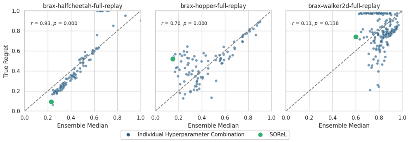
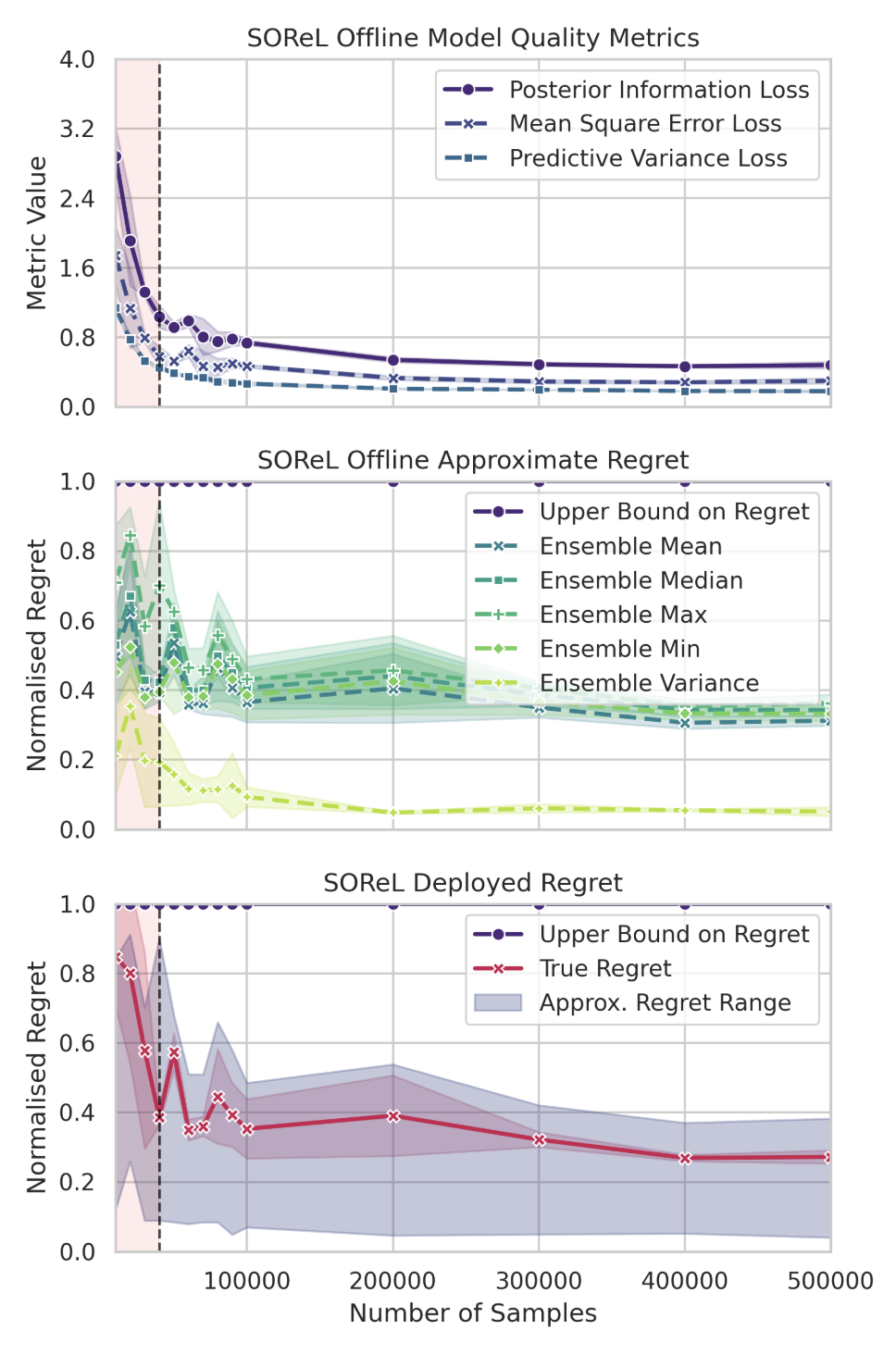
Figure 6: SOReL BAMDP hyperparameter sweeps (tuning set $\phi_{III}$) for 200,000 randomly sampled transitions of the brax datasets. The plots correspond to $\textrm{{\color[rgb]{1,0.23,0.13}$\phi_{III}$}}\leftarrow\operatorname*{arg\,min}_{\textrm{{\color[rgb]{1,0.23,0.13}$\phi_{III}$}}}\text{RegretMetric}(\textrm{{\color[rgb]{0.59,0,0.66}$\phi_{I}$}},\textrm{{\color[rgb]{0,0.6,0}$\phi_{II}$}},\textrm{{\color[rgb]{1,0.23,0.13}$\phi_{III}$}},\mathcal{D}_{N})$ in Algorithm˜1. SOReL selects the BAMDP hyperparameters that yield the lowest approximate regret (green). For Walker2d the high approximate regret for all hyperparameter combinations ($R_{N}>0.6$) suggests that in Algorithm˜1 $R_{N}>\mathcal{R}_{\text{Deploy}}$ has not been satisfied: the practitioner should change the model or approximate inference method to obtain a lower PIL before re-tuning the BAMDP hyperparameters. Alternatively, the practitioner could consider collecting more data - though the high approximate regret highlights the associated risk. While we report the true regret to validate the approach, in practice only the policy with the lowest approximate regret would be deployed.

Figure 7: Simplified version of SOReL on brax-halfcheetah-full-replay. The plot showing only the ensemble median as the approximate regret is given in the main body of the paper. Shaded purple shows the approximate regret range across all the metrics (with varying degrees of conservatism). Shaded red indicates where $\mathcal{E}(\mathcal{D}_{N},\mathcal{M}^{\star})\not\approx\mathcal{V}(\mathcal{D}_{N})$ (for a threshold of $0.25$), and hence the approximate regret may be unreliable. Mean and standard deviation given over 3 seeds.

The only environment for which the world model is sufficiently accurate relative to its discount factor, resulting in a non-trivial upper bound, is pendulum-v1 (Fig.˜8(b)). This is due to two factors: (i) the other environments use a lower discount factor (0.998 vs. 0.995), and (ii) learning accurate world models with low MSE is inherently more challenging in high-dimensional settings. We note that this is a supervised-learning problem, and orthogonal to our line of work.

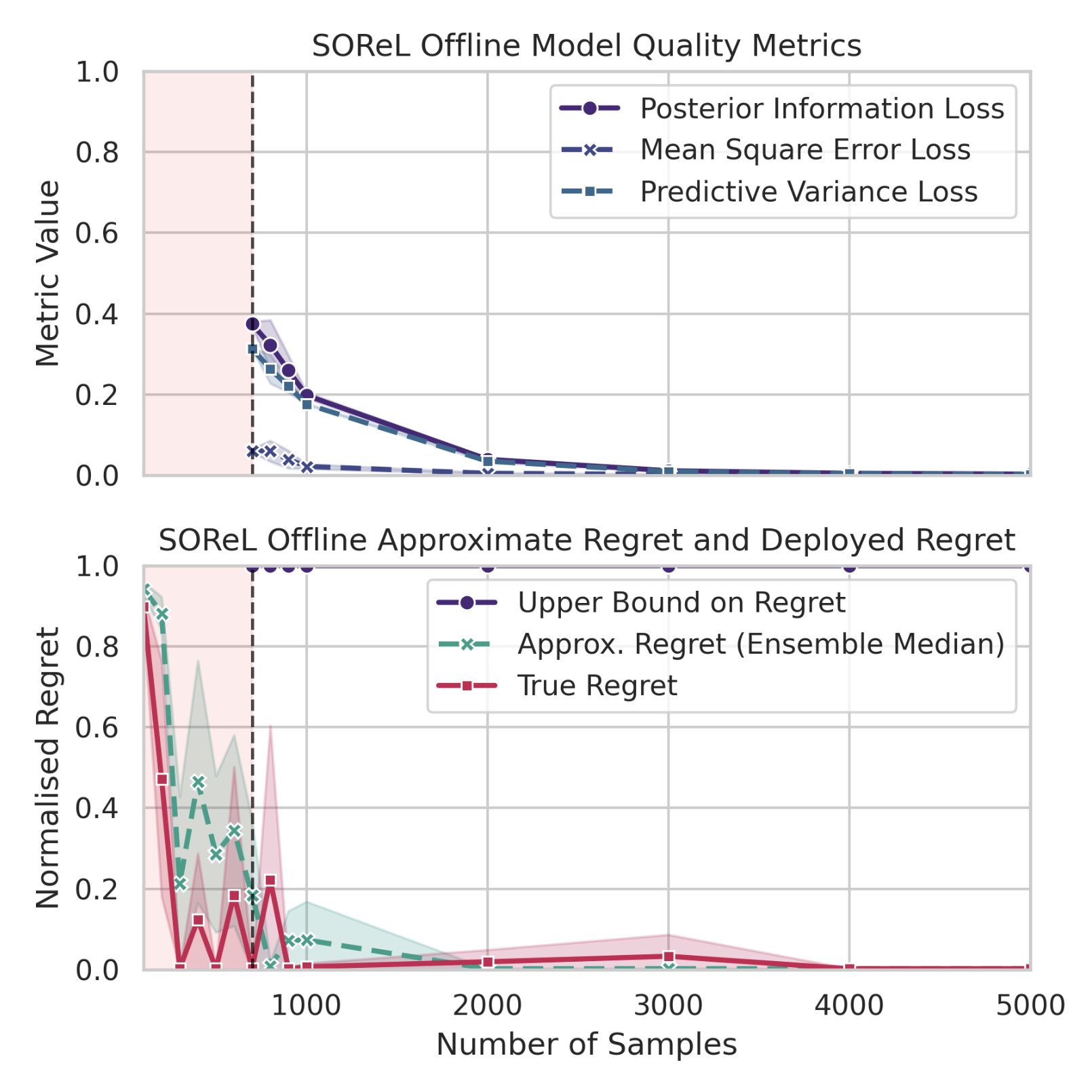
(a) gymnax-cartpole-random-v1

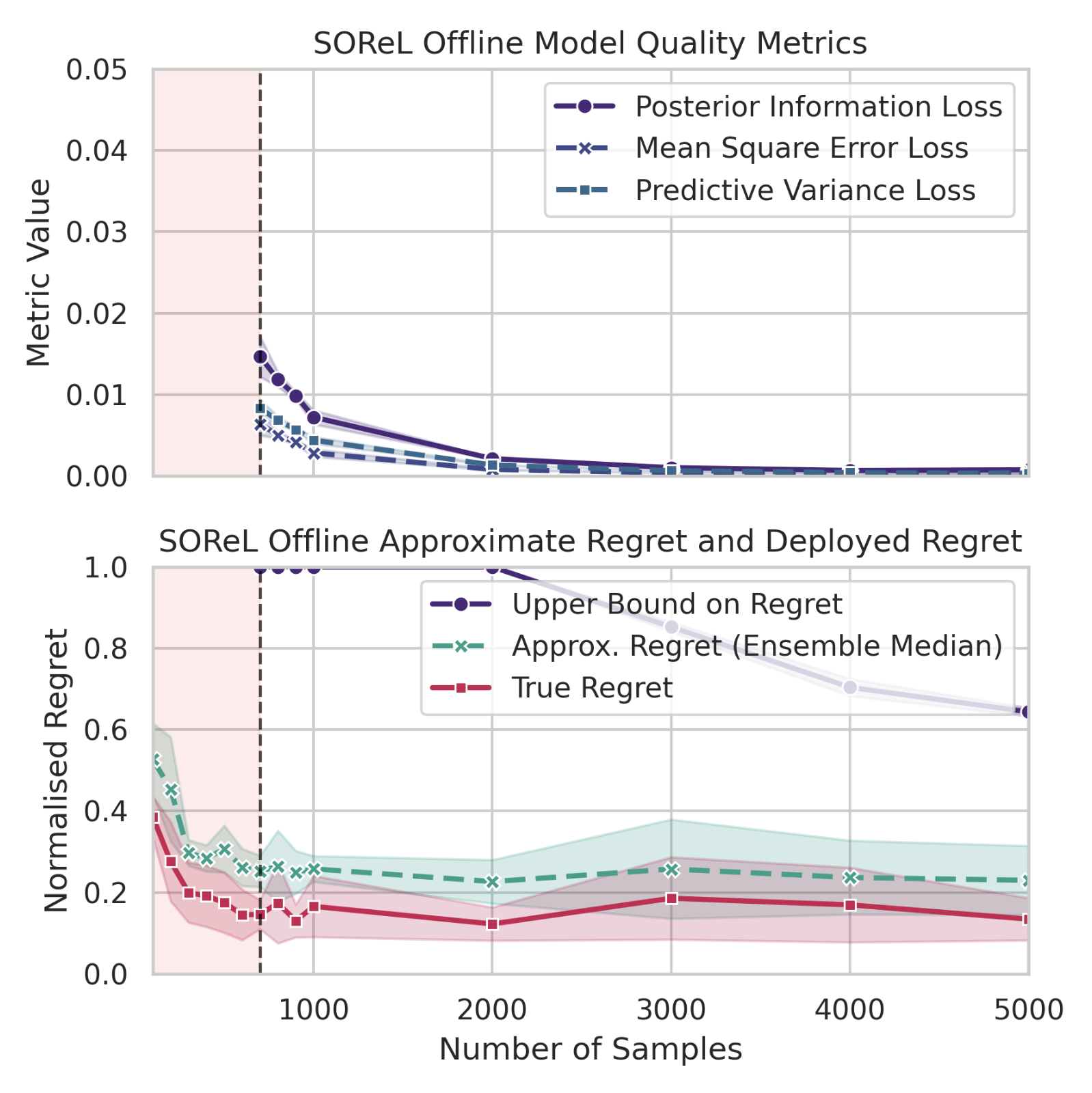
(b) gymnax-pendulum-random-v1

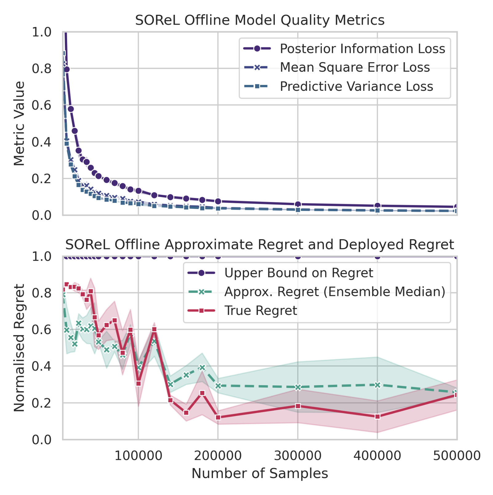
(c) brax-hopper-full-replay

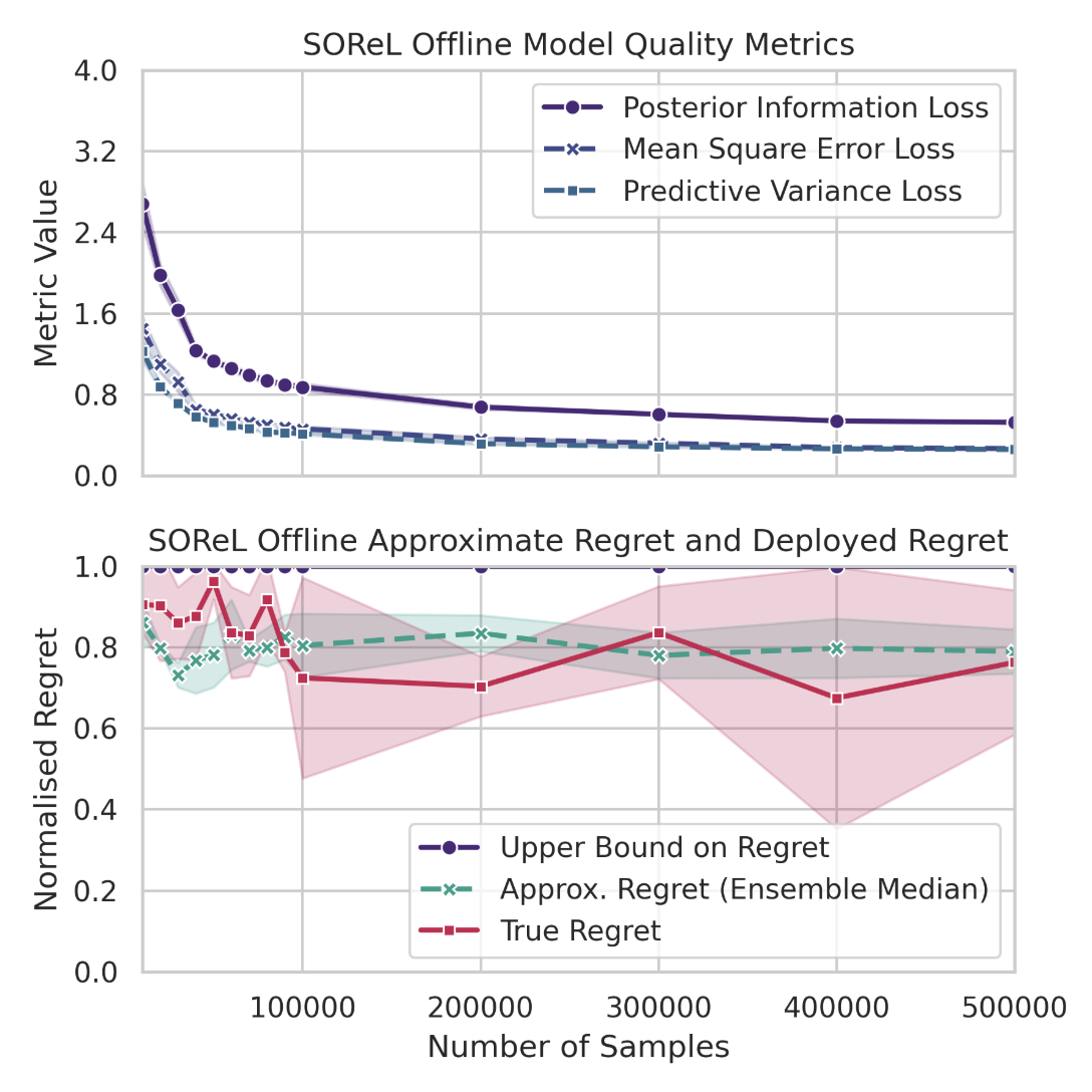
(d) brax-walker2d-full-replay

Figure 8: Simplified version of SOReL applied to various tasks. For the gymnax environments, $N<700$ is shaded red because the PIL is undefined in this region (validation set $<$ batch size): without being able to ensure $\mathcal{E}(\mathcal{D}_{N},\mathcal{M}^{\star})<\approx\mathcal{V}(\mathcal{D}_{N})$ the practitioner would have been unable to determine whether to trust the approximate regret. Mean and standard deviation given over 3 seeds.

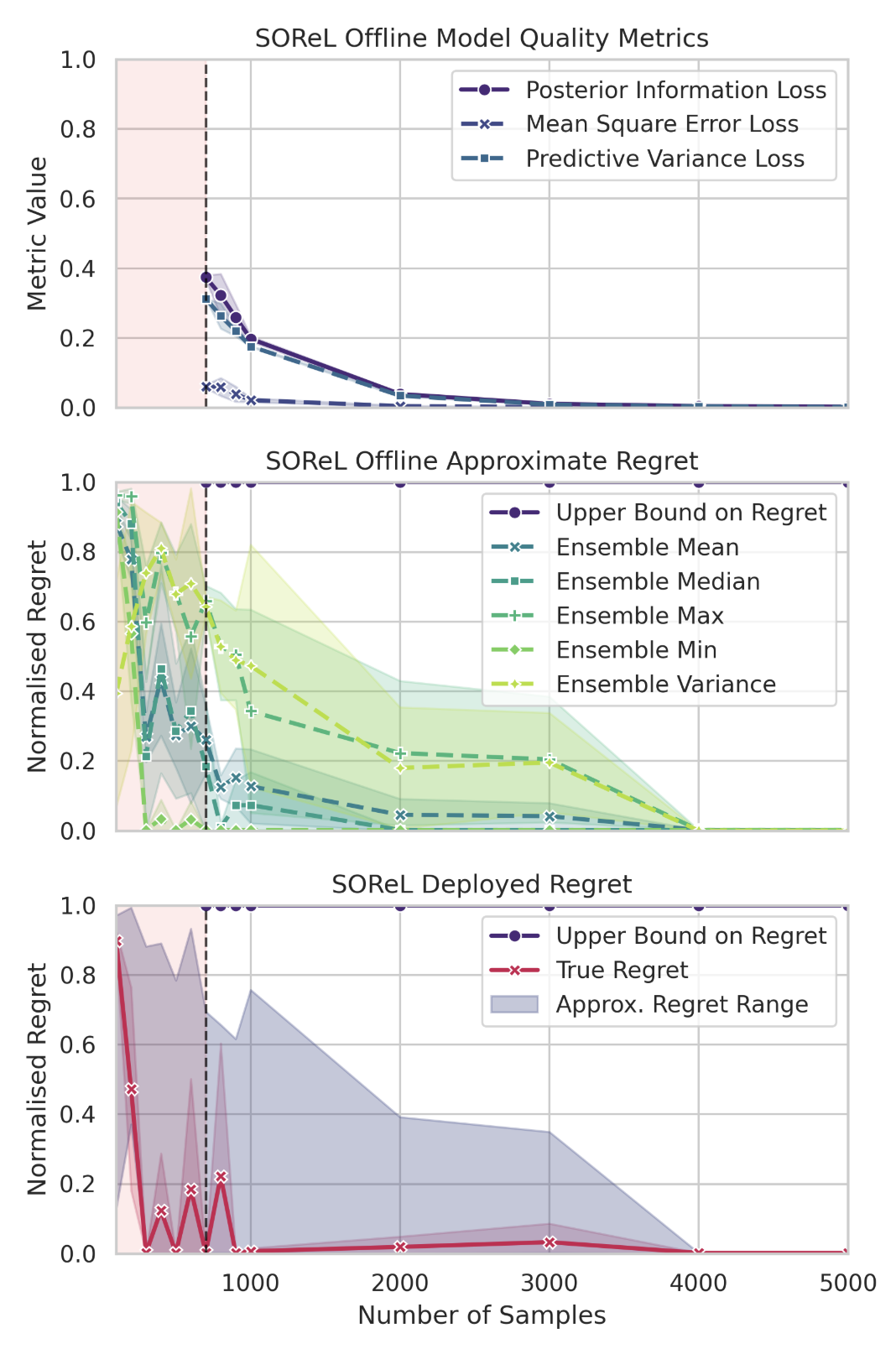
(a) gymnax-cartpole-random-v1

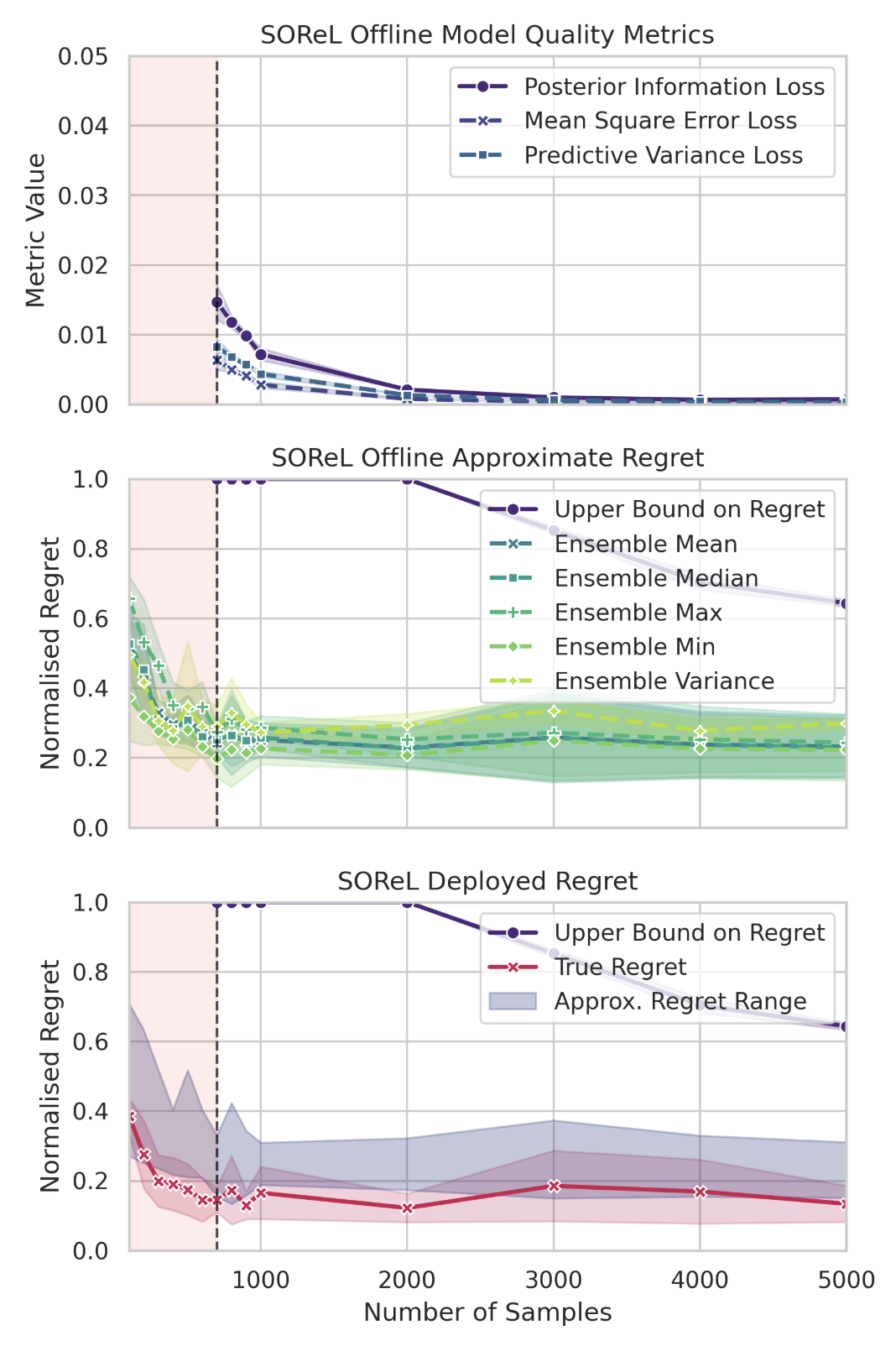
(b) gymnax-pendulum-random-v1

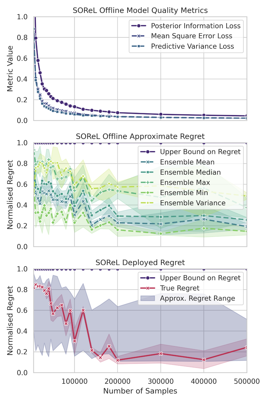
(c) brax-hopper-full-replay

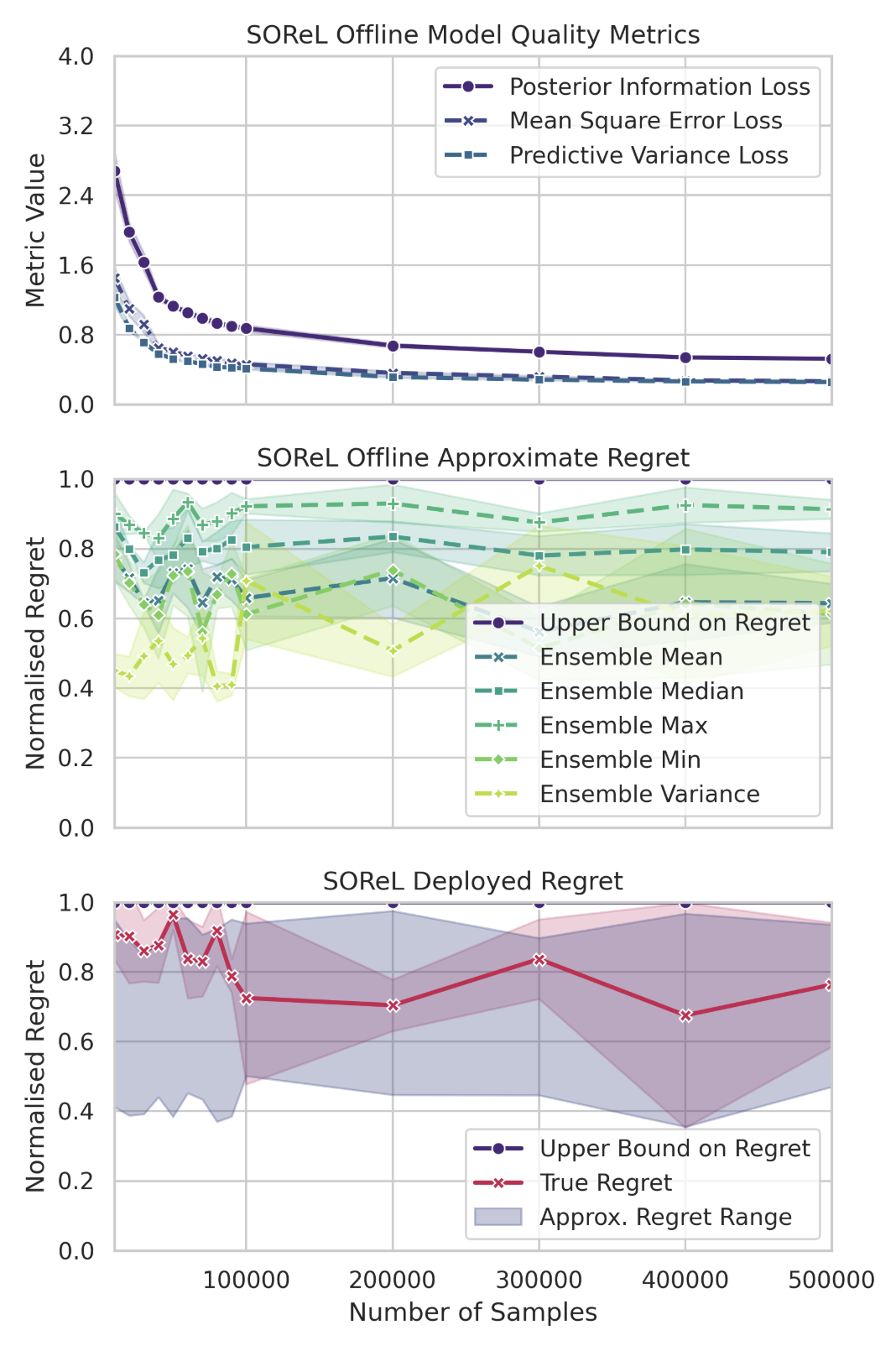
(d) brax-walker2d-full-replay

Figure 9: Simplified version of SOReL applied to various tasks. Shaded purple shows the approximate regret range across all the metrics (with varying degrees of conservatism). For the gymnax environments, $N<700$ is shaded red because the PIL is undefined in this region (validation set $<$ batch size): without being able to ensure $\mathcal{E}(\mathcal{D}_{N},\mathcal{M}^{\star})<\approx\mathcal{V}(\mathcal{D}_{N})$ the practitioner would have been unable to determine whether to trust the approximate regret. Mean and standard deviation given over 3 seeds.

E.2 TOReL

Task		IQL	ReBRAC	MOPO	MOReL
brax- halfcheetah- full-replay	True	$0.203$	$0.312$	$0.403$	$0.751$
	Oracle	$0.186$	$0.089$	$0.133$	$0.641$
	TOReL	0.186	0.089	0.133	0.648
brax- hopper- full-replay	True	$0.550$	$0.534$	$0.558$	$0.575$
	Oracle	$0.377$	$0.070$	$0.082$	$0.243$
	TOReL	0.397	0.070	0.086	0.282
brax- walker- full-replay	True	$0.374$	$0.357$	$0.342$	$0.625$
	Oracle	$0.304$	$0.000$	$0.243$	$0.415$
	TOReL	0.331	0.000	$0.384$	0.554
d4rl- halfcheetah- medium-expert-v2	True	$0.400$	$0.134$	$0.331$	$0.418$
	Oracle	$0.469$	$0.000$	$0.116$	$0.187$
	TOReL	$0.459$	0.036	$0.339$	0.227
d4rl- hopper- medium-v2	True	$0.411$	$0.467$	$0.848$	$0.595$
	Oracle	$0.375$	$0.053$	$0.681$	$0.183$
	TOReL	$0.428$	0.083	0.681	0.327
d4rl- walker2d- medium-replay-v2	True	$0.450$	$0.625$	$0.952$	$1.000$
	Oracle	$0.339$	$0.204$	$0.724$	$1.000$
	TOReL	0.358	0.206	0.724	1.000

Table 2: True, oracle and TOReL regrets across tasks. Bold indicates where TOReL identifies the oracle hyperparameters, while italic indicates where TOReL identifies hyperparameters with a regret lower than the true regret. ReBRAC+TOReL outperforms all algorithms on every dataset.

Task		IQL	ReBRAC	MOPO	MOReL
brax-halfcheetah- full-replay	r	$0.29$	$0.92$	$0.98$	$0.93$
	p	$0.448$	$0.000$	$0.000$	$0.000$
brax-hopper- full-replay	r	$0.18$	$0.98$	$1.00$	$0.98$
	p	$0.635$	$0.000$	$0.00$	$0.000$
brax-walker- full-replay	r	$0.32$	nan	$-0.68$	$0.99$
	p	$0.406$	nan	$0.133$	$0.000$
d4rl-halfcheetah- medium-expert-v2	r	$0.29$	$0.90$	$0.02$	$0.98$
	p	$0.442$	$0.000$	$0.975$	$0.000$
d4rl-hopper- medium-v2	r	$0.29$	$0.98$	$0.98$	$0.94$
	p	$0.443$	$0.000$	$0.000$	$0.000$
d4rl-walker2d- medium-replay-v2	r	$0.65$	$0.79$	$1.00$	$-0.53$
	p	$0.057$	$0.000$	$0.000$	$0.008$

Table 3: Pearson correlation ($r$) and statistical significance ($p$) between TOReL regret metrics and true regrets for different hyperparameter combinations. For two-thirds of the tasks there is statistically significant ($p<0.05$), strong ($r>|0.5|$) positive ($r>0$) correlation (bold). Even where no strong positive correlation is observed (possibly due to limited hyperparameter coverage), the TOReL regret is lower than the true regret averaged over those tasks.

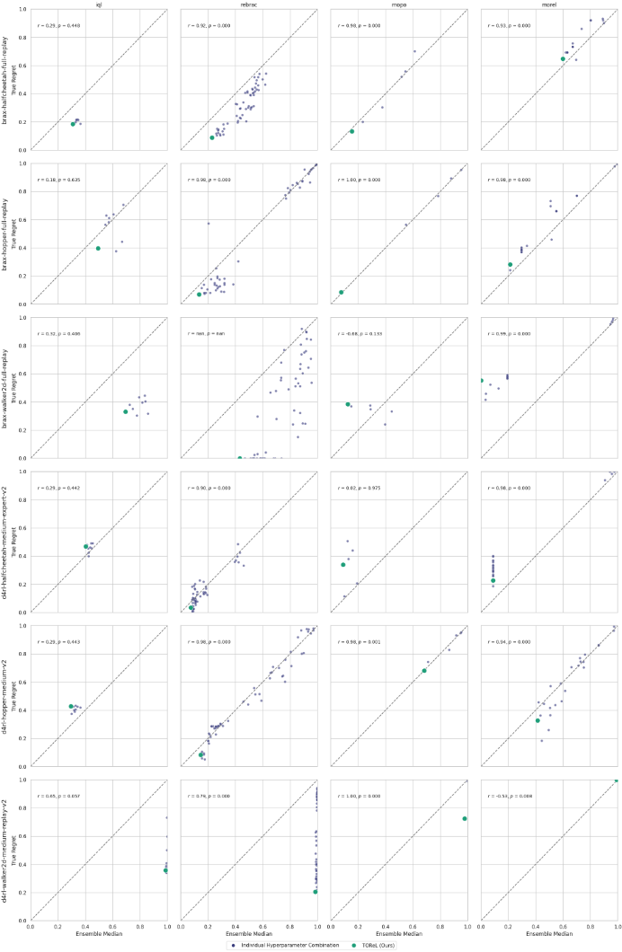
Figure 10: Scatter plots to visualise the positive correlation between the TOReL regret metric and the true regret.

Appendix F Implementation Details

Our implementations of SOReL and TOReL, along with all of the code to reproduce the experiments, are made publicly available with this work.

F.1 Diverse full-replay datasets

As mentioned in Section˜7.1, without a model prior, the offline dataset must include transitions from poor, medium and expert regions of performance. For the brax environments, we collect our own full-replay datasets to ensure that this is the case. We arbitrarily choose the hyperparameters, simply requiring that the agent spends sufficient time in all three regions of performance. The training curves obtained while collecting the offline datasets are given in Figure 11. The gymnax environments are simple enough that collecting a dataset using an ensemble of randomly initialised policies leads to sufficient coverage across all three regions of performance.

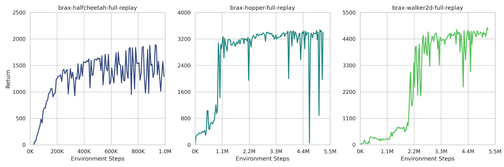
Figure 11: Training curves while collecting the brax full-replay offline datasets. We ensure that the agent spend sufficient time in poor, medium and expert regions of performance such that the offline dataset captures diverse transitions.

F.2 World Model and RP Approximate Inference

To ensure compatibility with Unifloral implementations [Jackson et al., 2025], our world model is a variation of the Gaussian World Model presented in 5.3, but amended to predict the change in state $\Delta\coloneq s^{\prime}-s$ rather than the absolute next state $s^{\prime}$. We also allow the model to characterise its uncertainty with variance functions $\sigma^{2}_{r,\theta}(s,a)$ and $\sigma^{2}_{\Delta,\theta}(s,a)$. The Gaussian reward and state transition models then have the form:

$$P_{R}(s,a,\theta)=\mathcal{N}(r_{\theta}(s,a),\sigma^{2}_{r,\theta}(s,a)),\quad P_{\Delta}(s,a,\theta)=\mathcal{N}(\Delta_{\theta}(s,a),\sigma^{2}_{\Delta,\theta}(s,a)),$$ (223)

with mean reward function $r_{\theta}(s,a)$ and mean state transition function $\Delta_{\theta}(s,a)$, as before. Let $r(s,a,\mathcal{D}_{N})\coloneqq\mathbb{E}_{\theta\sim P_{\Theta}(\mathcal{D}_{N})}\left[r_{\theta}(s,a)\right]$ and $\Delta(s,a,\mathcal{D}_{N})\coloneqq\mathbb{E}_{\theta\sim P_{\Theta}(\mathcal{D}_{N})}\left[\Delta_{\theta}(s,a)\right]$ denote the Bayesian mean reward and state transition functions and $r^{\star}(s,a)$ and ${\Delta^{\star}}(s,a)$ denote the true mean reward and state transition functions. We define the normalised mean squared error between the true and Bayesian mean functions as:

$$\mathcal{E}(\mathcal{D}_{N},\mathcal{M}^{\star})\coloneqq\mathbb{E}_{(s,a)\sim\rho_{\pi}^{\star}}\left[\frac{\lVert r(s,a,\mathcal{D}_{N})-r^{\star}(s,a)\rVert^{2}_{2}}{2\sigma_{r}^{2}(\mathcal{D}_{N})}+\frac{\lVert\Delta(s,a,\mathcal{D}_{N})-{\Delta^{\star}}(s,a)\rVert^{2}_{2}}{2\sigma_{\Delta}^{2}(\mathcal{D}_{N})}\right],$$ (224)

and the normalised predictive variance using the law of total variance as:

$$\mathcal{V}(\mathcal{D}_{N})\coloneqq\ \mathbb{E}_{(s,a)\sim\rho_{\pi}^{\star}}\Bigg{[}\mathbb{E}_{\theta\sim P_{\Theta}(\mathcal{D}_{N})}\Bigg{[}\frac{\lVert r(s,a,\mathcal{D}_{N})-r_{\theta}(s,a)\rVert^{2}_{2}}{2\sigma_{r}^{2}(\mathcal{D}_{N})}+\lVert\sigma_{r,\theta}^{2}(s,a)\rVert^{2}_{2}$$

$$\quad+\frac{\lVert\Delta(s,a,\mathcal{D}_{N})-\Delta_{\theta}(s,a)\rVert^{2}_{2}}{2\sigma_{\Delta}^{2}(\mathcal{D}_{N})}+\lVert\sigma_{\Delta,\theta}^{2}(s,a)\rVert^{2}_{2}\Bigg{]}\Bigg{]},$$ (225)

where $\sigma_{r}^{2}(\mathcal{D}_{N})$ and $\sigma_{\Delta}^{2}(\mathcal{D}_{N})$ denote the variance of the reward and change in state over the offline dataset.

When rolling out sequences of trajectories on which to train our (Bayes-Optimal) policy, we uniformly sample a model from the ensemble of elite models and then sample the transition from the corresponding Gaussian output distribution.

Our ensemble consists of multilayer perceptrons (MLPs) with ReLU activation, which we train using negative log-likelihood loss derived in Section˜C.1. Training the models in parallel allows us to simultaneously optimise maximum and minimum (log) variance parameters for each dimension across the model ensemble, which we use to soft-clamp the (log) variances output by the individual models. This prevents any individual model becoming overly confident or too uncertain in one dimension. All models in our ensemble have identical structure, but are initialised differently using LeCun LeCun et al. [1998] initialisation. The maximum and minimum log-variance terms are initialised at constants. The exact loss function and ensemble dynamics model are the same as the one implemented by Jackson et al. [2025], but we use an Adam optimiser Kingma and Ba [2014] with cosine learning rate schedule rather than constant learning rate. A percentage of the available offline dataset is used as a validation set to calculate the PIL. At the end of training, only a subset of elite models are retained, based on their validation MSE. Although the current implementation uses hard-coded reset and termination conditions during model rollouts, the dynamics model could naturally be extended to learn reset and termination heads. When sampling transitions, we conservatively clip the rewards to remain within the support of the offline dataset distribution.

Hyperparameter	gymnax- cartpole- random-v1	gymnax- pendulum- random-v1	brax- halfcheetah- full-replay	brax- hopper- full-replay	brax- walker2d- full-replay
Num. layers	3	3	3	3	3
Layer Size	200	200	200	200	200
Activation	ReLU	ReLU	ReLU	ReLU	ReLU
Num. Ensemble Models	7	7	7	10	10
Num. Elite Models	5	5	5	8	8
Log Var. Diff. Coeff.	0.01	0.01	0.01	0.01	0.01
Batch Size	64	64	256	256	256
Num. Epochs	400	400	400	400	400
Learning Rate	0.001	0.001	0.001	0.001	0.001
Learning Rate Schedule	cosine	cosine	cosine	cosine	cosine
Final Learning Rate %	10	10	10	10	10
Weight Decay	2.5e-05	2.5e-05	2.5e-05	2.5e-05	2.5e-05
Validation Split	0.1	0.1	0.1	0.1	0.1

Table 4: World model ensemble dynamics hyperparameters.

F.3 BAMDP Solver

We use the RNN-PPO implementation of Lu et al. [2022a], which we amend to be compatible with continuous action spaces. We sweep over the hyperparameters given in Table˜5.

Hyperparameter	Value / Sweep Values
Learning rate	[0.0001, 0.0003]
Anneal learning rate	True
Number of environments	[4, 64, 128, 256, 512]
Steps per environment	[32, 64, 128]
Total timesteps	Set to 500,000, 1,000,000 or 50,000,000
Update epochs	[2, 4, 8]
Number of minibatches	[2, 4, 8, 16]
Discount factor ($\gamma$)	[0.99, 0.995, 0.998]
GAE lambda	[0.8, 0.9, 0.95]
Clip $\epsilon$	[0.2, 0.3]
Entropy coefficient	[0.000, 0.001, 0.010]
Value function coefficient	0.5
Max gradient norm	[0.5, 1.0]
Layer Size	256
Activation function	tanh
RNN size	Set to 64, 128 or 256
Burn-in Percentage	25

Table 5: RNN-PPO hyperparameters swept over.

Hyperparameter	gymnax- cartpole- random-v1	gymnax- pendulum- random-v1	brax- halfcheetah- full-replay	brax- hopper- full-replay	brax- walker2d- full-replay
Learning rate	0.0003	0.0003	0.0003	0.0003	0.0003
Anneal learning rate	True	True	True	True	True
Number of environments	4	128	512	512	512
Steps per environment	128	64	64	32	64
Total timesteps	500,000	1,000,000	50,000,000	50,000,000	50,000,000
Update epochs	4	8	8	2	4
Number of minibatches	4	16	16	8	8
Gamma	0.99	0.99	0.99	0.998	0.995
GAE lambda	0.95	0.95	0.95	0.8	0.95
Clip $\epsilon$	0.2	0.2	0.2	0.3	0.2
Entropy coefficient	0.01	0.003	0.003	0.001	0.001
Value function coefficient	0.5	0.5	0.5	0.5	0.5
Max gradient norm	0.5	0.5	0.5	1.0	0.5
Layer Size	256	256	256	256	256
Activation function	tanh	tanh	tanh	tanh	tanh
RNN size	64	128	256	256	256
Burn-in Percentage	25	25	25	25	25

Table 6: RNN-PPO hyperparameters for gymnax and brax environments. For computational reasons, we sweep over the hyperparameters of each task once, for a fixed dataset size (1000 datapoints for the gymnax tasks and 200,000 datapoints for brax tasks) and choose the hyperparameters corresponding to the lowest approximate regret, which we then use to train the policy of all other dataset sizes. Ideally, we would sweep over all hyperparameters for each dataset size.

F.4 ORL Implementations

We use Jackson et al. [2025]’s implementations of the ORL algorithms. We use their default hyperparameters and sweep over their suggested hyperparameters, which we summarise in Table˜7.

	Hyperparameter	Value / Sweep Values
Generic Optimisation	Discount factor $\gamma$	0.99
	Polyak averaging coefficient	0.005
IQL	Learning rate	0.0003
	Batch size	256
	Beta	[0.5, 3.0, 10.0]
	$\tau$ (expectile)	[0.5, 0.7, 0.9]
	Advantage clip	100.0
ReBRAC	Learning rate	0.001
	Batch size	1024
	Critic BC coefficient	[0, 0.0001, 0.0005, 0.001, 0.005, 0.01, 0.1]
	Actor BC coefficient	[0.0005, 0.001, 0.002, 0.003, 0.03, 0.1, 0.3, 1.0]
	Critic layer norm	true
	Actor layer norm	false
	Observation normalization	false
	Noise clip	0.5
	Policy noise	0.2
	Num critic updates per step	2
MOPO	Learning rate	0.0001
	Batch size	256
	Model retain epochs	5
	Number of critics	10
	Rollout batch size	50000
	Rollout interval	1000
	Rollout length	[1, 3, 5]
	Dataset sample ratio	0.05
	Step penalty coefficient	[1.0, 5.0]
MOReL	Learning rate	0.0001
	Batch size	256
	Model retain epochs	5
	Number of critics	10
	Rollout batch size	50000
	Rollout interval	1000
	Rollout length	5
	Dataset sample ratio	0.01
	Threshold coefficient	[0, 5, 10, 15, 20, 25]
	Termination penalty offset	[-30, -50, -100, -200]

Table 7: Hyperparameters and sweep ranges for IQL, ReBRAC, MOPO, and MOReL.

For the sample efficiency experiments in Fig.˜5, we use the default UCB bandit-based hyperparameter-tuning algorithm hyperparameters. We rescale the regret into a score to be maximised, normalised between 0 and 100 ($100\cdot(1-\text{regret})$), enabling fair comparison and compatibility with the algorithm.

F.5 Regret Normalisation

We normalise the regret using the (known) minimum and maximum returns ($R_{min}$ and $R_{max}$) that an online-learnt policy would achieve in the true environment. In the absence of access to these values, we suggest estimating $R_{max}$ or $R_{min}$ as $\frac{r_{min}}{1-\gamma}$ and $\frac{r_{max}}{1-\gamma}$ respectively, where $r_{min}$ and $r_{max}$ denote the 2.5th and 97.5th percentiles of episode rewards in the offline dataset. These thresholds are suggested to avoid unrealistic assumptions, such as that the best possible policy consistently receives the 100th percentile reward at every time step. Such unrealistic assumptions may significantly distort results, especially in reward distributions with heavy tails where an inflated $R_{max}-R_{min}$ would compress the true and expected regrets.

	gymnax- cart pole- random- v1	gymnax- pend ulum- random- v1	brax- half cheetah- full- replay	brax- hop per- full- replay	brax- walker 2d full- replay	d4rl- halfcheetah medium- expert- v2	d4rl- hopper med ium- v2	d4rl- walker2d medium- replay- v2
$r_{\text{min}}$	0	-13.3	-0.50	0.00	0.00	-0.28	-0.20	0.00
$r_{\text{max}}$	1	-0.2	3.50	3.50	3.50	12.14	3.23	4.59
$P_{2.5}$	1	-13.2	-0.84	1.08	0.01	1.99	1.25	-0.19
$P_{97.5}$	1	-0.16	3.44	4.34	5.65	12.39	4.73	4.92

Table 8: Top half of table: for the gymnax and brax tasks, we define $r_{min}$ and $r_{max}$ using approximate known minimum and maximum returns Jesson et al. [2024], and dividing by the episode length. For the D4RL tasks, we divide the given D4RL minimum and maximum reference scores by the episode length to find $r_{min}$ and $r_{max}$. Bottom half of table: the suggested normalisation values if expert and random scores were unknown, and determined using the $95^{th}$ percentile of the offline dataset. Based on the above datasets, for all datasets apart from cartpole-v1, normalisation using the $95^{th}$ percentile approximation would lead to a more conservative approximate regret. We note that as long as we use the same normalisation constants for both the approximate and true regrets, the absolute value of the normalisation constants is arbitrary. cartpole-v1 is an exception, as the reward is constant for each step (episode returns vary only due to early termination).

We calculate the infinite horizon discounted return from the finite horizon discounted return as follows:

$$R_{inf}=R_{fin}\cdot\left(1+\frac{\gamma^{s}}{1-\gamma^{s}}\right),$$ (226)

where $s$ represents the maximum number of episode steps. The normalised regret is then calculated from the infinite horizon discounted return using:

$$\text{Regret}=\frac{R_{max}-R_{inf}}{R_{max}-R_{min}}.$$ (227)

F.6 Experiment Compute Resources

All of our experiments were run within a week using four L40S GPUs.

References

• Aitchison (1975) J. Aitchison. Goodness of prediction fit. Biometrika, 62(3):547–554, 1975. ISSN 00063444, 14643510. URL http://www.jstor.org/stable/2335509.
• Alaa and van der Schaar (2018) Ahmed M. Alaa and Mihaela van der Schaar. Bayesian nonparametric causal inference: Information rates and learning algorithms. IEEE Journal of Selected Topics in Signal Processing, 12(5):1031–1046, 2018. doi: 10.1109/JSTSP.2018.2848230.
• An et al. (2021) Gaon An, Seungyong Moon, Jang-Hyun Kim, and Hyun Oh Song. Uncertainty-based offline reinforcement learning with diversified q-ensemble. In M. Ranzato, A. Beygelzimer, Y. Dauphin, P.S. Liang, and J. Wortman Vaughan, editors, Advances in Neural Information Processing Systems, volume 34, pages 7436–7447. Curran Associates, Inc., 2021. URL https://proceedings.neurips.cc/paper_files/paper/2021/file/3d3d286a8d153a4a58156d0e02d8570c-Paper.pdf.
• Aslan (2006) Mihaela Aslan. Asymptotically minimax bayes predictive densities. The Annals of Statistics, 34(6):2921–2938, 2006. ISSN 00905364. URL http://www.jstor.org/stable/25463538.
• Ball et al. (2021) Philip J Ball, Cong Lu, Jack Parker-Holder, and Stephen Roberts. Augmented world models facilitate zero-shot dynamics generalization from a single offline environment. In Marina Meila and Tong Zhang, editors, Proceedings of the 38th International Conference on Machine Learning, volume 139 of Proceedings of Machine Learning Research, pages 619–629. PMLR, 18–24 Jul 2021. URL https://proceedings.mlr.press/v139/ball21a.html.
• Barron (1999) Andrew R Barron. Information-theoretic characterization of bayes performance and the choice of priors in parametric and nonparametric problems. In Bayesian Statistics 6: Proceedings of the Sixth Valencia International Meeting June 6-10, 1998. Oxford University Press, 08 1999. ISBN 9780198504856. doi: 10.1093/oso/9780198504856.003.0002. URL https://doi.org/10.1093/oso/9780198504856.003.0002.
• Barron (1988) A.R. Barron. The Exponential Convergence of Posterior Probabilities with Implications for Bayes Estimators of Density Functions. Department of Statistics, University of Illinois, 1988. URL https://books.google.co.uk/books?id=8raEnQAACAAJ.
• Bass (2013) R.F. Bass. Real Analysis for Graduate Students, chapter 21. Createspace Ind Pub, 2013. ISBN 9781481869140. URL https://books.google.co.uk/books?id=s6mVlgEACAAJ.
• Beck et al. (2024) Jacob Beck, Risto Vuorio, Evan Zheran Liu, Zheng Xiong, Luisa Zintgraf, Chelsea Finn, and Shimon Whiteson. A survey of meta-reinforcement learning, 2024. URL https://arxiv.org/abs/2301.08028.
• Bellman (1956) Richard Bellman. A problem in the sequential design of experiments. Sankhyā: The Indian Journal of Statistics (1933-1960), 16(3/4):221–229, 1956. ISSN 00364452. URL http://www.jstor.org/stable/25048278.
• Bellman (1958) Richard Bellman. Dynamic programming and stochastic control processes. Information and Control, 1(3):228–239, 1958. ISSN 0019-9958. doi: https://doi.org/10.1016/S0019-9958(58)80003-0. URL https://www.sciencedirect.com/science/article/pii/S0019995858800030.
• Bilodeau et al. (2021) Blair Bilodeau, Dylan J. Foster, and Daniel M. Roy. Minimax rates for conditional density estimation via empirical entropy. The Annals of Statistics, 2021. URL https://api.semanticscholar.org/CorpusID:237592759.
• Birnbaum (1962) Allan Birnbaum. On the foundations of statistical inference. Journal of the American Statistical Association, 57(298):269–306, 1962. doi: 10.1080/01621459.1962.10480660. URL https://www.tandfonline.com/doi/abs/10.1080/01621459.1962.10480660.
• Bretagnolle and Huber (1978) J. L. Bretagnolle and Catherine Huber. Estimation des densités: risque minimax. Zeitschrift für Wahrscheinlichkeitstheorie und Verwandte Gebiete, 47:119–137, 1978. URL https://api.semanticscholar.org/CorpusID:122597694.
• Chen et al. (2024) Jiayu Chen, Wentse Chen, and Jeff Schneider. Bayes adaptive monte carlo tree search for offline model-based reinforcement learning, 2024. URL https://arxiv.org/abs/2410.11234.
• Ciosek et al. (2020) Kamil Ciosek, Vincent Fortuin, Ryota Tomioka, Katja Hofmann, and Richard Turner. Conservative uncertainty estimation by fitting prior networks. In Eighth International Conference on Learning Representations, 04 2020.
• Clarke and Barron (1990) B.S. Clarke and A.R. Barron. Information-theoretic asymptotics of bayes methods. IEEE transactions on information theory, 36(3):453–471, 1990. ISSN 0018-9448.
• Doob (1949) J. L. Doob. Application of the theory of martingales. In Le calcul des probabilités et ses applications [The calculus of probabilities and its applications], number 13 in CNRS International Colloquia, pages 23–27. Centre National de la Recherche Scientifique, Paris, 1949. (Lyon, France, 28 June–3 July 1948). MR:33460. Zbl:0041.45101.
• Drake (1962) Alvin Drake. Observation of a markov process through a noisy channel. PhD Thesis, 1962.
• Duan et al. (1987) Yan Duan, John Schulman, Xi Chen, Peter Bartlett, Ilya Sutskever, and Peter Abbeel. Fast reinforcement learning via slow reinforcement learning. 1987.
• Duff (2002) Michael O’Gordon Duff. Optimal Learning: Computational Procedures for Bayes-Adaptive Markov Decision Processes. PhD thesis, 2002. AAI3039353.
• Fellows et al. (2024) Mattie Fellows, Brandon Kaplowitz, Christian Schroeder de Witt, and Shimon Whiteson. Bayesian exploration networks. In ICML, 2024.
• Fu et al. (2020) Justin Fu, Aviral Kumar, Ofir Nachum, George Tucker, and Sergey Levine. D4rl: Datasets for deep data-driven reinforcement learning, 2020.
• Fujimoto and Gu (2021) Scott Fujimoto and Shixiang (Shane) Gu. A minimalist approach to offline reinforcement learning. In M. Ranzato, A. Beygelzimer, Y. Dauphin, P.S. Liang, and J. Wortman Vaughan, editors, Advances in Neural Information Processing Systems, volume 34, pages 20132–20145. Curran Associates, Inc., 2021. URL https://proceedings.neurips.cc/paper_files/paper/2021/file/a8166da05c5a094f7dc03724b41886e5-Paper.pdf.
• Gandenberger (2015) Greg Gandenberger. A new proof of the likelihood principle. The British Journal for the Philosophy of Science, 66(3):475–503, 2015. doi: 10.1093/bjps/axt039. URL https://doi.org/10.1093/bjps/axt039.
• Guez et al. (2012) Arthur Guez, David Silver, and Peter Dayan. Efficient bayes-adaptive reinforcement learning using sample-based search. In F. Pereira, C. J. C. Burges, L. Bottou, and K. Q. Weinberger, editors, Advances in Neural Information Processing Systems, volume 25. Curran Associates, Inc., 2012. URL https://proceedings.neurips.cc/paper/2012/file/35051070e572e47d2c26c241ab88307f-Paper.pdf.
• Guez et al. (2013) Arthur Guez, David Silver, and Peter Dayan. Scalable and efficient bayes-adaptive reinforcement learning based on monte-carlo tree search. Journal of Artificial Intelligence Research, 48:841–883, 10 2013. doi: 10.1613/jair.4117.
• Guez et al. (2014) Arthur Guez, Nicolas Heess, David Silver, and Peter Dayan. Bayes-adaptive simulation-based search with value function approximation. In Z. Ghahramani, M. Welling, C. Cortes, N. Lawrence, and K.Q. Weinberger, editors, Advances in Neural Information Processing Systems, volume 27. Curran Associates, Inc., 2014. URL https://proceedings.neurips.cc/paper_files/paper/2014/file/74d863ca4a12ccca50a754a3b277dbf7-Paper.pdf.
• Hartigan (1998) J. A. Hartigan. The maximum likelihood prior. The Annals of statistics, 26(6):2083–2103, 1998. ISSN 0090-5364.
• Jackson et al. (2025) Matthew Thomas Jackson, Uljad Berdica, Jarek Liesen, Shimon Whiteson, and Jakob Nicolaus Foerster. A clean slate for offline reinforcement learning. arXiv preprint arXiv:2504.11453, 2025.
• Jesson et al. (2024) A Jesson, C Lu, N Beltran-Velez, A Filos, J Foerster, and Y Gal. Relu to the rescue: Improve your on-policy actor-critic with positive advantages. 2024.
• Kaelbling et al. (1998) Leslie Pack Kaelbling, Michael L. Littman, and Anthony R. Cassandra. Planning and acting in partially observable stochastic domains. Artif. Intell., 101(1–2):99–134, may 1998. ISSN 0004-3702.
• Kass et al. (1990) Robert E Kass, Luke Thierney, and Joeseph B Kadane. The validity of posterior expansions based on laplace’s method. Bayesian and Likelihood Methods in Statistics and Economics, pages 473–488, 1990. URL https://www.stat.cmu.edu/˜kass/papers/validity.pdf.
• Kidambi et al. (2020) Rahul Kidambi, Aravind Rajeswaran, Praneeth Netrapalli, and Thorsten Joachims. Morel: Model-based offline reinforcement learning. In H. Larochelle, M. Ranzato, R. Hadsell, M.F. Balcan, and H. Lin, editors, Advances in Neural Information Processing Systems, volume 33, pages 21810–21823. Curran Associates, Inc., 2020. URL https://proceedings.neurips.cc/paper_files/paper/2020/file/f7efa4f864ae9b88d43527f4b14f750f-Paper.pdf.
• Kingma and Ba (2014) Diederik P Kingma and Jimmy Ba. Adam: A method for stochastic optimization. arXiv preprint arXiv:1412.6980, 2014.
• Kleijn and van der Vaart (2012) B.J.K. Kleijn and A.W. van der Vaart. The Bernstein-Von-Mises theorem under misspecification. Electronic Journal of Statistics, 6(none):354 – 381, 2012. doi: 10.1214/12-EJS675. URL https://doi.org/10.1214/12-EJS675.
• KOMAKI (1996) FUMIYASU KOMAKI. On asymptotic properties of predictive distributions. Biometrika, 83(2):299–313, 06 1996. ISSN 0006-3444. doi: 10.1093/biomet/83.2.299. URL https://doi.org/10.1093/biomet/83.2.299.
• Kostrikov et al. (2021) Ilya Kostrikov, Ashvin Nair, and Sergey Levine. Offline reinforcement learning with implicit q-learning. CoRR, abs/2110.06169, 2021. URL https://arxiv.org/abs/2110.06169.
• Krige (1951) Danie G. Krige. A statistical approach to some basic mine valuation problems on the witwatersand. Journal of the Chemical, Metallurgical and Mining Society of South Africa, 52:119–139, 1951.
• Kumar et al. (2020) Aviral Kumar, Aurick Zhou, George Tucker, and Sergey Levine. Conservative q-learning for offline reinforcement learning. In H. Larochelle, M. Ranzato, R. Hadsell, M.F. Balcan, and H. Lin, editors, Advances in Neural Information Processing Systems, volume 33, pages 1179–1191. Curran Associates, Inc., 2020. URL https://proceedings.neurips.cc/paper_files/paper/2020/file/0d2b2061826a5df3221116a5085a6052-Paper.pdf.
• Lange et al. (2012) Sascha Lange, Thomas Gabel, and Martin Riedmiller. Batch Reinforcement Learning, pages 45–73. Springer Berlin Heidelberg, Berlin, Heidelberg, 2012. ISBN 978-3-642-27645-3. doi: 10.1007/978-3-642-27645-3_2. URL https://doi.org/10.1007/978-3-642-27645-3_2.
• Le Cam (1953) Lucien Le Cam. On some asymptotic properties of maximum likelihood estimates and related bayes’ estimates. volume 1, pages 277–300, 1953.
• LeCun et al. (1998) Yann LeCun, Leon Bottou, Genevieve B Orr, and Klaus-Robert Mueller. Efficient backprop. In Neural Networks: Tricks of the Trade, pages 9–50. Springer, 1998.
• Levine et al. (2020) Sergey Levine, Aviral Kumar, George Tucker, and Justin Fu. Offline reinforcement learning: Tutorial, review, and perspectives on open problems, 2020. URL https://arxiv.org/abs/2005.01643.
• Lindley (1980) D. V. Lindley. Approximate bayesian methods. Trabajos de Estadistica Y de Investigacion Operativa, 31(1):223–245, 1980.
• Lu et al. (2022a) Chris Lu, Jakub Kuba, Alistair Letcher, Luke Metz, Christian Schroeder de Witt, and Jakob Foerster. Discovered policy optimisation. Advances in Neural Information Processing Systems, 35:16455–16468, 2022a.
• Lu et al. (2022b) Cong Lu, Philip Ball, Jack Parker-Holder, Michael Osborne, and Stephen J. Roberts. Revisiting design choices in offline model based reinforcement learning. In International Conference on Learning Representations, 2022b. URL https://openreview.net/forum?id=zz9hXVhf40.
• Martin (1967) J. J. Martin. Bayesian decision problems and Markov chains [by] J. J. Martin. Wiley New York, 1967.
• Murphy (2024) Kevin Murphy. Reinforcement learning: An overview, 2024. URL https://arxiv.org/abs/2412.05265.
• Osband and Van Roy (2017) Ian Osband and Benjamin Van Roy. Why is posterior sampling better than optimism for reinforcement learning? In Doina Precup and Yee Whye Teh, editors, Proceedings of the 34th International Conference on Machine Learning, volume 70 of Proceedings of Machine Learning Research, pages 2701–2710. PMLR, 06–11 Aug 2017. URL https://proceedings.mlr.press/v70/osband17a.html.
• Osband et al. (2018) Ian Osband, John Aslanides, and Albin Cassirer. Randomized prior functions for deep reinforcement learning. In S. Bengio, H. Wallach, H. Larochelle, K. Grauman, N. Cesa-Bianchi, and R. Garnett, editors, Advances in Neural Information Processing Systems 31, pages 8617–8629. Curran Associates, Inc., 2018. URL http://papers.nips.cc/paper/8080-randomized-prior-functions-for-deep-reinforcement-learning.pdf.
• Paine et al. (2020) Tom Le Paine, Cosmin Paduraru, Andrea Michi, Çaglar Gülçehre, Konrad Zolna, Alexander Novikov, Ziyu Wang, and Nando de Freitas. Hyperparameter selection for offline reinforcement learning. CoRR, abs/2007.09055, 2020. URL https://arxiv.org/abs/2007.09055.
• Petersen and Pedersen (2012) K. B. Petersen and M. S. Pedersen. The matrix cookbook, nov 2012. URL http://localhost/pubdb/p.php?3274. Version 20121115.
• Puterman (1994) Martin L. Puterman. Markov Decision Processes: Discrete Stochastic Dynamic Programming. John Wiley & Sons, Inc., USA, 1st edition, 1994. ISBN 0471619779.
• Rasmussen and Williams (2006) Carl Edward Rasmussen and Christopher K. I. Williams. Gaussian Processes for Machine Learning. The MIT Press, 2006. URL https://gaussianprocess.org/gpml/.
• Roberts and Rosenthal (2004) Gareth O. Roberts and Jeffrey S. Rosenthal. General state space Markov chains and MCMC algorithms. Probability Surveys, 1(none):20 – 71, 2004. doi: 10.1214/154957804100000024. URL https://doi.org/10.1214/154957804100000024.
• Schulman et al. (2017) John Schulman, Filip Wolski, Prafulla Dhariwal, Alec Radford, and Oleg Klimov. Proximal policy optimization algorithms. CoRR, abs/1707.06347, 2017.
• Sims et al. (2024) Anya Sims, Cong Lu, Jakob Nicolaus Foerster, and Yee Whye Teh. The edge-of-reach problem in offline model-based reinforcement learning. In The Thirty-eighth Annual Conference on Neural Information Processing Systems, 2024. URL https://openreview.net/forum?id=3dn1hINA6o.
• Smallwood and Sondik (1973) Richard D. Smallwood and Edward J. Sondik. The optimal control of partially observable markov processes over a finite horizon. Operations Research, 21(5):1071–1088, 1973. ISSN 0030364X, 15265463. URL http://www.jstor.org/stable/168926.
• Smith et al. (2023) Matthew Smith, Lucas Maystre, Zhenwen Dai, and Kamil Ciosek. A strong baseline for batch imitation learning, 2023. URL https://arxiv.org/abs/2302.02788.
• Sriperumbudur et al. (2009) Bharath K. Sriperumbudur, Kenji Fukumizu, Arthur Gretton, Bernhard Scholkopf, and Gert R. G. Lanckriet. On integral probability metrics, $\phi$-divergences and binary classification. arXiv: Information Theory, 2009. URL https://api.semanticscholar.org/CorpusID:14114329.
• Sun et al. (2023) Yihao Sun, Jiaji Zhang, Chengxing Jia, Haoxin Lin, Junyin Ye, and Yang Yu. Model-Bellman inconsistency for model-based offline reinforcement learning. In Andreas Krause, Emma Brunskill, Kyunghyun Cho, Barbara Engelhardt, Sivan Sabato, and Jonathan Scarlett, editors, Proceedings of the 40th International Conference on Machine Learning, volume 202 of Proceedings of Machine Learning Research, pages 33177–33194. PMLR, 23–29 Jul 2023. URL https://proceedings.mlr.press/v202/sun23q.html.
• Sutton and Barto (2018) Richard S. Sutton and Andrew G. Barto. Reinforcement Learning: An Introduction. The MIT Press, second edition, 2018. URL http://incompleteideas.net/book/the-book-2nd.html.
• Szepesvári (2010) Csaba Szepesvári. Algorithms for Reinforcement Learning. Synthesis Lectures on Artificial Intelligence and Machine Learning, 4(1):1–103, 2010. ISSN 1939-4608. doi: 10.2200/S00268ED1V01Y201005AIM009. URL http://www.morganclaypool.com/doi/abs/10.2200/S00268ED1V01Y201005AIM009.
• Tarasov et al. (2023) Denis Tarasov, Vladislav Kurenkov, Alexander Nikulin, and Sergey Kolesnikov. Revisiting the minimalist approach to offline reinforcement learning. In Thirty-seventh Conference on Neural Information Processing Systems, 2023. URL https://openreview.net/forum?id=vqGWslLeEw.
• Tierney and Kadane (1986) Luke Tierney and Joseph B. Kadane. Accurate approximations for posterior moments and marginal densities. Journal of the American Statistical Association, 81(393):82–86, 1986. ISSN 0162-1459.
• Tierney et al. (1989) Luke Tierney, Robert E. Kass, and Joseph B. Kadane. Fully exponential laplace approximations to expectations and variances of nonpositive functions. Journal of the American Statistical Association, 84(407):710–716, 1989. ISSN 0162-1459.
• Vaart (1998) A. W. van der Vaart. Bayes Procedures, page 138–152. Cambridge Series in Statistical and Probabilistic Mathematics. Cambridge University Press, 1998. doi: 10.1017/CBO9780511802256.011.
• van der Vaart and van Zanten (2011) Aad van der Vaart and Harry van Zanten. Information rates of nonparametric gaussian process methods. J. Mach. Learn. Res., 12(null):2095–2119, July 2011. ISSN 1532-4435.
• Wang et al. (2022) Han Wang, Archit Sakhadeo, Adam M White, James M Bell, Vincent Liu, Xutong Zhao, Puer Liu, Tadashi Kozuno, Alona Fyshe, and Martha White. No more pesky hyperparameters: Offline hyperparameter tuning for RL. Transactions on Machine Learning Research, 2022. ISSN 2835-8856. URL https://openreview.net/forum?id=AiOUi3440V.
• Wang et al. (2020) Ruosong Wang, Dean P. Foster, and Sham M. Kakade. What are the statistical limits of offline rl with linear function approximation?, 2020. URL https://arxiv.org/abs/2010.11895.
• Wiener (1923) Norbert Wiener. Differential-space. Journal of Mathematics and Physics, 2(1-4):131–174, 1923. doi: https://doi.org/10.1002/sapm192321131. URL https://onlinelibrary.wiley.com/doi/abs/10.1002/sapm192321131.
• Yang and Barron (1999) Yuhong Yang and Andrew Barron. Information-theoretic determination of minimax rates of convergence. The Annals of Statistics, 27(5):1564 – 1599, 1999. doi: 10.1214/aos/1017939142. URL https://doi.org/10.1214/aos/1017939142.
• Yu et al. (2020) Tianhe Yu, Garrett Thomas, Lantao Yu, Stefano Ermon, James Y Zou, Sergey Levine, Chelsea Finn, and Tengyu Ma. Mopo: Model-based offline policy optimization. In H. Larochelle, M. Ranzato, R. Hadsell, M.F. Balcan, and H. Lin, editors, Advances in Neural Information Processing Systems, volume 33, pages 14129–14142. Curran Associates, Inc., 2020. URL https://proceedings.neurips.cc/paper_files/paper/2020/file/a322852ce0df73e204b7e67cbbef0d0a-Paper.pdf.
• Yu et al. (2021) Tianhe Yu, Aviral Kumar, Rafael Rafailov, Aravind Rajeswaran, Sergey Levine, and Chelsea Finn. Combo: Conservative offline model-based policy optimization. In M. Ranzato, A. Beygelzimer, Y. Dauphin, P.S. Liang, and J. Wortman Vaughan, editors, Advances in Neural Information Processing Systems, volume 34, pages 28954–28967. Curran Associates, Inc., 2021. URL https://proceedings.neurips.cc/paper_files/paper/2021/file/f29a179746902e331572c483c45e5086-Paper.pdf.
• Zhang et al. (2021) Baohe Zhang, Raghu Rajan, Luis Pineda, Nathan Lambert, André Biedenkapp, Kurtland Chua, Frank Hutter, and Roberto Calandra. On the importance of hyperparameter optimization for model-based reinforcement learning. In Arindam Banerjee and Kenji Fukumizu, editors, Proceedings of The 24th International Conference on Artificial Intelligence and Statistics, volume 130 of Proceedings of Machine Learning Research, pages 4015–4023. PMLR, 13–15 Apr 2021. URL https://proceedings.mlr.press/v130/zhang21n.html.
• Zintgraf et al. (2020) Luisa Zintgraf, Kyriacos Shiarlis, Maximilian Igl, Sebastian Schulze, Yarin Gal, Katja Hofmann, and Shimon Whiteson. Varibad: A very good method for bayes-adaptive deep rl via meta-learning. In International Conference on Learning Representations, 2020. URL https://openreview.net/pdf?id=Hkl9JlBYvr.
• Åström, Karl Johan (1965) Åström, Karl Johan. Optimal Control of Markov Processes with Incomplete State Information I. 10:174–205, 1965. ISSN 0022-247X. doi: {10.1016/0022-247X(65)90154-X}. URL {https://lup.lub.lu.se/search/files/5323668/8867085.pdf}.