Data-Driven Antenna Miniaturization: A Knowledge-Based System Integrating Quantum PSO and Predictive Machine Learning Models

Abstract

The rapid evolution of wireless technologies necessitates automated design frameworks to address antenna miniaturization and performance optimization within constrained development cycles. This study demonstrates a machine learning-enhanced workflow integrating Quantum-Behaved Dynamic Particle Swarm Optimization (QDPSO) with ANSYS HFSS simulations to accelerate antenna design. The QDPSO algorithm autonomously optimized loop dimensions in 11.53 seconds, achieving a resonance frequency of 1.4208 GHz – a 12.7 percent reduction compared to conventional 1.60 GHz designs. Machine learning models (SVM, Random Forest, XGBoost, and Stacked ensembles) predicted resonance frequencies in 0.75 seconds using 936 simulation datasets, with stacked models showing superior training accuracy (R²=0.9825) and SVM demonstrating optimal validation performance (R²=0.7197). The complete design cycle, encompassing optimization, prediction, and ANSYS validation, required 12.42 minutes on standard desktop hardware (Intel i5-8500, 16GB RAM), contrasting sharply with the 50-hour benchmark of PSADEA-based approaches. This 240× acceleration eliminates traditional trial-and-error methods that often extend beyond seven expert-led days. The system enables precise specifications of performance targets with automated generation of fabrication-ready parameters, particularly benefiting compact consumer devices requiring rapid frequency tuning. By bridging AI-driven optimization with CAD validation, this framework reduces engineering workloads while ensuring production-ready designs, establishing a scalable paradigm for next-generation RF systems in 6G and IoT applications.

I Introduction

The antenna [1] serves as a crucial element in any consumer wireless communication system, often occupying the most substantial physical volume within these configurations. As contemporary consumer electronic devices increasingly trend towards smaller and more compact designs, the imperative for antennas to adapt accordingly and integrate seamlessly into these systems has become even more significant. Consequently, the advancement of antenna miniaturization techniques [2] has become a vital necessity. Antenna miniaturization, though longstanding, remains challenging, with slot antennas using Co-Planar Waveguide ( CPW ) or microstrip lines widely studied for their compactness and adaptability. Over the years, notable progress has been achieved in miniaturization techniques in the literature [3], [4], [5], [6], [7]. Among these developments, the integration of an inductive or capacitive structure within slot antennas, along with a microstrip-fed line, has been thoroughly explored in the existing literature [3], [4]. Furthermore, CPW-fed slot antennas have experienced considerable miniaturization through innovative methods such as loop loading [5] and the application of slit and strip loading techniques [6], both of which are well documented in [7]. A miniaturized wideband circularly polarized (CP) antenna using a hybrid metasurface structure has been proposed in [8]. Capacitive slots help reduce size while maintaining performance in [9]. High-gain bow-tie antennas [10], 3D corrugated ground structures [11], and dispersive materials [12] further enhance miniaturization. Reactive impedance and polarization conversion metasurfaces improve bandwidth and reduce RCS [13]. Miniaturized antennas are widely used in wireless and biomedical applications [14], [15]. The integration of artificial intelligence (AI) into antenna design and propagation has garnered significant attention in recent years, revolutionizing traditional methodologies and improving performance metrics. Deep learning techniques are reshaping the field of antennas and propagation, as highlighted in recent research [16], [17]. Machine learning algorithms are advancing antenna design and wave propagation analysis by handling large-scale unstructured data. PSO has shown effectiveness in horn antenna design [18], with quantum PSO enhancing flexibility and optimization [19]. Recent advances in antenna design leverage multi-modal multi-objective particle swarm optimization (PSO) with self-adjusting strategies for diverse challenges [21]. Hybrid methods combining traditional optimization with machine learning, such as Taguchi binary PSO for antenna design [22], [23], have shown effectiveness. AI-driven approaches have enhanced antenna geometry design [24], optimization frameworks [26], and thin-wire antenna design using genetic algorithms [27]. Self-adaptive surrogate models [28] and trust-region Bayesian optimization for simulation-driven designs [29] further improve efficiency. Response feature surrogates enhance tolerance optimization [30], [31], with generalized formulations improving input characteristic optimization [32]. Machine learning has optimized double T-shaped monopole designs [33], extended to 3D printed dielectrics [34]. Deep learning improves beamforming and millimeter-wave antenna design [35], [36]. Researchers have introduced various advanced optimization techniques for antenna design. These include a multilayer machine-learning approach for robust antenna design [37], evolutionary algorithms specifically tailored for antenna arrays [38], and genetic algorithm-based branching methods for antennas [39], [40], [41]. Additionally, an intelligent antenna synthesis method has been proposed [42]. These approaches represent significant advancements in the field of computational antenna design and optimization.

The literature reflects a shift toward AI and machine learning in antenna design, enhancing performance across applications. This review explores innovative AI-driven approaches for automated antenna design, where users specify requirements, and the system generates design parameters and fabrication instructions for the machines to construct prototypes.These prototypes could be rapidly integrated into consumer electronics and a wide range of industrial applications, substantially expediting the fulfillment of wireless market demands within an exceptionally short period.

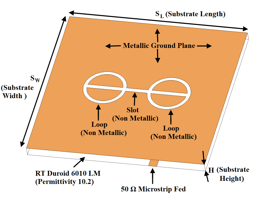
Figure 1: 3D view of Slot antenna loaded with two loops.

A slot antenna design with loops at both ends reduces resonance frequency and enhances miniaturization while maintaining performance. Quantum-Behaved Dynamic Particle Swarm Optimization (QDPSO) is used to optimize loop dimensions, ensuring improved performance and compactness. This data-driven approach combines computational optimization with machine learning for efficient slot antenna design. A data set of 936 simulation results generated using ANSYS HFSS [43] serves as the foundation for training machine learning algorithms, including SVM [44], random forest [45], XGBoost [46], and Stacked Model [47] allowing precise resonance frequency predictions based on loop dimension variations. The method efficiently tackles miniaturization and frequency tuning, providing a scalable solution for advanced wireless systems in record time. The paper is organized as follows: Section II covers antenna miniaturization, Section III discusses quantum-behaved dynamic PSO, Section IV addresses dataset integration with ML, Section V analyzes frequency prediction, Section VI highlights design automation, and Section VII summarizes key findings.

II Antenna design With Miniaturization Technique

The slot antenna is a compact, low-profile radiating structure ideal for wireless applications in consumer electronics like smartphones, tablets, and laptops, supporting Wi-Fi, Bluetooth, and cellular communication. For efficient radiation, the slot length should be half a wavelength. Excitation through a voltage source creates zero voltage at the slot edges due to shorting posts, resulting in maximum voltage at the center, one-quarter wavelength from each edge. Loops at both ends maintain this central maximum voltage, preserving the radiation properties of antenna.The three-dimensional schematic of the proposed antenna design is shown in Fig. 1. Miniaturization can be conceptualized through two distinct approaches. Since the wavelength of an antenna is inversely related to the resonant frequency, one method involves reducing the physical dimensions of the antenna while maintaining a constant resonant frequency. Conversely, the alternative strategy focuses on preserving the physical size of the antenna while lowering the resonant frequency. This study employs the latter approach to achieve miniaturization.

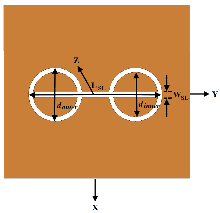
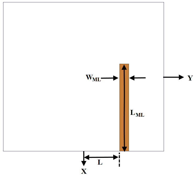
Figure 2: Top surface of slot antenna with loop.

Figure 3: Bottom surface of slot antenna with loop.

TABLE I: Parameter Specifications for Antenna Design

Category	Parameter	Value
Substrate Dimensions	Length	$L_{S}=100.00\,\text{mm}$
	Width	$W_{S}=100.00\,\text{mm}$
	Height	$H=2.54\,\text{mm}$
Slot Dimensions	Length	$L_{SL}=30.00\,\text{mm}$
	Width	$W_{SL}=1.20\,\text{mm}$
Microstrip Feed Line	Length	$L_{ML}=53.60\,\text{mm}$
	Trace Width	$W_{ML}=2.30\,\text{mm}$
	Stub Length	$L_{STB}=3.00\,\text{mm}$
	Offset	$L=9.00\,\text{mm}$ (y-axis)

Loops [5]–[7] are strategically positioned at both ends of the slot to enable antenna miniaturization, ensuring symmetrical geometry and consistent electromagnetic properties. In a half-wavelength slot, capacitive effects dominate below the resonance frequency, requiring compensation to achieve a lower resonance frequency.The loops positioned at either end of the slot exhibit an inductive nature, effectively compensating for the capacitive reactance present in the slot. This compensation creates the possibility of achieving a lower resonance frequency. The inner ($d_{\text{inner}}$) and outer ($d_{\text{outer}}$) diameters of the loop are critical in determining its width, a parameter that significantly influences the inductive effect. This inductive phenomenon is directly associated with the reduction in resonance frequency relative to the reference slot [7] frequency of 2.27 GHz. Therefore, the objective is to determine the optimal loop width to achieve the maximum reduction in resonance frequency. Fig. 2 illustrates the top surface of the antenna design to clarify the concept of integration between the slot and the loops. It is important to note that, for the slot and loops, the metallic portions are removed at the locations of the slot and loop on the ground plane. A $50\Omega$ microstrip feed line excites the slot antenna, positioned as a strip conductor on the bottom surface of the dielectric substrate, as shown in Fig. 3. The dimensions of the substrate, slot, and microstrip line are provided in Table I. The characteristics of the low-loss dielectric substrate RT Duroid 6010LM, with a relative permittivity $(\epsilon_{r})$ of 10.2, were selected for use in the simulations.

III Quantum-Behaved Dynamic Particle Swarm Optimization

Quantum-Behaved Dynamic Particle Swarm Optimization (QPSO) [19] combines quantum mechanics with traditional PSO to enhance search efficiency. Unlike classical PSO, which follows Newtonian dynamics, QPSO uses quantum-based probabilistic movement, improving exploration and exploitation while effectively avoiding local optima and achieving faster convergence toward global solutions. The OptiSLang, developed by ANSYS [43], serves as an advanced platform for process integration and robust design optimization across diverse engineering domains. For antenna design, OptiSLang employs a diverse array of cutting-edge optimization methodologies, including Particle Swarm Optimization [20], [21], [23], Surrogate-Based Optimization [28] and Genetic Algorithms [39], [40], [41]. After careful consideration, we opted QDPSO to refine the antenna configuration, based on the following compelling rationales: 1-Simplified Tuning: QDPSO requires only one control parameter, simplifying implementation compared to OptiSLang’s multi-parameter setup.2-Faster Convergence: The quantum-inspired search in QDPSO accelerates convergence, identifying optimal antenna designs more quickly than OptiSLang. 3-Enhanced Exploration: QDPSO’s quantum behavior improves solution space exploration, effectively avoiding local minima. 4- for Nonlinear Problems: QDPSO excels in optimizing complex, nonlinear antenna designs, outperforming some OptiSLang algorithms. 5-Tailored for Electromagnetics: QDPSO is designed for electromagnetic problems, making it more effective for antenna design than the general-purpose OptiSLang. 6-Lower Computational Cost: QDPSO’s efficient search and minimal parameters reduce computational demands compared to OptiSLang’s complex strategies.

III-A Antenna Optimization Process

In the context of slot antenna miniaturization using loops, the optimization focuses on the inner ($d_{\text{inner}}$) and outer ($d_{\text{outer}}$) diameters of the loop, while other dimensions and substrate properties, listed in Table I, remain unchanged. As discussed in Section II, the goal is to minimize the resonance frequency of the loop-loaded slot topology. The conventional process is difficult because it requires many trial-and-error simulations in ANSYS [43] to find the lowest resonance frequency, making the process very time-consuming. This optimization showcases the potential of automation to reduce engineering effort and shorten development cycles to a few hours. The flow chart of QDPSO is given in Fig. 4. The steps to get the best solutions are given as follows: 1- Initialization of Particles: Each particle $i$ is initialized with specific attributes. The position of the particle is determined by assigning the initial values for $d_{\text{inner}}$ and $d_{\text{outer}}$ randomly within their respective feasible ranges.

$$1.2\,\text{mm}<d_{\text{inner}}<d_{\text{outer}}\leq 12\,\text{mm}$$ (1)

$$d_{\text{outer}}-d_{\text{inner}}>0.8\,\text{mm}$$ (2)

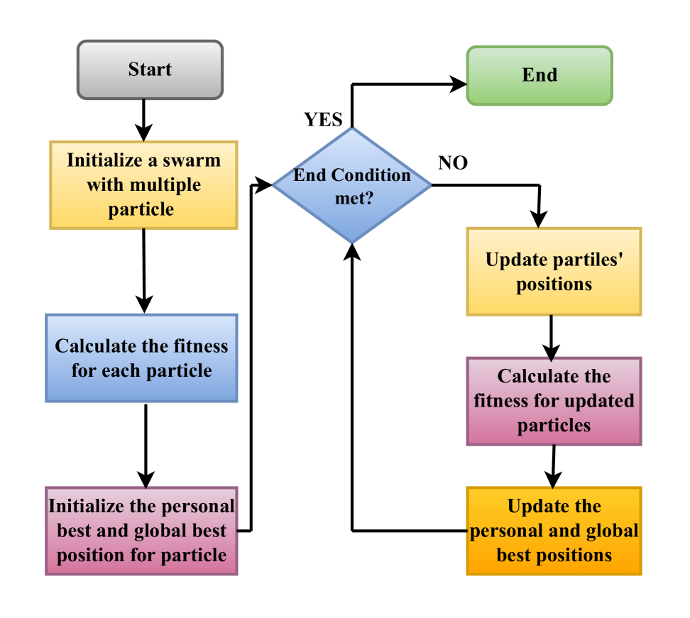
Figure 4: A Flowchart of the QDPSO

Specific geometric constraints are implemented to preserve the structural integrity and optimize the performance of the antenna. The inner diameter must exceed 1.20 mm, consistent with the slot width, to prevent merging with the slot, which could compromise structural stability. Similarly, the outer diameter is restricted to a maximum of 12.0 mm, as the slot length measures 30 mm and the combined length of the two loops is 24 mm. Surpassing this limit would induce overlap with the slot, increasing the overall antenna length and undermining the objective of resonance frequency reduction. Additionally, the difference between the outer and inner diameter must be no less than 0.80 mm to ensure feasibility for practical implementation. A smaller difference can cause fabrication issues and degrade antenna performance. Any particle position violating these limits is adjusted or resampled to stay within the defined parameter space, ensuring structural integrity and operational efficiency while meeting performance targets. Then, the initial position of each particle is set as its personal best $\mathbf{p}_{i}$. Among all particles, the one with the best fitness is chosen as the global best $\mathbf{g}$.

2- Evaluate Fitness: The fitness function evaluates how well each particle’s current position meets the target specifications. The closer $f_{r}$ is to the target frequency $f_{\text{target}}$, the higher the fitness. Additional constraints, such as return loss, and efficiency, may further influence the evaluation. 3- Update Global and Personal Bests: If a particle’s current position achieves a higher fitness than any previous position it held, this position becomes its new personal best $\mathbf{p}_{i}$. Among all particles, the position with the highest fitness is updated as the new global best $\mathbf{g}$. 4- Quantum-Inspired Position Update: Unlike classic PSO, QDPSO uses a quantum model for updating positions. Each particle’s new position is probabilistically determined to balance exploration and convergence is given by:

$$\mathbf{x}_{i}^{(t+1)}=\mathbf{p}_{i}+\beta\cdot|\mathbf{p}_{i}-\mathbf{g}|\cdot\ln\left(\frac{1}{u}\right)$$ (3)

where, the $x_{i}^{(t+1)}$ represents the new position of the particle $i$ at time $t+1$, the $p_{i}$ shows the personal best position of particle and $\beta$ is a contraction-expansion coefficient. The $g$ shows the global best position and variable $u$ is a random number uniformly distributed between $0$ and $1$ the term $|\mathbf{p}_{i}-\mathbf{g}|$ represents the Euclidean distance between the particle’s personal best and the global best, encouraging the particle to move closer to the globally optimal region.

This probabilistic update makes the particles ”quantum-behaved,” allowing them to potentially explore new areas within the search space instead of being confined by velocity-based movement. 5- Convergence Check: The algorithm iterates through steps 2-5 until it meets a convergence criterion, which could be: The process continues for a set number of iterations. It stops if there is minimal improvement in the global best fitness over a set number of iterations. The process can also stop if a fitness value reaches a defined threshold. 6- Final Solution: Once the algorithm converges, the global best position represents the optimal values for $d_{\text{inner}}$ and $d_{\text{outer}}$ that achieve the desired antenna performance. This solution balances the resonant frequency, return loss, bandwidth, and radiation efficiency.

Each particle in QDPSO navigates the search space using a probabilistic, quantum-inspired position update. Particles adapt their positions based on personal and global best experiences, balancing exploration and exploitation to optimize the antenna design effectively. The search process effectively converges to the optimal inner ($d_{\text{inner}}$) and outer ($d_{\text{outer}}$) diameters, enhancing antenna performance by minimizing the resonant frequency while adhering to specified design criteria.

III-B Fitness function definition and evaluation

The goal is to get the minimum resonant frequency $f_{r}$ of the antenna for a given target frequency $f_{\text{target}}$ that is 2.27 GHz. As our aim is to get a minimum $f_{r}$ value, we have to get the maximum absolute difference between $f_{r}$ and $f_{\text{target}}$. In equation 4, a novel fitness function is designed for that purpose.

$$\text{Minimize Fitness}=\frac{1}{1+|f_{r}-f_{\text{target}}|}$$ (4)

The fitness function is designed to reward solutions that maximize the difference between the resonant frequency ($f_{r}$) and the target frequency $f_{\text{target}}$. The term $|f_{r}-f_{\text{target}}|$ represents the absolute difference, and a larger absolute difference results in a lesser fitness value, encouraging the QDPSO algorithm to get a minimum $f_{r}$ value. Adding 1 to the denominator ensures that the fitness value remains finite and avoids division by zero when $|f_{r}-f_{\text{target}}|=0$, where the fitness value reaches its maximum of 1.
Here, $f_{r}$ (the resonant frequency) is a function of the antenna’s dimensions and the effective dielectric constant $\epsilon_{\text{eff}}$, and is calculated as:

$$f_{r}=\frac{c}{2\times(L_{SL}+d_{\text{outer}})\times\sqrt{\epsilon_{\text{eff}}}}$$ (5)

The effective dielectric constant $\epsilon_{\text{eff}}$ is approximated by:

$$\epsilon_{\text{eff}}=\frac{\epsilon_{r}+1}{2}+\frac{\epsilon_{r}-1}{2}\left(1+\frac{12h}{W}\right)^{-0.5}$$ (6)

TABLE II: Outer Diameter, Inner Diameter, Frequency, and Miniaturization Results

Outer Diameter	Inner Diameter	Frequency	Miniaturization
11.9787 mm	2.9498 mm	1.5912 GHz	29.90 %
11.6620 mm	7.0070 mm	1.5711 GHz	30.79 %
11.5439 mm	4.9963 mm	1.5411 GHz	32.11 %
11.9711 mm	3.2773 mm	1.5110 GHz	33.44 %
11.8729 mm	5.2052 mm	1.5110 GHz	33.44 %
11.1002 mm	2.2014 mm	1.4810 GHz	34.76 %
11.9187 mm	5.6182 mm	1.4409 GHz	36.52 %
11.8614 mm	6.2441 mm	1.4208 GHz	37.41 %

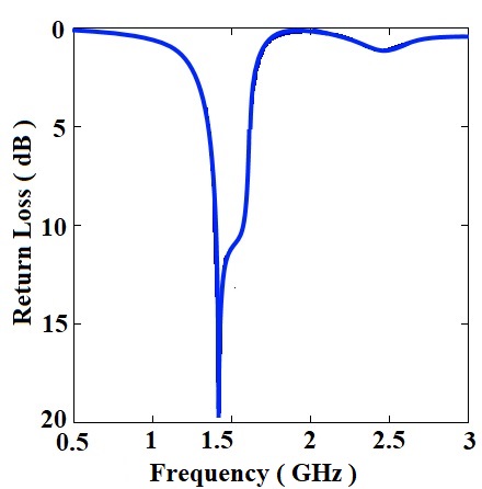
Figure 5: Return Loss for loop loaded slot antenna with Outer Diameter of 11.8614 mm and Inner Diameter of 6.2441 mm

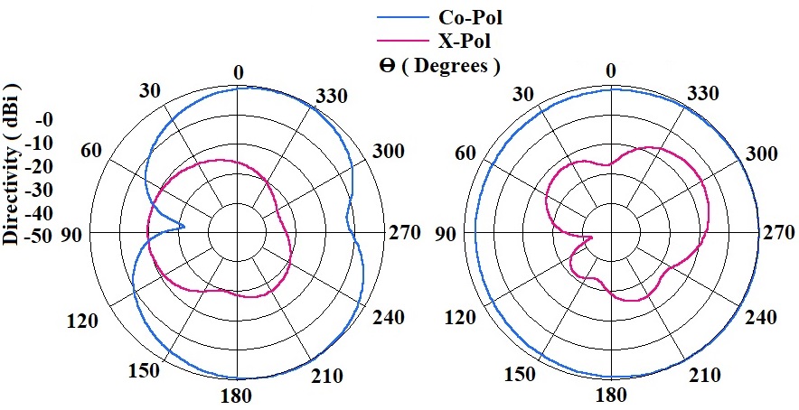
(a) E-Plane            (b) H-Plane

Figure 6: Radiation pattern at frequency 1.4208 GHz

III-C Optimization of slot antenna design using QDPSO and ANSYS

The QDPSO algorithm generates potential solutions for the inner $(d_{\text{inner}})$ and outer ($d_{\text{outer}}$) diameters of the loop, which are identical at both ends of the slot. These solutions are then implemented in ANSYS to determine the corresponding resonance frequencies. The results obtained from simulations using ANSYS, along with frequency reduction data, are analyzed in comparison to the reference slot’s frequency of 2.27 GHz, as detailed in Table II. This table delineates the responses for only 8 samples, although QDPSO is capable of generating a multitude of inner and outer diameter combinations, offering significant potential for optimal miniaturization. In comparison to Fig. 2 in the literature [7], the resonance frequency has been further reduced from 1.60 GHz to 1.4208 GHz, despite introducing less number of loops at either end of the slot.A comparative analysis proposes an alternative loop-loaded slot antenna design, improving miniaturization, time efficiency, and AI-CAD integration for rapid wireless devices development in a very short time. The return loss the loop loaded slot antenna, characterized by an outer diameter ($d_{\text{outer}}$) of 11.8614 mm and an inner diameter $(d_{\text{inner}})$ of 6.2441 mm, is depicted in Fig. 5, which demonstrates the maximum miniaturization achieved. The corresponding simulated ANSYS responses for the E-Plane and H-Plane are also shown in Fig. 6. Additionally, the QDPSO response achieved superior miniaturization compared to Fig. 8 in [5], demonstrating a 19.33% reduction for the slot antenna.

TABLE III: Constant Parameter Specifications for Data Set Creation

Parameter	Specification
Substrate Material Properties
Relative Permittivity ($\varepsilon_{r}$)	10.2 (Dielectric Constant)
Thickness	2.54 mm
Loss Tangent ($\tan\delta$)	0.0023 (Dielectric Losses)
Slot Design Parameters
Position (X, Y, Z)	(-0.6, -15, 0) Centrally on ground
Dimensions	Length: 30 mm, Width: 1.2 mm
Antenna Placement and Dimensions
Position (X, Y, Z)	(-50, -50, 0)
Dimensions	Length: 100 mm, Width: 100 mm
Loop Parameters
First Loop Position (X, Y, Z)	(0, -9, 0)
Second Loop Position (X, Y, Z)	(0, 9, 0)
Loop Placement	Positioned at either end of the slot
Microstrip Feed Line
Position (X, Y, Z)	(-3.6, 9, -2.54)
Dimensions	Length: 53.6 mm, Width: 2.3 mm
Microstrip feed Placement	Positioned at bottom surface

IV Data Sets And Machine Learning Algorithms

A primary challenge in applying machine learning to antenna design is the limited availability of datasets. While standard designs offer restricted data, bespoke antennas often necessitate the generation of proprietary datasets, which are crucial for developing precise and reliable models. In this study, the dataset for the proposed antenna was synthesized using ANSYS Electronics Desktop [43], comprising 936 data points. The design primarily emphasizes two critical parameters—the inner and outer diameters of the loop—which play a pivotal role in achieving optimal miniaturization, as depicted in Fig. 1. The dataset was generated by varying these two diameters and captures four key response variables: (1) resonance frequency, (2) return loss, (3) return loss depth, and (4) efficiency. All other dimensions were held constant, as detailed in Table III. Particular attention is given to the inner and outer diameters due to their significant influence on frequency reduction relative to the $\lambda$/2 slot resonance at 2.27 GHz. This focused investigation of the diameter dimensions is fundamental to enhancing both the miniaturization and overall performance of the antenna.

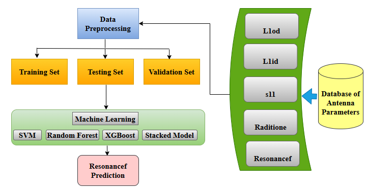
Figure 7: Steps to Predict the output

The subsequent analysis employs machine learning algorithms, such as SVM [44], Random Forest [45], XG Boost[46], and Stacked Model [47] to predict resonance frequency using 936 datasets.The algorithms used to predict the resonance frequency are detailed in the appendices A. The steps to calculate the predicted value of resonance frequency are given in Fig. 7.

V Results of Evaluation by Machine Learning framework

Fig. 8 illustrates the progression of a fitness function. The x-axis represents the number of iterations, while the y-axis shows the fitness value. The fitness value decreases as the absolute difference $|f_{r}-f_{\text{target}}|$ increases. In the initial phase (0–20 iterations), the fitness value improves rapidly, indicating that the algorithm effectively increases the difference $|f_{r}-f_{\text{target}}|$. This suggests that the initial solutions were far from the expected result, however, the algorithm quickly identifies promising regions of the solution space. The fitness value stabilizes in the plateau phase (after approximately 20 iterations), implying that the algorithm has maximized the difference to a nearly constant value.

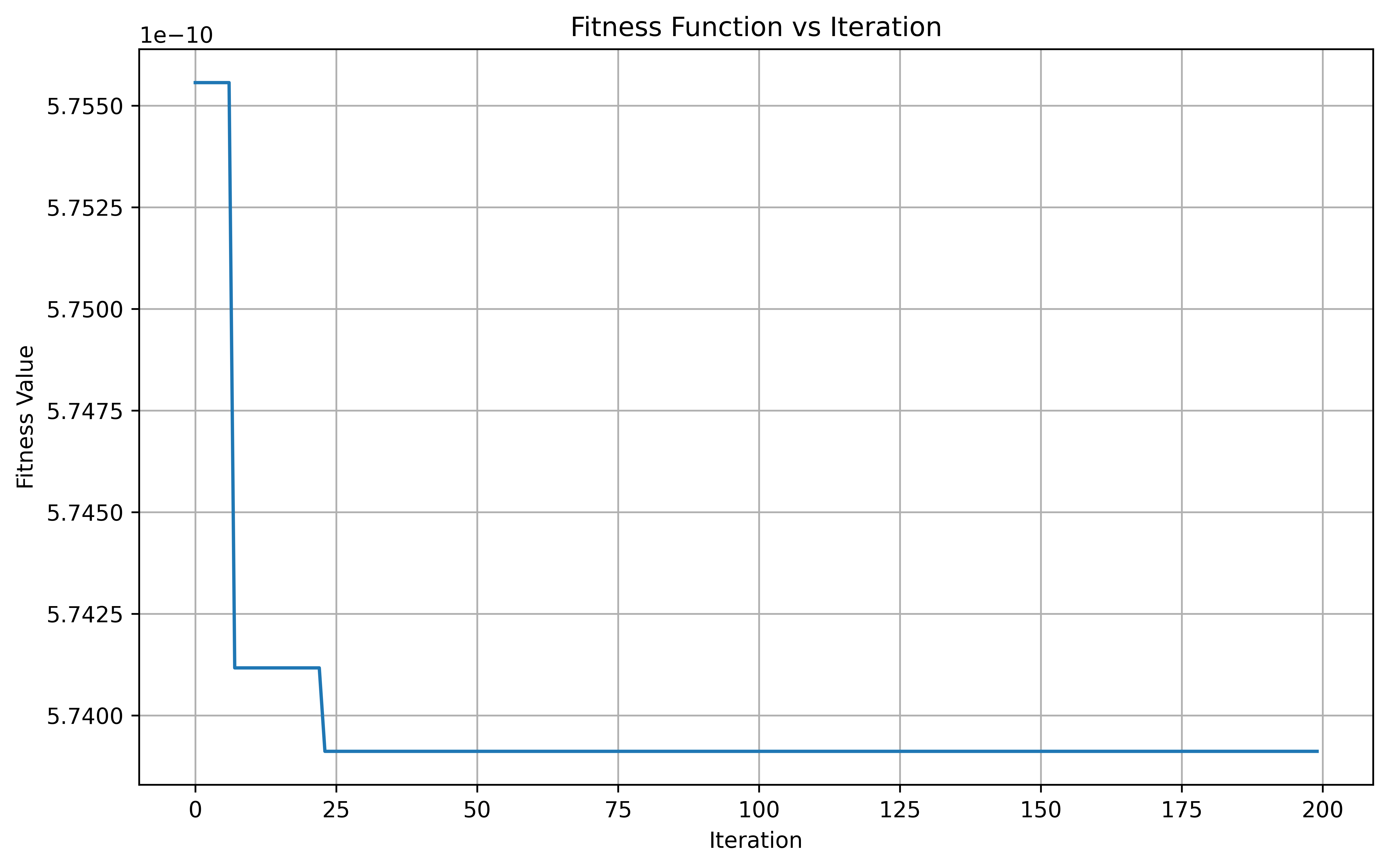
Figure 8: Fitness vs No. of Iterations

The data is split into 90% training data, 5% validation data, and 5% testing data. The large training dataset allows models to capture comprehensive patterns, while the validation set aids in fine-tuning hyperparameters and preventing overfitting. The base models are trained on the Training set, generating predictions for the Training, Testing, and Validation sets. These predictions are then combined to create stacked datasets for each split: $S_{train}$, $S_{test}$, and $S_{val}$. A detailed explanation of different machine learning models is given in Appendices A, B, and C. The performance of all models are evaluated using various metrics such as Mean Absolute Error ( MAE ), Mean Squared Error ( MSE ), Root Mean Squared Error( RMSE ), Coefficient of Determination ( R² ), Root Mean Squared Percentage Error ( RMSPE ), and Mean Absolute Percentage Error ( MAPE ) for the Training, Testing, and Validation sets. The use of MAE, MSE, RMSE, R², RMSPE, and MAPE is crucial in evaluating the performance of machine learning models as they provide various perspectives on accuracy, error distribution, and the model’s ability to generalize. These metrics help assess the deviation between predicted and actual values, ensuring that models are evaluated comprehensively across different error types. The detailed results are displayed in tables IV, V and VI.

TABLE IV: Performance Metrics of Models on Training Data

Model	MAE	MSE	RMSE	R²	RMSPE	MAPE
Random
Forest	0.0411	0.0046	0.0679	0.9410	4.7731	2.4355
SVM	0.1020	0.0264	0.1625	0.6616	11.3896	6.0921
XGBoost	0.0353	0.0026	0.0505	0.9673	3.2191	2.0333
Stacked
Model	0.0276	0.0014	0.0369	0.9825	2.1828	1.5492

TABLE V: Performance Metrics of Models on Testing Data

Model	MAE	MSE	RMSE	R²	RMSPE	MAPE
Random
Forest	0.1115	0.0236	0.1536	0.6938	9.2578	6.2138
SVM	0.0990	0.0190	0.1378	0.7537	8.0458	5.4768
XGBoost	0.1196	0.0288	0.1697	0.6263	10.1062	6.5767
Stacked
Model	0.1232	0.0303	0.1740	0.6075	10.4648	6.8221

TABLE VI: Performance Metrics of Models on Validation Data

Model	MAE	MSE	RMSE	R²	RMSPE	MAPE
Random
Forest	0.0933	0.0170	0.1303	0.6110	8.0510	5.3656
SVM	0.0858	0.0122	0.1106	0.7197	6.8617	4.9457
XGBoost	0.0931	0.0190	0.1380	0.5638	8.8563	5.4557
Stacked
Model	0.0953	0.0219	0.1480	0.4982	9.3922	5.5876

In the Fig.9 Based on the R² values on the training data, the stacked model demonstrates the best performance with an R² of 0.9825, indicating that it explains approximately 98.25% of the variance in the training data. This highlights the effectiveness of combining predictions from multiple models, as the stacked model leverages their strengths while minimizing individual weaknesses. XGBoost follows closely with an R² of 0.9673, showing its robustness and strong capability to model complex patterns. Random Forest, with an R² of 0.9410, performs well but is slightly less than XGBoost and the stacked model. In contrast, SVM exhibits the weakest performance on the training data with an R² of 0.6616, and its higher RMSE, RMSPE, and MAPE values indicate it struggles to capture the non-linear relationships in the data. Overall, on the training data, the stacked model and XGBoost emerge as the most effective approaches, with Random Forest being a reliable alternative.

Figure 9: Scatter plots of the different models during the Training phase

In Fig.10 on the validation data, the performance of the models based on R² values reveals distinct strengths and weaknesses. SVM demonstrates the best performance with an R² of 0.7197, indicating that it explains approximately 71.97% of the variance in the validation data. This highlights its capability to generalize well and effectively model the relationships in unseen data. Random Forest follows with an R² of 0.6110, showing moderate predictive ability, though it captures less variance compared to SVM. XGBoost, with an R² of 0.5638, performs slightly worse than Random Forest, suggesting its limited ability to handle the complexity of the validation data in this scenario. The stacked model, with the lowest R² of 0.4982, struggles the most on the validation data, explaining only 49.82% of the variance. This indicates that while the stacked model performed exceptionally well on the training data, it may be prone to overfitting, reducing its effectiveness on unseen data. Overall, SVM emerges as the most robust model on the validation data, followed by Random Forest and XGBoost, while the stacked model falls short in terms of generalization.

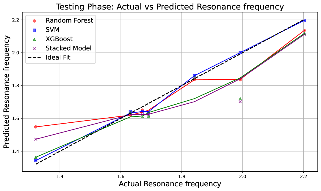
Figure 10: Scatter plots of the different models during the Testing phase

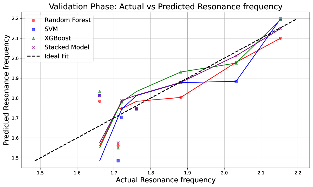
Figure 11: Scatter plots of the different models during the validation phase

In Fig.11 the SVM model outperforms the others with the highest R² value of 0.7197, explaining 71.97% of the variance in the actual resonance frequency values. This suggests that the SVM model provides the best fit, with the scatter plot showing tightly clustered points along the ideal fit line, indicating a strong correlation between predicted and actual values. The Random Forest model follows with an R² of 0.6110, explaining 61.1% of the variance, and its scatter plot shows moderate clustering around the diagonal line with some spread. XGBoost performs the worst with an R² of 0.5638, indicating that it explains only 56.38% of the variance, and the scatter plot for this model would show a greater spread of points, reflecting a weaker correlation between predictions and actual values. Surprisingly, the stacked model, which combines the predictions of the three models, performs the worst overall with an R² of 0.4982, indicating that it explains less than half of the variance. The scatter plot for the stacked model would show more dispersed points, reflecting its poorer fit compared to the individual models.

TABLE VII: Predicted and Actual Frequency

Outer Diameter	Inner Diameter	Frequency (GHz)
		Predicted	ANSYS
11.9787 mm	2.9498 mm	RF: 1.6290 SVM: 1.6135 XGB: 1.6327 SM: 1.6371	1.5912
11.6620 mm	7.0070 mm	RF: 1.6309 SVM: 1.6904 XGB: 1.6748 SM: 1.6457	1.5711
11.5439 mm	4.9963 mm	RF: 1.6209 SVM: 1.6687 XGB: 1.6194 SM: 1.6053	1.5411
11.9711 mm	3.2773 mm	RF: 1.5984 SVM: 1.5980 XGB: 1.5756 SM: 1.5815	1.5110
11.8729 mm	5.2052 mm	RF: 1.6500 SVM: 1.6664 XGB: 1.6701 SM: 1.6607	1.5110
11.1002 mm	2.2014 mm	RF: 1.6237 SVM: 1.5690 XGB: 1.6398 SM: 1.6531	1.4810
11.9187 mm	5.6182 mm	RF: 1.6966 SVM: 1.6441 XGB: 1.6880 SM: 1.7080	1.4409
11.8614 mm	6.2441 mm	RF: 1.5529 SVM: 1.6576 XGB: 1.6751 SM: 1.6109	1.4208

Table VII presents a comparative analysis of predicted resonance frequencies using four machine learning models, Random Forest (RF), Support Vector Machine (SVM), XGBoost (XGB), and Stacked Model (SM), against the actual frequencies obtained from ANSYS simulations. The predictions were evaluated for different combinations of outer and inner diameters of a circular structure. Across all cases, the predicted frequencies closely approximate the ANSYS results, with minor deviations observed. Notably, RF and SM generally exhibit smaller deviations from the actual frequencies, indicating robust predictive performance. However, SVM and XGB occasionally show larger discrepancies, particularly in cases with complex diameter configurations, such as for higher inner diameters. This analysis highlights the effectiveness of machine learning models, especially ensemble approaches like RF and XGB, in approximating high-fidelity simulations with a balance of accuracy and computational efficiency.

In this context, the SVM (Support Vector Machine) exhibited strong generalization, demonstrating its capability to handle non-linear relationships through kernel functions. XGBoost performed well, but its slight sensitivity to hyperparameters and potential overfitting on the validation data was noted. Random Forest delivered competitive results, with its ensemble learning ensuring stability but slightly underperforming compared to SVM due to less effective handling of complex non-linearities. The Stacked Model, combining predictions from base models, showed excellent training performance but slightly overfitted the data, as indicated by its lower validation performance. Thus, while training data optimizes model performance, validation ensures generalization and testing data verifies real-world applicability.

VI Rapid Wireless Device Production Through Automated Antenna Design

The rapid advancement of modern technology is driving a shift toward autonomous systems, including self-driving cars and automated drones. Similarly, Electronic Design Automation (EDA) [48] has transformed semiconductor development by automating complex design tasks, enabling the creation of highly sophisticated systems with billions of components. This highlights the need for similar automation in wireless consumer electronics, particularly in antenna design, to enhance efficiency and performance. An advanced automated antenna design system can be developed to allow users to specify performance requirements, upon which the system autonomously generates optimized design parameters along with precise fabrication instructions. In this study, the QDPSO optimization algorithm efficiently determined a representative set of loop dimensions within 11.53 seconds. Thereafter, the machine learning model predicted the corresponding resonance frequency in 0.75 seconds. The comprehensive design validation, performed in ANSYS and informed by the outputs of both the QDPSO and machine learning model, required 12 minutes 13.16 seconds prior to the commencement of antenna fabrication.The complete design finalization process required approximately 12.42 minutes, in contrast to the Parallel Surrogate-Assisted Differential Evolution Algorithm ( PSADEA ) [49], which demanded nearly 50 hours to achieve a comparable level of antenna design optimization.The work was performed on DESKTOP-8AAIDPT, equipped with an Intel Core i5-8500 (6 cores, 3.00 GHz), 16 GB RAM, and 64-bit Windows 10 Pro (Version 22H2) on an x64-based system.These prototypes enable rapid deployment in consumer and industrial applications, accelerating market entry. Conversely, in the absence of dimension predictions from QDPSO and frequency estimations from the ML model, the ANSYS design process becomes dependent on trial-and-error, resulting in an inherently unpredictable timeframe. While optimal results may occasionally be achieved quickly, the process often extends beyond a month, with experts typically requiring at least seven days, depending on design complexity. It can be claimed that automation in RF and microwave design boosts efficiency, accuracy, and integration, streamlining processes for faster, reliable production.

VII Conclusion

This research introduces an advanced framework for antenna miniaturization by combining Quantum-Behaved Dynamic Particle Swarm Optimization (QDPSO) and Machine Learning (ML) techniques. The approach addresses challenges in automated wireless system design by optimizing loop dimensions through QDPSO, achieving a 12.7 percent reduction in resonance frequency (1.4208 GHz vs. conventional 1.60 GHz) with optimization completed in 11.53 seconds. ML models trained on 936 ANSYS HFSS simulations predict resonance frequencies in 0.75 seconds, with the stacked ensemble model showing high training accuracy (R² = 0.9825) and SVM excelling in validation generalization (R² = 0.7197). The entire design cycle—optimization, prediction, and validation—is executed in 12.42 minutes on standard hardware, representing a 240× speed improvement over the PSADEA benchmark (50 hours) and eliminating traditional trial-and-error methods that often span over a week. This efficiency enables rapid deployment of compact antennas for IoT, 5G, and industrial applications while maintaining performance metrics like bandwidth and gain. Future directions include integrating multi-physics simulations for holistic validation, developing cloud-based AI platforms for automated geometry generation, incorporating sustainable materials, and addressing multi-band or massive MIMO requirements using metamaterials and phased array optimizations. By bridging AI-driven optimization with CAD validation, the framework establishes a scalable blueprint for next-generation RF systems, reducing engineering workloads and accelerating prototype development. Its adaptability to diverse frequencies and form factors positions it as a critical tool for autonomous drones and smart city infrastructure, enhancing both design agility and technological innovation.

Khan Masood Parvez (Student Member, IEEE)was born in Birbhum, India, in 1993. He received his B.E., M.E., and Ph.D. degrees in Electronics and Communication Engineering from Aliah University, Kolkata, India, in 2015, 2017, and 2025, respectively. His current research interests include slot antennas, antenna miniaturization, cross-polarization improvement, electrically small antennas, and machine learning.

Sk Md Abidar Rahaman received the B.Tech, M.Tech, and Ph.D degrees in Computer Science and Engineering from Aliah University in the years 2013, 2015, and 2025 respectively. His research interests include artificial intelligence, machine learning, and related applications. Dr. Rahaman has published several papers in reputable conferences, book chapters, and journals. He is currently working as a faculty member of Tarakeswar Degree College, affiliated with the University of Burdwan, in the department of computer science.

Ali Shiri Sichani (Member, IEEE) received the Ph.D. degree in electrical engineering from the University of South Florida, Tampa, FL, USA, in 2021.He is currently an Assistant Teaching Professor with the Electrical Engineering and Computer Science Department, University of Missouri, Columbia, MO, USA. His research interests include neuromorphic computing and VLSI, as well as hardware design for AI applications.

References

- [1] S. Silver, Microwave Antenna Theory and Design, New York, NY, USA:McGraw-Hill, pp. 296-298, 1946.
- [2] K. Fujimoto, H. Morishita, Modern Small Antennas. Cambridge, U.K.:Cambridge Univ. Press, 2013.
- [3] K. Sarabandi and R. Azadegan, “Design of an efficient miniaturized UHF planar antenna,” IEEE Trans. Antennas Propag., vol. 51, no. 6, pp. 1270-1276, June 2003.
- [4] R. Azadegan and K. Sarabandi, “A novel approach for miniaturization of slot antennas”, IEEE Trans. Antennas Propag., vol. 51, no. 3, pp. 421-429, Mar. 2003.
- [5] B. Ghosh, Sk. M. Haque, D. Mitra and S. Ghosh, “A loop loading technique for the miniaturization of non-planar and planar antennas”, IEEE Trans. Antennas Propag., vol. 58, no. 6, pp. 2116-2121, Jun. 2010.
- [6] B. Ghosh, Sk. M. Haque and D. Mitra, “Miniaturization of slot antennas using slit and strip loading”, IEEE Trans. Antennas Propag., vol. 59, no. 10, pp. 3922-3927, Oct. 2011.
- [7] SK. M. Haque and K. M. Parvez, “Slot Antenna Miniaturization Using Slit, Strip, and Loop Loading Techniques,” IEEE Trans. Antennas Propag., vol. 65, no. 5, pp. 2215-2221, May 2017.
- [8] B. Zheng, N. Li, X. Li, X. Rao and Y. Shan, “Miniaturized Wideband CP Antenna Using Hybrid Embedded Metasurface Structure,” IEEE Access, vol. 10, pp. 120056-120062, 2022.
- [9] L. Wang, X. -X. Yang, T. Lou and S. Gao, “A Miniaturized Differentially Fed Patch Antenna Based on Capacitive Slots,” IEEE Antennas Wirel. Propag. Lett., vol. 21, no. 7, pp. 1472-1476, July 2022.
- [10] Y. Li and J. Chen, “Design of Miniaturized High Gain Bow-Tie Antenna,” IEEE Trans. Antennas Propag., vol. 70, no. 1, pp. 738-743, Jan. 2022.
- [11] P. B. Samal, S. J. Chen and C. Fumeaux, “3-D-Corrugated Ground Structure: A Microstrip Antenna Miniaturization Technique,” IEEE Trans. Antennas Propag., vol. 72, no. 5, pp. 4010-4022,May 2024.
- [12] X. Yang, I. Calisir, L. Chen, E. L. Bennett, J. Xiao and Y. Huang, “A Study of Wideband and Compact Slot Antennas Utilizing Special Dispersive Materials,” IEEE Open J. Antennas Propag ,vol. 5, no. 5, pp. 1414-1422, Oct. 2024.
- [13] Q. Zheng, W. Liu, Q. Zhao, L. Kong, Y. -H. Ren and X. -X. Yang, “Broadband RCS Reduction, Antenna Miniaturization, and Bandwidth Enhancement by Combining Reactive Impedance Surface and Polarization Conversion Metasurface,” IEEE Trans. Antennas Propag., vol. 72, no. 9, pp. 7395-7400, Sept. 2024.
- [14] R. Gao, H. Sun, R. Ren and H. Zhang, “Design of a Biomedical Antenna System for Wireless Communication of Ingestible Capsule Endoscope,” IEEE Antennas Wirel. Propag. Lett., vol. 23, no. 12, pp.4243-4247, Dec. 2024.
- [15] A. Iqbal, M. Al-Hasan, I. Ben Mabrouk and T. A. Denidni, “A Compact Self-Triplexing Antenna for Head Implants,” IEEE Trans. Antennas Propag., vol. 72, no. 11, pp. 8207-8214, Nov. 2024.
- [16] S. D. Campbell, R. P. Jenkins, P. J. O’Connor, and D. Werner, “The explosion of artificial intelligence in antennas and propagation: How deep learning is advancing our state of the art,” IEEE Antennas Propag. Mag., vol. 63, no. 3, pp. 16–27, Jun. 2021.
- [17] Y. O. Cha, A. A. Ihalage, and Y. Hao, “Antennas and propagation research from large-scale unstructured data with machine learning: A review and predictions,” IEEE Antennas Propag. Mag., vol. 65,no. 5, pp. 10–24, Oct. 2023.
- [18] J. Robinson and Y. Rahmat-Samii, “Particle swarm optimization in electromagnetics,” IEEE Trans. Antennas Propag., vol. 52, no. 2,pp. 397–407, Feb. 2004.
- [19] S. M. Mikki and A. A. Kishk, “Quantum Particle Swarm Optimization for Electromagnetics,” IEEE Trans. Antennas Propag., vol. 54, no. 10, pp. 2764-2775, Oct. 2006.
- [20] S. Ahad, S. Yang, S. U. Khan, S. A. Khan, and R. A. Khan, “A hybrid smart quantum particle swarm optimization for multimodal electromagnetic design problems,” IEEE Access, vol. 10, pp. 72339–72347, 2022.
- [21] H. Han, Y. Liu, Y. Hou, and J. Qiao, “Multi-modal multi-objective particle swarm optimization with self-adjusting strategy,” Information Sciences, vol. 629, pp. 580–598, 2023.
- [22] X. Jia and G. Lu, “A hybrid Taguchi binary particle swarm optimization for antenna designs,” IEEE Antennas Wireless Propag. Lett., vol. 18, no. 8, pp. 1581–1585, Aug. 2019.
- [23] Lukasz A. Greda, Andreas Winterstein, Daniel L. Lemes, Marcos V. T. Heckler, “Beamsteering and Beamshaping Using a Linear Antenna Array Based on Particle Swarm Optimization”, IEEE Access, vol.7, pp.141562-141573, 2019.
- [24] Q. Wu, W. Chen, C. Yu, H. Wang and W. Hong, “Machine-Learning-Assisted Optimization for Antenna Geometry Design,” IEEE Trans. Antennas Propag., vol. 72, no. 3, pp. 2083-2095, March 2024.
- [25] Q. Wu, W. Chen, C. Yu, H. Wang, and W. Hong, “Multilayer machine learning-assisted optimization-based robust design and its applications to antennas and array,” IEEE Trans. Antennas Propag., vol. 69, no. 9,pp. 6052–6057, Sep. 2021.
- [26] W. Chen, Q. Wu, C. Yu, H. Wang and W. Hong, “Multibranch Machine Learning-Assisted Optimization and Its Application to Antenna Design,” IEEE Trans. Antennas Propag., vol. 70, no. 7, pp. 4985-4996, July 2022.
- [27] J. S. Smith and M. E. Baginski, “Thin-wire antenna design using a novel branching scheme and genetic algorithm optimization,” IEEE Trans. Antennas Propag., vol. 67, no. 5, pp. 2934–2941, May 2019.
- [28] B. Liu et al., “An efficient method for complex antenna design based on a self adaptive surrogate model-assisted optimization technique,” IEEE Trans. Antennas Propag., vol. 69, no. 4, pp. 2302–2315, Apr. 2021.
- [29] J. Zhou et al., “A trust-region parallel Bayesian optimization method for simulation-driven antenna design,” IEEE Trans. Antennas Propag., vol. 69, no. 7, pp. 3966–3981, Jul. 2021.
- [30] Y. Liu et al., “An efficient method for antenna design based on a selfadaptive Bayesian neural network assisted global optimization technique,” IEEE Trans. Antennas Propag., vol. 70, no. 12, pp. 11375–11388, Dec.2022.
- [31] S. Koziel and A. Pietrenko-Dabrowska, “Tolerance optimization of antenna structures by means of response feature surrogates,” IEEE Trans. Antennas Propag., vol. 70, no. 11, pp. 10988–10997, Nov. 2022.
- [32] A. Pietrenko-Dabrowska and S. Koziel, “Generalized formulation of response features for reliable optimization of antenna input characteristics,” IEEE Trans. Antennas Propag., vol. 70, no. 5, pp. 3733–3748, May 2022.
- [33] Y. Sharma, H. H. Zhang, and H. Xin, “Machine learning techniques for optimizing design of double T-shaped monopole antenna,” IEEE Trans.Antennas Propag., vol. 68, no. 7, pp. 5658–5663, Jul. 2020.
- [34] Y. Sharma, X. Chen, J. Wu, Q. Zhou, H. H. Zhang, and H. Xin, “Machine learning methods-based modeling and optimization of 3-Dprinted dielectrics around monopole antenna,” IEEE Trans. Antennas Propag., vol. 70, no. 7, pp. 4997–5006, Jul. 2022.
- [35] T. Lin and Y. Zhu, “Beam forming design for large-scale antenna arrays using deep learning,” IEEE Wireless Commun. Lett., vol. 9, no. 1,pp. 103–107, Jan. 2020.
- [36] A. M. Montaser and K. R. Mahmoud, “Deep learning based antenna design and beam-steering capabilities for millimeter-wave applications,” IEEE Access, vol. 9, pp. 145583–145591, 2021.
- [37] Q. Wu, W. Chen, C. Yu, H. Wang, and W. Hong, “Multilayer machine learning-assisted optimization-based robust design and its applications to antennas and array,” IEEE Trans. Antennas Propag., vol. 69, no. 9,pp.6052–6057, Sep. 2021.
- [38] Q. Xu, S. Zeng, F. Zhao, R. Jiao, and C. Li, “On formulating and designing antenna arrays by evolutionary algorithms,” IEEE Trans.Antennas Propag., vol. 69, no. 2, pp. 1118–1129, Feb. 2021.
- [39] J. S. Smith and M. E. Baginski, “Thin-wire antenna design using a novel branching scheme and genetic algorithm optimization,” IEEE Trans. Antennas Propag., vol. 67, no. 5, pp. 2934–2941, May 2019.
- [40] N. Herscovici, M. F. Osorio and C. Peixeiro, ”Miniaturization of rectangular microstrip patches using genetic algorithms,” IEEE Antennas Wirel. Propag. Lett., vol. 1, pp. 94-97, 2002.
- [41] John, M. and M. J. Ammann, “Wideband printed monopole design using genetic algorithm,” IEEE Antennas Wirel. Propag. Lett., Vol. 6, 447–449, 2007.
- [42] D. Shi, C. Lian, K. Cui, Y. Chen, and X. Liu, “An intelligent antenna synthesis method based on machine learning,” IEEE Trans. Antennas Propag., vol. 70, no. 7, pp. 4965–4976, Jul. 2022.
- [43] ANSYS Corporation Ver 18.2 ,“ HFSS,” Pittsburgh, PA, 15317.
- [44] Keerthi SS, Shevade SK, Bhattacharyya C, Radha Krishna MK, “Improvements to platt’s SMO algorithm for SVM classifier design,” Neural Comput., 2001;13(3):637–49.
- [45] Breiman L. Random forests. Mach Learn. 2001;45(1):5–32.
- [46] Pedregosa F, Varoquaux G, Gramfort A, Michel V, Thirion B, Grisel O, Blondel M, Prettenhofer P, Weiss R, Dubourg V, et al. Scikit-learn: machine learning in python. J Mach Learn Res. 2011;12:2825–30.
- [47] D. H. Wolpert, “Stacked generalization,” Neural Networks, vol. 5, no. 2, pp. 241-259, 1992.
- [48] C. Mead and L. Conway, “Introduction to VLSI Systems,” IEEE Journal of Solid-State Circuits, vol. 15, no. 6, pp. 1068-1075, Dec. 1980.
- [49] I. M. Danjuma, M. O. Akinsolu, C. H. See, R. A. Abd-Alhameed, and B. Liu, ”Design and optimization of a slotted monopole antenna for ultra-wide band body centric imaging applications,” IEEE J. Electromagn., RF Microw. Med. Biol., vol. 4, no. 2, pp. 140–147, Jun. 2020.