Estimation of the number of principal components
in high-dimensional multivariate extremes

Abstract

For multivariate regularly random vectors of dimension $d$, the dependence structure of the extremes is modeled by the so-called angular measure. When the dimension $d$ is high, estimating the angular measure is challenging because of its complexity. In this paper, we use Principal Component Analysis (PCA) as a method for dimension reduction and estimate the number of significant principal components of the empirical covariance matrix of the angular measure under the assumption of a spiked covariance structure. Therefore, we develop Akaike Information Criteria ($\operatorname{AIC}$) and Bayesian Information Criteria ($\operatorname{BIC}$) to estimate the location of the spiked eigenvalue of the covariance matrix, reflecting the number of significant components, and explore these information criteria on consistency. On the one hand, we investigate the case where the dimension $d$ is fixed, and on the other hand, where the dimension $d$ converges to $\infty$ under different high-dimensional scenarios. When the dimension $d$ is fixed, we establish that the $\operatorname{AIC}$ is not consistent, whereas the $\operatorname{BIC}$ is weakly consistent. In the high-dimensional setting, with techniques from random matrix theory, we derive sufficient conditions for the $\operatorname{AIC}$ and the $\operatorname{BIC}$ to be consistent. Finally, the performance of the different $\operatorname{AIC}$ and $\operatorname{BIC}$ versions is compared in a simulation study and applied to high-dimensional precipitation data.

and

1 Introduction

In multivariate extreme value theory, extremes occur per se rarely so that the dimensionality of the data in fields such as finance, insurance, meteorology, hydrology, and, more broadly, environmental risk assessment often approaches or exceeds the number of extreme observations which is a big challenge in the statistical analysis of complex and high-dimensional data. Therefore, a standard approach from multivariate statistics is to apply a dimension reduction method to reduce the model complexity and circumvent the curse of dimensionality. A very nice overview of different methods for constructing sparsity in high-dimensional multivariate extremes is given in Engelke:Ivanovs, including Principle Component Analysis (PCA), spherical $k$-means, graphical models, or sparse regular variation, to mention a few.

In multivariate statistics, PCA is a widely used method for dimension reduction, data visualization, clustering and feature extraction ([muirhead:1982, anderson:2003]). In recent years, the literature on implementing PCA for high-dimensional and complex data of multivariate extremes to construct some sparsity in the data has grown rapidly ([chautru, DS:21, Sabourin_et_al_2024, CT:19, MR4582715, drees2025asymptoticbehaviorprincipalcomponent, wan2024characterizing]). A classical concept of multivariate extreme value theory is multivariate regular variation ([resnick:1987, resnick:2007, Falk:Buch]). A $d$-dimensional random vector $\boldsymbol{X}$ is multivariate regularly varying of index $\alpha>0$ if there exists a random vector $\boldsymbol{\Theta}$ on the unit sphere such that

$$\mathbb{P}\left(\frac{\lVert\boldsymbol{X}\rVert}{t}>r,\frac{\boldsymbol{X}}{\lVert\boldsymbol{X}\rVert}\in\cdot\Big{|}\,\lVert\boldsymbol{X}\rVert>t\right)\overset{\mathcal{D}}{\longrightarrow}r^{-\alpha}\mathbb{P}(\boldsymbol{\Theta}\in\cdot),\quad t\rightarrow\infty,$$

for all $r>0$. The dependence structure of the extremes of $\boldsymbol{X}$ is modeled in the spectral vector $\boldsymbol{\Theta}$ whose distribution is also called angular measure and its covariance matrix is denoted as $\boldsymbol{\Sigma}=\operatorname{Cov}(\boldsymbol{\Theta})$. drees2025asymptoticbehaviorprincipalcomponent and DS:21 set the mathematical framework for PCA for the empirical covariance estimator of $\boldsymbol{\Sigma}=\operatorname{Cov}(\boldsymbol{\Theta})$ by analyzing the squared reconstruction error, the excess risk and their asymptotic behavior. However, until now, the research on the number of significant principal components, the so-called dimensionality, in PCA for multivariate extremes, is limited. In DS:21, the dimension was estimated through the examination of empirical risk plots. An alternative approach is to analyze the scree plot, which is the plot of the empirical eigenvalues, in search of an ”elbow” as a cutoff point, indicating a minimal variation in the empirical eigenvalues after this point. But a big challenge in extreme value theory is the choice of the threshold $t$, which defines the extreme observations as the data whose norm is above $t$. Changing this threshold also changes the number of extreme observations and the estimates of the empirical eigenvalues. Thus, a change of the threshold results in a different scree plot and possibly also in a different elbow. Given the ambiguity and uncertainty of both methods, as well as the need for case-by-case evaluation, a mathematically based approach is necessary. One of the few works that developed a statistical method for estimating the dimensionality is given in drees2025asymptoticbehaviorprincipalcomponent, whose method is based on asymptotic results for the reconstruction error of the projections and is a kind of testing problem with the disadvantage that it depends on different tuning parameters.

In this paper, we propose information criteria to estimate the number of significant principal components in multivariate extremes modeled through the covariance matrix $\boldsymbol{\Sigma}$ of $\boldsymbol{\Theta}$. Therefore, we combine an approach of Bai:Choi:Fujikoshi:2018 and jiang:2023 from high-dimensional statistics with methods from extreme value theory ([resnick:1987, resnick:2007, HF:2006]) and random matrix theory ([Bai:Silverstein:2010]). We assume a spiked covariance model for the covariance matrix $\boldsymbol{\Sigma}$ which goes back to johnstone:2001 and is widely used in high-dimensional statistics ([Bai:Choi:Fujikoshi:2018, Bai:Yao:2012, fujikoshi:sakurai:2016, jiang:2023, johnstone:2018]) with applications in various fields, e.g., speech recognition, wireless communication and statistical learning as mentioned in Paul:2007.

Spiked Covariance Model:   The eigenvalues $\lambda_{1},\ldots,\lambda_{d}$ of $\boldsymbol{\Sigma}$ satisfy

$$\lambda_{1}\geq\lambda_{2}\geq\cdots\geq\lambda_{p^{*}}>\lambda_{{p^{*}}+1}=\cdots=\lambda_{d-1}\eqqcolon\lambda>0.$$ (1.1)

The smallest eigenvalue $\lambda_{d}$ is not considered to avoid numerical instability as it can be equal to $0$, if, for example, $\boldsymbol{\Theta}$ is concentrated on the subspace of the unit sphere with non-negative values. The main objective of this article is to develop an estimator $\widehat{p}_{n}$ for the unknown dimensionality parameter $p^{*}$ of significant eigenvalues of $\boldsymbol{\Sigma}$ through information criteria. When $d$ is relatively large compared to $\widehat{p}_{n}$, the data are projected on the $\widehat{p}_{n}$-dimensional subspace spanned by the empirical eigenvectors of the largest $\widehat{p}_{n}$ empirical eigenvalues $\widehat{\lambda}_{n,1},\ldots,\widehat{\lambda}_{n,\widehat{p}_{n}}$. This lower-dimensional representation allows for more extensive and in-depth analyses of the dependence structure in the extremes.

The estimation of the dimensionality $p^{*}$ in PCA is explored in this paper using two information criteria: the Akaike Information Criterion ($\operatorname{AIC}$) and the Bayesian Information Criterion ($\operatorname{BIC}$). Similar information criteria were investigated in fujikoshi:sakurai:2016 for Gaussian random vectors in a large-sample asymptotic framework and in Bai:Choi:Fujikoshi:2018 for general data in the high-dimensional case. Both criteria are motivated by a Gaussian likelihood function, although our underlying model for $\boldsymbol{\Theta}$ is not Gaussian. Since in a Gaussian spiked covariance model with $k_{n}$ observations, the log likelihood function can be written as a functional of the empirical eigenvalues in the form

$$k_{n}\sum_{i=1}^{p^{*}}\log(\widehat{\lambda}_{n,i})+k_{n}(d-p^{*})\log\Big{(}\sum_{j=p^{*}}^{d}\frac{\widehat{\lambda}_{n,j}}{d_{n}-p^{*}}\Big{)}+k_{n}\log\Big{(}\frac{k_{n}-1}{k_{n}}\Big{)}^{d}+k_{n}d(\log(2\pi)+1),$$

both the AIC and BIC are defined as functionals of the empirical eigenvalues $\widehat{\lambda}_{n,1},\ldots,\widehat{\lambda}_{n,d}$.

The main goal of this paper is to derive necessary and sufficient conditions for our AIC and BIC to be consistent. Therefore, we require methods from random matrix theory to derive the asymptotic properties of the empirical eigenvalues, which are the basic components of the AIC and BIC. For this purpose, we differentiate between two cases when $n$ observations are available and of these $k_{n}$ are extreme. The first is the classic large sample size and fixed-dimension case, where $n\to\infty$ and the dimension $d$ is fixed. As is typical for such information criteria, we find that the BIC is consistent, whereas the AIC is, in general, not consistent. In the second case, we assume that $d=d_{n}$ also depends on $n$ and $d_{n}/k_{n}\rightarrow c>0$ as $n\to\infty$. In this case, the empirical eigenvalues are not consistent estimators for the eigenvalues anymore. For high-dimensional i.i.d. data with finite fourth moments, it is well-known that the empirical spectral distribution function converges to the Marčenko-Pastur law ([marchenko:pastur:1967]), which describes the bulk distribution of the empirical eigenvalues. The spiked covariance model, introduced by johnstone:2001, extends the Marčenko-Pastur framework by adding a small number of spiked eigenvalues corresponding to relevant dimensions for the PCA. In the context of this paper, we derive as well the asymptotic properties of the empirical eigenvalues of $\boldsymbol{\Sigma}$ with the Marčenko-Pastur distribution in the limit and use it for the investigation of the consistency of our information criteria. To the best of our knowledge, this paper is the first paper to develop consistent information criteria for the dimensionality $p^{*}$ of the PCA in high-dimensional multivariate extremes. The only other information criteria of meyer_muscle23 and butsch2024fasen use the concept of sparse regular variation to construct sparsity in the data, in contrast to PCA.

Structure of the paper

This paper is organized as follows. In Section 2, we properly define the empirical eigenvalues $\widehat{\lambda}_{n,1},\ldots,\widehat{\lambda}_{n,d}$ of $\boldsymbol{\Sigma}$, which are the main components in the definition of the information criteria. In addition, we explore the asymptotic properties of the empirical eigenvalues, where in the high-dimensional case we restrict our study to a parametric family of distributions, the so-called directional model. The subject of Section 3 are the $\operatorname{AIC}$ and the $\operatorname{BIC}$ for estimating the location $p^{*}$ of the spiked eigenvalue in the fixed-dimensional case, where Section 4 explores the high-dimensional case when $d_{n}/k_{n}\rightarrow c>0$ as $n\to\infty$. We will examine the case $0<c<1$ and $c>1$ separately in Section 4.1 and Section 4.2, respectively. In both cases, we derive sufficient criteria for the $\operatorname{AIC}$ and the $\operatorname{BIC}$ to be weakly consistent. In a simulation study in Section 5, we compare the different information criteria and apply them to precipitation data in Section 6. Finally, we state a conclusion in Section 7. The proofs for the results presented in this paper are provided in the Appendix.

Notation

Throughout the paper, we use the following notation and assume that all random variables are defined on the same probability space $(\Omega,\mathcal{F},\mathbb{P})$. First of all, $\|\boldsymbol{x}\|$ is the Euclidean norm for $\boldsymbol{x}\in\mathbb{R}^{d}$ and $\|{\boldsymbol{A}}\|$ is the spectral norm for matrices ${\boldsymbol{A}}\in\mathbb{R}^{d\times d}$. The matrix $\boldsymbol{I}_{d}\in\mathbb{R}^{d\times d}$ is the identity matrix, $\boldsymbol{e}_{i}$ is the $i$-th unit vector with $1$ at the $i$-th entry and $0$ else, $\boldsymbol{0}_{d}\coloneqq(0,\ldots,0)^{\top}\in\mathbb{R}^{d}$ is the zero vector and $\boldsymbol{1}_{d}:=(1,\ldots,1)^{\top}\in\mathbb{R}^{d}$ is the vector containing only $1$. For a vector $\boldsymbol{x}\in\mathbb{R}^{d}$ we write $\operatorname{diag}(\boldsymbol{x})\in\mathbb{R}^{d\times d}$ for a diagonal matrix with the components of $\boldsymbol{x}$ on the diagonal and for ${\boldsymbol{A}}=(\boldsymbol{a}^{(1)},\ldots,\boldsymbol{a}^{(d)})\in\mathbb{R}^{d\times d}$ the operator $\operatorname{vec}({\boldsymbol{A}})\in\mathbb{R}^{d^{2}}$ stacks the columns of ${\boldsymbol{A}}$ in a vector such that $\operatorname{vec}({\boldsymbol{A}})=({\boldsymbol{a}^{(1)}}^{\top},\ldots,{\boldsymbol{a}^{(d)}}^{\top})^{\top}$ and $\lambda_{i}({\boldsymbol{A}})$ denotes the $i$-th largest eigenvalue of ${\boldsymbol{A}}$. If $\boldsymbol{B}\in\mathbb{R}^{d\times d}$ and ${\boldsymbol{A}}=\boldsymbol{B}^{2}\in\mathbb{R}^{d\times d}$ then ${\boldsymbol{A}}^{1/2}\coloneqq\boldsymbol{B}$ denotes the square root of a matrix. A sequence of matrices ${\boldsymbol{A}}_{1},{\boldsymbol{A}}_{2},\ldots\in\mathbb{R}^{d\times d}$ with fixed dimension $d$ is denoted by $({\boldsymbol{A}}_{n})_{n\in\mathbb{N}}$ and if the dimensions $d=d_{n}$ depends on $n$, we write $({\boldsymbol{A}}^{(n)})_{n\in\mathbb{N}}$, where ${\boldsymbol{A}}^{(n)}\in\mathbb{R}^{d_{n}\times d_{n}}$. For a univariate distribution function $F$ the function $F^{\leftarrow}:(0,1)\rightarrow\mathbb{R}$ with $p\mapsto\inf\{x\in\mathbb{R}:F(x)\geq p\}$ is the generalized inverse of $F$. By $\delta_{\boldsymbol{x}}$ we denote the Dirac measure in $\boldsymbol{x}\in\mathbb{R}^{d}$. Finally, $\overset{\mathcal{D}}{\longrightarrow}$ is the notation for convergence in distribution, $\overset{\mathbb{P}}{\longrightarrow}$ is the notation for convergence in probability and $\overset{\mathbb{P}\text{-a.s.}}{\longrightarrow}$ is the notation for almost sure convergence.

2 Asymptotic behavior of the empirical eigenvalues of $\boldsymbol{\Sigma}$

The information criteria AIC and BIC of this paper are defined by the empirical eigenvalues $\widehat{\lambda}_{n,1},\ldots,\widehat{\lambda}_{n,d}$ of $\boldsymbol{\Sigma}$. Therefore, in the first step, in Section 2.1, we define and explore the empirical eigenvalues and their asymptotic properties in the fixed-dimensional case, and then, in Section 2.2, in the high-dimensional case. With the knowledge of the asymptotic behavior of the empirical eigenvalues, we will be able to derive the asymptotic behavior of the AIC and the BIC in Section 3 and Section 4. The proofs of this section are moved to Appendix A.

2.1 Fixed-dimensional case

In the case where the dimension $d$ is fixed, we consider the following model.

Model A.

1. Let $\boldsymbol{X},\boldsymbol{X}_{1},\boldsymbol{X}_{2},\ldots$ be a sequence of i.i.d. regularly varying random vectors with tail index $\alpha>0$ and spectral vector $\boldsymbol{\Theta}$.

2. The eigenvalues $\lambda_{1},\ldots,\lambda_{d}$ of $\boldsymbol{\Sigma}=\operatorname{Cov}(\Theta)$ satisfy

   $$\lambda_{1}\geq\lambda_{2}\geq\cdots\geq\lambda_{p^{*}}>\lambda_{{p^{*}}+1}=\cdots=\lambda_{d-1}\eqqcolon\lambda>0.$$

3. Let $(k_{n})_{n\in\mathbb{N}}$ be a sequence in $\mathbb{N}$ with $k_{n}\rightarrow\infty$ and $k_{n}/n\rightarrow 0$ for $n\rightarrow\infty$.

4. Suppose $u_{n}$ is a sequence such that for $n\to\infty$, $n\mathbb{P}(\|\boldsymbol{X}\|>u_{n})/k_{n}\to 1$ and

   $$\sup_{x\in[\frac{1}{1+\tau},1+\tau]}\sqrt{k_{n}}\left\|\frac{n}{k_{n}}\mathbb{E}\left[\begin{pmatrix}\frac{\operatorname{vec}(\boldsymbol{X}\boldsymbol{X}^{\top})}{\lVert\boldsymbol{X}\rVert^{2}}\\ 1\end{pmatrix}\mathbbm{1}\{x\lVert\boldsymbol{X}\rVert>u_{n}\}\right]-x^{\alpha}\begin{pmatrix}\operatorname{vec}(\mathbb{E}[\boldsymbol{\Theta}\boldsymbol{\Theta}^{\top}])\\ 1\end{pmatrix}\right\|\rightarrow 0,$$

   as $n\to\infty$.

The last assumption (A4) is a technical assumption that we require for some proofs (cf. Remark 2.2). Under these model assumptions, the empirical estimator for $\boldsymbol{\Theta}$ is defined as

$$\widehat{\boldsymbol{\Theta}}_{n}\coloneqq\frac{1}{k_{n}}\sum_{i=1}^{n}\frac{\boldsymbol{X}_{i}}{\lVert\boldsymbol{X}_{i}\rVert}\mathbbm{1}\{\lVert\boldsymbol{X}_{i}\rVert>\|\boldsymbol{X}_{(k_{n}+1,n)}\|\},$$

and hence, the empirical covariance matrix $\widehat{\boldsymbol{\Sigma}}_{n}$ of $\boldsymbol{\Sigma}$ is

$$\widehat{\boldsymbol{\Sigma}}_{n} \coloneqq\frac{1}{k_{n}}\sum_{j=1}^{n}\left(\frac{\boldsymbol{X}_{j}}{\|\boldsymbol{X}_{j}\|}-\widehat{\boldsymbol{\Theta}}_{n}\right)\left(\frac{\boldsymbol{X}_{j}}{\|\boldsymbol{X}_{j}\|}-\widehat{\boldsymbol{\Theta}}_{n}\right)^{\top}\mathbbm{1}\{\|\boldsymbol{X}_{j}\|>\|\boldsymbol{X}_{(k_{n}+1,n)}\|\}$$ (2.1)

with eigenvalues $\widehat{\lambda}_{n,1},\ldots,\widehat{\lambda}_{n,d}$ where $n\in\mathbb{N}$ is the number of observations and $\boldsymbol{X}_{(k_{n}+1,n)}$ denotes the observation with the $(k_{n}+1)$-th largest norm. Both the AIC and the BIC information criteria for the estimation of $p^{*}$ will be defined by the empirical eigenvalues $\widehat{\lambda}_{n,1},\ldots,\widehat{\lambda}_{n,d}$. Therefore, it is important to know the asymptotic behavior. We start to derive the asymptotic behavior of the empirical covariance matrix $\widehat{\boldsymbol{\Sigma}}_{n}$ in the next proposition and use this to derive the asymptotic behavior of the empirical eigenvalues.

Proposition 2.1.

Let Model A be given. Then as $n\to\infty$,

$$\sqrt{k_{n}}\bigl{(}\widehat{\boldsymbol{\Sigma}}_{n}-\boldsymbol{\Sigma}\bigr{)}\overset{\mathcal{D}}{\longrightarrow}\boldsymbol{S},$$

where $\operatorname{vec}(\boldsymbol{S})$ follows a centered normal distribution with covariance matrix

$$\operatorname{Cov}\bigl{(}\operatorname{vec}((\boldsymbol{\Theta}-\mathbb{E}[\boldsymbol{\Theta}])(\boldsymbol{\Theta}-\mathbb{E}[\boldsymbol{\Theta}])^{\top})\bigr{)}.$$

Remark 2.2.

In the bivariate case and for $h:\mathbb{R}^{2}\mapsto\mathbb{R}$ defined as $h(x,y)=xy$, the asymptotic distribution of

$$\frac{1}{k_{n}}\sum_{i=1}^{n}h\left(\frac{\boldsymbol{X}_{i}}{\lVert\boldsymbol{X}_{i}\rVert}\right)\mathbbm{1}\{\lVert\boldsymbol{X}_{i}\rVert>\|\boldsymbol{X}_{(k_{n}+1,n)}\|\}$$

was derived in Larsson:Resnick:2012. The techniques of the proof can be generalized and applied to $\operatorname{vec}(\widehat{\boldsymbol{\Sigma}}_{n})$ with the technical assumption (A4), and therefore, the proof of Proposition 2.1 is omitted. Note that if $\|\boldsymbol{\theta}\|=1$ for $\boldsymbol{\theta}\in\mathbb{R}^{d}$ then $\|\operatorname{vec}(\boldsymbol{\theta}\boldsymbol{\theta}^{\top})\|=1$ and higher moments of $\boldsymbol{\Theta}$ exist, since $\boldsymbol{\Theta}$ is bounded. A complementary result on the asymptotic behavior of the empirical covariance matrix is also given in the recent publication drees2025asymptoticbehaviorprincipalcomponent.

Now, we are able to present the asymptotic distribution of the empirical eigenvalues.

Theorem 2.3.

Let Model A be given.

1. Then as $n\to\infty$,

   $$(\widehat{\lambda}_{n,1},\ldots,\widehat{\lambda}_{n,d-1})=(\lambda_{1},\ldots,\lambda_{d-1})+O_{\mathbb{P}}(1/\sqrt{k_{n}}),$$

2. and

   $$\sqrt{k_{n}}\big{(}(\widehat{\lambda}_{n,p^{*}+1},\ldots,\widehat{\lambda}_{n,d-1})-\lambda\mathbf{1}_{d-p^{*}-1}\big{)}\overset{\mathcal{D}}{\longrightarrow}\boldsymbol{M},$$

   where the entries of the random vector $\boldsymbol{M}\in\mathbb{R}^{d-p^{*}-1}$ are the $(d-p^{*}-1)$ largest eigenvalues of $\boldsymbol{P}_{\lambda}\boldsymbol{S}\boldsymbol{P}_{\lambda}$ in decreasing order, $\boldsymbol{S}$ is defined as in Proposition 2.1 and $\boldsymbol{P}_{\lambda}\in\mathbb{R}^{d\times d}$ is the orthogonal projection onto the space spanned by the eigenvectors with respect to the eigenvalue $\lambda$ of $\boldsymbol{\Sigma}$.

2.2 Directional model in the high-dimensional case

In the high-dimensional setting, where $d=d_{n}$ depends on $n$ and $d_{n}\rightarrow\infty$ as $n\to\infty$, we restrict our studies to a parametric family of distributions, the so-called directional model. A directional model has the advantage that the underlying random vectors have an independent radial and directional component, but still the covariance matrix $\boldsymbol{\Sigma}^{(n)}$ has a spiked structure. The explicit definition of a directional model is the following.

Directional Model (D):   Suppose for any $n\in\mathbb{N}$ that

$${{\boldsymbol{\Gamma}}^{(n)}}\coloneqq\begin{pmatrix}\boldsymbol{\Gamma}_{n}&\boldsymbol{0}_{p^{*}\times d_{n}}\\ \boldsymbol{0}_{d_{n}\times p^{*}}&\boldsymbol{I}_{d_{n}-p^{*}}\end{pmatrix}\in\mathbb{R}^{d_{n}\times d_{n}},$$ (2.2)

where $\boldsymbol{\Gamma}_{n}\in\mathbb{R}^{p^{*}\times p^{*}}$ is a covariance matrix with eigenvalues

$$\xi_{n,1}\geq\cdots\geq\xi_{n,p^{*}}>1,$$

${\boldsymbol{V}}^{(n)}=(V_{1},\ldots,V_{d_{n}})^{\top}\in\mathbb{R}^{d_{n}}$ is a centered random vector consisting of i.i.d. symmetric components with variance $1$ and finite fourth moment and $Z$ is a standard Fréchet distributed random variable. Then the sequence of random vectors $({\boldsymbol{X}}^{(n)})_{n\in\mathbb{N}}$ with

$${\boldsymbol{X}}^{(n)}\coloneqq\frac{\phantom{\|}{{\boldsymbol{\Gamma}}^{(n)}}^{1/2}{\boldsymbol{V}}^{(n)}\phantom{\|}}{\|{{\boldsymbol{\Gamma}}^{(n)}}^{1/2}{\boldsymbol{V}}^{(n)}\|}\cdot Z\in\mathbb{R}^{d_{n}},$$

follows the so-called directional model.

Due to construction, we see directly that the directional component

$${\boldsymbol{\Theta}}^{(n)}\coloneqq\frac{\phantom{\|}{\boldsymbol{X}}^{(n)}\phantom{\|}}{\|{\boldsymbol{X}}^{(n)}\|}=\frac{\phantom{\|}{{\boldsymbol{\Gamma}}^{(n)}}^{1/2}{\boldsymbol{V}}^{(n)}\phantom{\|}}{\|{{\boldsymbol{\Gamma}}^{(n)}}^{1/2}{\boldsymbol{V}}^{(n)}\|},$$

of ${\boldsymbol{X}}^{(n)}$ is independent of the radial component $\|{\boldsymbol{X}}^{(n)}\|=Z$, and additionally, ${\boldsymbol{\Theta}}^{(n)}$ is the spectral vector of the multivariate regularly varying random vector ${\boldsymbol{X}}^{(n)}$ of index $1$. Thus, the dependence structure of ${\boldsymbol{X}}^{(n)}$ is completely determined by ${\boldsymbol{\Theta}}^{(n)}$.

Remark 2.4.

1. In high-dimensional models it is necessary to specify the model as we have done with the directional model, because due to the increase in dimensionality, the empirical covariance matrix and even the covariance matrix do not converge and hence, it will be impossible to get any kind of limit results without assuming some structure on the model.

2. Scaling of ${\boldsymbol{V}}^{(n)}$ has no influence on the distribution of ${\boldsymbol{X}}^{(n)}$, therefore setting the variance of $V_{i}$ to $1$ is no restriction.

3. The empirical spectral distribution (Bai:Silverstein:2010) of ${{\boldsymbol{\Gamma}}^{(n)}}$ is defined as

   $$F^{{{\boldsymbol{\Gamma}}^{(n)}}}(x)=\frac{1}{d_{n}}\sum_{i=1}^{d_{n}}\mathbbm{1}\{\xi_{n,i}\leq x\},\quad x\in\mathbb{R},$$

   and the limiting spectral distribution (LSD) of ${{\boldsymbol{\Gamma}}^{(n)}}$ is the Dirac measure $\delta_{1}$, since

   $$\lim_{n\rightarrow\infty}F^{{{\boldsymbol{\Gamma}}^{(n)}}}(x)=\lim_{n\rightarrow\infty}\frac{1}{d_{n}}\sum_{j=1}^{p}\mathbbm{1}\{\xi_{n,j}\leq x\}+\frac{d_{n}-p}{d_{n}}\mathbbm{1}\{1\leq x\}=\mathbbm{1}\{1\leq x\},\quad x\in\mathbb{R}.$$

In the following, we denote the covariance matrix of ${\boldsymbol{\Theta}}^{(n)}$ as

$${\boldsymbol{\Sigma}}^{(n)}\coloneqq\operatorname{Cov}({\boldsymbol{\Theta}}^{(n)})$$

whereas ${{\boldsymbol{\Gamma}}^{(n)}}$ is the covariance matrix of the non-standardized directional component ${{\boldsymbol{\Gamma}}^{(n)}}^{1/2}{\boldsymbol{V}}^{(n)}$. Not only $\boldsymbol{\Gamma}_{n}$ has the eigenvalues $\xi_{n,1},\ldots,\xi_{n,p^{*}}$ but ${{\boldsymbol{\Gamma}}^{(n)}}$ has likewise these eigenvalues. Additionally, ${{\boldsymbol{\Gamma}}^{(n)}}$ has $(d_{n}-{p^{*}})$-times the eigenvalue $1$ which we denote as well as $\xi_{n,p^{*}+1},\ldots,\xi_{n,d_{n}}$. We are still in the setup of the last section because not only the eigenvalues of ${{\boldsymbol{\Gamma}}^{(n)}}$ satisfy the spiked covariance structure

$$\xi_{n,1}\geq\cdots\geq\xi_{n,p^{*}}>1=\xi_{n,p^{*}+1}=\cdots=\xi_{n,d_{n}}$$

in 1.1 but as well the eigenvalues of ${\boldsymbol{\Sigma}}^{(n)}$ satisfy the structure in 1.1 although ${\boldsymbol{\Sigma}}^{(n)}$ has different eigenvalue than ${{\boldsymbol{\Gamma}}^{(n)}}$.

Lemma 2.5.

Let the Directional Model (D) be given. Then for any $n\in\mathbb{N}$,

$$\lambda_{p^{*}}({\boldsymbol{\Sigma}}^{(n)})>\lambda_{p^{*}+1}({\boldsymbol{\Sigma}}^{(n)})=\cdots=\lambda_{d_{n}}({\boldsymbol{\Sigma}}^{(n)}).$$

Hence, there is a spike after the $p^{*}$-th eigenvalue of ${\boldsymbol{\Sigma}}^{(n)}$ and the eigenvalues $\lambda_{p^{*}+1}({\boldsymbol{\Sigma}}^{(n)}),$ $\ldots,\lambda_{d_{n}-1}({\boldsymbol{\Sigma}}^{(n)})$ are all equal, as required in the definition of the spiked covariance model in 1.1. We summarize the model in the following.

Model B.

1. Let ${\boldsymbol{X}}^{(n)},{\boldsymbol{X}}^{(n)}_{1},{\boldsymbol{X}}^{(n)}_{2},\ldots,{\boldsymbol{X}}^{(n)}_{n}$ be an i.i.d. sequence of $d_{n}$-dimensional random vectors satisfying the Directional Model (D) with $\mathbb{E}[|V_{1}|^{4}]<\infty$.

2. The eigenvalues $\xi_{n,1},\ldots,\xi_{n,d_{n}}$ of ${{\boldsymbol{\Gamma}}^{(n)}}$ in 2.2 satisfy

   $$\xi_{n,1}\geq\cdots\geq\xi_{n,p^{*}}>1=\xi_{n,p^{*}+1}=\cdots=\xi_{n,d_{n}}.$$

3. Let $(k_{n})_{n\in\mathbb{N}}$ be a sequence in $\mathbb{N}$ with $k_{n}\rightarrow\infty$, $k_{n}/n\rightarrow 0$ and

   $$d_{n}/k_{n}\rightarrow c>0,\quad\text{ as }n\to\infty.$$

Remark 2.6.

1. The assumption $d_{n}/k_{n}\rightarrow c>0$ as $n\to\infty$ guarantees that the dimension $d_{n}$ increases with a rate similar to the number of extremes $k_{n}$.

2. Eigenvalues which are larger than $1+\sqrt{c}$, are called distant spiked eigenvalues, whereby the asymptotic behavior of the corresponding empirical eigenvalues changes if they are above or below $1+\sqrt{c}$; see the following theorem. Due to Silverstein:Choi:1995, the assumption $\xi_{n,p^{*}}>1+\sqrt{c}$ is equivalent to $\varphi_{c}^{\prime}(\xi_{n,p^{*}})>0$ where

   $$\varphi_{c}(x)\coloneqq x\left(1+c\int\frac{t}{x-t}\,\mathrm{d}\delta_{1}(t)\right)=x\left(1+\frac{c}{x-1}\right).$$ (2.3)

Analog to 2.1 we define the $d_{n}\times d_{n}$ empirical covariance matrix of ${\boldsymbol{\Sigma}}^{(n)}$ as

$${\widehat{\boldsymbol{\Sigma}}}{}^{(n)}\coloneqq\frac{1}{k_{n}}\sum_{j=1}^{n}\left(\frac{{\boldsymbol{X}}^{(n)}_{j}}{\|{\boldsymbol{X}}^{(n)}_{j}\|}-\widehat{\boldsymbol{\Theta}}{}^{(n)}\right)\cdot\left(\frac{{\boldsymbol{X}}^{(n)}_{j}}{\|{\boldsymbol{X}}^{(n)}_{j}\|}-\widehat{\boldsymbol{\Theta}}{}^{(n)}\right)^{\top}\mathbbm{1}\{\|{\boldsymbol{X}}^{(n)}_{i}\|>\|{\boldsymbol{X}}^{(n)}_{(k_{n}+1,n)}\|\},$$ (2.4)

with eigenvalues $\widehat{\lambda}_{n,1},\ldots,\widehat{\lambda}_{n,d_{n}}$, where

$$\widehat{\boldsymbol{\Theta}}{}^{(n)}\coloneqq\frac{1}{k_{n}}\sum_{i=1}^{n}\frac{{\boldsymbol{X}}^{(n)}_{i}}{\|{\boldsymbol{X}}^{(n)}_{i}\|}\mathbbm{1}\{\|{\boldsymbol{X}}^{(n)}_{i}\|>\|{\boldsymbol{X}}^{(n)}_{(k_{n}+1,n)}\|\}.$$

In contrast to the empirical covariance matrix $\widehat{\boldsymbol{\Sigma}}_{n}$ in 2.1 with a fixed dimension $d\times d$, the dimension of the empirical covariance matrix ${\widehat{\boldsymbol{\Sigma}}}{}^{(n)}$ in (2.4) is $d_{n}\times d_{n}$ and hence, growing in $n$.

Let us first present the asymptotic distribution of the eigenvalue $\widehat{\lambda}_{n,1},\ldots,\widehat{\lambda}_{n,d_{n}}$ of ${\widehat{\boldsymbol{\Sigma}}}{}^{(n)}$ under the constraint that $\boldsymbol{\Gamma}_{n}$ and its eigenvalues $\xi_{n,1},\ldots,\xi_{n,p^{*}}$ are converging, and afterwards when $\xi_{n,p^{*}}\to\infty$.

Theorem 2.7.

Let Model B be given. Suppose that $\boldsymbol{\Gamma}_{n}\rightarrow\boldsymbol{\Gamma}$ and $(\xi_{n,1},\ldots,\xi_{n,p^{*}})\rightarrow(\xi_{1},\ldots,\xi_{p^{*}})$ as $n\to\infty$ with $\xi_{p^{*}}>1+\sqrt{c}$.

1. Let $i\in\{1,\ldots,p^{*}\}$. Then the asymptotic behavior

   $$d_{n}\widehat{\lambda}_{n,i}\overset{\mathbb{P}}{\longrightarrow}\varphi_{c}(\xi_{i}),\quad\text{ as }n\to\infty$$

   holds, where $\varphi_{c}$ is defined as in 2.3.

2. Let $(i_{n}(\alpha))_{n\in\mathbb{N}}$ be a sequence in $\mathbb{N}$ with $i_{n}(\alpha)>p^{*}$ and $i_{n}(\alpha)/d_{n}\rightarrow\alpha\in[0,1]$ for any $\alpha\in(0,1)$. Then

   $$\sup_{\alpha\in(0,1)}\left|d_{n}\widehat{\lambda}_{n,i_{n}(\alpha)}-F^{\leftarrow}_{c}(1-\alpha)\right|\overset{\mathbb{P}}{\longrightarrow}0,\quad\text{ as }n\to\infty,$$

   where $F^{\leftarrow}_{c}$ is the generalized inverse of $F_{c}$ with density

   $$f_{c}(x)=\begin{cases}\frac{1}{2\pi xc}\sqrt{((1+\sqrt{c})^{2}-x)(x-(1-\sqrt{c})^{2})},&x\in((1-\sqrt{c})^{2},(1+\sqrt{c})^{2}),\\ 0,&\text{otherwise},\end{cases}$$

   and point mass $1-1/c$ at $0$ if $c>1$. In particular, if $(q_{n})_{n\in\mathbb{N}}$ is a sequence in $\mathbb{N}$ with $q_{n}=o(d_{n})$ and $q_{n}>p^{*}$, then $d_{n}\widehat{\lambda}_{n,q_{n}}\overset{\mathbb{P}}{\longrightarrow}(1+\sqrt{c})^{2}$.

3. Suppose $0<c\leq 1$ and $(q_{n})_{n\in\mathbb{N}}$ is a sequence in $\mathbb{N}$ with $q_{n}=o(d_{n})$ as $n\to\infty$. Then as $n\to\infty$,

   $$\frac{1}{d_{n}-q_{n}}\sum_{i=q_{n}+1}^{d_{n}}d_{n}\widehat{\lambda}_{n,i}\overset{\mathbb{P}}{\longrightarrow}1.$$

4. Suppose $c>1$ and $(q_{n})_{n\in\mathbb{N}}$ is a sequence in $\mathbb{N}$ with $q_{n}=o(d_{n})$ as $n\to\infty$. Then as $n\to\infty$,

   $$\frac{1}{k_{n}-q_{n}}\sum_{i=q_{n}+1}^{k_{n}}d_{n}\widehat{\lambda}_{n,i}\overset{\mathbb{P}}{\longrightarrow}c.$$

Remark 2.8.

The limiting spectral distribution $F_{c}$ is called Marčenko-Pastur law after the authors of [marchenko:pastur:1967] and plays an important role in random matrix theory (cf. Bai:Silverstein:2010). marchenko:pastur:1967 first derived for random matrices with i.i.d. components the asymptotic distribution of the eigenvalues of the empirical covariance matrix when the sample size and the dimension tend to infinity, which differs from the classical statistical setting with fixed dimension.

So far we have assumed that the first $p^{*}$ eigenvalues $\xi_{n,1},\ldots,\xi_{n,p^{*}}$ of ${{\boldsymbol{\Gamma}}^{(n)}}$ are bounded. Alternatively, it is also possible to suppose that $\xi_{n,p^{*}}\rightarrow\infty$ as $n\to\infty$.

Theorem 2.9.

Let Model B be given. Suppose $\xi_{n,p^{*}}\rightarrow\infty$ and $\xi_{n,1}=o(d_{n}^{1/2})$ as $n\to\infty$.

1. Let $i\in\{1,\ldots,p^{*}\}$. Then the asymptotic behavior

   $$d_{n}\widehat{\lambda}_{n,i}/\xi_{n,i}\overset{\mathbb{P}}{\longrightarrow}1,\quad\text{ as }n\to\infty$$

   holds.

2. Let $(i_{n}(\alpha))_{n\in\mathbb{N}}$ be a sequence in $\mathbb{N}$ with $i_{n}(\alpha)>p^{*}$ and $i_{n}(\alpha)/d_{n}\rightarrow\alpha\in[0,1]$ for any $\alpha\in(0,1)$. Then

   $$\sup_{\alpha\in(0,1)}\left|d_{n}\widehat{\lambda}_{n,i_{n}(\alpha)}-F^{\leftarrow}_{c}(1-\alpha)\right|\overset{\mathbb{P}}{\longrightarrow}0,\quad\text{ as }n\to\infty,$$

   where $F^{\leftarrow}_{c}$ is defined as in Theorem 2.7. In particular, if $(q_{n})_{n\in\mathbb{N}}$ is a sequence in $\mathbb{N}$ with $q_{n}=o(d_{n})$ and $q_{n}>p^{*}$, then $d_{n}\widehat{\lambda}_{n,q_{n}}\overset{\mathbb{P}}{\longrightarrow}(1+\sqrt{c})^{2}$.

3. Suppose $0<c\leq 1$ and $(q_{n})_{n\in\mathbb{N}}$ is a sequence in $\mathbb{N}$ with $q_{n}=o(d_{n})$ as $n\to\infty$. Then as $n\to\infty$,

   $$\frac{1}{d_{n}-q_{n}}\sum_{i=q_{n}+1}^{d_{n}}d_{n}\widehat{\lambda}_{n,i}\overset{\mathbb{P}}{\longrightarrow}1.$$

4. Suppose $c>1$ and $(q_{n})_{n\in\mathbb{N}}$ is a sequence in $\mathbb{N}$ with $q_{n}=o(d_{n})$ as $n\to\infty$. Then as $n\to\infty$,

   $$\frac{1}{k_{n}-q_{n}}\sum_{i=q_{n}+1}^{k_{n}}d_{n}\widehat{\lambda}_{n,i}\overset{\mathbb{P}}{\longrightarrow}c.$$

5. Suppose $0<c<1$ and let $i\in\{1,\ldots,p^{*}\}$. Then as $n\to\infty$,

   $$\frac{d_{n}\widehat{\lambda}_{n,i}}{\frac{1}{d_{n}-i}\sum_{j=i+1}^{d_{n}}d_{n}\widehat{\lambda}_{n,j}}\overset{\mathbb{P}}{\longrightarrow}\infty.$$

Remark 2.10.

The assumption $\xi_{n,1}=o(d_{n}^{1/2})$ as $n\to\infty$ guarantees that the largest eigenvalue grows sufficiently slowly compared to the dimension $d_{n}$. When all moments of $V_{1}$ exist this assumption can be relaxed to $\xi_{n,1}=o(d_{n}^{\beta})$ as $n\to\infty$ for any $\beta<1$ due to Remark A.2.

3 Information criteria for the number of principal components in the fixed-dimensional case

The aim of the paper is to derive estimators for $p^{*}$, the location of the spike in the eigenvalues of $\boldsymbol{\Sigma}=\operatorname{Cov}(\Theta)$, which defines the dimensionality of the PCA, by exploiting information criteria. In the context of PCA for Gaussian data, an Akaike information criteria (AIC) and a Bayesian information criteria (BIC) was developed in fujikoshi:sakurai:2016 and the consistency in the high-dimensional case for general data was analyzed in Bai:Choi:Fujikoshi:2018. The $\operatorname{AIC}$ (akaike) is based on minimizing the Kullback-Leibler divergence between the true distribution and the model, and the $\operatorname{BIC}$ (schwarz) maximizes the posterior probability. In this paper, we adopt these information criteria and study their statistical properties. We start in this section with the fixed-dimensional case and give the proper definitions of the information criteria under Model A. The proofs of this section are moved to Appendix B.

Definition 3.1.

Suppose $\widehat{\lambda}_{n,1},\ldots,\widehat{\lambda}_{n,d-1}$ are the empirical eigenvalues of $\widehat{\boldsymbol{\Sigma}}_{n}$ as defined in 2.1.

1. The Akaike information criterion ($\operatorname{AIC}$) for the fixed-dimensional case is defined as

   $$\operatorname{AIC}_{k_{n}}(p)\coloneqq {k_{n}}\sum_{i=1}^{p}\log(\widehat{\lambda}_{n,i})+{k_{n}}(d-1-p)\log\big{(}\frac{1}{d-1-p}\sum_{j=p+1}^{d-1}\widehat{\lambda}_{n,j}\big{)}$$

   $$+k_{n}\log\Big{(}\frac{k_{n}-1}{k_{n}}\Big{)}^{d-1}+k_{n}(d-1)(\log(2\pi)+1)$$

   $$+2(p+1)(d-p/2),\;$$

   for $p=1,\ldots,d-2$ and an estimator for $p^{*}$ is $\widehat{p}_{n}\coloneqq\operatorname*{arg\,min}_{1\leq p\leq d-2}\operatorname{AIC}_{k_{n}}(p)$.

2. The Bayesian information criterion ($\operatorname{BIC}$) for the fixed-dimensional case is defined as

   $$\operatorname{BIC}_{k_{n}}(p)\coloneqq \,{k_{n}}\sum_{i=1}^{p}\log(\widehat{\lambda}_{n,i})+{k_{n}}(d-1-p)\log\big{(}\frac{1}{d-1-p}\sum_{j=p+1}^{d-1}\widehat{\lambda}_{n,j}\big{)}$$

   $$+k_{n}\log\left(\frac{k_{n}-1}{k_{n}}\right)^{d-1}+k_{n}(d-1)(\log(2\pi)+1)$$

   $$+\log(k_{n})(p+1)(d-\frac{p}{2}/2),$$

   for $p=1,\ldots,d-2$ and an estimator for $p^{*}$ is $\widehat{p}_{n}\coloneqq\operatorname*{arg\,min}_{1\leq p\leq d-2}\operatorname{BIC}_{k_{n}}(p)$.

Remark 3.2.

1. The penalty term $2(p+1)(d-p/2)=(p+1)d-p(1+p)/2$ arises as it is the number of parameters that define a $(d-1)$-dimensional normal distribution with an arbitrary mean vector and covariance matrix following the $p$-th spiked covariance model (cf. fujikoshi:sakurai:2016). As baseline model, we take a $(d-1)$-dimensional normal distribution instead of a $d$-dimensional distribution because $\boldsymbol{\Theta}$ is a random vector on the unit sphere and hence the first $(d-1)$ components already determine the last component. In summary, we use a modified version of the $\operatorname{AIC}$ and the $\operatorname{BIC}$ of fujikoshi:sakurai:2016 by replacing $d$ with $d-1$ and dropping the last empirical eigenvalue $\widehat{\lambda}_{n,d_{n}}$.

2. The $\operatorname{AIC}$ and $\operatorname{BIC}$ are invariant to scaling of the eigenvalues. Consequently, scaling the sample covariance matrix $\widehat{\boldsymbol{\Sigma}}_{n}$, or equivalently the eigenvalues $\widehat{\lambda}_{n,1},\ldots,\widehat{\lambda}_{n,d-1}$, does not affect the point at which the information criteria achieve their minimum.

Next, we check the consistency of the $\operatorname{AIC}$ and the $\operatorname{BIC}$. First, we present the result for the AIC and second for the BIC.

Theorem 3.3.

Let Model A be given and $\boldsymbol{M}$ be the limit vector in Theorem 2.3. Then

$$\lim_{n\rightarrow\infty}\mathbb{P}(\operatorname{AIC}_{k_{n}}(p)>\operatorname{AIC}_{k_{n}}(p^{*}))=\begin{cases}\mathbb{P}(g_{p}(\boldsymbol{M})>0)&\text{ for }p>{p^{*}},\\ 1&\text{ for }p<{p^{*}},\end{cases}$$

where

$$g_{p}(\boldsymbol{m}) \coloneqq-\frac{1}{2}\sum_{i=p^{*}+1}^{p}m_{i}^{2}-\frac{1}{2(d-1-p)}\left(\sum_{j=p+1}^{d-1}m_{j}\right)^{2}+\frac{1}{2(d-1-p^{*})}\left(\sum_{j=p^{*}+1}^{d-1}m_{j}\right)^{2}$$

$$\qquad-(d-p-2)(d-p+1)+(d-p^{*}-2)(d-p^{*}+1)$$

for $\boldsymbol{m}=(m_{1},\ldots,m_{d})\in\mathbb{R}^{d}$.

Remark 3.4.

Under some technical assumptions on the distribution of $\boldsymbol{\Theta}$, it is possible to state a density for $\boldsymbol{M}$ (cf. davis:1977) and derive that $\mathbb{P}(g_{p}(\boldsymbol{M})>0)<1$. For the present paper, it is sufficient to give an example such that the $\operatorname{AIC}$ is not consistent.

Example 3.5.

We assume the Directional Model (D), where ${{\boldsymbol{\Gamma}}^{(n)}}:=\boldsymbol{\Gamma}:=\operatorname{diag}(9,4,4,$ $1)$, ${\boldsymbol{V}}^{(n)}\coloneqq\boldsymbol{V}:=(V_{1},V_{2},V_{3},V_{4})^{\top}$ with $V_{i}\sim\mathcal{U}(\{-1,1\}),$ $i=1,\ldots,4$, $Z\sim\text{Fréchet}(1)$ and the dimension $d=4$ is fixed. Then, we have $\|{{\boldsymbol{\Gamma}}^{(n)}}^{1/2}{\boldsymbol{V}}^{(n)}\|=\|\boldsymbol{\Gamma}\boldsymbol{V}\|=\sqrt{9+4+4+1}=\sqrt{18}$ and ${\boldsymbol{\Theta}}^{(n)}:=\boldsymbol{\Theta}:=(3V_{1},$ $2V_{2},$ $2V_{3},$ $V_{4})/\sqrt{18}$. We have $\mathbb{E}[\boldsymbol{\Theta}]=\mathbf{0}_{4},$ $\boldsymbol{\Sigma}=\boldsymbol{\Gamma}/18$, where the eigenvalues of $\boldsymbol{\Sigma}$ are $(1/2,$ $2/9,$ $2/9,$ $1/18)$ and the corresponding eigenvectors are the unit vectors $\boldsymbol{e}_{1},\ldots,\boldsymbol{e}_{4}\in\mathbb{R}^{4}$. Consequently, the spiked covariance assumption is satisfied with $\lambda=2/9,d=4$ and $p^{*}=1$.

In the following, we calculate the probability $\mathbb{P}(g_{2}(\boldsymbol{M})<0)$ by first determining the asymptotic distribution of $\boldsymbol{M}$. An application of Theorem 2.3 (b) yields

$$\sqrt{k_{n}}\big{(}(\widehat{\lambda}_{n,2},\widehat{\lambda}_{n,3})-(\lambda,\lambda)\big{)}\overset{\mathcal{D}}{\longrightarrow}(M_{2},M_{3})$$

in $\mathbb{R}^{2}$ is the joint distribution of the decreasingly ordered non-null eigenvalues of

$$\boldsymbol{P}_{\lambda}\boldsymbol{S}\boldsymbol{P}_{\lambda}=\begin{pmatrix}0&0&0&0\\ 0&1&0&0\\ 0&0&1&0\\ 0&0&0&0\\ \end{pmatrix}\begin{pmatrix}S_{11}&S_{12}&S_{13}&S_{14}\\ S_{12}&S_{22}&S_{23}&S_{24}\\ S_{13}&S_{23}&S_{33}&S_{34}\\ S_{14}&S_{24}&S_{34}&S_{44}\\ \end{pmatrix}\begin{pmatrix}0&0&0&0\\ 0&1&0&0\\ 0&0&1&0\\ 0&0&0&0\\ \end{pmatrix}=\begin{pmatrix}0&0&0&0\\ 0&S_{22}&S_{23}&0\\ 0&S_{23}&S_{33}&0\\ 0&0&0&0\\ \end{pmatrix},$$

where $\operatorname{vec}(\boldsymbol{S})$ follows a centered multivariate normal distribution with covariance $\operatorname{Cov}(\operatorname{vec}($ $(\boldsymbol{\Theta}-\mathbb{E}[\boldsymbol{\Theta}])(\boldsymbol{\Theta}-\mathbb{E}[\boldsymbol{\Theta}])^{\top}))$ and $\boldsymbol{P}_{\lambda}\coloneqq(\boldsymbol{e}_{2},\boldsymbol{e}_{3})\cdot(\boldsymbol{e}_{2},\boldsymbol{e}_{3})^{\top}\in\mathbb{R}^{4\times 4}$ is the projection onto the $2$-dimensional eigenspace of the orthonormal eigenvectors $\boldsymbol{e}_{2},\boldsymbol{e}_{3}$ corresponding to $\lambda=2/9$. Since $\mathbb{VAR}(S_{22})=\mathbb{E}[\Theta_{2}^{4}]-(\mathbb{E}[\Theta_{2}^{2}])^{2}=0$ and $\mathbb{VAR}(S_{33})=0$, the distributions of $S_{22}$ and $S_{33}$ are degenerate with expectation zero. By the symmetry of $\boldsymbol{P}_{\lambda}\boldsymbol{S}\boldsymbol{P}_{\lambda}$, the non-null eigenvalues of the matrix $\boldsymbol{P}_{\lambda}\boldsymbol{S}\boldsymbol{P}_{\lambda}$ can be calculated directly and are given by

$$M_{2}=S_{23}\qquad\text{ and }\qquad M_{3}=-S_{23}.$$

Next, since $(d-p^{*}-2)(d-p^{*}+1)-(d-p-2)(d-p+1)=4$ for $p=2$ and $p^{*}=1$, the inequality $g_{2}(\boldsymbol{M})<0$ is equivalent to

$$4<\frac{1}{2}M_{2}^{2}+\frac{1}{2}M_{3}^{2}-\frac{1}{4}(M_{2}+M_{3})^{2}=S_{23}^{2}.$$

Due to the definition of $\boldsymbol{S}$, the distribution of $S_{23}$ is Gaussian with expectation zero and $\mathbb{VAR}(S_{23})=\mathbb{E}[\Theta_{2}^{2}\Theta_{3}^{2}]=1$ so that $\mathbb{P}(g_{2}(\boldsymbol{M})<0)>0$.

In contrast to the AIC, the $\operatorname{BIC}$ is a weakly consistent information criterion and selects the true dimension $p^{*}$ with probability converging to $1$ as stated in the next theorem.

Theorem 3.6.

Let Model A be given. Then

$$\lim_{n\rightarrow\infty}\mathbb{P}(\operatorname{BIC}_{k_{n}}(p)>\operatorname{BIC}_{k_{n}}(p^{*}))=1\quad\text{ for }p\neq{p^{*}}.$$

The non-consistency of the AIC and the consistency of the BIC are typical for these information criteria in the fixed-dimensional case. In the high-dimensional case, the asymptotic properties, derived in the next section, differ.

4 Information criteria for the number of principal components in the high-dimensional case

The topic in this section is information criteria in the high-dimensional case of Model B, where $d=d_{n}$ depends on $n$ and $d_{n}/k_{n}\rightarrow c>0$ as $n\to\infty$. For the definition of the information criteria and the asymptotic properties, we need to differentiate between the cases $c<1$ and $c>1$. The reason behind it is that if $d_{n}>k_{n}$, the last $d_{n}-k_{n}$ empirical eigenvalues of ${\widehat{\boldsymbol{\Sigma}}}{}^{(n)}$ are equal to zero, i.e. $\widehat{\lambda}_{n,k_{n}+1}=\cdots=\widehat{\lambda}_{n,d_{n}}=0$. Therefore, in Section 4.1, we analyze the information criteria for $0<c<1$ and in Section 4.2 for $c>1$. The proofs of this section are provided in LABEL:{sec:proofs:C}.

4.1 Information criteria for $0<c<1$

In the case $0<c<1$, the definition of the information criteria are similar to the fixed-dimensional setting but we would like to point out that in the high-dimensional setting, we do not necessarily evaluate the information criteria at all possible values $1,\ldots,d_{n}-1$ but rather restrict to $1,\ldots,q_{n}$ with $q_{n}\leq d_{n}$. The number $q_{n}$ is called the number of candidate dimensions.

Definition 4.1.

Suppose $\widehat{\lambda}_{n,1},\ldots,\widehat{\lambda}_{n,d_{n}-1}$ are the empirical eigenvalues of ${\widehat{\boldsymbol{\Sigma}}}{}^{(n)}$ as defined in 2.4 and let $q_{n}\leq d_{n}-2$.

1. The Akaike information criterion ($\operatorname{AIC}^{\circ}$) for the high-dimensional case with $d_{n}<k_{n}$ is defined as

   $$\operatorname{AIC}^{\circ}_{k_{n}}(p)\coloneqq \,\sum_{i=1}^{p}\log(\widehat{\lambda}_{n,i})+(d_{n}-1-p)\log\big{(}\frac{1}{d_{n}-1-p}\sum_{j=p+1}^{d_{n}-1}\widehat{\lambda}_{n,j}\big{)}$$

   $$+\log\left(\frac{k_{n}-1}{k_{n}}\right)^{d_{n}-1}+(d_{n}-1)(\log(2\pi)+1)+\frac{(p+1)(2d_{n}-p)}{k_{n}},$$

   for $p=1,\ldots,d_{n}-2$ and an estimator for $p^{*}$ is $\widehat{p}_{n}\coloneqq\operatorname*{arg\,min}_{1\leq p\leq q_{n}}\operatorname{AIC}^{\circ}_{k_{n}}(p)$.

2. The Bayesian information criterion ($\operatorname{BIC}^{\circ}$) for the high-dimensional case with $d_{n}<k_{n}$ is defined as

   $$\operatorname{BIC}^{\circ}_{k_{n}}(p)\coloneqq \,\sum_{i=1}^{p}\log(\widehat{\lambda}_{n,i})+(d_{n}-1-p)\log\big{(}\frac{1}{d_{n}-1-p}\sum_{j=p+1}^{d_{n}-1}\widehat{\lambda}_{n,j}\big{)}$$

   $$+\log\left(\frac{k_{n}-1}{k_{n}}\right)^{d_{n}-1}+(d_{n}-1)(\log(2\pi)+1)$$

   $$+\log(k_{n})\frac{(p+1)(d_{n}-p/2)}{k_{n}},$$

   for $p=1,\ldots,d_{n}-2$ and an estimator for $p^{*}$ is $\widehat{p}_{n}\coloneqq\operatorname*{arg\,min}_{1\leq p\leq q_{n}}\operatorname{BIC}^{\circ}_{k_{n}}(p)$.

In the next theorem, we present sufficient assumptions for the $\operatorname{AIC}^{\circ}$ to be weakly consistent, i.e.,

$$\lim_{n\rightarrow\infty}\mathbb{P}\Big{(}\operatorname*{arg\,min}_{1\leq p<q_{n}}\operatorname{AIC}^{\circ}_{k_{n}}(p)=p^{*}\Big{)}=1$$

and afterwards for the $\operatorname{BIC}^{\circ}$.

Theorem 4.2.

Let Model B with $0<c<1$ be given and let the number $q_{n}$ of candidate dimensions satisfy $q_{n}=o(d_{n})$ as $n\to\infty$.

1. Suppose $\boldsymbol{\Gamma}_{n}\rightarrow\boldsymbol{\Gamma}$ and $(\xi_{n,1},\ldots,\xi_{n,p^{*}})\rightarrow(\xi_{1},\ldots,\xi_{p^{*}})$ as $n\to\infty$ with $\xi_{p^{*}}>1+\sqrt{c}$. If the gap condition

   $$\varphi_{c}(\xi_{p^{*}})-1-\log(\varphi_{c}(\xi_{p^{*}}))-2c>0$$ (4.1)

   with $\varphi_{c}$ as defined in 2.3 holds, then the $\operatorname{AIC}^{\circ}$ is weakly consistent.

2. Suppose $\boldsymbol{\Gamma}_{n}\rightarrow\boldsymbol{\Gamma}$ and $(\xi_{n,1},\ldots,\xi_{n,p^{*}})\rightarrow(\xi_{1},\ldots,\xi_{p^{*}})$ as $n\to\infty$ with $\xi_{p^{*}}>1+\sqrt{c}$. If the gap condition 4.1 does not hold, then

   $$\lim_{n\rightarrow\infty}\mathbb{P}\Big{(}\min_{1\leq p<{p^{*}}}\Big{\{}\operatorname{AIC}^{\circ}_{k_{n}}(p)-\operatorname{AIC}^{\circ}_{k_{n}}(p^{*})\Big{\}}>0\Big{)}<1$$

   and the $\operatorname{AIC}^{\circ}$ is not weakly consistent.

3. Suppose $\xi_{n,p^{*}}\rightarrow\infty$ and $\xi_{n,1}=o(d_{n}^{1/2})$ as $n\to\infty$. Then the $\operatorname{AIC}^{\circ}$ is weakly consistent.

Remark 4.3.

1. The division of $\operatorname{AIC}^{\circ}$ by $k_{n}$ in contrast to the AIC has no influence in applications, as it does not affect the location of the minimum of the information criteria for a fixed sample size $n$. As a result, in the simulation study, the minima of $\operatorname{AIC}$ and $\operatorname{AIC}^{\circ}$ coincide, and we do not need to distinguish between these criteria. The division by $k_{n}$ in the definition of $\operatorname{AIC}^{\circ}$, as in Bai:Choi:Fujikoshi:2018, ensures that the limit of the information criteria exists.

2. The gap condition 4.1 was introduced in Bai:Choi:Fujikoshi:2018 and it also guarantees that the gap between $\xi_{p^{*}}$ and the non-dominant eigenvalues is sufficiently large.

In the following theorem, consistency criteria for the $\operatorname{BIC}^{\circ}$ are stated, which are slightly different from the results for the $\operatorname{AIC}^{\circ}$.

Theorem 4.4.

Let Model B with $0<c<1$ be given. Suppose that either

$$\boldsymbol{\Gamma}_{n}\rightarrow\boldsymbol{\Gamma}\text{ such that }(\xi_{n,1},\ldots,\xi_{n,p^{*}})\rightarrow(\xi_{1},\ldots,\xi_{p^{*}})\text{ as }n\to\infty\text{ with }\xi_{p^{*}}>1+\sqrt{c},$$

or

$$\xi_{n,p^{*}}\rightarrow\infty\quad\text{ and }\quad\xi_{n,1}=o(d_{n}^{1/2})\quad\text{ as }n\to\infty.$$

1. If $\xi_{n,p^{*}}/\log(d_{n})\rightarrow 0$ as $n\to\infty$, then

   $$\lim_{n\rightarrow\infty}\mathbb{P}\Big{(}\min_{1\leq p<{p^{*}}}\Big{\{}\operatorname{BIC}^{\circ}_{k_{n}}(p)-\operatorname{BIC}^{\circ}_{k_{n}}(p^{*})\Big{\}}>0\Big{)}<1$$

   and the $\operatorname{BIC}^{\circ}$ is not weakly consistent.

2. If $\xi_{n,p^{*}}/\log(d_{n})\rightarrow\infty$ as $n\to\infty$, then the $\operatorname{BIC}^{\circ}$ is weakly consistent.

Remark 4.5.

1. When the gap condition is fulfilled, the $\operatorname{AIC}^{\circ}$ is weakly consistent whereas the consistency of the $\operatorname{BIC}^{\circ}$ depends on the properties of $\xi_{n,p^{*}}$. The $\operatorname{BIC}^{\circ}$ and, if the gap condition is violated, the $\operatorname{AIC}^{\circ}$, tends to underestimate the number of significant principal components. A similar result was also obtained by MVT_regression_high_dim for multivariate linear regressions in high dimensions.

2. The consistency of the $\operatorname{AIC}^{\circ}$ and $\operatorname{BIC}^{\circ}$ in the high-dimensional case is opposite to the fixed-dimensional case. Specifically, while the $\operatorname{AIC}$ may not be consistent and the $\operatorname{BIC}$ is consistent in the fixed-dimensional setting, the opposite behavior is observed in the high-dimensional setting. Moreover, in Theorem 4.2 (b), we have

   $$\lim_{n\rightarrow\infty}\mathbb{P}\Big{(}\min_{1\leq p<{p^{*}}}\Big{\{}\operatorname{AIC}^{\circ}_{k_{n}}(p)-\operatorname{AIC}^{\circ}_{k_{n}}(p^{*})\Big{\}}>0\Big{)}<1,$$

   which is opposite to the fixed-dimensional case, where the $\operatorname{AIC}$ tends to overestimate rather than underestimate the number of principal components.

3. The case $c=1$ is excluded from the consideration due to potential complications with the asymptotic behavior of the eigenvalues (see Bai:Choi:Fujikoshi:2018). While Theorem 2.7 and Theorem 2.9 are valid for $c=1$, issues arise with the convergence of ratios of quantiles of the Marčenko-Pastur law in Bai:Choi:Fujikoshi:2018) when $q_{n}=o(d_{n})$ is not assumed. If $q_{n}=o(d_{n})$ is assumed, then the results for $0<c<1$ also apply to $c=1$. Additionally, the support of the Marčenko-Pastur law for $c=1$ is given by the interval $(0,4)$, which can lead to empirical eigenvalues close to zero, causing numerical problems when calculating the logarithm of the empirical eigenvalues.

4. If $\lim_{n\rightarrow\infty}\xi_{n,p^{*}}/\log(d_{n})\in(0,\infty)$ further assumptions are needed to assess the consistency of the $\operatorname{BIC}^{\circ}$.

4.2 Information criteria for $c>1$

For the case $c>1$ we have to adapt the information criteria. Therefore, we follow the definition of the $\operatorname{AIC}$ and the $\operatorname{BIC}$ in Bai:Choi:Fujikoshi:2018, which leads to the following definition.

Definition 4.6.

Suppose $\widehat{\lambda}_{n,1},\ldots,\widehat{\lambda}_{n,d_{n}-1}$ are the empirical eigenvalues of ${\widehat{\boldsymbol{\Sigma}}}{}^{(n)}$ as defined in 2.4 and let $q_{n}\leq k_{n}-2$.

1. The Akaike information criterion ($\operatorname{AIC}^{*}$) for the high-dimensional case with $d_{n}>k_{n}$ is defined as

   $$\operatorname{AIC}^{*}_{k_{n}}(p)\coloneqq \,\sum_{i=1}^{p}\log(\widehat{\lambda}_{n,i})+(k_{n}-1-p)\log\big{(}\frac{1}{k_{n}-1-p}\sum_{j=p+1}^{k_{n}-1}\widehat{\lambda}_{n,j}\big{)}$$

   $$+\log\left(\frac{d_{n}-1}{d_{n}}\right)^{k_{n}-1}+(k_{n}-1)(\log(2\pi)+1)+\frac{(p+1)(2k_{n}-p)}{d_{n}},$$

   for $p=1,\ldots,k_{n}-2$ and an estimator for $p^{*}$ is $\widehat{p}_{n}\coloneqq\operatorname*{arg\,min}_{1\leq p\leq q_{n}}\operatorname{AIC}^{*}_{k_{n}}(p)$.

2. The Bayesian information criterion ($\operatorname{BIC}^{*}$) for the high-dimensional case with $d_{n}>k_{n}$ is defined as

   $$\operatorname{BIC}^{*}_{k_{n}}(p)\coloneqq \sum_{i=1}^{p}\log(\widehat{\lambda}_{n,i})+(k_{n}-1-p)\log\big{(}\frac{1}{k_{n}-1-p}\sum_{j=p+1}^{k_{n}-1}\widehat{\lambda}_{n,j}\big{)}$$

   $$+\log\left(\frac{d_{n}-1}{d_{n}}\right)^{k_{n}-1}+(k_{n}-1)(\log(2\pi)+1)$$

   $$+\log(d_{n})\frac{(p+1)(k_{n}-p/2)}{d_{n}},$$

   for $p=1,\ldots,k_{n}-2$ and an estimator for $p^{*}$ is $\widehat{p}_{n}\coloneqq\operatorname*{arg\,min}_{1\leq p\leq q_{n}}\operatorname{BIC}^{*}_{k_{n}}(p)$.

For the consistency analysis of the $\operatorname{AIC}^{*}$ and $\operatorname{BIC}^{*}$ we use the same definition for weakly consistent as for the $\operatorname{AIC}^{\circ}$ in Section 4.1.

Theorem 4.7.

Let Model B with $c>1$ be given and let the number $q_{n}$ of candidate dimensions satisfy $q_{n}=o(d_{n})$ as $n\to\infty$.

1. Suppose $\boldsymbol{\Gamma}_{n}\rightarrow\boldsymbol{\Gamma}$ and $(\xi_{n,1},\ldots,\xi_{n,p^{*}})\rightarrow(\xi_{1},\ldots,\xi_{p^{*}})$ as $n\to\infty$ with $\xi_{p^{*}}>1+\sqrt{c}$. If the modified gap condition

   $$\frac{\varphi_{c}(\xi_{n,p^{*}})}{c}-1-\log\left(\frac{\varphi_{c}(\xi_{n,p^{*}})}{c}\right)-\frac{2}{c}>0$$ (4.2)

   with $\varphi_{c}$ as defined in 2.3 holds, then the $\operatorname{AIC}^{*}$ is weakly consistent.

2. Suppose $\boldsymbol{\Gamma}_{n}\rightarrow\boldsymbol{\Gamma}$ and $(\xi_{n,1},\ldots,\xi_{n,p^{*}})\rightarrow(\xi_{1},\ldots,\xi_{p^{*}})$ as $n\to\infty$ with $\xi_{p^{*}}>1+\sqrt{c}$. If the modified gap condition 4.2 does not hold, then the $\operatorname{AIC}^{*}$ is not weakly consistent.

3. Suppose that $\xi_{n,p^{*}}\rightarrow\infty$ and $\xi_{n,1}=o(d_{n}^{1/2})$ as $n\to\infty$. Then the $\operatorname{AIC}^{*}$ is weakly consistent.

Theorem 4.8.

Let Model B with $c>1$ be given. Suppose that either

$$\boldsymbol{\Gamma}_{n}\rightarrow\boldsymbol{\Gamma}\text{ such that }(\xi_{n,1},\ldots,\xi_{n,p^{*}})\rightarrow(\xi_{1},\ldots,\xi_{p^{*}})\text{ as }n\to\infty\text{ with }\xi_{p^{*}}>1+\sqrt{c},$$

or

$$\xi_{n,p^{*}}\rightarrow\infty\quad\text{ and }\quad\xi_{n,1}=o(d_{n}^{1/2})\quad\text{ as }n\to\infty.$$

1. If $\xi_{n,p^{*}}/\log(d_{n})\rightarrow 0$ as $n\to\infty$, then the $\operatorname{BIC}^{*}$ is not weakly consistent.

2. If $\xi_{n,p^{*}}/\log(d_{n})\rightarrow\infty$ as $n\to\infty$, then the $\operatorname{BIC}^{*}$ is weakly consistent.

Remark 4.9.

1. The $\operatorname{AIC}^{*}$ is weakly consistent when the gap condition is fulfilled and not consistent otherwise, whereas the consistency of the $\operatorname{BIC}^{*}$ depends on the asymptotic behavior of $\xi_{n,p^{*}}$. The results are identical to the case $0<c<1$.

2. Since the last $(d_{n}-k_{n})$ eigenvalues of ${\widehat{\boldsymbol{\Sigma}}}{}^{(n)}$ are equal to $0$, additional simulation studies showed that if the dimension $d_{n}$ is sufficiently large, setting some  eigenvalues of ${\boldsymbol{\Sigma}}^{(n)}$ to zero has no big influence on the performance of the $\operatorname{AIC}^{*}$ and $\operatorname{BIC}^{*}$. However, when $c<1$, the zero eigenvalues do influence the performance of the $\operatorname{AIC}$ and $\operatorname{BIC}$. In such cases, we recommend first projecting the data onto a lower-dimensional space to ensure that the zero eigenvalues have no impact on the analysis.

5 Simulation study

In this section, we compare the performance of the different information criteria through a simulation study. In the following, we simulate $n$ times a multivariate regularly varying random vector $\boldsymbol{X}$ of dimension $d_{n}$. For the distribution of $\boldsymbol{X}$, we distinguish three models. First, in Section 5.1 we use the directional model and in Section 5.2, we extend the directional model by adding an additional noise term. Finally, the model in Section 5.3 exhibits asymptotic dependence but differs from the directional model. In all models, we estimate the parameter $p^{*}$ by $\widehat{p}_{n}$ based on $n$ observations. We run the simulations with $500$ repetitions. Throughout these examples, $c=d_{n}/k_{n}$. When $c<1$ we use the $\operatorname{AIC}$ and the $\operatorname{BIC}$, and if $c>1$ we use the $\operatorname{AIC}^{*}$ and the $\operatorname{BIC}^{*}$. If for some $c$, $k_{n}$ is larger than $n$, we set $k_{n}=n$. The code for the simulations is available at https://gitlab.kit.edu/projects/178647.

5.1 Directional model

First, we consider the Directional Model (D) with $p^{*}=10$ as introduced in Section 2.2. On the one hand, we investigate the fixed-dimensional case with $d=20$ and on the other hand, the high-dimensional case with $d=100,$ $200$ and $300$. For comparison, we run simulations with sample sizes $n=1000,$ $5000,$ $10000$. The matrix $\boldsymbol{\Gamma}_{n}$ from 2.2 is fixed and the eigenvalues $\xi_{n,1},\ldots,\xi_{n,{p^{*}}}$ are all equal to $\lambda^{*}$, which is chosen to be larger than 1 and to satisfy the distant spiked eigenvalue condition $\lambda^{*}>1+\sqrt{c}$. The entries of ${\boldsymbol{V}}^{(n)}$ are i.i.d. standard normally distributed.

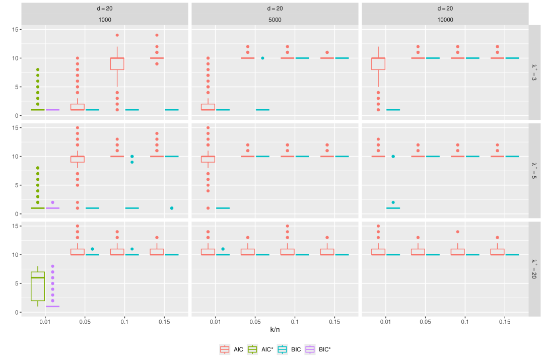
Figure 1: Simulations for the directional model with $p^{*}=10$ and dimension $d=20$: From left to the right the sample size increases from $n=1000$, $n=5000$ to $n=10000$. From top to bottom, the value of the relevant eigenvalues increases from $\lambda^{*}=3$, $\lambda^{*}=5$ to $\lambda^{*}=20$. In every subplot the ratio $k_{n}/n$ increases from left to right from $0.01$, $0.05$, $0.1$ to $0.15$. The box plots show the estimator $\widehat{p}_{n}$ for $p^{*}=10$ of the $\operatorname{AIC}$ and $\operatorname{BIC}$.

The results for $d=20$ are presented in Figure 1. The estimator $\widehat{p}_{n}$ of both information criteria gets closer to the true value $p^{*}=10$ if $k_{n}$ increases. For $n=1000$ and $k_{n}/n=0.01$, we have $k_{n}=10<d=20$ and therefore we use the $\operatorname{AIC}^{*}$ and $\operatorname{BIC}^{*}$. Both information criteria underestimate $p^{*}$, which is expected as the number of extreme observations $k_{n}$ equals $p^{*}$. In all other cases, the $\operatorname{AIC}$ and $\operatorname{BIC}$ are used. For $k_{n}/n\geq 0.05$ and $\lambda^{*}=3$, the $\operatorname{AIC}$ either estimates $p^{*}$ or shows more outliers above $p^{*}$. Overall, the $\operatorname{AIC}$ performs better, when $\lambda^{*}$ or $k_{n}$ increases. The $\operatorname{BIC}$ estimates the true value of $p^{*}$ or underestimates $p^{*}$, where the number of cases with underestimation becomes smaller when $\lambda^{*}$ or $k_{n}$ grows. This is also intuitive: for a higher value of $\lambda^{*}$ the spike is more pronounced. In comparison to the $\operatorname{AIC}$, the estimates of the $\operatorname{BIC}$ have, in general, fewer fluctuations and outliers.

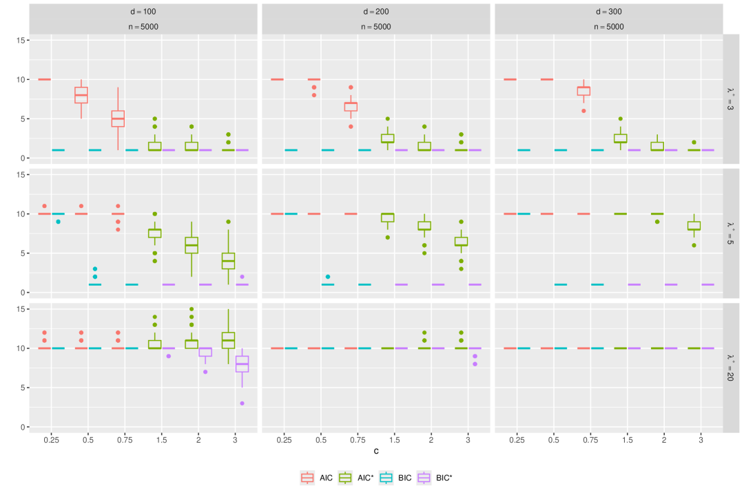
Figure 2: Simulations for directional factor data with $p^{*}=10$ and sample size $n=5000$: From left to the right the dimension increases from $d=100$, $d=200$ to $d=300$. From top to bottom, the value of the relevant eigenvalues increases from $\lambda^{*}=3$, $\lambda^{*}=5$ to $\lambda^{*}=20$. In every subplot the ratio $c=d/k_{n}$ increases from left to right from $c=0.25$, $c=0.5$, $c=0.75$, $c=1.5$, $c=2$ to $c=3$. The box plot shows the estimator $\widehat{p}_{n}$ for $p^{*}=10$ for the different information criteria.

For the high-dimensional case $d\geq 100$, Figure 2 depicts the simulation results. Note that for $\lambda^{*}=3$ the gap condition is satisfied when $c<1$, and for $\lambda^{*}=5$ and $20$ for all $c$. It should also be noted that for fixed $n$ and $d_{n}$ but increasing $c$, the number of extreme observations $k_{n}$ decreases, leading to a smaller sample size. The $\operatorname{AIC}$ and $\operatorname{AIC}^{*}$ both profit from an increase in dimension and $\lambda^{*}$. Overall, the estimates of both criteria get better for a larger dimension. In comparison to Figure 1, we see that the $\operatorname{AIC}^{*}$ has the tendency to underestimate $p^{*}$ for $\lambda^{*}\leq 5$, $c=2$ and $c=3$, which is consistent with Theorem 4.7. The estimates $\widehat{p}_{n}$ of the $\operatorname{AIC}$ and $\operatorname{AIC}^{*}$ are closer to $p^{*}$ in comparison to the $\operatorname{BIC}$ and $\operatorname{BIC}^{*}$ as soon as the gap condition is fulfilled. When the gap condition is not satisfied, the information criteria underestimate $p^{*}$, where for $c\geq 0.5$ the $\operatorname{BIC}$ and $\operatorname{BIC}^{*}$ only give usable results for $\lambda^{*}=20$. For $c>1$ the $\operatorname{BIC}^{*}$ shows underestimation in all cases.

5.2 Directional model with noise

In this example, we consider again the directional model with the same choice of distributions as in Section 5.1, but additionally, we add noise. As noise, we use the $d$-dimensional random vector

$$\boldsymbol{\varepsilon}\sim\Big{|}\mathcal{N}_{d}\Big{(}\mathbf{0}_{d},\frac{100}{d}\boldsymbol{I}_{d}\Big{)}\Big{|},$$

where the absolute value is entry-wise. Due to the scaling of the covariance matrix by $100/d$ the variance of the norm of $\boldsymbol{\varepsilon}$ converges as $d\rightarrow\infty$ to $100/\sqrt{2}$ (see Lemma D.1). Then, we construct the regularly varying random vector

$${\boldsymbol{X}}^{(n)}=\frac{\phantom{\|}{{\boldsymbol{\Gamma}}^{(n)}}^{1/2}{\boldsymbol{V}}^{(n)}\phantom{\|}}{\|{{\boldsymbol{\Gamma}}^{(n)}}^{1/2}{\boldsymbol{V}}^{(n)}\|}\cdot Z+\boldsymbol{\varepsilon}\in\mathbb{R}^{d_{n}},$$

where ${{\boldsymbol{\Gamma}}^{(n)}},{\boldsymbol{V}}^{(n)}$ and $Z$ are defined as in Section 5.1 and $\boldsymbol{\varepsilon}$ is given as above.

Figure 3: Simulations for noisy directional factor data with $p^{*}=10$ and dimension $d=20$: From left to the right the sample size increases from $n=1000$, $n=5000$ to $n=10000$. From top to bottom, the value of the relevant eigenvalues increases from $\lambda^{*}=3$, $\lambda^{*}=5$ to $\lambda^{*}=20$. In every subplot the ratio $k_{n}/n$ increases from left to right from $0.01$, $0.05$, $0.1$ to $0.15$. The box plots show the estimator $\widehat{p}_{n}$ for $p^{*}=10$ for the $\operatorname{AIC}$ and $\operatorname{BIC}$.

The results are shown for $d=20$ in Figure 3. Overall, the results are similar to Figure 1, but with more deviation from the true value $p^{*}$. In most cases (e.g. $n=5000,10000$, $k_{n}/n\geq 0.05$ and $\lambda^{*}\geq 5$), the information criteria estimated $\widehat{p}_{n}=11$ relevant eigenvalues, therefore identifying not only the 10 dominant eigenvalues but also including the noise. The noise leads to more fluctuation of the $\operatorname{AIC}$ estimates, especially to overestimation of $p^{*}$. For the $\operatorname{BIC}$ there are cases (e.g. $n=1000$, $\lambda^{*}\leq 5$ and $k_{n}/n=0.15$), where the $\operatorname{BIC}$ estimates $\widehat{p}_{n}=1$ instead $p^{*}=10$ and without noise the estimate is concentrated near $p^{*}=10$. The $\operatorname{AIC}$ does not show this behavior. The influence of the noise decreases for larger $\lambda^{*}$, resulting in a larger spike.

Figure 4: Simulations for noisy directional factor data with $p^{*}=10$ and sample size $n=5000$: From left to the right the dimension increases from $d=100$, $d=200$ to $d=300$. From top to bottom, the value of the relevant eigenvalues increases from $\lambda^{*}=3$, $\lambda^{*}=5$ to $\lambda^{*}=20$. In every subplot the ratio $c=d/k_{n}$ increases from left to right from $c=0.25$, $c=0.5$, $c=0.75$, $c=1.5$, $c=2$ to $c=3$. The box plot shows the estimator $\widehat{p}_{n}$ for $p^{*}=10$ for the different information criteria.

Figure 4 provides a visualization of the results in the high-dimensional cases $d=100$, $d=200$ and $d=300$. We see that the effect of the noise is similar to the low-dimensional case. The overall fluctuation increases compared to the simulation without noise in Figure 2. The $\operatorname{AIC}$ and $\operatorname{AIC}^{*}$ estimate the noise as an additional direction, for example, when $\lambda^{*}=20$ and $d=300$. The $\operatorname{BIC}$ and the $\operatorname{BIC}^{*}$ give as estimation $\widehat{p}_{n}=10$ in some cases (e.g. $d=100$, $\lambda^{*}=20$ and $c\geq 0.5$), therefore they are able to differentiate between the noise and the true value $p^{*}=10$.

5.3 Spiked angular Gaussian model

In this section, we consider the contaminated spiked angular Gaussian model, which can also be found in AMDS:22. For $1\leq p^{*}\leq d$ we define the regularly varying random vector

$$\boldsymbol{X}=\boldsymbol{N}Z\in\mathbb{R}^{d},$$

where $Z$ is a univariate standard Fréchet distributed random variable, $\boldsymbol{N}$ follows a $d$-dimensional centered normal distribution with covariance matrix

$$\boldsymbol{H}\coloneqq\sum_{i=1}^{p^{*}}\lambda_{i}\boldsymbol{v}_{i}\boldsymbol{v}_{i}^{\top}+\lambda\boldsymbol{I}_{d},$$

where $\boldsymbol{v}_{i},\,i=1,\ldots,{p^{*}}$ are orthogonal vectors and $\lambda_{1}\geq\lambda_{2}\geq\cdots\geq\lambda_{p^{*}}>\lambda=\cdots=\lambda>0$. Note that the distribution of $\boldsymbol{X}$ differs from the directional model in Section 5.1, since the normal distribution is not standardized when $\boldsymbol{X}$ is generated. The spectral vector arising from $\boldsymbol{X}$ concentrates on a $p$-dimensional subspace and is given by (see AMDS:22)

$$\mathbb{P}(\boldsymbol{\Theta}\in\cdot)=\frac{\mathbb{E}[\|\boldsymbol{N}\|\delta_{\boldsymbol{N}/\|\boldsymbol{N}\|}(\cdot)]}{\mathbb{E}[\|\boldsymbol{N}\|]}.$$

Figure 5: Simulations for spiked angular Gaussian data with $p^{*}=10$: From left to the right the dimension increases from $d=100$, $d=300$ to $d=900$. From top to bottom, the value of $\lambda$ increases from $\lambda=0.01$, $\lambda=0.1$ to $\lambda=1$. In every subplot the ratio $c=d/k_{n}$ increases from left to right from $c=0.25$, $c=0.5$, $c=0.75$, $c=1.5$, $c=2$ to $c=3$. The box plot is log-scaled and shows the estimator $\widehat{p}_{n}$ for the different information criteria.

For the comparison, we run simulations with sample size $n=5000$, dimension $d=100$, $d=300$ to $d=900$. The matrix $\boldsymbol{H}$ is fixed for each sample but is initially randomly generated for the simulation, where the eigenvalues $\lambda_{1}=\cdots=\lambda_{10}=20$ are equal to $20$, $p^{*}=10$ and the last eigenvalue $\lambda$ varies; we analyze the behavior of the information criteria when $\lambda$ gets closer to $0$ and thus, the spiked covariance assumption is closer to being violated. Therefore, we compare the results for $\lambda=0.01$, $\lambda=0.1,$ and $\lambda=1$. The eigenvectors $\boldsymbol{v}_{i}$ are generated with the R package pracma.

The results are illustrated in Figure 5. It is evident that, when the gap is sufficiently large, then the $\operatorname{BIC}$ and $\operatorname{BIC}^{*}$ are less affected by a small eigenvalue $\lambda$ than the $\operatorname{AIC}$ and $\operatorname{AIC}^{*}$. The smaller $\lambda$ is chosen, the larger the overestimation of the $\operatorname{AIC}$ and $\operatorname{AIC}^{*}$ is, whereby for $d=900$ and $\lambda=0.01,0.1$ the $\operatorname{AIC}^{*}$ overestimates $p^{*}$ more than $\operatorname{AIC}$. When $\lambda=1$ and $d\geq 300$ the performance of all criteria is nearly identical.

6 Application to precipitation data

In this section, the information criteria are applied to precipitation data in Germany taken from DWD. The data set consists of daily station observations of the precipitation height for Germany between January 1, 1951 and March 31, 2022 at $d=500$ stations. The stations are marked by black dots in Figure 6. The data is preprocessed to include only observations from January, February and March, and transformed to standard Fréchet margins. After data cleaning, the resultant dataset contains $n=2546$ observations, each with precipitation records from at least one station. In Figure 6 we see the stations of the empirical eigenvectors $\widehat{\boldsymbol{v}}_{i}=(v_{1}^{(i)},\ldots,v_{d}^{(i)})^{\top}$, where $v_{j}^{(i)}\geq 0.6v_{(1)}^{(i)}$, $i=1,\ldots,5$, of the 5 largest empirical eigenvalues $\widehat{\lambda}_{n,1},\ldots,\widehat{\lambda}_{n,5}$ if $k_{n}=76$; the stations of each eigenvector are colored differently.

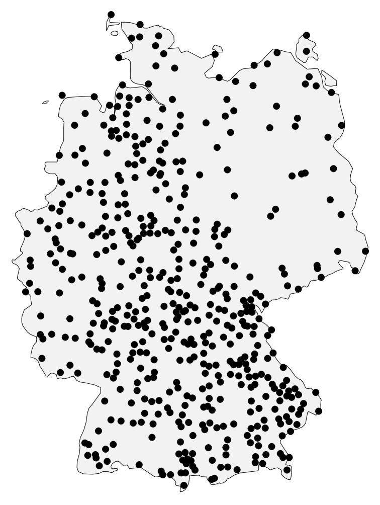
Figure 6: Left figure: Map of Germany with all stations highlighted by black dots. Right figure: Map of Germany with the most extreme stations of the empirical eigenvectors of the five largest empirical eigenvalues, colored by eigenvectors.

We consider $1\%$ to $15\%$ of the data as extreme, corresponding to $25$ to $382$ observations. In these cases $d>k_{n}$ and therefore, we assume to be in the high-dimensional setting with $c>1$ and apply $\operatorname{AIC}^{*}$ and $\operatorname{BIC}^{*}$ from Definition 4.6. The number of candidate models $q_{n}$ for the $\operatorname{AIC}^{*}$ is chosen as $d/2=250$ to account for the assumption of Theorem 4.7.

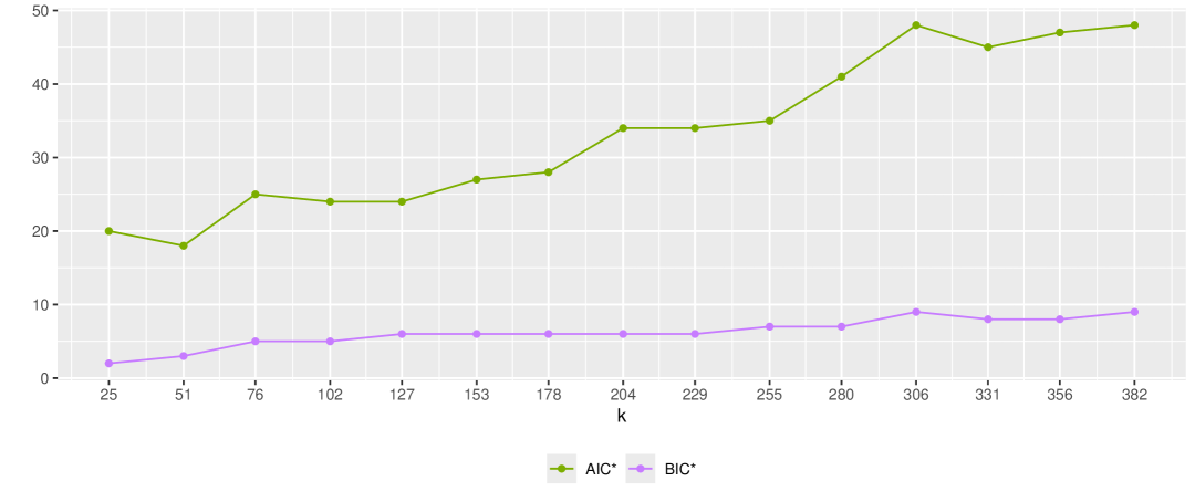
Figure 7: The estimated number $\widehat{p}_{n}$ of significant eigenvalues determined by $\operatorname{AIC}^{*}$ and $\operatorname{BIC}^{*}$ plotted against $k_{n}$.                                  

Figure 8: For $k_{n}=76$, on the left hand side the scaled ordered empirical eigenvalues $\widehat{\lambda}_{n,i}/\widehat{\lambda}_{n,1}$, $i=1,\ldots,75$ and on the right hand side the differences of the ordered empirical eigenvalues divided by the value of the largest eigenvalue $(\widehat{\lambda}_{n,i}-\widehat{\lambda}_{n,i+1})/\widehat{\lambda}_{n,1}$, $i=1,\ldots,75$ are plotted. The vertical line indicates the $\operatorname{AIC}^{*}$ estimator $\widehat{p}_{n}=25$ and the $\operatorname{BIC}^{*}$ estimator $\widehat{p}_{n}=5$.

$k_{n}$	25	51	76	102	127	153	178	204	229	255	280	306	331	356	382
$\operatorname{AIC}^{*}$	20	18	25	24	24	27	28	34	34	35	41	48	45	47	48
$\operatorname{BIC}^{*}$	2	3	5	5	6	6	6	6	6	7	7	9	8	8	9

Table 6.1: Estimated number $\widehat{p}_{n}$ of significant eigenvalues in the precipitation data for different values of $k_{n}$ and information criteria $\operatorname{AIC}^{*}$ and $\operatorname{BIC}^{*}$.

Figure 7 shows the number of estimated significant eigenvalues $\widehat{p}_{n}$ mapped against $k_{n}$. The estimates using $\operatorname{AIC}^{*}$ stabilize between $k_{n}=76$ and $k_{n}=178$, ranging from $24$ to $28$, before increasing further. In contrast, $\operatorname{BIC}^{*}$ stabilizes for $k_{n}$ between $76$ and $229$, with values of $5$ and $6$. Even for $k_{n}\geq 255$, the $\operatorname{BIC}^{*}$ remains between $7$ and $9$, whereas $\operatorname{AIC}^{*}$ continues to increase. This difference between the estimates aligns with the heavier penalty imposed by $\operatorname{BIC}^{*}$, which leads to smaller estimates compared to $\operatorname{AIC}^{*}$. These estimates reduce the dimensionality of $d=500$ by factors of $20$ and $100$, respectively. For comparison of these different estimates, the scaled empirical eigenvalues $\widehat{\lambda}_{n,i}/\widehat{\lambda}_{n,1}$, $i=1,\ldots,75$, are plotted in the left picture of Figure 8. At first view, they seem not to be constant after some point, contradicting the spiked covariance assumption. But if we investigate the scaled increments of the eigenvalues $(\widehat{\lambda}_{n,i}-\widehat{\lambda}_{n,i+1})/\widehat{\lambda}_{n,1}$, $i=1,\ldots,75$ in the right plot of Figure 8, we realize that after some point these increments are nearly constant. The information criteria seem to estimate the point where these increments are constant because in the interval $[5,24]$, which is spanned by our estimators, this happens.

7 Conclusion

The paper proposed information criteria based on the AIC and BIC for Gaussian random vectors to detect the number $p^{*}$ of significant principal components in multivariate extremes, which corresponds to the location of the spike in the eigenvalues of the covariance matrix of the angular measure. Our analysis encompassed both the classical large-sample setting and the high-dimensional setting, which has become increasingly relevant for extreme value theory in today’s applications. We established the consistency of the $\operatorname{BIC}$ in the large-sample setting and sufficient criteria for the $\operatorname{AIC}$ and the $\operatorname{BIC}$ to be consistent in the high-dimensional setting of a directional model. The results of this paper are in accordance with the results in the non-extreme world. For the proofs we derived some new results on the asymptotic properties of the empirical eigenvalues of $\boldsymbol{\Sigma}$ in both the large-dimensional case, but, in particular, in the high-dimensional case using methods from random matrix theory. The performance of the information criteria was further validated through a simulation study and a real-world example.

The case $c=0$ was not covered in that paper because the $\operatorname{AIC}$ and $\operatorname{BIC}$, as defined here, are not consistent even when a type of gap condition is satisfied. From a practical point of view, we believe that in the context of multivariate extremes, this is also not a realistic scenario because usually $k_{n}$, the number of extremes, is small, and then $d_{n}/k_{n}$ will be large.

The paper focused on eigenvalues of $\boldsymbol{\Sigma}$ that satisfy the spiked covariance structure in (1.1), where $\xi_{p^{*}}$ is a distant spiked eigenvalue in the sense that $\xi_{p^{*}}>1+\sqrt{c}$ and $c=\lim_{n\to\infty}d_{n}/k_{n}>0$. For applications, these eigenvalue assumptions are restrictive, as we see in our data example in Figure 8, where the empirical eigenvalues decrease but do not stabilize at some point. Therefore, it is worth exploring more general eigenvalue structures of the covariance matrix to estimate the number of significant components of $\boldsymbol{\Sigma}$ such as, e.g., $\xi_{p^{*}}>1+\sqrt{c}$ and $\xi_{p^{*}+1}<1+\sqrt{c}$ where all eigenvalues $\xi_{j}$ for $j=p^{*}+1,\ldots,d_{n}$ are in a neighborhood of $1$ or $0$.

Additionally, as a starting point of this line of research on PCA for high-dimensional extremes, the consistency results of the information criteria were based on the assumption that the underlying model is a directional model, similar to multivariate statistics, where the first results were derived for Gaussian models with a special covariance structure. Of course, it would also be interesting to explore generalizations or alternatives to the directional model.

Finally, we would like to point out that changing $k_{n}$ changes not only the $\operatorname{AIC}$ and $\operatorname{BIC}$ estimators $\widehat{p}_{n}$, but also the empirical eigenvalues and hence, the scree plot as in Figure 8. Therefore, the optimal choice of $k_{n}$ is nontrivial in this context, and some further research, as discussed in [butsch2024fasen] and [meyer_muscle23] for the choice of $k_{n}$ is needed.

Appendix A Proofs of Section 2

Proof of Theorem 2.3.

1. We use Theorem A.46 in Bai:Silverstein:2010, which states that for Hermitian matrices ${\boldsymbol{A}},\boldsymbol{B}\in\mathbb{R}^{d\times d}$ with eigenvalues $\lambda_{i}({\boldsymbol{A}})$ and $\lambda_{i}(\boldsymbol{B})$, $i=1,\ldots,d$, the inequality

   $$\max_{i=1,\ldots,d}|\lambda_{i}({\boldsymbol{A}})-\lambda_{i}(\boldsymbol{B})|\leq\|{\boldsymbol{A}}-\boldsymbol{B}\|$$ (A.1)

   holds. A conclusion from Proposition 2.1 is that $\sqrt{k_{n}}(\widehat{\boldsymbol{\Sigma}}_{n}-\boldsymbol{\Sigma})=O_{\mathbb{P}}(1)$ and therefore A.1 yields

   $$(\widehat{\lambda}_{n,1},\ldots,\widehat{\lambda}_{n,d-1})=(\lambda_{1},\ldots,\lambda_{d-1})+O_{\mathbb{P}}(1/\sqrt{k_{n}}).$$

2. The result corresponds to Dauxois:Pousse:Romain:1982, which is based on a similar convergence as Proposition 2.1.

∎

Proof of Lemma 2.5.

Note that

$${\boldsymbol{\Sigma}}^{(n)}=\operatorname{Cov}({\boldsymbol{\Theta}}^{(n)})={{{\boldsymbol{\Gamma}}^{(n)}}}^{1/2}\operatorname{Cov}\left(\frac{{\boldsymbol{V}}^{(n)}}{\|{{{\boldsymbol{\Gamma}}^{(n)}}}^{1/2}{\boldsymbol{V}}^{(n)}\|}\right){{{\boldsymbol{\Gamma}}^{(n)}}}^{1/2}.$$

Utilizing the spectral decomposition ${{\boldsymbol{\Gamma}}^{(n)}}={\boldsymbol{W}}^{(n)}{\boldsymbol{D}^{(n)}}{{\boldsymbol{W}}^{(n)}}^{\top},$ where ${\boldsymbol{W}}^{(n)}=({\boldsymbol{W}}^{(n)}_{1},\ldots,$ ${\boldsymbol{W}}^{(n)}_{d_{n}})$ is a $d_{n}\times d_{n}$-dimensional orthogonal matrix and

$${\boldsymbol{D}^{(n)}}\coloneqq\operatorname{diag}(\overline{\boldsymbol{D}}_{n},\boldsymbol{I}_{d_{n}-p^{*}}):=\operatorname{diag}(\xi_{n,1},\ldots,\xi_{n,p^{*}},1,\ldots,1)\in\mathbb{R}^{d_{n}\times d_{n}}$$

is a diagonal matrix consisting of the eigenvalues of ${{\boldsymbol{\Gamma}}^{(n)}}$, we receive with $\|{\boldsymbol{W}}^{(n)}\boldsymbol{x}\|=\|\boldsymbol{x}\|$ for $\boldsymbol{x}\in\mathbb{R}^{d_{n}}$ that

$${\boldsymbol{\Sigma}}^{(n)}=\operatorname{Cov}\left(\frac{{{{\boldsymbol{\Gamma}}^{(n)}}}^{1/2}{\boldsymbol{V}}^{(n)}}{\|{{{\boldsymbol{\Gamma}}^{(n)}}}^{1/2}{\boldsymbol{V}}^{(n)}\|}\right) ={\boldsymbol{W}}^{(n)}\operatorname{Cov}\left(\frac{{{\boldsymbol{D}^{(n)}}}^{1/2}{\boldsymbol{V}}^{(n)}}{\|{{\boldsymbol{D}^{(n)}}}^{1/2}{\boldsymbol{V}}^{(n)}\|}\right){{\boldsymbol{W}}^{(n)}}^{\top}.$$

Hence, the matrices

$$\operatorname{Cov}\left(\frac{{{{\boldsymbol{\Gamma}}^{(n)}}}^{1/2}{\boldsymbol{V}}^{(n)}}{\|{{{\boldsymbol{\Gamma}}^{(n)}}}^{1/2}{\boldsymbol{V}}^{(n)}\|}\right)\quad\text{ and }\quad\operatorname{Cov}\left(\frac{{{\boldsymbol{D}^{(n)}}}^{1/2}{\boldsymbol{V}}^{(n)}}{\|{{\boldsymbol{D}^{(n)}}}^{1/2}{\boldsymbol{V}}^{(n)}\|}\right)$$

are similar and share the same eigenvalues (matrix_analysis). Therefore, we assume in the following w.l.o.g. that ${{\boldsymbol{\Gamma}}^{(n)}}={\boldsymbol{D}^{(n)}}$ and hence,

$${\boldsymbol{\Sigma}}^{(n)}=\operatorname{Cov}\left(\frac{{{\boldsymbol{D}^{(n)}}}^{1/2}{\boldsymbol{V}}^{(n)}}{\|{{\boldsymbol{D}^{(n)}}}^{1/2}{\boldsymbol{V}}^{(n)}\|}\right)$$

is a diagonal matrix. Indeed, since ${\boldsymbol{D}^{(n)}}$ is a diagonal matrix and $V_{1},\ldots,V_{d_{n}}$ are symmetric and i.i.d., the components of ${{\boldsymbol{D}^{(n)}}}^{1/2}{\boldsymbol{V}}^{(n)}/\|{{\boldsymbol{D}^{(n)}}}^{1/2}{\boldsymbol{V}}^{(n)}\|$ are uncorrelated. Further, the eigenvalues of ${\boldsymbol{\Sigma}}^{(n)}$ are the diagonal entries

$$\operatorname{diag}({\boldsymbol{\Sigma}}^{(n)})_{i}=\mathbb{E}\left[\frac{\xi_{n,i}V_{i}^{2}}{\|{{{\boldsymbol{\Gamma}}^{(n)}}}^{1/2}{\boldsymbol{V}}^{(n)}\|^{2}}\right]=\mathbb{E}\left[\frac{\xi_{n,i}V_{i}^{2}}{\sum_{j=1}^{p^{*}}\xi_{n,j}V_{j}^{2}+\sum_{j=p^{*}+1}^{d_{n}}V_{j}^{2}}\right],\quad i=1,\ldots,p^{*}$$

and

$$\operatorname{diag}({\boldsymbol{\Sigma}}^{(n)})_{i}=\operatorname{diag}({\boldsymbol{\Sigma}}^{(n)})_{d_{n}}=\mathbb{E}\left[\frac{V_{d_{n}}^{2}}{\sum_{j=1}^{p^{*}}\xi_{n,j}V_{j}^{2}+\sum_{j=p^{*}+1}^{d_{n}}V_{j}^{2}}\right],\quad i=p^{*}+1,\ldots,d_{n},$$

which has multiplicity $(d_{n}-p^{*})$. For $1\leq i\leq p^{*}$ and $l>p^{*}$, the function

$$\frac{\xi V_{i}^{2}-V_{l}^{2}}{\xi V_{i}^{2}+\sum_{\begin{subarray}{c}j=1\\ j\neq i\end{subarray}}^{p^{*}}\xi_{n,j}V_{j}^{2}+\sum_{j=p^{*}+1}^{d_{n}}V_{j}^{2}}$$

is strictly increasing function in $\xi$ since the derivative in $\xi$ is strictly positive. A conclusion is then for $1\leq i\leq p^{*}$ with $\xi_{n,i}>1$ and $l>p^{*}$ that

$$\operatorname{diag}({\boldsymbol{\Sigma}}^{(n)})_{i}-\operatorname{diag}({\boldsymbol{\Sigma}}^{(n)})_{l} =\mathbb{E}\left[\frac{\xi_{n,i}V_{i}^{2}-V_{l}^{2}}{\sum_{j=1}^{p^{*}}\xi_{n,p^{*}}V_{j}^{2}+\sum_{j=p^{*}+1}^{d_{n}}V_{j}^{2}}\right]$$

$$>\mathbb{E}\left[\frac{V_{i}^{2}-V_{l}^{2}}{\sum_{\begin{subarray}{c}j=1\\ j\neq i\end{subarray}}^{p^{*}}\xi_{n,p^{*}}V_{j}^{2}+V_{i}^{2}+\sum_{j=p^{*}+1}^{d_{n}}V_{j}^{2}}\right]=0.$$

Therefore, we receive that the first $p^{*}$ diagonal entries of ${\boldsymbol{\Sigma}}^{(n)}$ correspond to the $p^{*}$ largest eigenvalues of ${\boldsymbol{\Sigma}}^{(n)}$ namely $\operatorname{diag}({\boldsymbol{\Sigma}}^{(n)})_{1}$, …, $\operatorname{diag}({\boldsymbol{\Sigma}}^{(n)})_{p^{*}}$ and the remaining $(d_{n}-p^{*})$ eigenvalues are strictly smaller and identical to $\operatorname{diag}({\boldsymbol{\Sigma}}^{(n)})_{d_{n}}$. ∎

A.1 Proof of Theorem 2.7

For the proof of Theorem 2.7 we combine ideas for the spiked covariance model from johnstone:2018 and for compositional data from jiang:2023. First, we derive an alternative representation for ${\widehat{\boldsymbol{\Sigma}}}{}^{(n)}$ in 2.4. As a consequence of the independence between the radial components $Z_{1},\ldots,Z_{n}$ and the directional components ${\boldsymbol{X}}^{(n)}_{1}/\|{\boldsymbol{X}}^{(n)}_{1}\|,\ldots,{\boldsymbol{X}}^{(n)}_{k_{n}}/\|{\boldsymbol{X}}^{(n)}_{k_{n}}\|$ we obtain

$$\widehat{\boldsymbol{\Theta}}{}^{(n)} =\sum_{j=1}^{n}\frac{{{\boldsymbol{\Gamma}}^{(n)}}^{1/2}{\boldsymbol{V}}^{(n)}_{j}}{\|{{\boldsymbol{\Gamma}}^{(n)}}^{1/2}{\boldsymbol{V}}^{(n)}_{j}\|}\mathbbm{1}\{Z_{j}>Z_{(k_{n}+1,n)}\}\overset{\mathcal{D}}{=}\sum_{j=1}^{k_{n}}\frac{{\boldsymbol{X}}^{(n)}_{j}}{\|{\boldsymbol{X}}^{(n)}_{j}\|},$$

and similarly

$$\widehat{\boldsymbol{\Sigma}}{}^{(n)\prime}\coloneqq{} \frac{1}{k_{n}}\sum_{j=1}^{k_{n}}\left(\frac{{\boldsymbol{X}}^{(n)}_{j}}{\|{\boldsymbol{X}}^{(n)}_{j}\|}-\frac{1}{k_{n}}\sum_{i=1}^{k_{n}}\frac{{\boldsymbol{X}}^{(n)}_{i}}{\|{\boldsymbol{X}}^{(n)}_{i}\|}\right)\left(\frac{{\boldsymbol{X}}^{(n)}_{j}}{\|{\boldsymbol{X}}^{(n)}_{j}\|}-\frac{1}{k_{n}}\sum_{i=1}^{k_{n}}\frac{{\boldsymbol{X}}^{(n)}_{i}}{\|{\boldsymbol{X}}^{(n)}_{i}\|}\right)^{\top}\overset{\mathcal{D}}{=}{}{\widehat{\boldsymbol{\Sigma}}}{}^{(n)}.$$ (A.2)

The eigenvalues of $\widehat{\boldsymbol{\Sigma}}{}^{(n)\prime}$ are denoted by $\widehat{\lambda}_{n,1}^{\prime},\ldots,\widehat{\lambda}_{n,d_{n}}^{\prime}$ and due to A.2 we receive that

$$(\widehat{\lambda}_{n,1}^{\prime},\ldots,\widehat{\lambda}_{n,d_{n}}^{\prime})\overset{\mathcal{D}}{=}(\widehat{\lambda}_{n,1},\ldots,\widehat{\lambda}_{n,d_{n}}).$$ (A.3)

Thus, to prove Theorem 2.7 it suffices to derive the asymptotic behavior of $(\widehat{\lambda}_{n,1}^{\prime},\ldots,\widehat{\lambda}_{n,d_{n}}^{\prime})$, which relies on the spectral analysis of the empirical covariance matrix of ${{\boldsymbol{\Gamma}}^{(n)}}^{1/2}{\boldsymbol{V}}^{(n)}$. Therefore, assume that ${\boldsymbol{V}}^{(n)}_{1},\ldots,{\boldsymbol{V}}^{(n)}_{k_{n}}$ is an i.i.d. sequence with distribution ${\boldsymbol{V}}^{(n)}$, i.e. ${\boldsymbol{V}}^{(n)}_{i}\in\mathbb{R}^{d_{n}}$ has i.i.d. entries with mean $0$ and variance $1$. Then we define the sequence of matrices

$$\boldsymbol{\Upsilon}^{(n)}\coloneqq\frac{1}{k_{n}}\sum_{i=1}^{k_{n}} \bigg{(}{{\boldsymbol{\Gamma}}^{(n)}}^{1/2}{\boldsymbol{V}}^{(n)}_{i}-\frac{1}{k_{n}}\sum_{j=1}^{k_{n}}{{\boldsymbol{\Gamma}}^{(n)}}^{1/2}{\boldsymbol{V}}^{(n)}_{j}\bigg{)}$$

$$\quad\cdot\bigg{(}{{\boldsymbol{\Gamma}}^{(n)}}^{1/2}{\boldsymbol{V}}^{(n)}_{i}-\frac{1}{k_{n}}\sum_{j=1}^{k_{n}}{{\boldsymbol{\Gamma}}^{(n)}}^{1/2}{\boldsymbol{V}}^{(n)}_{j}\bigg{)}^{\top},\quad n\in\mathbb{N},$$ (A.4)

whose eigenvalues are denoted by $\widehat{\xi}_{n,1}>\cdots>\widehat{\xi}_{n,d_{n}}>0$. The aim now is to write $\widehat{\boldsymbol{\Sigma}}{}^{(n)\prime}$ and $\boldsymbol{\Upsilon}^{(n)}$ as matrix products. Therefore, define

$${\mathcal{V}}^{(n)}\coloneqq({\boldsymbol{V}}^{(n)}_{1},\ldots,{\boldsymbol{V}}^{(n)}_{k_{n}})\in\mathbb{R}^{d_{n}\times k_{n}}$$

and

$${\boldsymbol{T}}^{(n)}\coloneqq\operatorname{diag}(\|{{\boldsymbol{\Gamma}}^{(n)}}^{1/2}{\boldsymbol{V}}^{(n)}_{1}\|^{-1},\ldots,\|{{\boldsymbol{\Gamma}}^{(n)}}^{1/2}{\boldsymbol{V}}^{(n)}_{k_{n}}\|^{-1})\in\mathbb{R}^{k_{n}\times k_{n}},$$

which allows us to write

$$\biggl{(}\frac{{\boldsymbol{X}}^{(n)}_{1}}{\|{\boldsymbol{X}}^{(n)}_{1}\|},\ldots,\frac{{\boldsymbol{X}}^{(n)}_{k_{n}}}{\|{\boldsymbol{X}}^{(n)}_{k_{n}}\|}\biggr{)}^{\top} ={{\boldsymbol{\Gamma}}^{(n)}}^{1/2}{\mathcal{V}}^{(n)}{\boldsymbol{T}}^{(n)}.$$

Finally, with the projection matrix ${{\boldsymbol{P}}^{(n)}}\coloneqq(\boldsymbol{I}_{k_{n}}-\mathbf{1}_{k_{n}}\mathbf{1}_{k_{n}}^{\top}/{k_{n}})$, the matrices $\widehat{\boldsymbol{\Sigma}}{}^{(n)\prime}$ and $\boldsymbol{\Upsilon}^{(n)}$, as defined in A.4 and A.2, can be written as

$$\widehat{\boldsymbol{\Sigma}}{}^{(n)\prime} =\frac{1}{k_{n}}({{\boldsymbol{\Gamma}}^{(n)}}^{1/2}{\mathcal{V}}^{(n)}{\boldsymbol{T}}^{(n)}{{\boldsymbol{P}}^{(n)}})({{\boldsymbol{\Gamma}}^{(n)}}^{1/2}{\mathcal{V}}^{(n)}{\boldsymbol{T}}^{(n)}{{\boldsymbol{P}}^{(n)}})^{\top},$$ (A.5)

$$\boldsymbol{\Upsilon}^{(n)} =\frac{1}{k_{n}}({{\boldsymbol{\Gamma}}^{(n)}}^{1/2}{\mathcal{V}}^{(n)}{{\boldsymbol{P}}^{(n)}})({{\boldsymbol{\Gamma}}^{(n)}}^{1/2}{\mathcal{V}}^{(n)}{{\boldsymbol{P}}^{(n)}})^{\top}.$$

In the following theorem the connection between the eigenvalues $\widehat{\xi}_{n,i}$ and $d_{n}\widehat{\lambda}^{\prime}_{n,i}$ is derived.

Theorem A.1.

Let Model B be given. Suppose that $\boldsymbol{\Gamma}_{n}\rightarrow\boldsymbol{\Gamma}$ and $(\xi_{n,1},\ldots,\xi_{n,p^{*}})\rightarrow(\xi_{1},\ldots,\xi_{p^{*}})$ as $n\to\infty$. If $\widehat{\xi}_{n,1},\ldots,\widehat{\xi}_{n,d_{n}}$ denote the eigenvalues of $\boldsymbol{\Upsilon}^{(n)}$ in A.4 and $\widehat{\lambda}^{\prime}_{n,1},\ldots,\widehat{\lambda}^{\prime}_{n,d_{n}}$ denote the eigenvalues of $\widehat{\boldsymbol{\Sigma}}{}^{(n)\prime}$ in A.2, then as $n\to\infty$,

$$\max_{1\leq i\leq d_{n}}\big{|}\widehat{\xi}_{n,i}-d_{n}\widehat{\lambda}^{\prime}_{n,i}\big{|}\overset{\mathbb{P}}{\longrightarrow}0.$$

Proof of Theorem A.1.

Due to Theorem A.46 in Bai:Silverstein:2010 and the sub-multiplicativity of the spectral norm we receive that

$$\max_{1\leq i\leq d_{n}}\left|\sqrt{\widehat{\xi}_{n,i}}-\sqrt{d_{n}\widehat{\lambda}^{\prime}_{n,i}}\right| \leq\left\|\frac{\sqrt{d_{n}}{{\boldsymbol{\Gamma}}^{(n)}}^{1/2}{\mathcal{V}}^{(n)}{\boldsymbol{T}}^{(n)}{{\boldsymbol{P}}^{(n)}}}{\sqrt{k_{n}}}-\frac{{{\boldsymbol{\Gamma}}^{(n)}}^{1/2}{\mathcal{V}}^{(n)}{{\boldsymbol{P}}^{(n)}}}{\sqrt{k_{n}}}\right\|$$

$$\leq\left\|{{\boldsymbol{P}}^{(n)}}\right\|\cdot\left\|\sqrt{d_{n}}{\boldsymbol{T}}^{(n)}-\boldsymbol{I}_{k_{n}}\right\|\cdot\left\|\frac{{{\boldsymbol{\Gamma}}^{(n)}}^{1/2}{\mathcal{V}}^{(n)}}{\sqrt{k_{n}}}\right\|$$

$$=\left\|\sqrt{d_{n}}{\boldsymbol{T}}^{(n)}-\boldsymbol{I}_{k_{n}}\right\|\cdot\left\|\frac{{{\boldsymbol{\Gamma}}^{(n)}}^{1/2}{\mathcal{V}}^{(n)}}{\sqrt{k_{n}}}\right\|=:J_{n}\cdot H_{n},$$ (A.6)

where we used that the spectral norm of ${{\boldsymbol{P}}^{(n)}}$ is bounded by $1$, because the only eigenvalues of ${{\boldsymbol{P}}^{(n)}}$ are $1$ and $0$ as ${{\boldsymbol{P}}^{(n)}}$ is a projection matrix.

Step 1. First, we show that $J_{n}$ in (A.6) converges to $0$ in probability. Therefore, we use the partitioning of the random vector ${{\boldsymbol{\Gamma}}^{(n)}}^{1/2}{\boldsymbol{V}}^{(n)}_{j}$ into the first $p^{*}$ dependent entries and the remaining $d_{n}-p^{*}$ independent entries

$${{\boldsymbol{\Gamma}}^{(n)}}^{1/2}{\boldsymbol{V}}^{(n)}_{j}=\begin{pmatrix}\boldsymbol{\Gamma}_{n}^{1/2}{\boldsymbol{V}}^{(n)}_{j,\{1,\ldots,p^{*}\}}\\ {\boldsymbol{V}}^{(n)}_{j,\{p^{*}+1,\ldots,d_{n}\}}\end{pmatrix}\eqqcolon\begin{pmatrix}(U^{(n)}_{j,1},\ldots,U^{(n)}_{j,p^{*}})^{\top}\\ (V_{j,(p^{*}+1)},\ldots,V_{j,d_{n}})^{\top}\end{pmatrix}.$$

The eigenvalues of $(\sqrt{d_{n}}{\boldsymbol{T}}^{(n)}-\boldsymbol{I}_{k_{n}})$ correspond to the the diagonal entries. Since we apply the spectral norm, we receive that

$$J_{n}^{1/2}=\left\|\sqrt{d_{n}}{\boldsymbol{T}}^{(n)}-\boldsymbol{I}_{k_{n}}\right\|^{1/2}=\max_{1\leq i\leq k_{n}}\left|\frac{\sqrt{d_{n}}}{\big{(}\sum_{l=1}^{p^{*}}{U^{(n)}_{i,l}}^{2}+\sum_{l={p^{*}}+1}^{d_{n}}{V_{i,l}}^{2}\big{)}^{1/2}}-1\right|.$$

On the one hand, by $\mathbb{E}[{V_{i,j}}^{2}]=1,d_{n}/k_{n}\rightarrow c>0$ and Bai:Yin:1993 we obtain that as $n\to\infty$

$$\max_{1\leq i\leq k_{n}}\left|\frac{\sum_{l={p^{*}}+1}^{d_{n}}{V_{i,l}}^{2}}{d_{n}}-1\right|\overset{\mathbb{P}\text{-a.s.}}{\longrightarrow}0.$$

On the other hand, for $1\leq i\leq k_{n}$,

$$\sum_{l=1}^{p^{*}}{U^{(n)}_{i,l}}^{2}=\|\boldsymbol{\Gamma}_{n}^{1/2}{\boldsymbol{V}}^{(n)}_{i,\{1,\ldots,p^{*}\}}\|^{2}\leq\|\boldsymbol{\Gamma}_{n}^{1/2}\|^{2}\|{\boldsymbol{V}}^{(n)}_{i,\{1,\ldots,p^{*}\}}\|^{2}={\xi_{n,1}}{\sum_{l=1}^{p^{*}}{V_{i,l}}^{2}}.$$

Since the second moment of $V_{1}^{2}$ exists, we can conclude from Markov inequality for $\varepsilon>0$

$$\mathbb{P}\left(\frac{\xi_{n,1}}{d_{n}}\max_{1\leq i\leq k_{n}}\left|\sum_{l=1}^{p^{*}}{V_{i,l}}^{2}\right|>\varepsilon\right) \leq\sum_{i=1}^{k_{n}}\mathbb{P}\left(\left|\sum_{l=1}^{p^{*}}{V_{i,l}}^{2}\right|>\frac{d_{n}}{\xi_{n,1}}\varepsilon\right)$$

$$=k_{n}\mathbb{P}\left(\left|\sum_{l=1}^{p^{*}}{V_{1,l}}^{2}\right|>\frac{d_{n}}{\xi_{n,1}}\varepsilon\right)$$

$$\leq k_{n}\frac{\xi_{n,1}^{2}}{d_{n}^{2}\varepsilon^{2}}\mathbb{E}\left|\sum_{l=1}^{p^{*}}{V_{1,l}}^{2}\right|^{2},$$ (A.7)

where the right-hand side converges to $0$ as $n\to\infty$, since $k_{n}/d_{n}\to c^{-1}$ and $\xi_{n,1}^{2}/d_{n}\to 0$ as $n\to\infty$. Therefore, we get

$$\max_{1\leq i\leq k_{n}}\left|\frac{\sum_{l=1}^{p^{*}}{U^{(n)}_{i,l}}^{2}}{d_{n}}\right| \leq\frac{\xi_{n,1}}{d_{n}}\max_{1\leq i\leq k_{n}}\left|\sum_{l=1}^{p^{*}}{V_{i,l}}^{2}\right|\overset{\mathbb{P}}{\longrightarrow}0.$$

To summarize,

$$\max_{1\leq i\leq k_{n}} \left|\left(\frac{\sum_{l=1}^{p^{*}}{U^{(n)}_{i,l}}^{2}+\sum_{l={p^{*}}+1}^{d_{n}}{V_{i,l}}^{2}}{d_{n}}\right)-1\right|$$

$$\leq\max_{1\leq i\leq k_{n}}\left|\left(\frac{\sum_{l=1}^{p^{*}}{U^{(n)}_{i,l}}^{2}}{d_{n}}\right)\right|+\max_{1\leq i\leq k_{n}}\left|\left(\frac{\sum_{l={p^{*}}+1}^{d_{n}}{V_{i,l}}^{2}}{d_{n}}\right)-1\right|\overset{\mathbb{P}}{\longrightarrow}0.$$

Finally, by the mean value theorem the inequality

$$\left|1-1/\sqrt{x}\right|\leq 2\left|x-1\right|\quad\text{ for }x>\frac{1}{2}$$

holds and hence, as $n\to\infty$,

$$J_{n}^{1/2}=\max_{1\leq i\leq k_{n}}\left|1-\left(\frac{1}{d_{n}}\sum_{l=1}^{p^{*}}{U^{(n)}_{i,l}}^{2}+\frac{1}{d_{n}}\sum_{l={p^{*}}+1}^{d_{n}}{V_{i,l}}^{2}\right)^{-1/2}\right|\overset{\mathbb{P}}{\longrightarrow}0.$$ (A.8)

Step 2. Next, we show that $H_{n}$ in (A.6) is $\mathbb{P}$-a.s. bounded. By yin:bai:krishnaiah:1988 (cf. Bai:Silverstein:2010)

$$H_{n}=\left\|\frac{{{\boldsymbol{\Gamma}}^{(n)}}^{1/2}{\mathcal{V}}^{(n)}}{\sqrt{k_{n}}}\right\|\leq\left\|{{\boldsymbol{\Gamma}}^{(n)}}^{1/2}\right\|\cdot\left\|\frac{{\mathcal{V}}^{(n)}}{\sqrt{k_{n}}}\right\|^{2}=\xi_{n,1}\frac{\lambda_{\text{max}}({{\mathcal{V}}^{(n)}}^{\top}{\mathcal{V}}^{(n)})}{k_{n}}\overset{\mathbb{P}\text{-a.s.}}{\longrightarrow}\xi_{1}$$

as $n\to\infty$, where $\lambda_{\text{max}}(\cdot)$ denotes the largest eigenvalue of a matrix.

Finally, a combination of (A.6), Step 1 and Step 2 result in the statement. ∎

Remark A.2.

For the convergence of the right-hand side of A.7 and hence, (A.8) to zero, it is not necessary that $\xi_{n,1}$ is bounded; it is sufficient that $\xi_{n,1}=o(\sqrt{d_{n}})$ as $n\to\infty$. But if all moments of $V_{1}$ exist, it is even sufficient to assume that $\xi_{n,1}=o(d_{n}^{\beta})$ as $n\to\infty$ for some $\beta<1$. Indeed, we get analog to A.7 for $\varepsilon>0$ that

$$\mathbb{P}\left(\frac{\xi_{n,1}}{d_{n}}\max_{1\leq i\leq k_{n}}\left|\sum_{l=1}^{p^{*}}{V_{i,l}}^{2}\right|>\varepsilon\right) \leq k_{n}\frac{\xi_{n,1}^{1/(1-\beta)}}{d_{n}^{1/(1-\beta)}}\varepsilon^{1/(1-\beta)}\mathbb{E}\left[\left|\sum_{l=1}^{p^{*}}{V_{1,l}}^{2}\right|^{1/(1-\beta)}\right]\to 0$$

as $n\to\infty$, since $k_{n}/d_{n}\to c$ and $\xi_{n,1}^{(1-\beta)^{-1}}/d_{n}^{(1-\beta)^{-1}-1}=(\xi_{n,1}/d_{n}^{\beta})^{1/(1-\beta)}=o(1)$ as $n\to\infty$.

Next, we repeat results on the asymptotic distribution of the eigenvalues of $\boldsymbol{\Upsilon}^{(n)}$ which is mainly based on Bai:Yao:2012 and Bai:Choi:Fujikoshi:2018.

Lemma A.3.

Let Model B be given. Suppose that $\boldsymbol{\Gamma}_{n}\rightarrow\boldsymbol{\Gamma}$ and $(\xi_{n,1},\ldots,\xi_{n,p^{*}})\rightarrow(\xi_{1},\ldots,\xi_{p^{*}})$ as $n\to\infty$ with $\xi_{p^{*}}>1+\sqrt{c}$. Then the following statements hold.

1. If $1\leq i\leq p^{*}$ (i.e. $\xi_{i}>1+\sqrt{c}$), then $\widehat{\xi}_{n,i}\overset{\mathbb{P}\text{-a.s.}}{\longrightarrow}\varphi_{c}(\xi_{i})$ as $n\to\infty$.

2. Define $l^{*}:=0$ if $c\leq 1$ and $l^{*}:=1-c^{-1}$ if $c>1$. Then

   $$\lim_{n\to\infty}\sup_{\alpha\in(l^{*},1)}\left|F^{\boldsymbol{\Upsilon}^{(n)}\,\leftarrow}(\alpha)-F_{c}^{\leftarrow}(\alpha)\right|=0\quad\mathbb{P}\text{-a.s.},$$

   where $F^{\boldsymbol{\Upsilon}^{(n)}\,\leftarrow}$ is the generalized inverse of the empirical spectral distribution function of $\boldsymbol{\Upsilon}^{(n)}$ and $F_{c}(x)$ is defined as in Theorem 2.7.

3. If $i_{n}(\alpha)>p^{*}$ (i.e. $\xi_{i_{n}(\alpha)}=1$) and $i_{n}(\alpha)/d_{n}\rightarrow\alpha\in(0,1)$ as $n\to\infty$, then

   $$\sup_{\alpha\in(0,1)}\left|\widehat{\xi}_{n,i_{n}(\alpha)}-F^{\leftarrow}_{c}(1-\alpha)\right| \overset{\mathbb{P}\text{-a.s.}}{\longrightarrow}0,\quad\text{ as }n\to\infty.$$

   In particular, if $(q_{n})_{n\in\mathbb{N}}$ is a sequence in $\mathbb{N}$ with $q_{n}=o(d_{n})$ as $n\to\infty$ and $q_{n}>p^{*}$, then $\widehat{\xi}_{n,q_{n}}\overset{\mathbb{P}\text{-a.s.}}{\longrightarrow}(1+\sqrt{c})^{2}$.

4. Suppose $0<c\leq 1$ and $(q_{n})_{n\in\mathbb{N}}$ is a sequence in $\mathbb{N}$ with $q_{n}=o(d_{n})$ as $n\to\infty$. Then as $n\to\infty$,

   $$\frac{1}{d_{n}-q_{n}}\sum_{i=q_{n}+1}^{d_{n}}\widehat{\xi}_{n,i}\overset{\mathbb{P}\text{-a.s.}}{\longrightarrow}1$$

   and for $q_{n}>p^{*}$ we receive that $\widehat{\xi}_{n,q_{n}}\overset{\mathbb{P}\text{-a.s.}}{\longrightarrow}(1+\sqrt{c})^{2}$.

5. Suppose $c>1$ and $(q_{n})_{n\in\mathbb{N}}$ is a sequence in $\mathbb{N}$ with $q_{n}=o(d_{n})$ as $n\to\infty$. Then as $n\to\infty$,

   $$\frac{1}{k_{n}-q_{n}}\sum_{i=q_{n}+1}^{k_{n}}\widehat{\xi}_{n,i}\overset{\mathbb{P}\text{-a.s.}}{\longrightarrow}c$$

   and for $q_{n}>p^{*}$ we receive that $\widehat{\xi}_{n,q_{n}}\overset{\mathbb{P}\text{-a.s.}}{\longrightarrow}(1+\sqrt{c})^{2}$.

Proof.

1. When the eigenvalues $(\xi_{n,1},\ldots,\xi_{n,p^{*}})=(\xi_{1},\ldots,\xi_{p^{*}})$ do not depend on $n$, (a) goes back to Bai:Yao:2012 (cf. Bai:Choi:Fujikoshi:2018). In the case $\boldsymbol{\Gamma}_{n}\rightarrow\boldsymbol{\Gamma}$ and $(\xi_{n,1},\ldots,\xi_{n,p^{*}})\rightarrow(\xi_{1},\ldots,\xi_{p^{*}})$ as $n\to\infty$ the assertion also holds because by Bai:Silverstein:2010 it can be shown with the same arguments as before that

   $$\max_{1\leq i\leq p^{*}} \left|\sqrt{\widehat{\xi}_{n,i}(\boldsymbol{\Gamma}_{n})}-\sqrt{\widehat{\xi}_{n,i}(\boldsymbol{\Gamma})}\right|\leq\|\boldsymbol{\Gamma}_{n}-\boldsymbol{\Gamma}\|\left\|\frac{{\mathcal{V}}^{(n)}}{\sqrt{k_{n}}}\right\|\|{{\boldsymbol{P}}^{(n)}}\|\overset{\mathbb{P}\text{-a.s.}}{\longrightarrow}0,$$

   where $\widehat{\xi}_{n,i}(\boldsymbol{\Gamma}_{n})$ and $\widehat{\xi}_{n,i}(\boldsymbol{\Gamma})$ is the empirical eigenvalue when $\boldsymbol{\Gamma}_{n}$ and $\boldsymbol{\Gamma}$, respectively is used.

2. The second part is similar to Bai:Yao:2012 however, the wording is not clear and therefore we prefer to include the proper statement and proof here. Note, if $d_{n}/k_{n}\rightarrow c>0$ as $n\to\infty$, then for almost all $\omega\in\Omega$, $F^{\boldsymbol{\Upsilon}^{(n)}}(\omega)$ converges in distribution to $F_{c}$ (cf. Bai:Choi:Fujikoshi:2018, silverstein:1995). This means that there exists a set $\Omega_{0}\in\mathcal{F}$ with $\mathbb{P}(\Omega_{0})=1$ and for any $\omega\in\Omega_{0}$ and any continuity point $x\in\mathbb{R}$ of $F_{c}$,

   $$\lim_{n\to\infty}F^{\boldsymbol{\Upsilon}^{(n)}}(x,\omega)=F_{c}(x).$$

   Since the distribution function $F_{c}$ is continuous on the interval $I:=((1-\sqrt{c})^{2},(1+\sqrt{c})^{2})$, a conclusion of Polya’s Theorem is the uniform convergence

   $$\lim_{n\to\infty}\sup_{x\in I}\left|F^{\boldsymbol{\Upsilon}^{(n)}}(x,\omega)-F_{c}(x)\right|=0,$$

   which implies by HF:2006 and again Polya’s Theorem as well as the uniform convergence of the quantile function

   $$\lim_{n\to\infty}\sup_{\alpha\in(l^{*},1)}\left|F^{\boldsymbol{\Upsilon}^{(n)}\,\leftarrow}(\alpha,\omega)-F_{c}^{\leftarrow}(\alpha)\right|=0.$$

3. Since $\widehat{\xi}_{n,i_{n}(\alpha)}=F^{\boldsymbol{\Upsilon}^{(n)}\,\leftarrow}(1-i_{n}(\alpha)/d_{n})$ the statement follows directly from (b).

4. Due to (b), we receive that

   $$\frac{1}{d_{n}-q_{n}}\sum_{i=q_{n}+1}^{d_{n}}\widehat{\xi}_{n,i} = \frac{d_{n}}{d_{n}-q_{n}}\int_{0}^{1-\frac{q_{n}}{d_{n}}}F^{\boldsymbol{\Upsilon}^{(n)}\,\leftarrow}(1-\alpha)\,d\alpha\overset{\mathbb{P}\text{-a.s.}}{\longrightarrow}1\cdot\!\int_{0}^{1}\!F_{c}^{\leftarrow}(1-\alpha)\,d\alpha=1.$$

5. Similarly to (d) we have

   $$\frac{1}{k_{n}-q_{n}}\sum_{i=q_{n}+1}^{k_{n}}\widehat{\xi}_{n,i} = \frac{d_{n}}{k_{n}-q_{n}}\int_{1-\frac{k_{n}}{d_{n}}}^{1-\frac{q_{n}}{d_{n}}}F^{\boldsymbol{\Upsilon}^{(n)}\,\leftarrow}(1-\alpha)\,d\alpha$$

   $$\overset{\mathbb{P}\text{-a.s.}}{\longrightarrow} c\cdot\int_{1-c^{-1}}^{1}F_{c}^{\leftarrow}(1-\alpha)\,d\alpha=c.$$

∎

Finally, we have all auxiliary results for the proof of Theorem 2.7.

Proof of Theorem 2.7.

(a) An assumption is that $\xi_{i}>1+\sqrt{c}$ and hence, $\xi_{i}$ is a distant spiked eigenvalue for $i=1,\ldots,p^{*}$. A conclusion of Lemma A.3(a) is then that $\widehat{\xi}_{n,i}\overset{\mathbb{P}\text{-a.s.}}{\longrightarrow}\varphi_{c}(\xi_{i})$. Combined with Theorem A.1 we receive that $d_{n}\widehat{\lambda}^{\prime}_{n,i}\overset{\mathbb{P}}{\longrightarrow}\varphi_{c}(\xi_{i})$ as $n\to\infty$. Due to (A.3), the identical distribution of $\widehat{\lambda}^{\prime}_{n,i}$ and $\widehat{\lambda}_{n,i}$, we obtain the final statement, $d_{n}\widehat{\lambda}_{n,i}\overset{\mathbb{P}}{\longrightarrow}\varphi_{c}(\xi_{i})$ as $n\to\infty$.

Similarly as in (a), the statements (b)-(d) are combinations of Lemma A.3, Theorem A.1 and (A.3). ∎

A.2 Proof of Theorem 2.9

For the proof of Theorem 2.9, Theorem A.1 is not useful and an adapted version does not exist. Therefore, the approach is slightly different. First, the next lemma gives the asymptotic distribution of the eigenvalues from $\widehat{\boldsymbol{\Sigma}}{}^{(n)\prime}$, which is then used for the proof of Theorem 2.9.

Lemma A.4.

Let Model B with $\xi_{n,p^{*}}\rightarrow\infty$ and $\xi_{n,1}=o(d_{n}^{1/2})$ as $n\to\infty$ be given. If $i\in\{1,\ldots,p^{*}\}$ then

$$\frac{d_{n}\widehat{\lambda}^{\prime}_{n,i}}{\xi_{n,i}}\overset{\mathbb{P}}{\longrightarrow}1\quad\text{ as }n\to\infty.$$

Proof.

We proceed similarly to the proof of Bai:Choi:Fujikoshi:2018 and use the spectral decomposition of ${{\boldsymbol{\Gamma}}^{(n)}}$. Let ${{\boldsymbol{\Gamma}}^{(n)}}={\boldsymbol{W}}^{(n)}{\boldsymbol{D}^{(n)}}{{\boldsymbol{W}}^{(n)}}^{\top},$ where ${\boldsymbol{W}}^{(n)}=({\boldsymbol{W}}^{(n)}_{1},\ldots,{\boldsymbol{W}}^{(n)}_{d_{n}})$ is a $(d_{n}\times d_{n})$-dimensional orthogonal matrix and ${\boldsymbol{D}^{(n)}}:=\operatorname{diag}(\overline{\boldsymbol{D}}_{n},\boldsymbol{I}_{d_{n}-p^{*}}):=\operatorname{diag}(\xi_{n,1},\ldots,\xi_{n,p^{*}},1,\ldots,1)\in\mathbb{R}^{d_{n}\times d_{n}}$ consists of the eigenvalues of ${{\boldsymbol{\Gamma}}^{(n)}}$. Then with representation (A.5) and

$${\boldsymbol{A}}^{(n)}\coloneqq{\mathcal{V}}^{(n)}{\boldsymbol{T}}^{(n)}{{\boldsymbol{P}}^{(n)}}{\boldsymbol{T}}^{(n)}{{\mathcal{V}}^{(n)}}^{\top}$$ (A.9)

we receive

$$\widehat{\boldsymbol{\Sigma}}{}^{(n)\prime} =\frac{1}{k_{n}}{\boldsymbol{W}}^{(n)}{\boldsymbol{D}^{(n)}}^{1/2}{{\boldsymbol{W}}^{(n)}}^{\top}{\mathcal{V}}^{(n)}{\boldsymbol{T}}^{(n)}{{\boldsymbol{P}}^{(n)}}{\boldsymbol{T}}^{(n)}{{\mathcal{V}}^{(n)}}^{\top}{\boldsymbol{W}}^{(n)}{\boldsymbol{D}^{(n)}}^{1/2}{{\boldsymbol{W}}^{(n)}}^{\top}$$

$$=\frac{1}{k_{n}}{\boldsymbol{W}}^{(n)}{\boldsymbol{D}^{(n)}}^{1/2}{{\boldsymbol{W}}^{(n)}}^{\top}{\boldsymbol{A}}^{(n)}{\boldsymbol{W}}^{(n)}{\boldsymbol{D}^{(n)}}^{1/2}{{\boldsymbol{W}}^{(n)}}^{\top}.$$ (A.10)

Further, the eigenvectors are partitioned into the first $p^{*}$ and the remaining eigenvectors by defining ${\overline{\boldsymbol{W}}^{(n)}}=({\boldsymbol{W}}^{(n)}_{1},\ldots,{\boldsymbol{W}}^{(n)}_{p^{*}})$ in $\mathbb{R}^{d_{n}\times p^{*}}$and ${\widetilde{\boldsymbol{W}}^{(n)}}=({\boldsymbol{W}}^{(n)}_{p^{*}+1},\ldots,{\boldsymbol{W}}^{(n)}_{d_{n}})$ in $\mathbb{R}^{d_{n}\times(d_{n}-p^{*})}$ such that

$$\widehat{\boldsymbol{\Sigma}}{}^{(n)\prime} =\frac{1}{k_{n}}{\boldsymbol{W}}^{(n)}\begin{pmatrix}\overline{\boldsymbol{D}}_{n}^{1/2}{{\overline{\boldsymbol{W}}^{(n)}}}^{\top}{\boldsymbol{A}}^{(n)}{\overline{\boldsymbol{W}}^{(n)}}\overline{\boldsymbol{D}}_{n}^{1/2}&\,\overline{\boldsymbol{D}}_{n}^{1/2}{{\overline{\boldsymbol{W}}^{(n)}}}^{\top}{\boldsymbol{A}}^{(n)}{\widetilde{\boldsymbol{W}}^{(n)}}\\ {{\widetilde{\boldsymbol{W}}^{(n)\,\top}}}{\boldsymbol{A}}^{(n)}{\overline{\boldsymbol{W}}^{(n)}}\overline{\boldsymbol{D}}_{n}^{1/2}&{{\widetilde{\boldsymbol{W}}^{(n)\,\top}}}{\boldsymbol{A}}^{(n)}{\widetilde{\boldsymbol{W}}^{(n)}}\end{pmatrix}{{\boldsymbol{W}}^{(n)}}^{\top}.$$

Similarly, we receive with (A.5) and

$${\boldsymbol{B}}^{(n)}\coloneqq{\mathcal{V}}^{(n)}{{\boldsymbol{P}}^{(n)}}{{\mathcal{V}}^{(n)}}^{\top}$$ (A.11)

that

$$\boldsymbol{\Upsilon}^{(n)} =\frac{1}{k_{n}}{\boldsymbol{W}}^{(n)}\begin{pmatrix}\overline{\boldsymbol{D}}_{n}^{1/2}{\overline{\boldsymbol{W}}^{(n)}}^{\top}{\boldsymbol{B}}^{(n)}{\overline{\boldsymbol{W}}^{(n)}}\overline{\boldsymbol{D}}_{n}^{1/2}&\overline{\boldsymbol{D}}_{n}^{1/2}{\overline{\boldsymbol{W}}^{(n)}}^{\top}{\boldsymbol{B}}^{(n)}{\widetilde{\boldsymbol{W}}^{(n)}}\\ {\widetilde{\boldsymbol{W}}^{(n)\,\top}}{\boldsymbol{B}}^{(n)}{\overline{\boldsymbol{W}}^{(n)}}\overline{\boldsymbol{D}}_{n}^{1/2}&{\widetilde{\boldsymbol{W}}^{(n)\,\top}}{\boldsymbol{B}}^{(n)}{\widetilde{\boldsymbol{W}}^{(n)}}\end{pmatrix}{{\boldsymbol{W}}^{(n)}}^{\top}.$$

Let $i\in\{1,\ldots,p^{*}\}$. The Courant-Fischer min-max theorem (matrix_analysis) gives

$$\frac{d_{n}\widehat{\lambda}^{\prime}_{n,i}}{\xi_{n,i}}=\frac{d_{n}}{\xi_{n,i}}\inf_{\boldsymbol{v}_{1},\ldots,\boldsymbol{v}_{i-1}\in\mathbb{R}^{d_{n}}}\sup_{\boldsymbol{w}\perp\boldsymbol{v}_{1},\ldots,\boldsymbol{v}_{i-1},\|\boldsymbol{w}\|=1}\boldsymbol{w}^{\top}\widehat{\boldsymbol{\Sigma}}{}^{(n)\prime}\boldsymbol{w}.$$ (A.12)

The proof is split into two parts, wherein we establish that ${d_{n}\widehat{\lambda}^{\prime}_{n,i}}/{\xi_{n,i}}$ is bounded below and above by a random variable which converges in probability to $1$ as $n\to\infty$.

Step 1: First, we derive a lower bound of (A.12) which converges in probability to $1$. Therefore, note for arbitrary $\boldsymbol{u}_{j}\in\mathbb{R}^{d_{n}}$ with $\|\boldsymbol{u}_{j}\|=1$ for $1\leq j\leq p^{*}$, Bai:Choi:Fujikoshi:2018 yields that as $n\to\infty$,

$$\max_{1\leq j\leq p^{*}}\left|\boldsymbol{u}_{j}^{\top}\frac{{\boldsymbol{B}}^{(n)}}{k_{n}}\boldsymbol{u}_{j}-1\right|\overset{\mathbb{P}\text{-a.s.}}{\longrightarrow}0,$$ (A.13)

where ${\boldsymbol{B}}^{(n)}$ is defined as in A.11. Now, let ${\boldsymbol{A}}^{(n)}$ be defined as in A.9. Then

$$\left|\boldsymbol{u}_{j}^{\top}\left(\frac{{\boldsymbol{B}}^{(n)}}{k_{n}}-\frac{d_{n}{\boldsymbol{A}}^{(n)}}{k_{n}}\right)\boldsymbol{u}_{j}\right| \leq\left\|\frac{{\boldsymbol{B}}^{(n)}}{k_{n}}-\frac{d_{n}{\boldsymbol{A}}^{(n)}}{k_{n}}\right\|$$

$$=\frac{1}{k_{n}}\left\|{\mathcal{V}}^{(n)}\left({{\boldsymbol{P}}^{(n)}}-d_{n}{\boldsymbol{T}}^{(n)}{{\boldsymbol{P}}^{(n)}}{{\boldsymbol{T}}^{(n)}}^{\top}\right){{\mathcal{V}}^{(n)}}^{\top}\right\|$$

$$\leq\frac{1}{k_{n}}\|{\mathcal{V}}^{(n)}\|^{2}\|{{\boldsymbol{P}}^{(n)}}\|\left(1+\|{\sqrt{d_{n}}}{\boldsymbol{T}}^{(n)}\|\right)\left\|\sqrt{d_{n}}{\boldsymbol{T}}^{(n)}-\boldsymbol{I}_{k_{n}}\right\|.$$

On the one hand, yin:bai:krishnaiah:1988 implies that

$$\frac{1}{k_{n}}\|{\mathcal{V}}^{(n)}\|^{2}=(\frac{1}{\sqrt{k_{n}}}\|{\mathcal{V}}^{(n)}\|)^{2}\overset{\mathbb{P}\text{-a.s.}}{\longrightarrow}(1+\sqrt{c})^{2}.$$

On the other hand, since $\xi_{n,1}=o(d_{n}^{1/2})$ as $n\to\infty$, a conclusion of Remark A.2 is that $\|\sqrt{d_{n}}{\boldsymbol{T}}^{(n)}-\boldsymbol{I}_{k_{n}}\|\overset{\mathbb{P}}{\longrightarrow}0$ and $\|\sqrt{d_{n}}{\boldsymbol{T}}^{(n)}\|\leq\|\boldsymbol{I}_{k_{n}}\|+\|\sqrt{d_{n}}{\boldsymbol{T}}^{(n)}-\boldsymbol{I}_{k_{n}}\|\overset{\mathbb{P}}{\longrightarrow}1$. In summary, as $n\to\infty$

$$\left|\boldsymbol{u}_{j}^{\top}\left(\frac{{\boldsymbol{B}}^{(n)}}{k_{n}}-\frac{d_{n}{\boldsymbol{A}}^{(n)}}{k_{n}}\right)\boldsymbol{u}_{j}\right|\leq\left\|\frac{{\boldsymbol{B}}^{(n)}}{k_{n}}-\frac{d_{n}{\boldsymbol{A}}^{(n)}}{k_{n}}\right\|\overset{\mathbb{P}}{\longrightarrow}0,$$ (A.14)

and finally, using A.13 we have as well

$$\max_{1\leq j\leq p^{*}}\left|\boldsymbol{u}_{j}^{\top}\frac{d_{n}{\boldsymbol{A}}^{(n)}}{k_{n}}\boldsymbol{u}_{j}-1\right|\overset{\mathbb{P}}{\longrightarrow}0.$$ (A.15)

Further, for arbitrary vectors $\boldsymbol{v}_{1},\ldots,\boldsymbol{v}_{i-1}\in\mathbb{R}^{d_{n}}$ we take a vector $\boldsymbol{w}_{\boldsymbol{v}}=\sum_{j=1}^{i}a_{j}{\boldsymbol{W}}^{(n)}_{j}$ orthogonal to $\boldsymbol{v}_{1},\ldots,\boldsymbol{v}_{i-1}$ with $\sum_{j=1}^{i}a_{j}^{2}=1$ and hence, $\|\boldsymbol{w}_{\boldsymbol{v}}\|=1$. Since ${\boldsymbol{W}}^{(n)}$ is an orthogonal matrix, we receive with representation (A.2) that

$$\frac{d_{n}}{\xi_{n,i}} \boldsymbol{w}^{\top}_{\boldsymbol{v}}\widehat{\boldsymbol{\Sigma}}{}^{(n)\prime}\boldsymbol{w}_{\boldsymbol{v}}$$

$$=\frac{d_{n}}{\xi_{n,i}}\sum_{j,l=1}^{i}a_{j}a_{l}{{\boldsymbol{W}}^{(n)}_{j}}^{\top}{\boldsymbol{W}}^{(n)}{\boldsymbol{D}^{(n)}}^{1/2}{{\boldsymbol{W}}^{(n)}}^{\top}\frac{{\boldsymbol{A}}^{(n)}}{k_{n}}{\boldsymbol{W}}^{(n)}{\boldsymbol{D}^{(n)}}^{1/2}{{\boldsymbol{W}}^{(n)}}^{\top}{\boldsymbol{W}}^{(n)}_{l}$$

$$=\sum_{j=1}^{i}a_{j}^{2}\frac{\xi_{n,j}}{\xi_{n,i}}{{\boldsymbol{W}}^{(n)}_{j}}^{\top}\frac{d_{n}{\boldsymbol{A}}^{(n)}}{k_{n}}{\boldsymbol{W}}^{(n)}_{j}.$$

A conclusion of A.12, $\|{\boldsymbol{W}}^{(n)}_{j}\|=1$ and A.15 is then

$$\frac{d_{n}\widehat{\lambda}^{\prime}_{n,i}}{\xi_{n,i}} \geq\inf_{\boldsymbol{v}_{1},\ldots,\boldsymbol{v}_{i-1}\in\mathbb{R}^{d_{n}}}\frac{d_{n}}{\xi_{n,i}}\boldsymbol{w}_{\boldsymbol{v}}^{\top}\widehat{\boldsymbol{\Sigma}}{}^{(n)\prime}\boldsymbol{w}_{\boldsymbol{v}}$$

$$\geq\inf_{\boldsymbol{a}\in\mathbb{R}^{i}:\sum_{j=1}^{i}a_{j}^{2}=1}\sum_{j=1}^{i}a_{j}^{2}{{\boldsymbol{W}}^{(n)}_{j}}^{\top}\frac{d_{n}{\boldsymbol{A}}^{(n)}}{k_{n}}{\boldsymbol{W}}^{(n)}_{j}$$

$$\geq 1-\max_{1\leq j\leq p^{*}}\left|{{\boldsymbol{W}}^{(n)}_{j}}^{\top}\frac{d_{n}{\boldsymbol{A}}^{(n)}}{k_{n}}{\boldsymbol{W}}^{(n)}_{j}-1\right|\overset{\mathbb{P}}{\longrightarrow}1$$

as $n\to\infty$.
Step 2: Next, we derive an upper bound for (A.12) which converges in probability to $1$. Therefore, note that

$$\frac{d_{n}\widehat{\lambda}^{\prime}_{n,i}}{\xi_{n,i}} =\frac{d_{n}}{\xi_{n,i}}\inf_{\boldsymbol{v}_{1},\ldots,\boldsymbol{v}_{i-1}\in\mathbb{R}^{d_{n}}}\sup_{\boldsymbol{w}\perp\boldsymbol{v}_{1},\ldots,\boldsymbol{v}_{i-1},\|\boldsymbol{w}\|=1}\boldsymbol{w}^{\top}\widehat{\boldsymbol{\Sigma}}{}^{(n)\prime}\boldsymbol{w}$$

$$\leq\frac{d_{n}}{\xi_{n,i}}\sup_{\boldsymbol{w}\perp{\boldsymbol{W}}^{(n)}_{1},\ldots,{\boldsymbol{W}}^{(n)}_{i-1},\|\boldsymbol{w}\|=1}\boldsymbol{w}^{\top}\widehat{\boldsymbol{\Sigma}}{}^{(n)\prime}\boldsymbol{w}.$$

Since ${\boldsymbol{W}}^{(n)}_{l}\perp{\boldsymbol{W}}^{(n)}_{j}$ for $l\neq j$ we can write a vector $\boldsymbol{w}\perp{\boldsymbol{W}}^{(n)}_{1},\ldots,{\boldsymbol{W}}^{(n)}_{i-1}$ with $\|\boldsymbol{w}\|=1$ as

$$\boldsymbol{w}=c^{2}\boldsymbol{u}+(1-c^{2})\boldsymbol{v},$$

where $c\in[0,1],\boldsymbol{u}=\sum_{j=i}^{p^{*}}a_{j}{\boldsymbol{W}}^{(n)}_{j}={\overline{\boldsymbol{W}}^{(n)}}\boldsymbol{a},\|\boldsymbol{a}\|\!=\!\sum_{j=i}^{p^{*}}a_{j}^{2}=1$ and $\boldsymbol{v}\!=\!\sum_{j=p^{*}+1}^{d_{n}}b_{j}{\boldsymbol{W}}^{(n)}_{j}$ $={\widetilde{\boldsymbol{W}}^{(n)}}\boldsymbol{b}$ satisfying $\sum_{j=p^{*}+1}^{d_{n}}b_{j}^{2}=1$. Recall that ${\widetilde{\boldsymbol{W}}^{(n)\,\top}}\widehat{\boldsymbol{\Sigma}}{}^{(n)\prime}{\widetilde{\boldsymbol{W}}^{(n)}}={\widetilde{\boldsymbol{W}}^{(n)\,\top}}\frac{{\boldsymbol{A}}^{(n)}}{k_{n}}{\widetilde{\boldsymbol{W}}^{(n)}}$. Then,

$$\frac{d_{n}}{\xi_{n,i}} \sup_{\boldsymbol{w}\perp{\boldsymbol{W}}^{(n)}_{1},\ldots,{\boldsymbol{W}}^{(n)}_{i-1},\|\boldsymbol{w}\|=1}\boldsymbol{w}^{\top}\widehat{\boldsymbol{\Sigma}}{}^{(n)\prime}\boldsymbol{w}$$

$$\leq\frac{d_{n}}{\xi_{n,i}}\sup_{c\in[0,1]}\bigg{\{}c^{2}\sup_{\begin{subarray}{c}\boldsymbol{a}\in\mathbb{R}^{p^{*}-i+1},\\ \|\boldsymbol{a}\|=1\end{subarray}}\boldsymbol{a}^{\top}{\overline{\boldsymbol{W}}^{(n)}}^{\top}\widehat{\boldsymbol{\Sigma}}{}^{(n)\prime}{\overline{\boldsymbol{W}}^{(n)}}\boldsymbol{a}$$

$$\hskip 142.26378pt+(1-c^{2})\sup_{\begin{subarray}{c}\boldsymbol{b}\in\mathbb{R}^{d-p^{*}},\\ \|\boldsymbol{b}\|=1\end{subarray}}\boldsymbol{b}^{\top}{\widetilde{\boldsymbol{W}}^{(n)\,\top}}\widehat{\boldsymbol{\Sigma}}{}^{(n)\prime}{\widetilde{\boldsymbol{W}}^{(n)}}\boldsymbol{b}\bigg{\}}$$

$$\leq\sup_{c\in[0,1]}\bigg{\{}c^{2}\sup_{\begin{subarray}{c}\boldsymbol{a}\in\mathbb{R}^{p^{*}-i+1},\\ \|\boldsymbol{a}\|=1\end{subarray}}\sum_{j=i}^{p^{*}}a_{j}^{2}{{\boldsymbol{W}}^{(n)}_{j}}^{\top}\frac{d_{n}{\boldsymbol{A}}^{(n)}}{k_{n}}{\boldsymbol{W}}^{(n)}_{j}$$

$$\hskip 142.26378pt+(1-c^{2})\frac{d_{n}}{\xi_{n,i}}\bigg{\|}{\widetilde{\boldsymbol{W}}^{(n)\,\top}}\frac{{\boldsymbol{A}}^{(n)}}{k_{n}}{\widetilde{\boldsymbol{W}}^{(n)}}\bigg{\|}\bigg{\}}.$$

Note that (A.14) and ${\widetilde{\boldsymbol{W}}^{(n)}}$ being a orthogonal matrix imply that

$$\left\|{\widetilde{\boldsymbol{W}}^{(n)\,\top}}\left(\frac{d_{n}{\boldsymbol{A}}^{(n)}}{k_{n}}-\frac{{\boldsymbol{B}}^{(n)}}{k_{n}}\right){\widetilde{\boldsymbol{W}}^{(n)}}\right\|\leq\left\|\frac{d_{n}{\boldsymbol{A}}^{(n)}}{k_{n}}-\frac{{\boldsymbol{B}}^{(n)}}{k_{n}}\right\|\overset{\mathbb{P}}{\longrightarrow}0.$$

We then conclude from $\|{\widetilde{\boldsymbol{W}}^{(n)\,\top}}\frac{{\boldsymbol{B}}^{(n)}}{k_{n}}{\widetilde{\boldsymbol{W}}^{(n)}}\|\overset{\mathbb{P}}{\longrightarrow}(1+\sqrt{c})^{2}$ (cf. proof of Bai:Choi:Fujikoshi:2018) and $\xi_{n,i}\rightarrow\infty$ that as $n\to\infty$,

$$\frac{1}{\xi_{n,i}}\bigg{\|}{\widetilde{\boldsymbol{W}}^{(n)\,\top}}\frac{d_{n}{\boldsymbol{A}}^{(n)}}{k_{n}}{\widetilde{\boldsymbol{W}}^{(n)}}\bigg{\|}\overset{\mathbb{P}}{\longrightarrow}0.$$

Additionally, with ${{\boldsymbol{W}}^{(n)}_{j}}^{\top}\frac{d_{n}{\boldsymbol{A}}^{(n)}}{k_{n}}{\boldsymbol{W}}^{(n)}_{j}\overset{\mathbb{P}}{\longrightarrow}1$ for $j=i+1,\ldots,p^{*}$ by A.15 we get,

$$\frac{d_{n}\widehat{\lambda}^{\prime}_{n,i}}{\xi_{n,i}}\leq\frac{d_{n}}{\xi_{n,i}}\sup_{\begin{subarray}{c}\boldsymbol{w}\perp{\boldsymbol{W}}^{(n)}_{1},\ldots,{\boldsymbol{W}}^{(n)}_{i-1},\\ \|\boldsymbol{w}\|=1\end{subarray}}\!\boldsymbol{w}^{\top}\widehat{\boldsymbol{\Sigma}}{}^{(n)\prime}\boldsymbol{w}\overset{\mathbb{P}}{\longrightarrow}\sup_{c\in[0,1]}\!\bigg{\{}c^{2}\sup_{\begin{subarray}{c}\sum_{j=i}^{p^{*}}a_{j}^{2}=1\end{subarray}}\sum_{j=i}^{p^{*}}a_{j}^{2}\bigg{\}}=1$$

as $n\to\infty$, which proves Step 2. ∎

Lemma A.5.

Let Model B with $\xi_{n,p^{*}}\rightarrow\infty$ and $\xi_{n,1}=o(d_{n}^{1/2})$ as $n\to\infty$ be given. Then as $n\to\infty$,

$$\sup_{x\in((1-\sqrt{c})^{2},(1+\sqrt{c})^{2})}\left|F^{d_{n}\widehat{\boldsymbol{\Sigma}}{}^{(n)\prime}}(x)-F_{c}(x)\right|\overset{\mathbb{P}}{\longrightarrow}0,$$

where $F^{d_{n}\widehat{\boldsymbol{\Sigma}}{}^{(n)\prime}}$ is the empirical spectral distribution function of $d_{n}\widehat{\boldsymbol{\Sigma}}{}^{(n)\prime}$ and $F_{c}(x)$ is defined as in Theorem 2.7.

Proof.

For the ease of notation define the interval $I:=((1-\sqrt{c})^{2},(1+\sqrt{c})^{2})$. Let $F^{{\widetilde{\boldsymbol{W}}^{(n)\,\top}}{\boldsymbol{B}}^{(n)}{\widetilde{\boldsymbol{W}}^{(n)}}/k_{n}}$ and $F^{{\widetilde{\boldsymbol{W}}^{(n)\,\top}}d_{n}{\boldsymbol{A}}^{(n)}{\widetilde{\boldsymbol{W}}^{(n)}}/k_{n}}$ be the empirical spectral distribution function of ${\widetilde{\boldsymbol{W}}^{(n)\,\top}}{\boldsymbol{B}}^{(n)}{\widetilde{\boldsymbol{W}}^{(n)}}/k_{n}$ and ${\widetilde{\boldsymbol{W}}^{(n)\,\top}}d_{n}{\boldsymbol{A}}^{(n)}{\widetilde{\boldsymbol{W}}^{(n)}}/k_{n}$, respectively. Due to (A.14), it follows by Bai:Silverstein:2010 that as $n\to\infty$,

$$\sup_{x\in I}\left|F^{{\widetilde{\boldsymbol{W}}^{(n)\,\top}}\frac{{\boldsymbol{B}}^{(n)}}{k_{n}}{\widetilde{\boldsymbol{W}}^{(n)}}}(x)-F^{{\widetilde{\boldsymbol{W}}^{(n)\,\top}}\frac{d_{n}{\boldsymbol{A}}^{(n)}}{k_{n}}{\widetilde{\boldsymbol{W}}^{(n)}}}(x)\right|\overset{\mathbb{P}}{\longrightarrow}0.$$

By silverstein:1995 and Bai:Silverstein:2010 combined with $\operatorname{rank}(\boldsymbol{I}-{{\boldsymbol{P}}^{(n)}})=\operatorname{rank}(\frac{1}{{k_{n}}}\mathbf{1}_{k_{n}}\mathbf{1}_{k_{n}}^{\top})=1$ there exists a set $\Omega_{0}\in\mathcal{F}$ with $\mathbb{P}(\Omega_{0})=1$ so that for any $\omega\in\Omega_{0}$ the convergence

$$\lim_{n\to\infty}\sup_{x\in I}\left|F^{{\widetilde{\boldsymbol{W}}^{(n)\,\top}}\frac{{\boldsymbol{B}}^{(n)}}{k_{n}}{\widetilde{\boldsymbol{W}}^{(n)}}}(x,\omega)-F_{c}(x)\right|=0$$

holds which ends in

$$\sup_{x\in I}\left|F^{{\widetilde{\boldsymbol{W}}^{(n)\,\top}}\frac{d_{n}{\boldsymbol{A}}^{(n)}}{k_{n}}{\widetilde{\boldsymbol{W}}^{(n)}}}(x)-F_{c}(x)\right|\overset{\mathbb{P}}{\longrightarrow}0.$$ (A.16)

Since the matrices ${{\boldsymbol{W}}^{(n)}}^{\top}d_{n}\widehat{\boldsymbol{\Sigma}}{}^{(n)\prime}{\boldsymbol{W}}^{(n)}$ and $d_{n}\widehat{\boldsymbol{\Sigma}}{}^{(n)\prime}$ share the same eigenvalues $d_{n}\widehat{\lambda}^{\prime}_{n,p^{*}+1},\ldots,d_{n}\widehat{\lambda}^{\prime}_{n,d_{n}}$, we get for any $i\in\{p^{*}+1,\ldots,d_{n}-p^{*}\}$ with the interlacing theorem for the eigenvalues (matrix_analysis) $\mathbb{P}$-a.s. that

$$\lambda_{i}\bigg{(}{\widetilde{\boldsymbol{W}}^{(n)\,\top}}\frac{d_{n}{\boldsymbol{A}}^{(n)}}{k_{n}}{\widetilde{\boldsymbol{W}}^{(n)}}\bigg{)} \geq\lambda_{p^{*}+i}\left({{\boldsymbol{W}}^{(n)}}^{\top}d_{n}\widehat{\boldsymbol{\Sigma}}{}^{(n)\prime}{\boldsymbol{W}}^{(n)}\right)$$

$$=d_{n}\widehat{\lambda}^{\prime}_{n,p^{*}+i}$$ (A.17)

$$\geq\lambda_{p^{*}+i}\bigg{(}{\widetilde{\boldsymbol{W}}^{(n)\,\top}}\frac{d_{n}{\boldsymbol{A}}^{(n)}}{k_{n}}{\widetilde{\boldsymbol{W}}^{(n)}}\bigg{)}.$$

Therefore, due to A.16 and A.17,

$$\sup_{x\in I}\left|F^{d_{n}\widehat{\boldsymbol{\Sigma}}{}^{(n)\prime}}(x)-F_{c}(x)\right| =\sup_{x\in I}\left|\frac{1}{d_{n}}\sum_{i=1}^{d_{n}}\mathbbm{1}\left\{d_{n}\widehat{\lambda}^{\prime}_{n,i}\leq x\right\}-F_{c}(x)\right|$$

$$\leq\sup_{x\in I}\left|F^{{\widetilde{\boldsymbol{W}}^{(n)\,\top}}\frac{d_{n}{\boldsymbol{A}}^{(n)}}{k_{n}}{\widetilde{\boldsymbol{W}}^{(n)}}}(x)-F_{c}(x)\right|+\frac{4p^{*}}{d_{n}}\overset{\mathbb{P}}{\longrightarrow}0,$$

which is the statement. ∎

Proof of Theorem 2.9.

The proof of Theorem 2.9 (a)-(d) follows with the same arguments as the proof of Lemma A.3 using only Lemma A.4 and Lemma A.5 in combination with ${\widehat{\boldsymbol{\Sigma}}}{}^{(n)}\overset{\mathcal{D}}{=}\widehat{\boldsymbol{\Sigma}}{}^{(n)\prime}$ (cf. A.2). Only the proof (e) remains. Therefore, note that for $i<p^{*}$ the asymptotic behavior $\frac{d_{n}\widehat{\lambda}_{n,i}}{\xi_{n,i}}\overset{\mathbb{P}}{\longrightarrow}1$ and $\frac{1}{d_{n}-i}\sum_{j=p^{*}+1}^{d_{n}}\frac{d_{n}\widehat{\lambda}_{n,j}}{\xi_{n,i}}\overset{\mathbb{P}}{\longrightarrow}0$ as $n\rightarrow\infty$ hold by (a) and (d), respectively. Hence,

$$\frac{d_{n}\widehat{\lambda}_{n,i}}{\frac{1}{d_{n}-i}\sum_{j=i+1}^{d_{n}}d_{n}\widehat{\lambda}_{n,j}} =\frac{d_{n}\widehat{\lambda}_{n,i}}{\frac{1}{d_{n}-i}\sum_{j=i+1}^{p^{*}}d_{n}\widehat{\lambda}_{n,j}+\frac{1}{d_{n}-i}\sum_{j=p^{*}+1}^{d_{n}}d_{n}\widehat{\lambda}_{n,j}}$$

$$\geq\frac{\frac{d_{n}\widehat{\lambda}_{n,i}}{\xi_{n,i}}}{\frac{p^{*}-i}{d_{n}-i}\frac{d_{n}\widehat{\lambda}_{n,i}}{\xi_{n,i}}+\frac{1}{d_{n}-i}\sum_{j=p^{*}+1}^{d_{n}}\frac{d_{n}\widehat{\lambda}_{n,j}}{\xi_{n,i}}}\overset{\mathbb{P}}{\longrightarrow}\infty,$$

which shows (e). ∎

Appendix B Proofs of Section 3

Proof of Theorem 3.3.

Since by Remark 3.2 (b) the $\operatorname{AIC}$ is scale invariant and hence, we assume w.l.o.g. that $\lambda=1$.
Step 1: Suppose $p>{p^{*}}$. Note

$$2(p+1)(d-p/2)-(d-1)(d+2)=-(d-p-2)(d-p+1).$$

By the definition of the $\operatorname{AIC}$ we obtain

$$\operatorname{AIC}_{k_{n}}(p)-\operatorname{AIC}_{k_{n}}(p^{*}) =k_{n}\sum_{i=p^{*}+1}^{p}\log(\widehat{\lambda}_{n,i})+k_{n}(d-1-p)\log\left(\frac{1}{d-1-p}\sum_{j=p+1}^{d-1}\widehat{\lambda}_{n,j}\right)$$

$$\quad-k_{n}(d-1-p^{*})\log\left(\frac{1}{d-1-p^{*}}\sum_{j=p^{*}+1}^{d-1}\widehat{\lambda}_{n,j}\right)$$

$$\quad-(d-p-2)(d-p+1)+(d-p^{*}-2)(d-p^{*}+1),$$

where we used that $p>p^{*}$. Inserting the alternative representation

$$(\widehat{\lambda}_{n,p^{*}+1},\ldots,\widehat{\lambda}_{n,d})^{\top}=\mathbf{1}_{d-p^{*}}+\frac{1}{\sqrt{k_{n}}}\boldsymbol{M}_{n},$$

where

$$\boldsymbol{M}_{n}\coloneqq\sqrt{k_{n}}((\widehat{\lambda}_{n,p^{*}+1},\ldots,\widehat{\lambda}_{n,d})^{\top}-\mathbf{1}_{d-p^{*}}),$$

gives that

$$\operatorname{AIC}_{k_{n}}(p)-\operatorname{AIC}_{k_{n}}(p^{*}) =k_{n}\sum_{i=p^{*}+1}^{p}\log\left(1+\frac{1}{\sqrt{k_{n}}}M_{n,i}\right)$$

$$\qquad+k_{n}(d-1-p)\log\left(1+\frac{1}{d-1-p}\sum_{j=p+1}^{d-1}\frac{1}{\sqrt{k_{n}}}M_{n,j}\right)$$

$$\qquad-k_{n}(d-1-p^{*})\log\left(1+\frac{1}{d-1-p^{*}}\sum_{j=p^{*}+1}^{d-1}\frac{1}{\sqrt{k_{n}}}M_{n,j}\right)$$

$$\qquad-(d-p-2)(d-p+1)+(d-p^{*}-2)(d-p^{*}+1).$$

Furthermore, $\boldsymbol{M}_{n}=O_{\mathbb{P}}(1)$ due to Theorem 2.3 (b). Additionally the Taylor expansion of the logarithm as $x\rightarrow 0$,

$$\log(1+x)=x-\frac{1}{2}x^{2}+O(x^{3}),$$

gives that

$$\operatorname{AIC} {}_{k_{n}}(p)-\operatorname{AIC}_{k_{n}}(p^{*})$$

$$=k_{n}\sum_{i=p^{*}+1}^{p}\left(\frac{1}{\sqrt{k_{n}}}M_{n,i}-\frac{1}{2}\frac{1}{k_{n}}M_{n,i}^{2}+O_{\mathbb{P}}(k_{n}^{-3/2})\right)$$

$$\quad+k_{n}\left(\sum_{j=p+1}^{d-1}\frac{1}{\sqrt{k_{n}}}M_{n,j}-\frac{1}{2(d-1-p)}\left(\sum_{j=p+1}^{d-1}\frac{1}{\sqrt{k_{n}}}M_{n,j}\right)^{2}+O_{\mathbb{P}}(k_{n}^{-3/2})\right)$$

$$\quad-k_{n}\left(\sum_{j=p^{*}+1}^{d-1}\frac{1}{\sqrt{k_{n}}}M_{n,j}-\frac{1}{2(d-1-p^{*})}\left(\sum_{j=p^{*}+1}^{d-1}\frac{1}{\sqrt{k_{n}}}M_{n,j}\right)^{2}+O_{\mathbb{P}}(k_{n}^{-3/2})\right)$$

$$\quad-(d-p-2)(d-p+1)+(d-p^{*}-2)(d-p^{*}+1)$$

$$=-\frac{1}{2}\sum_{i=p^{*}+1}^{p}M_{n,i}^{2}-\frac{1}{2(d-1-p)}\left(\sum_{j=p+1}^{d-1}M_{n,j}\right)^{2}+\frac{1}{2(d-1-p^{*})}\left(\sum_{j=p^{*}+1}^{d-1}M_{n,j}\right)^{2}$$

$$\quad-(d-p-2)(d-p+1)+(d-p^{*}-2)(d-p^{*}+1)+O_{\mathbb{P}}(k_{n}^{-1/2}).$$

An application of Theorem 2.3 (b) gives then

$$\operatorname{AIC} {}_{k_{n}}(p)-\operatorname{AIC}_{k_{n}}(p^{*})$$ (B.1)

$$\overset{\mathcal{D}}{\longrightarrow}-\frac{1}{2}\sum_{i=p^{*}+1}^{p}M_{i}^{2}-\frac{1}{2(d-1-p)}\left(\sum_{j=p+1}^{d-1}M_{j}\right)^{2}+\frac{1}{2(d-1-p^{*})}\left(\sum_{j=p^{*}+1}^{d-1}M_{j}\right)^{2}$$

$$\qquad-(d-p-2)(d-p+1)+(d-p^{*}-2)(d-p^{*}+1).$$ (B.2)

Hence, the assertion follows.
Step 2: Suppose $p<{p^{*}}$. Again by the definition of the $\operatorname{AIC}$ we receive

$$\frac{\operatorname{AIC}_{k_{n}}(p)-\operatorname{AIC}_{k_{n}}(p^{*})}{k_{n}} \;=-\sum_{j=p+1}^{p^{*}}\log(\widehat{\lambda}_{n,j})+(d-1-p)\log\left(\frac{1}{d-1-p}\sum_{j=p+1}^{d-1}\widehat{\lambda}_{n,j}\right)$$

$$\;\quad-(d-1-p^{*})\log\left(\frac{1}{d-1-p^{*}}\sum_{j=p^{*}+1}^{d-1}\widehat{\lambda}_{n,j}\right)$$

$$\;\quad-\frac{(d-p-2)(d-p+1)+(d-p^{*}-2)(d-p^{*}+1)}{k_{n}}.$$

Due to Theorem 2.3 (a), $\widehat{\lambda}_{n,i}\overset{\mathbb{P}}{\longrightarrow}\lambda_{i}$ for $i=1,\ldots,d-1$ holds and therefore,

$$\frac{\operatorname{AIC}_{k_{n}}(p)-\operatorname{AIC}_{k_{n}}(p^{*})}{k_{n}} \overset{\mathbb{P}}{\longrightarrow} -\sum_{j=p+1}^{p^{*}}\log\left(\lambda_{j}\right)+(d-1-p)\log\big{(}\frac{1}{d-1-p}\sum_{j=p+1}^{d-1}\lambda_{j}\big{)}$$

$$= -\sum_{j=p+1}^{d}\log\left(\lambda_{j}\right)+(d-1-p)\log\big{(}\frac{1}{d-1-p}\sum_{j=p+1}^{d-1}\lambda_{j}\big{)}$$

$$= -\log\left(\frac{\prod_{j=p+1}^{d}\lambda_{j}}{\big{(}\frac{1}{d-1-p}\sum_{j=p+1}^{d-1}\lambda_{j}\big{)}^{(d-1-p)}}\right)>0,$$

due to the inequality of arithmetic and geometric means (AMGM) which says that

$$\frac{\big{(}\prod_{j=p+1}^{d}\lambda_{j}\big{)}^{1/(d-1-p)}}{\frac{1}{d-1-p}\sum_{j=p+1}^{d-1}\lambda_{j}}<1.\qed$$

Proof of Theorem 3.6.

Step 1: Suppose $p>{p^{*}}$. Due to B.1 we receive

$$\operatorname{BIC} {}_{k_{n}}(p)-\operatorname{BIC}_{k_{n}}(p^{*})$$

$$=\frac{\log(k_{n})}{2}(d-p^{*}-2)(d-p^{*}+1)-\frac{\log(k_{n})}{2}(d-p-2)(d-p+1)+O_{\mathbb{P}}(1).$$

A division by $\log(k_{n})$ provides

$$\frac{\operatorname{BIC}_{k_{n}}(p)-\operatorname{BIC}_{k_{n}}(p^{*})}{\log(k_{n})}\overset{\mathbb{P}}{\longrightarrow}\frac{1}{2}(d-p^{*}-2)(d-p^{*}+1)-\frac{1}{2}(d-p-2)(d-p+1),$$

which is strictly positive.
Step 2: Suppose $p<{p^{*}}$. Since as $n\to\infty$,

$$\frac{\operatorname{BIC}_{k_{n}}(p)-\operatorname{BIC}_{k_{n}}(p^{*})}{k_{n}}-\frac{\operatorname{AIC}_{k_{n}}(p)-\operatorname{AIC}_{k_{n}}(p^{*})}{k_{n}}$$

$$\quad=\frac{\log(k_{n})-2}{k_{n}}\left(\frac{(d-p^{*}-2)(d-p^{*}+1)}{2}-\frac{(d-p-2)(d-p+1)}{2}\right)\rightarrow 0,$$

the statement follows from Theorem 3.3.

∎

Appendix C Proofs of Section 4

Proof of Theorem 4.2.

Note, as stated in Remark 3.2, the information criteria are scale invariant and hence

$$\operatorname{AIC}^{\circ}_{k_{n}}(p_{n};\widehat{\lambda}_{n,1},\ldots,\widehat{\lambda}_{n,d_{n}-1})=:\operatorname{AIC}^{\circ}_{k_{n}}(p_{n})=\operatorname{AIC}^{\circ}_{k_{n}}(p_{n};d_{n}\widehat{\lambda}_{n,1},\ldots,d_{n}\widehat{\lambda}^{\prime}_{n,d_{n}-1}).$$

Due to Theorem 2.7 for (a,b) and Theorem 2.9 for (c), the proof of Bai:Choi:Fujikoshi:2018 for $\widehat{\xi}_{n,1},\ldots,\widehat{\xi}_{n,d_{n}-1}$ can be carried out step by step for $d_{n}\widehat{\lambda}_{n,1},\ldots,d_{n}\widehat{\lambda}_{n,d_{n}-1}$. The only difference is that there we have almost sure convergence and here we have convergence in probability. ∎

Proof of Theorem 4.4.

Due to the scale invariance of the $\operatorname{BIC}^{\circ}_{k_{n}}(p^{*})$, $\log(d_{n})/\log(k_{n})$ $\to 1$ as $n\to\infty$, Theorem 2.7 and Theorem 2.9, the proof of Bai:Choi:Fujikoshi:2018 for $\widehat{\xi}_{n,1},\ldots,\widehat{\xi}_{n,d_{n}-1}$ can be carried out step by step for $d_{n}\widehat{\lambda}_{n,1},\ldots,d_{n}\widehat{\lambda}_{n,d_{n}-1}$. ∎

Proof of Theorem 4.7.

Due to the scale invariance of the $\operatorname{AIC}^{*}$, Theorem 2.7 and Theorem 2.9, the proof of Bai:Choi:Fujikoshi:2018 for $\widehat{\xi}_{n,1},\ldots,\widehat{\xi}_{n,d_{n}-1}$ can be carried out step by step for $d_{n}\widehat{\lambda}_{n,1},\ldots,d_{n}\widehat{\lambda}_{n,d_{n}-1}$. ∎

Proof of Theorem 4.8.

Due to the scale invariance of the $\operatorname{BIC}^{*}$, $\log(d_{n})/\log(k_{n})$ $\to 1$ as $n\to\infty$, Theorem 2.7 and Theorem 2.9, the proof of Bai:Choi:Fujikoshi:2018 for $\widehat{\xi}_{n,1},\ldots,\widehat{\xi}_{n,d_{n}-1}$ can be carried out step by step for $d_{n}\widehat{\lambda}_{n,1},\ldots,d_{n}\widehat{\lambda}_{n,d_{n}-1}$. ∎

Appendix D Proofs of Section 5

Lemma D.1.

Let

$$\boldsymbol{\varepsilon}_{d}\sim\Big{|}\mathcal{N}_{d}\Big{(}\mathbf{0}_{d},\frac{100}{d}\boldsymbol{I}_{d}\Big{)}\Big{|},$$

where the absolute value is entry-wise. Then

$$\lim_{d\to\infty}\mathbb{VAR}(\|\boldsymbol{\varepsilon}_{d}\|)=100/\sqrt{2}.$$

Proof.

Indeed, since $\|\boldsymbol{\varepsilon}_{d}\|\sim\sqrt{100/d}\sqrt{\chi^{2}_{d}}$, where $\chi^{2}_{d}$ is a chi-square distribution with $d$ degrees of freedom, the formula for the moments of a chi-square distribution (cf. Theorem 3.3.2 in Hogg:2005) gives

$$\mathbb{VAR}(\|\boldsymbol{\varepsilon}_{d}\|)=\mathbb{E}[\|\boldsymbol{\varepsilon}_{d}\|^{2}]-(\mathbb{E}[\|\boldsymbol{\varepsilon}_{d}\|])^{2}=\frac{100}{d}\Big{(}d-\Big{(}\frac{\sqrt{2}\Gamma((d+1)/2)}{\Gamma(d/2)}\Big{)}^{2}\Big{)}.$$

Further by Gautschi’s inequality (cf. Gautschi) we have

$$\left(\frac{d-1}{2}\right)^{1/2}\leq\frac{\Gamma((d+1)/2)}{\Gamma(d/2)}\leq\left(\frac{d-1}{2}+1\right)^{1/2}$$

and therefore

$$\sqrt{2}\cdot 100\frac{d-1}{2d} =\frac{100}{d}\sqrt{2}\Big{(}d-\frac{d-1}{2}-1\Big{)}$$

$$\leq\mathbb{VAR}(\|\boldsymbol{\varepsilon}_{d}\|)\leq\frac{100}{d}\sqrt{2}\Big{(}d-\frac{d-1}{2}\Big{)}=\sqrt{2}\cdot 100\frac{d+1}{2d}.$$

Letting $d\to\infty$ on the left and on the right-hand side gives the statement. ∎

References

• Akaike [1974] {barticle}[author] \bauthor\bsnmAkaike, \bfnmHirotugu\binitsH. (\byear1974). \btitleA new look at the statistical model identification. \bjournalIEEE Trans. Automatic Control \bvolumeAC-19 \bpages716–723. \endbibitem
• Anderson [2003] {bbook}[author] \bauthor\bsnmAnderson, \bfnmT. W.\binitsT. W. (\byear2003). \btitleAn introduction to multivariate statistical analysis, \beditionThird ed. \bpublisherWiley-Interscience. \endbibitem
• Avella-Medina, Davis and Samorodnitsky [2022] {barticle}[author] \bauthor\bsnmAvella-Medina, \bfnmMarco\binitsM., \bauthor\bsnmDavis, \bfnmRichard A.\binitsR. A. and \bauthor\bsnmSamorodnitsky, \bfnmGennady\binitsG. (\byear2022). \btitleKernel PCA for multivariate extremes. \bjournalarXiv: 2211.13172. \endbibitem
• Bai, Choi and Fujikoshi [2018] {barticle}[author] \bauthor\bsnmBai, \bfnmZhidong\binitsZ., \bauthor\bsnmChoi, \bfnmKwok Pui\binitsK. P. and \bauthor\bsnmFujikoshi, \bfnmYasunori\binitsY. (\byear2018). \btitleConsistency of AIC and BIC in estimating the number of significant components in high-dimensional principal component analysis. \bjournalAnn. Statist. \bvolume46 \bpages1050–1076. \endbibitem
• Bai, Fujikoshi and Hu [2020] {barticle}[author] \bauthor\bsnmBai, \bfnmZhidong\binitsZ., \bauthor\bsnmFujikoshi, \bfnmYasunori\binitsY. and \bauthor\bsnmHu, \bfnmJiang\binitsJ. (\byear2020). \btitleStrong consistency of the AIC, BIC, $C_{p}$ and KOO methods in high-dimensional multivariate linear regression. \bjournalarXiv: 1810.12609. \endbibitem
• Bai and Silverstein [2010] {bbook}[author] \bauthor\bsnmBai, \bfnmZhidong\binitsZ. and \bauthor\bsnmSilverstein, \bfnmJack W.\binitsJ. W. (\byear2010). \btitleSpectral analysis of large dimensional random matrices. \bpublisherSpringer. \endbibitem
• Bai and Yao [2012] {barticle}[author] \bauthor\bsnmBai, \bfnmZhidong\binitsZ. and \bauthor\bsnmYao, \bfnmJianfeng\binitsJ. (\byear2012). \btitleOn sample eigenvalues in a generalized spiked population model. \bjournalJ. Multivariate Anal. \bvolume106 \bpages167–177. \endbibitem
• Bai and Yin [1993] {barticle}[author] \bauthor\bsnmBai, \bfnmZ. D.\binitsZ. D. and \bauthor\bsnmYin, \bfnmY. Q.\binitsY. Q. (\byear1993). \btitleLimit of the smallest eigenvalue of a large-dimensional sample covariance matrix. \bjournalAnn. Probab. \bvolume21 \bpages1275–1294. \endbibitem
• Butsch and Fasen-Hartmann [2024] {barticle}[author] \bauthor\bsnmButsch, \bfnmLucas\binitsL. and \bauthor\bsnmFasen-Hartmann, \bfnmVicky\binitsV. (\byear2024). \btitleInformation criteria for the number of directions of extremes in high-dimensional data. \bjournalarxiv: 2409.10174. \endbibitem
• Chautru [2015] {barticle}[author] \bauthor\bsnmChautru, \bfnmEmilie\binitsE. (\byear2015). \btitleDimension reduction in multivariate extreme value analysis. \bjournalElectron. J. Stat. \bvolume9 \bpages383–418. \endbibitem
• Clémençon, Huet and Sabourin [2024] {barticle}[author] \bauthor\bsnmClémençon, \bfnmStephan\binitsS., \bauthor\bsnmHuet, \bfnmNathan\binitsN. and \bauthor\bsnmSabourin, \bfnmAnne\binitsA. (\byear2024). \btitleRegular variation in Hilbert spaces and principal component analysis for functional extremes. \bjournalStochastic Process. Appl. \bvolume174 \bpages104375. \endbibitem
• Cooley and Thibaud [2019] {barticle}[author] \bauthor\bsnmCooley, \bfnmD.\binitsD. and \bauthor\bsnmThibaud, \bfnmE.\binitsE. (\byear2019). \btitleDecompositions of dependence for high-dimensional extremes. \bjournalBiometrika \bvolume106 \bpages587–604. \endbibitem
• Dauxois, Pousse and Romain [1982] {barticle}[author] \bauthor\bsnmDauxois, \bfnmJ.\binitsJ., \bauthor\bsnmPousse, \bfnmA.\binitsA. and \bauthor\bsnmRomain, \bfnmY.\binitsY. (\byear1982). \btitleAsymptotic theory for the principal component analysis of a vector random function: some applications to statistical inference. \bjournalJ. Multivariate Anal. \bvolume12 \bpages136–154. \endbibitem
• Davis [1977] {barticle}[author] \bauthor\bsnmDavis, \bfnmA. W.\binitsA. W. (\byear1977). \btitleAsymptotic theory for principal component analysis: non-normal case. \bjournalAustral. J. Statist. \bvolume19 \bpages206–212. \endbibitem
• de Haan and Ferreira [2006] {bbook}[author] \bauthor\bparticlede \bsnmHaan, \bfnmL.\binitsL. and \bauthor\bsnmFerreira, \bfnmA.\binitsA. (\byear2006). \btitleExtreme Value Theory: An Introduction. \bpublisherSpringer, \baddressNew York. \endbibitem
• Drees [2025] {barticle}[author] \bauthor\bsnmDrees, \bfnmHolger\binitsH. (\byear2025). \btitleAsymptotic Behavior of Principal Component Projections for Multivariate Extremes. \bjournalarxiv: 2503.22296. \endbibitem
• Drees and Sabourin [2021] {barticle}[author] \bauthor\bsnmDrees, \bfnmHolger\binitsH. and \bauthor\bsnmSabourin, \bfnmAnne\binitsA. (\byear2021). \btitlePrincipal component analysis for multivariate extremes. \bjournalElectron. J. Stat. \bvolume15 \bpages908–943. \endbibitem
• DWD-Climate-Data-Center-(CDC) [1951 - 2022] {bmisc}[author] \bauthor\bsnmDWD-Climate-Data-Center-(CDC) (\byear1951 - 2022). \btitleDaily station observations precipitation height in mm for Germany, version v21.3, last accessed: May 03, 2023. \endbibitem
• Elezović, Giordano and Pec̆arić [2000] {barticle}[author] \bauthor\bsnmElezović, \bfnmNeven\binitsN., \bauthor\bsnmGiordano, \bfnmCarla\binitsC. and \bauthor\bsnmPec̆arić, \bfnmJosip\binitsJ. (\byear2000). \btitleThe best bounds in Gautschi’s inequality. \bjournalMath. Inequal. Appl. \bvolume3 \bpages239–252. \endbibitem
• Engelke and Ivanovs [2021] {barticle}[author] \bauthor\bsnmEngelke, \bfnmSebastian\binitsS. and \bauthor\bsnmIvanovs, \bfnmJevgenijs\binitsJ. (\byear2021). \btitleSparse structures for multivariate extremes. \bjournalAnnu. Rev. Stat. Appl. \bvolume8 \bpages241–270. \endbibitem
• Falk [2019] {bbook}[author] \bauthor\bsnmFalk, \bfnmMichael\binitsM. (\byear2019). \btitleMultivariate extreme value theory and D-norms. \bseriesSpringer Series in Operations Research and Financial Engineering. \bpublisherSpringer, Cham. \endbibitem
• Fujikoshi and Sakurai [2016] {barticle}[author] \bauthor\bsnmFujikoshi, \bfnmYasunori\binitsY. and \bauthor\bsnmSakurai, \bfnmTetsuro\binitsT. (\byear2016). \btitleSome properties of estimation criteria for dimensionality in Principal Component Analysis. \bjournalAJMMS \bvolume35 \bpages133-142. \endbibitem
• Hogg, McKean and Craig [2005] {bbook}[author] \bauthor\bsnmHogg, \bfnmRobert V.\binitsR. V., \bauthor\bsnmMcKean, \bfnmJoseph W.\binitsJ. W. and \bauthor\bsnmCraig, \bfnmAllen T.\binitsA. T. (\byear2005). \btitleIntroduction to mathematical statistics, \bedition6. ed. \bpublisherPearson Prentice Hall. \endbibitem
• Horn and Johnson [2013] {bbook}[author] \bauthor\bsnmHorn, \bfnmRoger A.\binitsR. A. and \bauthor\bsnmJohnson, \bfnmCharles R.\binitsC. R. (\byear2013). \btitleMatrix analysis, \beditionSecond ed. \bpublisherCambridge University Press. \endbibitem
• Jiang, Qiu and Li [2023] {barticle}[author] \bauthor\bsnmJiang, \bfnmQianqian\binitsQ., \bauthor\bsnmQiu, \bfnmJiaxin\binitsJ. and \bauthor\bsnmLi, \bfnmZeng\binitsZ. (\byear2023). \btitleOn eigenvalues of sample covariance matrices based on high dimensional compositional data. \bjournalarXiv : 2312.14420. \endbibitem
• Johnstone [2001] {barticle}[author] \bauthor\bsnmJohnstone, \bfnmIain M.\binitsI. M. (\byear2001). \btitleOn the distribution of the largest eigenvalue in principal components analysis. \bjournalAnn. Statist. \bvolume29 \bpages295–327. \endbibitem
• Johnstone and Yang [2018] {barticle}[author] \bauthor\bsnmJohnstone, \bfnmIain M.\binitsI. M. and \bauthor\bsnmYang, \bfnmJeha\binitsJ. (\byear2018). \btitleNotes on asymptotics of sample eigenstructure for spiked covariance models with non-Gaussian data. \bjournalarXiv : 1810.10427. \endbibitem
• Larsson and Resnick [2012] {barticle}[author] \bauthor\bsnmLarsson, \bfnmMartin\binitsM. and \bauthor\bsnmResnick, \bfnmSidney I.\binitsS. I. (\byear2012). \btitleExtremal dependence measure and extremogram: the regularly varying case. \bjournalExtremes \bvolume15 \bpages231–256. \endbibitem
• Marčenko and Pastur [1967] {barticle}[author] \bauthor\bsnmMarčenko, \bfnmV A\binitsV. A. and \bauthor\bsnmPastur, \bfnmL A\binitsL. A. (\byear1967). \btitleDistribution of eigenvalues for some sets of random matrices. \bjournalMat. Sb. \bvolume1 \bpages457. \endbibitem
• Meyer and Wintenberger [2023] {barticle}[author] \bauthor\bsnmMeyer, \bfnmNicolas\binitsN. and \bauthor\bsnmWintenberger, \bfnmOlivier\binitsO. (\byear2023). \btitleMultivariate sparse clustering for extremes. \bjournalJ. Amer. Statist. Assoc. \bvolume0 \bpages1-12. \endbibitem
• Muirhead [1982] {bbook}[author] \bauthor\bsnmMuirhead, \bfnmRobb J.\binitsR. J. (\byear1982). \btitleAspects of multivariate statistical theory. \bpublisherJohn Wiley & Sons, Inc. \endbibitem
• Paul [2007] {barticle}[author] \bauthor\bsnmPaul, \bfnmDebashis\binitsD. (\byear2007). \btitleAsymptotics of sample eigenstructure for a large dimensional spiked covariance model. \bjournalStatist. Sinica \bvolume17 \bpages1617–1642. \endbibitem
• Resnick [1987] {bbook}[author] \bauthor\bsnmResnick, \bfnmS. I.\binitsS. I. (\byear1987). \btitleExtreme Values, Regular Variation, and Point Processes. \bpublisherSpringer. \endbibitem
• Resnick [2007] {bbook}[author] \bauthor\bsnmResnick, \bfnmS. I.\binitsS. I. (\byear2007). \btitleHeavy-Tail Phenomena: Probabilistic and Statistical Modeling. \bpublisherSpringer. \endbibitem
• Rohrbeck and Cooley [2023] {barticle}[author] \bauthor\bsnmRohrbeck, \bfnmChristian\binitsC. and \bauthor\bsnmCooley, \bfnmDaniel\binitsD. (\byear2023). \btitleSimulating flood event sets using extremal principal components. \bjournalAnn. Appl. Stat. \bvolume17 \bpages1333–1352. \endbibitem
• Schwarz [1978] {barticle}[author] \bauthor\bsnmSchwarz, \bfnmGideon\binitsG. (\byear1978). \btitleEstimating the dimension of a model. \bjournalAnn. Statist. \bvolume6 \bpages461–464. \endbibitem
• Silverstein [1995] {barticle}[author] \bauthor\bsnmSilverstein, \bfnmJack W.\binitsJ. W. (\byear1995). \btitleStrong convergence of the empirical distribution of eigenvalues of large-dimensional random matrices. \bjournalJ. Multivariate Anal. \bvolume55 \bpages331–339. \endbibitem
• Silverstein and Choi [1995] {barticle}[author] \bauthor\bsnmSilverstein, \bfnmJack W.\binitsJ. W. and \bauthor\bsnmChoi, \bfnmSang-Il\binitsS.-I. (\byear1995). \btitleAnalysis of the limiting spectral distribution of large-dimensional random matrices. \bjournalJ. Multivariate Anal. \bvolume54 \bpages295–309. \endbibitem
• Uchida [2008] {barticle}[author] \bauthor\bsnmUchida, \bfnmYasuharu\binitsY. (\byear2008). \btitleA simple proof of the geometric-arithmetic mean inequality. \bjournalJ. Inequal. Pure Appl. Math. \bvolume9. \endbibitem
• Wan [2024] {barticle}[author] \bauthor\bsnmWan, \bfnmPhyllis\binitsP. (\byear2024). \btitleCharacterizing extremal dependence on a hyperplane. \bjournalarxiv:2411.00573. \endbibitem
• Yin, Bai and Krishnaiah [1988] {barticle}[author] \bauthor\bsnmYin, \bfnmY. Q.\binitsY. Q., \bauthor\bsnmBai, \bfnmZ. D.\binitsZ. D. and \bauthor\bsnmKrishnaiah, \bfnmP. R.\binitsP. R. (\byear1988). \btitleOn the limit of the largest eigenvalue of the large-dimensional sample covariance matrix. \bjournalProbab. Theory Related Fields \bvolume78 \bpages509–521. \endbibitem