Machine Learning Interatomic Potentials: library for efficient training, model development and simulation of molecular systems

Abstract

Machine Learning Interatomic Potentials (MLIP) are a novel in silico approach for molecular property prediction, creating an alternative to disrupt the accuracy/speed trade-off of empirical force fields and density functional theory (DFT). In this white paper, we present our MLIP library which was created with two core aims: (1) provide to industry experts without machine learning background a user-friendly and computationally efficient set of tools to experiment with MLIP models, (2) provide machine learning developers a framework to develop novel approaches fully integrated with molecular dynamics tools. The library includes in this release three model architectures (MACE, NequIP, and ViSNet), and two molecular dynamics (MD) wrappers (ASE, and JAX-MD), along with a set of pre-trained organics models. The seamless integration with JAX-MD, in particular, facilitates highly efficient MD simulations, bringing MLIP models significantly closer to industrial application. The library is available on GitHub and on PyPI under the Apache license 2.0.

1 Introduction

Evaluation of molecular interactions and properties is critical across multiple sectors, including the pharmaceutical, chemical, and materials industries. Because experimental evaluations are often costly and time-consuming, in silico methods have become essential for screening and prioritizing candidate systems. The two main approaches used in research and industry are empirical force fields and quantum chemistry methods. Empirical force fields offer high efficiency, but can fall short in accuracy and fail to capture chemical reactivity. Quantum chemistry methods, while considered the gold standard for accuracy, often remain too computationally intensive for large-scale or routine use.

Machine Learning Interatomic Potential (MLIP) models aim to approach the accuracy of quantum chemistry methods at a fraction of the computational cost. Because they balance speed and accuracy, MLIP models, like traditional force fields and quantum methods, operate within an inherent trade-off between efficiency and precision. This creates space for a wide variety of model architectures, inductive biases, and scales, tailored to different simulation needs. Contributing to this diversity, some models can be fine-tuned for specific systems, while others prioritize broad generalizability across a wide range of chemical space.

In this white paper, we present a unified framework for MLIP training and deployment in molecular dynamics (MD) simulations. Our objective is to provide a versatile toolkit that serves users across a wide range of backgrounds, from computational chemistry researchers to machine learning developers. The library enables those with minimal machine learning experience to run simulations with just a few lines of code, while offering advanced users the flexibility to develop custom methods with seamless integration into existing training and simulation workflows. We also include a set of models, pre-trained for organic chemistry, that can be readily deployed for simulations or further fine-tuned for specific use cases.

Although many studies have demonstrated that MLIP can achieve near-DFT accuracy while being orders of magnitude faster, the field faces stiff competition from traditional force fields due to their efficiency and scalability [1, 2]. We therefore see inference speed as a critical area of focus for any MLIP library oriented on usability and a key component for the future success and applicability of these methods. As such, the library is entirely JAX-based [3], benefiting from full just-in-time XLA (Accelerated Linear Algebra) compilation. In particular, the efficient integration of the MLIP models with the JAX-MD simulation backend allows for state-of-the-art MD simulation speeds.

2 Brief overview of MLIP methods

2.1 Related work

To put this library in the context of the MLIP field, we have briefly referenced below a number of relevant methods. This section is meant as an illustration of the field, rather than aiming to be exhaustive. The idea of using neural networks as force fields stems from the observation that traditional empirically fitted potentials are limited in their functional form and expressivity. As such, many functional forms and inductive biases have been tried over the years, with the field evolving from system specific force fields to more generalized methods covering large portions of the periodic tables in recent years [4, 5].

Kernel based methods:

Gaussian Approximation Potentials (GAP) [6, 7, 8] are among the first significant breakthroughs in the field, allowing bespoke high-accuracy training on specific systems while still suffering from a lack of generalizability. From a given set of atomic descriptors, GAP is fitted using a gaussian process regression to simulate interatomic potential energy surfaces. GAP would normally rely on the Smooth Overlap Atomic Positions (SOAP) descriptors [9] (other descriptors have been developed and used in GAP (Behler and Parrinello [10], Thompson et al. [11]), which take into account the geometry of the local atomic environment to compute a set of features for each atomic node used in the kernel function.

The symmetry-adapted Gradient Domain Machine Learning (sGDML) [12, 13, 14, 15] is an alternative kernel based method, although it presents significant design differences when compared to GAP, it allows for far greater generalizabilty. sGDML does not use pre-computed descriptors and relies directly on molecular geometry as input. Unlike most MLIP methods, it operates in the gradient domain, meaning it focuses on learning forces rather than energy. Energy conservation is ensured by the construction of the vector-value kernel function used to predict forces.

Linear methods:

An alternative to kernel methods is to handcraft specific descriptors of a molecular system and use a linear combination of generalized basis functions to predict the potential energy surfaces. This approach has two main advantages over kernel methods: better generalization and, in general, better scaling with respect to system size. Ralf Drautz [16] showed that many of the atomic centered descriptors (incl. SOAP) are specific instances of a general polynomial expansion of the atomic neighbor density labeled as Atomic Cluster Expansion (ACE). Alternative examples include Moment Tensor Potentials (MTP) [17].

Atomic Environment Vectors:

The ANI (Accurate NeurAl networK engINe for Molecular Energies) family of models (e.g., ANI-1 [18], ANI-1x [19], ANI-1ccx [20], ANI-2x [21]) proposes a different approach, where feed forward neural networks are trained on handcrafted Atomic Environment Vectors (AEVs, adapted from the basis functions proposed by Behler and Parrinello [10]) to predict molecular energies and forces at near-DFT accuracy (and at times near Coupled Cluster accuracy [20]. While specialized for small organic molecules, ANI models have been showed to offer good transferability and computational efficiency, and have placed themselves as a reference benchmark for multiple specialized applications at times outperforming DFT (B3LYP) and OPLS [22].

Graph Neural Networks:

GNNs or message passing networks form an alternative to bespoke-designed descriptors used in kernel-based methods. In general, GNNs for MLIP are constructed such that the network uses message passing (or at least, local graph neighbors information passing) to learn a representation of the atomic environment, which includes atomic species and geometry of the neighboring atomic structure. These learned descriptors are then usually passed through a simple readout block to predict local energy contributions. A key aspect of graph based networks is that they are constructed to preserve specific system symmetries - at the very least invariance to rotation and translations in energy predictions, but oftentimes also equivariance of spatial output and latent information throughout the network. While equivariance usually comes at a computational cost, it has also been showed to improve data efficiency [23, 24]. We outline below the main categories of graph-based MLIPs:

• Distance-based (invariant) GNNs: A first approach is to rely on interatomic distances to learn rotationally invariant energy predictions, such as in SchNet [25, 26, 27]. Similar ideas were developed with a direct focus on periodic crystal structures, such as the Crystal Graph Convolutional Neural Network (CGCNN) [28]. Despite the more popular equivariant methods outlined below, some invariant methods (such as AIMNet2 [29]) have shown excellent accuracy and efficiency on specialized families of systems, while also including charge information in training and predictions
  

• Directional / angular equivariant GNN: A first example approach to achieve equivariance in GNN was proposed by Satorras et al. [30], and involves equivariantly updating edge features between each message passing layers. Other approaches have alternatively proposed to guarantee inter-layer equivariance through computation of angular features, such as presented in DimeNet [31, 32], GemNet [33, 34], and ViSNet [35, 36].
  

• E(3)-Equivariant GNN / steerable 3D convolutions: An alternative approach is to build upon the formalism of Clebsch-Gordan-based steerable 3D convolutions [37, 38, 39] to achieve arbitrary orders of representation of geometric features. Examples of models in this category include NequIP [23], largely based on the Tensor Field Network architecture [40], Allegro [41], a fully-local (non-message passing) version of NequIP designed for efficient parallelization [42], and MACE [43, 44, 4, 45], which formalizes the connection between the steerable convolution and the ACE basis by constructing a learnable multi-body atomic cluster expansion. PaiNN (Polarizable Atom Interaction Neural Network)[46] offers a more efficient alternative relying solely on vector features rather than full tensor algebra. It is worth noting that this category of equivariant GNN largely relies on specialized libraries managing the steerable convolution features [47, 48]. Other backends also include accelerated CUDA kernels, such as NVIDIA’s cuEquivariance package. Finally, some approaches use projections onto 2D domain to perform faster convolutions [49, 50, 51].

2.2 Models included in the mlip library

In the current version of the library, we have incorporated three graph-based MLIP models: MACE [43], NequIP [23], and ViSNet [35]. All three were chosen based on their strong performance and extensive validation by the community across diverse settings.

In the first version of the library, we have maintained model architectures as closely as possible to their original implementation. We aim for later versions to include modified layers and backends (see our roadmap below). However, we will endeavor to maintain backwards compatibility. The code sources and modifications are outlined below:

• MACE: The code for MACE is in large parts based on the initial JAX implementation by Mario Geiger and Ilyes Batatia. We implemented a number of minor changes to match the inference output of the original Torch version as closely as possible, with identical weights. It is worth noting that perfect matching is challenging due to a different activation normalization between e3nn and e3nn-jax. Additionally, models will differ when used in float32 precision due to different rounding conventions between JAX and Torch. Other changes include additional Flax versions of some modules and minor refactoring.
  

• ViSNet: The code for ViSNet was entirely converted to JAX from the original Torch implementation and was likewise set to match the inference output for a given set of weights.
  

• NequIP: The code for NequIP is almost entirely based on the version implemented in the GNoME repository [52]. Only minor modifications where made to fit within the library workflow. We did not attempt to match NequIP to the original Torch code, a slightly modified version of which we used for benchmarking (see the relevant section below).

The library is designed to support the seamless addition of new models. To facilitate this, as part of the documentation, we provide a tutorial on how to write new models to be interfaced easily with the other parts of the library (e.g. training or simulation). Looking ahead, as outlined in our roadmap, we plan to incorporate additional JAX implementations of MLIP models in new releases.

3 Library overview

3.1 Purpose and design philosophy

The purpose of the mlip library is to provide users with a toolbox to deal with MLIP models in a true end-to-end fashion. This includes data preprocessing, implementation of multiple model architectures, model training, model fine-tuning, deployment through MD simulation, energy minimization, and batched inference. The mlip library was built in accordance with the following key design principles:

• Ease-of-use: The library should be simple to install and use, especially for non-expert users, who primarily aim to apply pre-trained MLIP models to relevant scientific applications and may have limited prior experience with the JAX ecosystem. Furthermore, we are aware that ML models and workflows typically rely on a large number of configurable values. Hence, we provide sensible default parameters wherever possible without unnecessarily reducing flexibility for users who can take advantage of it.
  

• Extensibility: For more experienced users, we want mlip to be a toolbox that can be extended easily. For example, users can seamlessly complement the library by adding a new model architecture, alternative data preprocessing methods, or additional simulation backends. Hence, we embrace the modularity of these components in the library design wherever possible.
  

• Inference efficiency: We believe that to successfully push MLIP models towards relevant industrial applications, high inference speeds are essential. Most relevant applications, especially in biology, rely on running long MD simulations on large systems. Therefore, we aim to deliver the most efficient model implementations and simulation pipelines. We prioritize inference over training speed when necessary. However, we strive to be state-of-the-art in both areas.

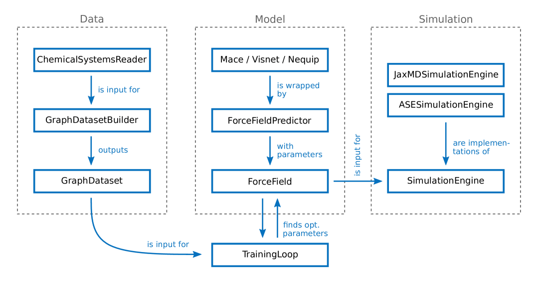
Figure 1: Schematic overview of the essential classes of the mlip library and their interactions. To run simulations with one of the two implementations of SimulationEngine, we need to input an instance of ForceField, which contains a ForceFieldPredictor (implemented as a Flax [53] module) and its parameters. A ForceField instance can be called directly on an input graph. To train the force field model, i.e., find its optimal parameters, we provide a TrainingLoop class that requires training and validation data in GraphDataset objects. These objects can be created easily with tools in the data module. See the tutorials in the code documentation for more details.

3.2 Structure and modules

The mlip library is constructed in a modular way, separating model implementation from training, fine-tuning, and simulation code. It consists of multiple sub-modules targeted towards different parts of a full MLIP pipeline.

1. The data module contains code related to dataset preprocessing. Its main purpose is to go from datasets stored on a file system to instances of GraphDataset classes that can be directly used for training or batched inference tasks.

2. The models module contains code related to the MLIP models, i.e., their core implementations, loss classes, and other related utilities, such as loading of trained models.

3. The training module contains code related to training or fine-tuning MLIP models.

4. The simulation module contains code for running MD simulations or energy minimization with MLIP models. We support both JAX-MD [54] and ASE [55] backends.

5. The inference module contains a function to run batched inference on a list of structures with MLIP models.

6. The utils and typing modules contain utility functions, data classes, and type aliases used in other modules that may also be useful for various downstream tasks.

Each of these modules is designed to allow the user to set up their own experiment scripts or notebooks with minimal effort, while also supporting customization, especially for topics such as logging (e.g. to a remote storage location like Amazon S3 or Google Cloud Storage) or adding new losses, MLIP model architectures, or dataset readers.

In Figure 1, we provide a schematic overview of the most essential classes of the library and how they interact with each other.

3.3 Practical examples

The mlip package can be installed via pip. We provide full code documentation with many tutorials on how to use the library. In the following, we present two common use cases: (1) launching an MD simulation with one of the pre-trained models, and (2) training a model from scratch. These two examples aim to provide a general overview of the library API. For a complete step-by-step walkthrough, please refer to the tutorials.

In the first example, we load a pre-trained MACE model from a zip archive. It is directly loaded into a ForceField object containing all the relevant information about the model. In a subsequent step, we load a chemical system with ASE, initialize the MD config and engine objects, and then launch the run. For more details on logging and results collection, see the deep-dive simulation tutorial provided in the code documentation.

⬇ import ase.io from mlip.models import Mace, ForceField from mlip.models.model_io import ( load_model_from_zip ) from mlip.simulation.jax_md import ( JaxMDSimulationEngine ) # Load pre-trained model force_field = load_model_from_zip( Mace, "/path/to/pretrained_model.zip" ) # Set up MD prerequisites atoms = ase.io.read("/path/to/xyz/or/pdb/file") md_config = JaxMDSimulationEngine.Config( num_steps=1_000_000, # … other settings ) # Run MD md_engine = JaxMDSimulationEngine( atoms, force_field, md_config ) md_engine.run()

• imports: Load the necessary modules. • load_model_from_zip: Loads a pre-trained MACE model from a zip archive into a ForceField object containing all relevant information about the model. Note that the ForceField class can also be viewed as a generic interface for any JAX function that maps jraph.GraphsTuple graphs to our Prediction objects. • ase.io.read: Reads the structure file (as XYZ, PDB, etc.) using ASE. • JaxMDSimulationEngine.Config: Configures the simulation (e.g., number of steps). • JaxMDSimulationEngine: Sets up the molecular dynamics engine. • md_engine.run: Launches the MD simulation.

Although we also provide ASE as a simulation backend, we recommend to rely on the integration with JAX-MD for simulations wherever possible (as in the example above), as it enables running MLIP-based MD with state-of-the-art speed (see benchmarking results of pre-trained models below). With JAX-MD, we can run a collection of multiple MD steps in a fully JIT-compiled manner on the GPU without any data transfer required between CPU and GPU. During this time, any form of logging or saving of intermediate results is not possible. As a consequence, we separate the JAX-MD based simulations into multiple episodes, where logging happens only between two of them.

Furthermore, note that JAX has to recompile the force field prediction function each time its input shapes change, for example, caused by a change in the number of edges resulting from a change in atomic positions. To limit the number of times that JAX must recompile, we apply padding to the neighbor lists and check whether the amount of padding is still sufficient after each episode. If the edge buffer overflowed, we reallocate the neighbor lists and rerun the previous episode. Note that the alternative ASESimulationEngine has an analogous interface to the JaxMDSimulationEngine. With ASE, we also use the same padding strategy to avoid recompiling often. However, reallocation is not limited to happening after episodes but can happen after each MD step if necessary. Therefore, in contrast to the JaxMDSimulationEngine, the ASESimulationEngine will not require a number of episodes to be set in its configuration.

The second example is a code snippet to train a model. We first set up all the prerequisites, which include (1) the dataset (see dedicated data processing tutorial in the documentation for more details), (2) the force field model, (3) the loss, (4) the optimizer, and (5) the training loop config. Once these objects have been set up, one can easily instantiate the training loop class and start the training run. Note that we support multi-GPU training via data parallelism. For more details, see the model training tutorial in the code documentation.

⬇ from mlip.training import ( TrainingLoop, get_default_mlip_optimizer ) from mlip.models.loss import MSELoss from mlip.models import Mace, ForceField # Get data train_set, validation_set, dataset_info = ( _get_dataset() ) # Initialize model mace = Mace(Mace.Config(), dataset_info) force_field = ( ForceField.from_mlip_network(mace) ) # Other prerequisites loss = MSELoss() optimizer = get_default_mlip_optimizer() config = TrainingLoop.Config( num_epochs=100, … # other settings ) # Create TrainingLoop class training_loop = TrainingLoop( train_dataset=train_set, validation_dataset=validation_set, force_field=force_field, loss=loss, optimizer=optimizer, config=config, ) # Start the model training training_loop.run()

• imports: Load the necessary modules. • _get_dataset: Placeholder function to be replaced by code to load a dataset from the filesystem. See the tutorial on data reading processing for more information. Model hyperparameters directly related to the dataset are stored in a DatasetInfo object. • Mace: Initialize a MACE model from a configuration and a DatasetInfo object. In this example, the default hyperparameters are used. • ForceField.from_mlip_network: Creates the ForceField wrapper class (main interface with training and simulation pipelines) from the MACE network class. • MSELoss: Sets up a loss, in this example, a weighted mean-squared error loss for energy, forces, and stress. In this example, the default weights are used. • get_default_mlip_optimizer: Sets up the default optimizer for MLIP models (see the code documentation for more details on how it is implemented). • TrainingLoop.Config: Configures the training loop. • TrainingLoop: Sets up the model training. • training_loop.run: Launches the model training.

4 Dataset and pre-trained models

In this section, we illustrate the use of the library for large-scale training of MLIP models. To that end, we present a set of three pre-trained models, one for each of the architectures included in the library, which were selected from many training runs. Our aim is to illustrate the usage of the library rather than provide usable models. However, these are nonetheless available under a separate license on InstaDeep’s HuggingFace collection. We describe below the dataset used, the training processes, validation results, and runtime benchmarks.

4.1 Curated SPICE2 Dataset

We currently provide access to three pre-trained models, all trained on a curated second version of the SPICE2 dataset [56, 57]. The SPICE2 dataset was chosen for its diversity, both in chemical and conformational space, comprising approximately two million structures computed with DFT at the $\omega$B97M-D3(BJ)/def2-TZVPPD level of approximation. The dataset is labeled and subdivided into a collection of subsets; details of the training and validation sets per subset are provided in Table 1.

Table 1: Summary of training and validation sets. Data categories in columns correspond to those in SPICE2 [57].

	PubChem	DES370K	Amino acid ligand	Dipeptides
Training set	1,284,419	262,820	140,128	19,699
Validation set	58,336	10,917	7,250	1,250
Average size	36.9	16.6	55.4	44.4
	Monomers	Solvated PubChem	Water	Solvated amino acid
Training set	16,750	12,130	1,000	950
Validation set	1,000	705	0	50
Average size	13.5	92.8	95	55.4

To improve data quality, several pre-processing steps were applied. First, any structure where a hydrogen atom did not have exactly one chemical bond (according to a detection mechanism based on covalent radii with appropriate tolerance: 0.4 Å on top of the sum of covalent radii) was removed, eliminating 42,689 structures, as these are likely to be unphysical. Next, since these pre-trained models are not designed to handle charged systems, an additional 142,647 non-neutral structures (total charge) were excluded, stabilizing training. Finally, inspired by the filtering strategy used in MACE-OFF [44], we applied a force filter to remove structures with either a non-zero total force or unusually high per-atom forces. Specifically, we excluded structures with a total force norm exceeding 0.1 eV/Å or any individual force greater than 15 eV/Å. Although this filtering represents a tradeoff, improving force prediction accuracy while slightly reducing energy prediction accuracy on the validation set, it led to improved performance on key benchmarks and was therefore adopted. This step removed an additional 1,024 structures.

4.2 Model training methodology

For the model training, this dataset was then split into training and validation sets using a 95:5 ratio. The split was performed at the molecular SMILES level, ensuring that different conformers of the same molecule were not included in both sets. As a result, some elements which are rare in this curated version of SPICE2 appear only in the training set but not in the validation set (specifically $\mathrm{K}$, $\mathrm{Li}$ and $\mathrm{Na}$). Although this limitation will be addressed in future updates to these MLIP models, users are currently advised to use caution when applying the models to systems containing these elements. The final training set contains 1,737,896 structures covering 15 chemical elements ($\mathrm{B}$, $\mathrm{Br}$, $\mathrm{C}$, $\mathrm{Cl}$, $\mathrm{F}$, $\mathrm{H}$, $\mathrm{I}$, $\mathrm{K}$, $\mathrm{Li}$, $\mathrm{N}$, $\mathrm{Na}$, $\mathrm{O}$, $\mathrm{P}$, $\mathrm{S}$, $\mathrm{Si}$), while the validation set contains 87,922 structures across 12 elements.

Each pre-trained model was trained for 220 epochs using NVIDIA H100 GPUs. The Visnet and NequIP models were trained using the Huber loss [58], while the MACE model used the MSE loss. We have detailed below the key parameters, though full details of the model architectures and training hyperparameters can be found in Appendix A.

• MACE [43, 44, 4, 45]: The MACE pre-trained model hyperparameters were chosen to prioritize stability of MD simulations. The model has 2 layers and 128 channels. The many-body correlation order $\mathrm{correlation}=2$ and the degree of node features $\mathrm{node\leavevmode\nobreak\ symmetry}=3$ (called $\mathrm{max\leavevmode\nobreak\ L}$ in [44]).

• ViSNet [35, 36]: The ViSNet pre-trained model has 4 hidden layers and 128 embedding channels. 8 attention heads were used, as well as 32 RBF features and $L_{\mathrm{max}}=2$.

• NequIP [23]: The NequIP pre-trained model uses 5 interaction blocks and $L_{\mathrm{max}}=2$. The feature configuration is $64\mathrm{x}0\mathrm{e}+64\mathrm{x}0\mathrm{o}+32\mathrm{x}1\mathrm{e}+32\mathrm{x}1\mathrm{o}+4\mathrm{x}2\mathrm{e}+4\mathrm{x}2\mathrm{o}$.

These selected settings on MACE notably differ from those used for MACE-OFF medium [44]. This is because we found that, when training on SPICE2, our updated hyperparameters resulted in significantly better MD stability. To provide comparable models trained on the same dataset, we decided to include this version instead of the one aligned to MACE-OFF, despite the additional computational cost and higher energy prediction errors. We present below validation metrics for both MACE (large - our hyperparameters) and MACE (medium - following the MACE-OFF [44] hyperparameters) on SPICE2. We also conducted a training of MACE aligned to the hyperparameters of MACE-OFF on a curated version of SPICE1 [59]. We found excellent MD stability and validation metrics (more details are presented in Appendix B).

4.3 Model benchmarking

Validation results:

We evaluate the performance of the three pre-trained models, MACE-large, NequIP and VisNet, as well as the MACE-medium model (with hyperparameters aligned to MACE-OFF medium in [44]), on the SPICE2 validation set used during training. Each model was assessed with two standard error metrics: the root mean square error (RMSE) in predicted energies per atom (meV/atom) and the RMSE in atomic forces (meV/Å). Validation was conducted across seven subsets of SPICE2, including isolated and solvated small molecules, as described in Table 1.

Figure 2: Validation set root mean square errors (RMSE) for energy per atom (meV/atom) and atomic forces (meV/Å) across seven molecular subsets in the SPICE2 dataset. The three pretrained models— MACE-large, VisNet, and NequIP— as well as MACE-medium (following the MACE-OFF [44] hyperparameters) are evaluated. The subsets include: PubChem, DES370K, amino acid ligands, dipeptides, monomers, solvated PubChem, and solvated amino acids. RMSE values reflect the deviation from DFT reference calculations. The number of structures per subset is detailed in Table 1.

Figure 2 presents a comparative summary of model performance across all subsets. NequIP achieves the lowest energy RMSE for all subsets, while Visnet outperforms in force RMSE. Across most models, lower force errors are observed in the DES370K, dipeptides, monomers and solvated amino acids subsets than in the PubChem and solvated PubChem subsets. While MACE-medium achieves lower energy RMSE than MACE-large in every subset, MACE-large, on average, outperforms MACE-medium in force RMSE. Users should be warned that while validation errors are relevant metrics to measure training performance, they are not sufficient to attest to a model’s ability to simulate correct physics.

Runtime benchmark:

Conducting a reliable runtime benchmark can be quite challenging. A first obvious reason is the notable difference in implementation across JAX and Torch versions. As a result, we want to point out that the model implementations on which the Torch + ASE benchmarks are run are our own, and they should not be considered representative of the performance of the code developed by the original authors.

(a) 1UAO

(b) 1ABT

Figure 3: Cartoon representations of benchmark systems: (a) chignolin (PDBid: 1UAO) and the alpha-bungarotoxin in complex with a functionally important region of the nicotin acetylcholine receptor (highlighted in grey)

With this in mind, we present in Table 2 simulation benchmarks on two different systems (1UAO and 1ABT, see Figure 3) with results averaged over a 1 nanosecond simulation:

• 1UAO: Chignolin (PDBid: 1UAO) is a synthetic mini-protein, designed to mimic the $\beta$-hairpin secondary structure motif found in natural proteins. Due to its size, Chignolin is widely used in classical molecular dynamics simulations to study folding.

1ABT: Alpha-bungarotoxin complex (PDB: 1ABT, Solution NMR structure) is a potent neurotoxin found in the venom of the Taiwanese many-banded krait snake, Bungarus multicinctus. This small polypeptide (78 amino acids) acts as a highly specific and irreversible antagonist of the nicotinic acetylcholine receptors (nAChRs) at the neuromuscular junction, blocking acetylcholine binding and leading to muscle paralysis. The solved structure displayed in Figure 3 contains alpha-bungarotoxin (BGTX), and a synthetic dodecapeptide (alpha 185-196) corresponding to a functionally important region on the alpha-subunit of the nicotinic acetylcholine receptor (nAChR).

Another important point to note with regard to simulation benchmarks is the significant difference regarding how the JAX + JAX-MD workflow manages GPU utilization and memory compared to the Torch + ASE combination. Simulations on smaller systems will likely exhibit a larger advantage on the JAX versions as it maximizes GPU utilization, unlike the Torch + ASE versions. The relative difference should shrink with increasing system size as GPU capacity gets saturated.

Table 2: Speed performance on MD simulation of the different pre-trained models and backends. All tests were run on a single NVIDIA H100 GPU, and speed metrics are given in milliseconds per step, averaged over 1 ns of simulation. 1UAO is a chignolin molecule with 138 atoms, while 1ABT is a system with 1205 atoms. All models included in the table achieved stable simulations on these benchmarks.

Models	Parameters	Systems	Jax + JAX-MD	Jax + ASE	Torch + ASE
MACE (large)	2,139,152	1UAO	6.3 ms/step	11.6 ms/step	44.2 ms/step
		1ABT	66.8 ms/step	99.5 ms/step	157.2 ms/step
ViSNet	1,137,922	1UAO	2.9 ms/step	6.2 ms/step	33.8 ms/step
		1ABT	25.4 ms/step	46.4 ms/step	101.6 ms/step
NequIP	1,327,792	1UAO	3.8 ms/step	8.5 ms/step	38.7 ms/step
		1ABT	67.0 ms/step	105.7 ms/step	117.0 ms/step

5 Roadmap for library development

We aim to release several updates to the current version (v0.1.0) in the coming months. These will include:

• Ability to incorporate total charge as input and models designed to predict charge-related labels (e.g. partial charges, dipole).

Additional MLIP models with a priority to models that have received validation through additional research. Examples may include eSEN [51] or GemNet [60]. • Accelerated backends for faster inference on steerable convolutions models (e.g. cuEquivariance, sparse kernel generators [61]). • Additional functionalities (e.g. new loss functions, optimizers, layers for MACE, NequIP, or ViSNet). • Release complementary libraries in which mlip will be integrated for additional functionalities (e.g. coarse-grained methods for MLIP [62], or BoostMD [63]). • Training MLIP models on improved and more extensive datasets, for example, the Open Molecules 2025 (OMol25) dataset [5]. Our objective is for any addition to the library to remain open source.

6 Acknowledgements

We would like to acknowledge beta testers for this library: Isabel Wilkinson, Nick Venanzi, Hassan Sirelkhatim, Leon Wehrhan, Sebastien Boyer, Massimo Bortone, Scott Cameron, Louis Robinson, Tom Barrett, and Alex Laterre.

Appendix A Appendix A - Complete set of model and training hyperparameters

A complete description of each parameter can be found in the mlip model documentation. The models were trained using very similar training strategies. Training was performed over 220 epochs with scheduled weights: energy (40) and forces (1000), flipped at epoch 115. An exponential moving average (EMA) with decay rate 0.99 was applied. The AMSGrad variant of Adam optimizer was used. The exponential moving average of the weights is taken at every training step. We use 4000 warmup steps followed by 360000 transition steps. Gradient clipping was performed with a norm of 500, and no gradient accumulation was applied. The ViSNet and NequIP model training was performed using a Huber loss, while the MACE model training was performed using the MSE loss. See Table 3 for the hyperparameters used for the NequIP model, Table 4 for ViSNet, and Table 5 for MACE. All training was done on NVIDIA H100 GPUs. Training took approximately 245 hours for NequIP, 158 hours for ViSNet and 266 hours for MACE.

Table 3: NequIP model hyperparameters.

Parameter	Value
num_layers	5
node_irreps	64x0e + 64x0o + 32x1e + 32x1o + 4x2e + 4x2o
l_max	2
num_bessel	8
radial_net_nonlinearity	swish
radial_net_n_hidden	64
radial_net_n_layers	2
radial_envelope	polynomial_envelope
scalar_mlp_std	4
graph_cutoff_angstrom	5
max_n_node	32
max_n_edge	288
batch_size	16
learning_rate	0.002

Table 4: ViSNet model hyperparameters.

Parameter	Value
num_layers	4
num_channels	128
l_max	2
num_heads	8
num_rbf	32
trainable_rbf	False
activation	silu
attn_activation	silu
vecnorm_type	None
graph_cutoff_angstrom	5
max_n_node	32
max_n_edge	288
batch_size	16
learning_rate	0.0001

Table 5: MACE model hyperparameters.

Parameter	Value
num_layers	2
num_channels	128
l_max	3
node_symmetry	3
correlation	2
readout_irreps	["16x0e","0e"]
num_readout_heads	1
num_bessel	8
activation	silu
radial_envelope	polynomial_envelope
graph_cutoff_angstrom	5
max_n_node	32
max_n_edge	288
batch_size	64
learning_rate	0.01

Appendix B Appendix B - SPICE1 training of MACE medium

As discussed in the main body of the paper, we also trained a version of the MACE architecture of the library on a curated version of SPICE1 [59] with the same parameters as the original MACE-OFF medium model [44]. Overall, we achieved validation performance equivalent to MACE-OFF on SPICE1. We also present in Table 6 the runtime metrics on 1UAO and 1ABT. Likewise, the implementation of the ASE wrapper around the original torch version of MACE-OFF is our own, and it should not be considered representative of the performance of the original authors’ code.

Table 6: Speed performance on MD simulation of the MACE medium pre-trained models and backends. All tests were run on a single NVIDIA H100 GPU and speed metrics are given as milliseconds per step averaged over 1 ns of simulation. 1UAO is a chignolin molecule with 138 atoms, while 1ABT is a system with 1205 atoms. Both models achieved stable simulation, and are both trained on a curated version of SPICE1 [59].

Models	Parameters	Systems	Jax + JAX-MD	Jax + ASE	Torch + ASE
MACE (medium)	1,911,568	1UAO	3.6 ms/step	7.9 ms/step	30.7 ms/step
		1ABT	31.0 ms/step	64.6 ms/step	104.9 ms/step

References

- Stevens et al. [2023] Jan A. Stevens, Fabian Grünewald, P. A. Marco van Tilburg, Melanie König, Benjamin R. Gilbert, Troy A. Brier, Zane R. Thornburg, Zaida Luthey-Schulten, and Siewert J. Marrink. Molecular dynamics simulation of an entire cell. Frontiers in Chemistry, 11, January 2023. 10.3389/fchem.2023.1106495. URL https://doi.org/10.3389/fchem.2023.1106495. Section: Theoretical and Computational Chemistry; Research Topic: Recent Advances in Computational Modelling of Biomolecular Complexes.
- Shaw et al. [2021] David E. Shaw, Peter J. Adams, Asaph Azaria, Joseph A. Bank, Brannon Batson, Alistair Bell, Michael Bergdorf, Jhanvi Bhatt, J. Adam Butts, Timothy Correia, and et al. Anton 3: Twenty microseconds of molecular dynamics simulation before lunch. In Proceedings of the International Conference for High Performance Computing, Networking, Storage and Analysis (SC ’21), New York, NY, USA, 2021. Association for Computing Machinery. 10.1145/3458817.3487397. URL https://doi.org/10.1145/3458817.3487397.
- Bradbury et al. [2018] James Bradbury, Roy Frostig, Peter Hawkins, Matthew J. Johnson, Chris Leary, Dougal Maclaurin, …, and Qiao Zhang. Jax: composable transformations of python+numpy programs. In Proceedings of the 31st Conference on Neural Information Processing Systems (NeurIPS 2018), 2018. URL https://github.com/google/jax.
- Batatia et al. [2024] Ilyes Batatia, Philipp Benner, Yuan Chiang, Alin M. Elena, Dávid P. Kovács, Janosh Riebesell, Xavier R. Advincula, Mark Asta, Matthew Avaylon, William J. Baldwin, Fabian Berger, Noam Bernstein, Arghya Bhowmik, Samuel M. Blau, Vlad Cărare, James P. Darby, Sandip De, Flaviano Della Pia, Volker L. Deringer, Rokas Elijošius, Zakariya El-Machachi, Fabio Falcioni, Edvin Fako, Andrea C. Ferrari, Annalena Genreith-Schriever, Janine George, Rhys E. A. Goodall, Clare P. Grey, Petr Grigorev, Shuang Han, Will Handley, Hendrik H. Heenen, Kersti Hermansson, Christian Holm, Jad Jaafar, Stephan Hofmann, Konstantin S. Jakob, Hyunwook Jung, Venkat Kapil, Aaron D. Kaplan, Nima Karimitari, James R. Kermode, Namu Kroupa, Jolla Kullgren, Matthew C. Kuner, Domantas Kuryla, Guoda Liepuoniute, Johannes T. Margraf, Ioan-Bogdan Magdău, Angelos Michaelides, J. Harry Moore, Aakash A. Naik, Samuel P. Niblett, Sam Walton Norwood, Niamh O’Neill, Christoph Ortner, Kristin A. Persson, Karsten Reuter, Andrew S. Rosen, Lars L. Schaaf, Christoph Schran, Benjamin X. Shi, Eric Sivonxay, Tamás K. Stenczel, Viktor Svahn, Christopher Sutton, Thomas D. Swinburne, Jules Tilly, Cas van der Oord, Eszter Varga-Umbrich, Tejs Vegge, Martin Vondrák, Yangshuai Wang, William C. Witt, Fabian Zills, and Gábor Csányi. A foundation model for atomistic materials chemistry, 2024. URL https://arxiv.org/abs/2401.00096.
- Levine et al. [2025] Daniel S. Levine, Muhammed Shuaibi, Evan Walter Clark Spotte-Smith, Michael G. Taylor, Muhammad R. Hasyim, Kyle Michel, Ilyes Batatia, Gábor Csányi, Misko Dzamba, Peter Eastman, Nathan C. Frey, Xiang Fu, Vahe Gharakhanyan, Aditi S. Krishnapriyan, Joshua A. Rackers, Sanjeev Raja, Ammar Rizvi, Andrew S. Rosen, Zachary Ulissi, Santiago Vargas, C. Lawrence Zitnick, Samuel M. Blau, and Brandon M. Wood. The open molecules 2025 (omol25) dataset, evaluations, and models, 2025. URL https://arxiv.org/abs/2505.08762.
- Bartók et al. [2010] Albert P. Bartók, Mike C. Payne, Risi Kondor, and Gábor Csányi. Gaussian approximation potentials: The accuracy of quantum mechanics, without the electrons. Physical Review Letters, 104(13), April 2010. ISSN 1079-7114. 10.1103/physrevlett.104.136403. URL http://dx.doi.org/10.1103/PhysRevLett.104.136403.
- Bartók and Csányi [2020] Albert P. Bartók and Gábor Csányi. Gaussian approximation potentials: a brief tutorial introduction, 2020. URL https://arxiv.org/abs/1502.01366.
- Bartók et al. [2018] Albert P. Bartók, James Kermode, Noam Bernstein, and Gábor Csányi. Machine learning a general-purpose interatomic potential for silicon. Physical Review X, 8(4), December 2018. ISSN 2160-3308. 10.1103/physrevx.8.041048. URL http://dx.doi.org/10.1103/PhysRevX.8.041048.
- Bartók et al. [2013] Albert P. Bartók, Risi Kondor, and Gábor Csányi. On representing chemical environments. Physical Review B, 87(18), May 2013. ISSN 1550-235X. 10.1103/physrevb.87.184115. URL http://dx.doi.org/10.1103/PhysRevB.87.184115.
- Behler and Parrinello [2007] Jörg Behler and Michele Parrinello. Generalized neural-network representation of high-dimensional potential-energy surfaces. Physical Review Letters, 98(14), April 2007. ISSN 1079-7114. 10.1103/physrevlett.98.146401. URL http://dx.doi.org/10.1103/PhysRevLett.98.146401.
- Thompson et al. [2015] A.P. Thompson, L.P. Swiler, C.R. Trott, S.M. Foiles, and G.J. Tucker. Spectral neighbor analysis method for automated generation of quantum-accurate interatomic potentials. Journal of Computational Physics, 285:316–330, March 2015. ISSN 0021-9991. 10.1016/j.jcp.2014.12.018. URL http://dx.doi.org/10.1016/j.jcp.2014.12.018.
- Chmiela et al. [2017] Stefan Chmiela, Alexandre Tkatchenko, Huziel E. Sauceda, Igor Poltavsky, Kristof T. Schütt, and Klaus-Robert Müller. Machine learning of accurate energy-conserving molecular force fields. Science Advances, 3(5):e1603015, 2017. 10.1126/sciadv.1603015.
- Chmiela et al. [2018] Stefan Chmiela, Huziel E. Sauceda, Klaus-Robert Müller, and Alexandre Tkatchenko. Towards exact molecular dynamics simulations with machine-learned force fields. Nature Communications, 9(1):3887, 2018. 10.1038/s41467-018-06169-2.
- Chmiela et al. [2020] Stefan Chmiela, Huziel E. Sauceda, Alexandre Tkatchenko, and Klaus-Robert Müller. Accurate molecular dynamics enabled by efficient physically-constrained machine learning approaches, pages 129–154. Springer International Publishing, 2020. 10.1007/978-3-030-40245-7_7.
- Chmiela et al. [2023] Stefan Chmiela, Valentin Vassilev-Galindo, Oliver T. Unke, Adil Kabylda, Huziel E. Sauceda, Alexandre Tkatchenko, and Klaus-Robert Müller. Accurate global machine learning force fields for molecules with hundreds of atoms. Science Advances, 9(2):eadf0873, 2023. 10.1126/sciadv.adf0873.
- Drautz [2019] Ralf Drautz. Atomic cluster expansion for accurate and transferable interatomic potentials. Physical Review B, 99(1), January 2019. ISSN 2469-9969. 10.1103/physrevb.99.014104. URL http://dx.doi.org/10.1103/PhysRevB.99.014104.
- Shapeev [2016] Alexander V. Shapeev. Moment tensor potentials: A class of systematically improvable interatomic potentials. Multiscale Modeling & Simulation, 14(3):1153–1173, January 2016. ISSN 1540-3467. 10.1137/15m1054183. URL http://dx.doi.org/10.1137/15M1054183.
- Smith et al. [2017] J. S. Smith, O. Isayev, and A. E. Roitberg. Ani-1: an extensible neural network potential with dft accuracy at force field computational cost. Chemical Science, 8(4):3192–3203, 2017. ISSN 2041-6539. 10.1039/c6sc05720a. URL http://dx.doi.org/10.1039/C6SC05720A.
- Smith et al. [2020] Justin S. Smith, Roman Zubatyuk, Benjamin Nebgen, Nicholas Lubbers, Kipton Barros, Adrian E. Roitberg, Olexandr Isayev, and Sergei Tretiak. The ani-1ccx and ani-1x data sets, coupled-cluster and density functional theory properties for molecules. Scientific Data, 7(1), May 2020. ISSN 2052-4463. 10.1038/s41597-020-0473-z. URL http://dx.doi.org/10.1038/s41597-020-0473-z.
- Smith et al. [2019] Justin S. Smith, Benjamin T. Nebgen, Roman Zubatyuk, Nicholas Lubbers, Christian Devereux, Kipton Barros, Sergei Tretiak, Olexandr Isayev, and Adrian E. Roitberg. Approaching coupled cluster accuracy with a general-purpose neural network potential through transfer learning. Nature Communications, 10(1), July 2019. ISSN 2041-1723. 10.1038/s41467-019-10827-4. URL http://dx.doi.org/10.1038/s41467-019-10827-4.
- Devereux et al. [2020] Christian Devereux, Justin S. Smith, Kate K. Huddleston, Kipton Barros, Roman Zubatyuk, Olexandr Isayev, and Adrian E. Roitberg. Extending the applicability of the ani deep learning molecular potential to sulfur and halogens. Journal of Chemical Theory and Computation, 16(7):4192–4202, June 2020. ISSN 1549-9626. 10.1021/acs.jctc.0c00121. URL http://dx.doi.org/10.1021/acs.jctc.0c00121.
- Rezaee et al. [2024] Mozafar Rezaee, Saeid Ekrami, and Seyed Majid Hashemianzadeh. Comparing ani-2x, ani-1ccx neural networks, force field, and dft methods for predicting conformational potential energy of organic molecules. Scientific Reports, 14(1), May 2024. ISSN 2045-2322. 10.1038/s41598-024-62242-5. URL http://dx.doi.org/10.1038/s41598-024-62242-5.
- Batzner et al. [2022] Simon Batzner, Albert Musaelian, Lixin Sun, Mario Geiger, Jonathan P. Mailoa, Mordechai Kornbluth, Nicola Molinari, Tess E. Smidt, and Boris Kozinsky. E(3)-equivariant graph neural networks for data-efficient and accurate interatomic potentials. Nature Communications, 13(1), May 2022. ISSN 2041-1723. 10.1038/s41467-022-29939-5. URL http://dx.doi.org/10.1038/s41467-022-29939-5.
- Brehmer et al. [2024] Johann Brehmer, Sönke Behrends, Pim de Haan, and Taco Cohen. Does equivariance matter at scale?, 2024. URL https://arxiv.org/abs/2410.23179.
- Schütt et al. [2018] K. T. Schütt, H. E. Sauceda, P.-J. Kindermans, A. Tkatchenko, and K.-R. Müller. Schnet – a deep learning architecture for molecules and materials. The Journal of Chemical Physics, 148(24), March 2018. ISSN 1089-7690. 10.1063/1.5019779. URL http://dx.doi.org/10.1063/1.5019779.
- Schütt et al. [2019] Kristof T. Schütt, Pan Kessel, Michael Gastegger, Kim A. Nicoli, Alexandre Tkatchenko, and Klaus-Robert Müller. SchNetPack: A Deep Learning Toolbox For Atomistic Systems. Journal of Chemical Theory and Computation, 15(1):448–455, 2019. 10.1021/acs.jctc.8b00908. URL https://doi.org/10.1021/acs.jctc.8b00908.
- Schütt et al. [2023] Kristof T. Schütt, Stefaan S. P. Hessmann, Niklas W. A. Gebauer, Jonas Lederer, and Michael Gastegger. SchNetPack 2.0: A neural network toolbox for atomistic machine learning. The Journal of Chemical Physics, 158(14):144801, 04 2023. ISSN 0021-9606. 10.1063/5.0138367. URL https://doi.org/10.1063/5.0138367.
- Xie and Grossman [2018] Tian Xie and Jeffrey C. Grossman. Crystal graph convolutional neural networks for an accurate and interpretable prediction of material properties. Physical Review Letters, 120(14), April 2018. ISSN 1079-7114. 10.1103/physrevlett.120.145301. URL http://dx.doi.org/10.1103/PhysRevLett.120.145301.
- Anstine et al. [2025] Dylan M. Anstine, Roman Zubatyuk, and Olexandr Isayev. Aimnet2: a neural network potential to meet your neutral, charged, organic, and elemental-organic needs. Chemical Science, 2025. ISSN 2041-6539. 10.1039/d4sc08572h. URL http://dx.doi.org/10.1039/D4SC08572H.
- Satorras et al. [2022] Victor Garcia Satorras, Emiel Hoogeboom, and Max Welling. E(n) equivariant graph neural networks, 2022. URL https://arxiv.org/abs/2102.09844.
- Gasteiger et al. [2020a] Johannes Gasteiger, Janek Groß, and Stephan Günnemann. Directional message passing for molecular graphs. In International Conference on Learning Representations (ICLR), 2020a.
- Gasteiger et al. [2020b] Johannes Gasteiger, Shankari Giri, Johannes T. Margraf, and Stephan Günnemann. Fast and uncertainty-aware directional message passing for non-equilibrium molecules. In Machine Learning for Molecules Workshop, NeurIPS, 2020b.
- Gasteiger et al. [2021] Johannes Gasteiger, Florian Becker, and Stephan Günnemann. Gemnet: Universal directional graph neural networks for molecules. In M. Ranzato, A. Beygelzimer, Y. Dauphin, P.S. Liang, and J. Wortman Vaughan, editors, Advances in Neural Information Processing Systems, volume 34, pages 6790–6802. Curran Associates, Inc., 2021. URL https://proceedings.neurips.cc/paper_files/paper/2021/file/35cf8659cfcb13224cbd47863a34fc58-Paper.pdf.
- Gasteiger et al. [2024] Johannes Gasteiger, Florian Becker, and Stephan Günnemann. Gemnet: Universal directional graph neural networks for molecules, 2024. URL https://arxiv.org/abs/2106.08903.
- Wang et al. [2024a] Yusong Wang, Tong Wang, Shaoning Li, Xinheng He, Mingyu Li, Zun Wang, Nanning Zheng, Bin Shao, and Tie-Yan Liu. Enhancing geometric representations for molecules with equivariant vector-scalar interactive message passing. Nature Communications, 15(1), January 2024a. ISSN 2041-1723. 10.1038/s41467-023-43720-2. URL http://dx.doi.org/10.1038/s41467-023-43720-2.
- Wang et al. [2024b] Tong Wang, Xinheng He, Mingyu Li, Yatao Li, Ran Bi, Yusong Wang, Chaoran Cheng, Xiangzhen Shen, Jiawei Meng, He Zhang, Haiguang Liu, Zun Wang, Shaoning Li, Bin Shao, and Tie-Yan Liu. Ab initio characterization of protein molecular dynamics with ai2bmd. Nature, 635(8040):1019–1027, November 2024b. ISSN 1476-4687. 10.1038/s41586-024-08127-z. URL http://dx.doi.org/10.1038/s41586-024-08127-z.
- Weiler et al. [2018] Maurice Weiler, Mario Geiger, Max Welling, Wouter Boomsma, and Taco Cohen. 3d steerable cnns: Learning rotationally equivariant features in volumetric data, 2018. URL https://arxiv.org/abs/1807.02547.
- Kondor et al. [2018] Risi Kondor, Zhen Lin, and Shubhendu Trivedi. Clebsch-gordan nets: a fully fourier space spherical convolutional neural network, 2018. URL https://arxiv.org/abs/1806.09231.
- Batatia et al. [2022] Ilyes Batatia, Simon Batzner, Dávid Péter Kovács, Albert Musaelian, Gregor N. C. Simm, Ralf Drautz, Christoph Ortner, Boris Kozinsky, and Gábor Csányi. The design space of e(3)-equivariant atom-centered interatomic potentials, 2022. URL https://arxiv.org/abs/2205.06643.
- Thomas et al. [2018] Nathaniel Thomas, Tess Smidt, Steven Kearnes, Lusann Yang, Li Li, Kai Kohlhoff, and Patrick Riley. Tensor field networks: Rotation- and translation-equivariant neural networks for 3d point clouds, 2018. URL https://arxiv.org/abs/1802.08219.
- Musaelian et al. [2023a] Albert Musaelian, Simon Batzner, Anders Johansson, Lixin Sun, Cameron J. Owen, Mordechai Kornbluth, and Boris Kozinsky. Learning local equivariant representations for large-scale atomistic dynamics. Nature Communications, 14(1), February 2023a. ISSN 2041-1723. 10.1038/s41467-023-36329-y. URL http://dx.doi.org/10.1038/s41467-023-36329-y.
- Musaelian et al. [2023b] Albert Musaelian, Anders Johansson, Simon Batzner, and Boris Kozinsky. Scaling the leading accuracy of deep equivariant models to biomolecular simulations of realistic size, 2023b. URL https://arxiv.org/abs/2304.10061.
- Batatia et al. [2023] Ilyes Batatia, Dávid Péter Kovács, Gregor N. C. Simm, Christoph Ortner, and Gábor Csányi. Mace: Higher order equivariant message passing neural networks for fast and accurate force fields, 2023. URL https://arxiv.org/abs/2206.07697.
- Kovács et al. [2025] Dávid Péter Kovács, J. Harry Moore, Nicholas J. Browning, Ilyes Batatia, Joshua T. Horton, Yixuan Pu, Venkat Kapil, William C. Witt, Ioan-Bogdan Magdău, Daniel J. Cole, and Gábor Csányi. Mace-off: Short-range transferable machine learning force fields for organic molecules. Journal of the American Chemical Society, May 2025. ISSN 1520-5126. 10.1021/jacs.4c07099. URL http://dx.doi.org/10.1021/jacs.4c07099.
- Kovács et al. [2023] Dávid Péter Kovács, Ilyes Batatia, Eszter Sára Arany, and Gábor Csányi. Evaluation of the mace force field architecture: From medicinal chemistry to materials science. The Journal of Chemical Physics, 159(4), July 2023. ISSN 1089-7690. 10.1063/5.0155322. URL http://dx.doi.org/10.1063/5.0155322.
- Schütt et al. [2021] Kristof T. Schütt, Oliver T. Unke, and Michael Gastegger. Equivariant message passing for the prediction of tensorial properties and molecular spectra, 2021. URL https://arxiv.org/abs/2102.03150.
- Geiger et al. [2022] Mario Geiger, Tess Smidt, Alby M., Benjamin Kurt Miller, Wouter Boomsma, Bradley Dice, Kostiantyn Lapchevskyi, Maurice Weiler, Michał Tyszkiewicz, Simon Batzner, Dylan Madisetti, Martin Uhrin, Jes Frellsen, Nuri Jung, Sophia Sanborn, Mingjian Wen, Josh Rackers, Marcel Rød, and Michael Bailey. Euclidean neural networks: e3nn, April 2022. URL https://doi.org/10.5281/zenodo.6459381.
- Unke and Maennel [2024] Oliver T. Unke and Hartmut Maennel. E3x: -equivariant deep learning made easy. arXiv preprint arXiv:2401.07595, 2024.
- Passaro and Zitnick [2023] Saro Passaro and C. Lawrence Zitnick. Reducing so(3) convolutions to so(2) for efficient equivariant gnns. In Proceedings of the 40th International Conference on Machine Learning, ICML’23. JMLR.org, 2023.
- Luo et al. [2024] Shengjie Luo, Tianlang Chen, and Aditi S. Krishnapriyan. Enabling efficient equivariant operations in the fourier basis via gaunt tensor products, 2024. URL https://arxiv.org/abs/2401.10216.
- Fu et al. [2025] Xiang Fu, Brandon M. Wood, Luis Barroso-Luque, Daniel S. Levine, Meng Gao, Misko Dzamba, and C. Lawrence Zitnick. Learning smooth and expressive interatomic potentials for physical property prediction, 2025. URL https://arxiv.org/abs/2502.12147.
- Merchant et al. [2023] Amil Merchant, Simon Batzner, Samuel S. Schoenholz, Muratahan Aykol, Gowoon Cheon, and Ekin Dogus Cubuk. Scaling deep learning for materials discovery. Nature, 2023. 10.1038/s41586-023-06735-9.
- Heek et al. [2024] Jonathan Heek, Anselm Levskaya, Avital Oliver, Marvin Ritter, Bertrand Rondepierre, Andreas Steiner, and Marc van Zee. Flax: A neural network library and ecosystem for JAX, 2024. URL http://github.com/google/flax.
- Schoenholz and Cubuk [2020] Samuel S. Schoenholz and Ekin D. Cubuk. Jax, m.d.: A framework for differentiable physics, 2020. URL https://arxiv.org/abs/1912.04232.
- Hjorth Larsen et al. [2017] Ask Hjorth Larsen, Jens Jørgen Mortensen, Jakob Blomqvist, Ivano E Castelli, Rune Christensen, Marcin Dułak, Jesper Friis, Michael N Groves, Bjørk Hammer, Cory Hargus, Eric D Hermes, Paul C Jennings, Peter Bjerre Jensen, James Kermode, John R Kitchin, Esben Leonhard Kolsbjerg, Joseph Kubal, Kristen Kaasbjerg, Steen Lysgaard, Jón Bergmann Maronsson, Tristan Maxson, Thomas Olsen, Lars Pastewka, Andrew Peterson, Carsten Rostgaard, Jakob Schiøtz, Ole Schütt, Mikkel Strange, Kristian S Thygesen, Tejs Vegge, Lasse Vilhelmsen, Michael Walter, Zhenhua Zeng, and Karsten W Jacobsen. The atomic simulation environment—a python library for working with atoms. Journal of Physics: Condensed Matter, 29(27):273002, June 2017. ISSN 1361-648X. 10.1088/1361-648x/aa680e. URL http://dx.doi.org/10.1088/1361-648X/aa680e.
- Eastman et al. [2023] Peter Eastman, Pavan Kumar Behara, David L. Dotson, Raimondas Galvelis, John E. Herr, Josh T. Horton, Yuezhi Mao, John D. Chodera, Benjamin P. Pritchard, Yuanqing Wang, Gianni De Fabritiis, and Thomas E. Markland. Spice, a dataset of drug-like molecules and peptides for training machine learning potentials. Scientific Data, 10, January 2023. 10.1038/s41597-022-01882-6. URL https://doi.org/10.1038/s41597-022-01882-6.
- Eastman et al. [2024] Peter Eastman, Benjamin P, Pritchard, John D. Chodera, and Thomas E. Markland. Nutmeg and spice: Models and data for biomolecular machine learning, 2024. URL https://arxiv.org/abs/2406.13112.
- Huber [1992] Peter J. Huber. Robust Estimation of a Location Parameter, pages 492–518. Springer New York, New York, NY, 1992. ISBN 978-1-4612-4380-9. 10.1007/978-1-4612-4380-9_35. URL https://doi.org/10.1007/978-1-4612-4380-9_35.
- Moore et al. [2024] Harry Moore, David Peter Kovacs, Nicholas J Browning, Ilyes Batatia, Joshua T Horton, Venkat Kapil, William Witt, Ioan Magdau, Daniel Cole, and Gabor Csanyi. Research data supporting "mace-off23", 2024. URL https://www.repository.cam.ac.uk/handle/1810/366661.
- Gasteiger et al. [2022] Johannes Gasteiger, Muhammed Shuaibi, Anuroop Sriram, Stephan Günnemann, Zachary Ulissi, C. Lawrence Zitnick, and Abhishek Das. Gemnet-oc: Developing graph neural networks for large and diverse molecular simulation datasets, 2022. URL https://arxiv.org/abs/2204.02782.
- Bharadwaj et al. [2025] Vivek Bharadwaj, Austin Glover, Aydin Buluc, and James Demmel. An efficient sparse kernel generator for o(3)-equivariant deep networks, 2025. URL https://arxiv.org/abs/2501.13986.
- Brunken et al. [2025] Christoph Brunken, Sebastien Boyer, Mustafa Omar, Martin Maarand, Olivier Peltre, Solal Attias, Bakary N’tji Diallo, Anastasia Markina, Olaf Othersen, and Oliver Bent. Universally applicable and tunable graph-based coarse-graining for machine learning force fields, 2025. URL https://arxiv.org/abs/2504.01973.
- Schaaf et al. [2024] Lars L. Schaaf, Ilyes Batatia, Christoph Brunken, Thomas D. Barrett, and Jules Tilly. Boostmd: Accelerating molecular sampling by leveraging ml force field features from previous time-steps, 2024. URL https://arxiv.org/abs/2412.18633.