Configuration-dependent precision in magnetometry and thermometry using multi-qubit quantum sensors

Abstract

We study the performance of quantum sensors composed of four qubits arranged in different geometries for magnetometry and thermometry. The qubits interact via the transverse-field Ising model with both ferromagnetic and antiferromagnetic couplings, maintained in thermal equilibrium with a heat bath under an external magnetic field. Using quantum Fisher information (QFI), we evaluate the metrological precision of these sensors. For ferromagnetic couplings, weakly connected graphs (e.g., the chain graph, $P_{4}$) perform optimally in estimating weak magnetic fields, whereas highly connected graphs (e.g., the complete graph, $K_{4}$) excel at strong fields. Conversely, $K_{4}$ achieves the highest sensitivity for temperature estimation in the weak-field regime. In the antiferromagnetic case, we uncover a fundamental trade-off dictated by spectral degeneracy: configurations with non-degenerate energy spectra—such as the pan-like graph (three qubits in a triangle with the fourth attached)—exhibit strong magnetic field sensitivity due to their pronounced response to perturbations. In contrast, symmetric structures like the square graph, featuring degenerate energy levels (particularly ground-state degeneracy), are better suited for precise thermometry. Notably, our four-qubit sensors achieve peak precision in the low-temperature, weak-field regime. Finally, we introduce a spectral sensitivity measure that quantifies energy spectrum deformations under small perturbations, offering a tool to optimize magnetometric performance.

I Introduction

Quantum metrology leverages quantum properties such as coherence Wang et al. (2018); Cheng et al. (2019); Joo et al. (2011) and entanglement Huang et al. (2016); Joo et al. (2011) to enhance measurement precision Giovannetti et al. (2006); Degen et al. (2017); Tóth and Apellaniz (2014); Giovannetti et al. (2011). Its applications range from biomedical imaging Aslam et al. (2023); Taylor and Bowen (2016) to fundamental physics DeMille et al. (2024), pushing the boundaries of what can be reliably estimated. Temperature is a key physical parameter with broad relevance in physics, chemistry, and biology. Advanced thermal sensing techniques Mehboudi et al. (2019); Dedyulin et al. (2022); Moreva et al. (2020); Wang et al. (2020); Brenes and Segal (2023); Gottscholl et al. (2021), including photonic Klimov et al. (2018); Li et al. (2010); Dong et al. (2009), optomechanical Purdy et al. (2017), and cavity QED-based methods Chowdhury et al. (2019); Singh and Purdy (2020); Galinskiy et al. (2020), have been developed. Quantum approaches, such as critical Aybar et al. (2022); Yu et al. (2024); Salvatori et al. (2014); Zhang et al. (2022a); Mok et al. (2021); Zanardi et al. (2008) and collisional thermometry Seah et al. (2019), as well as those using cold atoms or spins De Daniloff et al. (2021); Glatthard et al. (2022); Roscilde (2014), offer promising advancements. Similarly, quantum-enhanced magnetometry plays a crucial role in detecting weak magnetic fields with high precision Brask et al. (2015); Razzoli et al. (2019); Wasilewski et al. (2010); Troiani and Paris (2018); Troullinou et al. (2023); Montenegro et al. (2022); Razzoli et al. (2019); Shukla and Chandrashekar (2024); Li et al. (2018); Albarelli et al. (2017).

The structure and connectivity of quantum sensors are key to optimizing their performance, much like structured networks in biological and many-body quantum systems Ishizaki and Fleming (2012). Nature exploits connectivity for enhanced functionality, and quantum networks use similar principles for sensing Proctor et al. (2018); Bringewatt et al. (2021) and information processing Gassab et al. (2024); Upadhyay and Marathe (2024). Extending these principles to quantum thermometry, it has been investigated recently Candeloro et al. (2021) how topology influences quantum thermometry precision by modeling the probe as a continuous-time quantum walker (CTQW), with the Hamiltonian corresponding to the graph Laplacian. Those results suggest that small algebraic connectivity is advantageous for precise temperature sensing. In that reference, CTQW is used, which is directly related to the geometry of the spin network connectivity. However, the interplay between the underlying configuration geometry of the spins and the Hamiltonian of spin-spin interactions can be more complex in other models, such as the transverse-field Ising model. This distinction is critical for many applications, including quantum annealers Lechner et al. (2015); Nigg et al. (2017). In our model system, we consider a transverse-field Ising model, and our optimum multi-qubit sensor configurations do not align with the categorizations found for CTQW models in Ref. Candeloro et al. (2021).

Building on these insights—but departing from the single-particle framework—we investigate the structural optimization of quantum sensors for both magnetometry and thermometry. Our quantum sensor is composed of four qubits arranged in six distinct connected graph-like configurations, where both the connectivity and arrangement of qubits play crucial yet subtle roles in sensing performance, as they shape the spectral structure of the network Hamiltonian and, in turn, influence the ultimate precision limits. The qubits interact via the transverse field Ising model, considering both ferromagnetic and antiferromagnetic couplings, and are coupled to a thermal bath under an external weak and uniform magnetic field, with the equilibrium state described by a Gibbs thermal state of the overall Hamiltonian. To quantify precision limits, we employ the quantum Fisher information (QFI), focusing on temperature and magnetic field estimation. We also introduce a spectral sensitivity measure, which captures the deformation of the energy spectrum under small perturbations, as a tool to identify configurations with enhanced quantum sensitivity.

In the ferromagnetic regime, we investigate how the structural configuration of the multi-qubit quantum sensor impacts the precision of parameter estimation. When estimating a weak magnetic field $h$, sensors with minimal connectivity, such as the linear-chain graph ($P_{4}$), demonstrate optimal performance. Their low degree and simple energy spectra with degenerate ground states allow efficient spin flips at low fields, enhancing quantum fluctuations and yielding a large QFI. The star graph ($S_{3}$) similarly performs well due to comparable spectral properties. In contrast, highly connected structures like the complete graph ($K_{4}$) are stiffer, resisting spin flips and thus requiring stronger magnetic fields to achieve significant sensitivity. As a result, graphs with higher connectivity outperform at stronger magnetic fields, although the maximum achievable precision slightly decreases. For temperature estimation, the situation is somewhat different. The optimal performance depends on both the structure and the type of ferromagnetic or antiferromagnetic coupling. The complete graph ($K_{4}$) shows the highest thermal sensitivity, benefiting from its highest connectivity, which balances energy level structure and thermal susceptibility. The connection between the thermal QFI and the heat capacity emphasizes that structures with a spectrum favoring low-energy excitations yield better performance at low temperatures, but stiffer graphs maintain better sensitivity under stronger external fields.

In the antiferromagnetic case, our findings indicate that the optimal configuration for magnetic field estimation is a pan graph (a triangle with a pendant vertex). The precision of magnetic sensing is closely linked to the eigenvalue spectrum of the system’s Hamiltonian. Intuitively, unless special entangled states are used to exploit degeneracies, non-degenerate energy levels generally enhance magnetic sensitivity, whereas degenerate levels limit the system’s ability to distinguish between energy levels under magnetic perturbations. The presence of degeneracies, particularly ground-state degeneracy, in the spectrum reduces the contrast in the system’s response to changes in the magnetic field, thereby diminishing its ability to extract information from magnetic perturbations. Among the considered configurations, the pan graph (and $K_{4}$) exhibits fewer symmetries in the energy spectrum compared to the others, resulting in a highly non-degenerate spectrum, with no ground state degeneracy, which is particularly advantageous for magnetic sensing. Notably, among the 4-qubit sensor configurations, the pan graph possesses a nearly non-degenerate spectrum, making it the most favorable choice for precision magnetometry. In contrast, the $C_{4}$ graph configuration is the most effective for temperature estimation, as its highly symmetric energy spectrum exhibits a near-degenerate ground state in the weak-field regime, and consequently offers the highest sensitivity to temperature variations. This result aligns with existing literature, where it is well established that degeneracy enhances thermal sensitivity Campbell et al. (2018); Correa et al. (2015); Płodzień et al. (2018); Srivastava et al. (2023, 2025). In addition, among the six distinct connected graphs for a four-qubit sensor, the square configuration demonstrates the sharpest Boltzmann factor variation with temperature, enabling rapid state population changes and superior temperature sensitivity compared to more gradual-response alternatives. Notably, the pan and $K_{4}$ graphs are the only configurations that do not have ground state degeneracy, and the energy levels are more shifted under magnetic perturbation, making them good magnetometers. In contrast, the other configurations, with ground state degeneracy, are more effective for temperature sensing, making them better suited as thermometers.

Overall, the sensor’s energy spectrum, connectivity, and degree of symmetry are critical factors in optimizing quantum sensing: sparse graphs offer superior sensitivity for weak-field magnetometry, while more connected graphs provide robustness under strong fields, enhancing both high-field magnetometry and thermometric precision.

The remainder of the paper is structured as follows. In Sec. II, we introduce the fundamental concepts of quantum parameter estimation theory. Sec. III provides an overview of the model used in this study. The results for quantum magnetometry and thermometry are discussed in Sec. IV. In Sec. V we introduce a spectral deformation measure that can identify the sensor configurations with maximum magnetic field sensitivity. We discuss the role of the external magnetic field on the energy spectrum of each configuration in Appendix A and the effect of temperature on the precision of the magnetic field in Appendix B. Finally, Sec. VI concludes with a summary of our findings.

II Parameter estimation theory

In this section, we provide a concise overview of quantum estimation theory, focusing on single-parameter estimation. We introduce key concepts and tools that will be used throughout this study. In quantum metrology, the maximum achievable precision about an unknown parameter $\theta$ is quantified by quantum Fisher information (QFI). For any parameterized quantum state $\rho_{\theta}$ , the ultimate precision limit in estimating the parameter $\theta$ is determined by the Cramér-Rao bound such that the variance of any estimator $\hat{\theta}$ is lower bounded by the reciprocal of the QFI. The mathematical expression is given by Paris (2009); Helstrom (1969a); Sidhu and Kok (2020); Braunstein and Caves (1994); Helstrom (1969b)

$$\text{Var}(\theta)\geq\frac{1}{mF_{Q}(\theta)},$$ (1)

where $\text{Var}(\theta)$ denotes the variance, $m$ represents the number of measurements repeated, which is $m=1$ for a single-shot scenario, and $F_{Q}(\theta)$ is the QFI, which depends on the quantum state $\rho_{\theta}$ and its parameterization process. The QFI is maximized over all possible POVMS Braunstein and Caves (1994) to obtain the ultimate bound on the precision of parameter $\theta$. For a mixed state, the QFI is defined as

$$F_{Q}(\theta)=\text{Tr}[\rho_{\theta}L_{\theta}^{2}],$$ (2)

where $L_{\theta}$ is the symmetric logarithmic derivative (SLD), a Hermitian operator which is explicitly defined by

$$\frac{\partial\rho_{\theta}}{\partial\theta}=\frac{L_{\theta}\rho_{\theta}+\rho_{\theta}L_{\theta}}{2}.$$ (3)

If we express $L_{\theta}$ in the eigenbasis of $\rho_{\theta}$, the QFI can be written as follows:

$$F_{Q}(\theta)=2\sum_{n,m}\frac{|\langle\psi_{n}|\partial_{\theta}\rho_{\theta}|\psi_{m}\rangle|^{2}}{\lambda_{n}+\lambda_{m}},$$ (4)

where $\lambda_{n}$ and $\lambda_{m}$ are the eigenvalues and $|\psi_{n}\rangle$ and $|\psi_{m}\rangle$ represent the eigenvectors of the density matrix $\rho_{\theta}$ and $\partial_{\theta}=\partial/\partial_{\theta}$ is the partial derivative with respect to $\theta$.

We remark that the SLD is defined based on the density matrix $\rho_{\theta}$ and both the eigenvalues $\lambda_{n}$ and eigenvectors $|\psi_{n}\rangle$ may depend on the parameter $\theta$. Therefore, we can separate the contribution of QFI into two parts by using the Leibniz rule:

$$\partial_{\theta}\rho_{\theta} =\sum_{n}\big{(}(\partial_{\theta}\rho_{\theta})|\psi_{n}\rangle\langle\psi_{n}|$$ (5)

$$\quad+\rho_{\theta}|\partial_{\theta}\psi_{n}\rangle\langle\psi_{n}|+\rho_{\theta}|\psi_{n}\rangle\langle\partial_{\theta}\psi_{n}|\big{)},$$

The symbol $|\partial_{\theta}\psi_{n}\rangle$ denotes the ket, such as

$$|\partial_{\theta}\psi_{n}\rangle=\sum_{k}\partial_{\theta}\psi_{nk}|k\rangle,$$ (6)

where $\psi_{nk}$ are obtained by expanding $|\psi_{n}\rangle$ in an arbitrary basis $\{|k\rangle\}$ independent of $\theta$. Since $\langle\psi_{n}|\psi_{m}\rangle=\delta_{nm}$, we have

$$\partial_{\theta}\langle\psi_{n}|\psi_{m}\rangle\equiv\langle\partial_{\theta}\psi_{n}|\psi_{m}\rangle+\langle\psi_{n}|\partial_{\theta}\psi_{m}\rangle=0$$ (7)

and therefore

$$\text{Re}\langle\partial_{\theta}\psi_{n}|\psi_{m}\rangle=0,\quad\langle\partial_{\theta}\psi_{n}|\psi_{m}\rangle=-\langle\psi_{n}|\partial_{\theta}\psi_{m}\rangle=0.$$ (8)

Using Eq. (5) and the above identities, we have

$$L_{\theta} =\sum_{p}\frac{\partial_{\lambda}\lambda_{p}}{\lambda_{p}}|\psi_{p}\rangle\langle\psi_{p}|$$ (9)

$$+2\sum_{n\neq m}\frac{\lambda_{n}-\lambda_{m}}{\lambda_{n}+\lambda_{m}}\langle\psi_{m}|\partial_{\theta}\psi_{n}\rangle|\psi_{m}\rangle\langle\psi_{n}|$$

and in turn, the QFI takes the form

$$F_{Q}(\theta)=\sum_{p}\frac{(\partial_{\theta}\lambda_{p})^{2}}{\lambda_{p}}+2\sum_{n\neq m}\frac{(\lambda_{n}-\lambda_{m})^{2}}{\lambda_{n}+\lambda_{m}}|\langle\psi_{m}|\partial_{\theta}\psi_{n}\rangle|^{2}.$$ (10)

The first term in Eq. (10) represents the classical contribution to the QFI, while the second term captures the purely quantum contribution. In this work, we focus on single-parameter estimation, exploiting the field as an external tuning to possibly enhance thermometry, and temperature as a source of noise in the estimation of the magnetic field. Joint estimation of the two quantities may be investigated further, but it is beyond the scope of this work, and will be addressed elsewhere.

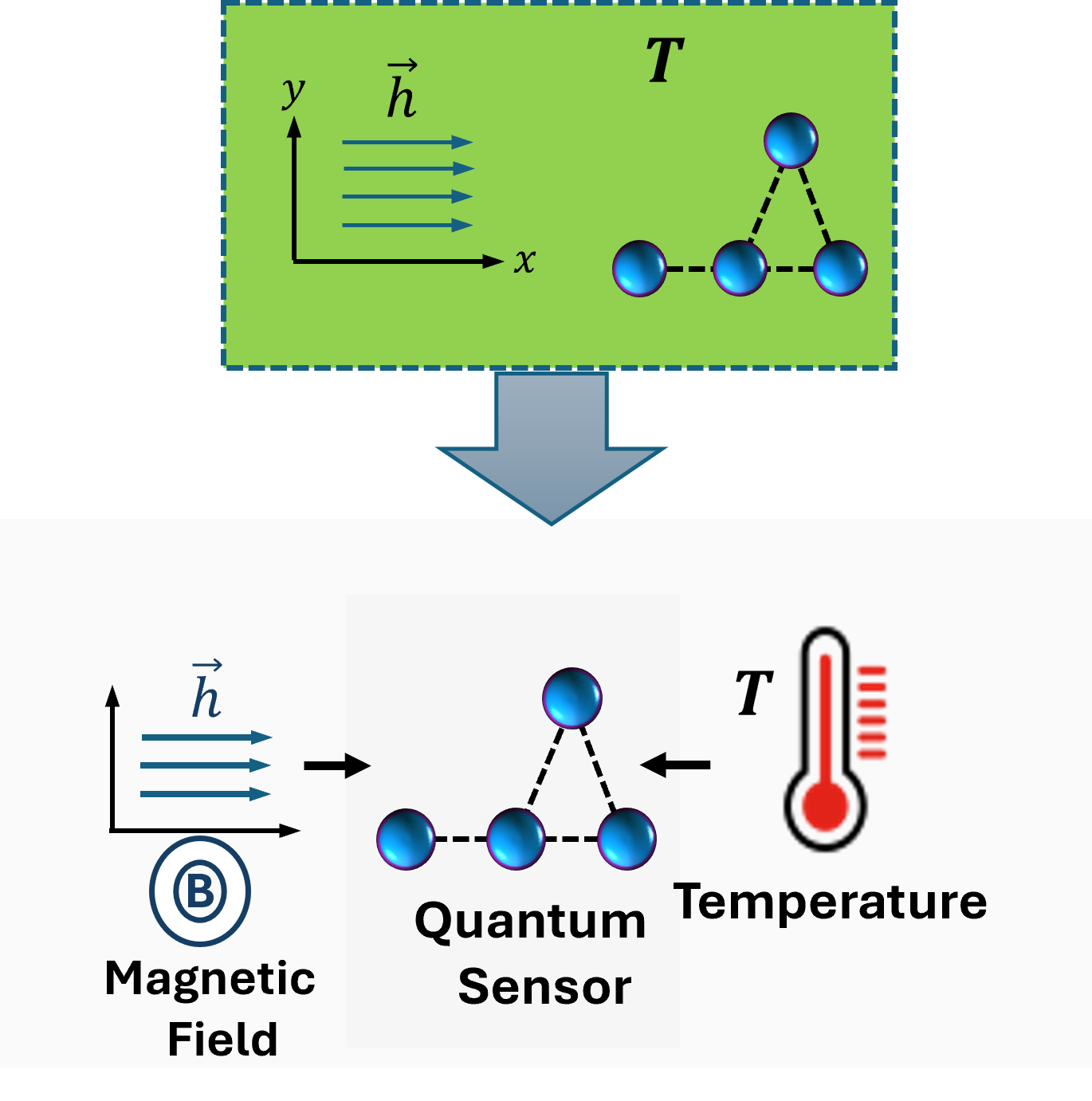
Figure 1: Model representation of our quantum sensing protocol. The quantum sensor, modeled as a network of four coupled spins, simultaneously exposed to a thermal bath at temperature $T$ and an external weak magnetic field with magnitude $\vec{h}$, directed along $x$-axis. The sensor functions as a probe to estimate unknown parameters, including $T$ and $h$. The different configurations of the quantum sensor are given in Fig. 2.

III The Model

In this work, we consider a finite-size quantum sensor consisting of four coupled spin-$1/2$ particles, such as qubits, coupled via an Ising spin chain in the presence of an external magnetic field. We assume that the sensor is in thermal equilibrium with a thermal bath at temperature $T$. The sensor is used to measure both the magnetic field and temperature (see Fig. 1).

The four spins can be arranged in six different configurations, assuming only connected graphs. These include a linear chain, a complete cycle square, a cycle square with one and two diagonal interactions, a triangle with a pendant vortex, and a star-tree graph, as shown in Figs. 2(a)-(f), respectively.

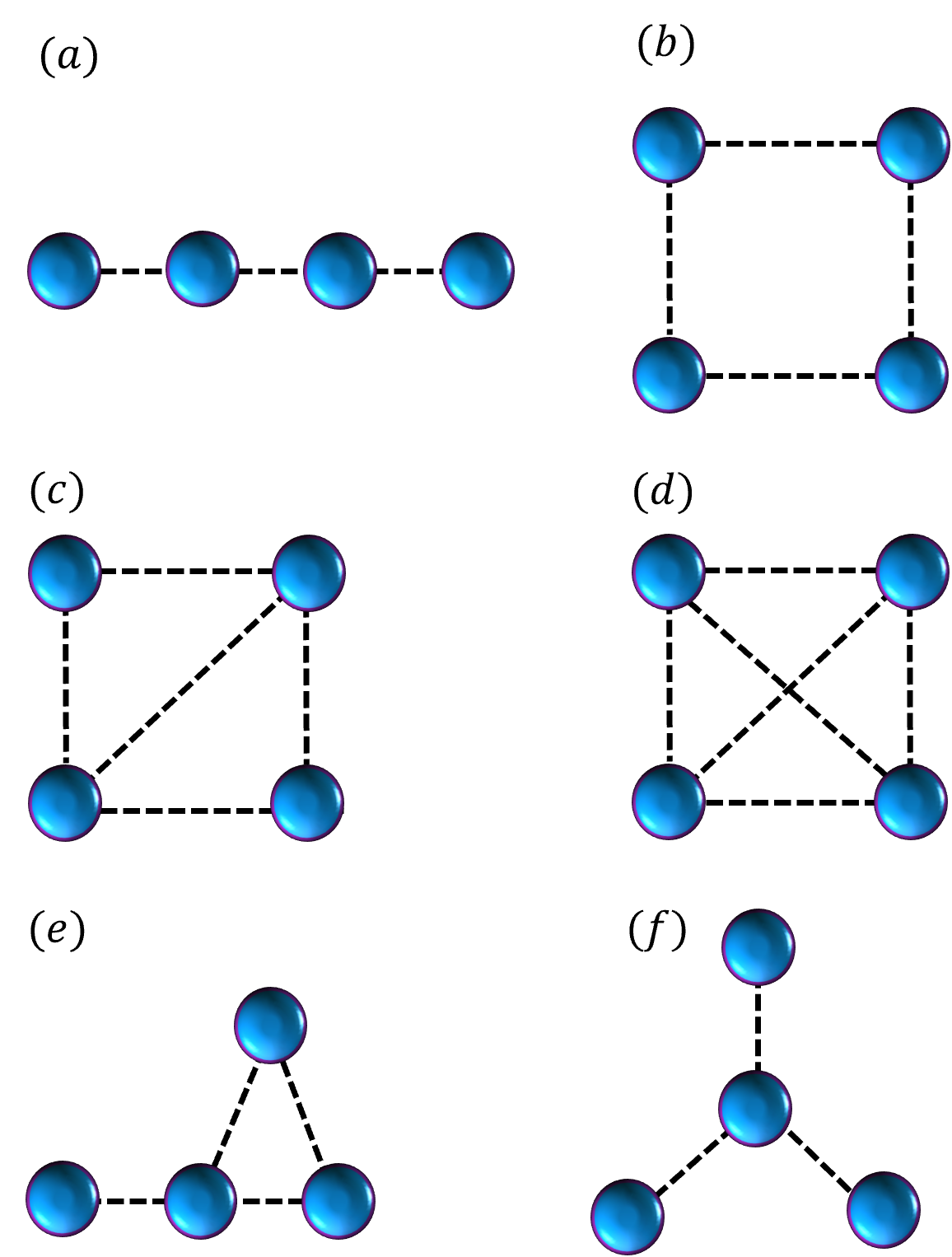
Figure 2: Graphical representation of the structural arrangement of four spins in six different configurations: (a) Chain ($P_{4}$), (b) $4$-cycle square ($C_{4}$), (c) $4$-cycle with a diagonal ($Sd_{4}$), (d) Complete ($K_{4}$), (e) Triangle with a pendant vortex (pan graph), (e) Star-tree graph ($S_{3}$). In each configuration, the spins are coupled to a thermal bath at temperature $T$ and subjected to an external magnetic field of strength $h$. The vertices, represented by solid purple spheres, denote the spin qubits, while the dashed lines indicate the interactions between them.

Index	Graph	No. of Edges	Total degree	Ground state degeneracy
(a)	$P_{4}$	3	6	2
(b)	$C_{4}$	4	8	2
(c)	$Sd_{4}$	5	10	2
(d)	$K_{4}$	6	12	6
(e)	Pan	4	8	6
(f)	$S_{3}$	3	6	2

Table 1: Properties of the six graph configurations. The ”Degree” refers to the sum of the degrees of all nodes, and ”Degeneracy” refers to the number of distinct ground state degeneracies in the absence of an external magnetic field ($h=0$) for the graph.

The Hamiltonian of the quantum sensor composed of $N=4$ qubits governed by the transverse field Ising model is given by (we set $\hbar=k_{B}=1$) Fischer and Hertz (1991); Landau and Lifshitz (2013):

$$\hat{H}_{S}=-\sum_{i>j=1}^{4}J_{ij}\hat{\sigma}_{i}^{z}\hat{\sigma}_{j}^{z}-h_{x}\sum_{i=1}^{4}\hat{\sigma}_{i}^{x},$$ (11)

where $J_{ij}$ represents the coupling strength between qubits, $\hat{\sigma}_{i}^{z}$ and $\hat{\sigma}_{j}^{z}$; $\hat{\sigma}^{\alpha}$ ($\alpha=x,y,z$) are the Pauli operators; and $h_{x}$ denotes the strength of the external magnetic field. For simplicity, we assume homogeneous coupling such that $J_{ij}=J$ and homogeneous magnetic field strength $h_{x}=h$ throughout the paper.

The sign of the coupling constant $J$ determines whether the system exhibits ferromagnetic or antiferromagnetic behavior:

• For ferromagnetic coupling ($J>0$), the qubits tend to align in the same direction, promoting long-range ferromagnetic order.

• For antiferromagnetic coupling ($J<0$), the qubits prefer to align in opposite directions, favoring a more disordered or anti-aligned state.

In this study, we explore both ferromagnetic ($J=1$) and antiferromagnetic ($J=-1$) configurations, considering their effects on quantum sensor performance.

The goal is to use this quantum sensor as a probe to measure the temperature $T$ of the thermal bath and the external magnetic field $h$ (see Fig. 1). Notably, our quantum sensing scheme does not rely on any external drive or strong nonlinear coupling to the environment. Instead, we consider a standard thermodynamic scenario, where a system in contact with a thermal bath at temperature $T$ undergoes thermalization and eventually reaches equilibrium at the same temperature. While many quantum probing schemes focus on extracting parameter information from non-equilibrium dynamics Aiache et al. (2024); Sekatski and Perarnau-Llobet (2022); Cavina et al. (2018); Sekatski and Perarnau-Llobet (2022); Feyles et al. (2019); Albarelli et al. (2023); Mancino et al. (2020); Razavian et al. (2019); Mitchison et al. (2020); Ravell Rodríguez et al. (2024); Paris (2015), our work considers quantum sensors at or near thermal equilibrium—a setting that, although potentially less optimal in speed or coherence usage, aligns more closely with realistic experimental conditions.

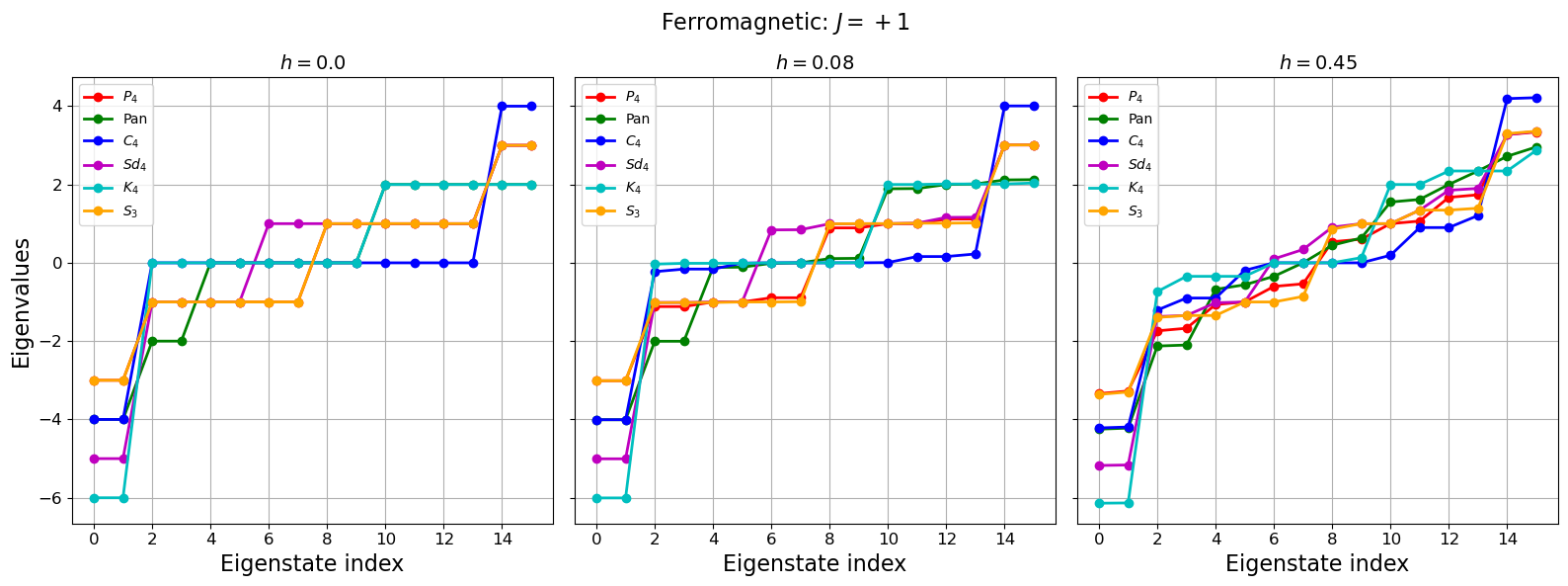
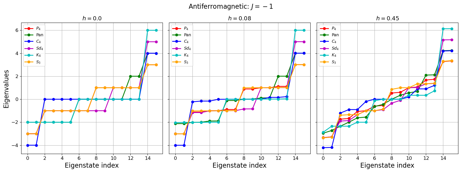
Figure 3: Energy eigenvalue spectra for six different configurations of the quantum sensor in the presence of a weak external magnetic field ($h=0.08$). The top panel corresponds to ferromagnetic coupling ($J=1$) and the bottom panel to antiferromagnetic coupling ($J=-1$). The legends refer to six different configurations of the $4-$qubit quantum sensor, which are given in Fig. 2.

We assume that the system is coupled to a low-temperature bath and subjected to a weak external magnetic field. Under these conditions, the sensor reaches thermal equilibrium with the bath while experiencing the field $h$. Consequently, the system’s state can be well described by the Gibbs thermal state:

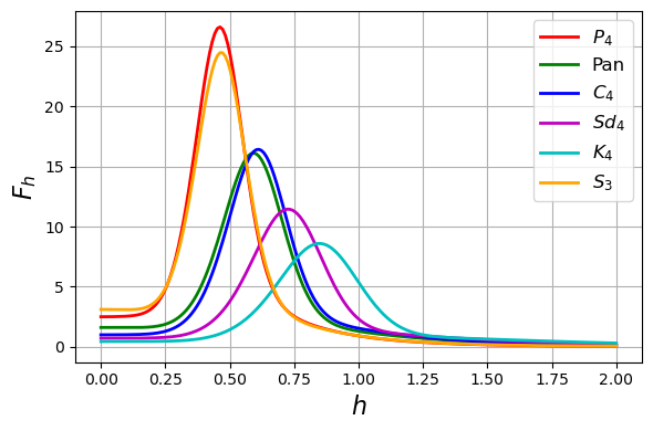
(a)

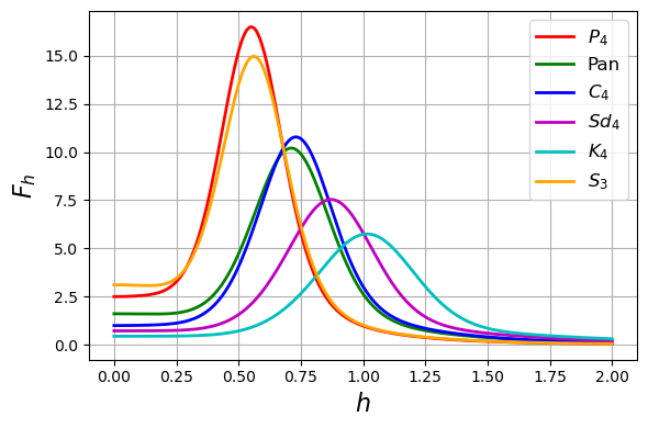
(b)

Figure 4: The QFI ($F_{h}$) for magnetic field ($h$), is plotted as a function of the magnetic field strength $h$ for different quantum sensor configurations at temperatures $T=0.04$ (a) and $T=0.08$ (b). The different colors, such as red, green, blue, magenta, cyan, and orange, represent the configurations $P_{4}$, $C_{4}$, Pan, $Sd_{4}$, $K_{4}$, and $S_{3}$, respectively. All plots correspond to the ferromagnetic coupling ($J=1$).

$$\rho_{G}(T,h)=\frac{\text{exp}{(-\beta\hat{H}_{S})}}{\mathcal{Z}(T,h)},$$ (12)

where $\beta=1/T$ (we set $k_{B}=1$) is the inverse temperature and

$$\mathcal{Z}(T,h)=\text{Tr}\big{[}\text{exp}(-\beta\hat{H}_{S})\big{]}$$ (13)

is the partition.

In the current setting, the QFI is used to analyze the sensor’s ability to individually estimate both the magnetic field $h$ and the temperature $T$. We numerically compute the QFI using the eigenvalues and eigenvectors of $\rho_{G}(T,h)$ to quantify the precision of parameter estimation for both $h$ and $T$ Zhang et al. (2022b).

IV Results

In this section, we present our results of our quantum sensing scheme for the estimation of the magnetic field $h$ and thermal bath temperature $T$. We discuss two cases: ferromagnetic Ising model ($J=1$) and the antiferromagnetic Ising model ($J=-1$). We perform exact diagonalization of the Hamiltonian $\hat{H}(h)$ to obtain its eigenvalues $E_{n}$ and eigenvectors $|\psi_{n}\rangle$ and then construct the thermal state where the populations are given by $p_{n}=e^{-\beta E_{n}/\mathcal{Z}}$. The derivative of the eigenvectors with respect to a parameter $\lambda$ are evaluated by taking the derivative the characteristic equation $\hat{H}|\psi_{n}\rangle=E_{n}|\psi_{n}\rangle$ and rearranging terms, arriving at

$$|\partial_{\lambda}\psi_{n}\rangle=\sum_{m\neq n}\frac{\langle\psi_{m}|\partial_{\lambda}\hat{H}|\psi_{n}\rangle}{E_{n}-E_{m}}|\psi_{m}\rangle,$$ (14)

where $\partial_{\lambda}\hat{H}$ is known from the model (i.e., $-\sum_{i}\hat{\sigma}^{x}$ in the transverse field Ising model).

IV.1 Ferromagnetic sensors of magnetic field

We first assume that the temperature of the thermal bath is known and use Eq. (10) to calculate the QFI for estimation of the magnetic field $h$. We set the interaction between the qubits to $J=1$. Figure 4 presents the QFI as a function of the magnetic field $h$ for the different sensor configurations shown in Fig. 2. Each curve in Fig. 4 corresponds to a specific structural arrangement of the four-qubit sensor, allowing for a comparative analysis of how different configurations influence the estimation precision of $h$.

In the linear-chain configuration ($P_{4}$), the four qubits are arranged in a 1D array with nearest-neighbor interactions. This structure exhibits the largest response to the weak magnetic field, with a gradual increase in QFI as $h$ increases, as shown by the red curve in Fig. 4(a). The QFI of the star graph ($S_{3}$) is slightly lower than that of $P_{4}$ (orange curve) because both graphs have the same energy spectrum, in particular ground states in the weak field regime as shown in Fig. 3 (top panel). In both cases, the QFI rises sharply at a certain value of the magnetic field $h$, reaching the maximum value $F_{\text{max}}$. Both graphs are less symmetric, with only three edges, and possess a simple energy spectrum with 2-fold ground state degeneracy (see Fig. 3 for $h=0$ and Table 1 for graphs properties), making it easier to flip spins at small $h$ because the graphs are more fragile. At small $h$, the system is dominated by the Ising interaction. Due to the minimal connectivity of $P_{4}$ and $S_{3}$, local spin flips cost relatively little energy, resulting in many accessible low-energy states. Even a weak transverse field efficiently mixes these states, creating coherent superpositions (quantum fluctuations) and leading to a large QFI. The magnetic sensitivity is highest at low fields when the temperature is low; however, it decreases, and the maximum slightly shifts toward higher magnetic fields as the temperature increases, as quantum fluctuations become washed out. The increase in temperature helps to melt the fragility of the graphs, making the spin flip easier. This means that higher temperatures degrade the metrological performance in estimation of $h$ (see Fig. 10 in Appendix B for more details).

On the other hand, $C_{4}$ configuration (Fig. 2(b)) where the four qubits form a square lattice with interactions only between nearest-neighbor pairs along the edges, excluding diagonal couplings. While Fig. 2(e) represents the triangle with pendant vertex (pan graph) configuration, where three qubits form a triangular structure with the fourth qubit attached via a single interaction. Interestingly, these two configurations give nearly the same magnetic sensing precision shown by blue and green curves in Fig. 4(b), respectively. This is possible because both graphs are more connected than the chain or star graphs with the same edges, degree, and ground state degeneracy., As a result, the local spin flips become costly in energy. The maximum of QFI also slightly shifts towards the higher magnetic field.

Adding one additional diagonal interaction to the square configuration creates a 4-cycle square with a diagonal ($Sd_{4}$). As shown by the magenta curve in Fig. 4(b), the QFI further decreases due to the extra connection, shifting the maximum towards a higher magnetic field. If the configuration has even more connections, such as the complete graph ($K_{4}$) with all possible diagonal interactions (see Fig. 2(d)), the Ising part couples the spins strongly, even for large $h$. This high connectivity of the graph with the largest degree generates nontrivial correlations that persist against the magnetic field and make the graph stiffer. Therefore, this graph is better for enhancing the magnetic precision at higher values of $h$. Although increasing the temperature reduces the sensitivity in all cases, however, the overall collective behavior remains similar (as shown in Fig. 10 of Appendix B).

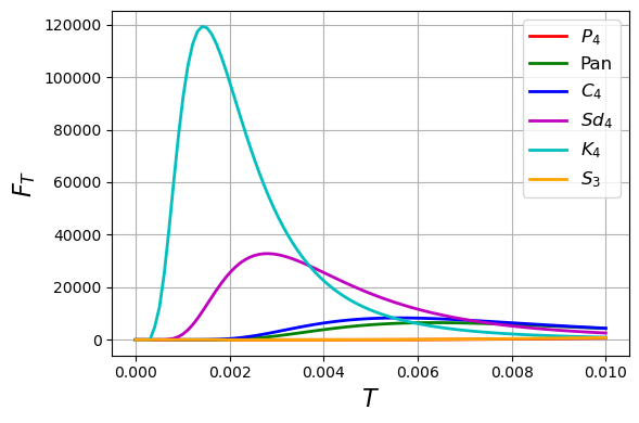
(a)

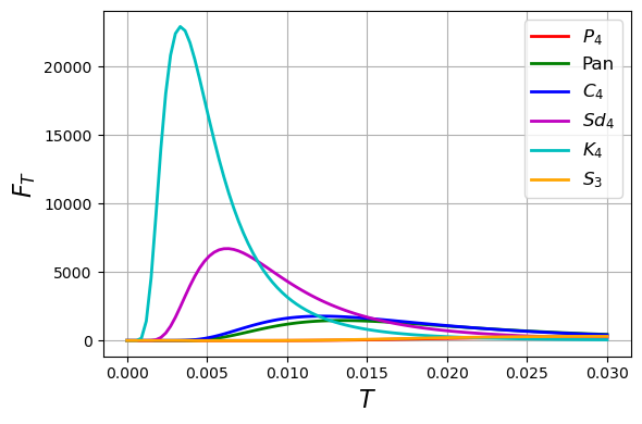
(b)

Figure 5: The QFI ($F_{T}$) temperature estimation is plotted as a function of temperature $T$ for two values of magnetic fields $h=0.45$ (a) and $h=0.55$ (b). The different colors, such as red, green, blue, magenta, cyan, and orange, represent the configurations $P_{4}$, $C_{4}$, Pan, $Sd_{4}$, $K_{4}$, and $S_{3}$, respectively. All plots correspond to the ferromagnetic coupling ($J=1$).

These results show that when the coupling between spins is ferromagnetic ($J=1$), the connectivity and symmetry of the sensor configuration play an important role in determining performance (see Table. 1 for more details). We observe that a sensor with minimal connectivity, such as a chain, is optimal for weak magnetic field estimation (low $h$), whereas a complete graph with more connections is better for high-field sensitivity, although the maximum precision is somewhat reduced. The QFI $F_{h}$ for the estimation of the magnetic field $h$ is linked with the magnetic susceptibility $\chi_{M}$ ($F_{h}\sim\chi_{M}$), which means that the larger the $\chi_{M}$, the greater will be the QFI yielding the maximum precision for magnetic field estimation.

IV.2 Ferromagnetic thermometers

In the previous section, we employed the quantum sensor as a magnetometer and compared the performance of different sensor configurations in estimating the magnetic field with high precision. In this section, we assume that the magnetic field is known and instead, we utilize the sensor as a thermometer to measure the temperature of the thermal bath, and we analyze the effectiveness of various structural configurations in temperature estimation. As we assume that the sensor is at thermal equilibrium with the bath of temperature $T$ in the presence of the external magnetic field $h$, we can also use thermal QFI $F_{th}$ to calculate the QFI for a thermal state $\rho_{th}$ which can be linked to the heat capacity, and hence it turns out to proportional the variance of the sensor Hamiltonian that is given by Mehboudi et al. (2019)

$$F_{th}=\frac{\Delta\hat{H}_{p}^{2}}{T^{4}}=\frac{\langle\hat{H}_{p}^{2}\rangle-\langle\hat{H}_{p}\rangle^{2}}{T^{4}},$$ (15)

where $\langle\hat{H_{p}}\rangle=\text{Tr}[\rho_{th}\hat{H}_{p}]$ represents the expectation of the value of the probe Hamiltonian $\hat{H_{p}}$ for a thermal state $\rho_{th}$. It is important to highlight that the Cramér-Rao bound is saturated at any temperature when the probe is measured in the energy eigenbasis Stace (2010), where the thermal state $\rho_{th}$ remains diagonal. Consequently, in equilibrium thermometry, enhancing precision is only possible by increasing the thermal QFI through careful engineering of the probe.

The QFI as a function of temperature $T$ for various sensor configurations is illustrated in Fig. 5 for two values od temperature. We investigate the influence of the magnetic field $h$ on the precision of temperature estimation by considering two different values of $h$, focusing on the ferromagnetic case where $J=1$. Our analysis indicates that the $K_{4}$ graph exhibits the highest sensitivity for temperature estimation, followed by the $Sd_{4}$ and $C_{4}$ structures. This behavior can be attributed to their respective energy spectra, as illustrated in Fig. 3, where the $K_{4}$ configuration has the lowest ground state energy, followed by $Sd_{4}$ and then $C_{4}$. Notably, their precision in temperature estimation aligns with this ordering, suggesting a correlation between the ground state energy structure and thermometric performance. We note that the temperature precision is maximal at very low temperatures and decreases rapidly as the temperature increases (see Fig. 5(a)).

Furthermore, we find that stronger magnetic fields have a detrimental effect on temperature estimation precision (see Fig. 5(b)). Notably, when $h=0.55$, the highest sensitivity is still exhibited by $K_{4}$. It is interesting to observe that the $K_{4}$ graph, shown in Fig. 2(d), features the maximum number of interactions among the qubits. For instance, the graphs with a greater number of edges and degree are stiffer (see properties of $Sd_{4}$ and $K_{4}$ in Table. 1) and yield greater thermometric precision in the presence of a strong external magnetic field.

IV.3 Antiferromagnetic sensors of magnetic field

We now consider the case of antiferromagnetic couplings such as $J=-1$ and show the results in Fig. 6 for estimation of magnetic field for two values of $T$.

It is immediately evident that the QFI yields entirely different results when the sign of $J$ is reversed. In this case, the pan graph exhibits the highest QFI for magnetic field estimation (green curve in Fig. 6(a)), while the complete graph ($K_{4}$) ranks second (cyan curve in Fig. 6(a)). The high precision achieved by the pan configuration lies in the weak magnetic field regime, whereas $K_{4}$ shows better sensitivity at higher magnetic fields due to its greater connectivity when $T=0.04$ in both cases. However, when the temperature is increased to $T=0.08$, the precision significantly decreases (see Appendix B for the effect of $T$ on the estimation precision of $h$). Of particular importance is the fact that while the other graphs also exhibit nonzero QFI, their values remain much smaller compared to the pan and $K_{4}$ sensors.

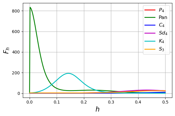
(a)

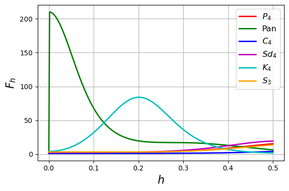
(b)

Figure 6: The QFI ($F_{h}$) for magnetic field estimation is plotted as a function of the magnetic field strength $h$ for different quantum sensor configurations at temperatures $T=0.04$ (a) and $T=0.08$ (b). The different colors, such as red, green, blue, magenta, cyan, and orange, represent the configurations $P_{4}$, $C_{4}$, Pan, $Sd_{4}$, $K_{4}$, and $S_{3}$, respectively. All plots correspond to the antiferromagnetic coupling ($J=-1$)

The variation in magnetic field precision across different structures can be understood by analyzing the eigenvalue spectra of each network. To illustrate this, we compare the spectra of two graphs: the $C_{4}$ structure, which exhibits the lowest QFI, and the pan graph, which achieves the highest QFI for magnetic field sensing. Fig. 3 presents the eigenvalue spectra for these two graphs for different values of $h$ when $J=-1$ (see bottom panel).

In Fig. 3 (bottom panel), we present the eigenvalue spectrum for all six graphs when $h=0,0.08,0.45$ and $J=-1$. For $h=0$, the $C_{4}$ has only the two lowest degenerate energy levels, with most of the zero-energy levels that are also degenerate. Upon applying the external magnetic field (such as $h=0.45$), these energy levels shift, as shown in Fig. 3 (bottom panel). The eigenvalue spectrum of $C_{4}$ reveals four eigenvalues that still remain degenerate at zero energy, which may not have a significant impact at low temperatures. Meanwhile, most of the other eigenvalues form nearly symmetric pairs. We note that it still has a nearly degenerate ground state in the weak field regime (see Appendix A for more details). Therefore, this structure suggests that the energy spectrum is not highly sensitive to small variations in the magnetic field. The magnetic field term, $h\sum_{i}\hat{\sigma}_{i}^{x}$, primarily shifts the energy levels, lifting degeneracies and modifying the spectrum. For instance, in Fig. 3 (bottom panel), the higher degenerate levels that were observed at $h=0$ are slightly split when the field is increased to $h=0.08$ or $h=0.45$, indicating a moderate lifting of degeneracy due to the weak transverse field, and they are still clustered around the zero line. However, due to the pairing symmetry, the energy gaps between levels remain largely unchanged with variations in $h$. Consequently, the high degree of spectral symmetry in the $C_{4}$ energy structure limits its sensitivity to $h$, leading to reduced precision in estimating $h$.

On the other hand, the eigenvalue spectrum of the pan graph and $K_{4}$, shown in Fig. 3(bottom panel), displays six lowest degenerate levels (ground state) at $h=0$. However, when a small transverse field $h=0.45$ is applied, all these six low-energy levels in these two graphs experience noticeable splitting due to degenerate perturbation effects. Unlike the $C_{4}$ configuration, these shifts are more substantial, indicating that the low-energy spectrum of the pan graph is highly sensitive to the magnetic field as compared to the $K_{4}$. Therefore, among the configurations considered, the pan graph exhibits the largest and sharpest spectrum changes with the magnetic field strength (see Fig. 9 for more details), indicating a strong sensitivity to $h$ in the low-energy sector.

Furthermore, the spectrum of the pan graph at $h=0.45$ contains a single zero eigenvalue, indicating a unique high-energy state or a less degenerate excited subspace. The absence of pairing in the low-energy levels or ground state implies that the energy gaps are more susceptible to perturbations from the magnetic field. The increased sensitivity of the energy spectrum to $h$ arises because the energy levels are not constrained by pairing symmetries, allowing for more flexible shifts in response to changes in $h$ (see Fig. 3). As a result, the QFI is higher for the pan graph configuration. Similarly, the energy spectrum of $K_{4}$ graph also does not have degenerate ground states, and it also shows higher QFI (see QFI in Figs. 7(a) and (b)). In summary, the more irregular the spectrum and the absence of nearly ground-state degeneracy in the spectrum, the higher the sensitivity to magnetic field perturbations, highlighting a key design principle for optimizing quantum sensing performance.

IV.4 Antiferromagnetic thermometers

The QFI as a function of temperature T for various structures of the quantum sensor is illustrated in Fig. 7 when antiferromagnetic coupling $J=-1$ is considered between the qubits. Our results reveal that the $C_{4}$ graph exhibits the highest sensitivity for temperature estimation (blue curve in Fig. 7(a)), while the precision achieved by other configurations is small. Furthermore, we observe that stronger magnetic fields have a detrimental effect on the precision of temperature estimation (see Fig. 7(b) where $h=0.55$). It is interesting to note that the maximum interactions between the qubits are present in the $K_{4}$ graph depicted in Fig. 2(d). For this configuration, the temperature precision is the least compared to all other graphs, which shows that maximum connectivity does not help in temperature sensing for $J=-1$.

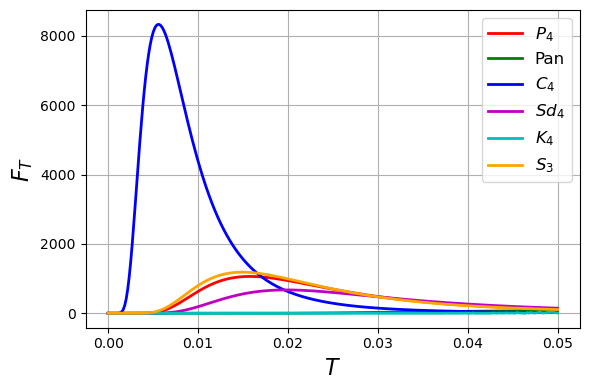
(a)

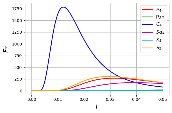
(b)

Figure 7: The QFI ($F_{T}$) for temperature estimation is plotted as a function of temperature $T$ for two values of magnetic fields $h=0.45$ (a) and $h=0.55$ (b). The different colors, such as red, green, blue, magenta, cyan, and orange, represent the configurations $P_{4}$, $C_{4}$, Pan, $Sd_{4}$, $K_{4}$, and $S_{3}$, respectively. All plots correspond to the antiferromagnetic coupling ($J=-1$).

We examine the rate of the Boltzmann factor for each structure to determine why different configurations yield varying temperature precision. The Boltzmann factor governs the probability of a system being in a particular state at temperature $T$, such that $P(\sigma)\propto e^{-\beta\hat{H}(\sigma)}$, where $\hat{H}(\sigma)$ is the energy of a given spin configuration $\sigma$ and $\beta=1/k_{B}T$. To analyze the system’s response to temperature changes, we compute the rate of change of the full Boltzmann distribution with respect to temperature. For each eigenstate with energy $E_{i}$, the Boltzmann weight is given by

$$p_{j}(T)=\frac{e^{-\beta E_{j}}}{\mathcal{Z}(T)},$$ (16)

where $\beta=\frac{1}{k_{B}T}$ and $\mathcal{Z}(T)=\sum_{j}e^{-\beta E_{j}}$ is the partition function. In particular, we focus on the ground state population $p_{0}(T)$, where $E_{0}$ is the lowest energy eigenvalue. Temperature sensitivity may be then assessed by the derivative

$$\frac{d}{dT}p_{0}(T)=\frac{p_{0}(T)}{T^{2}}\left(E_{0}-\bar{E}\right),\qquad\bar{E}=\sum_{j}p_{j}(T)E_{j}.$$ (17)

which characterizes how the thermal population of the ground state changes with temperature. This approach allows us to quantify the sensitivity of the ground state to temperature changes and compare the performance of different configurations in temperature sensing. In Fig. 8, we plot the rate of change of Boltzmann factor $dp_{0}(T)/dT$ as a function of bath temperature $T$ for different configurations. We can see that the configuration with the highest QFI (Fig. 2(b)) corresponds to the one with the sharpest change in $dp_{0}(T)/dT$ values at low temperature, as can be seen by the red dashed curve in Fig. 8, indicating that it is the most sensitive to temperature changes and thus provides the highest precision in temperature estimation. However, when $J=-1$, the sharpest variation in the temperature derivative of the Boltzmann factor is observed for configuration $K_{4}$, in agreement with our earlier predictions shown in Fig. 5. Moreover, the QFI maximum also lies in the same low-temperature regime. In contrast, the other configurations show relatively smooth and less pronounced variations, meaning their temperature sensitivity—and consequently their QFI—remains lower.

Degeneracy plays a crucial role in enhancing precision and expanding the measurable temperature range in quantum thermometry Correa et al. (2015); Campbell et al. (2018). In our setup, this precision improvement arises specifically from the degeneracy of energy levels in the $C_{4}$ configuration, as illustrated in Fig. 3(bottom panel). The pairing of eigenvalues, particularly the presence of nearly degenerate ground states in the $C_{4}$ graph, indicates a high degree of spectrum symmetry and ground state degeneracy. Both the $C_{4}$ and $K_{4}$ graphs feature zero eigenvalues; however, these may not have a significant impact at low temperatures. By contrast, both the pan and $K_{4}$ graphs exhibit a less symmetric spectrum with not much pairing and do not exhibit nearly degenerate ground states. Therefore, this spectrum is advantageous for magnetic sensing but not for temperature. These observations reinforce that the structure of the energy spectrum, particularly its graph and spectral symmetry and degeneracy—plays a critical role in determining the precision of temperature estimation.

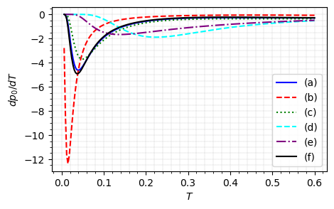
Figure 8: Rate of change of Boltzmann factor $dp_{0}/dT$ for the ground state as a function of temperature $T$. The different curves correspond to the configurations labeled (a), (b), (c), (d), and (e), illustrating their sensitivity to temperature changes. The rest of the parameters are set to $J=-1$ and $h=0.5$.

From these observations, we conclude that compared to the other five structures/configurations investigated in this study, the $C_{4}$ structure demonstrates superior performance in terms of estimation precision of $T$, particularly in the low-temperature regime (when $J=-1$). While the other configurations exhibit varying degrees of sensitivity, none surpass the precision achieved by the $C_{4}$ structure. Note that qubit connectivity plays a crucial role in temperature sensing, where graph symmetry alone does not determine the optimal sensing configuration. While $K_{4}$ is highly symmetric, it is suboptimal for thermometry when $J=-1$. In contrast, $C_{4}$ has lower symmetry but performs optimally for temperature sensing. This highlights the importance of the interplay of the graph topology and spectral structure of the network Hamiltonian in optimizing quantum sensor performance for temperature estimation.

We can further note that the higher temperatures result in lower QFI values across all $h$, highlighting the detrimental impact of thermal fluctuations on parameter estimation. These findings suggest that low-temperature regimes are optimal for magnetic field sensing with enhanced precision, particularly for weak fields. However, as $T$ increases, thermal fluctuations dominate, leading to a loss of estimation precision of $h$. Among all configurations considered, a pan graph and $K_{4}$ graph yield the highest QFI due to the absence of ground state degeneracy, indicating their superior performance for more precise magnetic field estimation, especially in the low-temperature and weak-field regime.

V Role of degeneracy and energy deformation

In this section, we discuss how ground state degeneracy and energy spectrum deformation can also serve as indicators of enhanced quantum sensitivity to magnetic fields. These quantifiers can provide valuable guidelines for identifying the graph structures that are most sensitive to the external magnetic field, especially in scenarios that involve many qubits where direct calculation of the QFI becomes computationally expensive. Thus, analyzing degeneracy and energy deformation offers an efficient alternative to pinpoint configurations with optimal metrological performance without full QFI evaluation.

V.1 Spectral Sensitivity Measure

In quantum sensing applications, one needs to identifying systems with enhanced sensitivity to small external perturbations is essential. One approach is to study the response of the Hamiltonian spectrum under a weak magnetic perturbation parameter, such as the magnetic field $h$. For a system with Hamiltonian

$$\hat{H}(h)=\hat{H}_{0}+h\hat{V},$$ (18)

where $h$ is a small parameter and $\hat{V}$ is a perturbing observable, we find a global spectral deformation measure such as

$$D_{n}(h)=\sqrt{\sum_{i=1}^{n}(E_{i}(h)-E_{i}(0))^{2}},$$ (19)

where $E_{i}(h)$ are the small eigenvalues of $\hat{H}(h)$. This quantity reflects the total deformation of the energy spectrum of the system and is useful in computing the sensitivity of different configurations, such as spin networks defined on different graphs. A large value of $D_{n}(h)$ indicates a strong spectral response to $h$, which suggests higher sensitivity and, in turn, a larger value of the QFI for estimation of $h$.

V.2 Degeneracy and sensitivity

While $D_{n}(h)$ captures the global deformation of the spectrum, it does not fully capture the metrological usefulness of the deformation. In particular, two systems may have the same value of $D_{n}(h)$, yet one may be more useful for parameter estimation if it has a degenerate ground state. Therefore, it is important to mention that degeneracy can significantly enhance the QFI, which bounds the precision of estimating $h$.

To understand this, we perform a perturbative analysis of the QFI in the presence of ground state degeneracy. We consider a $g$-fold degenerate ground state $\{|\psi_{j}^{(0)}\rangle\}_{j=1}^{g}$ of the unperturbed Hamiltonian $\hat{H}_{0}$, all sharing the eigenvalue $E_{0}$. A small perturbation of the form $h\hat{V}$ couples these ground states to the excited states $|\psi_{k}^{(0)}\rangle$ of $\hat{H}_{0}$, potentially lifting the degeneracy.

Let the system be initialized in a uniform superposition over the degenerate ground space

$$|\psi^{(0)}\rangle=\frac{1}{\sqrt{g}}\sum_{j=1}^{g}|\psi^{(0)}_{j}\rangle.$$ (20)

Applying time-independent non-degenerate perturbation theory, the first-order correction to each ground state due to $V$ is

$$|\delta\psi_{j}\rangle=h\sum_{k\notin\text{deg.}}\frac{\langle\psi^{(0)}_{k}|V|\psi^{(0)}_{j}\rangle}{E^{(0)}_{k}-E_{0}}|\psi^{(0)}_{k}\rangle.$$ (21)

The perturbed ground state becomes

$$|\psi_{j}(h)\rangle=|\psi^{(0)}_{j}\rangle+|\delta\psi_{j}\rangle+\mathcal{O}(h^{2}).$$ (22)

The QFI for estimating $h$ in the case of a pure state $|\psi(h)\rangle=\frac{1}{\sqrt{g}}\sum_{j=1}^{g}|\psi_{j}(h)\rangle$ is given by

$$F_{Q}(h)=4\left(\langle\partial_{h}\psi(h)|\partial_{h}\psi(h)\rangle-|\langle\psi(h)|\partial_{h}\psi(h)\rangle|^{2}\right),$$ (23)

where the $\partial_{h}$ denotes the partial derivative with respect to $h$. To leading order in $h$, we can obtain

$$F_{Q}(h)=4h^{2}\left[\frac{1}{g}\sum_{j=1}^{g}\sum_{k\notin\text{deg.}}\left|\frac{\langle\psi^{(0)}_{k}|V|\psi^{(0)}_{j}\rangle}{E^{(0)}_{k}-E_{0}}\right|^{2}\right]+\mathcal{O}(h^{3}).$$ (24)

This shows explicitly that the presence of ground state degeneracy $g$ can enhance the QFI in the small $h$ regime, independent of the total spectral deformation $D_{n}(h)$. Thus, even for fixed $D_{n}$, the graph or system with a higher degeneracy may provide superior metrological precision. In the following, we discuss two examples of graphs composed of 4 spins using the Ising model.

For each graph, we construct the zero transverse field Ising Hamiltonian and analyze its ground state structure. After that, we compute the spectral sensitivity measure $D_{n}(h)$, which quantifies the trace distance between the unperturbed and perturbed spectra under small field perturbations. Finally, we calculate the ground state degeneracy to explore its connection to the QFI.

In particular, we evaluate $D_{n}(h)$ by calculating the unperturbed ground state energy $E_{0}$ when $h=0$, its degeneracy $g$, and the spectral deviation $D_{n}(h)$ under a small transverse field perturbation of the form $\sum_{i}\hat{\sigma}_{i}^{x}$. It is important to note that some graphs can still exhibit similar values of $D_{n}(h)$; however, due to their different ground state degeneracies, their sensitivity to $h$ can be different. Notably, the pan graph shows both a large$D_{n}(h)$ value and also a higher degeneracy, suggesting that it may yield a higher QFI, as we have indeed seen in the previous Sections. To understand this behavior, we refer to the perturbative expansion of the QFI in the presence of ground state degeneracy. For a maximally mixed initial state within the degenerate ground state subspace, the QFI is approximately given by

$$F_{Q}(h)\approx\frac{4h^{2}}{g}\sum_{i<j}\frac{|\langle\psi_{i}^{(0)}|\hat{V}|\psi_{j}^{(0)}\rangle|^{2}}{(E_{i}-E_{j})^{2}},$$ (25)

where $g$ is the ground state degeneracy and $\hat{V}=\sum_{i}\hat{\sigma}_{i}^{x}$ is the perturbation operator. Although the prefactor $1/g$ appears due to the mixed-state assumption, the number of contributing off-diagonal terms grows as $g(g-1)/2$. This can result in an overall enhancement of the QFI with increasing degeneracy, provided the energy differences $E_{i}-E_{j}$ are not too large. Consequently, if two graphs have the same spectral deviation $D_{n}$, the one with higher ground state degeneracy will generally yield a higher QFI. This highlights the complementary roles of spectral deviation and degeneracy in determining quantum sensitivity to perturbations.

In the case of ferromagnetic coupling ($J=1$), all six graphs exhibit 2-fold ground state degeneracy for weak magnetic fields (see top panel of Fig. 3). Therefore, we cannot use the $D_{n}(h)$ measure using the unperturbed and perturbed ground states ($E_{0}(h)-E_{0}(0)$) because we can get the same values of quantity $D_{n}(h)$ due to ground state degeneracy in the weak magnetic field regime. To counter this issue, one may consider a perturbed first excited state and calculate $E_{1}(h)-E_{0}(0)$ to see the deformation measure $D_{n}(h)$. This may provide insight into identifying graph structures that offer the highest precision in field estimation.

VI Conclusion

In this work, we have studied the performance of a four-qubit quantum sensor governed by the transverse Ising model, considering all connected graph configurations for applications in magnetometry and thermometry. Our analysis includes both ferromagnetic and antiferromagnetic couplings, assessing their impact on the sensor’s behavior across different geometries. Using the quantum Fisher information (QFI) to quantify precision limits, we have analyzed in detail how the qubit arrangement and the spectral structure of the Hamiltonian determine the sensor’s metrological capabilities.

In the ferromagnetic regime and weak magnetic field, graphs with minimal connectivity, like the linear-chain ($P_{4}$), provide optimal performance due to degenerate ground states and efficient spin flips. The star graph ($S_{3}$) exhibits similar behavior. Conversely, highly connected graphs, such as the complete graph ($K_{4}$), require stronger fields to show significant sensitivity. For estimation of temperature, more connected graphs like $K_{4}$ and $Sd_{4}$ perform better at weaker fields due to their stiffer structure and larger energy gaps. This indicates that low-energy-excitation favoring structures perform well at low temperatures, while stiffer graphs maintain sensitivity in strong fields.

In the antiferromagnetic case, we have identified the triangular configuration with a pendant vortex (termed pan graph) as the most effective for magnetic field estimation, while the $C_{4}$ configuration is better for temperature sensing. We have discussed the differences in magnetic sensing precision across various configurations by analyzing the spectra of their eigenvalues. The $C_{4}$ graph configuration, which exhibits lower sensitivity to magnetic fields, has four exactly zero eigenvalues, with two additional eigenvalues lying very close to zero. This leads to a high degree of degeneracy, including nearly degenerate ground states. Such a spectrum limits the system’s responsiveness to magnetic field perturbations due to degenerate values, thereby lowering the QFI for magnetic field estimation. In contrast, the pan graph configuration, identified as optimal for magnetometry, exhibits a non-degenerate spectrum with only one zero eigenvalue and no pairing symmetries. The absence of nearly degenerate ground states and low symmetry in the spectrum or pairing allows the energy levels to shift more distinctly under external field perturbations, enhancing the system’s sensitivity to the external field $h$. These energy spectrum features of the pan and $K_{4}$ graph configurations make them well-suited for the enhanced precision of magnetic field sensing, while graphs with degenerate energy levels yield the highest QFI for temperature estimation.

Furthermore, the configuration with the highest QFI for temperature estimation exhibits the sharpest variation in the rate of change of the Boltzmann factor as a function of temperature, which further confirms its superior sensitivity to temperature changes. The rapid change in occupation probabilities of energy states in this configuration enhances its response to temperature variations, making it optimal for quantum thermometry. In contrast, other configurations display more gradual variations, leading to lower temperature sensitivity and, hence, a lower QFI. This enhanced temperature sensitivity of the $C_{4}$ graph configuration is due to the degenerate ground states. Our results indicate that low temperatures enhance magnetic field sensing, whereas weak magnetic fields improve temperature estimation. Conversely, strong magnetic fields degrade QFI as a function of temperature.

Our analysis highlights that both the spectral deformation measure $D_{n}(h)$ and the presence of ground state degeneracy crucially influence the sensitivity of parameter estimation. While $D_{n}(h)$ captures global spectral changes, degeneracy can substantially enhance the QFI even when $D_{n}(h)$ is similar across systems. This complementary understanding can be useful for designing graph-based quantum sensors with optimal precision. Our results provide insights into the role of graph connectivity in quantum sensing and highlight how configurational optimization can enhance measurement precision in a multi-qubit sensor. A systematic approach to generalizing our case study to a larger number of qubits or quantum sensor networks may be possible using graph theory. The symmetry of graphs can be analyzed in terms of their automorphism group size, which quantifies the number of ways to relabel the vertices while preserving the adjacency matrix. However, graph symmetry alone does not determine the optimal configuration for sensing. For example, the complete graph $K_{4}$ is not optimal for thermometry despite its high symmetry, as indicated by its large automorphism group of size $24$. This suggests that higher symmetry does not necessarily imply better sensitivity for parameter estimation tasks like temperature sensing.

Appendix A Effect of external magnetic field on energy spectrum

In this Appendix, we examine the eigenvalue spectra for six distinct configurations of the quantum sensor as a function of magnetic field $h$, for an antiferromagnetic coupling ($J=-1$). In Fig. 3 (bottom panel for $J=-1$), we first investigate the case when no external magnetic field is applied ($h=0$). It is immediately apparent that, except for the $K_{4}$ and pan graphs, all other configurations exhibit $2$-fold degenerate ground states. Similarly, the square configuration shows the highest degeneracy in the first excited state. When an external magnetic field is applied, it acts as a perturbation that does not completely lift the degeneracy of $C_{4}$ structure, only slightly shifting the energy levels. However, for a strong magnetic field of $h=0.45$, the ground state degeneracy is lifted, and also the low energy states do not remain degenerate, but this does not benefit the estimation of $h$ . The $C_{4}$ configuration, in particular, tries to maintain symmetry in its energy spectrum, resulting in minimal response to magnetic perturbations, making it a poor candidate for magnetic field sensing. However, it proves to be an excellent probe for temperature sensing, where degeneracy typically enhances measurement precision.

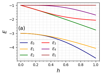
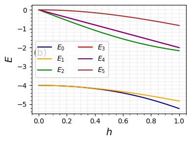
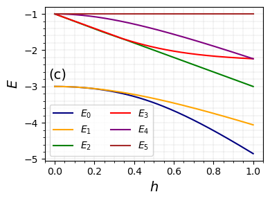
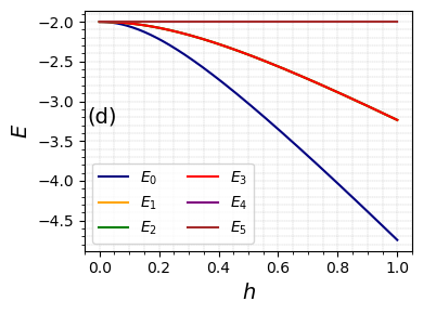
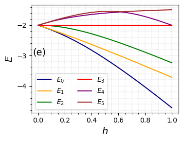
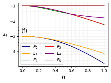
Figure 9: The first six eigenvalues plotted as a function of external magnetic field $h$ for all six different graphs ($N=4$). The coupling strength is fixed at $J=1$. The panel labels (a) to (f) in these plots correspond to six different configurations of the $4$-qubit quantum sensor as shown in Fig. 2.

On the other hand, the $K_{4}$ graph and pan graph both exhibit six degenerate ground states when $h=0$ (see Fig. 3 of the main text). Upon applying an external magnetic field, it acts as a perturbation and lifts the degeneracy. At $h=0.45$, all six energy levels are shifted due to degenerate perturbations. Specifically, for the $K_{4}$ graph, the six degenerate states shift slightly under $h=0.45$, while for the pan graph, all six low-energy levels remain relevant due to greater shift in energy levels, and it shows the most significant change among the configurations under the same external field.

Fig. 9 shows the behavior of the first six eigenvalues as a function of the external magnetic field $h$ for $J=-1$. From these plots, it is evident that all graphs, except for the $K_{4}$ and pan graphs, exhibit nearly degenerate ground states in the weak field regime. This degeneracy is progressively lifted as the magnetic field strength increases, which explains the decrease in temperature precision in the strong magnetic field regime. In contrast, both the $K_{4}$ and pan graphs show a more pronounced shift in the energy levels with no signs of degeneracy. As a result, these two graphs are most responsive to the external magnetic field, making them optimal configurations for magnetic field sensing.

Appendix B Effect of temperature on the estimation of the field

In this section, we present our results on the effect of temperature on the estimation of the parameter $h$ in Fig. 10. We analyze the QFI for different temperature values for ferromagnetic ( $J=1$) and antiferromagnetic ( $J=-1$ ) sensors of magnetic field. Our findings show that increasing temperature drastically reduces the QFI, indicating a significant decline in estimation precision at higher temperatures for both magnetic interaction regimes. Notably, antiferromagnetic sensors still maintain better sensitivity compared to ferromagnetic sensors even at higher temperatures.

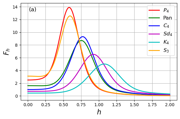
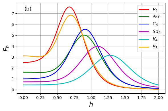
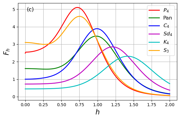
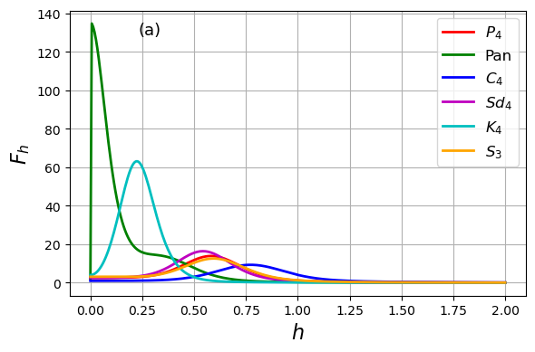
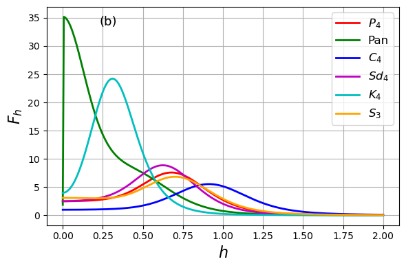
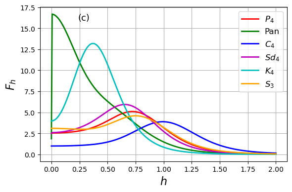
Figure 10: Top panel: QFI $F_{h}$ as a function of magnetic field $h$ for different values of temperature $T$ when $J=1$. Bottom panel: QFI $F_{h}$ as a function of magnetic field $h$ for different values of temperature $T$ when $J=-1$. Here, the legends in each plot correspond to (a) $T=0.1$, (b) $T=0.2$, and (c) $T=0.3$, respectively.

References

- Wang et al. (2018) Zhihai Wang, Wei Wu, Guodong Cui, and Jin Wang, “Coherence enhanced quantum metrology in a nonequilibrium optical molecule,” New J. Phys. 20, 033034 (2018).
- Cheng et al. (2019) Weijun Cheng, S. C. Hou, Zhihai Wang, and X. X. Yi, “Quantum metrology enhanced by coherence-induced driving in a cavity-qed setup,” Phys. Rev. A 100, 053825 (2019).
- Joo et al. (2011) Jaewoo Joo, William J. Munro, and Timothy P. Spiller, “Quantum metrology with entangled coherent states,” Phys. Rev. Lett. 107, 083601 (2011).
- Huang et al. (2016) Zixin Huang, Chiara Macchiavello, and Lorenzo Maccone, “Usefulness of entanglement-assisted quantum metrology,” Phys. Rev. A 94, 012101 (2016).
- Giovannetti et al. (2006) Vittorio Giovannetti, Seth Lloyd, and Lorenzo Maccone, “Quantum metrology,” Phys. Rev. Lett. 96, 010401 (2006).
- Degen et al. (2017) C. L. Degen, F. Reinhard, and P. Cappellaro, “Quantum sensing,” Rev. Mod. Phys. 89, 035002 (2017).
- Tóth and Apellaniz (2014) Géza Tóth and Iagoba Apellaniz, “Quantum metrology from a quantum information science perspective,” J. Phys. A: Math. Theor. 47, 424006 (2014).
- Giovannetti et al. (2011) Vittorio Giovannetti, Seth Lloyd, and Lorenzo Maccone, “Advances in quantum metrology,” Nat. Photonics 5, 222–229 (2011).
- Aslam et al. (2023) Nabeel Aslam, Hengyun Zhou, Elana K. Urbach, Matthew J. Turner, Ronald L. Walsworth, Mikhail D. Lukin, and Hongkun Park, “Quantum sensors for biomedical applications,” Nat Rev. Phys. 5, 157–169 (2023).
- Taylor and Bowen (2016) Michael A. Taylor and Warwick P. Bowen, “Quantum metrology and its application in biology,” Phys. Rep. 615, 1–59 (2016), quantum metrology and its application in biology.
- DeMille et al. (2024) David DeMille, Nicholas R. Hutzler, Ana Maria Rey, and Tanya Zelevinsky, “Quantum sensing and metrology for fundamental physics with molecules,” Nat. Phys. 20, 741–749 (2024).
- Mehboudi et al. (2019) Mohammad Mehboudi, Anna Sanpera, and Luis A Correa, “Thermometry in the quantum regime: Recent theoretical progress,” J. Phys. A: Math. Theor. 52, 303001 (2019).
- Dedyulin et al. (2022) S Dedyulin, Z Ahmed, and G Machin, “Emerging technologies in the field of thermometry,” Meas, Sci. Technol. 33, 092001 (2022).
- Moreva et al. (2020) E. Moreva, E. Bernardi, P. Traina, A. Sosso, S. Ditalia Tchernij, J. Forneris, F. Picollo, G. Brida, Ž. Pastuović, I. P. Degiovanni, P. Olivero, and M. Genovese, “Practical applications of quantum sensing: A simple method to enhance the sensitivity of nitrogen-vacancy-based temperature sensors,” Phys. Rev. Appl. 13, 054057 (2020).
- Wang et al. (2020) J. Wang, L. Davidovich, and G. S. Agarwal, “Quantum sensing of open systems: Estimation of damping constants and temperature,” Phys. Rev. Res. 2, 033389 (2020).
- Brenes and Segal (2023) Marlon Brenes and Dvira Segal, “Multispin probes for thermometry in the strong-coupling regime,” Phys. Rev. A 108, 032220 (2023).
- Gottscholl et al. (2021) Andreas Gottscholl, Matthias Diez, Victor Soltamov, Christian Kasper, Dominik Krauße, Andreas Sperlich, Mehran Kianinia, Carlo Bradac, Igor Aharonovich, and Vladimir Dyakonov, “Spin defects in hbn as promising temperature, pressure and magnetic field quantum sensors,” Nat. Commun. 12, 4480 (2021).
- Klimov et al. (2018) Nikolai Klimov, Thomas Purdy, and Zeeshan Ahmed, “Towards replacing resistance thermometry with photonic thermometry,” Sensors Actuat. A: Phys. 269, 308–312 (2018).
- Li et al. (2010) Bei-Bei Li, Qing-Yan Wang, Yun-Feng Xiao, Xue-Feng Jiang, Yan Li, Lixin Xiao, and Qihuang Gong, “On chip, high-sensitivity thermal sensor based on high-q polydimethylsiloxane-coated microresonator,” Appl. Phys. Lett. 96, 251109 (2010).
- Dong et al. (2009) C.-H. Dong, L. He, Y.-F. Xiao, V. R. Gaddam, S. K. Ozdemir, Z.-F. Han, G.-C. Guo, and L. Yang, “Fabrication of high-q polydimethylsiloxane optical microspheres for thermal sensing,” Appl. Phys. Lett. 94, 231119 (2009).
- Purdy et al. (2017) T. P. Purdy, K. E. Grutter, K. Srinivasan, and J. M. Taylor, “Quantum correlations from a room-temperature optomechanical cavity,” Science 356, 1265–1268 (2017).
- Chowdhury et al. (2019) A Chowdhury, P Vezio, M Bonaldi, A Borrielli, F Marino, B Morana, G Pandraud, A Pontin, G A Prodi, P M Sarro, E Serra, and F Marin, “Calibrated quantum thermometry in cavity optomechanics,” Quantum Sci. Technol. 4, 024007 (2019).
- Singh and Purdy (2020) Robinjeet Singh and Thomas P. Purdy, “Detecting acoustic blackbody radiation with an optomechanical antenna,” Phys. Rev. Lett. 125, 120603 (2020).
- Galinskiy et al. (2020) I. Galinskiy, Y. Tsaturyan, M. Parniak, and E. S. Polzik, “Phonon counting thermometry of an ultracoherent membrane resonator near its motional ground state,” Optica 7, 718–725 (2020).
- Aybar et al. (2022) Enes Aybar, Artur Niezgoda, Safoura S. Mirkhalaf, Morgan W. Mitchell, Daniel Benedicto Orenes, and Emilia Witkowska, “Critical quantum thermometry and its feasibility in spin systems,” Quantum 6, 808 (2022).
- Yu et al. (2024) Mei Yu, H. Chau Nguyen, and Stefan Nimmrichter, “Criticality-enhanced precision in phase thermometry,” Phys. Rev. Res. 6, 043094 (2024).
- Salvatori et al. (2014) Giulio Salvatori, Antonio Mandarino, and Matteo G. A. Paris, “Quantum metrology in lipkin-meshkov-glick critical systems,” Phys. Rev. A 90, 022111 (2014).
- Zhang et al. (2022a) Ning Zhang, Chong Chen, Si-Yuan Bai, Wei Wu, and Jun-Hong An, “Non-markovian quantum thermometry,” Phys. Rev. Appl. 17, 034073 (2022a).
- Mok et al. (2021) Wai-Keong Mok, Kishor Bharti, Leong-Chuan Kwek, and Abolfazl Bayat, “Optimal probes for global quantum thermometry,” Commun. Phys. 4, 62 (2021).
- Zanardi et al. (2008) Paolo Zanardi, Matteo G. A. Paris, and Lorenzo Campos Venuti, “Quantum criticality as a resource for quantum estimation,” Phys. Rev. A 78, 042105 (2008).
- Seah et al. (2019) Stella Seah, Stefan Nimmrichter, Daniel Grimmer, Jader P. Santos, Valerio Scarani, and Gabriel T. Landi, “Collisional quantum thermometry,” Phys. Rev. Lett. 123, 180602 (2019).
- De Daniloff et al. (2021) Clément De Daniloff, Marin Tharrault, Cédric Enesa, Christophe Salomon, Frédéric Chevy, Thomas Reimann, and Julian Struck, “In situ thermometry of fermionic cold-atom quantum wires,” Phys. Rev. Lett. 127, 113602 (2021).
- Glatthard et al. (2022) Jonas Glatthard, Jesús Rubio, Rahul Sawant, Thomas Hewitt, Giovanni Barontini, and Luis A. Correa, “Optimal cold atom thermometry using adaptive Bayesian strategies,” PRX Quantum 3, 040330 (2022).
- Roscilde (2014) Tommaso Roscilde, “Thermometry of cold atoms in optical lattices via artificial gauge fields,” Phys. Rev. Lett. 112, 110403 (2014).
- Brask et al. (2015) J. B. Brask, R. Chaves, and J. Kołodyński, “Improved quantum magnetometry beyond the standard quantum limit,” Phys. Rev. X 5, 031010 (2015).
- Razzoli et al. (2019) Luca Razzoli, Luca Ghirardi, Ilaria Siloi, Paolo Bordone, and Matteo G. A. Paris, “Lattice quantum magnetometry,” Phys. Rev. A 99, 062330 (2019).
- Wasilewski et al. (2010) W. Wasilewski, K. Jensen, H. Krauter, J. J. Renema, M. V. Balabas, and E. S. Polzik, “Quantum noise limited and entanglement-assisted magnetometry,” Phys. Rev. Lett. 104, 133601 (2010).
- Troiani and Paris (2018) Filippo Troiani and Matteo G. A. Paris, “Universal quantum magnetometry with spin states at equilibrium,” Phys. Rev. Lett. 120, 260503 (2018).
- Troullinou et al. (2023) Charikleia Troullinou, Vito Giovanni Lucivero, and Morgan W. Mitchell, “Quantum-enhanced magnetometry at optimal number density,” Phys. Rev. Lett. 131, 133602 (2023).
- Montenegro et al. (2022) Victor Montenegro, Gareth Siôn Jones, Sougato Bose, and Abolfazl Bayat, “Sequential measurements for quantum-enhanced magnetometry in spin chain probes,” Phys. Rev. Lett. 129, 120503 (2022).
- Shukla and Chandrashekar (2024) Kunal Shukla and C. M. Chandrashekar, “Quantum magnetometry using discrete-time quantum walk,” Phys. Rev. A 109, 032608 (2024).
- Li et al. (2018) Bei-Bei Li, Jan Bílek, Ulrich B. Hoff, Lars S. Madsen, Stefan Forstner, Varun Prakash, Clemens Schäfermeier, Tobias Gehring, Warwick P. Bowen, and Ulrik L. Andersen, “Quantum enhanced optomechanical magnetometry,” Optica 5, 850–856 (2018).
- Albarelli et al. (2017) Francesco Albarelli, Matteo A C Rossi, Matteo G A Paris, and Marco G Genoni, “Ultimate limits for quantum magnetometry via time-continuous measurements,” New J. Phys. 19, 123011 (2017).
- Ishizaki and Fleming (2012) Akihito Ishizaki and Graham R. Fleming, “Quantum coherence in photosynthetic light harvesting,” Ann. Rev. Condens. Matter Phys. 3, 333–361 (2012).
- Proctor et al. (2018) Timothy J. Proctor, Paul A. Knott, and Jacob A. Dunningham, “Multiparameter estimation in networked quantum sensors,” Phys. Rev. Lett. 120, 080501 (2018).
- Bringewatt et al. (2021) Jacob Bringewatt, Igor Boettcher, Pradeep Niroula, Przemyslaw Bienias, and Alexey V. Gorshkov, “Protocols for estimating multiple functions with quantum sensor networks: Geometry and performance,” Phys. Rev. Res. 3, 033011 (2021).
- Gassab et al. (2024) Lea Gassab, Onur Pusuluk, and Özgür E. Müstecaplıoğlu, “Geometrical optimization of spin clusters for the preservation of quantum coherence,” Phys. Rev. A 109, 012424 (2024).
- Upadhyay and Marathe (2024) Vipul Upadhyay and Rahul Marathe, “Current circulation near additional energy degeneracy points in quadratic fermionic networks,” J. Stat. Mech. 2024, 113104 (2024).
- Candeloro et al. (2021) Alessandro Candeloro, Luca Razzoli, Paolo Bordone, and Matteo G. A. Paris, “Role of topology in determining the precision of a finite thermometer,” Phys. Rev. E 104, 014136 (2021).
- Lechner et al. (2015) Wolfgang Lechner, Philipp Hauke, and Peter Zoller, “A quantum annealing architecture with all-to-all connectivity from local interactions,” Science Advances 1, e1500838 (2015).
- Nigg et al. (2017) Simon E. Nigg, Niels Lörch, and Rakesh P. Tiwari, “Robust quantum optimizer with full connectivity,” Science Advances 3, e1602273 (2017).
- Campbell et al. (2018) Steve Campbell, Marco G Genoni, and Sebastian Deffner, “Precision thermometry and the quantum speed limit,” Quantum Sci. Technol. 3, 025002 (2018).
- Correa et al. (2015) Luis A. Correa, Mohammad Mehboudi, Gerardo Adesso, and Anna Sanpera, “Individual quantum probes for optimal thermometry,” Phys. Rev. Lett. 114, 220405 (2015).
- Płodzień et al. (2018) Marcin Płodzień, Rafał Demkowicz-Dobrzański, and Tomasz Sowiński, “Few-fermion thermometry,” Phys. Rev. A 97, 063619 (2018).
- Srivastava et al. (2023) Anubhav Kumar Srivastava, Utso Bhattacharya, Maciej Lewenstein, and Marcin Płodzień, “Topological quantum thermometry,” (2023), arXiv:2311.14524 .
- Srivastava et al. (2025) Anubhav Kumar Srivastava, Utso Bhattacharya, Maciej Lewenstein, and Marcin Płodzień, “Topological quantum thermometry,” Phys. Rev. A 111, 052216 (2025).
- Paris (2009) Matteo G. A. Paris, “Quantum estimation for quantum technology,” Intl. J. Quant. Inf. 07, 125–137 (2009).
- Helstrom (1969a) Carl W. Helstrom, “Quantum detection and estimation theory,” J. Stat. Phys. 1, 231–252 (1969a).
- Sidhu and Kok (2020) Jasminder S. Sidhu and Pieter Kok, “Geometric perspective on quantum parameter estimation,” AVS Quantum Sci. 2, 014701 (2020).
- Braunstein and Caves (1994) Samuel L. Braunstein and Carlton M. Caves, “Statistical distance and the geometry of quantum states,” Phys. Rev. Lett. 72, 3439–3443 (1994).
- Helstrom (1969b) Carl W. Helstrom, “Quantum detection and estimation theory,” J. Stat. Phys¿ 1, 231–252 (1969b).
- Fischer and Hertz (1991) K. H. Fischer and J. A. Hertz, Spin Glasses, Cambridge Studies in Magnetism (Cambridge University Press, 1991).
- Landau and Lifshitz (2013) Lev Davidovich Landau and Evgenii Mikhailovich Lifshitz, Statistical Physics: Volume 5, Vol. 5 (Elsevier, 2013).
- Aiache et al. (2024) Y. Aiache, C. Seida, K. El Anouz, and A. El Allati, “Non-markovian enhancement of nonequilibrium quantum thermometry,” Phys. Rev. E 110, 024132 (2024).
- Sekatski and Perarnau-Llobet (2022) Pavel Sekatski and Martí Perarnau-Llobet, “Optimal nonequilibrium thermometry in Markovian environments,” Quantum 6, 869 (2022).
- Cavina et al. (2018) Vasco Cavina, Luca Mancino, Antonella De Pasquale, Ilaria Gianani, Marco Sbroscia, Robert I. Booth, Emanuele Roccia, Roberto Raimondi, Vittorio Giovannetti, and Marco Barbieri, “Bridging thermodynamics and metrology in nonequilibrium quantum thermometry,” Phys. Rev. A 98, 050101 (2018).
- Feyles et al. (2019) Michele M. Feyles, Luca Mancino, Marco Sbroscia, Ilaria Gianani, and Marco Barbieri, “Dynamical role of quantum signatures in quantum thermometry,” Phys. Rev. A 99, 062114 (2019).
- Albarelli et al. (2023) Francesco Albarelli, Matteo G. A. Paris, Bassano Vacchini, and Andrea Smirne, “Invasiveness of nonequilibrium pure-dephasing quantum thermometry,” Phys. Rev. A 108, 062421 (2023).
- Mancino et al. (2020) Luca Mancino, Marco G. Genoni, Marco Barbieri, and Mauro Paternostro, “Nonequilibrium readiness and precision of gaussian quantum thermometers,” Phys. Rev. Res. 2, 033498 (2020).
- Razavian et al. (2019) Sholeh Razavian, Claudia Benedetti, Matteo Bina, Yahya Akbari-Kourbolagh, and Matteo G. A. Paris, “Quantum thermometry by single-qubit dephasing,” The European Physical Journal Plus 134, 284 (2019).
- Mitchison et al. (2020) Mark T. Mitchison, Thomás Fogarty, Giacomo Guarnieri, Steve Campbell, Thomas Busch, and John Goold, “In situ thermometry of a cold Fermi gas via dephasing impurities,” Phys. Rev. Lett. 125, 080402 (2020).
- Ravell Rodríguez et al. (2024) Ricard Ravell Rodríguez, Mohammad Mehboudi, Michał Horodecki, and Martí Perarnau-Llobet, “Strongly coupled fermionic probe for nonequilibrium thermometry,” New J. Phys. 26, 013046 (2024).
- Paris (2015) Matteo G A Paris, “Achieving the landau bound to precision of quantum thermometry in systems with vanishing gap,” J. Phys. A: Math. Theor. 49, 03LT02 (2015).
- Zhang et al. (2022b) Mao Zhang, Huai-Ming Yu, Haidong Yuan, Xiaoguang Wang, Rafał Demkowicz-Dobrzański, and Jing Liu, “Quanestimation: An open-source toolkit for quantum parameter estimation,” Phys. Rev. Res. 4, 043057 (2022b).
- Stace (2010) Thomas M. Stace, “Quantum limits of thermometry,” Phys. Rev. A 82, 011611 (2010).