Intrinsic enumerative mirror symmetry: Takahashi’s log mirror symmetry for $(\mathbb{P}^{2},E)$ revisited

Abstract.

Let $E$ be a smooth cubic in the projective plane $\mathbb{P}^{2}$. Nobuyoshi Takahashi formulated a conjecture that expresses counts of rational curves of varying degree in $\mathbb{P}^{2}\setminus E$ as the Taylor coefficients of a particular period integral of a pencil of affine plane cubics after reparametrizing the pencil using the exponential of a second period integral.

The intrinsic mirror construction introduced by Mark Gross and the third author associates to a degeneration of $(\mathbb{P}^{2},E)$ a canonical wall structure from which one constructs a family of projective plane cubics that is birational to Takahashi’s pencil in its reparametrized form. By computing the period integral of the positive real locus explicitly, we find that it equals the logarithm of the product of all asymptotic wall functions. The coefficients of these asymptotic wall functions are logarithmic Gromov-Witten counts of the central fiber of the degeneration that agree with the algebraic curve counts in $(\mathbb{P}^{2},E)$ in question. We conclude that Takahashi’s conjecture is a natural consequence of intrinsic mirror symmetry. Our method generalizes to give similar results for log Calabi-Yau varieties of arbitrary dimension.

1. Enumerative mirror symmetry is manifest in intrinsic mirror symmetry

1.1. Intrinsic enumerative mirror symmetry

Mirror symmetry is a prediction originating in string theory [CLS, GrPl, CdOGP]. It states that Calabi–Yau manifolds come in mirror families

$$\mathcal{X}_{\tau,s}\longleftrightarrow\widecheck{\mathcal{X}}_{\sigma,t}$$

with $\tau,\sigma$ $A$-model symplectic structure parameters and $s,t$ $B$-model complex structure parameters.

The construction of pairs of mirror families traditionally mostly relied on toric ad hoc constructions [B, BB, BH], but can now be done in great generality in a completely natural fashion via the intrinsic mirror symmetry construction [GHK, GS18, KY23, GS19, GS22, KY24].

Enumerative mirror symmetry, pioneered in [CdOGP], is the conjecture that the $A$-model variation of symplectic structure of $\mathcal{X}_{\tau,s}$ around a large volume limit point $\tau_{0}$ is identified with the $B$-model variation of complex structure of $\widecheck{\mathcal{X}}_{\sigma,t}$ around the mirror large complex structure limit point $t_{0}$, possibly after a canonical identification (mirror map)

$$\tau\longleftrightarrow t\,.$$

A distinguished solution of the $A$-model variation problem is the $A$-model potential of $\mathcal{X}_{\tau,s}$, a generating function of Gromov–Witten invariants in the variable $e^{\tau}$. The analogue in the $B$-model is a potential function for the Yukawa coupling encoding variations of the Hodge structure.

We prove a version of the enumerative mirror correspondence from the intrinsic mirror perspective in the case of the affine Calabi–Yau $\mathbb{P}^{2}\setminus E$ for $E$ a smooth cubic, or rather for the pair $(\mathbb{P}^{2},E)$. One crucial ingredient in our proof is that the coordinate ring of the intrinsic mirror of a space $Y$ is based on Gromov-Witten invariants of $Y$. It is therefore completely natural to expect that the periods of the mirror somehow contain enumerative informations of $Y$. The difficulty of course is how exactly the curve counting invariants in the definition of the intrinsic mirror influence integrals over the holomorphic volume form.

One crucial ingredient for this analysis is that the intrinsic mirror $\widecheck{\mathcal{X}}_{\sigma,t}$ has a positive real locus. The integral of the holomorphic volume form over this locus readily gives the $B$-model potential function and can be easily computed in the present case. See also [AGIS, I] for some general conjectures that the period integral over the positive real locus agrees with the Givental $J$-function, a refined $A$-model potential function, up to terms coming from the Gamma class and after applying the mirror map.

Another important fact is that intrinsic mirror symmetry is naturally parametrized in canonical coordinates, so the mirror map is trivial. This was shown for the case of compact Calabi-Yau manifolds in [RS]. The present case is treated by a trivial generalization of [RS] from families of singular cycles to families of singular chains, see §4.3. Triviality of the mirror map allows to identify contributions to the period integral from each individual enumerative invariant.

Taken together, we have shown that intrinsic mirror symmetry gives a transparent and almost trivial proof of log enumerative mirror symmetry as conjectured by N. Takahashi in [T01], a highly non-trivial statement. More general results will appear in future work.

Another interpretation of our results is as the explicit computation of a normal function associated to the family of fibers in the (fiberwise compactified) mirror superpotential, an elliptic fibration.

1.2. Outline and main result

We proceed as follows:

$A$-model and Takahashi’s mirror conjecture (§2)

We count $\mathbb{A}^{1}$-curves in $\mathbb{P}^{2}\setminus E$ and review Takahashi’s mirror conjecture for these counts. On a technical level, we define $N_{d}$ as the maximal tangency genus 0 degree $d\geq 1$ log Gromov–Witten invariant of $(\mathbb{P}^{2},E)$ counting stable log maps meeting $E$ in a single unspecified point of tangency $3d$. E.g., $N_{1}=9$ is the number of lines tangent to one of the flex points. There are several ways of direct computation of the $N_{d}$ without recourse to a mirror family, notably [Ga, Expl.2.2] or Givental mirror symmetry in the relative setting [FTY, Y].

Degeneration (§3.1)

The input for the intrinsic mirror construction (relative case) is a log smooth degeneration $g:\mathcal{Y}\to\mathbb{A}^{1}$ of the pair $(\mathbb{P}^{2},E)$ such that the log scheme $(\mathcal{Y},\mathcal{D})$ has dimension 0 strata. Our model is an explicit family of hypersurfaces in a weighted projective space.

For uniqueness, the classical theory of plane cubics shows that the moduli stack $\mathscr{M}$ of pairs $(Y,D)$ isomorphic to $\mathbb{P}^{2}$ with a smooth plane cubic $E$ is one-dimensional. Indeed, the $j$-invariant of $E$ provides a finite-to-one map to $\mathbb{A}^{1}$. Our degeneration is a partial compactification of the universal family over $\mathscr{M}$ near the unique maximal degeneration point of $\mathscr{M}$, see Remark 3.1.

Intrinsic mirror family (§3.3–3.6)

Applying [GS18, GS19, GS22] associates to $g:\mathcal{Y}\to\mathbb{A}^{1}$ its intrinsic mirror family $\mathcal{X}\to\operatorname{Spec}\mathbb{C}\llbracket t\rrbracket$. By [CPS], there is a sub-family $\mathcal{X}\supset w^{-1}(1)\to\operatorname{Spec}\mathbb{C}\llbracket t\rrbracket$ which is the intrinsic mirror family to the embedded $\mathcal{E}\subset\mathcal{Y}$, the horizontal part of $\mathcal{D}=\mathcal{E}\cup\mathcal{Y}_{0}$; moreover, this mirror family differs by an explicit base-change from the intrinsic mirror family to $\mathcal{E}$. The family turns out to be the formal completion at $t=0$ of a flat analytic family $\mathcal{X}_{\mathrm{an}}\to\mathbb{C}$ (§4.1). By abuse of notation, we write $\mathcal{X}_{t}$ for the fiber over $t\in\mathbb{C}$.

Analytification and positive real locus (§4.1 and 4.2)

Working in the complex-analytic category and restricting to real $t>0$, the intrinsic mirror family admits a positive real sub-locus $\mathcal{X}_{t}^{>}$ obtained by restricting the coordinates to lie in $\mathbb{R}_{>0}$. Topologically, $\mathcal{X}_{t}^{>}\simeq\mathbb{R}^{2}$ and $\mathcal{X}_{t}^{>}\cap w^{-1}(1)$ is a circle. Denote by $\Gamma_{t}\subset\mathcal{X}^{>}_{t}$ the Lefschetz thimble, topologically a closed disc, with $\partial\Gamma_{t}=\mathcal{X}_{t}^{>}\cap w^{-1}(1)$. Note this Lefschetz thimble extends to any contractible subset of a sufficiently small pointed disc $0<|t|<\varepsilon$, but exhibits monodromy about $t=0$. We compute the period of $\Gamma_{t}$ over the normalized holomorphic volume form $\Omega_{t}$ on $\mathcal{X}_{t}$ with $t>0$ real and then extend by holomorphic continuation.

Canonical coordinates (§4.3)

Another family of $2$-chains $\beta_{t}$ with boundary on $w^{-1}(1)\cap\mathcal{X}_{t}$ is of the form constructed in [RS], and $\int_{\beta_{t}}\Omega_{t}$ yields $\log t$ up to a constant. The intrinsic mirror to the embedding $\mathcal{E}\hookrightarrow\mathcal{Y}$ is the mirror family $w^{-1}(1)\to\operatorname{Spec}\mathbb{C}\llbracket t\rrbracket$. Thus the period integral $\int_{\Gamma_{t}}\Omega_{t}$ is already in the correct coordinate $t$.

Integral over positive real Lefschetz thimbles (§4.4)

The main technical result is a computation of $\Omega_{t}$ over a difference of real Lefschetz thimbles with boundaries on $w^{-1}(s_{0})$ and $w^{-1}(s_{1})$ (Proposition 4.3) with a transparent enumerative meaning. We then use a $\mathbb{C}^{*}$-action on the mirror family acting with weight one on both $t$ and $s$ to compute $\int_{\Gamma_{t}}\Omega_{t}$. The same reasoning applies in more general cases than $(\mathbb{P}^{2},E)$.

Main result: Equality of $A$-model and $B$-model potentials (§4.4)

Putting the two period computations together gives the following main theorem.

Theorem 1.1.

Intrinsic enumerative mirror symmetry holds for the log smooth degeneration $g:\mathcal{Y}\to\mathbb{A}^{1}$ of $(\mathbb{P}^{2},E)$, namely

(1.1) $$\int_{\Gamma_{t}}\Omega_{t}=\frac{1}{2}\cdot\log^{2}(t^{3})+c+\sum_{d=1}^{\infty}N_{d}\,t^{3d},$$

for some constant $c\in\mathbb{C}$.

Remark 1.2.

The constant $c$ in (1.1) can easily be computed as in [AGIS] to be $c=-3\zeta(2)$.

As a corollary we deduce Takahashi’s enumerative mirror conjecture in §4.5. We emphasize that the proof of Theorem 1.1 is by direct and rather trivial computation. Moreover, the matching of symplectic and Kähler parameters is already built into intrinsic mirror symmetry.

Acknowledgment

We thank Pierrick Bousseau, Tim Gräfnitz, Nobuyoshi Takahashi, Honglu Fan and Fenglong You for discussions related to their respective works. M. van Garrel would like to thank the Isaac Newton Institute for Mathematical Sciences, Cambridge, for support and hospitality during the programme K-theory, algebraic cycles and motivic homotopy theory where work on this paper was undertaken. This work was supported by EPSRC grant no EP/R014604/1. H. Ruddat is supported by the NFR Fripro grant Shape2030. Research by B. Siebert was partially supported by NSF grants DMS-1903437 and DMS-2401174.

2. Takahashi’s log mirror symmetry conjecture for $(\mathbb{P}^{2},E)$

A version of Theorem 1.1 was conjectured in the work of N. Takahashi [T01], which we review now.

2.1. $A$-model

Let $\overline{M}_{0,(3d)}(\mathbb{P}^{2},E,d)$ be the moduli space of genus 0 degree $d$ basic stable log maps to $(\mathbb{P}^{2},E)$ meeting $E$ in one unspecified point of maximal tangency $3d$ [Ch, AC, GS13]. It is of virtual dimension $0$ and admits a virtual fundamental class $[\overline{M}_{0,(3d)}(\mathbb{P}^{2},E,d)]^{\rm vir}\in{\rm H}_{0}\left(\overline{M}_{0,(3d)}(\mathbb{P}^{2},E,d),\mathbb{Q}\right)$. We obtain the degree $d$ maximal tangency genus 0 log Gromov–Witten invariants

$$N_{d}:=\int_{[\overline{M}_{0,(3d)}(\mathbb{P}^{2},E,d)]^{\rm vir}}1\in\mathbb{Q}$$

virtually counting rational curves in $\mathbb{P}^{2}$ that intersect $E$ in exactly one point.

2.2. Takahashi’s mirror family

We review the setup from [T01]. Takahashi constructs the mirror family from toric duality principles. The fan of $\mathbb{P}^{2}$ is generated by $(1,0),\,(0,1),\,(-1,-1)\in\mathbb{Z}^{2}\otimes_{\mathbb{Z}}\mathbb{R}$. Let $\Delta^{\circ}$ be the reflexive polygon generated by $(1,0),\,(0,1),\,(-1,-1)$. Then the associated toric variety is $\mathbb{P}_{\Delta^{\circ}}\cong\mathbb{P}^{2}\big{/}\mu_{3}$, where $\lambda\in\mu_{3}=\{1,e^{\pm 2\pi i/3}\}$ acts on homogeneous coordinates by

$$X\mapsto X,\quad Y\mapsto\lambda\cdot Y,\quad Z\mapsto\lambda^{2}\cdot Z,$$

and the $\mu_{3}$-invariant sections $X^{3},\,Y^{3},\,Z^{3},XYZ$ form a basis of $|-K_{\mathbb{P}_{\Delta^{\circ}}}|$. On the complement $(\mathbb{C}^{*})^{2}$ of the coordinate lines in $\mathbb{P}^{2}/\mu_{3}$, the sections restrict to the Laurent monomials $x,\,y,\,\frac{1}{xy}$ and $1$. According to [B, BB], the mirror-dual to $E$ is the anticanonical pencil

(2.1) $$\check{E}_{t}\,:\,XYZ-t\left(X^{3}+Y^{3}+Z^{3}\right)=0$$

whose members are smooth if $t\in\mathbb{C}\setminus\left(\left\{0\right\}\cup\frac{1}{3}\,\mu_{3}\right)$. For $t\in\frac{1}{3}\mu_{3}$, $\check{E}_{t}$ is a singular elliptic curve with a single node whereas $\check{E}_{0}$ has three nodes. Takahashi considers the restriction of the pencil (2.1) to the torus $(\mathbb{C}^{*})^{2}\subset\mathbb{P}^{2}/\mu_{3}$,

(2.2) $$\check{E}^{\circ}_{t}\,:\,t\left(x+y+\frac{1}{xy}\right)=1\,,\quad x=\frac{X^{3}}{XYZ},\ y=\frac{Y^{3}}{XYZ}\,.$$

Multiplying $t$ by a third root of unity leads to an isomorphic fiber. A natural parameter for the family of smooth elliptic curves is therefore

(2.3) $$Q=t^{3}\in\mathcal{M}:=\Big{(}\mathbb{C}\setminus\big{(}\{0\}\cup\textstyle\frac{1}{3}\,\mu_{3}\big{)}\Big{)}\Big{/}\mu_{3},$$

and $\mathcal{M}$ is the moduli space of elliptic curves with $\Gamma_{1}(3)$-level structure. Its connection to the present situation is established in [B22, B23].

Takahashi considers singular homology $2$-chains in $(\mathbb{C}^{*})^{2}$ with boundaries in $\check{E}^{\circ}_{Q}$. These chains can be chosen as families of circles fibering over a path in the $Q$-plane. The path connects a fixed regular value of $Q$ to the singular value $Q=1/27$, where the circle fibre contracts to a point. One needs three such paths to obtain a basis of the relative homology group ${\rm H}_{2}\big{(}(\mathbb{C}^{*})^{2},\check{E}^{\circ}_{Q};\,\mathbb{Z}\big{)}$. To obtain them, one can descend the three linear paths from the $t$-plane which run from a fixed choice of cube root of $Q$ to the three points $\frac{1}{3}\,\mu_{3}$. Projected to the $Q$-plane, these paths are homotopic up to closed loops with different winding numbers around the origin. The corresponding relative cycles $\Gamma^{0}_{Q}$, $\Gamma^{1}_{Q}$, $\Gamma^{2}_{Q}$ are Lefschetz thimbles for the function $x+y+\frac{1}{xy}$. Their boundary circles in $\check{E}^{\circ}_{Q}$ are $\gamma,T\gamma,T^{2}\gamma$ where $T$ denotes the monodromy endomorphism of ${\rm H}_{1}\big{(}\check{E}^{\circ}_{Q},\mathbb{Z}\big{)}$ for a simple loop about $Q=0$. The identity $(T-\operatorname{id})^{2}=0$ gives the generator $\Gamma^{0}_{Q}-2\Gamma^{1}_{Q}+\Gamma^{2}_{Q}$ of the linear relations among the three boundary circles.

Takahashi considers the period integrals

$$I_{\Gamma^{i}_{Q}}(Q):=\int_{\Gamma^{i}_{Q}}\frac{{\rm d}x}{x}\wedge\frac{{\rm d}y}{y},$$

which are multi-valued locally holomorphic functions in $Q\in\mathcal{M}$. Writing $\theta:=Q\frac{{\rm d}}{{\rm d}Q}$, these periods satisfy the homogeneous Picard-Fuchs equation

(2.4) $$\left\{\theta^{3}-3Q\,\theta(3\theta+1)(3\theta+2)\right\}I=0,$$

which admits a basis of solutions of the form

$$I_{0}(Q) =1,$$

(2.5) $$I_{1}(Q) =\log Q+\sum_{d\geq 1}\,Q^{d}\,\frac{(3d)!}{d(d!)^{3}}\,,$$

$$I_{2}(Q) =-\frac{1}{2}\log^{2}Q+I_{1}(Q)\log Q+I_{2}^{\rm hol}(Q)\,$$

for some unique single valued holomorphic function $I_{2}^{\rm hol}(Q)$. The single valued first solution $I_{0}(Q)$ is a period integral obtained by integrating $\frac{1}{(2\pi i)^{2}}\frac{{\rm d}x}{x}\wedge\frac{{\rm d}y}{y}$ over a generator of ${\rm H}_{2}\big{(}(\mathbb{C}^{*})^{2},\mathbb{Z}\big{)}$. Expressing $I_{1}(Q)=\log Q+I_{1}^{\rm hol}(Q)$, an elementary calculation shows that $I_{1}^{\rm hol}(Q)$ has a convergence radius of $\frac{1}{27}$, consistent with the singular fibers’ location in the family.

2.3. Enumerative Mirror Conjecture

Conjecture 1.10 from [T01], as noted in Remark 1.11 of the same source, asserts that, using the canonical coordinate $q$ defined by

(2.6) $$q:=-e^{I_{1}(Q)},$$

the following holds

(2.7) $$I_{2}(q)=\frac{1}{2}\log^{2}(-q)+\sum_{d=1}^{\infty}N_{d}\,(-q)^{d}.$$

Example 2.2 of [Ga] proves (2.7) using recursion relations of relative Gromov-Witten invariants. We give a completely different proof in this article that performs an explicit period integral computation in the canonical scattering diagram and explains the conjecture via the canonical wall structure of intrinsic mirror symmetry. We will show in Proposition 4.2 that $q=-t^{3}$ and therefore Theorem 1.1 implies (2.7).

The curious negative sign in $q$ was justified in [T01] through the monodromy computation of the system (2.5) about $Q=0$. We will understand the sign from the odd valency of a tropical 1-cycle in an explicit period integration from [RS], see Proposition 4.2 and the proof of Proposition 4.7.

Remark 2.1.

The conjecture originated from explicit computations in [T96] concerning maps from the affine line into $(\mathbb{P}^{2},E)$. Takahashi’s full conjecture predicts a further refinement of the sum in (2.7) that was proven by Bousseau through an isomorphism of scattering diagrams [B22, B23], combined with the tropical correspondence from [Gr20]. The enumerative log-local principle [vGGR] connects the conjecture to the local mirror symmetry of Calabi-Yau threefolds [CKYZ]. Several works, including [B20, CvGKT, BBvG, vGNS, BS], have explored aspects of this refined conjecture. Its relation to the Givental formalism was studied in [FTY, TY, Y].

3. Intrinsic mirror family

We review the construction of the intrinsic mirror family $\mathcal{X}\to\operatorname{Spec}\mathbb{C}\llbracket t\rrbracket$ following [GS18, GS19, GS22] and explain how it relates to the construction considered in [CPS, Gr20].

The intrinsic mirror construction takes as input a simple normal crossings pair $(Y,D)$ such that $K_{Y}+D$ is numerically equivalent to an effective $\mathbb{Q}$-divisor supported on $D$. In this paper we will only deal with the case that $D$ is actually anti-canonical. In any case, the construction produces a flat affine formal scheme $\mathfrak{X}=\operatorname{Spf}R$ over a completed version $\mathbb{C}\llbracket P\rrbracket$ of the ring $\mathbb{C}[\operatorname{NE}(Y)]$ generated by effective curve class on $Y$. Here $P$ is isomorphic to the set of integral points of a strongly convex rational polyhedral cone in $\mathbb{R}^{n}$ together with a monoid homomorphism $\operatorname{NE}(Y)\to P$. If $\operatorname{NE}(Y)$ is finitely generated, as in all cases considered in this paper, one may take $P=\operatorname{NE}(Y)$, but we will ultimately base-change to $P=\mathbb{N}$ whose generator will give our degeneration parameter $t$. The reduced fiber $X_{0}\subseteq\mathfrak{X}$ is isomorphic to $\operatorname{Spec}\operatorname{SR}(D)$ where $\operatorname{SR}(D)$ is the Stanley-Reisner ring of the dual intersection complex of $D$, a simplicial complex. Thus $X_{0}$ is a union of $\mathbb{A}^{k}$’s glued along intersections of coordinate hyperplanes, with one copy of $\mathbb{A}^{k}$ for each minimal stratum of $D$ of codimension $k$ in $Y$.

In the Fano case, $R$ is the completion of a finitely generated $\mathbb{C}\llbracket P\rrbracket$-algebra, so one naturally obtains an algebraic family

$$\mathcal{X}=\operatorname{Spec}R\longrightarrow\operatorname{Spec}\mathbb{C}\llbracket P\rrbracket.$$

To obtain projective families of mirrors, one applies the previous construction to a normal crossings degeneration $g:\mathcal{Y}\to S$ for some smooth curve $S$. The intrinsic mirror ring $R$ then comes with a natural $\mathbb{N}$-grading, and $\mathcal{X}=\operatorname{Proj}R$ gives the mirror family.

3.1. Starting point: A maximal degeneration of $(\mathbb{P}^{2},E)$

For toric surfaces such as $(\mathbb{P}^{2},D)$ with $D$ the union of coordinate lines, the intrinsic mirror indeed gives the Hori-Vafa mirror

$$xyz=t^{\ell}$$

where $\ell\in\operatorname{NE}(\mathbb{P}^{2})=\mathbb{N}$ is the class of a line, a generator. If we replace $D$ by a smooth elliptic curve $E$, the intrinsic mirror has central fiber $\mathbb{A}^{1}$. This is still an interesting case since the intrinsic mirror comes with a distinguished basis of regular functions (“generalized theta functions”) and the structure constants carry enumerative information, see [Gr22a, W].

To obtain a family of two-dimensional varieties as a mirror, we rather need to apply the mirror construction to a simple normal crossing degeneration $g:(\mathcal{Y},\mathcal{D})\to C$ over a curve $C$ with general fiber $(\mathbb{P}^{2},E)$ and $\mathcal{D}$ with a zero-dimensional stratum. Thus, $\mathcal{D}$ is a simple normal crossings divisor in a smooth $\mathcal{Y}$ surjecting to the smooth curve $C$ and with $\mathcal{Y}_{0}=g^{-1}(0)\subseteq\mathcal{D}$ for a special closed point $0\in C$. The remaining component of $\mathcal{D}$ surjects onto $C$ and has general fiber an elliptic curve. To construct $\mathcal{Y}$ we consider the family $\overline{\mathcal{Y}}$ of hypersurfaces

$$XYZ-s(U+f)=0$$

in the weighted projective space $\mathbb{P}(1,1,1,3)$. Here $\deg X=\deg Y=\deg Z=1$, $\deg U=3$, $f\in\mathbb{C}[X,Y,Z]$ is a general homogeneous polynomial of degree $3$, and $s$ is the degeneration parameter. The divisor $\overline{\mathcal{D}}\subset\overline{\mathcal{Y}}$ is defined by $V(sU)$, so is a union of the central fiber $\overline{\mathcal{Y}}_{0}$ and an irreducible divisor restricting to $U=0$ in each fiber.

This family is easy to understand by viewing $\mathbb{P}(1,1,1,3)$ as the toric variety with momentum polytope with vertices $(-1,-1,0)$, $(2,-1,0)$, $(-1,2,0)$, $(0,0,1)$. This is a tetrahedron with one facet $\sigma$ a standard $2$-simplex scaled by $3$, and the vertex $v$ not in this face has integral distance $1$ from this face. The monomial $U$ corresponds to $v$, and $X^{3},Y^{3},Z^{3},XYZ$ to the vertices and only interior integral point in $\sigma$. For $s\neq 0$ we can eliminate $U$ to obtain $\mathbb{P}^{2}$ with the standard homogenous coordinates $X,Y,Z$. The divisor $U=0$ leads to the family $XYZ-sf(X,Y,Z)=0$ of smooth cubic curves.

Figure 3.1. Central fiber $\mathcal{Y}_{0}$ of the degeneration $\mathcal{Y}$ of $(\mathbb{P}^{2},E)$

The fiber $\mathcal{Y}_{0}$ at $s=0$ is sketched in Figure 3.1 on the right. We have three irreducible components, each a weighted projective plane $\mathbb{P}(1,1,3)$, meeting at the point $p=[0,0,0,1]\in\mathbb{P}(1,1,1,3)$. Since $U+f$ is not zero at $p$, the total space $\overline{\mathcal{Y}}$ inherits the toroidal singularity of $\mathbb{P}(1,1,1,3)$ at $p$, a $\mathbb{C}^{3}/(\mathbb{Z}/3)$ quotient singularity, with $\mathbb{Z}/3$ acting diagonally by a third root of unity.

The three edges connecting $v$ to $\sigma$ do not have an interior integral point. This implies that $U+f$ has a simple zero in the interior of each of the three $\mathbb{P}^{1}$’s covering the double locus of $\overline{\mathcal{Y}}_{0}$. These zeros give three $A_{1}$-singularities in $\overline{\mathcal{Y}}$, locally analytically isomorphic to $uv=sw$ and depicted by the solid circles in Figure 3.1 on the right. These have small resolutions by locally blowing up one of the two adjacent irreducible components, see Figure 3.1 on the left for a symmetric choice of resolution. This procedure replaces the singular points by a $\mathbb{P}^{1}$ lying in the blown up irreducible component.

Since the resulting flat family $\mathcal{Y}\to\mathbb{A}^{1}$ inherits the toroidal singularity at $p$ from the ambient $\mathbb{P}(1,1,1,3)$, it is not simple normal crossings as required in [GS19, GS22]. We could easily resolve this singularity torically. However, Johnston in [J, Rem. 1.3] showed that toroidal singularities work just as well, with an obvious adjustment to the definition of the tropicalization explained in §3.3. Since the family $\mathcal{Y}$ with the toroidal singularity is also what is discussed in [CPS, Gr20], we do not resolve further. We define $\mathcal{D}\subset\mathcal{Y}$ as the preimage of $\overline{\mathcal{D}}\subset\overline{\mathcal{Y}}$.

Remark 3.1.

From the moduli perspective, one could consider the stack $\mathscr{M}$ of flat families $(\mathcal{Y},\mathcal{D})\to S$ of pairs étale locally isomorphic to a smooth family of plane cubics. This is a smooth Deligne-Mumford stack of dimension one with coarse moduli space $\mathbb{A}^{1}$ and a unique maximal degeneration point.

In fact, the $9$ flex points of a smooth cubic curve are the intersection points of the remarkable Hesse configuration of $12$ lines. Each of the lines contains three flex points and each flex point is contained in four lines. The stabilizer subgroup of $\operatorname{PGL}(3)$ of the Hesse configuration is a finite group $\Gamma$ of order $216$ acting transitively both on the set of lines and the set of flex points. Now the embedding of a geometric fiber $E$ of $\mathcal{D}\to S$ into $\mathbb{P}^{2}$ can be fixed by choosing three flex points $p_{0},p_{1},p_{2}\in E$ not contained in a line. Indeed, choosing $p_{0}$ as the origin of $E$ as an elliptic curve, $p_{1},p_{2}$ are generators of the $3$-torsion subgroup $E[3]\simeq(\mathbb{Z}/3\mathbb{Z})^{3}$. There is then a unique embedding $E\to\mathbb{P}^{2}$ mapping $p_{0},p_{1},p_{2},p_{1}+p_{2}$ to $[1,0,0],[0,1,0],[0,0,1],[1,1,1]$, respectively.

For a family $(\mathcal{Y},\mathcal{D})\to S$, the set of flex points of the fibers of $\mathcal{D}\to S$ are an étale cover of $S$ of degree $9$ which can be assumed trivial after a finite étale cover of $S$. The previous construction then extends to the whole family to obtain an isomorphism of $(\mathcal{Y},\mathcal{D})$ with a smooth family of elliptic curves in $\mathbb{P}^{2}_{S}$ with a level 3 structure defined by the chosen sections $p_{0},p_{1},p_{2}$.

Thus $\mathscr{M}$ has a finite étale cover by the moduli stack of elliptic curves with (full) level $3$ structure. The latter moduli space is a scheme whose universal curve can explicitly be given by the Hesse pencil of plane cubics

$$\lambda\cdot XYZ+\mu\cdot(X^{3}+Y^{3}+Z^{3})=0,$$

minus the four singular members, each a union of three lines, at $\lambda/\mu\in A=\{0,\omega,\omega^{2},1\}$ for $\omega$ a primitive third root of unity. The base locus of the Hesse pencil is the set of nine flex points of each member, so the flex points do not depend on $[\lambda,\mu]$. The automorphism group $\Gamma$ of the Hesse configuration induces an action on the Hesse pencil. The induced action on the parameter space $\mathbb{P}^{1}$ factors over a faithful action of the alternating group $A_{4}$ permuting the critical values. See [AD] for a comprehensive discussion. This shows

$$\mathscr{M}\simeq\big{[}(\mathbb{P}^{1}\setminus A)/\Gamma\big{]},$$

and the uniqueness of the maximal degeneration point of $\mathscr{M}$.

To make the connection to our family $(\mathcal{Y},\mathcal{D})\to\mathbb{A}^{1}$, observe that after a projective automorphism and rescaling of $s$ we may choose $f=X^{3}+Y^{3}+Z^{3}$. Then $(\mathcal{Y},\mathcal{D})$ is a partial compactification of the Hesse pencil of cubics. The previous discussion thus shows that any maximal degenerating family of plane cubics is locally isomorphic to $(\mathcal{Y},\mathcal{D})$ away from the central fiber, up to base change.

3.2. Dual intersection complexes

Recall that a toroidal pair $(Y,D)$ is a variety $Y$ and divisor $D$ that étale locally is isomorphic to a toric variety and its toric boundary divisor. In both [GS19, GS22], a central object is the tropicalization $\Sigma(Y)=\Sigma(Y,D)$ of a toroidal pair, or rather a subcomplex called the Kontsevich-Soibelman skeleton. The two complexes only differ if $K_{Y}+D\neq 0$, so the distinction is irrelevant in the present case and we will only explain the former. If $Y$ is smooth and $D\subset Y$ is a simple normal crossings divisors then $\Sigma(Y)$ is the dual intersection cone complex.

The construction of $\Sigma(Y)$ as a conical polyhedral complex with integral structure for a toroidal pair without self-intersections has been introduced in [KKMS, p.71]. It runs as follows. As a matter of notation, we write $\tau_{\mathbb{Z}}$ for the set of integral points of a rational polyhedral cone $\tau$, and conversely write $P_{\mathbb{R}}$ for the rational polyhedral cone generated by a finitely generated submonoid $P$ in a lattice. Let $D=D_{1}+\ldots+D_{r}$ be the decomposition into irreducible divisors. For each stratum of $Y$ of codimension $k$ along which $(Y,D)$ is locally analytically isomorphic to the toric variety $\operatorname{Spec}\mathbb{C}[\tau^{\vee}_{\mathbb{Z}}]$ with $\tau\subset\mathbb{R}^{n}$ a strongly convex rational polyhedral cone, one adds $\tau$ to $\Sigma(Y)$. An inclusion of strata induces an inclusion of cones $\tau\to\tau^{\prime}$, and $\Sigma(Y)$ is the colimit in the category of integral cone complexes for this diagram of cones. There is then a one-to-one inclusion-reversing correspondence between cones $\tau$ in $\Sigma(Y)$ and strata $Y^{\circ}_{\tau}$ of $(Y,D)$. We indicate with a circle superscript that all but the minimal strata are not closed in $Y$. The closure of $Y_{\tau}^{\circ}$ is denoted $Y_{\tau}$ and referred to as a closed stratum.

Thus $Y$ itself corresponds to the zero-cone, rays in $\Sigma(Y)$ are in bijection with the irreducible components of $D$, and maximal cones correspond to the locally minimal strata.

If $D_{i_{1}},\ldots,D_{i_{k}}$ are the irreducible components of $D$ containing a stratum $Y_{\tau}^{\circ}$, we can describe $\tau$ intrinsically as follows. Denote by

(3.1) $$\textstyle P_{\tau}=\big{\{}\sum_{\mu=1}^{k}a_{\mu}D_{i_{\mu}}\text{ is Cartier \'{e}tale locally near $Y_{\tau}^{\circ}$}\,\big{|}\,a_{\mu}\geq 0\big{\}}$$

the monoid of effective Cartier divisors near $Y_{\tau}$ supported on $D$. Then

$$\tau=\operatorname{Hom}(P_{\tau},\mathbb{R}_{\geq 0}).$$

This follows immediately since the statement is true for $Y$ the affine toric variety $\operatorname{Spec}\mathbb{C}[P]$, $P=\tau^{\vee}_{\mathbb{Z}}$, and $D$ the complement of the torus.

If $D=D_{1}+\ldots+D_{r}$ is a simple normal crossings divisor, one obtains a simple global description of $\Sigma(Y)$ as a union of simplicial cones in $\mathbb{R}^{r}$:

$$S=\big{\{}I\subseteq\{1,\ldots,r\}\,\big{|}\,{\textstyle\bigcap_{i\in I}D_{i}\neq\emptyset\big{\}}},\quad\big{|}\Sigma(Y)\big{|}=\bigcup_{I\in S}\sigma_{I}\subseteq\mathbb{R}^{r}.$$

Here $\sigma_{I}=\textstyle\sum_{i\in I}\mathbb{R}_{\geq 0}\cdot e_{i}$ is the cone spanned by the unit vectors $e_{i}$ with $i\in I$.

The importance of $\Sigma(Y)$ in the intrinsic mirror constructions from [GS19, GS22] comes from the fact that its set of integral points $\Sigma(Y)(\mathbb{Z})=\bigcup_{\tau}\tau_{\mathbb{Z}}$ is the set of contact orders with $D$ of maps from curves $C\to Y$ at points of isolated intersections with $D$. Indeed, if $f:C\to Y$ is a map from a smooth curve with $f(C)\not\subseteq D$ and $h\in\mathcal{O}_{Y,f(x)}\setminus\{0\}$ fulfills $V(h)\subseteq D$ then $\operatorname{ord}_{x}(h)\in\mathbb{N}$. Thus if $Y_{\tau}$ is the stratum containing $x$, the discrete valuation $\nu_{x}:\mathcal{O}_{C_{x}}\setminus\{0\}\to\mathbb{N}$ of $C$ at $x$ composed with pull-back $f^{\sharp}$ by $f$ can be evaluated at locally defining functions of the Cartier divisors supported on $D$ at $f(x)$ to define a map

$$P_{\tau}\longrightarrow\mathbb{N},$$

that is, an element of $\tau_{\mathbb{Z}}=\operatorname{Hom}(P_{\tau},\mathbb{N})$.

3.3. The tropicalization of $(\mathcal{Y},\mathcal{D})$

Applying the tropicalization construction to $(\mathcal{Y},\mathcal{D})$ gives three standard simplicial cones $\sigma_{1},\sigma_{2},\sigma_{3}=\mathbb{R}_{\geq 0}^{3}$ for the three normal crossing points on $\mathcal{Y}_{0}$ depicted at the boundary of the large triangles in Figure 3.1, while a local toric computation at the remaining zero-dimensional stratum of $\mathcal{Y}_{0}$ gives

$$\sigma_{0}\simeq\mathbb{R}_{\geq 0}\cdot(-1,0,1)+\mathbb{R}_{\geq 0}\cdot(0,-1,1)+\mathbb{R}_{\geq 0}\cdot(1,1,1),$$

a non-standard simplicial cone. The projection $\mathcal{Y}\to\mathbb{A}^{1}$ tropicalizes to a map of cone complexes

(3.2) $$g:\big{|}\Sigma(\mathcal{Y})\big{|}\longrightarrow\big{|}\Sigma(\mathbb{A}^{1})\big{|}=\mathbb{R}_{\geq 0},$$

allowing to picture $\Sigma(\mathcal{Y})$ by the induced polyhedral decomposition $\mathscr{P}$ of $g^{-1}(1)$ (Figure 3.2). We write $\overline{\sigma}_{i}=\sigma_{i}\cap g^{-1}(1)$. Note that $g^{-1}(0)$ is the unique ray common to $\sigma_{1},\sigma_{2},\sigma_{3}$, and it is parallel to the unbounded line segments in $\overline{\sigma}_{1},\overline{\sigma}_{2},\overline{\sigma}_{3}$. This ray corresponds to the component $D_{4}$ of $\mathcal{D}$ surjecting to $\mathbb{A}^{1}$, the degenerating family of elliptic curves, hence is generated by the valuation on local coordinate rings defined by $D_{4}$. In the description of $P_{\sigma_{i}}$ in (3.1), this valuation maps $\sum_{\mu=1}^{k}a_{\mu}D_{i_{\mu}}$ to the coefficient of $D_{4}$.

Figure 3.2. The fiber $g^{-1}(1)$ of the tropicalization $\Sigma(\mathcal{Y})\to\Sigma(\mathbb{A}^{1})$ of $\mathcal{Y}\to\mathbb{A}^{1}$ with the induced polyhedral decomposition $\mathscr{P}$. The arrows indicate identical line segments, the vertices $e_{1},\ldots,e_{3}$ are integral generators of the rays of $\sigma_{0}$.

3.4. The integral affine manifold $B$ and asymptotic geometry

In the case of a toric variety, $\Sigma(Y)$ is the set of cones of a fan, hence is a manifold with an integral affine structure, a system of charts with transition functions in $\operatorname{Aff}(\mathbb{Z}^{n})$. If $(Y,D)$ is not toric, but a simple normal crossings logarithmic Calabi-Yau variety with a zero-dimensional stratum, there is still an integral affine structure away from the codimension two skeleton of $\Sigma(Y)$. The reason is that, in this case, each compact one-dimensional stratum $C\subseteq D$ is isomorphic to $\mathbb{P}^{1}$ with exactly two zero-dimensional strata [GS22, Prop. 1.3]. Thus $C\subset Y$ looks like the inclusion of the closure of a one-dimensional stratum in a toric variety. Now the fan structure of a toric variety near a one-codimensional cone can be reconstructed by intersection numbers of the corresponding toric curve with the toric Cartier divisors. The same formula provides the extension of affine structure on the interiors of maximal cones in $\Sigma(Y)$ over the codimension one cones.

Specifically, if $e_{1},\ldots,e_{n-1}$ span a codimension one cone $\rho$ in $\Sigma(Y)$ then $C=Y_{\rho}\simeq\mathbb{P}^{1}$, and the statement on zero-dimensional strata on $C$ means there are exactly two maximal cones $\sigma,\sigma^{\prime}$ in $\Sigma(Y)$ with $\rho=\sigma\cap\sigma^{\prime}$. Let $e_{n},e^{\prime}_{n}$ be the primitive generators of the rays of $\sigma,\sigma^{\prime}$ not in $\rho$, and denote by $D_{i_{\alpha}}$ the component of $D$ corresponding to $e_{\alpha}$, $\alpha=1,\ldots,n-1$. Then there is a unique map $\sigma\cup\sigma^{\prime}\to\mathbb{R}^{n}$ linear on each cone with the property

(3.3) $$e_{n}+e^{\prime}_{n}=-\sum_{\alpha=1}^{n-1}(D_{i_{\alpha}}\cdot C)\cdot e_{\alpha}$$

and which maps $e_{1},\ldots,e_{n}$ to the standard unit vectors. This map defines the affine chart on $|\Sigma(Y)|$ near $\operatorname{Int}\rho$.

Returning to our maximal degeneration $(\mathcal{Y},\mathcal{D})$ of $(\mathbb{P}^{2},E)$, only the affine structure on $\Sigma(\mathcal{Y})$ on the cones $\sigma_{1},\sigma_{2},\sigma_{3}$ over the unbounded cells in Figure 3.2 is relevant for this article. Let $e_{1},e_{2},e_{3}$ be the generators of the rays of $\sigma_{0}$, the vertices in Figure 3.2, and $e_{4}$ the remaining ray generator of $\sigma_{1},\sigma_{2},\sigma_{3}$ parallel to the unbounded line segments in $\overline{\sigma}_{i}$, $i=1,2,3$. By symmetry, it suffices to consider the affine structure in the codimension one cone spanned by $e_{2},e_{4}$. The corresponding curve $C\subset\mathcal{Y}$ is one of the three $\mathbb{P}^{1}$’s sketched as an outer edge in Figure 3.1. The components $D_{2},D_{4}$ of $\mathcal{D}$ corresponding to $e_{2},e_{4}$ are the component of the central fiber $\mathcal{Y}_{0}$ containing $C$ and the horizontal divisor $D_{4}$ already mentioned above. From $D_{1}+D_{2}+D_{3}=\mathcal{Y}_{0}$, we obtain

$$-D_{2}\cdot C=(D_{1}+D_{3})\cdot C=2,$$

while using the symmetry and observing that $D_{4}\cap\mathcal{Y}_{0}$ is a degeneration of a cubic curve shows

$$D_{4}\cdot C=\frac{1}{3}\cdot(E\cdot E)=3.$$

The affine structure near the cone spanned by $e_{2},e_{4}$ according to (3.3) is therefore given by

$$e_{1}+e_{3}=-(D_{2}\cdot C)\cdot e_{2}-(D_{4}\cdot C)\cdot e_{4}=2e_{2}-3e_{4}$$

Choosing $e_{2}=(0,0,1)$, $e_{3}=(0,1,1)$, $e_{4}=(1,0,0)$, we obtain

$$e_{1}=-(0,1,1)+2\cdot(0,0,1)-3\cdot(1,0,0)=(-3,-1,1).$$

The resulting affine geometry on the union of unbounded cells in Figure 3.2 is depicted in Figure 3.3.

Figure 3.3. Asymptotic affine geometry on $B=g^{-1}(1)\subset\big{|}\Sigma(\mathcal{Y})\big{|}$. The polyhedra $\overline{\sigma}_{i}$ extend infinitely to the right. Shown is an affine chart covering $B\setminus\overline{\sigma}_{0}$ with both rays on the top and the bottom mapping onto $\overline{\sigma}_{1}\cap\overline{\sigma}_{3}$.

The vertices are at positions $(-3,-1),(0,0),(0,1),(-3,2)$. The diagram could be periodically continued vertically to yield a chart on the universal cover of $B\setminus\overline{\sigma}_{0}$ via powers of the affine coordinate transformation $x\mapsto A\cdot x+b$ with

(3.4) $$A=\left(\begin{matrix}1&-9\\ 0&1\end{matrix}\right),\quad b=\left(\begin{matrix}-9\\ 3\end{matrix}\right)$$

Note that this affine structure does not depend on how we resolved $\overline{\mathcal{Y}}$. That choice does, however, influence the affine structure along the facets of the central cone $\sigma_{0}$. Figure 3.2 shows the affine structure induced by the resolution in Figure 3.1 in a neighborhood (shaded gray) of the interiors of the three facets of $\overline{\sigma}_{0}$. We skip the computation since only the affine structure on the union of unbounded cells is relevant to our period computations.

We denote $B=g^{-1}(1)\subset\big{|}\Sigma(\mathcal{Y})\big{|}$ with its integral affine structure away from the vertices of the polyhedral decomposition $\mathscr{P}$ induced by $\Sigma(\mathcal{Y})$, hence with maximal cones $\overline{\sigma}_{0},\ldots,\overline{\sigma}_{3}$. Note that the union of unbounded cells $\overline{\sigma}_{1},\overline{\sigma}_{2},\overline{\sigma}_{3}$ of $\mathscr{P}$ has the topology of $S^{1}\times\mathbb{R}_{\geq 0}$. The matrix $A$ in (3.4) is the linear part of the affine monodromy given by parallel transport of integral tangent vectors along the generator of $\pi_{1}(S^{1}\times\mathbb{R}_{\geq 0})$.

3.5. Wall structures and intrinsic mirror families

In [GS19], the intrinsic mirror ring of $(\mathcal{Y},\mathcal{D})$ is defined directly as the free $\mathbb{C}\llbracket P\rrbracket$-module

(3.5) $$R=\bigoplus_{p\in\Sigma(\mathcal{Y})(\mathbb{Z})}\mathbb{C}\llbracket P\rrbracket\cdot\vartheta_{p}$$

with one module generator for each contact order $p$, and multiplication

(3.6) $$\vartheta_{p}\cdot\vartheta_{q}=\sum_{r\in\Sigma(\mathcal{Y})(\mathbb{Z})}\sum_{A\in P}N_{pqr}^{A}\vartheta_{r}t^{A}.$$

The structure coefficients $N_{pqr}^{A}\in\mathbb{Q}$ are logarithmic Gromov-Witten counts of genus zero stable log maps with curve class $A$ and contact orders $p,q$ and $-r$ with $\mathcal{D}$. The negative contact order $-r$ is implemented by the theory of punctured logarithmic maps [ACGS]. If $\tau$ is the minimal cone containing $r$ then the irreducible component containing the marked point of the domain of a punctured stable map with contact order $-r$ contributing to $N_{pqr}^{A}$ maps into the closed stratum $\mathcal{Y}_{\tau}$. The main result of [GS19] is that (3.6) defines a ring structure on $R$, and in particular is associative. For the grading of $R$ one takes $\deg\vartheta_{p}$ as the integral length of $g(p)$ for $g:|\Sigma(\mathcal{Y})|\to\mathbb{R}_{\geq 0}$ as in (3.2), the contact order with the central fiber $\mathcal{Y}_{0}$.

Better control of intrinsic mirrors, at the expense of slightly more restrictive assumptions, which hold in all cases relevant to mirror symmetry, is provided by the alternative construction of $R$ in [GS22]. This approach employs the previously developed machinery of wall structures and generalized theta functions [GS11, GPS, GHK, GHS]. A wall $\mathfrak{p}$ in this setup is a codimension one rational polyhedral subset of $|\Sigma(\mathcal{Y})|$ contained in one cone $\sigma$ of $\Sigma(\mathcal{Y})$ along with an element $f_{\mathfrak{p}}$ of the Laurent polynomial ring $\mathbb{C}\llbracket P\rrbracket[\mathfrak{p}_{\mathbb{Z}}^{\operatorname{gp}}]$ with exponents integral tangent vector fields on $\mathfrak{p}$ and coefficients in $\mathbb{C}\llbracket P\rrbracket$, the completed ring of curve classes. The construction requires $f_{\mathfrak{p}}$ to be homogeneous of degree $0$, so all exponents are contracted by $g|_{\sigma}$, and $f_{\mathfrak{p}}\equiv 1$ modulo the maximal ideal $\mathfrak{m}=(P\setminus\{0\})$ of $\mathbb{C}\llbracket P\rrbracket$.

Walls are naturally swept out by the endpoints of universal families of tropicalizations of punctured maps of a given type with only one puncture if the family of endpoints happens to be one-codimensional. Each type $\mathfrak{t}$ of such tropical curves (wall types) and curve classes $A\in P$ yields a punctured invariant $W_{\mathfrak{t},A}$ and associated wall $\mathfrak{p}_{\mathfrak{t},A}$ with

(3.7) $$f_{\mathfrak{p}_{\mathfrak{t},A}}=\exp\left(k_{\mathfrak{t}}W_{\mathfrak{t},A}t^{A}z^{-u_{\mathfrak{t}}}\right),$$

see [GS22, (3.9)–(3.11)]. Here $-u_{\mathfrak{t}}\in\sigma_{\mathbb{Z}}\subseteq\Sigma(\mathcal{Y})(\mathbb{Z})$ is the contact order at the puncture, $\sigma$ is the smallest cone containing $\mathfrak{p}$, and $k_{\tau}\in\mathbb{N}\setminus\{0\}$ is a tropical multiplicity. The set of all such walls defines the canonical wall structure of [GS22]. Figure 3.4 shows the canonical wall structure of $(\mathcal{Y},\mathcal{D})$ in the asymptotic chart of Figure 3.3 up to curves of degree $3$.

Figure 3.4. Tropical curves in the chart of Figure 3.3 up to degree 3. In dotted blue a maximally tangent tropical conic contributing to an unbounded wall. This image was produced by [Gr21].

One main result of [GS22] is that the canonical wall structure is consistent, which means that $B$ gives rise to a compatible directed system of schemes [GHS]. We quickly sketch this construction. We work over an Artinian quotient $S_{I}=\mathbb{C}[P]/I$, $I\subseteq\mathfrak{m}$ to reduce to finitely many non-trivial walls. In any case, a wall $\mathfrak{p}$ intersecting the interior of a maximal cell $\sigma$ induces an $S_{I}$-algebra isomorphism

(3.8) $$\theta_{\mathfrak{p}}:S_{I}[\sigma^{\operatorname{gp}}_{\mathbb{Z}}]\longrightarrow S_{I}[\sigma^{\operatorname{gp}}_{\mathbb{Z}}]$$

by splitting $\sigma_{\mathbb{Z}}^{\operatorname{gp}}=\mathfrak{p}_{\mathbb{Z}}^{\operatorname{gp}}\oplus\mathbb{Z}\cdot\xi$ and defining

(3.9) $$\theta_{\mathfrak{p}}(z^{\xi})=f_{\mathfrak{p}}\cdot z^{\xi},\quad\theta_{\mathfrak{p}}(z^{m})=z^{m}\text{ for }m\in\mathfrak{p}^{\operatorname{gp}}_{\mathbb{Z}}.$$

The union of the finitely many non-trivial walls subdivide the maximal cell $\sigma$ into a number of connected components. A chamber of the wall structure is the closure of such a connected component. Taking one copy $R_{\mathfrak{u}}=S_{I}[\sigma_{\mathbb{Z}}^{\operatorname{gp}}]$ for each chamber $\mathfrak{u}$, and the wall crossing automorphism $\theta_{\mathfrak{p}}$ as a morphism $R_{\mathfrak{u}}\to R_{\mathfrak{u}^{\prime}}$ for chambers $\mathfrak{u},\mathfrak{u}^{\prime}$ separated by $\mathfrak{p}$, with $\xi$ pointing from $\mathfrak{u}^{\prime}$ to $\mathfrak{u}$, we obtain a diagram of rings related by isomorphims. Consistency in codimension zero says that for each $\mathfrak{u}$ the projection

$$\textstyle\varprojlim_{\mathfrak{u}^{\prime}\subseteq\sigma}R_{\mathfrak{u}^{\prime}}\longrightarrow R_{\mathfrak{u}}=S_{I}[\sigma_{\mathbb{Z}}^{\operatorname{gp}}]$$

is an isomorphism. In other words, for chambers $\mathfrak{u},\mathfrak{u}^{\prime}\subseteq\sigma$ any chain of wall crossing automorphisms connecting the rings $R_{\mathfrak{u}}$ and $R_{\mathfrak{u}^{\prime}}$ leads to the same isomorphism $R_{\mathfrak{u}}\to R_{\mathfrak{u}^{\prime}}$.

If a wall lies in a one-codimensional cone $\rho$ of $\Sigma(\mathcal{Y})$, which is then called a slab and denoted with the symbol $\mathfrak{b}$ rather than $\mathfrak{p}$ for distinction, one defines a ring

(3.10) $$R^{I}_{\mathfrak{b}}=S_{I}[\rho_{\mathbb{Z}}^{\operatorname{gp}}][u,v]\big{/}\big{(}uv-f_{\mathfrak{b}}\cdot t^{[\mathcal{Y}_{\rho}]}\big{)}.$$

Here we use that the closed stratum $\mathcal{Y}_{\rho}$ is one-dimensional, hence has an associated class $[\mathcal{Y}_{\rho}]\in P$. If $\sigma,\sigma^{\prime}$ are the maximal cones in $\Sigma(\mathcal{Y})$ containing $\rho$ let $\xi\in(\sigma-\rho)_{\mathbb{Z}}$ be contracted by $g$ and generate a complementary summand to $\rho_{\mathbb{Z}}^{\operatorname{gp}}$ in $\sigma_{\mathbb{Z}}^{\operatorname{gp}}$. Mapping $u$ to $z^{\xi}$ and $v$ to $f_{\mathfrak{b}}t^{[\mathcal{Y}_{\rho}]}z^{-\xi}$ induces an isomorphism of the localization

(3.11) $$(R^{I}_{\mathfrak{b}})_{u}\simeq S_{I}[\sigma_{\mathbb{Z}}^{\operatorname{gp}}].$$

For the analogous isomorphism involving $\sigma^{\prime}$, we use $\xi^{\prime}=-\xi$ via an affine chart for $\Sigma(\mathcal{Y})$ containing $\operatorname{Int}\rho$ and map $u,v$ to $f_{\mathfrak{b}}t^{[\mathcal{Y}_{\rho}]}z^{-\xi^{\prime}}$, $z^{\xi^{\prime}}$, respectively, to obtain

(3.12) $$(R^{I}_{\mathfrak{b}})_{v}\simeq S_{I}[{\sigma^{\prime}}_{\mathbb{Z}}^{\operatorname{gp}}].$$

Observe that different intersection numbers in the equation (3.3) defining the affine structure have the effect of multiplying $f_{\mathfrak{b}}$ by a monomial. So the affine structure in codimension one is a key ingredient in the construction.

Taken together one obtains a system of rings with elements $R_{\mathfrak{u}}=S_{I}[\sigma_{\mathbb{Z}}^{\operatorname{gp}}]$ for chambers $\mathfrak{u}$ in maximal cones $\sigma$ of $\Sigma(\mathcal{Y})$, and $R^{I}_{\mathfrak{b}}$ for walls $\mathfrak{b}$ contained in codimension one cells, with arrows the isomorphisms $\theta_{\mathfrak{p}}$ from (3.8) and localization maps from (3.11). Consistency at the lowest level (“in codimensions zero and one”) says that the cocyle condition is fulfilled to obtain a scheme $X_{I}^{\circ}$ over $\operatorname{Spec}S_{I}$. This scheme $X_{I}^{\circ}$ is a flat deformation of the complement $X_{0}^{\circ}$ of the codimension two strata of $X_{0}$ constructed as $\operatorname{Proj}$ of the Stanley-Reisner ring mentioned at the beginning of §3, a reducible scheme.

To extend this flat deformation to all of $X_{0}$ requires in addition consistency of the wall structure in codimension [GHS, Def. 3.2.1]. This condition amounts to saying that the restriction of $X_{I}^{\circ}$ to an affine subset $U\subseteq X_{0}$ has enough regular functions to induce a flat deformation $U_{I}$ of $U$. One then obtains a flat deformation of a scheme that is projective over an affine scheme with central fiber $X_{0}$, and a distinguished $S_{I}$-module basis $\vartheta_{p}^{I}$ of its homogeneous coordinate ring $R_{I}$ for an ample line bundle coming with the construction. There is one generator $\vartheta^{I}_{p}\in R_{I}$ for each contact order $p\in\Sigma(\mathcal{Y})(\mathbb{Z})$, and these are compatible with changing $I$.

Another key result of [GS22] is that $R_{I}$ agrees with the reduction modulo $I$ of the intrinsic mirror ring $R$, for all $I$:

$$R\equiv R_{I}\quad\mod I.$$

This isomorphism maps the abstract module generator $\vartheta_{p}$ from (3.5) to $\vartheta^{I}_{p}$ for all $I$.

3.6. Geometry of the intrinsic mirror $\mathcal{X}\to\operatorname{Spec}\mathbb{C}\llbracket P\rrbracket$ of $(\mathcal{Y},\mathcal{D})$

Let $R$ be the intrinsic mirror ring of our degenerating family $(\mathcal{Y},\mathcal{D})$ of smooth cubic curves embedded in $\mathbb{P}^{2}$ and

$$q:\mathcal{X}=\operatorname{Proj}R\longrightarrow\operatorname{Spec}\mathbb{C}\llbracket P\rrbracket$$

the corresponding mirror family. Looking at the integral generators of the cones in $\Sigma(\mathcal{Y})$, we see that $R$ is generated as a $\mathbb{C}\llbracket P\rrbracket$-algebra by the five $\vartheta_{p}$ with $p$ the vertices $e_{1},e_{2},e_{3}$ of the bounded cell $\overline{\sigma}_{0}\subset B$, the common ray generator $e_{4}$ of $\sigma_{1},\sigma_{2},\sigma_{3}$, and the interior integral point $e_{0}$ of $\sigma_{0}$. Writing $\vartheta_{i}=\vartheta_{e_{i}}$ we have

$$\deg\vartheta_{4}=0,\quad\deg\vartheta_{i}=1\text{ for }i=0,1,2,3.$$

The closed fiber $\mathcal{X}_{0}=X_{0}=\operatorname{Proj}R/\mathfrak{m}R$ of $q$ is defined by the (generalized) Stanley-Reisner ring for $\mathscr{P}$,

(3.13) $$R/\mathfrak{m}R=\mathbb{C}[\vartheta_{0},\ldots,\vartheta_{4}]/(\vartheta_{1}\vartheta_{2}\vartheta_{3}-\vartheta_{0}^{3},\,\vartheta_{4}\vartheta_{0}),$$

see [GHS, §2.1]. Thus $\mathcal{X}_{0}$ has irreducible components (I) the hypersurface $X_{\sigma_{0}}\simeq V(XYZ-U^{3})\subset\mathbb{P}^{3}$, the toric variety with momentum polytope $\overline{\sigma}_{0}$ and three $A_{2}$-singularities, and (II) three copies of $X_{\sigma_{i}}=\mathbb{P}^{1}\times\mathbb{A}^{1}$, one for each of the remaining maximal polytopes $\overline{\sigma}_{i}$, $i=1,2,3$ of $\mathscr{P}$ in Figure 3.2.

Analyzing curves of low degree and using the uniqueness of consistent wall structures [GS11], one can show that up to a trivial change the canonical wall structure agrees with the algorithmically constructed wall structure from [GS11, CPS], see [Gr22a]. For the sequel, we only need the following statement.

Lemma 3.2.

All walls $\mathfrak{p}$ of the canonical wall structure of $(\mathcal{Y},\mathcal{D})$ are disjoint from $\operatorname{Int}\sigma_{0}$. Moreover, if $\delta:B\to\mathbb{R}_{\geq 0}$ denotes the integral affine distance function from $\overline{\sigma}_{0}$ then for any outgoing contact order $u_{\mathfrak{t}}$ of a wall type $\mathfrak{t}$ it holds

$$\nabla_{u_{\mathfrak{t}}}\delta\geq 0$$

for the directional derivative, with strict inequality iff the wall is not contained in $\partial\sigma_{0}$.

Proof.

The generalized balancing condition for a punctured stable map $f:C\to\mathcal{Y}$ over a log point [ACGS, Cor. 2.30] implies

$$\deg f^{*}\big{(}\mathcal{O}_{\mathcal{Y}}(-D_{4})\big{)}=-\nabla_{u_{\mathfrak{t}}}\delta.$$

The statement now follows by noting that $D_{4}$ is semi-ample, with $D_{4}\cdot C=0$ for an irreducible curve $C\subset\mathcal{Y}_{0}$ iff $C$ is one of the exceptional divisors, the curves indicated by little red arcs in Figure 3.1. ∎

The theta function $\vartheta_{p}$ is defined as an element of the ring $R_{\mathfrak{u}}=S_{I}[\sigma_{\mathbb{Z}}^{\operatorname{gp}}]$ for a chamber $\mathfrak{u}$ in a maximal cone $\sigma$ in $\Sigma(\mathcal{Y})$ by a sum over so-called broken lines with initial direction $-p$ and ending at a general, specified point $x\in\operatorname{Int}\mathfrak{u}$. A broken line $\beta$ is a piecewise straight path in $|\Sigma(\mathcal{Y})|$, contained in the complement of the codimension two skeleton and carrying a monomial $c\cdot z^{m}$ on each straight line segment, with $m$ tangent to $\beta$ and pointing backwards. So $m=-p$ on the unique unbounded line segment of $\beta$. When $\beta$ meets a wall $\mathfrak{p}$, one extends $\beta$ across the wall with one of the summands in the expansion of $\theta_{\mathfrak{p}}(cz^{m})$ into a sum of Laurent monomials. We refer to [GHS, §3.1] for the precise definition. In particular, the exponent $m$ carried by $\beta$, hence the direction of $\beta$, can only change at a wall by adding a multiple of one of the exponents appearing in $f_{\mathfrak{p}}$. The contribution of each broken line to $\vartheta_{p}$ for the local expression in $S_{I}[\sigma_{\mathbb{Z}}^{\operatorname{gp}}]$ is the monomial $cz^{m}$ at its endpoint $x\in\operatorname{Int}\sigma$.

From the outward pointing nature of the wall structure (Lemma 3.2), it is then easy to see that the only broken lines contributing to $\vartheta_{0},\ldots,\vartheta_{3}$ at a point close to the barycentric ray of $\sigma_{0}$ are straight (no bend), while those contributing to $\vartheta_{4}$ bend at most once when crossing from an unbounded chamber into $\sigma_{0}$, by a primitive integral tangent vector of the crossed facet of $\sigma_{0}$. The first relation in (3.13) therefore holds to all orders, while the relation involving $\vartheta_{4}$ for the chosen symmetric resolution $\mathcal{Y}\to\overline{\mathcal{Y}}$ turns out to give the Hori-Vafa mirror superpotential [CPS, Cor. 7.9].

Proposition 3.3.

The intrinsic mirror of $(\mathcal{Y},\mathcal{D})$, after the base change $\mathbb{C}\llbracket P\rrbracket\to\mathbb{C}\llbracket t\rrbracket$ given by $[C]\mapsto[C]\cdot D_{4}$, equals

$$\mathcal{X}=\operatorname{Proj}\mathbb{C}\llbracket t\rrbracket[X,Y,Z,U,W]\big{/}\big{(}XYZ-U^{3},WU-t\cdot(X+Y+Z)\big{)}.$$

Here $X=\vartheta_{1}$, $Y=\vartheta_{2}$, $Z=\vartheta_{3}$, $U=\vartheta_{0}$ are of degree $1$ and $W=\vartheta_{4}$ is of degree $0$.

It is also not hard to see that the result does not depend on the choice of resolution $\mathcal{Y}\to\overline{\mathcal{Y}}$.

Remark 3.4.

The natural base ring for the intrinsic mirror of $(\mathcal{Y},\mathcal{D})$ is $\mathbb{C}\llbracket P\rrbracket$ with $P=\operatorname{NE}(\mathcal{Y})$. This differs from our ring by replacing the $t$-coefficient in front of $X,Y,Z$ in the second relation by factors $t^{E_{i}}$ or $t^{E_{i}+E_{j}}$, depending on the choice of resolution $\mathcal{Y}\to\overline{\mathcal{Y}}$. The base-change to $\mathbb{C}\llbracket t\rrbracket$ maps all these factors to $1$. The additional parameters trivialized under this base change are irrelevant for the enumerative interpretation of the period integral and are therefore disregarded.

An important insight for our period computation is that the intrinsic mirror ring has an additional $\mathbb{Z}$-grading by putting

$$\deg X=\deg Y=\deg Z=\deg U=0,\quad\deg t=\deg W=1.$$

This grading defines a $\mathbb{G}_{m}$-action on $\mathcal{X}\to\operatorname{Spec}\mathbb{C}\llbracket t\rrbracket$.

Such an action always exists on intrinsic mirrors of degenerations of Fano manifolds with smooth anticanonical divisor:

Proposition 3.5.

Let $(\mathcal{Y},\mathcal{D})\to S$ be a normal crossings degeneration over the germ of a smooth curve $(S,0)$ with $\mathcal{D}=\mathcal{Y}_{0}\cup\mathcal{E}$ and $\mathcal{E}$ relatively ample, irreducible and anticanonical. Denote by $R/\mathbb{C}\llbracket t\rrbracket$ the intrinsic mirror ring of $(\mathcal{Y},\mathcal{D})$ from [GS22] for the curve class map $\operatorname{NE}(\mathcal{Y})\to P=\mathbb{N}$ given by pairing with $\mathcal{D}$, by $B$ the associated integral affine manifold and by $W$ the theta function defined by $\mathcal{E}$.

Then there is a $\mathbb{Z}$-grading on $R$ with $\deg\vartheta_{p}=0$ for all $p\in B(\mathbb{Z})$ and

$$\deg t=\deg W=1.$$

Proof.

A natural $\mathbb{Z}$-grading on the homogenous coordinate ring defined by a wall structure arises when the wall structure is homogeneous in the sense of [GHS, Thm. 4.4.3]. For a wall structure defined over $\mathbb{C}\llbracket Q\rrbracket$, this homogeneity involves the definition of two homomorphisms of abelian groups

$$\delta_{Q}:Q\longrightarrow\mathbb{Z},\quad\delta_{B}:\operatorname{PL}(B)^{*}\longrightarrow\mathbb{Z}$$

fulfilling a compatibility condition [GHS, (4.8)]. Here $\operatorname{PL}(B)$ is the monoid of continuous maps $B\to\mathbb{R}$ that are piecewise affine with integral slopes on each cell of the polyhedral decomposition $\mathscr{P}$ of $B$. Explicitly, denoting by $\Sigma(\mathcal{Y})[1]$ the set of rays of $\Sigma(\mathcal{Y})$, the dual $\operatorname{PL}(B)^{*}$ is the quotient of $\mathbb{Z}^{\Sigma(\mathcal{Y})[1]}$ by the subspace of tuples pairing trivially with all piecewise linear functions. In our case of $Q=P=\mathbb{N}$ we take $\delta_{Q}=\operatorname{id}$ and $\delta_{B}$ the evaluation at the PL-function $\delta$ from Lemmma 3.2 that vanishes on all bounded cells of the polyhedral decomposition $\mathscr{P}$ of $B$ and has slope $1$ on the unbounded rays.

It remains to check that the wall functions from (3.7) are homogeneous of degree $0$ for the degree of monomials defined from $\delta_{Q}$ and $\delta_{B}$. Each wall function is a function in a monomial $t^{A}z^{-u_{\tau}}$ for a curve class $A$ and outgoing contact order $u_{\tau}$ for a type $\tau$ of a $1$-punctured map. In the notation of [GHS], this monomial has exponent $m=(\overline{m},m_{Q})$ with $\overline{m}=-u_{\tau}$, $m_{Q}=A\in P=\mathbb{N}$, and degree

$$\deg(m)=\delta_{Q}(m_{Q})+\delta_{B}(\nabla_{\overline{m}}).$$

We have $\delta_{Q}(m_{Q})=A\in\mathbb{N}$, the intersection number $[C]\cdot\mathcal{E}$ for the class of a curve $C$ contributing to the wall. In the second summand, $\nabla_{\overline{m}}\in\operatorname{PL}(B)^{*}$ is the directional derivative along $\overline{m}=-u_{\tau}$, so $\delta_{B}(\nabla_{\overline{m}})=\nabla_{\overline{m}}(\varphi)$. The balancing condition [ACGS, Cor. 2.30] applied with $s$ the section of $\overline{\mathcal{M}}_{X}^{\operatorname{gp}}$ defined by $\mathcal{E}$ then shows

$$\delta_{B}(\nabla_{\overline{m}})=-\nabla_{u_{\tau}}(\delta)=-[C]\cdot\mathcal{E}.$$

Hence $\deg(m)=0$ as required. ∎

4. Period integrals in the intrinsic mirror family

4.1. Analytification of the intrinsic mirror family

A priori, $\mathcal{X}$ is only a scheme of finite type over $\operatorname{Spec}\mathbb{C}\llbracket t\rrbracket$. But the relations in Proposition 3.3 are indeed polynomial. Thus $\mathcal{X}$ is the base change to $\operatorname{Spec}\mathbb{C}\llbracket t\rrbracket$ of a flat scheme over $\mathbb{A}^{1}$. Denote by

$$\pi:\mathcal{X}_{\mathrm{an}}\longrightarrow\mathbb{C},$$

its analytification, the set of solutions of

(4.1) $$XYZ=U^{3},\ WU=t\cdot(X+Y+Z)$$

in $\mathbb{P}^{3}\times\mathbb{C}^{2}$ with homogeneous coordinates $X,Y,Z,U$ for $\mathbb{P}^{3}$ and $W,t$ the standard coordinates on $\mathbb{C}^{2}$.

Note that for a scheme of finite type over $\mathbb{C}\llbracket P\rrbracket$, such as $\operatorname{Proj}$ of the mirror ring in general, one can always obtain an analytic approximation to order $k$ by cutting off coefficients in the $(k+1)$-th power of the maximal ideal $\mathfrak{m}=\big{(}P\setminus\{0\}\big{)}\subset\mathbb{C}\llbracket P\rrbracket$. Such an approximation would be sufficient for the following computation.

An important non-algebraic function for our computations is the monomial $w$ for the outgoing primitive tangent vector $(1,0)$ in the asymptotic chart Figure 3.4, that is, the generator $e_{4}$ of the ray $\sigma_{1}\cap\sigma_{2}\cap\sigma_{3}$. Recall from §3.5 that the intrinsic mirror ring $R_{I}$ modulo $I\subset\mathbb{C}\llbracket P\rrbracket$ was given as a ring of functions on a scheme covered by affine open subschemes of the form $\operatorname{Spec}S_{I}[\sigma_{\mathbb{Z}}^{\operatorname{gp}}]$ for $\sigma$ a maximal cone in $\Sigma(\mathcal{Y})$ and $\operatorname{Spec}R^{I}_{\mathfrak{b}}$ for $\mathfrak{b}$ a wall contained in a codimension one cone. For $\sigma$, $\mathfrak{b}$ intersecting the asymptotic chart Figure 3.4, all of these rings contain the distinguished monomial $w=z^{(1,0)}$. Of course, $w$ is only invariant under wall crossing automorphisms for walls $\mathfrak{b}$ containing $(1,0)$ in their tangent space. We claim that nevertheless $w$ has a meaning on a large region of $X_{I}$, compatibly for all $I$.

For any $I\subseteq\mathfrak{m}$ with $S_{I}=\mathbb{C}[P]/I$ Artinian, there exists $k\in\mathbb{N}$ with $I\subseteq kP$. Hence $t^{p}\in S_{I}$, $p\in P$, can be non-zero only for the $p$ in the finite set $P\setminus kP$. This implies that for the computation of $R_{I}$ only finitely many walls matter, and in turn that there is a cocompact region in $\sigma_{1}\cup\sigma_{2}\cup\sigma_{3}$ only containing walls parallel to $(1,0)$. The Zariski-open subset of $X_{I}=\operatorname{Proj}R_{I}$ covered by the spectra of these asymptotic model rings is the complement of the complete irreducible component $X_{\sigma_{0}}\subset|\mathcal{X}_{I}|=\mathcal{X}_{0}$. Thus $\mathcal{X}_{I}$ contains a regular function $w$ that restricts to $z^{(1,0)}$ on each of the model affine open subsets.

But note that $w$ does not, or at least not obviously, lie in the intrinsic mirror ring $R$, a finitely generated $\mathbb{C}\llbracket P\rrbracket$-algebra. In the case of our degeneration $(\mathcal{Y},\mathcal{D})$ of $(\mathbb{P}^{2},E)$, we will rather express $w^{3}/t^{3}$ in §4.3 as an exponentiated integral of the holomorphic $2$-form $\Omega_{\mathcal{X}_{\mathrm{an}}}$ over a family of $2$-chains with boundaries on fibers of $W$. This description breaks down, and in fact exhibits multi-valued behavior, near the set of critical values $3\mu_{3}$, $\mu_{3}=\{1,e^{\pm 2\pi i/3}\}$. Thus there is at least a holomorphic function on

$$\big{\{}x\in\mathcal{X}_{\mathrm{an}}\,\big{|}\,|W(x)|>3|\pi(x)|\big{\}}$$

restricting to $w$ on the analytification of $\mathcal{X}_{I}\setminus X_{\sigma_{0}}$ for all $I$. In the following, we view $w$ as this holomorphic function. A similar argument works in great generality.

Alternatively, one could invert the expansion of $W$ from [CPS, Thm. 5.12],

(4.2) $$W=w+\sum_{\ell}\ell N_{1,\ell}w^{-\ell}t^{\ell+1}=w\cdot\Big{(}1+\sum_{\ell}\ell N_{1,\ell}(t/w)^{\ell+1}\Big{)},$$

over $\mathbb{C}\llbracket t\rrbracket$ and truncate to express $w$ as a holomorphic function in $W$ and $t$ in an open set of $\mathcal{X}_{\mathrm{an}}$ containing $\mathcal{X}_{0}\setminus X_{\sigma_{0}}$, up to terms of order $t^{k+1}$. The coefficients $N_{1,\ell}$ are logarithmic Gromov-Witten invariants with two marked points of contact orders $1$ and $\ell$ with $\mathcal{E}$, with the first contact point with $\mathcal{E}$ specified [GS22, Thm. 4.14]. Note that the polarization by $\mathcal{E}$ implies that any summand in (4.2) is a constant multiple of $w^{-\ell}t^{\ell+1}$. Since the polarizing divisor $\mathcal{E}$ for $(\mathbb{P}^{2},E)$ is $3$-divisible, we obtain the further restriction $\ell+1=3d$ for some $d$. See [Gr22a] for a detailed discussion of $W$ in the case of $(\mathbb{P}^{2},E)$.

The bracketed expression on the right-hand side of (4.2) curiously is closely related to the mirror map of local $\mathbb{P}^{2}$ [GRZ, Thm 1.1]. See also [GRZZ, Prop. 4.1] for an explicit expression of the power series expansion of the inverse $w(W)$.

In the rest of this section we work in the analytic category and omit the subscript “$\mathrm{an}$”. Thus from now on, $\mathcal{X}$ is a complex analytic space with two holomorphic functions $\pi,W:\mathcal{X}\to\mathbb{C}$. The additional holomorphic function $w$ is defined on an open subset of $\mathcal{X}$ containing $\mathcal{X}_{0}\setminus X_{\sigma_{0}}$ and is a function in $W$ and $t$. We assume $W$ and $w$ are real for the given real structure on $\mathcal{X}$ and agree with the analytifications of the regular functions denoted by the same symbols on $\mathcal{X}_{I}$ and $\mathcal{X}_{I}\setminus X_{\sigma_{0}}$ for $I=(t^{k+1})$ and some fixed $k\gg 0$. These properties are automatic in our case, and in general can be achieved by an appropriate choice of analytic approximations. We are going to check identities between holomorphic functions up to holomorphic multiples of $t^{k+1}$ and then take the limit $k\to\infty$.

The construction described in §3.5 also shows that the logarithmic canonical bundle of $\pi\colon\mathcal{X}\to\mathbb{C}$ is trivial. Indeed, this follows by the theorem on formal functions and GAGA since the intrinsic mirror construction comes with a distinguished section $\Omega$ of the relative logarithmic canonical bundle. On an affine chart $\operatorname{Spec}S_{I}[\sigma_{\mathbb{Z}}^{\operatorname{gp}}]$,

$$S_{I}[\sigma_{\mathbb{Z}}^{\operatorname{gp}}]\cong\mathbb{C}[t,z_{1},z_{2}]/(t^{k+1}),$$

we have $\Omega=\operatorname{dlog}z_{1}\wedge\operatorname{dlog}z_{2}$. Thus $\Omega$ is the reduction modulo $I$ of the holomorphic family of holomorphic $2$-forms $\Omega_{t}$ on $\mathcal{X}$ with logarithmic poles along $\mathcal{E}$ uniquely determined by the normalization condition

(4.3) $$\Pi_{0}(t):=\frac{1}{(2\pi i)^{2}}\int_{F_{t}}\Omega_{t}=1.$$

Here $F_{t}$ is an SYZ-fiber in $\mathcal{X}_{t}$, a family of $2$-cycles homologous in $\mathcal{X}_{t}$ to $|z_{1}|=|z_{2}|={\mathrm{const}}$.

4.2. Positive real locus

Intrinsic mirror rings $R$ by definition have coefficients in $\mathbb{Q}$, and in particular are defined over $\mathbb{R}$. Thus intrinsic mirrors $\mathcal{X}=\operatorname{Proj}R$ come with a real locus $\mathcal{X}^{\mathbb{R}}$. The restriction to the central fiber $\mathcal{X}_{0}$ is the union of real loci of the toric irreducible components, hence a $2^{n}$-fold cover of the union of momentum polyhedra $B=\bigcup_{i}\overline{\sigma}_{i}$. After restricting $\mathcal{X}\to\mathbb{C}$ to an interval $(-\epsilon,\epsilon)\subset\mathbb{C}$, we may assume that the intersection with $\mathcal{X}_{0}$ induces a bijection of connected components of $\mathcal{X}^{\mathbb{R}}$ with the connected components of $\mathcal{X}_{0}^{\mathbb{R}}$.

In our case, as in any case admitting a toric model in the sense of [GHK], the slab functions $f_{\mathfrak{b}}$ even have coefficients in $\mathbb{N}$. We only need this statement for the lowest $t$-order in each slab function, where it follows by a direct computation. In fact, any stable map with class $A$ fulfilling $A\cdot D_{4}=0$ is a multiple cover of one of the three exceptional curves in $\mathcal{Y}_{0}$; these are known to lead to the three slabs covering the facets $\rho_{i}$ of $\sigma_{0}$, with functions $1+z^{m}$ and $m$ a primitive integral tangent vector spanning the tangent space of $\overline{\rho}_{i}$.

The positivity of order zero slab functions implies that $\mathcal{X}_{0}^{\mathbb{R}}=\mathcal{X}_{0}\cap\mathcal{X}^{\mathbb{R}}$ has a distinguished connected component $\mathcal{X}_{0}^{>}$ that on each irreducible toric component $X_{\sigma_{i}}$ restricts to the positive real locus, the closure of $\mathbb{R}_{>0}^{2}\subseteq(\mathbb{C}^{*})^{2}$ in $X_{\sigma_{i}}$.

Lemma 4.1.

For each $t>0$ we have

$$W\big{(}\mathcal{X}_{t}^{>}\big{)}=[3t,\infty),$$

with fibers homeomorphic to $S^{1}$ over $s\in(3t,\infty)$ and a point over $s=3t$.

Proof.

Dehomogenizing (4.1) by $U$ shows that a dense set of $\mathcal{X}_{t}$ is isomorphic to $(\mathbb{C}^{*})^{2}$ with coordinates $x,y$, and $W=t\cdot\big{(}x+y+1/(xy)\big{)}$. From this description the statement is immediate by direct computation already done in §2.2. The critical points of $W$ are at $x=y$, $x^{3}=1$, and hence $3t$ is the only real critical value of $W$. ∎

The lemma shows that

$$W^{-1}\big{(}[3t,s]\big{)}\cap\mathcal{X}_{t}^{>}=W^{-1}\big{(}(-\infty,s)\big{)}\cap\mathcal{X}_{t}^{>}$$

for $s\in(3t,\infty)$ is a Lefschetz-thimble for $W$ intersecting the elliptic curve $W^{-1}(s)\cap\mathcal{X}_{t}$ in its positive real locus, an $S^{1}$. Since $w$ is a function of $W$ and $t$, and $W$ and $w$ agree on $\mathcal{X}_{0}\setminus X_{\sigma_{0}}$, we can also use the $w$-coordinate to parametrize this family of Lefschetz thimbles:

(4.4) $$\Gamma_{s,t}:=w^{-1}\big{(}(-\infty,s)\big{)}\cap\mathcal{X}_{t}^{>}.$$

We will see in §4.3 that $w$ is a canonical coordinate in this context. The parametrization of the Lefschetz thimbles in terms of $w$ thus removes a mirror map from our statements. The definition of $\Gamma_{s,t}$ makes sense for $t/s$ sufficiently small, and in particular for $s=1$ and $t$ sufficiently small.

To understand the relation of $\Gamma_{s,t}$ with the integral affine manifold $B$, recall that the momentum maps $X_{\sigma_{i}}\to\sigma_{i}$ defined by the Fubini-Study metric for the monomial basis of sections of $\mathcal{O}(1)$ patch together to define a degenerate momentum map

(4.5) $$\mu:\mathcal{X}_{0}\to B,$$

see [RS, Prop. 1.1]. Since the positive real locus of a polarized toric variety maps homeomorphically onto its momentum polytope, $\mu$ induces a homeomorphism $\mathcal{X}_{0}^{>}\to B$. Now by the explicit description of $w$ in the affine charts,

(4.6) $$\mu(\partial\Gamma_{s,0})=\mu(|w|=s\big{)}$$

is a circle of three line segments parallel to the edges of $\sigma_{0}$, cf. Figure 4.1 below. Thus $\mu$ induces a homeomorphism of $\Gamma_{s,0}$ with the closed disk in $B_{0}$ enclosed by the union of these three line segments.

The homeomorphism of $\mathcal{X}^{>}$ with $B$ extends to small $t>0$ away from a neighborhood $U\subset B$ of a codimension two locus in $B$, as one can see by working with the Kato-Nakayama space of $\mathcal{X}_{0}$ as a log space [A, §7.1]. Moreover, away from a neighborhood of a codimension two locus, the full real locus $\mathcal{X}_{t}^{\mathbb{R}}$ for $t>0$ small is an unbranched cover of $B\setminus U$. The codimension two locus is the image under $\mu$ of the zero locus of the slab functions, the center points of the edges of $\sigma_{0}$ in the case of the mirror of $(\mathcal{Y},\mathcal{D})$. Under the assumption of the positivity of the lowest order coefficients of the slab functions, $\mathcal{X}_{0}^{>}$ is disjoint from this zero locus. A local monodromy computation about the codimension two locus then shows that the homeomorphism $\mathcal{X}_{0}^{>}\to B$ extends to a family of homeomorphisms $\mathcal{X}_{t}^{>}\to B$. In particular, $\mathcal{X}_{t}^{>}$ is homeomorphic to $\mathbb{R}^{2}$ for all $t\geq 0$, and $\Gamma_{s,t}$ is topologically a family of disks.

We orient $\Gamma_{s,t}$ by the orientation of $B$ displayed in Figure 4.1. Note there is no canonical choice of orientation of $B$ as it depends on a cyclic ordering of the three irreducible components of $\mathcal{X}_{0}$ to determine the orientation of $\overline{\sigma}_{0}$.

4.3. Integral over a tropical 1-chain and canonical coordinates

We will need another family of 2-chains $\beta_{s,t}$ for small $t>0$, each homeomorphic to a pair of pants fibering over a graph $\beta^{\text{trop}}_{s}$ in $B$. Its construction is modeled after the construction of tropical 1-cycles in [RS]. The graph $\beta^{\text{trop}}_{s}$ features one trivalent vertex, three bivalent and three univalent vertices. The univalent vertices $v_{1},v_{2},v_{3}$ lie on the circle $\mu\big{(}|w|=s\big{)}$ from (4.6), the trivalent vertex $v_{0}$ is contained in the central cell of $B$, and the univalent vertices lie on the edges of $\overline{\sigma}_{0}$ as sketched.

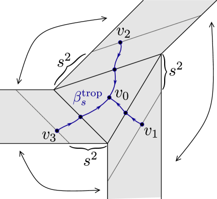
Figure 4.1. The tropical 1-cycle $\beta^{\text{trop}}_{s}$.

Along the path in $\beta_{s}^{\operatorname{trop}}$ connecting a one-valent vertex $v_{i}$ to $v_{0}$, we endow $\beta_{s,t}$ with the parallel transport of the primitive outward pointing vector $m=(1,0)$ in the asymptotic affine chart in Figure 3.3. The balancing condition at $v_{0}$ is

$$(1,1)+(-1,0)+(0,-1)=(0,0).$$

Thus $\beta_{s,t}$ with the edges oriented toward $v_{0}$ is a tropical $1$-chain in the sense of [RS], that is, a singular $1$-chain on the complement of the set of vertices of $B$ with values in the sheaf $\Lambda$ of integral tangent vectors.

The conormal construction of [RS, §2.3] now provides a singular $2$-chain $\beta_{s,0}$ in $\mathcal{X}_{0}$ with fibers $S^{1}$ over the interior of the edges of $\beta_{s}^{\operatorname{trop}}$ that contract to points at $\partial\sigma_{0}$, boundary three copies of $S^{1}$ in $w^{-1}(s)\cap\mathcal{X}_{0}$ and with a triangle inserted over $v_{0}$ to form a pair of pants. The property $\partial\beta_{s,t}\subset w^{-1}(s)$ holds because the edges of $\beta_{s}^{\operatorname{trop}}$ in the unbounded cells carry the asymptotic monomial.

Note that $w^{-1}(s)\cap\mathcal{X}_{0}$ is a union of three copies of $\mathbb{P}^{1}$ forming a cycle; indeed, the restriction of $\pi:\mathcal{X}\to\mathbb{C}$ to $w={\mathrm{const}}$ and $t$ sufficiently small is a base-changed Tate-curve, as is obvious from [CPS, Cor. 5.13]. Each of the three connected components of $\partial\beta_{s,0}$ splits one of the $\mathbb{P}^{1}\subset w^{-1}(s)\cap\mathcal{X}_{0}$ into two connected components.

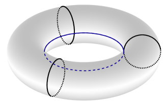
Figure 4.2. Sketch of $\partial\beta_{s,t}$ and $\partial\Gamma_{s,t}$ as three meridians and an equator in the elliptic curve $w^{-1}(s)\cap\mathcal{X}_{t}$.

The construction in [RS] also shows how $\beta_{s,0}$ extends to a continuous family $\beta_{s,t}$ of $2$-chains in $\mathcal{X}_{t}$, for $t$ in a contractible neighborhood in $\mathbb{C}^{*}$ of an interval $(0,t)$ with $t>0$ small. To treat the boundary, the construction allows to add the property

$$\partial\beta_{s,t}\subset w^{-1}(s).$$

The construction of $\beta_{s,t}$ can be extended to any contractible open set of $(s,t)\in\mathbb{C}^{*}\times\mathbb{C}$ such that $w^{-1}(s)\cap\mathcal{X}_{t}$ is not singular if $t\neq 0$, that is, with $\big{(}W(s,t)\big{)}^{3}\neq(3t)^{3}$. Figure 4.2 shows $\partial\beta_{s,t}$ and $\partial\Gamma_{s,t}$ as curves inside the elliptic curve $w^{-1}(s)\cap\mathcal{X}_{t}$.

The period integral $\Pi_{1}$ of $\Omega_{t}$ over $\beta_{s,t}$ can be readily computed by [RS]:

Proposition 4.2.

For any $s,t>0$ with $\beta_{s,t}$ defined we have

(4.7) $$\Pi_{1}(s,t)=\frac{1}{2\pi i}\int_{\beta_{s,t}}\Omega_{t}=\pi i+3(\log t-\log s).$$

Proof.

The integral follows from the computation in §3.6 of [RS], and notably Equation (3.17) with both the Ronkin function $\mathcal{R}$ and the gluing data $s_{\sigma,\underline{\rho}}$, $s_{\sigma^{\prime},\underline{\rho}}$ trivial. The integral thus becomes a sum over simple contributions from the vertices of $\beta^{\text{trop}}_{s}$. Up to the global factor ${2\pi i}$, the trivalent vertex contributes $\frac{1}{2}$, each bivalent vertex contributes $\log t$ and each univalent vertex contributes $-\log s$. ∎

The usual definition of a canonical coordinate now yields,

$$\exp\left(\frac{\Pi_{1}(s,t)}{\Pi_{0}(t)}\right)=\exp\big{(}\Pi_{1}(s,t)\big{)}=-t^{3}/s^{3}.$$

The first equality follows from the normalization property (4.3). Restricting to the distinguished fiber $s=1$ exhibits $-t^{3}$ as a canonical coordinate. But for fixed $t>0$, one could equally well view $s^{-3}$ as a canonical coordinate in the codomain of $W$.

As we will see in the proof of Proposition 4.7, the occurrence of the first summand $\pi i$ in $\Pi_{1}(s,t)$, which originates from the trivalent vertex of $\beta^{\operatorname{trop}}_{s,t}$, is our explanation for the negative sign in front of $q$ in (2.7).

A similar construction can be done in general. The resulting period integral gives different integral coefficients in Proposition 4.2, but due to the $\mathbb{C}^{*}$-action on the $\mathcal{X}$ acting with the same weights on $w$ and $t$ (Proposition 3.5) is always an affine function in $\log(t)-\log(s)$.

4.4. Main computation: Integration over positive real Lefschetz-thimbles

Our main result is the computation of the period integral

(4.8) $$\Pi_{2}(s,t)=\int_{\Gamma_{s,t}}\Omega_{t}$$

over the Lefschetz thimbles $\Gamma_{s,t}$ from (4.4) for cases such as the mirror family $\mathcal{X}$ of $(\mathcal{Y},\mathcal{D})$. We defined $\Gamma_{s,t}$ as a subset of the positive real locus $\mathcal{X}_{t}^{>}$, for $s,t\in\mathbb{R}_{>0}$ and $t/s$ small enough to fulfill $W(s,t)>3t$, the real critical value of $W$. Similarly to the family of $2$-chains $\beta_{s,t}$ in §4.3, there exists an extension of $\Gamma_{s,t}$ as a continuous family of $2$-chains not only to positive real $s,t$ with $t/s$ small, but to any contractible subset of $(s,t)\in(\mathbb{C}^{*})^{2}$ not containing a critical value of $W$ in the $(w,t)$-coordinates. In our computations, we nevertheless restrict to $s,t>0$ real and then argue by unique holomorphic continuation.

Note that for fixed $s$ the holomorphic continuation of the period integral $\Pi_{2}(s,t)$ about $t=0$ is multi-valued due to the log poles of $\Omega$ near the double locus of $\mathcal{X}_{0}$. Indeed, such period integrals, for $s$ fixed, may also involve constant multiples of $\log^{2}t$ and products of $\log t$ with a holomorphic function in $t$, as we explicitly saw in (2.5) in our review of Takahashi’s result.

Our computation works for any two-dimensional $\mathcal{X}$ obtained via [GHS] from a real wall structure on an asymptotically cylindrical integral affine manifold $B$ with integral polyhedral decomposition $\mathscr{P}$. The asymptotically cylindrical condition means that all unbounded edges in $\mathscr{P}$ are parallel [CPS, Def. 2.1]. Thus such a $B$ has asymptotic charts similar to the one shown in Figure 3.3. We also assume that all monomials in the slab and wall functions of unbounded walls are outgoing, meaning they are polynomials in $w^{-1}$, for $w$ as above the monomial with exponent the primitive outward pointing integral tangent vector of an unbounded edge. This assumption is automatically fulfilled by the wall structures from [GS22] or [GS11].

The complement of a compact subset $K\subset B$ is homeomorphic to $\mathbb{R}_{>0}\times S^{1}$, with polyhedral decomposition induced by a polyhedral decomposition of $S^{1}$ and the affine structure determined by two integers. These are the integral affine circumference $\ell\in\mathbb{N}\setminus\{0\}$ and $e\in\mathbb{Z}$ from the linear part of the affine monodromy $\left(\begin{smallmatrix}1&e\\ 0&1\end{smallmatrix}\right)$. We can thus write

(4.9) $$\textstyle B\setminus K\simeq\big{(}\mathbb{R}_{>0}\times[0,\ell]\big{)}\big{/}\sim,$$

where the equivalence relation identifies $\mathbb{R}_{>0}\times\{0\}$ and $\mathbb{R}_{>0}\times\{\ell\}$, and the inclusion of $\mathbb{R}_{>0}\times(0,\ell)$ is an affine isomorphism onto the image. In the case of our degeneration of $(\mathbb{P}^{2},E)$ we have $\ell=3$, $e=9$.

Non-horizontal walls in this asymptotic chart are bounded, see Figure 3.4. By working only with unbounded chambers to construct the $k$-th order smoothing $\mathcal{X}_{I}\setminus X_{\sigma_{0}}$ of $\mathcal{X}_{0}\setminus X_{\sigma_{0}}$, $I=(t^{k+1})$, we can thus restrict to unbounded, horizontal walls. For $k$ fixed we furthermore only consider the finite set of unbounded walls $\mathfrak{p}$ and slabs $\mathfrak{p}$ that are non-zero modulo $t^{k+1}$, as explained in §3.5. This finite wall-structure with all walls unbounded yields the same $\mathcal{X}_{I}\setminus X_{\sigma_{0}}$, which in turn agrees with the reduction modulo $t^{k+1}$ of the analytic family $\mathcal{X}\to\mathbb{C}$, restricted to the complement of $X_{\sigma_{0}}$. We label the slabs

$$\mathfrak{b}_{0},\ldots,\mathfrak{b}_{m}$$

cyclically from bottom to top in a diagram with the asymptotic direction horizontal to the right.

Denote further by

(4.10) $$\textstyle\kappa=\sum_{\rho}\kappa_{\rho}\in P=\mathbb{N}$$

the total kink of the multivalued piecewise linear function $\varphi$ entering the construction of [GHS] at infinity. In the canonical wall structure, $\kappa_{\rho}$ is the curve class associated to $\rho$. In our case we have $\kappa_{\rho}=3$ for all unbounded $\rho$, and $\kappa=3\cdot 3=9$.

The analytic function $w$ in §4.1 restricts to the unique monomial in

(4.11) $$S_{I}[\sigma_{\mathbb{Z}}^{\operatorname{gp}}]\simeq\mathbb{C}[t]/(t^{k+1})[w^{\pm 1},x^{\pm 1}]$$

of degree $0$ and associated tangent vector $(1,0)$. Noting that each wall function of an unbounded wall is a Laurent polynomial in $w^{-1}$ with coefficients in $\mathbb{C}[t]/(t^{k+1})$, we can then write

(4.12) $$f_{\mathrm{out}}=\prod_{\mathfrak{p}}f_{\mathfrak{p}}\cdot\prod_{\mathfrak{b}}f_{\mathfrak{b}}\in\mathbb{R}[t,w^{-1}]$$

with all $t$-exponents at most $k$ and $f_{\mathrm{out}}\equiv 1$ modulo $t$.

Since all these wall and slab functions have a non-zero constant coefficient, they have no zeros on any interval $[s_{0},\infty)$, $s_{0}>0$, as long as $t>0$ is sufficiently small. For $s_{1}>s_{0}>0$ and such $t$ we now define

$$\Gamma_{t}(s_{0},s_{1})=\mathcal{X}^{>0}\cap w^{-1}\big{(}[s_{0},s_{1}]).$$

Arguing with the degenerate momentum map $\mu:\mathcal{X}_{0}\to B$ as in §4.2, it is then not hard to see that $\Gamma_{t}(s_{0},s_{1})$ is a continuous family of cylinders. Moreover, letting $\delta$ be the integral affine distance function on $B$ from the union of bounded cells, $\mu$ identifies $\Gamma_{0}(s_{0},s_{1})$ with the annulus

$$\delta^{-1}\big{(}[s_{0}^{2},s_{1}^{2}]\big{)}$$

in $B$. Indeed, by our definition of $\mu$, the value of $|w|$ on $\mu^{-1}(a)$ equals $a^{1/2}$. Note also that if there exists a positive real Lefschetz thimble $L_{s,t}$, as in the case of the mirror of $(\mathcal{Y},\mathcal{D})$ from §3.1, then

$$\Gamma_{t}(s_{0},s_{1})=\Gamma_{s_{1},t}-\Gamma_{s_{0},t}$$

as a singular chain.

After requiring the monomial for $w$ to be given by $(1,0)$, the asymptotic affine chart induced from (4.9) becomes unique up to an affine transformation with an integral translation and linear part $\left(\begin{smallmatrix}1&k\\ 0&1\end{smallmatrix}\right)$ for $k\in\mathbb{Z}$. We fix one such choice together with a choice of slab $\mathfrak{b}_{0}$ to function as a radial cut. Parallel transport of the basis vector $(0,1)$ on the contractible set $B\setminus\mathfrak{b}_{0}$ now provides us with a choice of monomials $u,v$ in each model ring $R_{\mathfrak{b}_{i}}^{I}$ from (3.10). The $u,v$ generize to monomials with opposite tangent vectors in $S_{I}[\sigma^{\operatorname{gp}}_{\mathbb{Z}}]$, which for $i\neq 0$ we can take to be $x,x^{-1}$ in (4.11). For $i=0$ we take $u=x$ and then $v=x^{-1}w^{-e}$ due to the affine monodromy. Note also that these $(\operatorname{Spec}R_{\mathfrak{b}_{i}})_{\mathrm{an}}$ cover $\mathcal{X}_{I}\setminus X_{\sigma_{0}}$ since each other type of model ring $S_{I}[\sigma_{\mathbb{Z}}^{\operatorname{gp}}]$ is obtained by a sequence of localizations (3.11), (3.12) and isomorphisms (3.8).

Let $u_{i}$ be an analytic extension of $u\in R_{\mathfrak{b}_{i}}$ to an open subset $U_{i}\subset\mathcal{X}$, compatible with the real structure and such that

$$\Omega_{t}=\operatorname{dlog}w\wedge\operatorname{dlog}u_{i}$$

holds locally. Since $v=f_{\mathfrak{b}_{i}}\cdot t^{\kappa_{i}}/u$ in $R_{\mathfrak{b}_{i}}$, the same formula with $u$ replaced by $u_{i}$ defines an analytic function $v_{i}$ on $U_{i}$ with

(4.13) $$u_{i}v_{i}=f_{\mathfrak{b}_{i}}(w,t)\cdot t^{\kappa_{i}}.$$

We are now ready for the main period computation.

Proposition 4.3.

For $s_{1}>s_{0}>0$, and $t>0$ sufficiently small we have

$$\int_{\Gamma_{t}(s_{0},s_{1})}\Omega_{t}=-\int_{s_{0}}^{s_{1}}\Big{(}\log t^{\kappa}-\log s^{e}+\log f_{\mathrm{out}}(s,t)\Big{)}\operatorname{dlog}s+O(t^{k+1}).$$

Proof.

The integral is real analytic in $s_{0},s_{1}$. By analytic continuation it therefore suffices to prove the result for $s_{0},s_{1}\gg 0$.

Since the $U_{i}$ cover $\mathcal{X}_{0}\setminus X_{\sigma_{0}}$ the $U_{i}$ cover $\Gamma_{t}(s_{0},s_{1})$ for sufficiently small $t>0$. Moreover, $(w,u_{i})$ or $(w,v_{i})$ from above provide real, oriented coordinate systems on $\Gamma_{t}(s_{0},s_{1})\cap U_{i}$. By (4.13) we can also impose the condition $v_{i}\leq 1$, or equivalently

(4.14) $$u_{i}\geq f_{\mathfrak{b}_{i}}(w,t)\cdot t^{\kappa_{i}}$$

on $U_{i}$ and still cover $\Gamma_{t}(s_{0},s_{1})$ for small $t$.

Noting that the $U_{i}\cap U_{i+1}$ with $U_{m+1}=U_{0}$ cover all but the double locus of $\mathcal{X}_{0}\setminus X_{\sigma_{0}}$, the $U_{i}\cap U_{i+1}$ also cover $\Gamma_{t}(s_{0},s_{1})$ for $t$ sufficiently small. Denote by $\mathfrak{P}_{i}$ the set of walls between the slabs $\mathfrak{b}_{i}$ and $\mathfrak{b}_{i+1}$. Then on $U_{i}\cap U_{i+1}$, $i=0,\ldots,m-1$, the wall crossing automorphisms (3.9) provide the relation

(4.15) $$\textstyle u_{i}\cdot v_{i+1}=f_{i}(w,t)^{-1},\quad f_{i}\equiv\prod_{\mathfrak{p}\in\mathfrak{P}_{i}}f_{\mathfrak{p}}\,\mod t^{k+1}.$$

The inverse comes from the fact that the exponents for $u_{i}$ and $v_{i+1}$ both point into the walls rather than away, in contrast to $u_{i},v_{i}$ in the slab relation (4.13). Thus $v_{i+1}\geq 1$ if and only if

(4.16) $$u_{i}\leq f_{i}(w,t)^{-1}.$$

For $i=m$ the monodromy brings in an additional factor $w^{-e}$ and (4.15) holds with

(4.17) $$\textstyle f_{0}\equiv w^{-e}\cdot\prod_{\mathfrak{p}\in\mathfrak{P}_{0}}f_{\mathfrak{p}}\,\mod t^{k+1}.$$

The inequalities (4.14), (4.16) now provide a decomposition of $\Gamma_{t}(s_{0},s_{1})$ for $t>0$ small into the domains

$$s_{0}\leq w\leq s_{1},\quad f_{\mathfrak{b}_{i}}(w,t)\cdot t^{\kappa_{i}}\leq u_{i}\leq f_{i}(w,t)^{-1},$$

a subset of $U_{i}$, $i=0,\ldots,m$.

We obtain

(4.18) $$\int_{\Gamma_{t}(s_{0},s_{1})}\Omega_{t} =\sum_{i=0}^{m}\int_{s_{0}}^{s_{1}}\left(\int_{f_{\mathfrak{b}_{i}}(w,t)\cdot t^{\kappa_{i}}}^{f_{i}^{-1}(w,t)}\operatorname{dlog}u_{i}\right)\operatorname{dlog}w$$

$$=-\sum_{i=0}^{m}\int_{s_{0}}^{s_{1}}\Big{(}\log(t^{\kappa_{i}})+\log f_{\mathfrak{b}_{i}}(w,t)+\log f_{i}(w,t)\Big{)}\operatorname{dlog}w$$

$$=-\int_{s_{0}}^{s_{1}}\Big{[}\log t^{\kappa}-\log w^{e}+\log f_{\mathrm{out}}(w,t)\Big{]}\operatorname{dlog}w+O(t^{k+1}).$$

The last equality uses $\kappa=\sum_{i}\kappa_{i}$ from (4.10) and the definitions of $f_{\mathrm{out}}$ and $f_{i}$ in (4.12), (4.15), (4.17). ∎

Remark 4.4.

For an alternative proof of Proposition 4.3, we could have used [CPS, Constr. 5.5] of an asymptotic polyhedral affine pseudomanifold with asymptotic wall structure that includes walls with reduction modulo $t$ a constant different from $1$, along with [RS]. The computation then still reduces to an integral over a degenerating family of elliptic curves.

We are now ready to prove our main result. Recall that by [GS22, (3.11)] or [Gr20, Thm. 2], the infinite product of all asymptotic wall functions is given by

(4.19) $$\log f_{\mathrm{out}}(w,t)=\sum_{d=1}^{\infty}\,3d\,N_{d}\,w^{-3d}\,t^{3d}.$$

Theorem 4.5.

Let $\mathcal{X}\to\mathbb{C}$ be the analytic intrinsic mirror of our maximal degeneration $(\mathcal{Y},\mathcal{D})\to\mathbb{A}^{1}$ of $(\mathbb{P}^{2},E)$ and $\Gamma_{s,t}$ the positive real Lefschetz thimble from (4.4) with boundary on $w=s$. Then

$$t\partial_{t}\,\Pi_{2}(s,t)=t\partial_{t}\int_{\Gamma_{s,t}}\Omega=9\log(t/s)+\sum_{d\geq 1}3dN_{d}(t/s)^{3d}.$$

Proof.

The $\mathbb{C}^{*}$-action on $\mathcal{X}$ of Proposition 3.5 implies that for all $\lambda\in\mathbb{C}^{*}$,

$$\Gamma_{\lambda s,\lambda t}=\lambda\cdot\Gamma_{s,t}.$$

Here the multiplication by $\lambda$ on the right-hand side denotes the action. Since $\lambda^{*}\Omega_{\lambda t}=\Omega_{t}$, we obtain

$$\Pi_{2}(\lambda s,\lambda t)=\int_{\Gamma_{\lambda s,\lambda t}}\Omega_{\lambda t}=\int_{\Gamma_{s,t}}\Omega_{t}=\Pi_{2}(s,t).$$

Taking the derivative with respect to $\lambda$ at $\lambda=1$ thus shows

$$t\partial_{t}\int_{\Gamma_{s,t}}\Omega=-s\partial_{s}\int_{\Gamma_{s,t}}\Omega.$$

Now $\Omega$ is closed for $t={\mathrm{const}}$, hence exact along the contractible $2$-chain $\Gamma_{s,t}$. Thus by Stokes’ Theorem,

$$s\partial_{s}\,\Pi_{2}(s,t)=s\partial_{s}\int_{\Gamma_{t}(s_{0},s)}\Omega$$

for $s_{0}<s$ sufficiently close to $s$. The right-hand side can readily be computed from Proposition 4.3 while taking the limit $k\to\infty$ to give

$$t\partial_{t}\,\Pi_{2}(s,t)=-s\partial_{s}\int_{\Gamma_{t}(s_{0},s)}\Omega=\log t^{\kappa}-\log s^{e}+\log f_{\mathrm{out}}(s,t).$$

Noting that $\kappa=e=9$ and plugging in (4.19) gives the stated formula. ∎

Proof of Theorem 1.1. The statement follows from Theorem 4.5 by setting $s=1$ and integration. ∎

Remark 4.6.

In higher dimensions, an analogous period computation can be done for the intrinsic mirror of a normal crossing degeneration $(\mathcal{Y},\mathcal{D})$ of a Fano manifold $Y$ with smooth anticanonical divisor $D$. The positive real locus in that case has to be replaced by a real one-parameter family of cycles induced by a tropical $1$-cycle as in [RS] in the asymptotic singular affine manifold $B_{\infty}$ from [CPS, Constr. 5.5]. At least in the case that this asymptotic tropical $1$-cycle is the tropicalization of a family of curves $\mathcal{C}\subset\mathcal{D}$, we expect the period integral computes the generating function of logarithmic Gromov-Witten invariants in $Y$ intersecting $D$ only in a point of $C=\mathcal{C}\cap Y$.

4.5. Corollary: Takahashi’s log mirror symmetry conjecture

To deduce Takahashi’s enumerative mirror conjecture (2.7) from our periods, we simply observe that in the canonical coordinate $q=-e^{I_{1}(Q)}$, Takahashi’s basis $I_{0}(Q)$, $I_{1}(Q)$, $I_{2}(Q)$ of solutions of the Picard-Fuchs equation is the unique tuple of solutions obeying

$$I_{0}(q) =1$$

$$I_{1}(q) =\log q$$

$$I_{2}(q) =\frac{1}{2}\log^{2}q+I_{2}^{\mathrm{hol}}(q).$$

Proposition 4.7.

The periods $\Pi_{1}(t),\Pi_{1}(s,t),\Pi_{2}(s,t)$ from (4.3), (4.7), (4.8) at $s=1$ fulfill

$$I_{0}(-t^{3}) =\Pi_{0}(t)=1$$

$$I_{1}(-t^{3}) =\Pi_{1}(1,t)=3\log t$$

$$I_{2}(-t^{3}) =\Pi_{2}(1,t)+c.$$

for some $c\in\mathbb{R}$.

Proof.

The first equality is (4.3). The second equality follows from (4.2) by

$$-\exp\big{(}\Pi_{1}(1,t)\big{)}=-\exp\big{(}\pi i+3\log t\big{)}=t^{3}$$

and the definition of $q$. Finally, Theorem 1.1 shows that $\Pi_{2}(1,t)$ and $I_{2}(-t^{3})$ are both solutions of the Picard-Fuchs equation (2.4) with the same coefficient of $\log^{2}(t)$, namely $1/2$. Since the space of solutions with non-zero $\log^{2}(t)$-term and vanishing $\log(t)$- and constant terms is one-dimensional, we obtain the third equality. ∎

Corollary 4.8.

Takahashi’s enumerative mirror conjecture (2.7) holds up to an additive constant.

Proof.

The statement follows readily from Proposition 4.7 and Theorem 1.1. ∎

References

- [AGIS] M. Abouzaid, S. Ganatra, H. Iritani, N. Sheridan: The Gamma and Strominger-Yau-Zaslow conjectures: A tropical approach to periods, Geom. Topol. 24 (2020), 2547–2602.
- [AC] D. Abramovich, Q. Chen: Stable logarithmic maps to Deligne-Faltings pairs. II, Asian J. Math. 18 (2014), 465–488.
- [ACGS] D. Abramovich, Q. Chen, M. Gross, B. Siebert: Punctured logarithmic maps, Mem. Eur. Math. Soc. 15, 2024.
- [A] H. Argüz: Real loci in (log) Calabi-Yau manifolds via Kato-Nakayama spaces of toric degenerations, Eur. J. Math. 7 (2021), 869–930.
- [AKV] M. Aganagic, A. Klemm, C. Vafa: Disk instantons, mirror Symmetry and the duality web, Z. Naturforsch. A 57 (2002), 1–28.
- [AV] M. Aganagic, C. Vafa: Mirror Symmetry, D-Branes and Counting Holomorphic Discs, arXiv:hep-th/0012041 (2000).
- [AD] M. Artebani, I. Dolgachev: The Hesse pencil of plane cubic curves, Enseign. Math. 55 (2009), 235–273.
- [B] V. Batyrev: Dual polyhedra and mirror symmetry for Calabi-Yau hypersurfaces in toric varieties, J. Algebr. Geom. 3, (1994) 493–535.
- [BB] V. Batyrev, L. Borisov: Mirror duality and string-theoretic Hodge numbers, Invent. Math. 126 (1996), 183–203.
- [BH] P. Berglund, T. Hübsch: A generalized construction of mirror manifolds, Nuclear Phys. B393 (1993), 377–391.
- [B20] P. Bousseau: The quantum tropical vertex, Geom. Topol. 24 (2020), 1297–1379.
- [B22] P. Bousseau: Scattering diagrams, stability conditions, and coherent sheaves on , J. Algebraic Geom. 31 (2022), 593–686.
- [B23] P. Bousseau: A proof of N. Takahashi’s conjecture for and a refined sheaves/Gromov-Witten correspondence Duke Math. J. 172 (2023), 2895–2955.
- [BBvG] P. Bousseau, A. Brini, M. van Garrel: Stable maps to Looijenga pairs, Geom. Topol. 28 (2024), no. 1, 393–496.
- [BS] A. Brini, Y. Schuler: Refined Gromov-Witten invariants, arXiv:2410.00118.
- [CLS] P. Candelas, M. Lynker, R. Schimmrigk: Calabi-Yau manifolds in weighted , Nuclear Phys. B341 (1990), 383–402.
- [CPS] M. Carl, M. Pumperla, B. Siebert: A tropical view on Landau-Ginzburg models, Acta Math. Sin. (Engl. Ser.) 40 (2024), 329–382.
- [CLL] K. Chan, S.-C. Lau, N. C. Leung: SYZ mirror symmetry for toric Calabi-Yau manifolds, J. Differential Geom. 90 (2012), no. 2, 177–250.
- [CLT] K. Chan, S.-C. Lau, H.-H. Tseng: Enumerative meaning of mirror maps for toric Calabi-Yau manifolds, Adv. Math. 244 (2013), 605–625.
- [Ch] Q. Chen: Stable logarithmic maps to Deligne-Faltings pairs I, Ann. Math. (2) 180, No. 2, 455–521 (2014).
- [CKYZ] T.-M. Chiang, A. Klemm, S.-T. Yau, E. Zaslow: Local mirror symmetry: Calculations and interpretations, Adv. Theor. Math. Phys. 3, No. 3, 495–565 (1999).
- [CdOGP] P. Candelas, X. de la Ossa, P. Green, L. Parkes, A pair of Calabi–Yau manifolds as an exactly soluble superconformal theory, Nucl. Phys. B359 (1991), 21–74.
- [CvGKT] J. Choi, M. van Garrel, S. Katz, N. Takahashi: Log BPS numbers of log Calabi–Yau surfaces, Trans. Am. Math. Soc. 374 (2021), 687–732.
- [FTY] H. Fan, H.-H. Tseng, F. You: Mirror Theorems for Root Stacks and Relative Pairs, Sel. Math., New Ser. 25 (4) (2019), Paper No. 6, 33pp.
- [GP] S. Ganatra, D. Pomerleano: Symplectic cohomology rings of affine varieties in the topological limit, Geom. Funct. Anal. 30 (2020), 334–456.
- [vGGR] M. van Garrel, T. Graber, H. Ruddat: Local Gromov-Witten invariants are log invariants, Adv. Math. 350 (2019), 860–876.
- [vGNS] M. van Garrel, N. Nabijou, Y. Schuler: Gromov-Witten theory of bicyclic pairs, arXiv:2310.06058.
- [Ga] A. Gathmann: Relative Gromov–Witten invariants and the mirror formula, Math. Ann. 325 (2003), 393–412.
- [GZ] T. Graber, E. Zaslow, Open-string Gromov-Witten invariants: calculations and a mirror “theorem”, in: Orbifolds in mathematics and physics (Madison, WI, 2001), Contemp. Math. 310, AMS 2002, 107–121.
- [Gr20] T. Gräfnitz: Tropical correspondence for smooth del Pezzo log Calabi-Yau pairs, J. Algebraic Geom. 31 (2022), 687–749.
- [Gr21] T. Gräfnitz: Sage code to compute scattering diagrams, available at https://timgraefnitz.com/.
- [Gr22a] T. Gräfnitz: Theta functions, broken lines and 2-marked log Gromov-Witten invariants, arXiv:2204.12257.
- [GRZ] T. Gräfnitz, H. Ruddat, E. Zaslow: The proper Landau-Ginzburg potential is the open mirror map, Adv. Math. 447 (2024).
- [GRZZ] T. Gräfnitz, H. Ruddat, E. Zaslow, Benjamin Zhou: Enumerative Geometry of Quantum Periods, arXiv:2502.19408.
- [GrPl] B. Greene and M. Plesser: Duality in Calabi-Yau moduli space, Nuclear Phys. B 338 (1990), 15–37.
- [Gro] M. Gross: Examples of special Lagrangian fibrations, in: Symplectic geometry and mirror symmetry (Seoul, 2000), 81–109, World Sci. Publ., River Edge, NJ.
- [GHK] M. Gross, P. Hacking, Paul, S. Keel: Mirror symmetry for log Calabi-Yau surfaces. I, Publ. Math., Inst. Hautes Étud. Sci. 122, 65-168 (2015).
- [GHS] M. Gross, P. Hacking, B. Siebert: Theta functions on varieties with effective anti-canonical class, Memoirs of the American Mathematical Society 1367. AMS 2022.
- [GPS] M. Gross, R. Pandharipande, B. Siebert: The tropical vertex, Duke Math. J. 153 (2) (2010), 297–362.
- [GS11] M. Gross, B. Siebert: From real affine geometry to complex geometry, Ann. Math. (2) 174, No. 3, 1301–1428 (2011).
- [GS13] M. Gross, B. Siebert: Logarithmic Gromov-Witten invariants, J. Am. Math. Soc. 26, No. 2, 451–510 (2013).
- [GS14] M. Gross, B. Siebert: Local mirror symmetry in the tropics, Proceedings of the International Congress of Mathematicians (ICM 2014), Seoul, Korea.
- [GS18] M. Gross, B. Siebert: Intrinsic mirror symmetry and punctured Gromov-Witten invariants, Algebraic geometry: Salt Lake City 2015, 199–230. Proc. Sympos. Pure Math., 97.2, AMS, Providence, RI, 2018.
- [GS19] M. Gross, B. Siebert: Intrinsic Mirror Symmetry, arXiv:1909.07649.
- [GS22] M. Gross, B. Siebert: The canonical wall structure and intrinsic mirror symmetry, Invent. Math. 229, No. 3, 1101–1202 (2022).
- [I] H. Iritani, Mirror symmetric Gamma conjecture for Fano and Calabi-Yau manifolds, arXiv:2307.15940.
- [J] S. Johnston: Comparison of non-archimedean and logarithmic mirror constructions via the Frobenius structure theorem, arXiv:2204.00940.
- [KKMS] G. Kempf, F. Knudsen, D. Mumford, B. Saint-Donat: Toroidal Embeddings I, Springer, LNM 339, 1973.
- [KY23] S. Keel, T. Yu: The Frobenius structure theorem for affine log Calabi-Yau varieties containing a torus, Ann. of Math.198 (2023), 419–536.
- [KY24] S. Keel, T. Yu: Log Calabi-Yau mirror symmetry and non-archimedean disks, arXiv:2411.04067.
- [L] S.-C. Lau, Gross-Siebert’s slab functions and open GW invariants for toric Calabi-Yau manifolds, Math. Res. Lett. 22, No. 3, 881–898 (2015).
- [RS] H. Ruddat, B. Siebert: Period integrals from wall structures via tropical cycles, canonical coordinates in mirror symmetry and analyticity of toric degenerations, Publ. Math. Inst. Hautes Études Sci. 132 (2020), 1–82.
- [Se] P. Seidel: A biased view of symplectic cohomology, Current developments in mathematics, 2006, 211–253, Int. Press 2008.
- [T96] N. Takahashi: Curves in the complement of a smooth plane cubic whose normalizations are , arXiv:alg-geom/9605007.
- [T01] N. Takahashi: Log mirror symmetry and local mirror symmetry, Comm. Math. Phys. 220 (2) (2001), 293–299.
- [TY] H.-H. Tseng, F. You: A mirror theorem for multi-root stacks and applications, Sel. Math. New Ser. 29, 6 (2023).
- [W] Y. Wang: Gross–Siebert intrinsic mirror ring for smooth log Calabi–Yau pairs, arXiv:2209.15365.
- [Y] F. You: The proper Landau–Ginzburg potential, intrinsic mirror symmetry and the relative mirror map, Commun. Math. Phys. 405, Paper No. 79, 44pp. (2024).