Synaptic shot-noise triggers fast and slow global oscillations
in balanced neural networks

Abstract

Neural dynamics is determined by the transmission of discrete synaptic pulses (synaptic shot-noise) among neurons. However, the neural responses are usually obtained within the diffusion approximation modeling synaptic inputs as continuous Gaussian noise. Here, we present a rigorous mean-field theory that encompasses synaptic shot-noise for sparse balanced inhibitory neural networks driven by an excitatory drive. Our theory predicts new dynamical regimes, in agreement with numerical simulations, which are not captured by the classical diffusion approximation. Notably, these regimes feature self-sustained global oscillations emerging at low connectivity (in-degree) via either continuous or hysteretic transitions and characterized by irregular neural activity, as expected for balanced dynamics. For sufficiently weak (strong) excitatory drive (inhibitory feedback) the transition line displays a peculiar re-entrant shape revealing the existence of global oscillations at low and high in-degrees, separated by an asynchronous regime at intermediate levels of connectivity. The mechanisms leading to the emergence of these global oscillations are distinct: drift-driven at high connectivity and cluster activation at low connectivity. The frequency of these two kinds of global oscillations can be varied from slow ($\sim 1$ Hz) to fast ($\sim 100$ Hz), without altering their microscopic and macroscopic features, by adjusting the excitatory drive and the synaptic inhibition strength in a prescribed way. Furthermore, the cluster-activated oscillations at low in-degrees could correspond to the $\gamma$ rhythms reported in mammalian cortex and hippocampus and attributed to ensembles of inhibitory neurons sharing few synaptic connections [G. Buzsáki and X.-J. Wang, Annual Review of Neuroscience 35, 203 (2012)].

I Introduction

Shot-noise (or Poissonian noise) is a model of discontinuous noise characterized by a sequence of discrete pulses occurring at Poisson-distributed times. It is a ubiquitous process in Nature, observable in electrical circuits and in optics due to the discrete nature of charges and photons Schottky (1918); Henry and Kazarinov (1996), as well as in population dynamics due to the discreteness of individuals Goncalves et al. (2023). Furthermore, the inclusion of shot-noise is fundamental to fully characterize the considered phenomena in many fields of physics ranging from granular systems Kanazawa (2017); Lucente et al. (2023, 2025) to active matter Fodor et al. (2018), and from mesoscopic conductors Blanter and Büttiker (2000) to Anderson localization Frisch and Lloyd (1960).

Neural dynamics is also intimately linked to the discrete nature of the synaptic events (post-synaptic potentials (PSPs)) regulating the firing activity of the neurons. In the cortex, the PSPs received by a neuron are usually assumed to be of small amplitude and to have high arrival rates, due to the high number of pre-synaptic connections. Furthermore, since the number of pre-synaptic neurons is small with respect to the large number of neurons present in the cortex, the PSPs stimulating a specific neuron are assumed to be uncorrelated. Therefore, the synaptic inputs have been usually treated as white noise (as a continuous Gaussian process) giving rise to the so-called Diffusion Approximation (DA) for the mean-field description of the neural dynamics Capocelli and Ricciardi (1971); Tuckwell (1988).

However, experimental results challenge the hypotheses at the basis of the DA. First of all, there is clear evidence that synaptic weight distributions display heavy tails towards large values Miles (1990); Song et al. (2005); Buzsáki and Mizuseki (2014). Moreover, rare large-amplitude synaptic connections are likely to contribute strongly to reliable information processing Lefort et al. (2009) and the synaptic weight distributions can be deeply modified by plasticity during learning processes and ongoing activity Bi and Poo (1999); Barbour et al. (2007). A second important aspect is that neural circuits can display a connectivity definitely lower than expected. Indeed, networks of inhibitory neurons with very low number of pre-synaptic connections (in-degree $K\simeq 30-80$) have been found in the cat visual cortex Kisvárday et al. (1993) and in the rat hippocampus Sik et al. (1995), the latter population of interneurons is believed to be responsible for the emergence of global oscillations (GOs) in the $\gamma$-band ($30-100$ Hz) Buzsáki and Wang (2012). Along this direction goes a recent study reporting that primate excitatory and inhibitory neurons receive 2-5 times fewer excitatory and inhibitory synapses than similar mouse neurons Wildenberg et al. (2021).

These experimental indications call for the investigation of the dynamical regimes emerging in highly diluted neural networks under the effect of synaptic shot-noise. Several works have been devoted to the development of mean-field approaches describing the population dynamics of Integrate-and-Fire neurons subject to synaptic shot-noise, though mostly focused on asynchronous regimes Richardson and Swarbrick (2010); Iyer et al. (2013); Olmi et al. (2017); Angulo-Garcia et al. (2017); Droste and Lindner (2017); Richardson (2018, 2024).

However, oscillations are extremely relevant for the brain functioning, since they play a fundamental role in orchestrating cognitive functions and are often disrupted in neurological disorders Buzsaki (2006); Singer (2018). Oscillations in the brain are typically characterized by irregular neural firing, where neurons fire at frequencies much lower than those of the GOs both in vivo Csicsvari et al. (1998) and in in vitro Fisahn et al. (1998). Several works have shown that this type of oscillations can arise in balanced excitatory-inhibitory sparse networks van Vreeswijk and Sompolinsky (1996), due to the interplay between endogenous fluctuations and neural coupling Brunel (2000); Brunel and Wang (2003); Geisler et al. (2005); Bi et al. (2021). In particular, inhibition has been shown to play a critical role for the emergence of GOs, both in experimental data and in neural network models Whittington et al. (2000); Mann and Paulsen (2007). Therefore, GOs have often been analyzed within the simplified context of purely inhibitory networks, where the balance occurs between an external excitatory drive and the recurrent inhibition Brunel and Hakim (1999); Kadmon and Sompolinsky (2015); Monteforte and Wolf (2010); di Volo and Torcini (2018); Di Volo et al. (2022). The characterization of the dynamical regimes exhibited by these models has been usually performed at a mean-field level within the context of the DA Brunel and Hakim (1999); Brunel (2000). Only quite recently, some of the authors of this article have introduced in Goldobin et al. (2024) a mean-field approach incorporating shot-noise and sparsity in the connectivity to describe the emergence of GOs in balanced inhibitory neural networks.

In the present paper, we report in details the derivation of the complete mean-field approach (CMF) introduced in Goldobin et al. (2024) for the Quadratic Integrate-and-Fire (QIF) neurons Ermentrout and Kopell (1986); Gutkin (2022). Furthermore, we will extend the analysis in Goldobin et al. (2024) to the derivation of the diffusion (DA) and third order approximation (D3A), obtained by expanding the source term in the continuity equation to the second and third order, respectively. A weakly non-linear analysis of the stationary solutions displayed by the CMF allows to identify hysteretic and non-hysteretic transitions towards GOs with associated region of coexistence of GOs and asynchronous states. These forecasts are in good agreement with accurate numerical simulations, as shown via finite size analysis of the observed transitions. On the other hand, DA and D3A fail in reproducing the network dynamics for sufficiently low excitatory drive (high inhibitory feedback). A peculiarity of the bifurcation diagram found with the CMF approach is a re-entrant Hopf bifurcation line separating GOs observable at low and large in-degree $K$ from asynchronous irregular regime at intermediate $K$. These two kinds of GOs, induced by synaptic shot-noise, are characterized, as the intermediate asynchronous state, by neurons spiking irregularly, but they emerge due to two different mechanisms. Moreover, both types of GOs can be observed at low frequencies (in the $\delta$-band ($0.5-3.5$ Hz)) and at high frequencies (in the $\gamma$-band) by properly rescaling the external excitatory drive and the inhibitory synaptic strength, while the mean frequency of the irregularly firing neurons is always definitely slower.

The paper is organized as follows. Section II is devoted to the introduction of the network model, of the simulation protocols and of the indicators employed to characterize microscopic and macroscopic dynamics. The mean-field formulation of the model is reported in Section III. In particular, we derive the macroscopic evolution equations for the CMF, the diffusion and third order approximation, together with the corresponding linear and weakly non-linear stability analysis of the asynchronous regime. The mean-field results are compared with network simulations in Sect. IV. This section reports a characterization of the observed transitions and macroscopic regimes, as well as the explanation of the two mechanisms that are at the origin of the two classes of GOs, induced by discrete synaptic events, observable at small and large in-degree. A summary and discussion of the results can be found in Sect. V. A detailed presentation of the integration methods employed for the network model and for the Langevin and continuity equations can be found in Appendix A-C. Finally Appendix D compares the results for the macroscopic dynamics obtained by network simulations and mean-field analysis for non-instantaneous synapses.

II Model and Methods

II.1 The Network Model

As a prototype of a dynamically balanced system we consider a sparse inhibitory network made of $N$ pulse-coupled QIF neurons Monteforte and Wolf (2010); di Volo and Torcini (2018); Di Volo et al. (2022) whose membrane potentials evolve according to the equations

$$\dot{v}_{i}(t)=v_{i}^{2}+I-g\sum_{j=1}^{N}\sum_{n}\varepsilon_{ji}\delta(t-t_{j}^{(n)})\quad v\in]-\infty,+\infty[;$$ (1)

where $I$ represents an external DC current, $g$ the synaptic coupling, and the last term on the rhs the inhibitory synaptic current. The latter is the linear superposition of instantaneous inhibitory PSPs emitted at times $t_{j}^{(n)}$ from the pre-synaptic neurons connected to neuron $i$. $\varepsilon_{ji}$ is the adjacency matrix of the random network with entries $1$ $(0)$ if the connection from node $j$ to $i$ exists (or not), and we assume the same in-degree $K=\sum_{j}\varepsilon_{ji}$ for all neurons.

We consider the quadratic integrate-and-fire (QIF) neuron Ermentrout and Kopell (1986), which is a current-based model of class I excitability. In particular, whenever the membrane potential ${v}$ reaches infinity, a $\delta$-spike is emitted and instantaneously delivered to the post-synaptic neurons and ${v}$ is reset to $-\infty$. In the absence of synaptic coupling, the QIF model displays excitable (oscillatory) dynamics for $I<0$ ($I>0$). Since we consider a purely inhibitory network in order to have non-trivial collective dynamics the neurons should be supra-threshold, i.e. with $I>0$, in this case in absence of synaptic coupling the single neuron firing frequency is given by

$$\nu_{0}=\frac{\sqrt{I}}{\pi}=\frac{1}{T_{0}}$$ (2)

In the excitable case ($I<0$) the neuron has a stable and an unstable fixed points located at $V^{s}=-\sqrt{-I}$ and $V^{u}=\sqrt{-I}$, respectively.

The DC current and the synaptic coupling are assumed to scale as $I=i_{0}\sqrt{K}$ and $g=g_{0}/\sqrt{K}$ as usually done in order to ensure a self-sustained balanced state for sufficiently large $K$ van Vreeswijk and Sompolinsky (1996); Monteforte and Wolf (2010); di Volo and Torcini (2018).

The times (frequencies) are reported in physical units by assuming as a time scale a membrane time constant $\tau_{m}=10$ ms.

II.2 Simulation Protocols

The simulation of the QIF network model (1) has been performed thanks to an exact event-driven method (see Appendix A for more details), this allowed us to reach very large system sizes from $N=10000$ up to $N=80000$ with $10\leq K\leq 1000$, to integrate for long time spans up to $50-100$ secs and to average over 5-20 different network realizations.

The simulations performed to identify the emergence of collective oscillations are usually based on two quasi-adiabatic protocols, where $i_{0}$ ($K$) is varied in steps $\Delta i_{0}$ ($\Delta_{K}$) by maintaning all the other parameters constant. The simulations are performed for some value of $i_{0}$ ($K$) where the quantities of interest are evaluted over a certain time interval $t_{E}\simeq 20-30$ s after discarding a transient of durations $t_{T}\simeq 20-30$ s. At the end of the simulation the final values of the variables are stored and used to initialize the next simulation step with a parameter value $i_{0}\pm\Delta i_{0}$ ($K\pm\Delta K$), whose duration will be again $t_{T}+t_{E}$. These steps are repeated until the final parameter value is achieved, to test for hysteresis the procedure can be reversed by decreasing (increasing) the parameter value in small steps to recover the initial value.

II.3 Indicators

The microscopic evolution of the neurons is typically measured in terms of the mean inter-spike interval (ISI) of each neuron $\langle T_{i}\rangle$ and of the corresponding firing rate $\nu_{i}=1/\langle T_{i}\rangle$, where $\langle\cdot\rangle$ denotes a time average. The neural variability of each neuron is customarily measured via the so-called coefficient of variation

$$cv_{i}=\frac{\sqrt{\langle T^{2}_{i}\rangle-\langle T_{i}\rangle^{2}}}{\langle T_{i}\rangle}$$

which is the ratio between the standard deviation and the mean of the ISIs of the neuron $i$. A value $cv_{i}=0$ ($cv_{i}=1$) corresponds to a periodic (Poissonian) activity of the considered neuron Tuckwell (1988).

The activity of the neurons in the network can be therefore characterized in terms of the ensemble averages of the firing rates ${F}=\overline{\nu_{i}}=\frac{1}{N}\sum_{i=1}^{N}\nu_{i}$, of the coefficient of variations $CV=\overline{cv_{i}}$ and of the corresponding probability distribution functions PDFs.

The population activity can be also analyzed in terms of the population firing rate $\nu(t)$

$$\nu(t)=\frac{N_{sp}(T_{W})}{T_{W}N}\quad.$$ (3)

where $N_{sp}(T_{W})$ is the number of spikes emitted by the $N$ neurons in the network in a time interval $T_{W}$, which we typically consider of the order of $0.005$.

The macroscopic evolution of the network can be characterized by the indicator introduced in Golomb (2007)

$$\rho=\left(\frac{\sigma^{2}_{V}}{\overline{\sigma_{i}^{2}}}\right)^{1/2}\quad{\rm where}\quad\sigma_{i}^{2}=\langle v_{i}^{2}\rangle-\langle v_{i}\rangle^{2}\quad$$ (4)

and $\sigma_{V}$ is the standard deviation of the mean membrane potential $V(t)=\overline{v_{i}(t)}=\sum_{i=1}^{N}v_{i}(t)/N$. The actual value of $\rho$ is related to the level of synchronization among the neurons: asynchronous evolution (perfect synchrony) corresponds to $\rho\simeq{\cal O}(1/\sqrt{N})$ ($\rho\equiv 1$). The presence of asynchronous dynamics or GOs can be inferred from the finite size scaling of $\rho$ as explained in the following.

The global oscillations differentiated in terms of their frequency $f_{G}$ and of the following two ratios:

$$R_{G}=\frac{f_{G}}{F}\qquad,\qquad R_{0}=\frac{f_{G}}{\nu_{0}}\quad;$$ (5)

where $R_{G}$ represents the level of locking of the single neuron activity with respect to the population bursts and $R_{0}$ can be employed to understand the origin of GOs and the influence of inhibitory PSPs. As a general remark we have found that $R_{G}\geq 2$ in all simulations, indicating that in the studied model the firing rate of the neurons is always slower than the frequency of the GOs Clusella and Montbrió (2024).

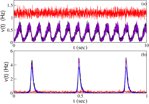
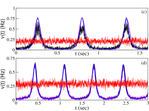
Figure 1: Population firing rates $\nu(t)$ versus time for $i_{0}=0.00055$: $K=10$ (a) and $K=210$ (b); $i_{0}=0.00033$ and $K=100$ (c) and $i_{0}=0.00027$ and $K=60$ (d). The black lines refer to network simulations with $N=80000$ neurons, the violet (red) lines to Langevin simulations with shot-noise (DA) with $N=20000$ (a-b) and $N=80000$ (c-d). The blue solid lines denote the results of the CMF approach (14,36). All data refer to $g_{0}=1$. Details on the integration of the Langevin equations are reported in Appendix B.

III Mean-field description

For a sufficiently sparse network with $K\ll N$, the spike trains emitted by $K$ pre-synaptic neurons can be assumed to be uncorrelated and Poissonian Brunel and Hakim (1999), therefore the mean-field dynamics of a QIF neuron can be represented in terms of the following Langevin equation:

$$\dot{V}(t)=V^{2}+I-gS(t)$$ (6)

where $S(t)$ is a Poissonian train of $\delta$-spikes with rate $R(t)=K\nu(t)$, and $\nu(t)$ is the population firing rate self-consistently estimated. Usually the Poissonian spike trains are approximated within the DA Capocelli and Ricciardi (1971); Tuckwell (1988) as $S(t)=R(t)+\sqrt{R(t)}\xi(t)$, where $\xi(t)$ is a normalized Gaussian white noise signal.

However, the DA can fail in reproducing the neural dynamics. Indeed, as shown in Fig. 1 for sparse networks with different sets of parameters by employing the DA in Eq. (6) one obtains an asynchronous dynamics (red curve), while the network evolution is characterized by GOs (black lines), that can be recovered only by explicitly taking into account the Poissonian spike trains in Eq. (6) (violet lines). As shown in panel (b), the DA is unable to reproduce simulation results even with quite large in-degree ($K=210$) for sufficiently small $i_{0}$. On the other hand, the Langevin mean-field data with shot-noise are in good agreement with the simulations in all considered cases indicating the validity of this approach.

In the mean-field framework the population dynamics is usually described in terms of the membrane potential probability density function (PDF) $P(V,t)$, whose time evolution for the QIF model is given (according to (6)) by the continuity equation

$${\partial_{t}P}(V,t)+\partial_{V}[(V^{2}+I)P(V,t)]=R(t)\Delta P(V,T)$$ (7)

with boundary condition $\lim_{V\to\infty}V^{2}P(V,t)=\nu(t)$ and where $\Delta P(V,T)=[P(V^{+},t)-P(V,t)]$ with $V^{+}=V+g$. The right-hand side term in (7) represents the time variation of $P(V,t)$ due to the arrival of the Poissonian trains of instantaneous inhibitory kicks of amplitude $g$ from $K$ pre-synaptic neurons. By assuming that $g$ is sufficiently small we can expand the latter term as

$$\Delta P(V,t)=\sum_{p=1}^{\infty}\frac{g^{p}}{p!}\partial_{V}^{p}P(V,t)\enskip;$$ (8)

and by limiting to the first two terms in this expansion we recover the DA corresponding to the following Fokker-Planck Equation (FPE) Haskell et al. (2001)

$${\partial_{t}P(V,t)}+{\partial_{V}}[(V^{2}+A(t))P(V,t)]=D(t){\partial^{2}_{V}P(V,t)}$$ (9)

where $A(t)=\sqrt{K}[i_{0}-g_{0}\nu(t)]$ is the effective input current and $D(t)=g_{0}^{2}\nu(t)/2$ represents the diffusion coefficient.

In the following we will consider also a generalized version of the FPE (GFPE) obtained by considering up to the third order term in the expansion (8), which gives the following evolution equation for the $P(V,t)$

$${\partial_{t}P(V,t)}+{\partial_{V}}[(V^{2}+A(t))P(V,t)]=D(t){\partial^{2}_{V}P(V,t)}+H(t){\partial^{3}_{V}P(V,t)}\quad,$$ (10)

where $H(t)=\frac{g_{0}^{3}\nu(t)}{3!\sqrt{K}}$ .

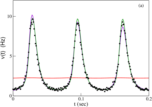
Figure 2: Population firing rates $\nu(t)$ versus time for $i_{0}=0.02$, $K=200$ (a) and $i_{0}=0.006$, $K=400$ (b). The black circles refer to network simulations with $N=80000$ (a) and $N=20000$ (b), the violet (red) solid lines to integration of the continuity equation (7) (FPE (9)). The green solid lines denote the results of the integration of the GFPE including third order terms (10). All data refer to $g_{0}=1$, the numerical integration of the partial differential equations has been performed by employing time splitting pseudo-spectral methods with a time step $\Delta t=10^{-4}$ ms and with 128–512 Fourier modes (for more details see Appendix C).

Comparisons among the network simulations (black circles) and the results obtained by integrating the partial differential equations (7) (violet line), (9) (red lines) and (10) (green lines) via time splitting pseudo-spectral methods (as explained in details in Appendix C) are shown in Fig. 2. These results show that DA can give incorrect predictions even at the level of population dynamics. Indeed, as shown in Fig. 2 (a) the network dynamics is oscillatory with $f_{G}\simeq 15$ Hz (black circles). This evolution is correctly captured by the continuity equation (7) (violet line). On the contrary, the FPE (9) (red line) converges to a stable fixed point corresponding to asynchronous dynamics. In this case, the inclusion of the third order term of the expansion (8) in the evolution equation for $P(V,t)$ (10) gives a stable solution (green solid line) capturing quite well the network dynamics. Unfortunately, this is not always the case due to the intrinsic instability of the third order expansion Marcinkiewicz (1939); Gardiner (1997), that e.g. does not guarantee that the sign of the PDF remains positive, as observable in the case reported in panel (b). In this latter situation, the DA is able to reproduce the oscillatory behaviour displayed by the network evolution, however the amplitudes of such oscillations are definitely better captured by the continuity equation (7) (violet line).

In summary, to correctly reproduce the collective dynamical regimes observable in the network it is necessary to consider the complete continuity equation (7), even if in some cases the third order expansion (10) could be sufficiently accurate. As a general remark the time splitting pseudo-spectral integration methods here employed suffer of numerical instabilities in particular for small $K$, that render the approach not particularly reliable. Therefore, as we will explain in the following we have developed an accurate and stable formalism encompassing synaptic shot-noise to identify the various possible regimes displayed by (7) and to characterize their linear and non-linear stability.

III.1 Derivation of the macroscopic evolution equations

As already mentioned, the dynamical evolution of the QIF model can be transformed in that of a phase oscillator, the $\theta$-neuron Ermentrout and Kopell (1986); Ermentrout (2008), by introducing the phase variable $\theta=2\arctan{V}$. However, this transformation renders quite difficult to distinguish asynchronous from partially synchronized states Kralemann et al. (2007); Dolmatova et al. (2017). A more suitable phase transformation, able to take into account correctly the phase synchronization phenomena, is the following

$$\psi=2\arctan\frac{V}{\sqrt{I}}\in[-\pi,\pi]\;,\qquad V=\sqrt{I}\tan\frac{\psi}{2}\in]-\infty,+\infty[\;,$$

where $I=i_{0}\sqrt{K}$. Indeed, for $I>0$ and in the absence of incoming pulses the phase $\psi$ is uniformly rotating with angular velocity $2\sqrt{I}$ at variance with the $\theta$-neuron where even for uncoupled oscillators the velocity depends on the phase.

The probability distribution function (PDF) $w(\psi)$ for the phase variables $\psi$ is related to the one of the membrane potentials $P(V,t)$ via the relation

$$w(\psi,t)=P(V,t)\frac{I+V^{2}}{2\sqrt{I}}$$

due to the probability conservation under (non-linear) transformations of stochastic variables. Therefore, the continuity equation (7) for $P(V,t)$ :

$$\frac{\partial P(V,t)}{\partial t}=-\frac{\partial}{\partial V}\Big{[}\big{(}I+V^{2}\big{)}P(V,t)\Big{]}+K\nu(t)\Big{[}P(V+g,t)-P(V,t)\Big{]}\;,$$ (11)

can be recast as follows for $w(\psi,t)$

$$\frac{\partial w(\psi,t)}{\partial t}=-\frac{\partial}{\partial\psi}\left[2\sqrt{I}w(\psi,t)\right]+K\nu(t)\left[\frac{I+V^{2}}{I+(V+g)^{2}}w(\psi_{+},t)-w(\psi,t)\right]\;,$$ (12)

where $\psi_{+}$ is the shifted phase:

$$V+g=\sqrt{I}\tan\frac{\psi_{+}}{2}\;,\qquad\tan\frac{\psi_{+}}{2}=\alpha+\tan\frac{\psi}{2}\;,\qquad\alpha\equiv\frac{g}{\sqrt{I}}=\frac{g_{0}}{\sqrt{i_{0}}K^{3/4}}\;.$$

By making all the terms in the right-end side of Eq. (12) explicit in terms of the variable $\psi$

$$\frac{I+V^{2}}{I+(V+g)^{2}}=\frac{1+\tan^{2}\frac{\psi}{2}}{1+\left(\alpha+\tan\frac{\psi}{2}\right)^{2}}=\frac{1}{1+\frac{\alpha^{2}}{2}+\alpha\sin\psi+\frac{\alpha^{2}}{2}\cos\psi}\;,$$

we can finally rewrite Eq. (12) as

$$\frac{\partial w(\psi,t)}{\partial t}=-\frac{\partial}{\partial\psi}\left[2\sqrt{I}w(\psi,t)\right]+K\nu(t)\left[\frac{w(\psi_{+},t)}{1+\frac{\alpha^{2}}{2}+\alpha\sin\psi+\frac{\alpha^{2}}{2}\cos\psi}-w(\psi,t)\right]\;.$$ (13)

In Fourier space the PDF $w(\psi,t)$ can be expressed as

$$w(\psi,t)=\frac{1}{2\pi}\sum\limits_{n=-\infty}^{+\infty}z_{n}e^{-in\psi},$$

with $z_{0}=1$ and $z_{-n}=z_{n}^{\ast}$, where the complex coefficients $z_{n}$ are the so-called Kuramoto–Daido order parameters $z_{n}$ Kuramoto (2012); Daido (1992). In terms of these coefficients the continuity equation (13) becomes

$$\dot{z}_{n}=i2n\sqrt{I}z_{n}+K\nu(t)\left[\sum_{m=-\infty}^{+\infty}I_{nm}z_{m}-z_{n}\right]\;,$$ (14)

where

$$I_{nm}\equiv\frac{1}{2\pi}\int\limits_{0}^{2\pi}\frac{e^{in\psi}\left(e^{-i\psi_{+}}\right)^{m}\mathrm{d}\psi}{1+\frac{\alpha^{2}}{2}+\alpha\sin\psi+\frac{\alpha^{2}}{2}\cos\psi}\;.$$ (15)

In order to calculate the integrals $I_{nm}$, we need to express explicitely the term $e^{-i\psi_{+}}=\cos\psi_{+}-i\sin\psi_{+}$ entering in Eq. (15). In particular, by noticing that

$$\cos\psi_{+}=\frac{1-\tan^{2}\frac{\psi_{+}}{2}}{1+\tan^{2}\frac{\psi_{+}}{2}}\;,\qquad\sin\psi_{+}=\frac{2\tan\frac{\psi_{+}}{2}}{1+\tan^{2}\frac{\psi_{+}}{2}}\;,$$

and therefore that

$$e^{-i\psi_{+}}=\cos\psi_{+}-i\sin\psi_{+}=\frac{1-i\tan\frac{\psi_{+}}{2}}{1+i\tan\frac{\psi_{+}}{2}}=-\frac{\tan\frac{\psi}{2}+\alpha+i}{\tan\frac{\psi}{2}+\alpha-i}\;.$$

Moreover by expressing $\zeta\equiv e^{i\psi}$ as follows

$$\zeta\equiv e^{i\psi}=-\frac{\tan\frac{\psi}{2}-i}{\tan\frac{\psi}{2}+i}\;,\quad\mbox{ and hence }\;\tan\frac{\psi}{2}=i\frac{1-\zeta}{1+\zeta}\;,$$

one finally finds

$$e^{-i\psi_{+}} =-\frac{\alpha+2i+\alpha\zeta}{\alpha+(\alpha-2i)\zeta}\;.$$ (16)

By employing the above expression the integral (15) can be rewritten as

$$I_{nm} =\int\limits_{0}^{2\pi}\frac{(2\pi)^{-1}e^{in\psi}\left[-\frac{\alpha+2i+\alpha e^{i\psi}}{\alpha+(\alpha-2i)e^{i\psi}}\right]^{m}\mathrm{d}\psi}{1+\frac{\alpha^{2}}{2}-\frac{i\alpha}{2}(e^{i\psi}-e^{-i\psi})+\frac{\alpha^{2}}{4}(e^{i\psi}+e^{-i\psi})}=\oint\limits_{|\zeta|=1}\frac{(i2\pi)^{-1}\zeta^{n-1}\left[-\frac{\alpha+2i+\alpha\zeta}{\alpha+(\alpha-2i)\zeta}\right]^{m}\mathrm{d}\zeta}{1+\frac{\alpha^{2}}{2}-\frac{i\alpha}{2}(\zeta-\frac{1}{\zeta})+\frac{\alpha^{2}}{4}(\zeta+\frac{1}{\zeta})}$$

$$=\frac{1}{2\pi i}\oint\limits_{|\zeta|=1}\frac{4(-\alpha)^{m}\zeta^{n}(\zeta+\frac{\alpha+2i}{\alpha})^{m-1}}{\alpha(\alpha-2i)^{m+1}(\zeta+\frac{\alpha}{\alpha-2i})^{m+1}}\mathrm{d}\zeta\;.$$ (17)

To evaluate the complex integral in (17) we employ the residue theorem and therefore we should identify the poles of the integrand. We can limit our consideration to $n\geq 1$ since $z_{0}=1$, and $z_{-n}=z_{n}^{\ast}$, for $m\leq 0$ the integrand has the following pole

$$\zeta_{2}=-\frac{\alpha+2i}{\alpha}\;,$$

which is always beyond the unit circle since $|\frac{\alpha+2i}{\alpha}|^{2}=1+4/\alpha^{2}>1$ and, therefore, does not contribute to the integral $I_{nm}$. However, for $m\geq 0$ the integrand displays another pole located at

$$\zeta_{1}=-\frac{\alpha}{\alpha-2i}\quad.$$

This pole is always within the integration contour $|\zeta|=1$ since $|\frac{\alpha}{\alpha-2i}|^{2}=\frac{\alpha^{2}}{\alpha^{2}+4}<1$ and therefore it contributes to the integral (17).

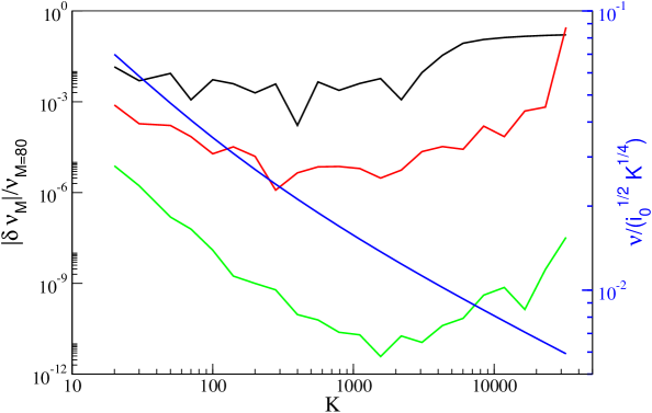
Figure 3: Relative error in the estimation of the firing rate $\nu$ for a stationary situation (asynchronous dynamics) computed with (14)–(36) plotted versus the in-degree $K$ for $M=10$ (black line), $20$ (red line), $40$ (green line). The reference firing rate was estimated by employing $M=80$ and it is shown in rescaled units as a blue line. Parameters: $(i_{0},g_{0})=(0.006,1)$.

We employ the residue theorem to evaluate the following integral:

$$\frac{1}{2\pi i}\oint\limits_{|\zeta|=1}\frac{\zeta^{n}(\zeta+\frac{\alpha+2i}{\alpha})^{m-1}}{(\zeta+\frac{\alpha}{\alpha-2i})^{m+1}}\mathrm{d}\zeta=\left\{\begin{array}[]{cr}\frac{1}{m!}\left.\frac{\mathrm{d}^{m}}{\mathrm{d}\zeta^{m}}\left(\zeta^{n}\left(\zeta-\zeta_{2}\right)^{m-1}\right)\right|_{\zeta=\zeta_{1}}\;,&m\geq 0\;;\\ 0\;,&m\leq-1\end{array}\right.$$ (20)

$$\qquad=\left\{\begin{array}[]{cc}\sum\limits_{j=0}^{\min(n,m)-1}\Big{(}{m-1\atop j}\Big{)}\Big{(}{n+m-1-j\atop m}\Big{)}\zeta_{1}^{n-1-j}\left(-\zeta_{2}\right)^{j}\;,&m\geq 1\;;\\[5.0pt] \frac{\zeta_{1}^{n}}{\zeta_{1}-\zeta_{2}}\;,&m=0\;;\\[5.0pt] 0\;,&m\leq-1\end{array}\right.$$ (24)

where $\min(n,m)$ returns the minimal of two values, the binomial coefficients are defined as $\left(n\atop m\right)=\frac{n!}{m!(n-m)!}$. In particular, for obtaining the result reported in the latter line we considered separately the cases for $1\leq n\leq m$ and for $n>m$. Hence,

$$I_{nm}(\alpha)=\left\{\begin{array}[]{cc}\sum\limits_{j=0}^{\min(n,m)-1}\frac{(\zeta_{1}-\zeta_{2})(n+m-1-j)!\cdot\zeta_{1}^{m+n-1-j}\left(-\zeta_{2}\right)^{j}}{m\cdot j!\cdot(m-1-j)!\cdot(n-1-j)!},&m\geq 1\,;\\[5.0pt] \zeta_{1}^{n}\;,&m=0\,;\\[5.0pt] 0\;,&m\leq-1\,.\end{array}\right.$$ (28)

After the substitution of the values of $\zeta_{1}$ and $\zeta_{2}$ in (28), the coefficients $I_{nm}(\alpha)$ take the form :

$$I_{nm}(\alpha)\equiv\frac{1}{2\pi}\int\limits_{0}^{2\pi}\frac{e^{in\psi}\left(e^{-i\psi_{+}}\right)^{m}\mathrm{d}\psi}{1+\frac{\alpha^{2}}{2}\alpha\sin\psi+\frac{\alpha^{2}}{2}\cos\psi}=\!\left\{\begin{array}[]{cr}\big{(}\frac{\alpha}{2i-\alpha}\big{)}^{n}\;,&m=0\,;\\[5.0pt] \sum\limits_{j=1}^{\min(n,m)}\frac{4(-1)^{j}(n+m-j)!\cdot\alpha^{m+n-2j}(4+\alpha^{2})^{j-1}}{m(j-1)!\cdot(m-j)!\cdot(n-j)!\cdot(2i-\alpha)^{m+n}},&m\geq 1\,.\end{array}\right.$$ (29)

In particular, for $n\geq 1$, one has $I_{nm}=0$ for $m<0$; therefore, the matrix $I_{nm}$ has non zero elements only for $n=1,2,3,...$ and $m=0,1,2,3,...$ :

$$\left(\frac{I_{nm}}{\zeta_{1}-\zeta_{2}}\right)=\left(\begin{array}[]{cccccllllll}\frac{\zeta_{1}}{\zeta_{1}-\zeta_{2}}&\zeta_{1}&\zeta_{1}^{2}&\zeta_{1}^{3}&\dots\\[5.0pt] \frac{\zeta_{1}^{2}}{\zeta_{1}-\zeta_{2}}&2\zeta_{1}^{2}&3\zeta_{1}^{3}-\zeta_{1}^{2}\zeta_{2}&4\zeta_{1}^{4}-2\zeta_{1}^{3}\zeta_{2}&\dots\\[5.0pt] \frac{\zeta_{1}^{3}}{\zeta_{1}-\zeta_{2}}&3\zeta_{1}^{3}&6\zeta_{1}^{4}-3\zeta_{1}^{3}\zeta_{2}&10\zeta_{1}^{5}-8\zeta_{1}^{4}\zeta_{2}+\zeta_{1}^{3}\zeta_{2}^{2}&\dots\\[5.0pt] \frac{\zeta_{1}^{4}}{\zeta_{1}-\zeta_{2}}&4\zeta_{1}^{4}&10\zeta_{1}^{5}-6\zeta_{1}^{4}\zeta_{2}&20\zeta_{1}^{6}-20\zeta_{1}^{5}\zeta_{2}+4\zeta_{1}^{4}\zeta_{2}^{2}&\dots\\[5.0pt] &\dots\end{array}\right).$$ (35)

In the continuity equation (12) appears the population firing rate $\nu(t)$ that should be evaluated self-consistently during the time evolution. The instantaneous firing rate is given by the flux at the firing threshold, therefore

$$\nu(t) =\lim_{V\to\infty}V^{2}P(V,t)=2\sqrt{I}\,w(\pi,t)=\frac{\sqrt{I}}{\pi}\mathrm{Re}\big{(}1-2z_{1}+2z_{2}-2z_{3}+2z_{4}-\dots\big{)}\;.$$ (36)

The dynamical system (14,36) has been numerically integrated with the exponential time differencing method Cox and Matthews (2002); Permyakova and Goldobin (2025) for time-dependent regimes and numerically solved (in the Maple analytical calculation package) for time-independent regimes, stability and weakly non-linear analyses by truncating the series $z_{n}$ at $n=M$ terms. Usually we fixed $M=100$ and, where necessary, $M$ was increased in order to keep the relative simulation error below $10^{-12}$ map (see Fig. 3).

III.2 Diffusion and third order approximations

Consider the continuity equation (10), which yields the DA with $H(t)$ set to zero and the D3A for $H(t)=g_{0}^{3}\nu(t)/(3!\sqrt{K})$, but recast it as

$${\partial_{t}P(V,t)}+{\partial_{V}}[(V^{2}+I)P(V,t)]=K\nu(t)\left[g\partial_{V}P(V,t)+\frac{g^{2}}{2}\partial^{2}_{V}P(V,t)+\frac{g^{3}}{3!}\partial^{3}_{V}P(V,t)\right]\quad.$$ (37)

For the probability density $w(\psi,t)$ of the phase variable $\psi=2\arctan(V/\sqrt{I})$, continuity equation (37) yields a modified version of (12) :

$$\frac{\partial w(\psi,t)}{\partial t}=-\frac{\partial}{\partial\psi}\left[2\sqrt{I}w(\psi,t)\right]+K\nu(t)\left[\frac{g}{\sqrt{I}}\mathcal{Q}w(\psi,t)+\frac{g^{2}}{2I}\mathcal{Q}^{2}w(\psi,t)+\frac{g^{3}}{3!I^{3/2}}\mathcal{Q}^{3}w(\psi,t)\right]\quad,$$ (38)

where the operator

$$\mathcal{Q}(\dots)\equiv\frac{\partial}{\partial\psi}\Big{[}(1+\cos\psi)(\dots)\Big{]}\,.$$

Hence, for the Kuramoto–Daido order parameters $z_{n}$, one finds a modified version of equation system (14):

$$\dot{z}_{n}=i2n\sqrt{I}z_{n}+K\nu(t)\sum_{m=0}^{+\infty}I_{nm}^{[\mathrm{tr}]}z_{m}\;,\quad n=1,2,3,\dots,$$ (39)

where $z_{0}=1$; for DA, the “truncated” matrix

$$I_{nm}^{[\mathrm{tr}]}=I_{nm}^{[\mathrm{DA}]}\equiv\alpha Q_{nm}+\frac{\alpha^{2}}{2}(\mathcal{Q}^{2})_{nm}$$

and, for D3A,

$$I_{nm}^{[\mathrm{tr}]}=I_{nm}^{[\mathrm{D3A}]}\equiv\alpha Q_{nm}+\frac{\alpha^{2}}{2}(\mathcal{Q}^{2})_{nm}+\frac{\alpha^{3}}{3!}(\mathcal{Q}^{3})_{nm}.$$

In Fourier space, operator $\mathcal{Q}$ has the following matrix form:

$$Q_{nm}=\left(\begin{array}[]{ccccccc}0&0&0&0&0&\dots\\ -\frac{i}{2}&-i&-\frac{i}{2}&0&0&\dots\\ 0&-i&-2i&-i&0&\dots\\ 0&0&-\frac{3i}{2}&-3i&-\frac{3i}{2}&\dots\\ &\dots&&\end{array}\right)\,,$$

where the numbers of rows and columns run from $n=0$ and $m=0$, respectively; and matrices $\mathcal{Q}^{2}$, $\mathcal{Q}^{3}$ can be easily calculated via conventional matrix multiplication. By substituting the matrix coefficients, one can recast Eq. (39) as follows:

$$\dot{z}_{n} \textstyle=i2n\sqrt{I}z_{n}+K\nu(t)\Big{\{}\frac{n\alpha}{i}\left(z_{n}+\frac{z_{n\pm 1}}{2}\right)-\frac{n\alpha^{2}}{2}\left[\frac{3n}{2}z_{n}+\left(n\pm\frac{1}{2}\right)z_{n\pm 1}+\frac{n\pm 1}{4}z_{n\pm 2}\right]$$

$$\textstyle+\frac{in\alpha^{3}}{6}\left[\frac{5n^{2}+1}{2}z_{n}+\frac{15n(n\pm 1)+6}{8}z_{n\pm 1}+\frac{3(n\pm 1)^{2}}{4}z_{n\pm 2}+\frac{(n\pm 1)(n\pm 2)}{8}z_{n\pm 3}\right]\Big{\}}\quad,$$ (40)

where the terms with $\pm$ are not alternative, but they should be considered as both present in the sum of the terms on the right-hand side and the diffusion approximation can be obtained by omitting the $\alpha^{3}$-term. By employing the system of equations (39) (or (40)) we can deal with the DA and the D3A in technically the same way as done for the CMF model (14), once replaced the matrix $\left(I_{nm}(\alpha)-\delta_{nm}\right)$ with $I_{nm}^{[\mathrm{tr}]}(\alpha)$.

III.3 Linear stability of the asynchronous regime

In order to analyzie the stability of the asynchronous dynamics and the emergence of global oscillations in the macroscopic evolution, we rewrite the system (14,36) as follows :

$$\frac{\mathrm{d}z_{n}}{\mathrm{d}t} =F_{n}(z_{1},z_{2},z_{3},\dots)$$

$$=\sqrt{i_{0}}K^{\frac{1}{4}}\Bigg{(}i2nz_{n}+K\widetilde{\nu}\Big{[}I_{n0}(\alpha)+\sum_{m=1}^{+\infty}I_{nm}(\alpha)\,z_{m}-z_{n}\Big{]}\Bigg{)}\,,$$ (41)

with

$$\widetilde{\nu}=\frac{\nu}{\sqrt{I}}=\frac{1}{\pi}\mathrm{Re}(1-2z_{1}+2z_{2}-2z_{3}+2z_{4}-\dots)\,.$$ (42)

As a first aspect we notice that the dynamical evolution of the system (41)–(42) is controlled by two dimensionless parameters, namely

$$K\quad\mbox{ and }\quad\alpha=\frac{g_{0}}{\sqrt{i_{0}}K^{3/4}}\,,$$

while the time can be rescaled by the factor $\sqrt{I}=\sqrt{i_{0}}K^{1/4}$. Therefore a bifurcation diagram in the plane $(K,i_{0}/g_{0}^{2})$ is sufficient to capture all possible dynamical regimes observable for the system (41)–(42).

In order to analyze the stability of the stationary regimes in this plane, we should linearize the system (41)–(42) around a fixed point solution $\{{z}_{n}^{(0)}\}$. In particular, since $F_{n}$ depend on $\widetilde{\nu}$, which is non analytic function of $z_{m}$, the linearization of (41) should be performed by considering as independent variables the real and imaginary parts of the Kuramoto–Daido order parameters : namely, $z_{n}^{\mathrm{re}}=\mathrm{Re}(z_{n})$ and $z_{n}^{\mathrm{im}}=\mathrm{Im}(z_{n})$ (here and hereafter, superscripts “$\mathrm{re}$” and “$\mathrm{im}$” denote the real and imaginary parts).

Therefore the linearization of (41) can be written as

$${\delta\dot{x}}_{2n-1} = \frac{\partial F_{n}^{\mathrm{re}}}{\partial z_{m}^{\mathrm{re}}}{\delta x}_{2n-1}+\frac{\partial F_{n}^{\mathrm{re}}}{\partial z_{m}^{\mathrm{im}}}{\delta x}_{2n}$$ (43)

$${\delta\dot{x}}_{2n} = \frac{\partial F_{n}^{\mathrm{im}}}{\partial z_{m}^{\mathrm{re}}}{\delta x}_{2n-1}+\frac{\partial F_{n}^{\mathrm{im}}}{\partial z_{m}^{\mathrm{im}}}{\delta x}_{2n}$$ (44)

where ${\delta x}_{2n-1}$ and ${\delta x}_{2n}$ are the infinitesimal perturbations of the real and imaginary parts of $z_{n}$, respectively. Moreover, the other terms entering in (43)–(44) can be explicitly written as

$$\frac{\partial F_{n}^{\mathrm{re}}}{\partial z_{m}^{\mathrm{re}}} =\sqrt{i_{0}}K^{\frac{1}{4}}\bigg{(}K\widetilde{\nu}\big{(}I_{nm}^{\mathrm{re}}-\delta_{nm}\big{)}+\frac{4n(-1)^{m}}{\pi\widetilde{\nu}}\big{[}{z}^{(0)}_{n}\big{]}^{\mathrm{im}}\bigg{)}\,,$$ (45a)

$$\frac{\partial F_{n}^{\mathrm{im}}}{\partial z_{m}^{\mathrm{re}}} =\sqrt{i_{0}}K^{\frac{1}{4}}\bigg{(}2n\delta_{nm}+K\widetilde{\nu}I_{nm}^{\mathrm{im}}-\frac{4n(-1)^{m}}{\pi\widetilde{\nu}}\big{[}{z}^{(0)}_{n}\big{]}^{\mathrm{re}}\bigg{)}\,,$$ (45b)

$$\frac{\partial F_{n}^{\mathrm{re}}}{\partial z_{m}^{\mathrm{im}}} =\sqrt{i_{0}}K^{\frac{1}{4}}\left(-2n\delta_{nm}-K\widetilde{\nu}I_{nm}^{\mathrm{im}}\right)\;,$$ (45c)

$$\frac{\partial F_{n}^{\mathrm{im}}}{\partial z_{m}^{\mathrm{im}}} =\sqrt{i_{0}}K^{\frac{5}{4}}\widetilde{\nu}\big{(}I_{nm}^{\mathrm{re}}-\delta_{nm}\big{)}\;.$$ (45d)

The linear stability analysis of time-independent solutions ${\bf z}^{(0)}=\{{z}_{n}^{(0)}\}$ of system (41)–(42) can be performed by solving the eigenvalue problems associated to Eqs. (43)–(44). In particular, by truncating the system (41)–(42) to the $M$-th Kuramoto–Daido order parameter the eigenvalue problem can be solved for a $(2M\times 2M)$ matrix with real-valued elements given by (45) to find the associated complex eigenvalue spectrum $\{\lambda_{j}\}\quad j=1,\dots,2M$. The stationary solution is stable whenever $\mathrm{Re}\enskip\lambda_{j}<0\quad\forall j$.

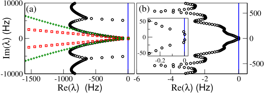
Figure 4: Spectrum of the eigenvalues $\{\lambda_{i}\}$ for a stationary solution of the system (14,36) for $(i_{0}/g_{0}^{2},K)=(0.02,400)$ (a), and $(0.00055,10)$ (b). An enlargement is reported in the inset in (b). Black circles refer to the CMF, the red squares to the DA and the green pluses to the D3A.

Let us compare the spectra obtained within the CMF, the DA and the D3A to better understand the origin of the instabilities leading to oscillatory dynamics in the presence of microscopic shot-noise. As a first remark, we observe that the DA and D3A spectra are characterized besides the most unstable modes, which can give rise to the oscillatory instability, by modes that are strongly damped as shown in Fig. 4 (a). The case shown in Fig. 4 (a) refers to a situation where the dynamics is well reproduced already within the DA (red circles), in this case the DA and D3A (green pluses) eigenvalues corresponding to small ${\rm Im}\enskip\lambda_{j}$ in proximity of the Hopf instability approximate quite well the CMF spectrum (black circles). However, while the CMF eigenvalues appear to saturate at some finite ${\rm Re}\enskip\lambda$ value, the DA and D3A ones do not. We also notice that the D3A captures extremely well the central part of the CMF spectrum, while the DA deviates quite soon from it. Despite these differences in this case the collective dynamics of the system is essentially controlled by the two most unstable modes, typical of a Hopf bifurcation, that practically coincide within the three approaches.

In Fig. 4 (b) we report the CMF spectrum for a situation where the oscillatory regime is definitely due to the finitness of the synaptic stimulations and not captured at all by the DA and D3A. In this case, we observe that a large part of the eigenmodes are now practically undamped, compare the scales over which ${\rm Re}\enskip\lambda_{j}$ varies in Fig. 4 (a) and (b). Therefore, we expect that the collective dynamics is no longer dominated by only the 2 most unstable modes as usually observable in the DA, but that also the marginally stable or slightly unstable modes will contribute in the coherent dynamics, see the inset of panel (b).

In summary, the shot-noise promotes the emergence of weakly damped eigenmodes that have a relevant role in the instability of the asynchronous regime at sufficiently small $i_{0}/g_{0}^{2}$ and in-degrees and that are neglected in the DA.

III.4 Weakly Non-Linear Analysis

As for the linear stability, also for the weakly non-linear analysis required to characterize the nature of the observed Hopf bifurcations, one must handle $z_{n}^{\mathrm{re}}$ and $z_{n}^{\mathrm{im}}$ as independent real-valued variables. In particular, it is important to stress that the dynamical system (41,42) is quadratic with respect to the variables $z_{n}^{\mathrm{re}}$ and $z_{n}^{\mathrm{im}}$. The absence of cubic terms makes the calculation of the coefficients of the amplitude equations quite simple as we will see in the following.

Let us now analyse the Hopf instability of the stationary solution $\mathbf{z}^{(0)}=\{z_{1}^{(0)},z_{2}^{(0)},z_{3}^{(0)},\dots\}$ in proximity to the critical value $K_{\mathrm{cr}}$, where the in-degree $K$ acts as the control parameter and $i_{0}$ and $g_{0}$ are maintained constant. In order to perform this analysis we have considered finite perturbations $\mathbf{x}=\{x_{1},x_{2},x_{3},x_{4},\dots\}$ of the stationary solution, where $x_{m}$ are real-valued variables defined as follows: $z_{n}^{\mathrm{re}}\equiv(z_{n}^{(0)})^{\mathrm{re}}+x_{2n-1}$, $z_{n}^{\mathrm{im}}\equiv(z_{n}^{(0)})^{\mathrm{im}}+x_{2n}$. To obtain an exact evolution equation for the perturbations, we have substituted $z_{n}=z_{n}^{(0)}+x_{2n-1}+ix_{2n}$ into the system (41,42). Furthermore, by remembering that $\mathbf{z}^{(0)}$ solves the right-hand side of the system (41,42), and rearranging the terms, one can arrive to the following system of differential equations ruling the dynamics of $\mathbf{x}$:

$$\frac{\mathrm{d}x_{n}}{\mathrm{d}t}=F_{nm}x_{m}+\widetilde{F}_{nml}x_{m}x_{l}\,,$$ (46)

where we imply the Einstein summation rule over repeated indices, odd-indexed(even-indexed) $x_{n}$ are the perturbations of the real (imaginary) part of $z_{m}$. All the linear in $\mathbf{x}$ terms appearing in (46) correspond to those obtained within the linear stability analysis, therefore, the coefficients (45) calculated at $\mathbf{z}^{(0)}$ correspond to the coefficients $F_{nm}$ as follows:

$$F_{2n-1\;2m-1}=\left.\frac{\partial F_{n}^{\mathrm{re}}}{\partial z_{m}^{\mathrm{re}}}\right|_{\mathbf{z}^{(0)}},\quad \quad F_{2n\;2m-1}=\left.\frac{\partial F_{n}^{\mathrm{im}}}{\partial z_{m}^{\mathrm{re}}}\right|_{\mathbf{z}^{(0)}},$$

$$F_{2n-1\;2m}=\left.\frac{\partial F_{n}^{\mathrm{re}}}{\partial z_{m}^{\mathrm{im}}}\right|_{\mathbf{z}^{(0)}},\quad \quad F_{2n\;2m}=\left.\frac{\partial F_{n}^{\mathrm{im}}}{\partial z_{m}^{\mathrm{im}}}\right|_{\mathbf{z}^{(0)}}.$$

Further, we need to collect all the terms quadratic in $\mathbf{x}$ which can only originate from the following term in Eq. (41):

$$K\left(\widetilde{\nu}-\pi^{-1}\right)\sum_{m=1}^{+\infty}(I_{nm}-\delta_{nm})z_{m}=\sum_{m,m^{\prime}}\frac{2K(-1)^{m^{\prime}}}{\pi}(I_{nm}-\delta_{nm})z_{m}z_{m^{\prime}}^{\mathrm{re}}\,;$$

substituting $z_{n}=z_{n}^{(0)}+x_{2n-1}+ix_{2n}$ into the latter expression and taking the real and imaginary parts, one can collect all the quadratic $x_{m}x_{l}$-terms:

$$\widetilde{F}_{2n-1\,ml}x_{m}x_{l} =\sum_{m,m^{\prime}}\frac{2\sqrt{i_{0}}K^{\frac{5}{4}}(-1)^{m^{\prime}}}{\pi}\big{[}\left(I_{nm}^{\mathrm{re}}-\delta_{nm}\right)x_{2m-1}-I_{nm}^{\mathrm{im}}x_{2m}\big{]}x_{2m^{\prime}-1}\,,$$

$$\widetilde{F}_{2n\,ml}x_{m}x_{l} =\sum_{m,m^{\prime}}\frac{2\sqrt{i_{0}}K^{\frac{5}{4}}(-1)^{m^{\prime}}}{\pi}\big{[}\left(I_{nm}^{\mathrm{re}}-\delta_{nm}\right)x_{2m}+I_{nm}^{\mathrm{im}}x_{2m-1}\big{]}x_{2m^{\prime}-1}\,.$$

Since the original equation system (41,42) contained only quadratic in $\mathbf{z}$ terms, we will also only have linear and quadratic in $\mathbf{x}$ terms.

For the weakly non-linear analysis of a bifurcation, we have to consider dynamical system (46) in a small vicinity of the bifurcation point $K_{\mathrm{cr}}(i_{0},g_{0})$, where

$$\frac{\mathrm{d}x_{n}}{\mathrm{d}t}=F_{nm}(K_{\mathrm{cr}})\,x_{m}+\widetilde{F}_{nml}(K_{\mathrm{cr}})\,x_{m}x_{l}+(K-K_{\mathrm{cr}})\left(\frac{\partial F_{nm}}{\partial K}\right)_{i_{0},g_{0}}x_{m}\,,$$ (47)

and $\left(\frac{\partial\dots}{\partial K}\right)_{i_{0},g_{0}}$ indicates the derivative with respect to $K$ for fixed $i_{0}$, $g_{0}$. Below we will omit the argument $K_{\mathrm{cr}}$ for coefficients $F_{nm}$ and $\widetilde{F}_{nml}$ for brevity.

At a Hopf instability, the most unstable modes are associated to two purely imaginary and complex conjugate eigenvalues. Therefore the linear stability matrix $(F_{nm})$ has a pair of eigenvalues $\pm i\Omega\equiv\pm i2\pi f^{H}$ with eigenvector $\mathbf{Y}$ and $\mathbf{Y}^{\ast}$, namely:

$$i\Omega Y_{n}=F_{nm}Y_{m}\,,\qquad-i\Omega Y_{n}^{\ast}=F_{nm}Y_{m}^{\ast}\,,$$ (48)

and the Hermitian conjugate problem possesses eigenvalues $\mp i\Omega$ with eigenvectors $\mathbf{Y}^{+}$ and $(\mathbf{Y}^{+})^{\ast}$ :

$$-i\Omega Y_{n}^{+}=F_{mn}Y_{m}^{+}\,,\qquad i\Omega(Y_{n}^{+})^{\ast}=F_{mn}(Y_{m}^{+})^{\ast}\,.$$ (49)

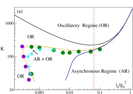
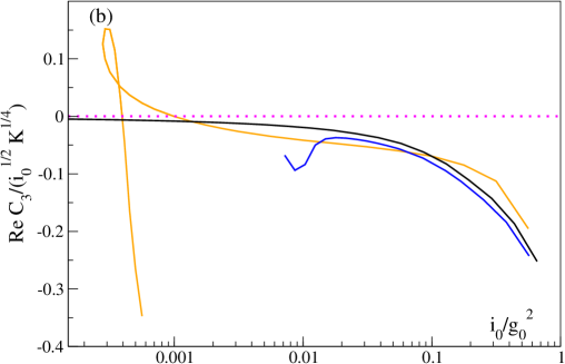
Figure 5: (a) Phase diagram for the QIF network in the plane $(i_{0}/g_{0}^{2},K)$: the black (blue) solid line is the super-critical HB line obtained within the DA (D3A); the orange solid (dashed) line is the super- (sub-) critical HB line given by the CMF; the symbols refer to numerical estimations of the HBs and SNBs. The green (violet) circles denote HBs obtained by performing quasi-adiabatic simulations by varying $K$ ($i_{0}$) for constant $i_{0}$ ($K$) values; the cyan stars indicate SNBs. The dimension of symbols takes in account for the error bar in the transition point evaluation. The vertical red dotted line is the critical value defined in Di Volo et al. (2022) within the DA for the emergence of fluctuation-driven balanced asynchronous dynamics (for more details see the text). (b) The coefficient $\mathrm{Re}\,C_{3}$ in rescaled units at the critical points $K=K_{cr}$ versus $i_{0}/g_{0}^{2}$: CM orange solid line), DA (black line) and D3A (blue line). In all the simulation $g_{0}=1$.

To find the amplitude equation we employ the standard multiple scale method Kuramoto (2012); Nayfeh (2024) with formal small parameter $\varepsilon$ ; $\frac{\mathrm{d}}{\mathrm{d}t}=\frac{\partial}{\partial t_{0}}+\varepsilon\frac{\partial}{\partial t_{1}}+\varepsilon^{2}\frac{\partial}{\partial t_{2}}+\dots$, $x_{n}=\varepsilon x_{n}^{(1)}+\varepsilon^{2}x_{n}^{(2)}+\varepsilon^{3}x_{n}^{(3)}+\dots$, where $t_{0}$ is the time scale related to the period of the emergent oscillation and $t_{1}$, $t_{2}$ are the “slow” time scales— associated to the modulation of the oscillation amplitude. In proximity of a Hopf bifurcation one expects the following scaling $|\mathbf{x}|\sim(K-K_{\mathrm{cr}})^{1/2}$ for the oscillation amplitude, thus suggesting to expand the control parameter as $K=K_{\mathrm{cr}}+\varepsilon^{2}K_{2}$, where $\varepsilon^{2}K_{2}$ is the deviation from the bifurcation point.

By substituting these expansions in Eq. (47) we obtain at the first order in $\varepsilon$ the following expression

$$x_{n}^{(1)}=A(t_{1},t_{2},\dots)Y_{n}e^{i\Omega t_{0}}+c.c.\,.$$

And at the order $\varepsilon^{2}$:

$$\frac{\partial x_{n}^{(2)}}{\partial t_{0}}+\frac{\partial A}{\partial t_{1}}Y_{n}e^{i\Omega t_{0}}+c.c.=F_{nm}x_{m}^{(2)}+\widetilde{F}_{nml}\big{[}A^{2}Y_{m}Y_{l}e^{i2\Omega t_{0}}+c.c.+|A|^{2}(Y_{m}Y_{l}^{\ast}+Y_{m}^{\ast}Y_{l})\big{]}\,.$$

One finds $\partial A/\partial t_{1}=0$ and

$$x_{n}^{(2)}=A^{2}\chi_{n}e^{i2\Omega t_{0}}+c.c.+|A|^{2}\phi_{n}\,,$$

where $\phi_{n}$ is the solution of the linear equation system

$$F_{nm}\phi_{m}=-\widetilde{F}_{nml}(Y_{m}Y_{l}^{\ast}+Y_{m}^{\ast}Y_{l})\,,$$

and $\chi_{n}$ is the solution of

$$(F_{nm}-i2\Omega\delta_{nm})\chi_{m}=-\widetilde{F}_{nml}Y_{m}Y_{l}\,.$$

At the order $\varepsilon^{3}$, we find the solvability condition,

$$\frac{\partial A}{\partial t_{2}}(Y_{n^{\prime}}^{+})^{\ast}Y_{n^{\prime}}=K_{2}A(Y_{n}^{+})^{\ast}\left(\frac{\partial F_{nm}}{\partial K}\right)_{i_{0},g_{0}}\!Y_{m}$$

$$+A|A|^{2}(Y_{n}^{+})^{\ast}\widetilde{F}_{nml}\left(Y_{m}^{\ast}\chi_{l}+\chi_{m}Y_{l}^{\ast}+Y_{m}\phi_{l}+\phi_{m}Y_{l}\right)\,.$$

The latter is the so-called amplitude equation and it can be recast in the standard form

$$\frac{\partial A}{\partial t}=(K-K_{\mathrm{cr}})\frac{\mathrm{d}\lambda}{\mathrm{d}K}A+C_{3}A|A|^{2}\,,$$ (50)

where $A$ is the complex amplitude of oscillations, $x_{n}=AY_{n}e^{i\Omega t}+c.c.+\mathcal{O}(A^{2})$; $\lambda$ is the exponential growth rate of the leading mode. The expression of the coefficient $C_{3}$ being the following:

$$C_{3}=\frac{(Y_{n}^{+})^{\ast}\widetilde{F}_{nml}\left(Y_{m}^{\ast}\chi_{l}+\chi_{m}Y_{l}^{\ast}+Y_{m}\phi_{l}+\phi_{m}Y_{l}\right)}{(Y_{n^{\prime}}^{+})^{\ast}Y_{n^{\prime}}}\;.$$ (51)

The sign of the real part of $C_{3}$ identifies the Hopf bifurcation as sub-critical (super-critical) for $\mathrm{Re}\enskip C_{3}>0$ ($\mathrm{Re}\enskip C_{3}<0$).

The Hopf bifurcation lines obtained in the plane $(i_{0}/g_{0}^{2},K)$ with this approach are reported for CMF (orange line), DA (black line) and D3A (blue line) in Fig. 5 (a). For the DA and D3A the Hopf lines are always super-critical, this is not the case for the CMF, where they can be either super-critical (solid orange line) or sub-critical (dashed orange line). The sub- or super-critical nature of the Hopf bifurcation is decided on the basis of the sign of $\mathrm{Re}\enskip C_{3}$ displayed in Fig. 5 (b) as a function of $i_{0}/g_{0}^{2}$ at the critical points $K=K_{cr}$.

A peculiarity of the CMF results is that the HB line is re-entrant, thus in a certain range of $i_{0}/g_{0}^{2}$ we have an asynchronous regime only within a finite interval of in-degrees and GOs at sufficiently small and large $K$. As explained in the following these two oscillatory regimes are due to different mechanisms.

Furthermore, there is a dramatic difference among the CMF and D3A approaches and the DA at small $i_{0}$ (large $g_{0})$: within the DA GOs are observable only above a critical $K$ diverging to infinity for $i_{0}/g_{0}^{2}\to 0$, while for the CMF (D3A) analysis GOs are present at any $K$ value for $i_{0}/g_{0}^{2}<0.00029$ ($i_{0}/g_{0}^{2}<0.007$).

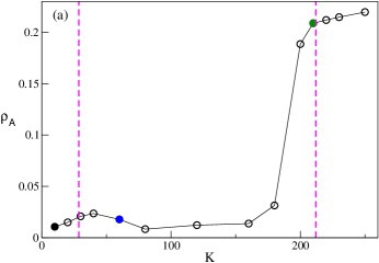
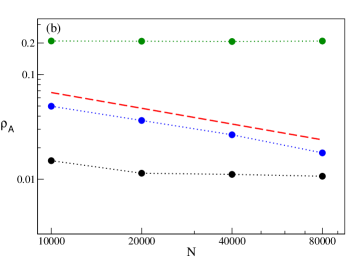
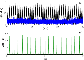
Figure 6: Average order parameter $\rho_{A}$ versus $K$ (a) and versus the system size $N$ (b) for $K=10$ (black circles), $K=60$ (blue circles) and $K=210$ (green circles). In (a) the vertical magenta lines denote the HBs obtained within the CMF approach. In (b) the dotted lines are a guide for the eyes, while the red dashed line denotes a power-law decay $\propto N^{-1/2}$. The values of $\rho_{A}$ have been averaged over 5-20 network realizations for a time interval $t_{E}=20-30$ s following a transient of $t_{T}=20-30$ s. (c-d) Firing rates $\nu(t)$ versus time $t$ for $K=10$ (black line) and $K=60$ (blue line) in (c) and $K=210$ (green line) in (d). The data in (a) refer to quasi-adiabatic simulations for fixed $i_{0}$ obtained by increasing (decreasing) $K$ in steps $\Delta K=10-20$. All data refer to $i_{0}=0.00055$ and $g_{0}=1$, the simulations in (a) and (c-d) concern networks of size $N=80000$.

IV Network Simulations

In order to verify the CMF predictions we have performed extremely accurate numerical simulations of QIF networks, according to (1), by employing an event-driven integration scheme (see Appendix A for more information), which allowed us to follow the network dynamics for long times, up to $60-100$ sec, for systems of size $N=10000-80000$. The CMF (14,36) is able to reproduce reasonably well network simulations (black curves) as shown by the data reported in Fig. 1 (b-d) for various values of $K$ and $i_{0}$. Furthermore, also the agreement between the Langevin results with shot-noise (violet curve) and the CMF (blue curve) is definitely good for $K>20$, as shown in Fig. 1 (b-d). These comparisons confirm the validity of the considered CMF approach.

Let us now compare the bifurcation diagrams obtained within the CMF approach and via extensive numerical simulations. In particular, to characterize the macroscopic evolution of the network we measured the indicator $\rho_{A}$ (4) averaged over several different network realizations. As we will show in the following a finite-size analysis of this order parameter has allowed us to identify numerically the Hopf (HBs) and the Saddle-Node Bifurcations (SNBs). This analysis is essentially based on the fact that a coherent macroscopic activity is characterized by a value of $\rho_{A}$ remaining finite in the thermodynamic limit (irrespective of its value), while asynchronous dynamics is associated to a vanishing $\rho_{A}$, indeed from the central limit theorem one expects that $\rho_{A}\propto N^{-1/2}$ for $N\to\infty$ Ullner and Politi (2016); di Volo and Torcini (2018).

The results of this analysis are reported in Fig. 5(a) green (magenta) circles refer to HBs identified via quasi-adiabatic simulations by varying $K$ ($i_{0}$) for constant $i_{0}$ ($K$) values; while the cyan stars indicate SNBs. Numerical simulations are in good agreement with the CMF results and allowed us also the identification of a coexistence region for asynchronous and oscillatory collective dynamics.

In large part of the phase diagram (namely, for $i_{0}/g_{0}^{2}<0.1$), both in the AR and OR we observe an irregular firing activity of the neurons associated to population averaged coefficient of variations ${CV}\simeq 0.8-1.0$, as expected in sparse balanced networks. This is consistent with the analysis reported in Di Volo et al. (2022), where within the DA a critical value $i_{0}/g_{0}^{2}=0.0637\dots$ separating fluctuation-driven from mean-driven balanced asynchronous dynamics Lerchner et al. (2006) has been identified in the thermodynamic limit. This value, shown in Fig. 5 (a) as a red dotted vertical line, can be considered as a lower limit, below which the spiking activity is definitely irregular.

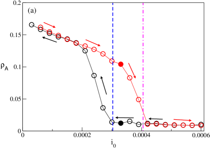
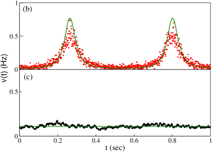
Figure 7: (a) Average order parameter $\rho_{A}$ versus $i_{0}$ for $K=100$. The blue dashed line in (a) denotes the sub-critical HB given by the CMF and the magenta dot-dashed line: numerically estimated SNB. In (b-c) the population firing rates $\nu(t)$ versus time are reported for the states indicated by the corresponding colored filled circles, the results for the CMF are also shown as green solid lines. The data in (a) refer to quasi-adiabatic simulations for fixed in-degree obtained by increasing (decreasing) $i_{0}$ in steps $\Delta i_{0}=0.00003$. The values of $\rho_{A}$ in (a) have been averaged over $5$ network realizations for $t_{E}=30$ s following a transient of $t_{T}=20$ s. For all data $N=80000$ and $g_{0}=1$.

IV.1 Finite size characterization of the observed transitions

Let us now explain in details for two characteristic cases how we proceeded to estimate numerically the transitions. In order to compare simulations done for a finite network to the CMF results obtained in the limit $N\to\infty$ it is necessary to average over different network realizations, to reduce finite size effects. The HBs and SNBs reported in Fig. 5 (a) have been obtained by performing finite size analysis of the order parameter $\rho_{A}$ obtained during quasi-adiabatic simulations of the QIF network by varying $K$ ($i_{0}$) for constant $i_{0}$ ($K$). In particular, the average value of the order parameter $\rho_{A}$ for each system size $N$ has been obtained by averaging over a time $t_{E}=20-30$ s after discarding a transient of $t_{T}=20-30$ s and over 5 to 20 different network realizations. Therefore, $\rho_{A}$ is obtained as a double average over time and over different random realizations of the connections among the neurons by maintaining $K$ constant, the latter amounts to average over realizations of the quenched disorder present in the network. According to the central limit theorem and analogously to what done in di Volo and Torcini (2018), we have classified the dynamical regimes by estimating the parameter $\rho_{A}$ for increasing system sizes $N$: if the indicator $\rho_{A}$ decreases as $1/\sqrt{N}$ (saturates to some constant value) then the dynamics is identified as asynchronous (oscillatory). The actual value of $\rho_{A}$ is just related to the level of synchronization in the neuronal population not to the specific macroscopic regime (asynchronous or GOS) displayed by the network.

Furthermore, as shown in Fig. 6 (a) for sufficiently small $i_{0}/g_{0}^{2}$ values, GOs are observable at small ($K\leq 30$) and large ($K\geq 200$) in-degrees, while the AR is present only at intermediate in-degrees ($K\in[40,180]$). The dynamics in these three intervals is visualized by reporting in Fig. 6 (c-d) the firing rates $\nu(t)$ at $K=10$ (black line), $K=60$ (blue line) (c) and $K=210$ (green line) (d).

In particular, we have estimated, for these three different values of the in-degree $K=10,60$, and 210, the scaling of $\rho_{A}$ for system sizes $N=10000$, 20000, 40000, and 80000. From Fig. 6 (a) we observe that for $K=10$ and $K=210$ (black and green symbols, respectively) $\rho_{A}$ saturates to some constant value and therefore we expect oscillatory dynamics as confirmed by the evolution of the population firing rate $\nu(t)$ reported in Fig. 6 (c-d). The value to which the indicator converges is irrelevant for the observation of GOs, it only indicates a different level of synchronization among the neurons. Indeed the neurons are much more synchronized for $K=210$ as shown in Fig. 6 (d) (green line), as compared to the case $K=10$ reported in Fig. 6 (c) (black line). For $K=60$ we observe that $\rho_{A}$ decreases as $1/\sqrt{N}$ as shown in Fig. 6 (b)(blue symbols) and as expected the population firing rate displays irregular fluctuations around a constant value, see Fig. 6 (c)(blue line), therefore the dynamics can be safely identified as asynchronous in this case. In this case we do not observe any hysteretic effect, consistently with what predicted by the CMF theory.

A hysteretic transition from AR to OR is instead obtained by varying quasi-adiabatically $i_{0}$ as displayed in Fig. 7 (a) for $K=100$ and $g_{0}=1$, the coexistence region can be clearly identified between the sub-critical HB (blue dashed line) and the SNB of limit cycles (magenta dot-dashed line). Two coexisting solutions are reported in Fig. 7 (b-c) confirming the good agreement between CMF (green lines) and the network simulations (red and black circles).

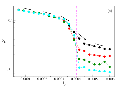
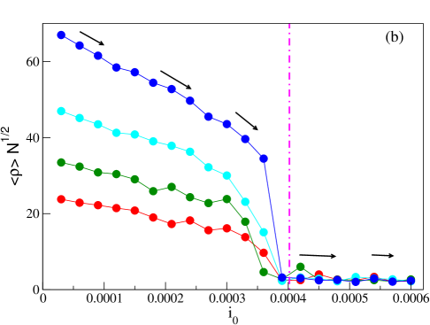
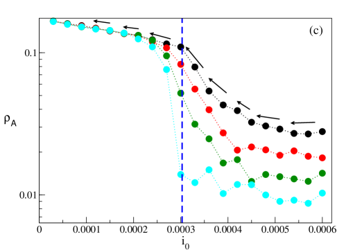
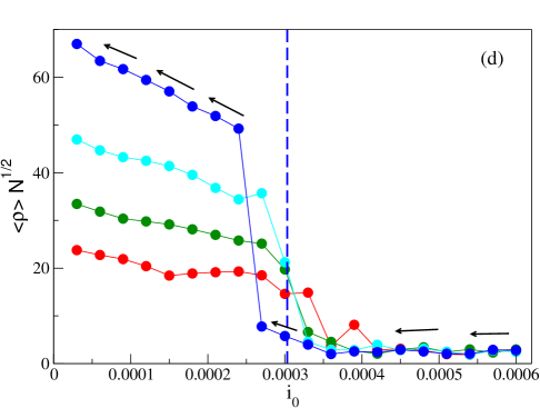
Figure 8: (a,c) Average order parameter $\rho_{A}$ versus $i_{0}$ for different system sizes: $N=10000$ (black circles), 20000 (red circles), 40000 (green circles) and 80000 (cyan circles). The values of $\rho_{A}$ have been averaged over 5-20 network realizations for a time interval $t_{E}=20-30$ s following a transient of $t_{T}=20-30$ s. (b,d) Order parameter $\langle\rho\rangle$ for a single network realization multiplied by $\sqrt{N}$ versus $i_{0}$ for different network sizes. The sizes are identified by the same symbols as in panel (a) apart $N=160000$ (blue circles). The parameter $\rho$ has been averaged in time for a time interval $t_{E}=20$ s following a transient of $t_{T}=60$ s and refers to a single network realization. The magenta dash-dotted line in (a) and (b) is the SNB numerically estimated via finite size scaling analysis of $\rho_{A}$, while the blue dashed line in (c-d) is the sub-critical HB obtained from the CMF approach. All data refer to quasi-adiabatic simulations of QIF networks with $g_{0}=1$ for fixed in-degree $K=100$ by varying $i_{0}$: the data in (a) and (b) (in (c) and (d)) have been obtained by increasing (decreasing) $i_{0}$ in steps $\Delta i_{0}=0.00003$.

The bifurcations reported in Fig. 7 (a) have been identified as a sub-critical HB and a SNB of limit cycles, since they were associated to a hysteretic transition from asynchronous to oscillatory dynamics. The sub-critical HB, as identified from the CMF approach, is located at $i_{0}^{(HB)}\simeq 0.00303$, while the SNB at $i_{0}^{(SN)}\simeq 0.0040(1)$ has been identified numerically by finite size scaling of the order parameter $\rho_{A}$ as explained in the following.

It is known that sub-critical HBs (SNBs of limit cycles) are characterized by an abrupt transition from an asynchronous to an oscillatory state (from an oscillatory to a stationary state), however from the Fig. 7 (a) both transition appear as smoothed over a finite interval of the current $i_{0}$. This is due to two facts: 1) in the present case the asynchronous regime corresponds to a focus, therefore damped oscillations forced by finite size fluctuations are present in the asynchronous state; 2) the indicator $\rho_{A}$ is averaged over different network realizations. This average allows us to give a better estimate of the transition points, however it has also the drawback to smooth out the transition over a finite interval, since different networks will have slightly different transition points. However, we expect that for increasing system sizes the transition region will become narrower, since the network realization will be less statistically different and finite size fluctuations will decrease.

Let us describe in details the finite size analysis we have performed. As a first analysis we consider $\rho_{A}$ versus $i_{0}$ as obtained by quasi-adiabatic simulations by increasing (decreasing) $i_{0}$ from the value $6\times 10^{-5}$ ($6\times 10^{-4}$) to $6\times 10^{-4}$ ($6\times 10^{-5}$) in steps of $\Delta i_{0}=3\times 10^{-5}$ for system sizes $N=10000$, 20000, 40000 and 80000 (the data are shown in Fig. 8 (a) and (c)). It is evident from the figures that the transition region shrinks for increasing $N$ and at the same time for $i_{0}>i_{0}^{(SN)}$ ($i_{0}>i_{0}^{(HB)}$) the value of the parameter decreases drastically with $N$ indicating that the dynamics above such current is asynchronous. On the other hand for $i_{0}<i_{0}^{(SN)}$ ($i_{0}<i_{0}^{(HB)}$) $\rho_{A}$ either remains essentially constant or does not present a clear decrease with $N$, in this range of currents we can affirm that we have a coherent behaviour characterized by GOs. Furthermore by increasing $N$ the jumps of the order parameter at the transition become higher and steeper, but still at $N=80000$ they seem not to be abrupt. As previously stated, we believe that the origin of this smoothing is related not only to the finite size effects, but also to the fact that $\rho_{A}$ is obtained as an average over different network realizations, typically presenting slightly different values of the bifurcation points $i_{0}^{(SN)}$ and $i_{0}^{(HB)}$.

To verify this conjecture we have considered the time average of the indicator $\langle\rho\rangle$ for only one realization of the network and for systems sizes increasing from $N=20000$ to $N=160000$, the results of this analysis are reported in Fig. 8 (b) and (d). To make more evident the transitions we have now reported $\langle\rho\rangle$ multiplied by $\sqrt{N}$ in the figures, in this case for increasing $N$ one will observe an almost constant (growing) value of $\langle\rho\rangle\sqrt{N}$ for asynchronous (oscillatory) dynamics. As a matter of fact, in Fig. 8 (b) we observe that for $i_{0}\leq 0.00039<i_{0}^{(SN)}$ the quantity $\langle\rho\rangle\sqrt{N}$ grows as $N^{1/2}$, while above such value it is almost constant. Furthermore, at $N=160000$ we see an abrupt transition from a value $\langle\rho\rangle\sqrt{N}\simeq 34$ at $i_{0}=0.00036$ to a value $\langle\rho\rangle\sqrt{N}\simeq 2$ at $i_{0}=0.00039$. Similar effects are observable in Fig. 8 (d) where the sub-critical Hopf is characterized, and also in this case at $N=160000$ the jump from asynchronous to oscillatory dynamics is abrupt. Furthermore, the single realization gives values of the bifurcation points slightly different from that obtained from the analysis of the average $\rho_{A}$ as expected. These indications are consistent with the interpretation we have given of the smoothing of the transitions observable in this case over a finite interval of $i_{0}$ and of the lack of abrupt variations of the measured order parameter.

IV.2 Frequency range of the global oscillations

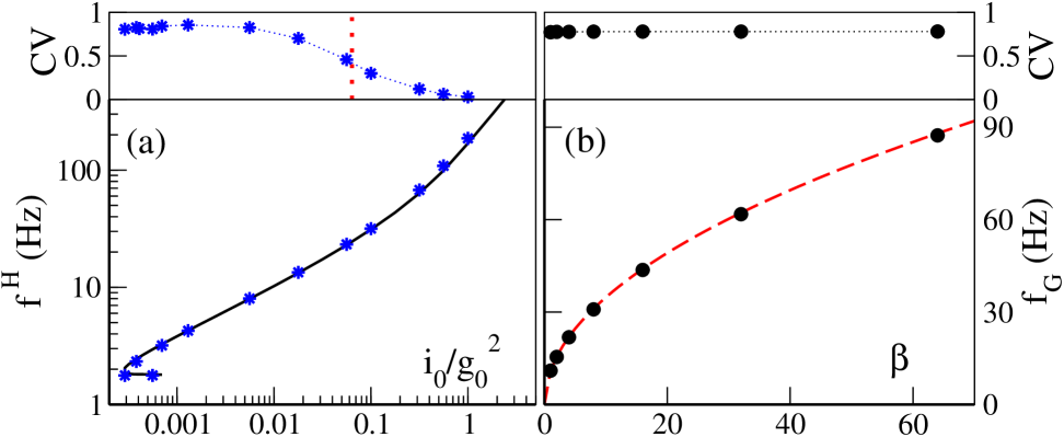
Figure 9: (a) Frequency $f^{H}$ of the GOs at the HB versus $i_{0}/g_{0}^{2}$: symbols are simulations for $N=20000$ and the solid line is the CMF result. (b) Frequency $f_{C}$ of the GOs as a function of the parameter $\beta$, where $i_{0}=\beta\times 0.01$, $g_{0}=\sqrt{\beta}$, $K=200$. Circles are network simulation data with $N=20000$ and the red dashed line represents the curve $\nu_{GO}=11\sqrt{\beta}$ Hz. The corresponding population averaged coefficients of variation CVs are shown above the two panels with the same symbols employed to denote simulation data. The vertical red dotted line shown in the upper part of panel (a) is the critical value defined in Di Volo et al. (2022) within the DA for the emergence of fluctuation-driven balanced asynchronous dynamics (for more details see the text). All data have been obtained by considering a time interval $t_{E}=100$ s, after discarding a transient of $t_{T}=20$ s. In (a) we set $g_{0}=1$.

At the HBs, GOs emerge with a frequency $f^{H}$ that is reported as a function of $i_{0}/g_{0}^{2}$ in Fig. 9 (a). The comparison between the CMF results (solid line) network simulations with $N=20000$ (blue stars) is very good along the whole bifurcation line predicted by the CMF. Furthermore, $f^{H}$ covers a wide range of frequencies ranging from $1.77$ Hz ($\delta$ band) to $\simeq 100$ Hz ($\gamma$ band), according to the usual classification of the brain rhythmsBuzsaki (2006). As visible in the upper part of the panel the population averaged coefficient of variation $CV$ is significantly greater than zero for $i_{0}/g_{0}^{2}<0.1$, where, as previously discussed, the firing activity is driven by fluctuations, as expected in the balanced regime. The fluctuation-driven regime is associated to quite high values of the ratio $R_{G}\simeq 6-11$, indicating that only $9-16\%$ of neurons participates to each population burst and that their activity is definitely slower than the collective one. Instead, in the mean-driven regime $R_{G}\to 2$ indicating that we observe the emergence of a peculiar cluster synchronization characterized by two groups (clusters) of neurons alternating their participation to the population bursts with low irregularity. This dynamics is quite similar to the one recently reported in Feld et al. (2024) for globally coupled QIF networks subject to additive Gaussian noise. Furthermore, across the examined range, $R_{0}\simeq 0.9-1$, suggesting that the GOs are associated to those neurons receiving few/no inhibitory PSPs during the global oscillation period.

As predicted by the CMF, the same dynamics should be observable at fixed $K$ by maintaining the ratio $i_{0}/g_{0}^{2}$ constant. We verified this by considering a state in the oscillatory regime corresponding to $(K,i_{0}/g_{0}^{2})=(200,0.01)$ and by varying, as a function of a control parameter $\beta$, the synaptic coupling and the current as $g_{0}=\sqrt{\beta}$ and $i_{0}=\beta\times 0.01$, while $K$ stays constant. In particular, we observed irregular dynamics characterized by an average $\overline{CV}\simeq 0.78$, as shown in the upper part of Fig. 9 (b), associated to GOs in the whole examined range $\beta\in[1,64]$. As expected, only the time scale varies, decreasing as $1/\sqrt{I}$, as previously shown, consequently the frequency $f_{G}$ of the GOs grows proportionally to $\sqrt{\beta}$ (as shown in Fig. 9 (b)) as well as the population average of the firing rates $F$. Obviously, the ratio of the two frequencies remains constant, in the present case the ratio $R_{G}\simeq 7.05$ indicating that one has always a slow firing activity of the neurons with respect to the GOs. Moreover, also $R_{0}$ stays almost constant around $\simeq 0.91$ implying that the frequency of the GOs essentially coincides with the frequency of the free neuron $\nu_{0}$ (2), Thus one can observe GOs with the same dynamical features in a wide frequency range by simply varying the parameter $\beta$.

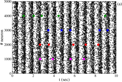
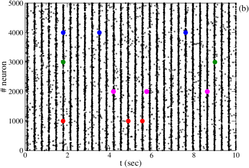
Figure 10: Raster plots of 5000 neurons for $K=10$ (a) and $K=250$ (b). In both cases the firing times of 4 neurons are evidenced by colored circles. Parameters $g_{0}=1$, $i_{0}=0.00055$, and $N=20000$.

IV.3 Two different types of GOs

As previously mentioned, we can identify two classes of GOs induced by discrete synaptic events in the interval $i_{0}/g_{0}^{2}\in[0.00036:0.00070]$. These two classes correspond to GOs observed at sufficiently low $K$ and high $K$, in particular for $i_{0}/g_{0}^{2}=0.00055$, we have the first type for $K\leq 30$ and the second one for $K\geq 200$, and asynchronous dynamics at intermediate in-degrees (as shown in Fig. 6). Raster plots corresponding to $K=10$ ($K=250$) are reported in Fig. 10 (a) (Fig. 10 (b)). The GOs are characterized by sparser (less synchronized) activity at low $K$, while at higher $K$ the neurons contributing to the population bursts fire almost at the same moment, with few outliers. However, the neurons participate in a quite random manner to the bursts in both cases (see the red circles in Fig. 10). Since the percentage of neurons contributing to a burst is $25\%$ (since $R_{G}=4$) for $K=10$ and $10\%$ for $K=250$ (here $R_{G}=9.6$), in the first case each neuron takes part in many more bursts than in the second case.

Moreover, GOs at $K\leq 30$ are associated to $R_{G}=4-7$, while those at $K\geq 200$ to much larger $R_{G}>10$, since $R_{G}$ grows with $K$, as evident from the lower panel of Fig. 11 (a) where data for $i_{0}/g_{0}^{2}=0.00055$ are reported for different values of $g_{0}=1$ (black circles) and $g_{0}=20$ (red stars). At the same time the spiking activity of the neurons is always quite irregular being $CV\simeq 0.75-0.92$ in all the examined range of $K$ both in the asynchronous and in the oscillating regime and for $g_{0}=1$ and $g_{0}=20$, as shown in the upper panel of Fig. 11 (a).

As shown in Fig. 11 (b) and as noticed in the previous sub-section, the frequency of the GOs $f_{G}$ is well approximated by the frequency of the free neuron $\nu_{0}$ (2), both for $g_{0}=1$ (lower panel) and $g_{0}=20$ (upper panel). The only difference among these two cases being the range of explored frequencies: for $g_{0}=1$ the frequencies are in the $\delta$-range between 1-4 Hz, smaller than 2 Hz for $K\leq 30$ and among 3-4 Hz for $K>200$, while for $g_{0}=20$ the frequencies are slow $\gamma$ ($<40$ Hz) for $K\leq 30$ and fast $\gamma$ ($60-80$ Hz) for large $K$ Colgin and Moser (2010).

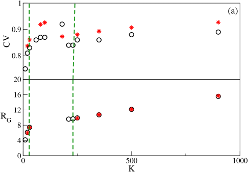
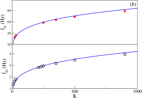
Figure 11: (a) $R_{G}$ versus $K$ in the lower panel, while in the upper panel is reported the population averaged coefficients of variation $CVs$ versus $K$. The green dashed lines refer to the HBs found within the CMF: GOs are expected for $K\leq 28$ and $K\geq 230$ in this case. (b) $f_{G}$ versus $K$, the blue solid lines denote $\nu_{0}$. Parameters $g_{0}=1$, $i_{0}=0.00055$, and $N=40000$ for the empty black circles, $g_{0}=20$, $i_{0}=0.22$, and $N=20000$ for the red stars.

The difference among these two GOs becomes clearer by considering the mean-field membrane potential evolution $V_{0}(t)$ given by the following zeroth-order Langevin equation:

$$\dot{V_{0}}(t)=V_{0}^{2}+\sqrt{K}[i_{0}-g_{0}\nu(t)]=V_{0}^{2}+A(t)\qquad;$$ (52)

where $A(t)$ is the effective input current, $\nu(t)$ is the population firing induced by the shot-noise and where current fluctuations have been neglected. Whenever $A<0$ ($A>0$) the QIF neuron will display excitable dynamics (periodic firing) Gutkin (2022).

The GOs reported in Fig. 6 (c) corresponding to $K=10$ are characterized by $A(t)$ always negative, while the GOs shown in Fig. 6 (d) for $K=210$ display an effective current that is positive for a large part of the oscillation period, as shown in Fig. 12 (a) and Fig. 12 (b), respectively. Therefore, for $K=10$ $V_{0}(t)$ displays sub-threshold oscillations, while for $K=210$ it has large excursions from negative to positive values driven by $A(t)>0$, as evident from the signal denoted by the black solid line in Fig. 12 (c) and Fig. 12 (d), respectively. In the same figures we report the time evolution of the membrane potential $v_{i}(t)$ of 4 generic neurons (characterized by colored lines), it is immediately evident that low (high) in-degree GOs are characterized by a low (high) level of coherence among the neurons. For $K=210$ the single neurons $v_{i}(t)$ essentially follow the men-field evolution $V_{0}(t)$ for a large part of the evolution. However, current fluctuations induce irregular firings of the neurons in proximity of the threshold, indeed $CV\simeq 0.85$. In contrast the dynamics of the neurons is quite uncorrelated over the whole evolution from reset to threshold for $K=10$ and also in this case the coefficient of variation is reasonably large $CV\simeq 0.75$.

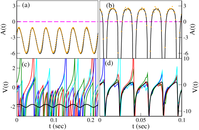
Figure 12: (a-b) Effective input currents $A(t)$ versus time : black lines (orange dots) refer to CMF (network simulations) results. (c-d) Membrane potential evolution in time: black lines (other colors) refer to $V_{0}(t)$ (single neuron dynamics). Data correspond to $i_{0}/g_{0}^{2}=0.00055$ (with $g_{0}=20$) and to $K=10$ (a-c), $K=210$ (b-d), network simulations realised for $N=80000$

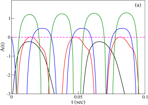
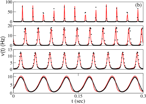
Figure 13: (a) Effective input currents $A(t)$ versus time : black line ($K=10$), red line ($K=60$), blue line ($K=100$) and green line $K=250$. (b) Population firing rates $\nu(t)$ versus time the panels from bottom to top refer to $K=10$, $K=60$, $K=100$ and $K=250$. Solid lines are CMF results obtained via the integration of Eq. (7), black symbols denote network simulation for $N=80000$. Data correspond to $i_{0}/g_{0}^{2}=0.00027$ (with $g_{0}=20$).

These behaviours can be somehow explained by 2 different mechanisms once remembering that for both cases the GO frequency $f_{G}$ is extremely close to the firing frequency of an isolated neuron $\nu_{0}=1/T_{0}$. This suggests that at a first approximation the GOs are due to the neurons not receiving any inhibitory PSP from reset to threshold. For low $K$, whenever a neuron fires large amplitude inhibitory PSPs are delivered, since their amplitude is $g_{0}/\sqrt{K}$. These lead the membrane potentials of the $K$ post-synaptic neurons to have quite similar values, and therefore the pre-synaptic neuron spiking induces a transient synchronization of the $K$ post-synaptic neurons. A sub-group of these, not receiving any further PSPs, can eventually reach threshold together at a time $\simeq T_{0}$. This transient synchronizing effect of small clusters of neurons (termed cluster activation) is at the origin of the GOs observable for $K=10$. For increasing $K$, the amplitude of the PSPs decreases, therefore above some critical in-degree ($K\simeq 30$ in this case) a single inhibitory PSP is no longer able to induce a sufficiently strong synchronizing effect on the post-synaptic neurons and the dynamics become asynchronous (as shown in Fig. 6 (c) (blue line)).

For larger $K$, the post-synaptic neurons receive many small inhibitory PSPs at each population burst, whenever $K$ is sufficiently large a non negligible part of the neurons can get synchronized by the discharge of inhibitory PSPs. As shown in Fig 13 (d), the time courses of the membrane potentials are now extremely coherent by approaching the threshold, where fluctuations lead to irregular firing of the neurons. However, a sufficient percentage of these drift-driven neurons is always able to fire together with a period $\simeq T_{0}$ giving rise to the GOs.

The one described above is the scenario in the interval $i_{0}/g_{0}^{2}\in[0.00036:0.00070]$, where for fixed $i_{0}/g_{0}^{2}$ one has GOs at low and large $K$ separated by a region of intermediate $K$ where the dynamics is asynchronous. For larger $i_{0}/g_{0}^{2}>0.00070$ we have only drift-driven GOs, since oscillatory dynamics is observable only for sufficiently large $K$. At low $K$ either the value of $g_{0}$ is too small to promote transient synchronization among the post-synaptic neurons or the period $T_{0}=\pi/\sqrt{I}=\pi/\sqrt{i_{0}\sqrt{K}}$ becomes too long to allow the cluster of post-synaptic neurons to reach threshold without receiving other PSPs.

However, it is unclear what happens for $i_{0}/g_{0}^{2}<0.00036$, in this region there are GOs for any value of the in-degree, as shown in Fig. 5 (a). The main question is if we pass from one mechanism to the other in a continuous or discontinuous way. Therefore, we have analyzed in detail the behaviour in this region by fixing $i_{0}/g_{0}^{2}=0.00027$ and by exploring the collective dynamics at different in-degrees. In Fig. 13 (a) we report for various $K$ the effective current $A(t)$ obtained within the CMF approach, estimated via the integration of Eq. (7) with the pseudo-spectral methods (see Appendix C for more details). From the figure it is evident that $A(t)$ begins to become partially positive for $K\geq 60$, therefore we could speak of the cluster activation mechanism for lower $K$ and of the drift-driven mechanism for larger $K$. At the same time the neurons become more and more synchronized within each population burst, as shown in Fig. 13 (b), thus indicating that the effect of a positive $A(t)$ leads them to be more and more coherent as expected. Despite the number of neurons participating to a population burst declines with $K$, analogously to what seen already for $i_{0}/g_{0}^{2}=0.00055$, indeed $R_{G}$ passes from value 4 at $K=10$ to value 10 at $K=250$. At the same time the firing activity remains always irregular with $CV\simeq 0.75-0.85$ in the whole examined range. However, all the indications suggest that the transition from one type of GO to the other occurs smoothly by increasing $K$ in this case.

V Summary and Discussion

In this paper we have presented a mean-field theory for balanced QIF neural networks encompassing synaptic Poisson noise and sparsity in the network connections. This approach, termed Complete Mean-Field (CMF), has allowed us to perform linear and weakly non-linear stability analysis of the asynchronous state, revealing sub- and super-critical Hopf instabilities leading to global oscillations (GOs). Therefore, besides asynchronous and oscillatory regimes, there is also a region of co-existence of these two solutions near the hysteretic transitions associated with the sub-critical Hopf bifurcations. As a further result of this analysis it emerges that the phase diagram depends only on two parameters: the in-degree $K$ (number of pre-synaptic neurons) and the ratio $i_{0}/g_{0}^{2}$ between the external excitatory drive and the square of the synaptic coupling. A peculiarity of the Hopf bifurcation line is that it is re-entrant at low $i_{0}/g_{0}^{2}$: in a limited range of $i_{0}/g_{0}^{2}$ one has GOs at low $K$ and high $K$-values, and asynchronous dynamics at intermediate in-degrees. Furthermore, the GOs observable at low and high $K$, despite being both associated with the irregular firing of single cells, are promoted by two different mechanisms: ”cluster activation” at low in-degree and a ”drift-driven” mechanism at high in-degree.

The network dynamics is well captured by the CMF, but not by the diffusion approximation (DA) Di Volo et al. (2022) valid in the limit of small PSPs (large $K$) and high neuronal activity (large $i_{0}$ and/or small $g_{0}$). Indeed, the DA works well for large $i_{0}/g_{0}^{2}>0.5$, but fails at low $i_{0}/g_{0}^{2}$ where it is completely unable to reproduce the scenario. In particular, the DA predicts the emergence of GOs only via super-critical Hopf bifurcations and that in the limit $i_{0}/g_{0}^{2}\to 0$ the critical in-degree $K_{c}$ required to observe GOs should diverge to infinity. Instead, at sufficiently low $i_{0}/g_{0}^{2}<0.00036$ GOs are observable for any $K$ value, as predicted by the CMF and in agreement with simulations.

An intermediate approximation going in the direction of the CMF can be obtained by considering an expansion to the third order of the source term in the continuity equation. This gives rise to the D3A approximation that we have studied in this paper. This approximation also predicts the emergence of GOs only via super-critical Hopf bifurcations and it is unable to reproduce the re-entrant Hopf bifurcation line found within the CMF. On the positive side, D3A captures well the network dynamics already for $i_{0}/g_{0}^{2}>0.02$ (i.e. for a parameter value an order of magnitude smaller than the DA) and it forecasts correctly that the GOs are present for sufficiently low $i_{0}/g_{0}^{2}$ for any in-degree, even if it gives a higher bound for this value with respect to CMF.

To understand the mechanisms responsible for the emergence of GOs at sufficiently low and high in-degree one should consider the effective input current $A(t)$ driving the mean-field dynamics in the two cases: at low $K$ $A(t)$ always induces sub-threshold dynamics, while at large $K$ this is mostly supra-threshold. In the first case GOs are promoted by small groups of neurons transiently synchronized by a large inhibitory PSP traveling together towards threshold, without being affected by further inhibitory PSPs. This is the origin of the name of the mechanism: ”cluster activation”. At large $K$ a large part of neurons, highly synchronized due to the previously received barrage of small inhibitory PSPs, are ”drift driven” towards the threshold by the positive effective input current, however only a small part of them, receiving few or no PSPs, will reach threshold almost at the same time giving rise to the GO. The Hopf bifurcations leading to these two types of GOs are characterized by distinct features. For large $K$ the collective dynamics is clearly dominated by the two most unstable (complex conjugate) eigenvalues. At low $K$, the spectrum is not only characterized by a pair of complex-conjugate eigenvalues responsible for the instability, but also by additional undamped pairs of eigenvalues that lie very close to the unstable ones. This suggests that, in this case, the instability is no longer controlled only by the two most unstable modes, but also by additional modes, which contribute to the coherent dynamics. Indeed, the population bursts are not generated by highly synchronized neurons, as is the case at high in-degrees.

From analytic investigations performed within the DA in Di Volo et al. (2022), it emerges that the asynchronous balanced dynamics could be either fluctuation-driven (mean-driven) for sufficiently small (large) values of $i_{0}/g_{0}^{2}$ Lerchner et al. (2006); Renart et al. (2007). Indeed, we have verified that in a large region of the phase space (namely, for $i_{0}/g_{0}^{2}<0.1$) the single neuron dynamics remains highly irregular, characterized by $CV>0.75$, regardless of the in-degree and whether the global activity is asynchronous or oscillatory.

As mentioned in the Introduction, this paper can be considered as the natural completion of the DA analysis reported in two well-known papers devoted to the emergence of GOs in sparse inhibitory Brunel and Hakim (1999) and excitatory-inhibitory neural networks Brunel (2000). However, the model we consider is the quadratic integrate-and-fire, while the one analyzed in Brunel and Hakim (1999); Brunel (2000) is the leaky integrate-and-fire. As already reported in di Volo and Torcini (2018), GOs can be observed in QIF sparse networks even for instantaneous synapses in the absence of any synaptic delay. This is not the case for LIF. Indeed, for inhibitory LIF networks the period of GOs is two/three times the synaptic delay (assumed to be on the order of few ms), thus the observable frequencies $f_{G}$ are limited to a range of 100-200 Hz. Instead, in our case $f_{G}$ can range from the $\delta$-band (0.5-3.5 Hz) to the $\gamma$-range (30-100 Hz), being $f_{G}$ essentially proportional to the square root of the external excitatory drive $I$. One would naively expect that slow GOs observable for low $I$ are associated with irregular spiking dynamics, while fast GOs at high $I$ are linked to almost regular neuronal spiking. However, the microscopic dynamical behaviour (fluctuation-driven or mean-driven) is controlled by the value of the ratio $i_{0}/g_{0}^{2}$. Irregular or regular spiking is observable at fixed in-degree $K$ by maintaining the ratio constant, the only effect of rescaling $i_{0}$ and $g_{0}$ being the modification of the time scale of the model. Therefore, GOs of any frequency (fast or slow) can be obtained by conveniently rescaling $i_{0}$ and $g_{0}$ with either irregular or regular firing.

In Brunel (2000), Brunel, by considering an excitatory-inhibitory network in the inhibition-dominated regime was able to identify slow ($f_{G}\simeq 20-60$ Hz) and fast ($f_{G}\simeq 120-180$ Hz) GOs separated by an asynchronous regime. This scenario closely resembles the one we have identified at low $i_{0}/g_{0}^{2}$. However, the analysis in Brunel (2000), besides considering excitatory and inhibitory neurons, is performed within the DA, and for purely inhibitory networks only fast oscillations have been reported in Brunel and Hakim (1999). Furthermore, the frequency of the slow (fast) oscillations is controlled by the membrane time constant (synaptic time scale) while in our case it is always related to the external excitatory drive. As a further difference, the parameter $R_{G}$ (which is the ratio of $f_{G}$ with respect to the population firing rate) takes values around 3-4 in both the slow and fast oscillation regimes, while in our case $R_{G}\simeq 4-6$ for low $K$ and $R_{G}>10$ for high $K$. Therefore, it is worth extending our approach to excitatory-inhibitory networks in order to understand in more detail the origin of these differences and similitudes and to investigate how the scenario will be modified by the presence of excitatory neurons.

Our theoretical results are rigorously derived for the continuity equation (7) obtained in the thermodynamic limit $N\to\infty$. This equation is valid even for a finite network as long as (i) the firing events of the pre-synaptic neurons can be treated as independent and (ii) all emitting and receiving neurons can be considered to be statistically equivalent. This introduces a lower and upper bound on the in-degree $K$. On one side, the network must be sparse, $K\ll N$, otherwise, the pre-synaptic spike trains will no longer be independent. On the other side, for the statistical equivalence any neuron should be connected to any other (no closed loop should emerge) and this is achieved in an Erdös-Renyi network, analogous to the set-up we considered, when the in-degree is larger than the percolation threshold, i.e. $K>1$ Albert and Barabási (2002). The role of finite $N$ effects for the macroscopic behaviour of sparse LIF networks has been considered in Brunel and Hakim (1999); Brunel (2000) and more recently in Klinshov and Kirillov (2022); Klinshov et al. (2023) for globally coupled QIF networks. Future studies should be devoted to the inclusion of finite size effects in the framework of the CMF for balanced neural networks.

As stated above, GOs with tunable frequencies can emerge even in extremely sparse inhibitory networks thanks to the mechanism of ”cluster activation”. This mechanism can be at the basis of the $\gamma$-oscillations observed in the hippocampus and generated by a population of interneurons with low in-degree $K\simeq 30-80$ Sik et al. (1995); Buzsáki and Wang (2012).

Clustering instabilities observed in globally coupled neural networks in the presence of additive noise for LIF Brunel and Hansel (2006) and QIF neurons Feld et al. (2024) should not be confused with the mechanism of ”cluster activation” here reported. The dynamics induced by the clustering instability is characterized by GOs with a frequency that is a multiple of the single neuron frequency and by low irregularity in the firing activity, whereas the GOs emerging due to the ”cluster activation” mechanism exhibit stochastic synchrony (in contrast to regular synchrony where neurons resonantly lock with the oscillatory input) with associated high values of the coefficient of variation $CV\simeq 0.75-0.85$ denoting a quite irregular firing activity. Clustered dynamics can be observed in this model only in the mean-driven regime, for large $i_{0}/g_{0}^{2}>0.1$ and large $K>200$. The clustered phase is characterized by population bursts where neurons are split in two equally populated clusters firing in alternation. Although the global activity appears regular, the single neurons display switching between the two clusters due to fluctuations in the input currents, but with a low level of irregularity in their dynamics. This clustering phenomenon has been already reported for heterogeneous and homogeneous globally coupled QIF networks subject to weak additive noise Feld et al. (2024).

As shown in Appendix D, the introduction of finite synaptic times does not alter substantially the scenario here depicted for instantaneous synapses. Indeed, also in this case for sufficiently low $i_{0}/g_{0}^{2}$ and $K$, the DA is unable to capture the network dynamics and the inclusion of discrete synaptic events is fundamental in order to reproduce the network simulations. These results call for the inclusion in the CMF of more biologically realistic features, such as the delay in the pulse transmission or the finite duration of the PSPs. These generalizations are technically feasible, however they require a careful derivation that goes beyond the scopes of the present analysis and that will be reported in future studies.

Appendix A Event driven simulations of the QIF network

The QIF network model (1) can be integrated by employing an event driven method, since we always considered supra-threshold neurons $I>0$ Tonnelier et al. (2007). In particular, the method consists in integrating exactly the network evolution between one spike emitted by neuron $j$ at time $T_{1}=t^{(n)}_{j}$ and the next one emitted by the $q$-th neuron at time $T_{2}=t^{(n+1)}_{q}$.

The first step consists in identifying the next firing neuron, therefore one should evaluate the time ${\cal T}_{i}$ needed to each neuron $i$ to reach the firing threshold $v_{th}=+\infty$. These times can be evaluated on the basis of the value of the neuron membrane potential at time $T_{1}^{+}$ (immediately after the spike emission), as follows:

$${\cal T}_{i}(n+1)=\frac{1}{\sqrt{I}}\left[\frac{\pi}{2}-\arctan\left(B_{i}(T_{1}^{+})\right)\right]\qquad{\rm where}\qquad B_{i}(t)\equiv\frac{v_{i}(t)}{\sqrt{I}}\enskip.$$ (53)

The next firing neuron $q$ will be the one associated with the smallest time ${\cal T}_{q}(n+1)$ and the next firing time will be $T_{2}=T_{1}+{\cal T}_{q}(n+1)$.

Once the next firing neuron is identified, the membrane potential evolution between $[T_{1}^{+},T_{2}^{-}]$ is given by

$$v_{i}(T_{2}^{-})=\sqrt{I}\tan\left(\frac{T_{2}-T_{1}}{\sqrt{I}}+B_{i}(T_{1}^{+})\right)$$ (54)

and the membrane potentials of the post-synaptic neurons connected to neuron $q$ should be modified as follows, due to the spike arrival,

$$v_{k}(T_{2}^{+})=v_{k}(T_{2}^{-})-g\qquad{\rm if}\qquad k\in{\rm post}(q)\enskip;$$ (55)

while the others are left unchanged. At this point the adjoint variables $B_{i}(T^{+}_{2})$ are evaluated by following their definition, apart the one associated to the spiking neuron $q$ that it is simply set to $B_{q}(T^{+}_{2})=-\pi/2$ due to the reset condition for the membrane potential (namely, $v_{q}(T^{+}_{2})=-\infty$). The iterative procedure can be now repeated to find the next firing neuron and so on.

See also Engelken (2023) for a recently developed efficient event-driven simulations scheme for sparse random networks.

Appendix B Integration of the Langevin equations

Regarding the integration of the mean-field Langevin equation (6), we considered $N=20000-80000$ replica of such equation, corresponding to $N$ uncoupled QIF neurons. In particular, we integrated such $N$ uncoupled evolution equations (6) by employing an Euler integration scheme with $\Delta t$. The population firing rate $\nu(t)$ entering in Eq. (2) at time $t$ is estimated self-consistently by counting the number of spikes $N_{sp}(\Delta t)$ emitted by the $N$ neurons in the preceding time window $T_{w}$, as follows:

$$\nu(t)=\frac{N_{sp}(\Delta t)}{T_{w}N}\quad.$$ (56)

For the shot-noise case, at the end of every time interval $T_{w}$, every neuron receives an inhibitory post-synaptic input of finite amplitude $g$ with a probability $K\times\nu(t)\times\Delta t$ mimicking a Poissonian process with rate $K\nu(t)$.

To simulate the Langevin evolution (6) within the DA, we considered $N$ uncoupled neurons whose membrane potential obeys the following stochastic differential equation

$$\dot{V}(t)=F(V)+I-g_{0}\sqrt{K}\nu(t)+g_{0}\sqrt{\nu(t)}\xi(t)$$ (57)

where $\xi$ is the normalized Gaussian white noise. The firing rate is estimated also in this case by the activity of the $N$ neurons via (56) by performing an average on a sliding time window of duration $T_{w}$ and the integration is performed again via an Euler scheme. We fixed $\Delta t=5\times 10^{-4}\tau_{m}$ and $T_{w}=0.005\tau_{m}$, and an initial transient time $t_{t}=10$ s is discarded in all the simulations.

Appendix C Integration of the continuity and Fokker-Planck equations

In order to integrate the CMF and the FPE we transformed the membrane potential $V$ in the angular variable $\theta=2\arctan V$ with $\theta\in[-\pi,+\pi]$, in the present case we used the standard transformation to pass from the QIF to the $\theta$-model.

Accordingly, the PDF $P(V,t)$ for the membrane potentials is related to the PDF $R(\theta,t)$ of the corresponding angular variables as follows

$$P(V,T)=(1+\cos\theta)R(\theta,t)\quad.$$ (58)

The CMF equation then takes the following form

$$\frac{\partial R(\theta,t)}{\partial t}=-\frac{\partial}{\partial\theta}\left[((I+1)+(I-1)\cos\theta)R(\theta,t)\right]+K\nu(t)\left[R(\theta^{+},t)\frac{1+\cos\theta^{+}}{1+\cos\theta}-R(\theta,t)\right]$$ (59)

where

$$\theta^{+}=2\arctan\left[\tan\left(\frac{\theta}{2}\right)+g\right]\quad.$$ (60)

By expanding the term within square brackets on the right-hand side in (59) up to the second order in $g$ we obtain the corresponding FPE in the angular space

$$\frac{\partial R}{\partial t}=-\frac{\partial}{\partial\theta}\left\{\left[(1-\cos\theta)+(A(t)+D(t)\sin\theta)(1+\cos\theta)\right]R-D(t)(1+\cos\theta)^{2}\frac{\partial R}{\partial\theta}\right\}$$ (61)

where $A(t)=\sqrt{K}[i_{0}-g_{0}\nu(t)]$, $D(t)=[g_{0}^{2}\nu(t)]/2$ and $R=R(\theta,t)$.

The Fokker–Planck formulation can be extended by including the third order term in the expansion, this amounts to add on the right-hand side of (61) the following term

$$H(t)\frac{\partial}{\partial\theta}\left[(1+\cos\theta)^{3}\frac{\partial^{2}R}{\partial\theta^{2}}-3\sin\theta(1+\cos\theta)^{2}\frac{\partial R}{\partial\theta}+(1+\cos\theta)(1-\cos\theta-2\cos^{2}\theta)R\right]$$ (62)

where $H(t)=\frac{g_{0}^{3}}{3!\sqrt{K}}\nu(t)$.

In all the cases listed above we assumed that the flux at the threshold determines the instantaneous population firing rate, therefore this sets the following boundary condition for the PDFs

$$\lim_{V\to\infty}V^{2}P(V,t)=2R(\pi,t)=\nu(t)\enskip.$$

C.1 Time splitting pseudo-spectral method

The above partial differential equations can be integrated by employing time-splitting pseudo-spectral methods developed for spatially extended systems, such as the complex Ginburg-Landau equation Torcini et al. (1997), surface growth models Torcini and Politi (2002) and asymmetrically coupled Swift-Hohenberg and Cahn-Hilliard equations Schüler et al. (2014). In particular, in order to perform the numerical integration we considered a discrete grid for the angular values of resolution $\Delta\theta$ and a discrete time evolution with a constant time step $\Delta t$. The discretized PDF can be written as $R(i,n)$, where the integer indices $i$ and $n$ represent the angular and temporal variables, respectively. Periodic boundary conditions are assumed for the PDF: $R(i,n)=R(i+I,n)$, where $I$ is the number of sites of the grid namely $2\pi=I\Delta\theta$.

In general the evolution equations for the PDF $R(\theta,t)$ can be rewritten as follows

$$\partial_{t}R(\theta,t)=({\cal L}+{\cal N})R(\theta,t)$$ (63)

where ${\cal L}$ and ${\cal N}$ are a linear and non-linear operator, respectively. For a sufficiently small time step $\Delta t$ the formal solution of (63) is the following

$$R(\theta,t+\Delta t)={\rm e}^{({\cal L+N})\Delta t}R(\theta,t)\quad.$$ (64)

The evolution operator appearing in (64) can be approximated via the Trotter formulas as follows

$${\rm e}^{({\cal L+N})\Delta t}\approx{\rm e}^{{\cal N}\Delta t/2}{\rm e}^{{\cal L}\Delta t}{\rm e}^{{\cal N}\Delta t/2}+{\cal O}(\Delta t^{3})\quad.$$ (65)

For a finite time interval $T=M\Delta t$ we can lump together $M-1$ integration steps and approximate the evolution operator over the interval $T$ as

$${\rm e}^{({\cal L+N})T}\approx{\rm e}^{{\cal N}\Delta t/2}\left({\rm e}^{{\cal L}\Delta t}{\rm e}^{{\cal N}\Delta t}\right)^{M-1}{\rm e}^{{\cal L}\Delta t}{\rm e}^{{\cal N}\Delta t/2}\quad;$$ (66)

this amounts to perform successive integration of the linear and non-linear part. The linear part

$$\partial_{t}R(\theta,t)={\cal L}R(\theta,t)$$ (67)

is usually solved in Fourier space where it takes the form

$$\partial_{t}{\tilde{R}}(p,t)=f(p){\tilde{R}}(p,t)$$ (68)

where ${\tilde{R}}(p,t)$ is the Fourier transform of the PDF $R(\theta,t)$ over the angular variable, $p$ is an integer defined in the interval $p\in[-I/2,I/2-1]$ representing the wave number and $f(p)$ is a polynomial in $p$. The time evolution for ${\tilde{z}}$ over a time step $\Delta t$ is given by

$${\tilde{R}}(p,t+\Delta t)={\rm e}^{f(p)\Delta t}{\tilde{R}}(p,t)\quad;$$ (69)

therefore the integration of (67) in the original space can be written as

$${\tilde{R}}(\theta,t+\Delta t)={\cal F}^{-1}{\rm e}^{f(p)\Delta t}{\cal F}{R}(\theta,t)\quad,$$ (70)

where ${\cal F}$ (${\cal F}^{-1}$) is the direct (inverse) Fourier transform.

The integration of the non-linear part amounts to solve

$$\partial_{t}R(\theta,t)={\cal N}R(\theta,t)$$ (71)

this can be integrated by employing some standard integration method, in the specific we have employed the Euler scheme, therefore the time evolution of the PDF is given by

$$R(\theta,t+\Delta t)=R(\theta,t)+[{\cal N}R(\theta,t)]\Delta t\quad.$$ (72)

In order to increase the precision of the integration, the angular derivatives of $R$ eventually entering in ${\cal N}R(\theta,t)$ have been evaluated in the Fourier space.

In the following we will explicitly report the linear and non-linear operators considered in the article.

C.1.1 The CMF

The linear operator for the CMF is the following

$${\cal L}R(\theta,t)=-(I+1)\frac{\partial R(\theta,t)}{\partial\theta}-K\nu(t)R(\theta,t)$$ (73)

and the non-linear one is

$${\cal N}R(\theta,t)=-\frac{\partial}{\partial\theta}\left[(I-1)\cos\theta R(\theta,t)\right]+K\nu(t)\left[R(\theta^{+},t)\frac{1+\cos\theta^{+}}{1+\cos\theta}\right]\quad.$$ (74)

The linear integration can be performed as in (70) with

$$f(p)=-K\nu(t)-(I+1){i}p$$

where ${i}$ is the imaginary unit.

C.1.2 The FPE

The linear operator for the FPE can be written as

$${\cal L}_{FP}R(\theta,t)=D(t)\left[R(\theta,t)+\frac{\partial^{2}R(\theta,t)}{\partial\theta^{2}}\right]-(1+A(t))\frac{\partial R(\theta,t)}{\partial\theta}$$ (75)

and the non-linear one as

$${\cal N}_{FP}R(\theta,t) = f(\theta,t)R(\theta,t)+g(\theta,t)\frac{\partial R(\theta,t)}{\partial\theta}+h(\theta,t)\frac{\partial^{2}R(\theta,t)}{\partial\theta^{2}}$$ (76)

$$f(\theta,t) = \sin\theta(A(t)-1)-D(t)(2\cos^{2}\theta+\cos\theta)$$ (77)

$$g(\theta,t) = \cos\theta(1-A(t))-3D(t)\sin\theta(1+\cos\theta)$$ (78)

$$h(\theta,t) = D(t)\cos\theta(2+\cos\theta)$$ (79)

The term needed for the linear integration appearing in (70) has the following expression

$$f(p)=D(t)(1-p^{2})-(1+A(t)){i}p$$

The extention to the third order is algebraically complicated, but straightforward, we do no report here the expressions of the linear and non-linear operators but they can be easily derived form Eqs. (61) and (62).

Appendix D Synaptic Filtering

In the paper we have always considered instantaneous synapses, however a fundamental question is if the introduction of finite synaptic times will alter the observed scenario. In particular, to generalize our findings we have considered a network of QIF neurons with exponentially decaying PSPs, this amounts to rewrite the model (1) as follows

$$\dot{v}_{i}(t) = v_{i}^{2}+I-gS_{i}(t)\quad i=1,\dots,N$$

$$\tau_{s}\dot{S}_{i}(t) = -S_{i}(t)+\sum_{j=1}^{N}\sum_{n}\varepsilon_{ji}\delta(t-t_{j}^{(n)})$$ (80)

where $S_{i}(t)$ represents the synaptic input current due to the linear super-position of the exponential PSPs emitted by the pre-synaptic neurons connected to neuron $i$ and $\tau_{s}$ is the synaptic decay time of the PSP.

We have considered the same case reported in Fig. 1 (b) in Goldobin et al. (2024), but this time the PSPs have a finite duration, namely $\tau_{s}=0.1\tau_{m}$. As shown in Fig. 14, analogously to what found for instantaneous synapses the DA (red line) fails in reproducing the network simulations (black line), while the inclusion of shot-noise in the Langevin dynamics allow to recover the correct evolution (violet line).

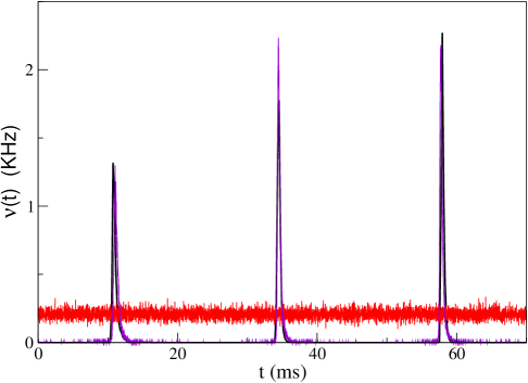
Figure 14: Population firing rates $\nu(t)$ versus time for exponentially decaying PSPs. The black line refers to network simulations with $N=20000$, while the red (violet) line to Langevin simulations for diffusive (shot-) noise with $N=20000$ uncoupled neurons. The data refer to QIF networks with exponentially decaying PSPs (80) with $K=200$, $i_{0}=0.16$, $g_{0}=4$, and $\tau_{s}=0.1\tau_{m}$.

Therefore we can conclude that for finite $\tau_{s}$ we find the same scenario reported for instantaneous synapses, the detailed investigation of the role of the synaptic filtering is devoted to future analysis.

References

- Schottky (1918) W. Schottky, Annalen der Physik 362, 541 (1918).
- Henry and Kazarinov (1996) C. H. Henry and R. F. Kazarinov, Reviews of Modern Physics 68, 801 (1996).
- Goncalves et al. (2023) B. Goncalves, T. Huillet, and E. Löcherbach, Advances in Applied Probability 55, 444 (2023).
- Kanazawa (2017) K. Kanazawa, Statistical mechanics for athermal fluctuation: Non-Gaussian noise in physics (Springer, 2017).
- Lucente et al. (2023) D. Lucente, M. Viale, A. Gnoli, A. Puglisi, and A. Vulpiani, Physical Review Letters 131, 078201 (2023).
- Lucente et al. (2025) D. Lucente, M. Baldovin, M. Viale, and A. Vulpiani, arXiv preprint arXiv:2504.05980 (2025).
- Fodor et al. (2018) É. Fodor, H. Hayakawa, J. Tailleur, and F. van Wijland, Physical Review E 98, 062610 (2018).
- Blanter and Büttiker (2000) Y. M. Blanter and M. Büttiker, Physics Reports 336, 1 (2000).
- Frisch and Lloyd (1960) H. Frisch and S. Lloyd, Physical Review 120, 1175 (1960).
- Capocelli and Ricciardi (1971) R. Capocelli and L. Ricciardi, Kybernetik 8, 214 (1971).
- Tuckwell (1988) H. C. Tuckwell, Introduction to theoretical neurobiology: nonlinear and stochastic theories, Vol. 2 (Cambridge University Press, 1988).
- Miles (1990) R. Miles, The Journal of Physiology 431, 659 (1990).
- Song et al. (2005) S. Song, P. J. Sjöström, M. Reigl, S. Nelson, and D. B. Chklovskii, PLoS Biology 3, e68 (2005).
- Buzsáki and Mizuseki (2014) G. Buzsáki and K. Mizuseki, Nature Reviews Neuroscience 15, 264 (2014).
- Lefort et al. (2009) S. Lefort, C. Tomm, J.-C. F. Sarria, and C. C. Petersen, Neuron 61, 301 (2009).
- Bi and Poo (1999) G.-q. Bi and M.-m. Poo, Nature 401, 792 (1999).
- Barbour et al. (2007) B. Barbour, N. Brunel, V. Hakim, and J.-P. Nadal, TRENDS in Neurosciences 30, 622 (2007).
- Kisvárday et al. (1993) Z. F. Kisvárday, C. Beaulieu, and U. T. Eysel, Journal of Comparative Neurology 327, 398 (1993).
- Sik et al. (1995) A. Sik, M. Penttonen, A. Ylinen, and G. Buzsáki, Journal of Neuroscience 15, 6651 (1995).
- Buzsáki and Wang (2012) G. Buzsáki and X.-J. Wang, Annual Review of Neuroscience 35, 203 (2012).
- Wildenberg et al. (2021) G. A. Wildenberg, M. R. Rosen, J. Lundell, D. Paukner, D. J. Freedman, and N. Kasthuri, Cell Reports 36 (2021).
- Richardson and Swarbrick (2010) M. J. E. Richardson and R. Swarbrick, Physical Review Letters 105, 178102 (2010).
- Iyer et al. (2013) R. Iyer, V. Menon, M. Buice, C. Koch, and S. Mihalas, PLoS Computational Biology 9, e1003248 (2013).
- Olmi et al. (2017) S. Olmi, D. Angulo-Garcia, A. Imparato, and A. Torcini, Scientific Reports 7, 1577 (2017).
- Angulo-Garcia et al. (2017) D. Angulo-Garcia, S. Luccioli, S. Olmi, and A. Torcini, New Journal of Physics 19, 053011 (2017).
- Droste and Lindner (2017) F. Droste and B. Lindner, Journal of Computational Neuroscience 43, 81 (2017).
- Richardson (2018) M. J. E. Richardson, Physical Review E 98, 042405 (2018).
- Richardson (2024) M. J. E. Richardson, Physical Review E 109, 024407 (2024).
- Buzsaki (2006) G. Buzsaki, Rhythms of the Brain (Oxford University Press, 2006).
- Singer (2018) W. Singer, European Journal of Neuroscience 48, 2389 (2018).
- Csicsvari et al. (1998) J. Csicsvari, H. Hirase, A. Czurko, and G. Buzsáki, Neuron 21, 179 (1998).
- Fisahn et al. (1998) A. Fisahn, F. G. Pike, E. H. Buhl, and O. Paulsen, Nature 394, 186 (1998).
- van Vreeswijk and Sompolinsky (1996) C. van Vreeswijk and H. Sompolinsky, Science 274, 1724 (1996).
- Brunel (2000) N. Brunel, Journal of Computational Neuroscience 8, 183 (2000).
- Brunel and Wang (2003) N. Brunel and X.-J. Wang, Journal of neurophysiology 90, 415 (2003).
- Geisler et al. (2005) C. Geisler, N. Brunel, and X.-J. Wang, Journal of neurophysiology 94, 4344 (2005).
- Bi et al. (2021) H. Bi, M. Di Volo, and A. Torcini, Frontiers in systems neuroscience 15, 752261 (2021).
- Whittington et al. (2000) M. A. Whittington, R. D. Traub, N. Kopell, B. Ermentrout, and E. H. Buhl, International journal of psychophysiology 38, 315 (2000).
- Mann and Paulsen (2007) E. O. Mann and O. Paulsen, Trends in neurosciences 30, 343 (2007).
- Brunel and Hakim (1999) N. Brunel and V. Hakim, Neural computation 11, 1621 (1999).
- Kadmon and Sompolinsky (2015) J. Kadmon and H. Sompolinsky, Phys. Rev. X 5, 041030 (2015).
- Monteforte and Wolf (2010) M. Monteforte and F. Wolf, Phys. Rev. Lett. 105, 268104 (2010).
- di Volo and Torcini (2018) M. di Volo and A. Torcini, Phys. Rev. Lett. 121, 128301 (2018).
- Di Volo et al. (2022) M. Di Volo, M. Segneri, D. S. Goldobin, A. Politi, and A. Torcini, Chaos: An Interdisciplinary Journal of Nonlinear Science 32, 023120 (2022).
- Goldobin et al. (2024) D. S. Goldobin, M. di Volo, and A. Torcini, Phys. Rev. Lett. 133, 238401 (2024).
- Ermentrout and Kopell (1986) G. B. Ermentrout and N. Kopell, SIAM Journal on Applied Mathematics 46, 233 (1986).
- Gutkin (2022) B. Gutkin, in Encyclopedia of computational neuroscience (Springer, 2022) pp. 3412–3419.
- Golomb (2007) D. Golomb, Scholarpedia 2, 1347 (2007).
- Clusella and Montbrió (2024) P. Clusella and E. Montbrió, Physical Review E 109, 014229 (2024).
- Haskell et al. (2001) E. Haskell, D. Q. Nykamp, and D. Tranchina, Network: Computation in Neural Systems 12, 141 (2001).
- Marcinkiewicz (1939) J. Marcinkiewicz, Mathematische Zeitschrift 44, 612 (1939).
- Gardiner (1997) C. W. Gardiner, Handbook of Stochastic Methods, 2nd ed. (Springer, Berlin, 1997).
- Ermentrout (2008) B. Ermentrout, Scholarpedia 3, 1398 (2008), revision #122134.
- Kralemann et al. (2007) B. Kralemann, L. Cimponeriu, M. Rosenblum, A. Pikovsky, and R. Mrowka, Physical Review E 76, 055201(R) (2007).
- Dolmatova et al. (2017) A. V. Dolmatova, D. S. Goldobin, and A. Pikovsky, Physical Review E 96, 062204 (2017).
- Kuramoto (2012) Y. Kuramoto, Chemical oscillations, waves, and turbulence, Vol. 19 (Springer Science & Business Media, 2012).
- Daido (1992) H. Daido, Progress of Theoretical Physics 88, 1213 (1992).
- Cox and Matthews (2002) S. M. Cox and P. C. Matthews, J. Comput. Phys. 176, 430 (2002).
- Permyakova and Goldobin (2025) E. V. Permyakova and D. S. Goldobin, J. Comput. Phys. 520, 113493 (2025).
- (60) For numerical calculations in the Maple package, whenever needed the length of the digital mantissa of the variables was increased significantly beyond digits (environmental variable ‘Digits’) in order to maintain this accuracy. We adopted the following technical criterion for accuracy: the elevations of the decimal mantissa length by and by a factor of induce the relative changes of the calculated quantity of interest below .
- Nayfeh (2024) A. H. Nayfeh, Introduction to perturbation techniques (John Wiley & Sons, 2024).
- Ullner and Politi (2016) E. Ullner and A. Politi, Physical Review X 6, 011015 (2016).
- Lerchner et al. (2006) A. Lerchner, C. Ursta, J. Hertz, M. Ahmadi, P. Ruffiot, and S. Enemark, Neural computation 18, 634 (2006).
- Feld et al. (2024) Y. Feld, A. K. Hartmann, and A. Torcini, New Journal of Physics 26, 063017 (2024).
- Colgin and Moser (2010) L. L. Colgin and E. I. Moser, Physiology 25, 319 (2010).
- Renart et al. (2007) A. Renart, R. Moreno-Bote, X.-J. Wang, and N. Parga, Neural computation 19, 1 (2007).
- Albert and Barabási (2002) R. Albert and A.-L. Barabási, Reviews of modern physics 74, 47 (2002).
- Klinshov and Kirillov (2022) V. V. Klinshov and S. Y. Kirillov, Physical Review E 106, L062302 (2022).
- Klinshov et al. (2023) V. Klinshov, P. Smelov, and S. Y. Kirillov, Chaos: An Interdisciplinary Journal of Nonlinear Science 33 (2023).
- Brunel and Hansel (2006) N. Brunel and D. Hansel, Neural Computation 18, 1066 (2006).
- Tonnelier et al. (2007) A. Tonnelier, H. Belmabrouk, and D. Martinez, Neural Computation 19, 3226 (2007).
- Engelken (2023) R. Engelken, Advances in Neural Information Processing Systems 36, 3638 (2023).
- Torcini et al. (1997) A. Torcini, H. Frauenkron, and P. Grassberger, Physical Review E 55, 5073 (1997).
- Torcini and Politi (2002) A. Torcini and P. Politi, The European Physical Journal B-Condensed Matter and Complex Systems 25, 519 (2002).
- Schüler et al. (2014) D. Schüler, S. Alonso, A. Torcini, and M. Bär, Chaos: An Interdisciplinary Journal of Nonlinear Science 24 (2014).