Compression versus Accuracy:
A Hierarchy of Lifted Models

Abstract

Probabilistic graphical models that encode indistinguishable objects and relations among them use first-order logic constructs to compress a propositional factorised model for more efficient (lifted) inference. To obtain a lifted representation, the state-of-the-art algorithm Advanced Colour Passing (ACP) groups factors that represent matching distributions. In an approximate version using $\varepsilon$ as a hyperparameter, factors are grouped that differ by a factor of at most $(1\pm\varepsilon)$. However, finding a suitable $\varepsilon$ is not obvious and may need a lot of exploration, possibly requiring many ACP runs with different $\varepsilon$ values. Additionally, varying $\varepsilon$ can yield wildly different models, leading to decreased interpretability. Therefore, this paper presents a hierarchical approach to lifted model construction that is hyperparameter-free. It efficiently computes a hierarchy of $\varepsilon$ values that ensures a hierarchy of models, meaning that once factors are grouped together given some $\varepsilon$, these factors will be grouped together for larger $\varepsilon$ as well. The hierarchy of $\varepsilon$ values also leads to a hierarchy of error bounds. This allows for explicitly weighing compression versus accuracy when choosing specific $\varepsilon$ values to run ACP with and enables interpretability between the different models.

7707

1 Introduction

Probabilistic graphical models (PGMs) allow for modelling environments under uncertainty by encoding features in random variables and relations between them in factors. Lifted or first-order versions of PGMs such as parametric factor graphs [17] and Markov logic networks [18] incorporate logic constructs to encode indistinguishable objects and relations among them in a compact way. Probabilistic inference on such first-order models becomes tractable in the domain size when using representatives for indistinguishable objects [16], a technique referred to as lifting [17]. Lifting has been used to great effect in probabilistic inference including lifting various query answering algorithms [1, 2, 8, 9, 19, 22] next to lifting queries [3, 20] or evidence [19, 21].

Advanced Colour Passing (ACP) is the state-of-the-art algorithm to get a first-order model from a propositional one, specifically turning FGs into parametric FGs, grouping factors with identical potentials [1, 13]. The newest version, $\varepsilon$-Advanced Colour Passing ($\varepsilon$-ACP), considers approximate indistinguishability, using a number $\varepsilon$ to group factors whose potentials differ by a factor of at most $(1\pm\varepsilon)$ and are therefore considered $\varepsilon$-equivalent, with $\varepsilon$ as a hyperparameter [14]. $\varepsilon$-ACP allows for compressing a propositional model to a larger degree with increasing $\varepsilon$, leading to better runtime for inference tasks. It also allows for computing an approximation error for such inference tasks, which helps assess the accuracy versus the compression gained. However, if a chosen $\varepsilon$ does not fulfil either a requirement for compression or accuracy, shortcomings become apparent: A new run of $\varepsilon$-ACP with a different $\varepsilon$ does not guarantee a model consistent with the previous one. E.g., with a larger $\varepsilon$, making more factors $\varepsilon$-equivalent, factors that were previously grouped together might no longer be part of the same group, because a different grouping appears more suitable. That is, the models do not form a hierarchy, where groups of factors under a larger $\varepsilon$ can only form by merging groups under a smaller $\varepsilon$. This inconsistency in models from one $\varepsilon$ to the next makes it hard to interpret the models regarding each other. Additionally, $\varepsilon$ is a hyperparameter that has to be chosen by the user. It may not be obvious what a suitable value for $\varepsilon$ is, requiring many runs of $\varepsilon$-ACP to find a suitable one with the necessary compression and accuracy.

To counteract these shortcomings, this paper presents a hierarchical approach to lifted model construction called Hierarchical Advanced Colour Passing (HACP), which is hyperparameter-free, i.e., there is no need to choose a value for $\varepsilon$ in advance. Specifically, we calculate a hierarchy of $\varepsilon$ values that guarantees a hierarchy of compressed models when running HACP with those $\varepsilon$ values. To do so, this paper contributes the following:

1. a one-dimensional $\varepsilon$-equivalence distance (1DEED) measure that reduces the $\varepsilon$-equivalence after computations to a single number for comparing different factors in contrast to the previous definition of $\varepsilon$-equivalence,

2. an efficient algorithm for computing a hierarchical ordering of $\varepsilon$ values,

3. HACP using the hierarchical ordering of $\varepsilon$ values, yielding a hierarchy of parametric FGs, and

4. an analysis of the error bounds in the hierarchy of parametric FGs, showing a hierarchical order as well.

The hierarchical approach has the advantage that it is hyperparameter-free. The hierarchy of $\varepsilon$ values can be computed before running HACP and without needing a starting value. In combination with the error bounds, the hierarchy of $\varepsilon$ values allows to choose for which $\varepsilon$ values to actually run HACP, which means that a user does not need to do a hyperparameter exploration to find the most suitable one. It also has the upside that one has to run HACP only for those $\varepsilon$ values that are actually of interest. We approach this from the perspective of distributional deviation (accuracy), but also in the context of group merging of $\varepsilon$-equivalent factors by controlling $\varepsilon$ (compression). Finally, the different models as a result of the $\varepsilon$ values in the hierarchy are consistent and as such interpretable with respect to each other.

The remaining part of this paper is structured as follows: The paper starts with introducing necessary notations and briefly recaps $\varepsilon$-ACP, which is followed by the main part, which provides a definition of 1DEED, specifies how to calculate a hierarchical ordering of $\varepsilon$ values, and presents HACP. Then, it shows error bounds for HACP and ends with a discussion and conclusion.

2 Background

We start by defining an FG as a propositional probabilistic graphical model to compactly encode a full joint probability distribution over a set of randvars [7, 12].

Definition 1 (Factor Graph).

An FG $M=(\boldsymbol{V},\boldsymbol{E})$ is an undirected bipartite graph consisting of a node set $\boldsymbol{V}=\boldsymbol{R}\cup\boldsymbol{\Phi}$, where $\boldsymbol{R}=\{R_{1},\ldots,R_{n}\}$ is a set of randvars and $\boldsymbol{\Phi}=\{\phi_{1},\ldots,\phi_{m}\}$ is a set of factors (functions), as well as a set of edges $\boldsymbol{E}\subseteq\boldsymbol{R}\times\boldsymbol{\Phi}$. There is an edge between a randvar $R_{i}\in\boldsymbol{R}$ and a factor $\phi_{j}\in\boldsymbol{\Phi}$ in $\boldsymbol{E}$ if $R_{i}$ appears in the argument list of $\phi_{j}$. A factor $\phi_{j}(\mathcal{R}_{j})$ defines a function $\phi_{j}\colon\times_{R\in\mathcal{R}_{j}}\text{range}(R)\mapsto\mathbb{R}_{>0}$ that maps the ranges of its arguments $\mathcal{R}_{j}$ (a sequence of randvars from $\boldsymbol{R}$) to a positive real number, called potential. The term $\text{range}(R)$ denotes the possible values a randvar $R$ can take. We further define the joint potential for an assignment $\boldsymbol{r}$ (with $\boldsymbol{r}$ being a shorthand notation for $\boldsymbol{R}=\boldsymbol{r}$) as

$$\psi(\boldsymbol{r})=\prod_{j=1}^{m}\phi_{j}(\boldsymbol{r}_{j}),$$ (1)

where $\boldsymbol{r}_{j}$ is a projection of $\boldsymbol{r}$ to the argument list of $\phi_{j}$. With $Z=\sum_{\boldsymbol{r}}\prod_{j=1}^{m}\phi_{j}(\boldsymbol{r}_{j})$ as the normalisation constant, the full joint probability distribution encoded by $M$ is then given by

$$P_{M}(\boldsymbol{r})=\frac{1}{Z}\prod_{j=1}^{m}\phi_{j}(\boldsymbol{r}_{j})=\frac{1}{Z}\psi(\boldsymbol{r}).$$ (2)

Example 1.

Consider the FG illustrated in Fig.˜1. It holds that $\boldsymbol{R}=\{A,\allowbreak B,\allowbreak C\}$, $\boldsymbol{\Phi}=\{\phi_{1},\allowbreak\phi_{2}\}$, and $\boldsymbol{E}=\{\{A,\allowbreak\phi_{1}\},\allowbreak\{B,\allowbreak\phi_{1}\},\allowbreak\{B,\allowbreak\phi_{2}\},\allowbreak\{C,\allowbreak\phi_{2}\}\}$. For the sake of this example, let $\text{range}(A)=\allowbreak\text{range}(B)=\allowbreak\text{range}(C)=\allowbreak\{\text{\emph{true}},\allowbreak\text{\emph{false}}\}$. The potential tables of $\phi_{1}$ and $\phi_{2}$ are shown on the right of Fig.˜1 with $\phi_{1}(\text{\emph{true}},\text{\emph{true}})=\varphi_{1}$ and so on, where $\varphi_{i}\in\mathbb{R}_{>0}$, $i=1,\allowbreak\ldots,\allowbreak 4$, are arbitrary positive real numbers.

Figure 1: An exemplary FG encoding a full joint probability distribution over three randvars $A$, $B$, and $C$.

In Def.˜1, we stipulate that all potentials are strictly greater than zero to avoid division by zero when analysing theoretical bounds in subsequent sections of this paper. In general, it is sufficient to have at least one non-zero potential in every potential table to ensure a well-defined semantics of an FG. However, our requirement of having strictly positive potentials is no restriction in practice as zeros can easily be replaced by tiny numbers that are close to zero. An FG can be queried to compute marginal distributions of randvars given observations for other randvars (referred to as probabilistic inference).

Definition 2 (Query).

A query $P(Q\mid E_{1}=e_{1},\ldots,E_{k}=e_{k})$ consists of a query term $Q$ and a set of events $\{E_{j}=e_{j}\}_{j=1}^{k}$ where $Q$ and all $E_{j}$, $j=1,\allowbreak\ldots,\allowbreak k$, are randvars. To query a specific probability instead of a distribution, the query term is an event $Q=q$.

Lifted inference exploits identical behaviour of indistinguishable objects to answer queries more efficiently. The idea behind lifting is to use a representative of indistinguishable objects for computations. Formally, this corresponds to making use of exponentiation instead of multiplying identical potentials several times (for an example, see Appendix 3). To exploit exponentiation during inference, equivalent factors have to be grouped. We next introduce the concept of $\varepsilon$-equivalent factors [14], which allows us to determine factors that can potentially be grouped for lifted inference.

Definition 3 ($\varepsilon$-Equivalence).

Let $\varepsilon\in\mathbb{R}_{>0}$ be a positive real number. Two potentials $\varphi_{1},\varphi_{2}\in\mathbb{R}_{>0}$ are $\varepsilon$-equivalent, denoted as $\varphi_{1}=_{\varepsilon}\varphi_{2}$, if $\varphi_{1}\in[\varphi_{2}\cdot(1-\varepsilon),\varphi_{2}\cdot(1+\varepsilon)]$ and $\varphi_{2}\in[\varphi_{1}\cdot(1-\varepsilon),\varphi_{1}\cdot(1+\varepsilon)]$. Further, two factors $\phi_{1}(R_{1},\ldots,R_{n})$ and $\phi_{2}(R^{\prime}_{1},\ldots,R^{\prime}_{n})$ are $\varepsilon$-equivalent, denoted as $\phi_{1}=_{\varepsilon}\phi_{2}$, if there exists a permutation $\pi$ of $\{1,\ldots,n\}$ such that for all assignments $(r_{1},\ldots,r_{n})\in\times_{i=1}^{n}\text{range}(R_{i})$, where $\phi_{1}(r_{1},\ldots,r_{n})=\varphi_{1}$ and $\phi_{2}(r_{\pi(1)},\ldots,r_{\pi(n)})=\varphi_{2}$, it holds that $\varphi_{1}=_{\varepsilon}\varphi_{2}$.

Example 2.

Consider the potentials $\varphi_{1}=0.49$, $\varphi_{2}=0.5$, and $\varepsilon=0.1$. Since it holds that $\varphi_{2}=0.5\in[\varphi_{1}\cdot(1-\varepsilon)=0.441,\varphi_{1}\cdot(1+\varepsilon)=0.539]$ and $\varphi_{1}=0.49\in[\varphi_{2}\cdot(1-\varepsilon)=0.45,\varphi_{2}\cdot(1+\varepsilon)=0.55]$, $\varphi_{1}$ and $\varphi_{2}$ are $\varepsilon$-equivalent.

The notion of $\varepsilon$-equivalence is symmetric. Moreover, it might happen that indistinguishable objects are located at different positions in the argument list of their respective factors, which is the reason the definition considers permutations of arguments. For simplicity, in this paper, we stipulate that $\pi$ is the identity function. However, all presented results also apply to any other choice of $\pi$ [14].

The $\varepsilon$-ACP algorithm [14] computes groups of pairwise $\varepsilon$-equivalent factors to compress a given FG. In particular, as potentials are often estimated in practice, potentials that should actually be considered equal might slightly differ and the $\varepsilon$-ACP algorithm accounts for such deviations using a hyperparameter $\varepsilon$, which controls the trade-off between compression and accuracy of the resulting lifted representation. To allow for exponentiation, $\varepsilon$-ACP computes the mean potentials for each group of pairwise $\varepsilon$-equivalent factors and replaces the original potentials of the factors by the respective mean potentials. Thus, the semantics of the FG changes after the replacement of potentials. However, replacing potentials by their mean guarantees specific error bounds (more details follow in Section˜4).

Note 1.

eacp uses the introduced concept of $\varepsilon$-equivalence including the corresponding hyperparameter $\varepsilon\in\mathbb{R}_{>0}$. This can be interpreted as a regularisation approach from the original model (with $\varepsilon\approx 0$) to the most trivial model by reducing complexity by increasing $\varepsilon$. For arbitrary large $0\ll\varepsilon$, it reduces the model to an FG, which considers all factors of the same dimension as pairwise $\varepsilon$-equivalent, where the dimension of a factor $\phi$ refers to the number of rows in the potential table of $\phi$. eacp does not yield hierarchical models, since the grouping process is independent for each choice of $\varepsilon$.

3 Hierarchical Lifted Model Construction

As mentioned above, $\varepsilon$-ACP lacks a mechanism to ensure the core property of hierarchical methods: the consistent embedding of simpler models into more complex ones. To construct a principled hierarchical organisation of models, a clear mechanism for defining and transferring group membership across levels is essential. Concretely, we define a hierarchy, in which higher levels inherit structural properties from lower levels, thereby inducing a consistent reduction in the complexity of the FG. To this end, we present the 1DEED, a more effective criterion for determining $\varepsilon$-equivalence. To do so, we treat the potential table of a factor $\phi$ as a vector in $\mathbb{R}^{n}$, where $\phi(k)$ denotes the $k$-th entry, i.e., the potential associated with the $k$-th row in the potential table of $\phi$. For example, factor $\phi_{1}(A,B)$ in Fig.˜1 is represented as the vector $(\varphi_{1},\varphi_{2},\varphi_{3},\varphi_{4})$, with, e.g., $\phi_{1}(\text{true},\text{false})=\phi_{1}(2)=\varphi_{2}$. After introducing 1DEED, we use it to set up a hierarchical ordering of $\varepsilon$-equivalent factors, which forms the backbone to a hierarchical approach for lifted model construction based on $\varepsilon$-ACP.

3.1 One-dimensional $\varepsilon$-Equivalence Distance

We define 1DEED to compare two $n$-dimensional, strictly positive vectors, representing factors in an FG, i.e., $\phi_{i}\in\mathbb{R}_{>0}^{n}$ with $\phi_{i}(k)>0$ for all $k$. The name of this distance anticipates its properties, which we formalise after its definition.

Definition 4 (One-dimensional $\varepsilon$-equivalence distance).

1DEED defined as the mapping $d_{\infty}\colon\mathbb{R}_{>0}^{n}\times\mathbb{R}_{>0}^{n}\to\mathbb{R}$ for two n-dimensional vectors $\phi_{1},\phi_{2}\in\mathbb{R}_{>0}^{n}$ is given by:

$$d_{\infty}(\phi_{1},\phi_{2}) :=\max_{k=1,\ldots,n}\left\{\left|\frac{\phi_{1}(k)-\phi_{2}(k)}{\phi_{1}(k)}\right|,\left|\frac{\phi_{1}(k)-\phi_{2}(k)}{\phi_{2}(k)}\right|\right\}$$

$$~=\max_{k=1,\ldots,n}\left\{\frac{|\phi_{1}(k)-\phi_{2}(k)|}{\min\{|\phi_{1}(k)|,|\phi_{2}(k)|\}}\right\}$$ (3)

Since $\phi_{1},\phi_{2}$ are strictly positive, the absolute value in the denominator is not necessary. Two vectors $\phi_{1},\phi_{2}$ are $\boldsymbol{\varepsilon}$-equivalent if and only if $d_{\infty}(\phi_{1},\phi_{2})\leq\varepsilon$.

Lemma 1.

1DEED is positive and symmetric.

Proof.

Consider two vectors $\phi_{1},\phi_{2}\in\mathbb{R}_{>0}^{n}$. The 1DEED $d_{\infty}$ between $\phi_{1}$ and $\phi_{2}$ is given by Eq.˜3, which is greater or equal to $0$ due to the absolute value function. The symmetry of $d_{\infty}$ follows from the symmetric nature of the absolute value and minimum functions:

$$d_{\infty}(\phi_{1},\phi_{2}) =\max_{k=1,\ldots,n}\left\{\frac{|\phi_{1}(k)-\phi_{2}(k)|}{\min\{\phi_{1}(k),\phi_{2}(k)\}}\right\}$$

$$=\max_{k=1,\ldots,n}\left\{\frac{|\phi_{2}(k)-\phi_{1}(k)|}{\min\{\phi_{2}(k),\phi_{1}(k)\}}\right\}$$

$$=d_{\infty}(\phi_{2},\phi_{1}).\qed$$

Corollary 2.

It holds that $d_{\infty}(\phi_{1},\phi_{2})=0$ if and only if $|\phi_{1}(k)-\phi_{2}(k)|=0$ for all $k=1,\ldots,n$, which holds only if $\phi_{1}=\phi_{2}$.

Proof.

Follows directly from the proof of Lemma˜1. ∎

This distance is based on the maximum metric (Chebyshev distance) with an additional deviation. It does not satisfy the triangle inequality ($\Delta$-inequality) and thus is not a metric. In addition, the 1DEED definition for $n=1$ lacks the transitivity property. Both can be shown through counterexamples (see Appendix 1). Nonetheless, 1DEED is well-suited for bounding maximum relative deviations in all dimensions, aligning with practical use in probabilistic inference. This overall behaviour is consistent with the $\varepsilon$-equivalence definition in Def.˜3. This strong connection is no coincidence, but rather a consequence of the fact that the original definition, although not explicitly stated, also satisfies these properties. Furthermore, the following theorem shows that both $\varepsilon$-equivalence definitions are equivalent, meaning that whenever one holds, the other also holds.

Theorem 3.

Definitions˜3 and 4 of $\varepsilon$-equivalence for two vectors $\phi_{1},\phi_{2}\in\mathbb{R}_{>0}^{n}$ are equivalent.

Proof Sketch.

In mathematical terms, the claim can be summarised as $\phi_{1}=_{\varepsilon}\phi_{2}\Leftrightarrow d_{\infty}(\phi_{1},\phi_{2})\leq\varepsilon$, which we prove for any $\varepsilon>0$ in Appendix 2 via equivalence transformations. ∎

The use of relative deviation is essential in probabilistic querying, where percentage-based error bounds directly influence the quality of inference. However, classical definitions of $\varepsilon$-equivalence require checking all component-wise comparisons, leading to inefficiencies in practice and no clear order of $\varepsilon$-equivalent factor groups. The one-dimensional formulation via $d_{\infty}$ addresses this by providing a closed-form, computationally minimal characterisation of $\varepsilon$-equivalence. Specifically, it allows for an efficient computation of the smallest admissible $\varepsilon$ for each pair of factors, facilitating both storage and comparison.

Corollary 4.

For two vectors $\phi_{1},\phi_{2}\in\mathbb{R}^{n}_{>0}$ we have $\phi_{1}=_{\varepsilon}\phi_{2}$ if and only if $\varepsilon\geq\varepsilon_{0}$, where $\varepsilon_{0}=d_{\infty}(\phi_{1},\phi_{2})$ is the threshold value below which $\varepsilon$-equivalence no longer holds.

Proof.

It follows from Def.˜4 that there exists a $j\in\{1,\ldots,n\}$ such that

$$\varepsilon_{0} =d_{\infty}(\phi_{1},\phi_{2})=\frac{|\phi_{1}(j)-\phi_{2}(j)|}{\min\{\phi_{1}(j),\phi_{2}(j)\}}$$

$$=\max_{k=1,\ldots,n}\left\{\frac{|\phi_{1}(k)-\phi_{2}(k)|}{\min\{\phi_{1}(k),\phi_{2}(k)\}}\right\}\leq\varepsilon.\qed$$

The advantage of 1DEED lies in its canonical representation: $d_{\infty}(\phi_{1},\phi_{2})$ uniquely determines the minimal $\varepsilon$ for which $\phi_{1}=_{\varepsilon}\phi_{2}$ holds. This scalar value enables direct comparison, indexing, and efficient classification of equivalence classes without enumerating all component-wise ratios. The formal operational benefits—both in terms of computational complexity and structural hierarchy—are established in the next subsection.

3.2 Hierarchical Ordering of $\varepsilon$-Equivalent Factors

To obtain a meaningful hierarchical structure, we need a starting point or a level 0, which is simply the full model. On the other hand, if $\varepsilon$ is arbitrarily large, all factors of the same dimension would be grouped together, resulting in a nearly trivial model. However, these properties alone are insufficient for creating a clear hierarchy between these extremes. A desired structure would resemble the one depicted in Fig.˜2. Each level in the hierarchy is represented by a line on the left side of the figure. If we were to cut the figure horizontally at this point, all connected subtrees would form a group, while the remaining factors would stay separate. Our goal is to maintain the property that once multiple factors are grouped together at a lower level, they should also stay together at higher levels. This property is known as structure preservation. To achieve this, we must ensure that the structure is preserved. However, this is not trivial due to the lack of transitivity in $d_{\infty}$.

Thus, we impose a hierarchical pre-ordering on the set of factors based on pairwise $\varepsilon$-equivalence, determined by the minimal deviation under 1DEED $d_{\infty}$. This unique ordering forms the basis for HACP described in Section˜3.3. Smaller $d_{\infty}$ values correspond to higher indistinguishability, and the hierarchical construction ensures that higher-level aggregations preserve the nested structure of previously merged subgroups.

To determine this ordering, we follow a two-phase procedure as described in Alg.˜1 with an FG as input. In Phase I, the algorithm creates a matrix $\Lambda$ as shown in Table˜1. Its cell entries are $\Lambda_{ij}:=\varepsilon_{i,j}:=d_{\infty}(\phi_{i},\phi_{j})$ for $1\leq i<j\leq m$, where $m=|\boldsymbol{\Phi}|$ is the number of factors in the FG. Due to the symmetric property of $d_{\infty}$, additional information is not required, allowing for filling the matrix with zeros, thus forming an upper triangular matrix. Next, we examine Phase II of the algorithm in more detail, which performs a hierarchical ordering of $\varepsilon$-equivalent group selections.

Figure 2: Exemplary visualisation of a factor ordering with increasing $\varepsilon$. This information is easily stored in the list and is easily readable from the matrix. The $\varepsilon_{i}$ are ordered by size ($\varepsilon_{1}$ being the smallest value of them). Note that a root $\varepsilon$ is always the maximal $\varepsilon$-distance of all pairwise factor comparisons of all leafs. E.g., $\varepsilon_{4}=\max\{\varepsilon_{1,2},\varepsilon_{1,3},\varepsilon_{1,4},\varepsilon_{2,3},\varepsilon_{2,4},\varepsilon_{3,4}\}$.

Table 1: Upper triangular matrix $\Lambda=(\Lambda_{ij})_{1\leq i,j\leq m}$ illustrating the matrix output of Alg.˜1. The entries are defined as $\Lambda_{ij}=\varepsilon_{i,j}:=d_{\infty}(\phi_{i},\phi_{j})$ for $1\leq i<j\leq m$, and $\Lambda_{ij}=0$ otherwise.

Algorithm 1 Hierarchical Ordering of $\varepsilon$-Equivalent Groups

Input: An FG $M=(\boldsymbol{R}\cup\boldsymbol{\Phi},\boldsymbol{E})$ with $m=|\boldsymbol{\Phi}|$.
   Output: An ordered nested list $\mathcal{L}$ of lists,
   an ordered vector $\boldsymbol{\varepsilon}=(\varepsilon_{1}\ldots,\varepsilon_{m-1})$ with $\varepsilon_{i}<\varepsilon_{i+1}$.

1:$\triangleright$ Phase I: Generate upper triangular Matrix $\Lambda$

2:Initialise $\Lambda\in\mathbb{R}^{m\times m}$ with zeros

3:for $i=1$ to $m-1$ do

4:  for $j=i+1$ to $m$ do

5:   Compute $d_{\infty}(\phi_{i},\phi_{j})=:\varepsilon_{i,j}$

6:   Store result in $\Lambda_{ij}$   

7:Save $\Lambda$  

8:$\triangleright$ Phase II: Generate ordered list $\mathcal{L}$ and vector $\boldsymbol{\varepsilon}$

9:Initialise empty list $\mathcal{L}\leftarrow[\,]$

10:Initialise vector $\boldsymbol{\varepsilon}=(\varepsilon_{1}\ldots,\varepsilon_{m-1})$ with zeros

11:Initialise active index set $\mathcal{A}\leftarrow\{1,\ldots,m\}$

12:Initialise active matrix $\tilde{\Lambda}:=\Lambda$

13:for $\ell=1$ to $m-1$ do

14:  Find $(i^{\prime},j^{\prime})=\arg\min\{\tilde{\Lambda}_{ij}\mid i<j,\;i,j\in\mathcal{A}\}$

15:  Save $\varepsilon_{l}:=\tilde{\Lambda}_{i^{\prime}j^{\prime}}$

16:  if $i^{\prime}$ appears in direct parent group $G_{p}\in\mathcal{L}$ then

17:   if $j^{\prime}$ appears in direct parent group $G_{p}^{\prime}\in\mathcal{L}$ then

18:     Update $G_{p}$ and $G_{p}^{\prime}$ as one new group $[G_{p},G_{p}^{\prime},\ell+m]$

19:   else

20:     Update $G_{p}$ as $G_{p}=[G_{p},j^{\prime},\ell+m]$    

21:  else if $j^{\prime}$ appears in direct parent group $g\in\mathcal{L}$ then

22:   Update $G_{p}$ as $G_{p}=[G_{p},i^{\prime},\ell+m]$

23:  else$\triangleright$ Neither $i^{\prime}$ nor $j^{\prime}$ appears in any parent group

24:   Append $[[i^{\prime},j^{\prime},\ell+m]]$ to $\mathcal{L}$   

25:  for $k\in\mathcal{A}\setminus\{i^{\prime},j^{\prime}\}$ do

26:   if $k>j^{\prime}$ then

27:     $\tilde{\Lambda}_{i^{\prime}k}\leftarrow\max(\tilde{\Lambda}_{i^{\prime}k},\tilde{\Lambda}_{j^{\prime}k})$

28:   else if $k<i^{\prime}$ then

29:     $\tilde{\Lambda}_{ki^{\prime}}\leftarrow\max(\tilde{\Lambda}_{ki^{\prime}},\tilde{\Lambda}_{kj^{\prime}})$

30:   else if $i^{\prime}<k<j^{\prime}$ then

31:     $\tilde{\Lambda}_{i^{\prime}k}\leftarrow\max(\tilde{\Lambda}_{i^{\prime}k},\tilde{\Lambda}_{kj^{\prime}})$      

32:  Remove $j^{\prime}$ from active set: $\mathcal{A}\leftarrow\mathcal{A}\setminus\{j^{\prime}\}$

The algorithm iteratively chooses $\varepsilon$ values from $\Lambda$ that allow (groups of) factors that are pairwise $\varepsilon$-equivalent to be grouped. The algorithm runs for $m-1$ iterations as there are $m$ factors to merge, meaning there are $m-1$ hierarchical levels at the end. The outputs are an ordered vector $\boldsymbol{\varepsilon}$ of length $m-1$ of increasing $\varepsilon$ values as well as an ordered nested list of lists $\mathcal{L}$ containing a nested grouping of indices according to the $\varepsilon$ values and their hierarchy level (with an index shift of $m$ for easier identification compared to the indices identifying factors). Specifically, the algorithm picks the next two (groups of) factors to merge by selecting the minimal entry $\varepsilon_{i^{\prime},j^{\prime}}$ in $\Lambda$, which is then stored in $\boldsymbol{\varepsilon}$ at the current level.

Before dealing with $\mathcal{L}$, let us consider how $\Lambda$ is updated: Since both (groups of) factors are now considered as a single group, their respective rows in $\Lambda$ need to be merged by keeping the maximum of the two $\varepsilon$ values in each column, which ensures that if an entry of this row is picked in another iteration, all factors are $\varepsilon$-equivalent given this larger $\varepsilon$. To avoid resizing $\Lambda$, there is a set of active indices, and merging (groups of) factors removes the second index, essentially deactivating the row. The entries of the row of the first index are then updated to the maximum value.

Regarding $\mathcal{L}$, a new entry is formed, which is essentially a $3$-tuple $l=(e_{i^{\prime}},e_{j^{\prime}},h)$: one element $e_{i^{\prime}}$ for the first (group of) factor(s), one element $e_{j^{\prime}}$ for the second (group of) factor(s), and the last element $h$ being the current hierarchy level shifted by $m$. If $i^{\prime}$ or $j^{\prime}$ identify a single factor, then $e_{i^{\prime}}$ or $e_{j^{\prime}}$ store the index identifying the factor. If $i^{\prime}$ or $j^{\prime}$ identify a group of factors, then there already exists an entry $l^{\prime}$ in $\mathcal{L}$ for it from a previous merging, which is removed from $\mathcal{L}$ and then stored in $e_{i^{\prime}}$ or $e_{j^{\prime}}$. Next, we look at an example.

Example 3.

Let $M=(\boldsymbol{R}\cup\boldsymbol{\Phi},\boldsymbol{E})$ be an FG with $m=|\boldsymbol{\Phi}|=10$ factors, all of identical dimension. Assume distances between factors leading to a hierarchy corresponding to Fig.˜2, that is, factors $\phi_{1}$ and $\phi_{2}$ have the smallest distance among all factors, $\phi_{3}$ and $\phi_{4}$ the next smallest distance, followed by $\phi_{5}$ and $\phi_{6}$, after which the first two pairings have the smallest distance, and so on.

During the first iteration of Phase II in Alg.˜1, $\varepsilon_{1,2}$ is minimal in $\Lambda$. Therefore, an entry in $\mathcal{L}$ is created with $[1,2,11]$, containing the two indices $1,2$ identifying the factors and the current hierarchy level $1$ shifted by $m=10$. The matrix update looks as follows:

The row of index $1$ is updated to the maximum value of the two entries of the rows $1,2$. The row of index $2$ is deactivated, which is depicted by the crossed out line. In the next iteration, $\varepsilon_{3,4}$ is minimal in $\tilde{\Lambda}$, which means adding an entry $[3,4,12]$ to $\mathcal{L}$, with the matrix update being the following:

When $\tilde{\Lambda}_{13}$ is the next value to choose, both indices identify groups of factors. As such, their entries in $\mathcal{L}$, namely, $[1,2,11]$ and $[3,4,12]$, are replaced by an entry $[[1,2,11],[3,4,12],14]$. At the end, the output of Alg.˜1 looks as follows:

$$\mathcal{L} =[~[[[1,2,11],[3,4,12],14],[[5,6,13],7,15],17],$$

$$\quad~~[[8,9,16],{10},18],19~]$$

$$\boldsymbol{\varepsilon} =(\varepsilon_{1},\ldots,\varepsilon_{9})\text{ with }~~~~~~~~~~\varepsilon_{1}=\min\limits_{\begin{subarray}{c}i,j=1,\ldots,10\\ i<j\end{subarray}}\{\varepsilon_{i,j}\}=\Lambda_{12},$$

$$\varepsilon_{2} =\min\limits_{\begin{subarray}{c}i,j=1,3,\ldots,10\\ i<j\end{subarray}}\{\varepsilon_{i,j}\}=\tilde{\Lambda}_{34},~~\varepsilon_{3}=\min\limits_{\begin{subarray}{c}i,j=1,3,5,\ldots,10\\ i<j\end{subarray}}\{\varepsilon_{i,j}\}=\tilde{\Lambda}_{56},$$

$$\varepsilon_{4} =\min\limits_{\begin{subarray}{c}i,j=1,3,5,7,\ldots,10\\ i<j\end{subarray}}\{\varepsilon_{i,j}\}=\tilde{\Lambda}_{13},~~~~\ldots$$

This results in a total hierarchy of maximal $10$ different levels (and models). Appendix 4 shows an overview of the group sizes in the hierarchy, illustrating the compression possible with increasing $\varepsilon$.

Thus, in the output, each $\varepsilon_{i}\in\boldsymbol{\varepsilon}$ corresponds to an increasingly coarse partitioning, reflecting group memberships under growing tolerance thresholds for higher levels. Selecting a specific $\varepsilon_{i}$ implies fixing a hierarchical level $i$, which determines the groupings from $\mathcal{L}$. Running Alg.˜1 is rather efficient, depending on the number of factors only and needing to compute pairwise distances only once.

Algorithm 2 Hierarchical Advanced Colour Passing

Input: An FG $M=(\boldsymbol{R}\cup\boldsymbol{\Phi},\boldsymbol{E})$, an index $i\in\{1,\ldots,m-1\}$,
   and the outcome of Alg.˜1 run on $M$.
   Output: A lifted representation $M^{\prime}$, encoded as a parametric
   FG, which is approximately equivalent to $M$.

1:$\triangleright$ Phase I: Load groups of pairwise $\varepsilon$-equivalent factors for $\varepsilon_{i}$

2:Let $\mathcal{L}$ be the current list of candidate groups.

3:for $k=m+i$ to $m+1$ do

4:  if $k$ occurs in any group in $\mathcal{L}$ then

5:   Load global parent group $G_{p}(k)\in\mathcal{L}$

6:   Store group of $\varepsilon$-equivalent factors:

7:   $\boldsymbol{G}_{\Phi}(k):=\{\phi_{j}\mid j\in G_{p}(k),\ j<m\}\in\boldsymbol{G}$

8:   Update $\mathcal{L}\leftarrow\mathcal{L}\setminus G_{p}(k)$   

9:for each factor $\phi_{j}\in\boldsymbol{\Phi}\setminus\left(\bigcup_{k=m+1}^{m+i}G_{\Phi}(k)\right)$ do

10:  Store group $\boldsymbol{G}_{\Phi}(j):=\{\phi_{j}\}\in\boldsymbol{G}$   

11:$\triangleright$ Phase II: Assign colours to factors and run ACP 

12:for each group $\boldsymbol{G}_{j}\in\boldsymbol{G}$ do

13:  for each factor $\phi_{i}\in\boldsymbol{G}_{j}$ do

14:   $\phi_{i}.colour\leftarrow j$    

15:$\boldsymbol{G}^{\prime}\leftarrow$ Call ACP on $M$ and $\boldsymbol{G}$ using the assigned colours   

16:$\triangleright$ Phase III: Update potentials 

17:for each group $\boldsymbol{G}_{j}\in\boldsymbol{G}^{\prime}$ do

18:  if  $\boldsymbol{G}_{j}\neq\emptyset$ then

19:   $\phi^{*}(\boldsymbol{r})\leftarrow\frac{1}{|\boldsymbol{G}_{j}|}\sum_{\phi_{i}\in\boldsymbol{G}_{j}}\phi_{i}(\boldsymbol{r})$ for all assignments $\boldsymbol{r}$ 

20:   for each factor $\phi_{i}\in\boldsymbol{G}_{j}$ do

21:     $\phi_{i}\leftarrow\phi^{*}$       

22:$M^{\prime}\leftarrow$ Construct parametric FG from groupings of ACP 

3.3 Hierarchical Advanced Colour Passing Algorithm

HACP provides a hyperparameter-free hierarchical approach to lifted model construction. It uses the output of Alg.˜1 to determine for a given level which groups get the same colour assigned, which is then the input to standard ACP, which runs independent of $\varepsilon$. Specifically, HACP proceeds in three phases, loading groups, running ACP, and updating potentials. Alg.˜2 shows an overview, which is specified for a given hierarchy level $i$ for the sake of brevity but could be easily extended to build parametric models for all levels of the hierarchy. It takes an FG, an index $i$, and the output of Alg.˜1 for the FG as input.

Phase I provides a systematic procedure for forming the groups of factors in the input FG given the nested list $\mathcal{L}$ of the output of Alg.˜1. For instance, consider Example˜3 and level $4$ with $\varepsilon_{4}$. The grouping induced at this level is:

$$\boldsymbol{G}= \{\boldsymbol{G}_{1}=\{\phi_{1},\phi_{2},\phi_{3},\phi_{4}\},\boldsymbol{G}_{2}=\{\phi_{5},\phi_{6}\},$$

$$\phantom{\{}\boldsymbol{G}_{3}=\{\phi_{7}\},\boldsymbol{G}_{4}=\{\phi_{8}\},\boldsymbol{G}_{5}=\{\phi_{9}\},\boldsymbol{G}_{6}=\{\phi_{10}\}\}.$$

Subsequently, Phase II applies the standard ACP with colours assigned to each identified group. In Phase III, each group that ACP outputs is reduced to a representative factor, replacing all associated potentials with their arithmetic mean. That is, for each group of potentials $\{\varphi_{1},\dots,\varphi_{k}\}$, a new potential is computed as $\varphi^{*}=\operatorname*{arg\,min}_{\hat{\varphi}}\sum_{i=1}^{k}(\varphi_{i}-\hat{\varphi})^{2}$. This minimises intra-group variance and yields an optimal compressed representation. The constructed factor $\boldsymbol{\phi}^{*}=(\varphi_{1}^{*},\ldots,\varphi_{n}^{*})$ is, by design, also pairwise $\varepsilon$-equivalent to all original factors from its generating group.

4 Hierarchical Bounds: Compression vs. Accuracy

A crucial property of the $\varepsilon$-ACP algorithm is its induced bound on the change in probabilistic queries based on its regularisation parameter $\varepsilon$. hacp uses predefined groups (selected via Alg.˜2) and still allows choosing a compressed model of reduced complexity, while preserving the same asymptotic bounds as its predecessor, $\varepsilon$-ACP, to ensure consistent and reliable performance (accuracy). The following subsections explore the properties of HACP, examining how to control this information to apply the algorithm with specific accuracy.

4.1 Asymptotic Properties

A desirable property of the HACP algorithm is that it preserves the same boundaries on the change in probabilistic queries as the $\varepsilon$-ACP algorithm. After running $\varepsilon$-ACP, the deviation-wise worst-case scenario for an assignment is bounded. Notably, HACP relies on the mean values of the potentials of pairwise $\varepsilon$-equivalent factors. To quantify the difference in probabilistic queries between the original FG and the hierarchical processed FG after applying the HACP algorithm, we use the symmetric distance measure between two distributions $P_{M}$ and $P_{M^{\prime}}$ introduced by Chan and Darwiche [4], which effectively bounds the maximal deviation of any assignment $\boldsymbol{r}$:

$$D_{CD}(P_{M},P_{M^{\prime}}):=\ln\max_{\boldsymbol{r}}\frac{P_{M^{\prime}}(\boldsymbol{r})}{P_{M}(\boldsymbol{r})}-\ln\min_{\boldsymbol{r}}\frac{P_{M^{\prime}}(\boldsymbol{r})}{P_{M}(\boldsymbol{r})}.$$ (4)

For $\varepsilon$-ACP, the following asymptotic bound has been proven [14]:

Theorem 5 (Luttermann et al. [14]).

Let $M=(\boldsymbol{R}\cup\boldsymbol{\Phi},\boldsymbol{E})$ be an FG and let $M^{\prime}$ be the output of $\varepsilon$-ACP when run on $M$. With $P_{M}$ and $P_{M^{\prime}}$ being the underlying full joint probability distributions encoded by $M$ and $M^{\prime}$, respectively, and $m=|\boldsymbol{\Phi}|$, it holds that

$$D_{CD}(P_{M},P_{M^{\prime}}) \leq\ln\left(\frac{\big{(}1+\frac{m-1}{m}\varepsilon\big{)}\big{(}1+\varepsilon\big{)}}{1+\frac{1}{m}\varepsilon}\right)^{m}$$ (5)

$$<\ln\big{(}1+\varepsilon\big{)}^{2m}<\ln\left(\frac{1+\varepsilon}{1-\varepsilon}\right)^{m},$$ (6)

where the bound given in Eq.˜5 is optimal (sharp).

We next show that this bound also applies to the HACP algorithm.

Proposition 6.

Theorem˜5 holds the same way for $M^{\prime}$ being the output of the HACP algorithm (Alg.˜2).

Proof.

The core components of the $\varepsilon$-ACP algorithm and its hierarchical counterpart HACP (Alg.˜2) are identical, aside from enforcing predefined group structures to guarantee a hierarchical structure. Therefore, the proof can be conducted in the same manner as the original proof [14, Appendix A]. The same proposed example can be used to hit the bound of Eq.˜5, showing its optimality. ∎

4.2 Compression versus Accuracy

We continue to give a finer analysis of theoretical properties entailed by HACP regarding the trade-off between compression and accuracy. All upcoming results hold for both $\varepsilon$-ACP and HACP.

Theorem 7.

The maximal absolute deviation between any initial probability $p=P_{M}(r\mid\boldsymbol{e})$ of $r$ given $\boldsymbol{e}$ in model $M$ and the probability $p^{\prime}=P_{M^{\prime}}(r\mid\boldsymbol{e})$ in the modified model $M^{\prime}$ resulting from running HACP (Alg.˜2) or $\varepsilon$-ACP on $M$ can be bounded by

$$p_{\max\Delta}:=\max_{\text{for any }r\mid\boldsymbol{e}}|p-p^{\prime}|\leq\frac{\sqrt{e^{d}}-1}{\sqrt{e^{d}}+1}\text{ with }d=D_{CD}(P_{M},P{{}_{M}^{\prime}}).$$

Proof Sketch.

From Chan and Darwiche [4], we use

$$\frac{pe^{-d}}{p(e^{-d}-1)+1}\leq p^{\prime}=P_{M^{\prime}}(r\mid\boldsymbol{e})\leq\frac{pe^{d}}{p(e^{d}-1)+1}$$ (7)

to define a upper bound function $f_{\max\Delta}$ for $p_{\max\Delta}$, which is symmetric for $p^{\prime}=1/2$ (see Fig.˜3)

$$f_{\max\Delta}(p):= \max(f_{\text{upper}}(p),f_{\text{lower}}(p))\text{ for }p\in[0,1]$$

$$\vskip 5.69046pt\text{with }f_{\text{upper}}(p):= \frac{pe^{d}}{p(e^{d}-1)+1}-p=\frac{p(1-p)(e^{d}-1)}{p(e^{d}-1)+1}$$

$$\text{and }f_{\text{lower}}(p):= p-\frac{pe^{-d}}{p(e^{-d}-1)+1}=\frac{p(1-p)(1-e^{-d})}{p(e^{-d}-1)+1},$$

and calculate its extrema by first- and second-order conditions.

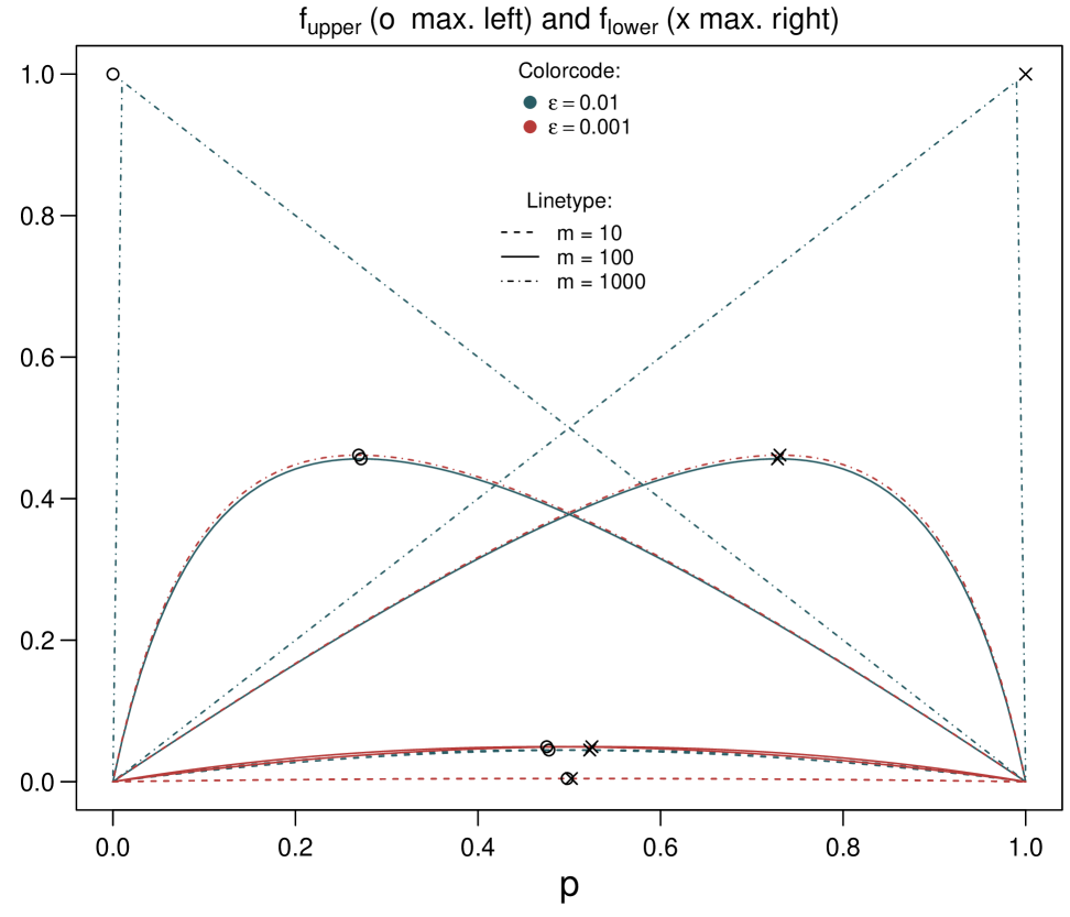
Figure 3: Showing $f_{\text{upper}}$ and $f_{\text{lower}}$ over $[0,1]$ with $d_{2}$ values from Corollary˜8 to use an upper estimate for $p_{\max\Delta}$ by bounding it from above.

∎

Theorem˜7 is crucial in practice, since it lets us compute $D_{CD}(P_{M},P_{M^{\prime}})$ efficiently—without inspecting the full factor graph—and thus has direct practical impact. Since $\frac{\sqrt{e^{d}}-1}{\sqrt{e^{d}}+1}=\tanh\left(\frac{d}{4}\right)\leq 1$ is monotonically strictly increasing in $d$, the results of Theorem˜5 can be substituted into its formula, while the directions of the inequalities are obtained.

Corollary 8.

With previous notations, the change in any probabilistic query in an initial model $M$ and a modified model $M^{\prime}$ obtained by running HACP (Alg.˜2) or $\varepsilon$-ACP is bounded by

$$p_{\max\Delta} \leq\frac{\sqrt{e^{d_{1}}}-1}{\sqrt{e^{d_{1}}}+1}\text{ with }d_{1}=D_{CD}(P_{M},P{{}_{M}^{\prime}})$$

$$\leq\frac{\sqrt{e^{d_{2}}}-1}{\sqrt{e^{d_{2}}}+1}\text{ with }d_{2}=\ln\left(\frac{\big{(}1+\frac{m-1}{m}\varepsilon\big{)}\big{(}1+\varepsilon\big{)}}{1+\frac{1}{m}\varepsilon}\right)^{m}$$

$$\leq\frac{\sqrt{e^{d_{3}}}-1}{\sqrt{e^{d_{3}}}+1}\text{ with }d_{3}=\ln\big{(}1+\varepsilon\big{)}^{2m}$$

$$\leq\frac{\sqrt{e^{d_{4}}}-1}{\sqrt{e^{d_{4}}}+1}\text{ with }d_{4}=\ln\left(\frac{1+\varepsilon}{1-\varepsilon}\right)^{m}.$$

Figure 4: The bound on $p_{\max\Delta}$ depending on the choice of $\varepsilon$ for different amounts of factors $m$.

This implies that for a given $\varepsilon>0$, we can determine the maximum deviation of $p_{\max\Delta}$ (see Fig.˜4). However, it is also essential to consider the reverse perspective to gain insight into the overall diversity and structural complexity of the FG. Therefore, we investigate the following question: What choice of $\varepsilon$ guarantees that our probabilities remain within a specified distance, i.e., $p_{\max\Delta}\leq p_{\Delta}^{*}$? This question is addressed in the subsequent theorem by reversing the preceding inequalities and solving for $\varepsilon$.

Theorem 9.

For any given $p_{\Delta}^{*}\in(0,\frac{1}{2}]$, the output of HACP guarantees for any $\varepsilon\in(0,1)$, which is smaller or equal to

$$\hskip-5.69046pt\varepsilon_{1}=-\frac{1+\tfrac{m-1}{m}-\frac{1}{m}\sqrt[m]{e^{d}}}{2\,\frac{m-1}{m}}+\sqrt{\Bigl{(}-\frac{1+\tfrac{m-1}{m}-\frac{1}{m}\sqrt[m]{e^{d}}}{2\,\frac{m-1}{m}}\Bigr{)}^{2}-\frac{1-\sqrt[m]{e^{d}}}{\tfrac{m-1}{m}}}$$

with $d=\ln\left(\frac{p_{\Delta}^{*}+1}{1-p_{\Delta}^{*}}\right)^{2}$ the bound $p_{\max\Delta}\leq p_{\Delta}^{*}$.

This means that we can bound the maximal deviation $p_{\Delta}^{*}$, which is tight [14], of HACP and $\varepsilon$-ACP, respectively, by calculating $\varepsilon_{1}(p_{\Delta}^{*})$ before we run it.

Proof.

Using Theorem˜7, we get for $d=D_{CD}(P_{M},P{{}_{M}^{\prime}})$:

$$p_{\max\Delta}\leq\frac{\sqrt{e^{d}}-1}{\sqrt{e^{d}}+1}=:p_{\Delta}^{*}$$

$$\Leftrightarrow\ln\left(\frac{p_{\Delta}^{*}+1}{1-p_{\Delta}^{*}}\right)^{2}=d=D_{CD}(P_{M},P{{}_{M}^{\prime}}).$$

Additionally, we use Eq.˜5 from Theorem˜5 and the corresponding version for HACP (Proposition˜6) and solve the inequality for $\varepsilon$, when it reaches equality:

$$\quad\quad\quad\quad\quad~~~d=\ln\left(\frac{\big{(}1+\frac{m-1}{m}\varepsilon\big{)}\big{(}1+\varepsilon\big{)}}{1+\frac{1}{m}\varepsilon}\right)^{m}.~~~~\quad\quad\quad\quad\raisebox{-12.48604pt}{\qed}$$

These bounds are mostly of theoretical nature and the deviations are rarely encountered in reality [14].

Note 2.

Choosing, for instance, a $10$ times larger $\varepsilon$ has pretty much the same effect as choosing $10$ times the number of factors $m$ on the bound on the change in probabilistic queries (cf. Fig.˜3).

Thus, this subsection lays the groundwork for leveraging the supplementary insights from Alg.˜1 to develop a holistic understanding of the structural and computational complexity of the FG. Depending on sensitivity to $\varepsilon$, $p_{\max\Delta}/p_{\Delta}^{*}$, and $m$, one can assess the implications of specific parameter choices on the effect of compressing a given FG, or alternatively, prioritise model fidelity. The HACP algorithm enables such assessments across multiple structural levels.

5 Discussion

Related work.

Lifted inference exploits the indistinguishability of objects in a probabilistic (relational) model, allowing to carry out query answering (i.e., the computation of marginal distributions for randvars given observations for other randvars) more efficiently while maintaining exact answers [16]. First introduced by Poole [17], parametric FGs, which combine relational logic and probabilistic modelling, and lifted variable elimination enable lifted probabilistic inference to speed up query answering by exploiting the indistinguishability of objects. Over the past years, lifted variable elimination has continuously been refined by many researchers to reach its current form [3, 5, 6, 11, 15, 19]. To construct a lifted (i.e., first-order) representation such as a parametric FG, the ACP algorithm [13], which generalises the CompressFactorGraph algorithm [1, 10], is the current state of the art. acp runs a colour passing procedure to detect symmetric subgraphs in a probabilistic graphical model, similar to the Weisfeiler-Leman algorithm [23], which is a well-known algorithm to test for graph isomorphism. The idea is then to group symmetric subgraphs and exploit exponentiation during probabilistic inference. While ACP is able to construct a parametric FG entailing equivalent semantics as a given propositional model, it requires potentials of factors to exactly match before grouping them. In practical applications, however, potentials are often estimates and hence might slightly differ even for indistinguishable objects. To account for small deviations between potentials, the $\varepsilon$-ACP algorithm [14] has been introduced, generalising ACP by introducing a hyperparameter $\varepsilon$ that controls the trade-off between the exactness and the compactness of the resulting lifted representation.

Pre-ordering means pre-analysing.

Our hierarchical algorithm (Alg.˜1) imposes a predetermined nesting structure on the factor graph before any colour passing procedure, enabling application-oriented level selection that is specified a priori. By fixing the levels to consider before invoking Alg.˜2 on the adjusted graph, one can predict the resulting complexity of $\varepsilon$-equivalent group structure and thereby enhance interpretability. In contrast to $\varepsilon$-ACP, which may produce $\varepsilon$-equivalent groupings that lack consistent nesting across runs or parameter settings, our hierarchical approach (HACP) ensures structural coherence and comparability across instances. Moreover, the explicit composition of each level can be monitored to trace the impact of modifications throughout the hierarchy.

Trade-off: Compression versus Accuracy.

Both $\varepsilon$-ACP and HACP inherit the deviation bounds introduced by Luttermann et al. [14], yielding identical sharp bounds and dependency structures for any choice of $\varepsilon$. In practice, the precise grouping composition governs the magnitude and sign of probabilistic deviations for downstream queries: As the hierarchy level (or $\varepsilon$) increases, theoretical bounds grow, yet actual query deviations may fluctuate based on group aggregations. Crucially, our hierarchical bounds facilitate pre-specification of maximal permissible $\varepsilon$ values and corresponding levels. Rather than relying on the generally intractable $D_{CD}$ for approximated models [4], one can derive $p_{\max\Delta}$ for a given $\varepsilon$, or select an admissible level that guarantees both desired compression and sufficient accuracy.

6 Conclusion

We introduce a novel framework for hierarchical lifting and model reconciliation in FGs. By presenting a more practical one-dimensional notion of $\varepsilon$-equivalent factors, we enable the identification of (possibly inexact) symmetries, the number and sizes of $\varepsilon$-equivalent groups and the resulting reduction of computational complexity, thereby allowing for lifted inference. Our theoretical analysis provides a solid foundation for understanding the structural properties of FGs. Crucially, the entire hierarchy is fixed prior to initiating colour passing or inference, ensuring structural consistency and enabling theoretical error bounds. This work provides a foundation for future advances in efficient and interpretable probabilistic inference.

This work was partially funded by the Ministry of Culture and Science of the German State of North Rhine-Westphalia. The research of Malte Luttermann was funded by the BMBF project AnoMed 16KISA057.

Appendix

1 Counterexamples

Proposition 10.

The 1DEED is not a metric.

Proof.

The 1DEED is not a metric, because the $\Delta$-inequality does not hold, which is exemplarily proven by this counterexample:

$$\phi_{1} =\begin{pmatrix}2\\ 0.5\end{pmatrix},\phi_{2}=\begin{pmatrix}1\\ 1\end{pmatrix},\phi_{3}=\begin{pmatrix}1\\ 2\end{pmatrix}$$

with $d_{\infty}(\phi_{1},\phi_{2})+d_{\infty}(\phi_{2},\phi_{3})=1+1<3=d_{\infty}(\phi_{1},\phi_{3})$. ∎

Proposition 11.

The 1DEED lacks the transitivity property.

Proof.

Given a Boolean random variable $Var$, consider three factors $\phi_{1},\phi_{2},\phi_{3}$ defined as follows:

$Var$	$\phi_{1}(Var)$	$\phi_{2}(Var)$	$\phi_{3}(Var)$
true	$0.95$	$1.0$	$1.08$
false	$2.05$	$1.95$	$2.10$

Using the 1DEED with $\varepsilon=0.1$, we end up with $\phi_{1}=_{\varepsilon}\phi_{2}$ and $\phi_{2}=_{\varepsilon}\phi_{3}$, but $\phi_{1}\neq_{\varepsilon}\phi_{3}$:

$$\phi_{1}(\text{true})=0.95<0.972=(1-\varepsilon)1.08=(1-\varepsilon)\phi_{3}(\text{true}).$$

∎

2 Missing Proofs

Theorem 3.

Def. 3 and Def. 4 (main paper) of $\varepsilon$-equivalence for two vectors $\phi_{1},\phi_{2}\in\mathbb{R}_{>0}^{n}$ are equivalent.

Proof.

In mathematical terms, the claim can be summarised as $\phi_{1}=_{\varepsilon}\phi_{2}\Leftrightarrow d_{\infty}(\phi_{1},\phi_{2})\leq\varepsilon$, which we prove for any $\varepsilon>0$:

$$\phi_{1}=_{\varepsilon}\phi_{2}\text{ for two factors }\phi_{1},\phi_{2}\in\mathbb{R}_{>0}^{n}$$

$$\overset{\text{def.}}{\Leftrightarrow}\phi_{1}(k)\in[(1-\varepsilon)\phi_{2}(k),(1+\varepsilon)\phi_{2}(k)]\text{ and }$$

$$\quad~~~\phi_{2}(k)\in[(1-\varepsilon)\phi_{1}(k),(1+\varepsilon)\phi_{1}(k)]\text{ for }k=1,\ldots,n$$

$$\Leftrightarrow\phi_{2}(k)-\phi_{2}(k)\varepsilon\leq\phi_{1}(k)\leq\phi_{2}(k)+\varepsilon\phi_{2}(k)\text{ and }$$

$$\quad~~~\phi_{1}(k)-\phi_{1}(k)\varepsilon\leq\phi_{2}(k)\leq\phi_{1}(k)+\varepsilon\phi_{1}(k)\text{ for }k=1,\ldots,n$$

$$\Leftrightarrow-\phi_{2}(k)\varepsilon\leq\phi_{1}(k)-\phi_{2}(k)\leq\varepsilon\phi_{2}(k)\text{ and }$$

$$\quad~~~-\phi_{1}(k)\varepsilon\leq\phi_{2}(k)-\phi_{1}(k)\leq\varepsilon\phi_{1}(k)\text{ for }k=1,\ldots,n$$

$$\Leftrightarrow|\phi_{1}(k)-\phi_{2}(k)|\leq\varepsilon\phi_{2}(k)\text{ and }$$

$$\quad~~~|\phi_{1}(k)-\phi_{2}(k)|\leq\varepsilon\phi_{1}(k)\text{ for }k=1,\ldots,n$$

$$\Leftrightarrow\frac{|\phi_{1}(k)-\phi_{2}(k)|}{\phi_{2}(k)}\leq\varepsilon\text{ and }$$

$$\quad~~~\frac{|\phi_{1}(k)-\phi_{2}(k)|}{\phi_{1}(k)}\leq\varepsilon\text{ for }k=1,\ldots,n$$

$$\Leftrightarrow\frac{|\phi_{1}(k)-\phi_{2}(k)|}{\min\{\phi_{1}(k),\phi_{2}(k)\}}\leq\varepsilon\text{ for }k=1,\ldots,n$$

$$\Leftrightarrow\max_{k=1,\ldots,n}\left\{\frac{|\phi_{1}(k)-\phi_{2}(k)|}{\min\{\phi_{1}(k),\phi_{2}(k)\}}\right\}\leq\varepsilon$$

$$\overset{\text{def.}}{\Leftrightarrow}d_{\infty}(\phi_{1},\phi_{2})\leq\varepsilon\qed$$

Theorem 7.

The maximal absolute deviation between any initial probability $p=P_{M}(r\mid\boldsymbol{e})$ of $r$ given $\boldsymbol{e}$ in model $M$ and the probability $p^{\prime}=P_{M^{\prime}}(r\mid\boldsymbol{e})$ in the modified model $M^{\prime}$ resulting from running Hierarchical Advanced Colour Passing (HACP, main paper, Alg. 2) or $\varepsilon$-Advanced Colour Passing ($\varepsilon$-ACP) on $M$ can be bounded by

$$p_{\max\Delta}:=\max_{\text{for any }r\mid\boldsymbol{e}}|p-p^{\prime}|\leq\frac{\sqrt{e^{d}}-1}{\sqrt{e^{d}}+1}\text{ with }d=D_{CD}(P_{M},P{{}_{M}^{\prime}}).$$

Proof.

From Chan and Darwiche [1], we already know that

$$\frac{pe^{-d}}{p(e^{-d}-1)+1}\leq p^{\prime}=P_{M^{\prime}}(r\mid\boldsymbol{e})\leq\frac{pe^{d}}{p(e^{d}-1)+1}$$ (8)

holds (see Fig.˜5), where $p=P_{M}(r\mid\boldsymbol{e})$ is the probability of $r$ given $\boldsymbol{e}$ in the original model $M$ and $d=D_{CD}(P_{M},P{{}_{M}^{\prime}})$ is the value of the distance measure introduced by Chan and Darwiche between $P_{M}$ and $P{{}_{M}^{\prime}}$. Hence, for any $r$ given $\boldsymbol{e}$, in the worst case, we get

$$|p-p^{\prime}|=\begin{cases}p^{\prime}-p&\text{for }p\leq p^{\prime}\\ p-p^{\prime}&\text{for }p^{\prime}<p\end{cases}=\begin{cases}\frac{pe^{d}}{p(e^{d}-1)+1}-p&\text{for }p\leq p^{\prime}\\ p-\frac{pe^{-d}}{p(e^{-d}-1)+1}&\text{for }p^{\prime}<p.\end{cases}$$

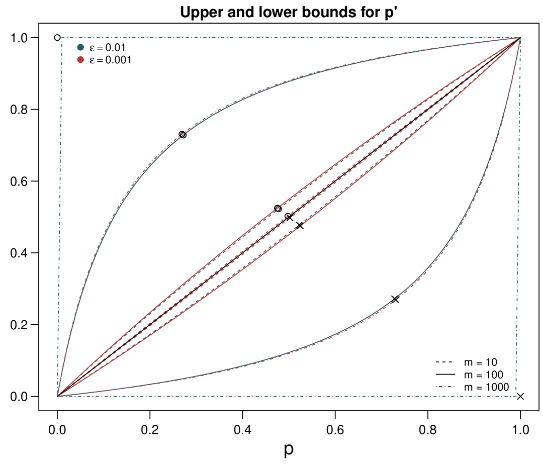
Figure 5: Bounds of Eq.˜8 in comparison to $p$ for different $d$ values depending on $m$ and $\varepsilon$ (Eq. (5) of the main paper). Circles/ crosses are the maximum distances from those bounds to the function $p$. Distances to function $f(p)=p$ are later also referred as $f=f_{\text{upper}}$ for $p\in[0,\frac{1}{2}]$ and $f=f_{\text{lower}}$ for $p\in(\frac{1}{2},1]$.

Becoming independent of $p^{\prime}$ guarantees one maximal bound for all possible queries and can be achieved using the maximum of both cases in $[0,1]$ as an upper bound for $p_{\max\Delta}$, which is given by the following function $f_{\max\Delta}(p)$:

$$f_{\max\Delta}(p):= \max(f_{\text{upper}}(p),f_{\text{lower}}(p))\text{ for }p\in[0,1]$$

$$\text{with }f_{\text{upper}}(p):= \frac{pe^{d}}{p(e^{d}-1)+1}-p=\frac{p(1-p)(e^{d}-1)}{p(e^{d}-1)+1}$$

$$\text{and }f_{\text{lower}}(p):= p-\frac{pe^{-d}}{p(e^{-d}-1)+1}=\frac{p(1-p)(1-e^{-d})}{p(e^{-d}-1)+1}.$$

Figure 6: Showing the $f_{\text{upper}}$ and $f_{\text{lower}}$ functions over $[0,1]$ with $d_{2}$ values from Corollary 8 to use an upper estimate for $p_{\max\Delta}$ by bounding it from above.

It is easy to see that $f_{\max\Delta}$ is a symmetric function around $p=0.5$ (see Fig.˜6), because $f_{\text{upper}}(p)=f_{\text{lower}}(1-p)$ holds:

$$f_{\text{lower}}(1-p) =\frac{(1-p)p(1-e^{-d})}{(1-p)(e^{-d}-1)+1}$$

$$=\frac{(1-p)p(e^{d}-1)e^{-d}}{(1-p)(e^{-d}-1)+1}$$

$$=\frac{(1-p)p(e^{d}-1)}{((1-p)(e^{-d}-1)+1)e^{d}}$$

$$=\frac{p(1-p)(e^{d}-1)}{(1-p)(1-e^{d})+e^{d}}$$

$$=\frac{p(1-p)(e^{d}-1)}{1-p+pe^{d}}$$

$$=\frac{p(1-p)(e^{d}-1)}{p(e^{d}-1)+1}$$

$$=f_{\text{upper}}(p)$$

Now, the choice for $p^{\prime}$ to get the maximum of both functions is $p=0.5$, while $f_{\text{upper}}(p)$ decreases for $p>0.5$ and $f_{\text{lower}}(p)$ increases for $p<0.5$ for $d\geq 0$. Therefore, we get

$$f_{\max\Delta}(p):=\begin{cases}f_{\text{upper}}(p)&\text{for }0\leq p\leq 0.5\\ f_{\text{lower}}(p)&\text{for }0.5<p\leq 1\end{cases}$$ (9)

This means that our search for the maximum deviation leads us to calculate the derivatives after $p$

$$f_{\text{upper}}^{\prime}(p) =-\frac{(e^{d}-1)(p^{2}(e^{d}-1)+2p-1)}{(p(e^{-d}-1)+1)^{2}},$$

$$f_{\text{upper}}^{\prime\prime}(p) =\frac{-2e^{d}(e^{d}-1)}{(p(e^{d}-1)+1)^{3}},$$

$$f_{\text{lower}}^{\prime}(p) =\frac{(1-e^{-d})(p^{2}(1-e^{-d})-2p+1)}{(p(e^{-d}-1)+1)^{2}},$$

$$f_{\text{lower}}^{\prime\prime}(p) =\frac{-2e^{d}(e^{d}-1)}{(p+e^{d}(1-p))^{3}},$$

and to consider initially the first-order conditions. For this purpose, we first obtain

$$f_{\text{upper}}^{\prime}(p) =0$$

$$\Leftrightarrow p^{2}(e^{d}-1)+2p-1=0$$

$$\Leftrightarrow p_{\text{upper }1/2}=-\frac{1}{e^{d}-1}\pm\sqrt{\left(\frac{-1}{e^{d}-1}\right)^{2}+\frac{1}{e^{d}-1}}$$

$$\Leftrightarrow p_{\text{upper }1/2}=-\frac{1}{e^{d}-1}\pm\frac{\sqrt{e^{d}}}{e^{d}-1}=\frac{-1\pm\sqrt{e^{d}}}{e^{d}-1}.$$

As $p_{\text{upper }2}$ is smaller than zero, the potential maximum in $[0,1]$ is at

$$p_{1}=p_{\text{upper }1}=\frac{\sqrt{e^{d}}-1}{e^{d}-1}=\frac{1}{\sqrt{e^{d}}+1}.$$

Analogously, we find a potential maximum for $f_{\text{lower}}^{\prime}$:

$$f_{\text{lower}}^{\prime}(p) =0$$

$$\Leftrightarrow p^{2}(1-e^{-d})-2p+1=0$$

$$\Leftrightarrow p_{\text{lower }1/2}=\frac{1}{1-e^{-d}}\pm\sqrt{\left(\frac{1}{1-e^{-d}}\right)^{2}-\frac{1}{1-e^{-d}}}$$

$$\Leftrightarrow p_{\text{lower }1/2}=\frac{1}{1-e^{-d}}\pm\frac{\sqrt{e^{-d}}}{1-e^{-d}}=\frac{1\pm\sqrt{e^{-d}}}{1-e^{-d}}$$

As $p_{\text{lower }1}$ is larger than one, the possible maximum in $[0,1]$ is at

$$p_{2}=p_{\text{lower }2}=\frac{1-\sqrt{e^{-d}}}{1-e^{-d}}=\frac{1}{\sqrt{e^{-d}}+1}=\frac{\sqrt{e^{d}}}{\sqrt{e^{d}}+1}$$

and the second-order conditions can also be easily checked:
Since $e^{d}-1>0$ and $1-p>0$, we get $f_{\text{upper}}^{\prime\prime}(p_{1})<0$ and $f_{\text{lower}}^{\prime\prime}(p_{2})<0$ and can conclude that $p_{1}$ is a local maximum of $f_{\text{upper}}$ and $p_{2}$ is a local maximum of $f_{\text{lower}}$. The boundary values $0$ and $1$ are no possible points for a global maximum, because both functions $f_{\text{upper}}$ and $f_{\text{lower}}$ take on the value $0$ there. Therefore, the only possible extreme point for the global maximum for $f_{\text{upper}}$ is $p_{1}=\frac{1}{\sqrt{e^{d}}+1}$ and $f_{\text{lower}}$ is $p_{2}=\frac{\sqrt{e^{d}}}{\sqrt{e^{d}}+1}$. Note that $p_{1}$ and $p_{2}$ are symmetrically distanced to $p=1/2$.
Both reach exactly the same maximal deviation:

$$f_{\text{upper}}(p_{1}) =\frac{\frac{1}{\sqrt{e^{d}}+1}(1-\frac{1}{\sqrt{e^{d}}+1})(e^{d}-1)}{\frac{1}{\sqrt{e^{d}}+1}(e^{d}-1)+1}$$

$$=\frac{\frac{1}{\sqrt{e^{d}}+1}\cdot\frac{\sqrt{e^{d}}}{\sqrt{e^{d}}+1}\cdot(\sqrt{e^{d}}+1)\cdot(\sqrt{e^{d}}-1)}{\frac{e^{d}-1+\sqrt{e^{d}}+1}{\sqrt{e^{d}}+1}}$$

$$=\frac{\sqrt{e^{d}}(\sqrt{e^{d}}-1)}{e^{d}+\sqrt{e^{d}}}=\frac{\sqrt{e^{d}}-1}{\sqrt{e^{d}}+1}$$

and the same holds for

$$f_{\text{lower}}(p_{2}) =\frac{\frac{\sqrt{e^{d}}}{\sqrt{e^{d}}+1}(1-\frac{\sqrt{e^{d}}}{\sqrt{e^{d}}+1})(1-e^{-d})}{\frac{\sqrt{e^{d}}}{\sqrt{e^{d}}+1}(e^{-d}-1)+1}$$

$$=\frac{\frac{\sqrt{e^{d}}}{\sqrt{e^{d}}+1}\cdot\frac{1}{\sqrt{e^{d}}+1}\cdot(1-e^{-d})}{\frac{\sqrt{e^{d}}}{\sqrt{e^{d}}+1}\cdot(\sqrt{e^{-d}}-\sqrt{e^{d}}+\sqrt{e^{d}}+1)}$$

$$=\frac{\sqrt{e^{d}}(1-\sqrt{e^{-d}})(1+\sqrt{e^{-d}})}{(\sqrt{e^{-d}}+1)(\sqrt{e^{d}}+1)}$$

$$=\frac{\sqrt{e^{d}}-1}{\sqrt{e^{d}}+1}.$$

This means:

$$p_{\max\Delta} =\max_{\text{for any }r\mid\boldsymbol{e}}|p-p^{\prime}|$$

$$\leq f_{\text{upper}}(p_{1})=f_{\text{lower}}(p_{2})$$

$$=\frac{\sqrt{e^{d}}-1}{\sqrt{e^{d}}+1}\qed$$

Theorem 9.

For any given $p_{\Delta}^{*}\in(0,\frac{1}{2}]$, the output of HACP guarantees for any $\varepsilon\in(0,1)$, which is smaller or equal to

$$\varepsilon_{1}= -\frac{1+\frac{m-1}{m}-\frac{1}{m}\sqrt[m]{e^{d}}}{2\frac{m-1}{m}}$$

$$+\sqrt{\left(-\frac{1+\frac{m-1}{m}-\frac{1}{m}\sqrt[m]{e^{d}}}{2\frac{m-1}{m}}\right)^{2}-\frac{1-\sqrt[m]{e^{d}}}{\frac{m-1}{m}}}$$

with

$$d=\ln\left(\frac{p_{\Delta}^{*}+1}{1-p_{\Delta}^{*}}\right)^{2}$$

the bound $p_{\max\Delta}\leq p_{\Delta}^{*}$.

This means that we can bound the maximal deviation $p_{\Delta}^{*}$ of HACP and $\varepsilon$-ACP, respectively, by calculating $\varepsilon_{1}(p_{\Delta}^{*})$ before we run it. In [2], it is shown that the bound is tight.

Proof.

Using Theorem˜7, we get for $d=D_{CD}(P_{M},P{{}_{M}^{\prime}})$:

$$p_{\max\Delta}\leq\frac{\sqrt{e^{d}}-1}{\sqrt{e^{d}}+1}=:p_{\Delta}^{*}$$

$$\Leftrightarrow p_{\Delta}^{*}\left(\sqrt{e^{d}}+1\right)=\sqrt{e^{d}}-1$$

$$\Leftrightarrow p_{\Delta}^{*}+1=(1-p_{\Delta}^{*})\sqrt{e^{d}}$$

$$\Leftrightarrow\frac{p_{\Delta}^{*}+1}{1-p_{\Delta}^{*}}=\sqrt{e^{d}}$$

$$\Leftrightarrow\ln\left(\frac{p_{\Delta}^{*}+1}{1-p_{\Delta}^{*}}\right)^{2}=d=D_{CD}(P_{M},P{{}_{M}^{\prime}}).$$

Additionally, we know from Theorem 5 and the corresponding version for HACP (Proposition 6) that

$$D_{CD}(P_{M},P{{}_{M}^{\prime}})\leq\ln\left(\frac{\big{(}1+\frac{m-1}{m}\varepsilon\big{)}\big{(}1+\varepsilon\big{)}}{1+\frac{1}{m}\varepsilon}\right)^{m}.$$ (10)

Thus, the question we now answer is for which $\varepsilon$ this inequality reaches equality:

$$d=\ln\left(\frac{\big{(}1+\frac{m-1}{m}\varepsilon\big{)}\big{(}1+\varepsilon\big{)}}{1+\frac{1}{m}\varepsilon}\right)^{m}$$

$$\Leftrightarrow ~\sqrt[m]{e^{d}}=\frac{\big{(}1+\frac{m-1}{m}\varepsilon\big{)}\big{(}1+\varepsilon\big{)}}{1+\frac{1}{m}\varepsilon}$$

$$\Leftrightarrow ~\big{(}1+\frac{1}{m}\varepsilon\big{)}\sqrt[m]{e^{d}}=\big{(}1+\frac{m-1}{m}\varepsilon\big{)}\big{(}1+\varepsilon\big{)}$$

$$\Leftrightarrow ~0=\frac{m-1}{m}\varepsilon^{2}+\big{(}1+\frac{m-1}{m}-\frac{1}{m}\sqrt[m]{e^{d}}\big{)}\varepsilon+1-\sqrt[m]{e^{d}},$$

which can be solved for $\varepsilon$ with $q_{1}=\frac{1+\frac{m-1}{m}-\frac{1}{m}\sqrt[m]{e^{d}}}{\frac{m-1}{m}}$ and $q_{2}=\frac{1-\sqrt[m]{e^{d}}}{\frac{m-1}{m}}$, resulting in

$$\varepsilon_{1/2}=-\frac{q_{1}}{2}\pm\sqrt{\big{(}\frac{q_{1}}{2}\big{)}^{2}-q_{2}}.$$

Since $q_{1}\geq 0\Leftrightarrow\frac{m-1}{m}\geq p^{*}_{\Delta}$, the minus option $\varepsilon_{2}$ is smaller than $0$ and knowing that $m\geq 2$ already guarantees the result of Theorem˜9, for all cases which make sense to apply (better than guessing $\geq 0.5$), the only reasonable solution is $\varepsilon_{1}$. ∎

Figure 7: The maximal choice of $\varepsilon$ depending on the maximal deviation $p_{\Delta}^{*}$ for different amount of factors $m$ to guarantee $p_{\max\Delta}\leq p_{\Delta}^{*}$ as proven in Theorem˜9.

3 The Basic Idea of Lifting

To illustrate the idea behind lifting, consider the following example.

Example 4.

Take a look at the FG illustrated in Fig.˜8 and assume we want to answer the query $P(B=\text{true})$. We obtain

$$P(B=\text{true}) =\sum_{a\in\text{range}(A)}\sum_{c\in\text{range}(C)}P(A=a,B=\text{true},C=c)$$

$$=\frac{1}{Z}\sum_{a\in\text{range}(A)}\sum_{c\in\text{range}(C)}\phi_{1}(a,\text{true})\cdot\phi_{2}(c,\text{true})$$

$$=\frac{1}{Z}\Big{(}\varphi_{1}\varphi_{1}+\varphi_{1}\varphi_{3}+\varphi_{3}\varphi_{1}+\varphi_{3}\varphi_{3}\Big{)}.$$

Since $\phi_{1}(A,B)$ and $\phi_{2}(C,B)$ are equivalent (in particular, it holds that $\phi_{1}(a,\text{true})=\phi_{2}(c,\text{true})$ for all assignments where $a=c$), we can exploit this property to simplify the computation and get

$$P(B=\text{true}) =\frac{1}{Z}\sum_{a\in\text{range}(A)}\sum_{c\in\text{range}(C)}\phi_{1}(a,\text{true})\cdot\phi_{2}(c,\text{true})$$

$$=\frac{1}{Z}\sum_{a\in\text{range}(A)}\phi_{1}(a,\text{true})\sum_{c\in\text{range}(C)}\phi_{2}(c,\text{true})$$

$$=\frac{1}{Z}\Bigg{(}\sum_{a\in\text{range}(A)}\phi_{1}(a,\text{true})\Bigg{)}^{2}$$

$$=\frac{1}{Z}\Bigg{(}\sum_{c\in\text{range}(C)}\phi_{2}(c,\text{true})\Bigg{)}^{2}$$

$$=\frac{1}{Z}\Big{(}\varphi_{1}+\varphi_{3}\Big{)}^{2}.$$

This example illustrates the idea of using a representative of indistinguishable objects for computations (here, either $A$ or $C$ can be chosen as a representative for the group consisting of $A$ and $C$).

Figure 8: An exemplary FG encoding a full joint probability distribution over three random variables $A$, $B$, and $C$.

The idea of exploiting exponentiation can be generalised to groups consisting of $k$ indistinguishable objects to significantly reduce the computational effort for query answering. To be able to exploit exponentiation during probabilistic inference, we need to ensure that the potential tables of factors within the same group are identical. Indistinguishable objects frequently occur in many real world domains. For example, in an epidemic domain, each person impacts the probability of having an epidemic equally. That is, the probability of an epidemic depends on the number of sick people in the universe but is independent of which specific individual people are sick.

4 Group Sizes of an Hierarchical Ordering

Table˜2 shows for each level of the hierarchy in Fig. 2 of the main paper how many $\varepsilon$-equivalent groups of which size exist. Thus, it illustrates the increasing compression that is possible with increasing $\varepsilon$ values.

Level	Number of total groups	Group Size (Frequency)
0	10	1 (10),
1	9	2 (1), 1 (8)
2	8	2 (2), 1 (6)
3	7	2 (3), 1 (4)
4	6	4 (1), 2 (1), 1 (4)
5	5	4 (1), 3 (1), 1 (3)
6	4	4 (1) , 3 (1), 2 (1), 1 (1)
7	3	7 (1), 2 (1), 1 (1)
8	2	7 (1), 3 (1)
9	1	10 (1)

Table 2: Implicit group sizes for each level for given structure and pre-ordered FG for Ex. 3 from the main paper.

References

- Ahmadi et al. [2013] B. Ahmadi, K. Kersting, M. Mladenov, and S. Natarajan. Exploiting Symmetries for Scaling Loopy Belief Propagation and Relational Training. Machine Learning, 92(1):91–132, 2013.
- Braun and Möller [2016] T. Braun and R. Möller. Lifted Junction Tree Algorithm. In Proceedings of the Thirty-Ninth German Conference on Artificial Intelligence (KI-2016), pages 30–42. Springer, 2016.
- Braun and Möller [2018] T. Braun and R. Möller. Parameterised Queries and Lifted Query Answering. In Proceedings of the Twenty-Seventh International Joint Conference on Artificial Intelligence (IJCAI-2018), pages 4980–4986. IJCAI Organization, 2018.
- Chan and Darwiche [2005] H. Chan and A. Darwiche. A Distance Measure for Bounding Probabilistic Belief Change. International Journal of Approximate Reasoning, 38:149–174, 2005.
- De Salvo Braz et al. [2005] R. De Salvo Braz, E. Amir, and D. Roth. Lifted First-Order Probabilistic Inference. In Proceedings of the Nineteenth International Joint Conference on Artificial Intelligence (IJCAI-2005), pages 1319–1325. Morgan Kaufmann Publishers Inc., 2005.
- De Salvo Braz et al. [2006] R. De Salvo Braz, E. Amir, and D. Roth. MPE and Partial Inversion in Lifted Probabilistic Variable Elimination. In Proceedings of the Twenty-First National Conference on Artificial Intelligence (AAAI-2006), pages 1123–1130. AAAI Press, 2006.
- Frey et al. [1997] B. J. Frey, F. R. Kschischang, H.-A. Loeliger, and N. Wiberg. Factor Graphs and Algorithms. In Proceedings of the Thirty-Fifth Annual Allerton Conference on Communication, Control, and Computing, pages 666–680. Allerton House, 1997.
- Gogate and Domingos [2011] V. Gogate and P. Domingos. Probabilistic Theorem Proving. In Proceedings of the Twenty-Seventh Conference on Uncertainty in Artificial Intelligence (UAI-2011), pages 256–265. AUAI Press, 2011.
- Hartwig et al. [2024] M. Hartwig, R. Möller, and T. Braun. An Extended View on Lifting Gaussian Bayesian Networks. Artificial Intelligence, 330:104082, 2024.
- Kersting et al. [2009] K. Kersting, B. Ahmadi, and S. Natarajan. Counting Belief Propagation. In Proceedings of the Twenty-Fifth Conference on Uncertainty in Artificial Intelligence (UAI-2009), pages 277–284. AUAI Press, 2009.
- Kisyński and Poole [2009] J. Kisyński and D. Poole. Constraint Processing in Lifted Probabilistic Inference. In Proceedings of the Twenty-Fifth Conference on Uncertainty in Artificial Intelligence (UAI-2009), pages 293–302. AUAI Press, 2009.
- Kschischang et al. [2001] F. R. Kschischang, B. J. Frey, and H.-A. Loeliger. Factor Graphs and the Sum-Product Algorithm. IEEE Transactions on Information Theory, 47:498–519, 2001.
- Luttermann et al. [2024] M. Luttermann, T. Braun, R. Möller, and M. Gehrke. Colour Passing Revisited: Lifted Model Construction with Commutative Factors. In Proceedings of the Thirty-Eighth AAAI Conference on Artificial Intelligence (AAAI-2024), pages 20500–20507. AAAI Press, 2024.
- Luttermann et al. [2025] M. Luttermann, J. Speller, M. Gehrke, T. Braun, R. Möller, and M. Hartwig. Approximate Lifted Model Construction. In Proceedings of the Thirty-Fourth International Joint Conference on Artificial Intelligence (IJCAI-2025), 2025. https://arxiv.org/abs/2504.20784.
- Milch et al. [2008] B. Milch, L. S. Zettlemoyer, K. Kersting, M. Haimes, and L. P. Kaelbling. Lifted Probabilistic Inference with Counting Formulas. In Proceedings of the Twenty-Third AAAI Conference on Artificial Intelligence (AAAI-2008), pages 1062–1068. AAAI Press, 2008.
- Niepert and Van den Broeck [2014] M. Niepert and G. Van den Broeck. Tractability through Exchangeability: A New Perspective on Efficient Probabilistic Inference. In Proceedings of the Twenty-Eighth AAAI Conference on Artificial Intelligence (AAAI-2014), pages 2467–2475. AAAI Press, 2014.
- Poole [2003] D. Poole. First-order Probabilistic Inference. In Proceedings of the Eighteenth International Joint Conference on Artificial Intelligence (IJCAI-2003), pages 985–991. IJCAI Organization, 2003.
- Richardson and Domingos [2006] M. Richardson and P. Domingos. Markov Logic Networks. Machine Learning, 62(1–2):107–136, 2006.
- Taghipour et al. [2013] N. Taghipour, D. Fierens, J. Davis, and H. Blockeel. Lifted Variable Elimination: Decoupling the Operators from the Constraint Language. Journal of Artificial Intelligence Research, 47(1):393–439, 2013.
- Van den Broeck [2013] G. Van den Broeck. Lifted Inference and Learning in Statistical Relational Models. PhD thesis, KU Leuven, 2013.
- Van den Broeck and Davis [2012] G. Van den Broeck and J. Davis. Conditioning in First-Order Knowledge Compilation and Lifted Probabilistic Inference. In Proceedings of the Twenty-Sixth AAAI Conference on Artificial Intelligence (AAAI-2012), pages 1961–1967. AAAI Press, 2012.
- Van den Broeck et al. [2011] G. Van den Broeck, N. Taghipour, W. Meert, J. Davis, and L. De Raedt. Lifted Probabilistic Inference by First-order Knowledge Compilation. In Proceedings of the Twenty-Second International Joint Conference on Artificial Intelligence (IJCAI-2011), pages 2178–2185. IJCAI Organization, 2011.
- Weisfeiler and Leman [1968] B. Weisfeiler and A. A. Leman. The Reduction of a Graph to Canonical Form and the Algebra which Appears Therein. NTI, Series, 2:12–16, 1968. English translation by Grigory Ryabov available at https://www.iti.zcu.cz/wl2018/pdf/wl_paper_translation.pdf.

References

- [1] H. Chan and A. Darwiche. A distance measure for bounding probabilistic belief change. International Journal of Approximate Reasoning, 38:149–174, 2005.
- [2] M. Luttermann, J. Speller, M. Gehrke, T. Braun, R. Möller, and M. Hartwig. Approximate lifted model construction. In Proceedings of the Thirty-Fourth International Joint Conference on Artificial Intelligence (IJCAI-2025), 2025. https://arxiv.org/abs/2504.20784.