Wireless Communication for Low-Altitude Economy with UAV Swarm Enabled
Two-Level Movable Antenna System

Abstract

Unmanned aerial vehicle (UAV) is regarded as a key enabling platform for low-altitude economy, due to its advantages such as three-dimensional (3D) maneuverability, flexible deployment, and line-of-sight (LoS) air-to-air/ground communication links. In particular, the intrinsic high mobility renders UAV especially suitable for operating as a movable antenna (MA) from the sky. In this paper, by exploiting the flexible mobility of UAV swarm and antenna position adjustment of MA, we propose a novel UAV swarm enabled two-level MA system, where UAVs not only individually deploy a local MA array, but also form a larger-scale MA system with their individual MA arrays via swarm coordination. We formulate a general optimization problem to maximize the minimum achievable rate over all ground user equipments (UEs), by jointly optimizing the 3D UAV swarm placement positions, their individual MAs’ positions (or local positions), and receive beamforming for different UEs. To gain useful insights, we first consider the special case where each UAV has only one antenna, under different scenarios of one single UE, two UEs, and arbitrary number of UEs. In particular, for the two-UE case, we derive the optimal UAV swarm placement positions in closed-form that achieves inter-UE interference (IUI)-free communication, where the UAV swarm forms a uniform sparse array (USA) satisfying collision avoidance constraint. While for the general case with arbitrary number of UEs, we propose an efficient alternating optimization algorithm to solve the formulated non-convex optimization problem. Then, we extend the results to the case where each UAV is equipped with multiple antennas. It is shown that an architecture resembling a modular array can achieve the IUI-free communication in the two-UE case. Numerical results verify that the proposed low-altitude UAV swarm enabled MA system significantly outperforms various benchmark schemes, thanks to the exploitation of two-level mobility to create more favorable channel conditions for multi-UE communications.

I Introduction

Low-altitude economy has emerged as a new integrated economic form, involving assorted low-altitude activities within sub-1,000-meter airspace domains [1, 2]. By leveraging manned/unmanned aerial vehicles (UAVs), and electric vertical take-off and landing (eVTOL) aircrafts, low-altitude economic ecosystems begin to flourish, which encompass a wide range of applications like logistics and delivery, agricultural plant protection, cultural tourism, environmental monitoring, and so on. In particular, benefiting from the advantages such as three-dimensional (3D) maneuverability, flexible deployment, and line-of-sight (LoS) air-to-air/ground communication links, UAV is regarded as an indispensable part of the low-altitude economy, which has driven various applications in wireless communication and sensing [3, 4, 5]. Specifically, from the perspective of wireless communication, there exist two paradigms, i.e., UAV-assisted wireless communication and cellular-connected UAV communication [6]. For example, UAV equipped with base station (BS) or relay can be deployed on demand to assist in the conventional cellular wireless networks, so as to satisfy the ubiquitous connectivity required by the future sixth-generation (6G) wireless network. Extensive research efforts have been devoted to this direction, including UAV channel and energy consumption modeling, performance analysis, and placement/trajectory design [3, 4]. On the other hand, the role of UAV can be shifted from the aerial BS/relay to aerial user equipments (UEs), thus enabling a new paradigm where both the ground and aerial UEs coexist in future wireless networks [6, 7, 3]. Moreover, as integrated sensing and communication (ISAC) has been identified as one of the six major usage scenarios for 6G [8], research on ISAC with UAV has gained a surge of interest recently [9, 10, 11]. Similarly, UAV can act as an aerial anchor for providing the ISAC service from the sky, or an aerial target to be sensed [5].

However, UAVs are subjected to various practical constraints in terms of size, weight, dynamics, and power, rendering a single UAV challenging to execute sophisticated communication or sensing missions [3, 12, 13, 14, 15]. To tackle this issue, UAV swarm, i.e., a group of coordinated UAVs, can cooperatively accomplish sophisticated tasks, e.g., large-scale data collection and environment monitoring. Compared to single UAV, UAV swarm is able to significantly improve the overall payload capability and expand the communication and sensing coverage area. Moreover, the cooperative mechanism helps to reduce the task completion time and offers an enhanced robustness against anomalies or failures than single UAV, since the task of any malfunctioning UAV can be transferred to its neighboring functioning UAVs [16]. Given the above promising advantages, extensive research endeavours have been devoted to UAV swarm assisted communication and sensing. For example, in [17], an efficient channel estimation and self-positioning approach was proposed for UAV swarm communication with unknown displacements among UAVs. The authors in [18] proposed a 3D irregular terrain area coverage scheme with UAV swarm, and the results show that the proposed scheme can cover the area with little redundancy. Besides UAV swarm assisted communication, recent research works have studied the integration of ISAC with UAV swarm, since the LoS-dominating channel is particularly favorable for sensing [5]. Research on UAV swarm ISAC involves various performance metrics, including signal-to-interference-plus-noise ratio (SINR) and achievable rate for communication [2, 11], radar mutual information [19] and Cramér-Rao lower bound (CRLB) for sensing [10, 11, 20]. Despite the promising advantages, UAV swarm also involves several issues, such as the latency caused by information exchange among UAVs, complex collision avoidance planning, and high-precision localization and sensing for UAV swarm regulation [21, 12]. In particular, to tackle the challenge of accurately localizing and sensing the densely located swarm UAVs, a super-resolution communication and sensing method was proposed for UAV swarm in [21].

It is worth mentioning that the inherent flexible mobility of UAV renders it particularly suitable for operating as a movable antenna (MA) [22, 23, 24, 25, 26, 27, 28, 29, 30, 31] or fluid antenna system (FAS) [32, 33] from the sky. For example, each UAV may be equipped with a single or multiple antennas, and a flexible antenna array architecture can be enabled via adjusting the UAV swarm topology. In contrast to conventional fixed-position antenna (FPA) where inter-antenna spacing is usually fixed as half wavelength, MA dynamically adjusts the antenna position via mechanical and/or electrical control, so as to pursue a favorable channel condition and circumvent the deep fading scenario [22, 32]. This thus achieves performance improvement with optimized antenna positions, which may be a complement to extremely large-scale multiple-input multiple-output (MIMO) technique whereby the spectral efficiency and spatial resolution are significantly enhanced via the orders-of-magnitude scaling of antennas [34, 35]. Subsequently, antenna mobility is extended to a more general concept, where both the antenna position and rotation can be flexibly adjusted, i.e., six-dimensional movable antenna (6DMA) [28, 29, 30, 31]. Driven by such new design degrees of freedom (DoFs), a large body of literature focuses on this technology and demonstrates its performance gain in communication outage probability, spectral efficiency and network capacity, as well as sensing accuracy (see [25, 33, 31] and references therein). Besides active MA, the authors in [36] further proposed a new flexible passive reflector architecture, enabling the flexible beamforming direction adjustment via reflector placement and rotation angle optimization.

Note that compared to MAs, UAVs possess even more flexible and wider-range movement, and thus an interesting new idea is to utilize UAV swarm to form MA array. Moreover, different from existing research on MA that only optimizes antenna positions, UAV swarm enabled MA can fully unlock its mobility advantage, where the array geometry is able to be dynamically reconfigured via trajectory optimization, thus yielding a varying array geometry. Preliminary efforts have been devoted to the single UAV-mounted MA [37, 38, 39, 40], and single UAV-mounted passive 6DMA [41], i.e., by carrying an intelligent reflecting surface (IRS) on a UAV [42]. Nevertheless, these works neither take into account the UAV swarm scenario, nor explore the capability of MA system enabled by UAV swarm.

In this paper, motivated by the inherent mobility of UAV swarm and antenna position adjustment of MA, we propose a novel UAV swarm enabled two-level MA system. Specifically, by individually deploying a local MA array on each UAV, all the spatially distributed UAVs cooperatively construct a larger-scale MA system according to their topology. Compared to existing MA systems, UAV swarm enabled MA system involves the dual-scale antenna spatial movement, i.e., the small-scale antenna movement within each local MA array, e.g., at wavelength level, and the large-scale UAV movement, so as to better harness the spatial variations of wireless channels in different scales. By considering low-altitude UAV swarm enabled uplink multi-UE communication, we aim to maximize the minimum achievable rate over all ground UEs. The main contributions of this paper are summarized as follows.

• First, we propose a novel low-altitude UAV swarm enabled two-level MA system, where each UE channel depends on both UAV swarm placement positions and their mounted MA array positions. Subject to the collision avoidance constraint for UAVs [3], as well as mutual coupling avoidance constraint for UAV-mounted MA array, we formulate an optimization problem to maximize the minimum achievable rate over all ground UEs, by jointly optimizing the 3D UAV swarm placement positions, their individual MAs’ positions, and receive beamforming for all UEs.

• Second, to gain useful insights, we consider the special case of single-antenna UAV. It is shown that for the single UE communication, the resulting signal-to-noise ratio (SNR) after applying the optimal maximal-ratio combining (MRC) beamforming only depends on the number of UAVs, irrespective of their array geometry. Then, for the two-UE communication, we derive the optimal UAV swarm placement positions that achieves the maximum communication rate without suffering any inter-UE interference (IUI). The result shows that under the collision avoidance constraint, UAV swarm forms a uniform sparse array (USA) [43] for the IUI-free communication. Moreover, for arbitrary number of UEs, we propose an efficient alternating optimization algorithm to solve the highly non-convex problem, where the optimal receive beamforming is derived in closed-form for given UAV swarm placement positions, and for given receive beamforming, the UAV swarm placement optimization problem can be solved via the successive convex approximation (SCA) technique [3].

• Last, we consider the general case of multi-antenna UAV, where each antenna can move independently within the specified region at its mounted UAV. For the single and two-UE communications, similar results can be obtained as the scenario of single-antenna UAV. In particular, we also consider the special case where all the UAVs adopt the USA [44], the IUI-free communication can be achieved in the two-UE case via joint UAV placement positions and sparsity level adjustment, and the UAV swarm forms an architecture resembling a modular array [45]. Next, the alternating optimization method is applied to solve the problem with arbitrary number of UEs. Numerical results are presented to validate the superior performance of the proposed UAV swarm enabled MA system over various benchmarks, thanks to the two-level mobility to create more favorable channel conditions.

The remainder of the paper is organized as follows. Section II presents the system model of a low-altitude UAV swarm enabled MA system and formulates the problem to maximize the minimum achievable rate among UEs. Section III considers the special case of single-antenna UAV, and the result is extended to the general case of multi-antenna UAV in Section IV. Section V presents the numerical results to validate the performance of UAV swarm enabled MA systems. Finally, we conclude the paper in Section VI.

Notations: Scalars are denoted by italic letters. Vectors and matrices are denoted by bold-face lower- and upper-case letters, respectively. The spaces of $M\times N$ complex-valued matrices are denoted as ${{\mathbb{C}}^{M\times N}}$. For a vector ${\bf{x}}$, $\left\|{\bf{x}}\right\|$ denotes its Euclidean norm. For an arbitrary-size matrix ${\bf A}$, its complex conjugate, transpose, and Hermitian transpose are denoted by ${\bf A}^{*}$, ${\bf A}^{T}$, ${\bf A}^{H}$, respectively. The spectral norm and Frobenius norm of ${\bf A}$ are denoted as ${\left\|{\bf{A}}\right\|_{\lx@text@underscore}2}$ and ${\left\|{\bf{A}}\right\|_{\lx@text@underscore}F}$, respectively. The distribution of a circularly symmetric complex Gaussian random vector with mean $\bf{x}$ and covariance matrix $\bf{\Sigma}$ is denoted as ${\cal CN}\left({\bf{x},\bf{{\Sigma}}}\right)$, and $\sim$ stands for “distributed as”. For a complex-valued number $x$, ${\mathop{\rm Re}\nolimits}\left\{x\right\}$ represents its real part. $\bmod\left({a,b}\right)$ returns the remainder after division of $a$ by $b$. The symbol ${\rm j}$ denotes the imaginary unit of complex numbers, with ${{\rm j}^{2}}=-1$. ${\cal O}\left({\cdot}\right)$ denotes the standard big-O notation.

II System Model And Problem Formulation

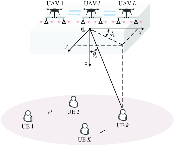
Figure 1: Wireless communication with a low-altitude UAV swarm enabled two-level MA system.

As illustrated in Fig. 1, we consider a low-altitude UAV swarm enabled wireless communication system, where $L$ UAVs cooperatively serve $K$ single-antenna ground UEs. Each UAV is equipped with a linear MA array with $M$ antenna elements, while a flexible two-level MA system is formed by dynamically moving each UAV and the positions of its individual MAs. Without loss of generality, we consider a 3D Cartesian coordinate system, where the location of UE $k$ is denoted as ${\bf w}_{\lx@text@underscore}k=\left[{{x_{\lx@text@underscore}k},{y_{\lx@text@underscore}k},0}\right]^{T}$, $k\in{\cal K}$, with ${\cal K}\triangleq\left[1,\cdots,K\right]$. Let the first antenna be the reference point for each UAV, with its coordinate for UAV $l$ denoted as ${{\bf{q}}_{\lx@text@underscore}l}={\left[{{x_{\lx@text@underscore}l},{y_{\lx@text@underscore}l},{z_{\lx@text@underscore}l}}\right]^{T}}$, $1\leq l\leq L$. The coordinate of antenna $m$ for UAV $l$ is ${{\bf{q}}_{\lx@text@underscore}{l,m}}={{\bf{q}}_{\lx@text@underscore}l}+{{\bf{b}}_{\lx@text@underscore}{l,m}}$, where ${{\bf{b}}_{\lx@text@underscore}{l,m}}\triangleq{\left[{{{b_{\lx@text@underscore}{l,m}}},0,0}\right]^{T}}$ and we assume ${b_{\lx@text@underscore}{l,1}}=0$, $\forall l$, without loss of generality. As such, position of antenna $m$ can be dynamically changed by adjusting ${b_{\lx@text@underscore}{l,m}}$ for UAV $l$. This thus enables a two-level MA system, realized by the joint control of UAVs’ movement and their individual antennas’ movement.

In practice, the collision avoidance constraints need to be satisfied by UAVs, which is given by [3]

$$\left\|{{{\bf{q}}_{\lx@text@underscore}l}-{{\bf{q}}_{\lx@text@underscore}{l^{\prime}}}}\right\|\geq{d_{\lx@text@underscore}{\min}},\ \forall l,l^{\prime}\neq l,$$ (1)

where $d_{\lx@text@underscore}{\min}$ denotes the minimum distance to avoid the collision between UAVs. Besides, to avoid the mutual coupling between adjacent MA elements at each UAV, the minimum distance ${\tilde{d}}_{\lx@text@underscore}{\min}$ is required, which yields the following constraints,

$$\left\|{{{\bf{q}}_{\lx@text@underscore}{l,m}}-{{\bf{q}}_{\lx@text@underscore}{l,m^{\prime}}}}\right\|=\left|{{b_{\lx@text@underscore}{l,m}}-{b_{\lx@text@underscore}{l,m^{\prime}}}}\right|\geq{{\tilde{d}}_{\lx@text@underscore}{\min}},\forall l,m,m^{\prime}\neq m,$$ (2)

where ${\tilde{d}}_{\lx@text@underscore}{\min}$ is in practice much smaller than $d_{\lx@text@underscore}{\min}$.

Let ${{\bf{q}}_{\lx@text@underscore}r}={\left[{{x_{\lx@text@underscore}r},{y_{\lx@text@underscore}r},{z_{\lx@text@underscore}r}}\right]^{T}}$ denote the reference location for the $L$ UAVs. We consider the far-field uniform plane wave (UPW) model for the channels between UAVs and ground UEs. Moreover, let ${{\bm{\kappa}}_{\lx@text@underscore}k}={\left[{{\Phi_{\lx@text@underscore}k},{\Psi_{\lx@text@underscore}k},{\Theta_{\lx@text@underscore}k}}\right]^{T}}$ denote the wave propagation direction from ${\bf q}_{\lx@text@underscore}r$ to UE $k$, with ${\Phi_{\lx@text@underscore}k}\triangleq\sin{\theta_{\lx@text@underscore}k}\cos{\phi_{\lx@text@underscore}k}$, ${\Psi_{\lx@text@underscore}k}\triangleq\sin{\theta_{\lx@text@underscore}k}\sin{\phi_{\lx@text@underscore}k}$, and ${\Theta_{\lx@text@underscore}k}\triangleq\cos{\theta_{\lx@text@underscore}k}$, respectively, where ${{\theta_{\lx@text@underscore}k}}$ and ${{\phi_{\lx@text@underscore}k}}$ denote the elevation and azimuth angles of arrival (AoAs), respectively, as illustrated in Fig. 1. The difference of the wavefront propagation distance between ${\bf q}_{\lx@text@underscore}r$ and ${{\bf{q}}_{\lx@text@underscore}{l,m}}$ for UE $k$ is

$${\varphi_{\lx@text@underscore}k}\left({{{\bf{q}}_{\lx@text@underscore}{l,m}}}\right) ={\bm{\kappa}}_{\lx@text@underscore}k^{T}\left({{{\bf{q}}_{\lx@text@underscore}{l,m}}-{{\bf{q}}_{\lx@text@underscore}r}}\right)=\left({{x_{\lx@text@underscore}l}+{b_{\lx@text@underscore}{l,m}}}\right){\Phi_{\lx@text@underscore}k}$$ (3)

$$\ \ \ +{y_{\lx@text@underscore}l}{\Psi_{\lx@text@underscore}k}+{z_{\lx@text@underscore}l}{\Theta_{\lx@text@underscore}k}-{\bm{\kappa}}_{\lx@text@underscore}k^{T}{{\bf{q}}_{\lx@text@underscore}r}.$$

Note that the communication links between UAVs and ground UEs are of high probability to be over LoS channels in practice. The receive array response vector of UAV $l$ for UE $k$ is given by

$${{\bf{a}}_{\lx@text@underscore}{k,l}}\left({\left\{{{{\bf{q}}_{\lx@text@underscore}{l,m}},\forall m}\right\}}\right)={\left[{{e^{{\rm{j}}\frac{{2\pi}}{\lambda}{\varphi_{\lx@text@underscore}k}\left({{{\bf{q}}_{\lx@text@underscore}{l,1}}}\right)}},\cdots,{e^{{\rm{j}}\frac{{2\pi}}{\lambda}{\varphi_{\lx@text@underscore}k}\left({{{\bf{q}}_{\lx@text@underscore}{l,M}}}\right)}}}\right]^{T}}.$$ (4)

Moreover, the $L$ UAVs cooperate to form an $LM$-element distributed antenna array, and thus the channel from the UAV swarm enabled MA system to UE $k$ is

$${{\bf{h}}_{\lx@text@underscore}k}\left({\left\{{{{\bf{q}}_{\lx@text@underscore}{l,m}},\forall l,m}\right\}}\right)={\alpha_{\lx@text@underscore}k}{{\bf{a}}_{\lx@text@underscore}k}\left({\left\{{{{\bf{q}}_{\lx@text@underscore}{l,m}},\forall l,m}\right\}}\right),$$ (5)

where ${\alpha_{\lx@text@underscore}k}=\sqrt{{\beta_{\lx@text@underscore}0}}/{d_{\lx@text@underscore}{r,k}}$ denotes the channel gain of UE $k$, with ${\beta_{\lx@text@underscore}0}$ being the channel power at the reference distance of ${d_{\lx@text@underscore}0}=1$ m and ${d_{\lx@text@underscore}{r,k}}=\left\|{{{\bf{w}}_{\lx@text@underscore}k}-{{\bf{q}}_{\lx@text@underscore}r}}\right\|$ being the distance between ${\bf q}_{\lx@text@underscore}r$ and ${\bf w}_{\lx@text@underscore}k$, respectively. Besides, ${{\bf{a}}_{\lx@text@underscore}k}\left({\left\{{{{\bf{q}}_{\lx@text@underscore}{l,m}},\forall l,m}\right\}}\right)\in{\mathbb{C}}^{LM\times 1}$ denotes the receive array response vector of UE $k$, given by

$${{\bf{a}}_{\lx@text@underscore}k}\left({\left\{{{{\bf{q}}_{\lx@text@underscore}{l,m}},\forall l,m}\right\}}\right)=\left[{{\bf{a}}_{\lx@text@underscore}{k,1}^{T}\left({\left\{{{{\bf{q}}_{\lx@text@underscore}{1,m}},\forall m}\right\}}\right),\cdots,}\right.$$ (6)

$${\left.{{\bf{a}}_{\lx@text@underscore}{k,L}^{T}\left({\left\{{{{\bf{q}}_{\lx@text@underscore}{L,m}},\forall m}\right\}}\right)}\right]^{T}}.$$

In the following, for brevity, we use the notations ${{\bf{h}}_{\lx@text@underscore}k}$, ${{\bf{a}}_{\lx@text@underscore}k}$ and ${{\bf{a}}_{\lx@text@underscore}{k,l}}$ to replace ${{\bf{h}}_{\lx@text@underscore}k}\left({\left\{{{{\bf{q}}_{\lx@text@underscore}{l,m}},\forall l,m}\right\}}\right)$, ${{\bf{a}}_{\lx@text@underscore}k}\left({\left\{{{{\bf{q}}_{\lx@text@underscore}{l,m}},\forall l,m}\right\}}\right)$ and ${{\bf{a}}_{\lx@text@underscore}{k,l}}\left({\left\{{{{\bf{q}}_{\lx@text@underscore}{l,m}},\forall m}\right\}}\right)$, respectively.

Denote by ${s_{\lx@text@underscore}k}$ the independent and identically distributed (i.i.d.) information-bearing symbol of UE $k$, with ${\mathbb{E}}[{{{\left|{{s_{\lx@text@underscore}k}}\right|}^{2}}}]=1$. To detect its symbol, the receive beamforming ${{\bf{v}}_{\lx@text@underscore}k}\in{\mathbb{C}}^{LM\times 1}$ is applied at the UAV swarm enabled MA system, with $\left\|{{\bf{v}}_{\lx@text@underscore}k}\right\|=1$. Thus, the resulting signal of UE $k$ after applying the receive beamforming is

$${y_{\lx@text@underscore}k}={\bf{v}}_{\lx@text@underscore}k^{H}{{\bf{h}}_{\lx@text@underscore}k}\sqrt{{P_{\lx@text@underscore}k}}{s_{\lx@text@underscore}k}+{\bf{v}}_{\lx@text@underscore}k^{H}\sum\limits_{\lx@text@underscore}{i=1,i\neq k}^{K}{{{\bf{h}}_{\lx@text@underscore}i}\sqrt{{P_{\lx@text@underscore}i}}{s_{\lx@text@underscore}i}}+{\bf{v}}_{\lx@text@underscore}k^{H}{\bf{z}},$$ (7)

where ${{P_{\lx@text@underscore}i}}$, $i=1,\cdots,K$, denotes the transmit power of UE $i$, ${\bf{z}}\sim{\cal CN}\left({{\bf{0}},{\sigma^{2}}{{\bf{I}}_{\lx@text@underscore}{LM}}}\right)$, with each element denoting the i.i.d. additive white Gaussian noise (AWGN) with zero mean and power ${\sigma^{2}}$.

The resulting SINR for UE $k$ is

$${\gamma_{\lx@text@underscore}k}=\frac{{{{\bar{P}}_{\lx@text@underscore}k}{{\left|{{\bf{v}}_{\lx@text@underscore}k^{H}{{\bf{h}}_{\lx@text@underscore}k}}\right|}^{2}}}}{{\sum\limits_{\lx@text@underscore}{i=1,i\neq k}^{K}{{{\bar{P}}_{\lx@text@underscore}i}{{\left|{{\bf{v}}_{\lx@text@underscore}k^{H}{{\bf{h}}_{\lx@text@underscore}i}}\right|}^{2}}}+1}}=\frac{{{{\bar{P}}_{\lx@text@underscore}k}{\bf{v}}_{\lx@text@underscore}k^{H}{{\bf{h}}_{\lx@text@underscore}k}{\bf{h}}_{\lx@text@underscore}k^{H}{{\bf{v}}_{\lx@text@underscore}k}}}{{{\bf{v}}_{\lx@text@underscore}k^{H}{{\bf{C}}_{\lx@text@underscore}k}{{\bf{v}}_{\lx@text@underscore}k}}},$$ (8)

where ${{\bf{C}}_{\lx@text@underscore}k}\triangleq{{\bf{I}}_{\lx@text@underscore}{LM}}+\sum\nolimits_{\lx@text@underscore}{i=1,i\neq k}^{K}{{{\bar{P}}_{\lx@text@underscore}i}{{\bf{h}}_{\lx@text@underscore}i}{\bf{h}}_{\lx@text@underscore}i^{H}}$ denotes the interference-plus-noise covariance matrix with respect to (w.r.t.) UE $k$, and ${{\bar{P}}_{\lx@text@underscore}i}\triangleq{P_{\lx@text@underscore}i}/{\sigma^{2}}$. The achievable rate of UE $k$ is

$${R_{\lx@text@underscore}k}={\log_{\lx@text@underscore}2}\left({1+{\gamma_{\lx@text@underscore}k}}\right).$$ (9)

Our objective is to maximize the minimum achievable rate over $K$ UEs, by jointly optimizing the 3D UAV swarm placement positions ${\bf{Q}}=\left\{{{{\bf{q}}_{\lx@text@underscore}l},\forall l}\right\}$, the local positions of MAs at all UAVs ${\bf{B}}=\left\{{{b_{\lx@text@underscore}{l,m}},\forall l,m=2,\cdots,M}\right\}$, and receive beamforming for all UEs ${\bf{V}}=\left\{{{{\bf{v}}_{\lx@text@underscore}k},\forall k}\right\}$. This optimization problem can be formulated as

$$\left({\rm{P1}}\right)\ \ \mathop{\max}\limits_{\lx@text@underscore}{{\bf{Q}},{\bf{B}},{\bf{V}}}\ \mathop{\min}\limits_{\lx@text@underscore}{k\in{\cal K}}\ {R_{\lx@text@underscore}k}$$ (10)

$${\rm{s.t.}} \ {{\bf{q}}_{\lx@text@underscore}l}\in{\cal C},\ \forall l,$$ (10a)

$$\ {\left\|{{{\bf{q}}_{\lx@text@underscore}l}-{{\bf{q}}_{\lx@text@underscore}{l^{\prime}}}}\right\|^{2}}\geq d_{\lx@text@underscore}{\min}^{2},\ \forall l,l^{\prime}\neq l,$$ (10b)

$$\ {b_{\lx@text@underscore}{l,m}}\in{\tilde{\cal C}},\ \forall l,m,$$ (10c)

$$\ {\left|{{b_{\lx@text@underscore}{l,m}}-{b_{\lx@text@underscore}{l,m^{\prime}}}}\right|^{2}}\geq\tilde{d}_{\lx@text@underscore}{\min}^{2},\ \forall l,m,m^{\prime}\neq m,$$ (10d)

$$\ \left\|{{{\bf{v}}_{\lx@text@underscore}k}}\right\|=1,\ \forall k,$$ (10e)

where $\cal C$ denotes the movable region of UAVs, ${\tilde{\cal C}}$ denotes the (local) movable region of MAs at each UAV, and the collision and mutual coupling avoidance constraints in (1) and (2) have been replaced by their equivalent quadratic forms, i.e., (10b) and (10d), respectively. Problem (P1) is challenging to be directly solved due to the non-concave objective function and (some) non-convex constraints. Besides, the optimization variables ${\bf Q}$, ${\bf B}$ and ${\bf V}$ are intricately coupled in the objective function, which makes their joint optimization a challenging task.

III Special Case of Single-Antenna UAV

In this section, to gain useful insights, we first consider the special case of single-antenna UAV, i.e., $M=1$, where (P1) is reduced to

$$\mathop{\max}\limits_{\lx@text@underscore}{{\bf{Q}},{\bf{V}}} \ \mathop{\min}\limits_{\lx@text@underscore}{k\in{\cal K}}\ {R_{\lx@text@underscore}k}$$ (11)

$${\rm{s.t.}} \ {{\bf{q}}_{\lx@text@underscore}l}\in{\cal C},\ \forall l,$$

$$\ {\left\|{{{\bf{q}}_{\lx@text@underscore}l}-{{\bf{q}}_{\lx@text@underscore}{l^{\prime}}}}\right\|^{2}}\geq d_{\lx@text@underscore}{\min}^{2},\ \forall l,l^{\prime}\neq l,$$

$$\ \left\|{{{\bf{v}}_{\lx@text@underscore}k}}\right\|=1,\ \forall k.$$

In the following, the cases of one single UE, two UEs and arbitrary number of UEs are studied, respectively.

III-A Single UE and Two UEs

For the single UE communication, the receive signal in (7) reduces to

$$y={{\bf{v}}^{H}}{\bf{h}}\sqrt{P}s+{{\bf{v}}^{H}}{\bf{z}},$$ (12)

where the UE index is omitted for brevity. By applying the optimal MRC beamforming, i.e., ${\bf{v}}={\bf{h}}/\left\|{{\bf{h}}}\right\|$, the resulting SNR is given by

$$\gamma=\bar{P}{\left\|{{\bf{h}}}\right\|^{2}}=\bar{P}{\left|\alpha\right|^{2}}L,$$ (13)

which only depends on the number of UAVs $L$, irrespective of the geometry formed by the UAV swarm enabled MA system. As a result, any UAV swarm placement satisfying the collision avoidance constraint can achieve the maximum achievable rate.

Next, we consider the classic MRC, zero-forcing (ZF) and minimum mean-square error (MMSE) beamforming schemes for the case of two UEs. Denote by ${\xi_{\lx@text@underscore}{k,k^{\prime}}}\triangleq\frac{{{{\left|{{\bf{h}}_{\lx@text@underscore}k^{H}{{\bf{h}}_{\lx@text@underscore}{k^{\prime}}}}\right|}^{2}}}}{{{{\left\|{{{\bf{h}}_{\lx@text@underscore}k}}\right\|}^{2}}{{\left\|{{{\bf{h}}_{\lx@text@underscore}{k^{\prime}}}}\right\|}^{2}}}}$ the channel’s squared-correlation coefficient between UEs $k$ and $k^{\prime}$, where $k,k^{\prime}=1,2$ and $k\neq k^{\prime}$. Under the far-field UPW model, we have ${\left\|{{{\bf{h}}_{\lx@text@underscore}k}}\right\|^{2}}={\left|{{\alpha_{\lx@text@underscore}k}}\right|^{2}}L$. The resulting SINR/SNR of UE $k$ after applying the three beamforming schemes are respectively given by [34, 35]

$${\gamma_{\lx@text@underscore}{{\rm{MRC}},k}}={{\bar{P}}_{\lx@text@underscore}k}{\left|{{\alpha_{\lx@text@underscore}k}}\right|^{2}}L\left({1-\frac{{{{\bar{P}}_{\lx@text@underscore}{k^{\prime}}}{{\left|{{\alpha_{\lx@text@underscore}{k^{\prime}}}}\right|}^{2}}L{\xi_{\lx@text@underscore}{k,k^{\prime}}}}}{{{{\bar{P}}_{\lx@text@underscore}{k^{\prime}}}{{\left|{{\alpha_{\lx@text@underscore}{k^{\prime}}}}\right|}^{2}}L{\xi_{\lx@text@underscore}{k,k^{\prime}}}+1}}}\right),$$ (14)

$${\gamma_{\lx@text@underscore}{{\rm{ZF}},k}}={{\bar{P}}_{\lx@text@underscore}k}{\left|{{\alpha_{\lx@text@underscore}k}}\right|^{2}}L\left({1-{\xi_{\lx@text@underscore}{k,k^{\prime}}}}\right),$$ (15)

$${\gamma_{\lx@text@underscore}{{\rm{MMSE}},k}}={{\bar{P}}_{\lx@text@underscore}k}{\left|{{\alpha_{\lx@text@underscore}k}}\right|^{2}}L\left({1-\frac{{{{\bar{P}}_{\lx@text@underscore}{k^{\prime}}}{{\left|{{\alpha_{\lx@text@underscore}{k^{\prime}}}}\right|}^{2}}L{\xi_{\lx@text@underscore}{k,k^{\prime}}}}}{{{{\bar{P}}_{\lx@text@underscore}{k^{\prime}}}{{\left|{{\alpha_{\lx@text@underscore}{k^{\prime}}}}\right|}^{2}}L+1}}}\right).$$ (16)

It is observed from (14)-(16) that the SINRs of MRC, ZF, and MMSE beamforming depend on the coefficient ${\xi_{\lx@text@underscore}{k,k^{\prime}}}$, and a larger SINR can be achieved as ${\xi_{\lx@text@underscore}{k,k^{\prime}}}$ decreases. Moreover, the terms ${\frac{{{{\bar{P}}_{\lx@text@underscore}{k^{\prime}}}{{\left|{{\alpha_{\lx@text@underscore}{k^{\prime}}}}\right|}^{2}}L{\xi_{\lx@text@underscore}{k,k^{\prime}}}}}{{{{\bar{P}}_{\lx@text@underscore}{k^{\prime}}}{{\left|{{\alpha_{\lx@text@underscore}{k^{\prime}}}}\right|}^{2}}L{\xi_{\lx@text@underscore}{k,k^{\prime}}}+1}}}$, ${\xi_{\lx@text@underscore}{k,k^{\prime}}}$, and ${\frac{{{{\bar{P}}_{\lx@text@underscore}{k^{\prime}}}{{\left|{{\alpha_{\lx@text@underscore}{k^{\prime}}}}\right|}^{2}}L{\xi_{\lx@text@underscore}{k,k^{\prime}}}}}{{{{\bar{P}}_{\lx@text@underscore}{k^{\prime}}}{{\left|{{\alpha_{\lx@text@underscore}{k^{\prime}}}}\right|}^{2}}L+1}}}$ in (14)-(16) account for the SNR loss factors for UE $k$ due to applying the MRC, ZF, and MMSE beamforming schemes, respectively. By substituting (5) into ${\xi_{\lx@text@underscore}{k,k^{\prime}}}$, we have

$${\xi_{\lx@text@underscore}{k,k^{\prime}}}=\frac{1}{{{L^{2}}}}{\left|{{\bf{a}}_{\lx@text@underscore}k^{H}{{\bf{a}}_{\lx@text@underscore}{k^{\prime}}}}\right|^{2}}.$$ (17)

Based on the above observation, for the case of two UEs, we aim to minimize the channels’ squared-correlation coefficient, which can be formulated as

$$\mathop{\min}\limits_{\lx@text@underscore}{\bf{Q}} \ \frac{1}{{{L^{2}}}}{\left|{{\bf{a}}_{\lx@text@underscore}k^{H}{{\bf{a}}_{\lx@text@underscore}{k^{\prime}}}}\right|^{2}}$$ (18)

$${\rm{s.t.}} \ {{\bf{q}}_{\lx@text@underscore}l}\in{\cal C},\ \forall l,$$

$$\ {\left\|{{{\bf{q}}_{\lx@text@underscore}l}-{{\bf{q}}_{\lx@text@underscore}{l^{\prime}}}}\right\|^{2}}\geq d_{\lx@text@underscore}{\min}^{2},\ \forall l,l^{\prime}\neq l.$$

To tackle problem (18), we first study the property of the objective function. By substituting (6) into the objective function, we have

$$\frac{1}{{{L^{2}}}}{\left|{{\bf{a}}_{\lx@text@underscore}k^{H}{{\bf{a}}_{\lx@text@underscore}{k^{\prime}}}}\right|^{2}} =\frac{1}{{{L^{2}}}}{\left|{\sum\limits_{\lx@text@underscore}{l=1}^{L}{{e^{-{\rm{j}}\frac{{2\pi}}{\lambda}\left({{\varphi_{\lx@text@underscore}k}\left({{{\bf{q}}_{\lx@text@underscore}l}}\right)-{\varphi_{\lx@text@underscore}{k^{\prime}}}\left({{{\bf{q}}_{\lx@text@underscore}l}}\right)}\right)}}}}\right|^{2}}$$ (19)

$$=\frac{1}{{{L^{2}}}}{\left|{\sum\limits_{\lx@text@underscore}{l=1}^{L}{{e^{-{\rm{j}}\frac{{2\pi}}{\lambda}{{\left({{{\bm{\kappa}}_{\lx@text@underscore}k}-{{\bm{\kappa}}_{\lx@text@underscore}{k^{\prime}}}}\right)}^{T}}{{\bf{q}}_{\lx@text@underscore}l}}}}}\right|^{2}}.$$

By letting ${\nu_{\lx@text@underscore}{\min}}={\left\lceil{L{d_{\lx@text@underscore}{\min}}\left\|{{{\bm{\kappa}}_{\lx@text@underscore}k}-{{\bm{\kappa}}_{\lx@text@underscore}{k^{\prime}}}}\right\|/\lambda-1}\right\rceil}$, we obtain the following theorem.

Theorem 1

An optimal solution to (18) that achieves zero objective value is

$${{\bf{q}}_{\lx@text@underscore}l}={{\bf{q}}_{\lx@text@underscore}1}+\left({l-1}\right)\frac{{\left({{\varsigma^{\star}}+1/L}\right)\lambda}}{{{{\left\|{{{\bm{\kappa}}_{\lx@text@underscore}k}-{{\bm{\kappa}}_{\lx@text@underscore}{k^{\prime}}}}\right\|}^{2}}}}\left({{{\bm{\kappa}}_{\lx@text@underscore}k}-{{\bm{\kappa}}_{\lx@text@underscore}{k^{\prime}}}}\right),$$ (20)

where ${{\bf{q}}_{\lx@text@underscore}1}$ can be any vector to guarantee ${{\bf{q}}_{\lx@text@underscore}l}\in{\cal C}$, $\forall l$, and ${\varsigma^{\star}}$ is given by

$${\varsigma^{\star}}=\left\{\begin{split}&\frac{{{\nu_{\lx@text@underscore}{\min}}}}{L},\ \ \ \ \ \ {\rm if}\ \bmod\left({{\nu_{\lx@text@underscore}{\min}}+1,L}\right)\neq 0,\\ &\frac{{{\nu_{\lx@text@underscore}{\min}}+1}}{L},\ {\rm otherwise}.\end{split}\right.$$ (21)

Proof:

Please refer to Appendix A. ∎

Note that Theorem 1 extends the 1D result in [23] to the general 3D placement, and the derived closed-form solution ${\varsigma^{\star}}$ can be a fraction, which removes the requirement of being an integer imposed in [23]. Moreover, UAV placement position ${{\bf{q}}_{\lx@text@underscore}l}\in{\cal C}$, $\forall l$, can be satisfied when $\left\|{{{\bf{q}}_{\lx@text@underscore}L}-{{\bf{q}}_{\lx@text@underscore}1}}\right\|=\frac{{\left({L-1}\right)\left({{\varsigma^{\star}}+1/L}\right)\lambda}}{{\left\|{{{\bm{\kappa}}_{\lx@text@underscore}k}-{{\bm{\kappa}}_{\lx@text@underscore}{k^{\prime}}}}\right\|}}$ is no greater than the maximum distance between any two points in ${\cal C}$.

With (20) and (21), we have ${\xi_{\lx@text@underscore}{k,k^{\prime}}}=0$, and ${\gamma_{\lx@text@underscore}{{\rm{MRC}},k}}={\gamma_{\lx@text@underscore}{{\rm{ZF}},k}}\ ={\gamma_{\lx@text@underscore}{{\rm{MMSE}},k}}={{\bar{P}}_{\lx@text@underscore}k}{\left\|{{{\bf{h}}_{\lx@text@underscore}k}}\right\|^{2}}={{\bar{P}}_{\lx@text@underscore}k}{\left|{{\alpha_{\lx@text@underscore}k}}\right|^{2}}L$, i.e., they are identical to the single UE SNR without IUI. Thus, an IUI-free communication can be achieved with the UAV swarm enabled MA system, by setting the UAVs’ static positions according to Theorem 1. It is worth noting that the inter-UAV distance is $\frac{{\left|{{\varsigma^{\star}}+1/L}\right|\lambda}}{{\left\|{{{\bm{\kappa}}_{\lx@text@underscore}k}-{{\bm{\kappa}}_{\lx@text@underscore}{k^{\prime}}}}\right\|}}\geq d_{\lx@text@underscore}{\min}$, where the minimum distance $d_{\lx@text@underscore}{\min}$ is in general much larger than half wavelength. Thus, the UAV swarm forms a USA for the IUI-free communication. Moreover, the objective function in (P1) is given by

$$\mathop{\min}\limits_{\lx@text@underscore}{k\in K}{\log_{\lx@text@underscore}2}\left({1+{{\bar{P}}_{\lx@text@underscore}k}{{\left|{{\alpha_{\lx@text@underscore}k}}\right|}^{2}}L}\right).$$ (22)

It can be observed that the UAV swarm enabled MA system not only completely eliminates the IUI, but also achieves the full beamforming gain at each UE, in terms of the number of UAVs $L$ in (22), without suffering from any performance loss as in the traditional FPA system [34].

III-B Arbitrary Number of UEs

In this subsection, for arbitrary number of UEs, we propose an alternating optimization algorithm to solve problem (11) sub-optimally, where the receive beamforming and each UAV placement position are optimized alternately in an iterative manner.

III-B1 Optimization of ${\bf V}$ With Given ${\bf Q}$

For given UAV swarm placement positions ${\bf Q}$, the receive beamforming optimization problem in (11) is expressed as

$$\mathop{\max}\limits_{\lx@text@underscore}{\bf{V}} \ \mathop{\min}\limits_{\lx@text@underscore}{k\in{\cal K}}\ {R_{\lx@text@underscore}k}$$ (23)

$${\rm{s.t.}} \ \left\|{{{\bf{v}}_{\lx@text@underscore}k}}\right\|=1,\ \forall k.$$

A closer look at (8) shows that the receive beamforming ${{\bf{v}}_{\lx@text@underscore}k}$ only impacts the SINR for UE $k$. Thus, problem (23) can be decomposed as $K$ parallel sub-problems. Specifically, the sub-problem for UE $k$ is written as

$$\mathop{\max}\limits_{\lx@text@underscore}{{\bf{v}}_{\lx@text@underscore}k} \ \ {\gamma_{\lx@text@underscore}k}$$ (24)

$${\rm{s.t.}} \ \left\|{{{\bf{v}}_{\lx@text@underscore}k}}\right\|=1.$$

Since the resulting SINR in (8) is a generalized Rayleigh quotient w.r.t. ${\bf{v}}_{\lx@text@underscore}k$, the optimal ${\bf{v}}_{\lx@text@underscore}k$ to (24) is given by the classical MMSE beamforming [46]:

$${\bf{v}}_{\lx@text@underscore}k^{\star}=\frac{{{\bf{C}}_{\lx@text@underscore}k^{-1}{{\bf{h}}_{\lx@text@underscore}k}}}{{\left\|{{\bf{C}}_{\lx@text@underscore}k^{-1}{{\bf{h}}_{\lx@text@underscore}k}}\right\|}},\ \forall n,k.$$ (25)

III-B2 Optimization of ${{\bf{q}}_{\lx@text@underscore}l}$ With Given ${\bf V}$ and $\left\{{{\bf{q}}_{\lx@text@underscore}{l^{\prime}},\forall l^{\prime}\neq l}\right\}$

For given ${\bf V}$ and $\left\{{{\bf{q}}_{\lx@text@underscore}{l^{\prime}},\forall l^{\prime}\neq l}\right\}$, the sub-problem of (11) for optimizing the placement position of UAV $l$ can be expressed as

$$\mathop{\max}\limits_{\lx@text@underscore}{{\bf{q}}_{\lx@text@underscore}l} \ \mathop{\min}\limits_{\lx@text@underscore}{k\in{\cal K}}{R_{\lx@text@underscore}k}$$ (26)

$${\rm{s.t.}} \ {{\bf{q}}_{\lx@text@underscore}l}\in{\cal C},$$

$${\left\|{{{\bf{q}}_{\lx@text@underscore}l}-{{\bf{q}}_{\lx@text@underscore}{l^{\prime}}}}\right\|^{2}}\geq d_{\lx@text@underscore}{\min}^{2},\ \forall l^{\prime}\neq l.$$

By introducing the slack variable $\rho$, problem (26) is equivalently written as

$$\mathop{\max}\limits_{\lx@text@underscore}{{\bf{q}}_{\lx@text@underscore}l,\rho} \ \rho$$ (27)

$${\rm{s.t.}} \ {R_{\lx@text@underscore}k}\geq\rho,\ \forall k\in{\cal K},$$ (27a)

$$\ {{\bf{q}}_{\lx@text@underscore}l}\in{\cal C},$$ (27b)

$$\ {\left\|{{{\bf{q}}_{\lx@text@underscore}l}-{{\bf{q}}_{\lx@text@underscore}{l^{\prime}}}}\right\|^{2}}\geq d_{\lx@text@underscore}{\min}^{2},\ \forall l^{\prime}\neq l.$$ (27c)

Moreover, to tackle the non-convexity of the constraint (27a), the slack variables $\left\{{{\eta_{\lx@text@underscore}k},{\mu_{\lx@text@underscore}k},\forall k}\right\}$ are introduced such that

$${e^{{\eta_{\lx@text@underscore}k}}}=1+\sum\limits_{\lx@text@underscore}{i=1}^{K}{{{\bar{P}}_{\lx@text@underscore}i}{{\left|{{\bf{v}}_{\lx@text@underscore}k^{H}{{\bf{h}}_{\lx@text@underscore}i}}\right|}^{2}}},$$ (28)

$${e^{{\mu_{\lx@text@underscore}k}}}=1+\sum\limits_{\lx@text@underscore}{i=1,i\neq k}^{K}{{{\bar{P}}_{\lx@text@underscore}i}{{\left|{{\bf{v}}_{\lx@text@underscore}k^{H}{{\bf{h}}_{\lx@text@underscore}i}}\right|}^{2}}}.$$ (29)

Thus, problem (27) is transformed into

$$\mathop{\max}\limits_{\lx@text@underscore}{{{\bf q}_{\lx@text@underscore}l},\rho,\left\{{{\eta_{\lx@text@underscore}k},{\mu_{\lx@text@underscore}k}}\right\}_{\lx@text@underscore}{k=1}^{K}}\ \ \rho$$ (30)

$${\rm{s.t.}} \ {\frac{{\ln\left({{e^{{\eta_{\lx@text@underscore}k}-{\mu_{\lx@text@underscore}k}}}}\right)}}{{\ln 2}}}\geq\rho,\ \forall k\in{\cal K},$$ (30a)

$${\sigma^{2}}+\sum\limits_{\lx@text@underscore}{i=1}^{K}{{P_{\lx@text@underscore}i}{{\left|{{\bf{v}}_{\lx@text@underscore}k^{H}{{\bf{h}}_{\lx@text@underscore}i}}\right|}^{2}}}\geq{\sigma^{2}}{e^{{\eta_{\lx@text@underscore}k}}},\ \forall k\in{\cal K},$$ (30b)

$${\sigma^{2}}+\sum\limits_{\lx@text@underscore}{i=1,i\neq k}^{K}{{P_{\lx@text@underscore}i}{{\left|{{\bf{v}}_{\lx@text@underscore}k^{H}{{\bf{h}}_{\lx@text@underscore}i}}\right|}^{2}}}\leq{\sigma^{2}}{e^{{\mu_{\lx@text@underscore}k}}},\ \forall k\in{\cal K},$$ (30c)

$${{\bf{q}}_{\lx@text@underscore}l}\in{\cal C},$$ (30d)

$${\left\|{{{\bf{q}}_{\lx@text@underscore}l}-{{\bf{q}}_{\lx@text@underscore}{l^{\prime}}}}\right\|^{2}}\geq d_{\lx@text@underscore}{\min}^{2},\ l^{\prime}\neq l.$$ (30e)

Note that problem (30) is still challenging to be solved since the constraints (30b), (30c) and (30e) are non-convex. To tackle this issue, the SCA technique [3] is applied in the following.

Let ${{\bf{\bar{h}}}_{\lx@text@underscore}{i,l}}\in{{\mathbb{C}}^{\left({L-1}\right)\times 1}}$ denote the resulting channel after removing ${h_{\lx@text@underscore}{i,l}}$ from ${{\bf{h}}_{\lx@text@underscore}i}$, and ${{\bf{\bar{v}}}_{\lx@text@underscore}{k,l}}\in{{\mathbb{C}}^{\left({L-1}\right)\times 1}}$ denote the resulting beamforming vector after removing ${v_{\lx@text@underscore}{k,l}}$ from ${{\bf{v}}_{\lx@text@underscore}k}$, where ${h_{\lx@text@underscore}{i,l}}$ and ${v_{\lx@text@underscore}{k,l}}$ denote the $l$-th element of ${{\bf{h}}_{\lx@text@underscore}i}$ and ${{\bf{v}}_{\lx@text@underscore}k}$, respectively. Then, ${f_{\lx@text@underscore}{k,i}}\triangleq{\left|{{\bf{v}}_{\lx@text@underscore}k^{H}{{\bf{h}}_{\lx@text@underscore}i}}\right|^{2}}$ can be expressed as

$${f_{\lx@text@underscore}{k,i}} ={\bf{h}}_{\lx@text@underscore}i^{H}{{\bf{v}}_{\lx@text@underscore}k}{\bf{v}}_{\lx@text@underscore}k^{H}{{\bf{h}}_{\lx@text@underscore}i}=\underbrace{\sum\limits_{\lx@text@underscore}{l^{\prime}=1,l^{\prime}\neq l}^{L}{2{\mathop{\rm Re}\nolimits}\left\{{h_{\lx@text@underscore}{i,l}^{*}{V_{\lx@text@underscore}{k,l,l^{\prime}}}{h_{\lx@text@underscore}{i,l^{\prime}}}}\right\}}}_{\lx@text@underscore}{{g_{\lx@text@underscore}{k,i,l}}}$$ (31)

$$+\underbrace{{{\left|{{\alpha_{\lx@text@underscore}i}}\right|}^{2}}{V_{\lx@text@underscore}{k,l,l}}+{\bf{\bar{h}}}_{\lx@text@underscore}{i,l}^{H}{{\bf{\bar{V}}}_{\lx@text@underscore}{k,l,l}}{{\bf{\bar{h}}}_{\lx@text@underscore}{i,l}}}_{\lx@text@underscore}{{{\bar{g}}_{\lx@text@underscore}{k,i,l}}},$$

where ${V_{\lx@text@underscore}{k,l,l^{\prime}}}\triangleq{v_{\lx@text@underscore}{k,l}}v_{\lx@text@underscore}{k,l^{\prime}}^{*}$ and ${{\bf{\bar{V}}}_{\lx@text@underscore}{k,l,l}}\in{{\mathbb{C}}^{\left({L-1}\right)\times\left({L-1}\right)}}\triangleq{{\bf{\bar{v}}}_{\lx@text@underscore}{k,l}}{\bf{\bar{v}}}_{\lx@text@underscore}{k,l}^{H}$, and ${\bar{g}}_{\lx@text@underscore}{k,i,l}$ is independent of ${{\bf{q}}_{\lx@text@underscore}l}$. By substituting ${h_{\lx@text@underscore}{i,l}}={\alpha_{\lx@text@underscore}i}{e^{{\rm{j}}\frac{{2\pi}}{\lambda}{\varphi_{\lx@text@underscore}i}\left({{{\bf{q}}_{\lx@text@underscore}l}}\right)}}$ into ${g_{\lx@text@underscore}{k,i,l}}$, we have

$${g_{\lx@text@underscore}{k,i,l}}=\sum\limits_{\lx@text@underscore}{l^{\prime}=1,l^{\prime}\neq l}^{L}{2{{\left|{{\alpha_{\lx@text@underscore}i}}\right|}^{2}}{\rm{Re}}\left\{{{V_{\lx@text@underscore}{k,l,l^{\prime}}}{e^{-{\rm{j}}\frac{{2\pi}}{\lambda}\left({{\varphi_{\lx@text@underscore}i}\left({{{\bf{q}}_{\lx@text@underscore}l}}\right)-{\varphi_{\lx@text@underscore}i}\left({{{\bf{q}}_{\lx@text@underscore}{l^{\prime}}}}\right)}\right)}}}\right\}}$$ (32)

$$=\sum\limits_{\lx@text@underscore}{l^{\prime}=1,l^{\prime}\neq l}^{L}{2{{\left|{{\alpha_{\lx@text@underscore}i}}\right|}^{2}}\left|{{V_{\lx@text@underscore}{k,l,l^{\prime}}}}\right|}\cos\left({\frac{{2\pi}}{\lambda}{\bm{\kappa}}_{\lx@text@underscore}i^{T}\left({{{\bf{q}}_{\lx@text@underscore}l}-{{\bf{q}}_{\lx@text@underscore}{l^{\prime}}}}\right)-\angle{V_{\lx@text@underscore}{k,l,l^{\prime}}}}\right).$$

It is observed that (32) is neither convex nor concave with respect to ${{\bf q}_{\lx@text@underscore}l}$. To this end, two quadratic surrogate functions are respectively constructed to serve as the lower and upper bounds for ${g_{\lx@text@underscore}{k,i,l}}$, shown in the following lemma.

Lemma 1

The lower and upper bounds of ${g_{\lx@text@underscore}{k,i,l}}$ are respectively given by

$${g_{\lx@text@underscore}{k,i,l}} \geq{\left[{{g_{\lx@text@underscore}{k,i,l}}}\right]_{\lx@text@underscore}{\rm lb}}={g_{\lx@text@underscore}{k,i,l}}\left({{\bf{q}}_{\lx@text@underscore}l^{\left(j\right)}}\right)+\nabla{g_{\lx@text@underscore}{k,i,l}}{\left({{\bf{q}}_{\lx@text@underscore}l^{\left(j\right)}}\right)^{T}}\left({{{\bf{q}}_{\lx@text@underscore}l}-{\bf{q}}_{\lx@text@underscore}l^{\left(j\right)}}\right)$$ (33)

$$\ \ \ \ \ \ \ \ -\frac{{{\delta_{\lx@text@underscore}{k,i,l}}}}{2}{\left({{{\bf{q}}_{\lx@text@underscore}l}-{\bf{q}}_{\lx@text@underscore}l^{\left(j\right)}}\right)^{T}}\left({{{\bf{q}}_{\lx@text@underscore}l}-{\bf{q}}_{\lx@text@underscore}l^{\left(j\right)}}\right),$$

$${g_{\lx@text@underscore}{k,i,l}} \leq{\left[{{g_{\lx@text@underscore}{k,i,l}}}\right]_{\lx@text@underscore}{\rm ub}}={g_{\lx@text@underscore}{k,i,l}}\left({{\bf{q}}_{\lx@text@underscore}l^{\left(j\right)}}\right)+\nabla{g_{\lx@text@underscore}{k,i,l}}{\left({{\bf{q}}_{\lx@text@underscore}l^{\left(j\right)}}\right)^{T}}\left({{{\bf{q}}_{\lx@text@underscore}l}-{\bf{q}}_{\lx@text@underscore}l^{\left(j\right)}}\right)$$ (34)

$$\ \ \ \ \ \ \ \ +\frac{{{\delta_{\lx@text@underscore}{k,i,l}}}}{2}{\left({{{\bf{q}}_{\lx@text@underscore}l}-{\bf{q}}_{\lx@text@underscore}l^{\left(j\right)}}\right)^{T}}\left({{{\bf{q}}_{\lx@text@underscore}l}-{\bf{q}}_{\lx@text@underscore}l^{\left(j\right)}}\right),$$

where ${\delta_{\lx@text@underscore}{k,i,l}}=\frac{{8{\pi^{2}}}}{{{\lambda^{2}}}}{\left|{{\alpha_{\lx@text@underscore}i}}\right|^{2}}\sum\nolimits_{\lx@text@underscore}{l^{\prime}=1,l^{\prime}\neq l}^{L}{\left|{V_{\lx@text@underscore}{k,l,l^{\prime}}}\right|}$, ${{\bf{q}}_{\lx@text@underscore}l^{\left(j\right)}}$ denotes the resulting placement position of UAV $l$ in the $j$-th iteration, and $\nabla{g_{\lx@text@underscore}{k,i,l}}({{\bf{q}}_{\lx@text@underscore}l^{\left(j\right)}})$ denotes the gradient of ${{g_{\lx@text@underscore}{k,i,l}}}$ over ${\bf{q}}_{\lx@text@underscore}l^{\left(j\right)}$.

Proof:

Please refer to Appendix B. ∎

With Lemma 1, the lower and upper bounds of the function ${f_{\lx@text@underscore}{k,i}}$ are

$${f_{\lx@text@underscore}{k,i}}\geq{\left[{{f_{\lx@text@underscore}{k,i}}}\right]_{\lx@text@underscore}{\rm lb}}\triangleq{\left[{{g_{\lx@text@underscore}{k,i,l}}}\right]_{\lx@text@underscore}{\rm lb}}+{{\bar{g}}_{\lx@text@underscore}{k,i,l}},$$ (35)

$${f_{\lx@text@underscore}{k,i}}\leq{\left[{{f_{\lx@text@underscore}{k,i}}}\right]_{\lx@text@underscore}{\rm ub}}\triangleq{\left[{{g_{\lx@text@underscore}{k,i,l}}}\right]_{\lx@text@underscore}{\rm ub}}+{{\bar{g}}_{\lx@text@underscore}{k,i,l}},$$ (36)

which are concave and convex with respect to ${{\bf{q}}_{\lx@text@underscore}l}$, respectively.

Moreover, to tackle the non-convexity of ${e^{{\mu_{\lx@text@underscore}k}}}$ on the right-hand-side (RHS) of (30c), let $\mu_{\lx@text@underscore}k^{\left(j\right)}$ denote the resulting variable in the $j$-th iteration; then the convex function ${e^{{\mu_{\lx@text@underscore}k}}}$ is lower-bounded by

$${e^{{\mu_{\lx@text@underscore}k}}}\geq{\left[{{e^{{\mu_{\lx@text@underscore}k}}}}\right]_{\lx@text@underscore}{{\rm{lb}}}}\triangleq{\mu_{\lx@text@underscore}k}{e^{\mu_{\lx@text@underscore}k^{\left(j\right)}}}+\left({1-\mu_{\lx@text@underscore}k^{\left(j\right)}}\right){e^{\mu_{\lx@text@underscore}k^{\left(j\right)}}}.$$ (37)

Similarly, for given ${\bf{q}}_{\lx@text@underscore}l^{\left(j\right)}$, the convex function ${\left\|{{{\bf{q}}_{\lx@text@underscore}l}-{{\bf{q}}_{\lx@text@underscore}{l^{\prime}}}}\right\|^{2}}$ on the left-hand-side (LHS) of (30e) is lower-bounded by [3]

$${\left\|{{{\bf{q}}_{\lx@text@underscore}l}-{{\bf{q}}_{\lx@text@underscore}{l^{\prime}}}}\right\|^{2}}\geq{\left[{{{\left\|{{{\bf{q}}_{\lx@text@underscore}l}-{{\bf{q}}_{\lx@text@underscore}{l^{\prime}}}}\right\|}^{2}}}\right]_{\lx@text@underscore}{{\rm{lb}}}}$$ (38)

$$\triangleq 2{\left({{\bf{q}}_{\lx@text@underscore}l^{\left(j\right)}-{{\bf{q}}_{\lx@text@underscore}{l^{\prime}}}}\right)^{T}}\left({{{\bf{q}}_{\lx@text@underscore}l}-{\bf{q}}_{\lx@text@underscore}l^{\left(j\right)}}\right)+{\left\|{{\bf{q}}_{\lx@text@underscore}l^{\left(j\right)}-{{\bf{q}}_{\lx@text@underscore}{l^{\prime}}}}\right\|^{2}}.$$

As a result, problem (30) is lower-bounded by the following problem for given $\{{{\bf{q}}_{\lx@text@underscore}l^{\left(j\right)},\mu_{\lx@text@underscore}k^{\left(j\right)}}\}$.

$$\mathop{\max}\limits_{\lx@text@underscore}{{{\bf{q}}_{\lx@text@underscore}l},\rho,\left\{{{\eta_{\lx@text@underscore}k},{\mu_{\lx@text@underscore}k}}\right\}_{\lx@text@underscore}{k=1}^{K}}\ \ \rho$$ (39)

$${\rm{s.t.}} \ {{\eta_{\lx@text@underscore}k}-{\mu_{\lx@text@underscore}k}}\geq\rho\ln 2,\ \forall k\in{\cal K},$$

$${\sigma^{2}}+\sum\limits_{\lx@text@underscore}{i=1}^{K}{{P_{\lx@text@underscore}i}{{\left[{{f_{\lx@text@underscore}{ki}}}\right]}_{\lx@text@underscore}{{\rm{lb}}}}}\geq{\sigma^{2}}{e^{{\eta_{\lx@text@underscore}k}}},\ \forall k\in{\cal K},$$

$${\sigma^{2}}+\sum\limits_{\lx@text@underscore}{i=1,i\neq k}^{K}{{P_{\lx@text@underscore}i}{{\left[{{f_{\lx@text@underscore}{ki}}}\right]}_{\lx@text@underscore}{{\rm{ub}}}}}\leq{\sigma^{2}}{\left[{{e^{{\mu_{\lx@text@underscore}k}}}}\right]_{\lx@text@underscore}{{\rm{lb}}}},\ \forall k\in{\cal K},$$

$${{\bf{q}}_{\lx@text@underscore}l}\in{\cal C},$$

$${\left[{{{\left\|{{{\bf{q}}_{\lx@text@underscore}l}-{{\bf{q}}_{\lx@text@underscore}{l^{\prime}}}}\right\|}^{2}}}\right]_{\lx@text@underscore}{{\rm{lb}}}}\geq d_{\lx@text@underscore}{\min}^{2},\ \forall l^{\prime}\neq l,$$

which is a convex optimization problem and can be solved via the standard convex optimization tools, such as CVX.

The overall algorithm is summarized in Algorithm 1. It is worth mentioning that the objective value at each iteration is non-decreasing, thus guaranteeing the convergence of Algorithm 1. Moreover, the computational complexity is analyzed as follows. In step 3, the complexity for obtaining the receive beamforming is ${\cal O}({K{L^{3}}})$. The complexity from step 4 to step 6 is approximately ${\cal O}({I_{\lx@text@underscore}1}L{{({2K})}^{3}})$, where $I_{\lx@text@underscore}1$ denotes the maximum number of iterations required by SCA for convergence. Thus, the total computational complexity of Algorithm 1 is ${\cal O}({{I_{\lx@text@underscore}2}K{L^{3}}+{I_{\lx@text@underscore}1}{I_{\lx@text@underscore}2}L{({2K})}^{3}})$, where $I_{\lx@text@underscore}2$ denotes the number of iterations required by the alternating optimization for convergence.

Algorithm 1 Proposed Alternating Optimization for Solving Problem (11)

1: Initialize ${{\bf{Q}}^{\left(j\right)}}$ and $\{{{\bf{v}}_{\lx@text@underscore}k^{\left(j\right)}}\}$ randomly, and let $j=0$.

2: repeat

3:  For given ${{\bf{Q}}^{\left(j\right)}}$, obtain the optimal solution to (24) based on (25), denoted as $\{{{\bf{v}}_{\lx@text@underscore}k^{\left({j+1}\right)}}\}$.

4:  for $l=1:L$ do

5:   Obtain $\{{\bf{q}}_{\lx@text@underscore}l^{\left({j+1}\right)}\}$ by solving problem (39), given  $\{{\bf{q}}_{\lx@text@underscore}1^{\left({j+1}\right)},\cdots,{\bf{q}}_{\lx@text@underscore}{l-1}^{\left({j+1}\right)},{\bf{q}}_{\lx@text@underscore}{l+1}^{\left(j\right)},\cdots,{\bf{q}}_{\lx@text@underscore}L^{\left(j\right)}\}$ and $\{{{\bf{v}}_{\lx@text@underscore}k^{\left({j+1}\right)}}\}$.

6:  end for

7:  Update $j=j+1$.

8: until the fractional increase in the objective function value is below a given threshold $\epsilon>0$.

IV Multi-Antenna UAV

In this section, we consider the general case of multi-antenna UAV, where each UAV deploys an MA array and all the UAVs simultaneously forms a larger-scale MA system with their individual MA arrays.

IV-A Single UE and Two UEs

For the single UE communication, similar to (13), the resulting SNR is

$$\gamma=\bar{P}{\left\|{{\bf{h}}}\right\|^{2}}=\bar{P}{\left|\alpha\right|^{2}}LM.$$ (40)

For the scenario with two UEs, the resulting SINR/SNR of UE $k$ with the MRC, ZF, and MMSE beamforming can be similarly obtained by substituting $L$ with $LM$ in (14)-(16), respectively. Besides, the channel’s squared-correlation coefficient between UEs $k$ and $k^{\prime}$ is

$${\xi_{\lx@text@underscore}{k,k^{\prime}}} =\frac{1}{{{L^{2}}{M^{2}}}}{\left|{\sum\limits_{\lx@text@underscore}{l=1}^{L}{{\bf{a}}_{\lx@text@underscore}{k,l}^{H}{{\bf{a}}_{\lx@text@underscore}{k^{\prime},l}}}}\right|^{2}}$$ (41)

$$=\frac{1}{{{L^{2}}{M^{2}}}}{\left|{\sum\limits_{\lx@text@underscore}{l=1}^{L}{{e^{-{\rm{j}}\frac{{2\pi}}{\lambda}\left({{\bm{\kappa}}_{\lx@text@underscore}k^{T}-{\bm{\kappa}}_{\lx@text@underscore}{k^{\prime}}^{T}}\right){{\bf{q}}_{\lx@text@underscore}l}}}\sum\limits_{\lx@text@underscore}{m=1}^{M}{{e^{-{\rm{j}}\frac{{2\pi}}{\lambda}{b_{\lx@text@underscore}{l,m}}\Delta{\Phi_{\lx@text@underscore}{k,k^{\prime}}}}}}}}\right|^{2}},$$

where $\Delta{\Phi_{\lx@text@underscore}{k,k^{\prime}}}\triangleq{\Phi_{\lx@text@underscore}k}-{\Phi_{\lx@text@underscore}{k^{\prime}}}$. It is observed from (41) that when $\sum\nolimits_{\lx@text@underscore}{m=1}^{M}{{e^{-{\rm{j}}\frac{{2\pi}}{\lambda}{b_{\lx@text@underscore}{l,m}}\Delta{\Phi_{\lx@text@underscore}{k,k^{\prime}}}}}}=0$, $\forall l$, we have ${\xi_{\lx@text@underscore}{k,k^{\prime}}}=0$.

Similar to Theorem 1, an optimal solution of $\left\{{{b_{\lx@text@underscore}{l,m}}}\right\}$ to (41) that achieves zero objective value is

$${b_{\lx@text@underscore}{l,m}}=\left({m-1}\right)\frac{{\left({\zeta_{\lx@text@underscore}l^{\star}+1/M}\right)\lambda}}{\left|{\Delta{\Phi_{\lx@text@underscore}{k,k^{\prime}}}}\right|},$$ (42)

where the common coefficient ${\zeta_{\lx@text@underscore}l^{\star}}$ is derived to satisfy the mutual coupling avoidance constraint between adjacent MA elements for each UAV, given by

$${\zeta_{\lx@text@underscore}l^{\star}}=\left\{\begin{split}&\frac{{{{\tilde{\nu}}_{\lx@text@underscore}{\min}}}}{M},\ \ \ \ \ \ {\rm if}\ \bmod\left({{{\tilde{\nu}}_{\lx@text@underscore}{\min}}+1,M}\right)\neq 0,\\ &\frac{{{{\tilde{\nu}}_{\lx@text@underscore}{\min}}+1}}{M},\ {\rm otherwise}.\end{split}\right.$$ (43)

with ${{\tilde{\nu}}_{\lx@text@underscore}{\min}}=\left\lceil{M{{\tilde{d}}_{\lx@text@underscore}{\min}}\left|{\Delta{\Phi_{\lx@text@underscore}{k,k^{\prime}}}}\right|/\lambda-1}\right\rceil$ common to all UAVs. Moreover, MA position ${b_{\lx@text@underscore}{l,m}}\in\tilde{\cal C}$, $\forall l,m$, can be satisfied when $\left|{{b_{\lx@text@underscore}{l,M}}-{b_{\lx@text@underscore}{l,1}}}\right|=\left({M-1}\right)\frac{{\left({\zeta_{\lx@text@underscore}l^{\star}+1/M}\right)\lambda}}{{\left|{\Delta{\Phi_{\lx@text@underscore}{k,k^{\prime}}}}\right|}}$ is no greater than the maximum distance between any two points in ${\tilde{\cal C}}$.

Note that the MAs’ positions given in (42)-(43) enable an IUI-free communication via MAs’ positions adjustment, irrespective of UAV swarm placement positions. The objective function in (P1) is thus given by

$$\mathop{\min}\limits_{\lx@text@underscore}{k\in{\cal K}}{{{\log}_{\lx@text@underscore}2}\left({1+{{\bar{P}}_{\lx@text@underscore}k}{{\left|{{\alpha_{\lx@text@underscore}k}}\right|}^{2}}LM}\right)}.$$ (44)

In fact, the results in (42)-(43) correspond to the case where all MA arrays have the identical architecture. To gain further insights, we express ${{\bf{b}}_{\lx@text@underscore}{l,m}}$ as ${{\bf{b}}_{\lx@text@underscore}{l,m}}={{\bf{b}}_{\lx@text@underscore}m}={\left[{{b_{\lx@text@underscore}m},0,0}\right]^{T}}$, $\forall l$, the channels’ squared-correlation coefficient in (41) is reduced to

$${\xi_{\lx@text@underscore}{k,k^{\prime}}}=\frac{1}{{{L^{2}}}}{\left|{\sum\limits_{\lx@text@underscore}{l=1}^{L}{{e^{-{\rm{j}}\frac{{2\pi}}{\lambda}\left({{\bm{\kappa}}_{\lx@text@underscore}k^{T}-{\bm{\kappa}}_{\lx@text@underscore}{k^{\prime}}^{T}}\right){{\bf{q}}_{\lx@text@underscore}l}}}}}\right|^{2}}\underbrace{\frac{1}{{{M^{2}}}}{{\left|{\sum\limits_{\lx@text@underscore}{m=1}^{M}{{e^{-{\rm{j}}\frac{{2\pi}}{\lambda}{b_{\lx@text@underscore}{m}}\Delta{\Phi_{\lx@text@underscore}{k,k^{\prime}}}}}}}\right|}^{2}}}_{\lx@text@underscore}{\leq 1}.$$ (45)

It is observed that (45) differs from (19) in the term ${\frac{1}{{{M^{2}}}}{{|{\sum\nolimits_{\lx@text@underscore}{m=1}^{M}{{e^{-{\rm{j}}\frac{{2\pi}}{\lambda}{b_{\lx@text@underscore}{m}}\Delta{\Phi_{\lx@text@underscore}{k,k^{\prime}}}}}}}|}^{2}}}\leq 1$, which characterizes the capability of the MA array mounted on each UAV to distinguish UE $k$ and $k^{\prime}$ in the spatial domain. Thus, the IUI can be mitigated by adjusting not only the UAV swarm placement positions, but also the local positions of MAs at all UAVs.

In particular, when the USA is adopted, i.e., ${b_{\lx@text@underscore}m}=\left({m-1}\right)\Gamma d=\left({m-1}\right)\Gamma\lambda/2$, where $\Gamma\geq 1$ denotes the sparsity level [44, 26], (45) reduces to

$${\xi_{\lx@text@underscore}{k,k^{\prime}}} =\frac{1}{{{L^{2}}}}{\left|{\sum\limits_{\lx@text@underscore}{l=1}^{L}{{e^{-{\rm{j}}\frac{{2\pi}}{\lambda}\left({{\bm{\kappa}}_{\lx@text@underscore}k^{T}-{\bm{\kappa}}_{\lx@text@underscore}{k^{\prime}}^{T}}\right){{\bf{q}}_{\lx@text@underscore}l}}}}}\right|^{2}}\times$$ (46)

$$\ \ \ \ \ \ \ \ \ \ \ \ \ \ \ \ \ \ \ \ \ \ \frac{1}{{{M^{2}}}}\left|{\frac{{\sin\left({\frac{{\pi M\Gamma\Delta{\Phi_{\lx@text@underscore}{k,k^{\prime}}}}}{2}}\right)}}{{\sin\left({\frac{{\pi\Gamma\Delta{\Phi_{\lx@text@underscore}{k,k^{\prime}}}}}{2}}\right)}}}\right|^{2}.$$

Such a result resembles the existing modular array [45], while a subtle difference lies in that modular array is composed of multiple compact arrays where antenna spacing is separated by half wavelength, rather than USAs. Then, the coefficient ${\xi_{\lx@text@underscore}{k,k^{\prime}}}$ is equal to zero when sparsity level satisfies

$$\Gamma\in\left\{{\left.{\frac{{2\varepsilon}}{{M\Delta{\Phi_{\lx@text@underscore}{k,k^{\prime}}}}}}\right|\varepsilon\in{\mathbb{Z}},{\frac{{2\varepsilon}}{{M\Delta{\Phi_{\lx@text@underscore}{k,k^{\prime}}}}}\geq 1},\bmod\left({\varepsilon,M}\right)\neq 0}\right\}.$$ (47)

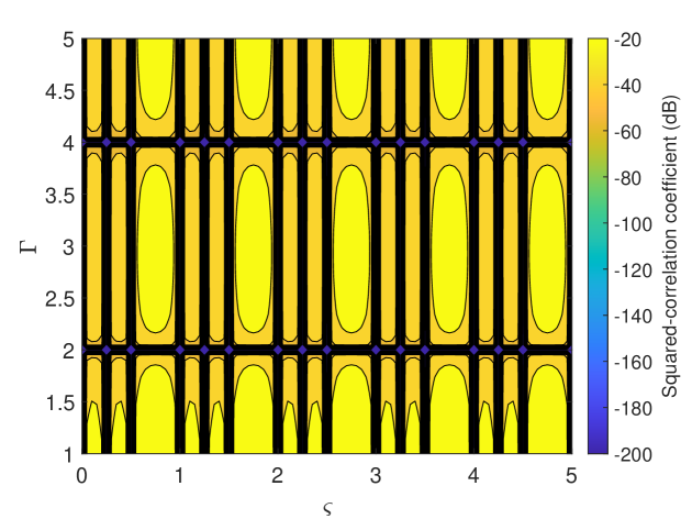
Figure 2: The channels’ squared-correlation coefficient ${\xi_{\lx@text@underscore}{1,2}}$ versus $\varsigma$ and $\Gamma$.

Fig. 2 shows the channels’ squared-correlation coefficient ${\xi_{\lx@text@underscore}{1,2}}$ versus $\varsigma$ and $\Gamma$ for the two-UE communication, by considering the placement positions given in (20) and (21). The UE directions are $\left({{\theta_{\lx@text@underscore}1},{\phi_{\lx@text@underscore}1}}\right)=\left({{{60}^{\circ}},{{30}^{\circ}}}\right)$ and $\left({{\theta_{\lx@text@underscore}2},{\phi_{\lx@text@underscore}2}}\right)=\left({{{30}^{\circ}},{{0}^{\circ}}}\right)$, respectively. The number of UAVs is $L=4$, and each UAV is equipped with a USA with $M=4$ antennas. For convenience of presentation, the coefficient ${\xi_{\lx@text@underscore}{1,2}}$ below $-200$ dB is truncated to $-200$ dB. It is observed that when $\varsigma$ satisfies (54) in Appendix A, the coefficient ${\xi_{\lx@text@underscore}{1,2}}$ is equal to zero, i.e., the channel of UE 1 is orthogonal to that of UE 2, and an IUI-free communication can be obtained. It is also observed that the coefficient ${\xi_{\lx@text@underscore}{1,2}}$ can be reduced by adjusting the sparsity level $\Gamma$, and thus providing an extra DoF for IUI mitigation as compared to the single-antenna UAV.

IV-B Arbitrary Number of UEs

Furthermore, for arbitrary number of UEs, an alternating optimization algorithm similar to Algorithm 1 is proposed, where the receive beamforming, UAV swarm placement positions, and local positions of MAs are alternately optimized in an iterative manner.

IV-B1 Optimization of ${\bf V}$ With Given ${\bf Q}$ and ${\bf B}$

The optimization of receive beamforming is the same as (25), which are omitted for brevity.

IV-B2 Optimization of ${{\bf{q}}_{\lx@text@underscore}l}$ With Given ${\bf V}$, $\left\{{{\bf{q}}_{\lx@text@underscore}{l^{\prime}},\forall l^{\prime}\neq l}\right\}$, and $\bf B$

Let ${{{\bf{\tilde{h}}}}_{\lx@text@underscore}{i,l}}\in{{\mathbb{C}}^{\left({L-1}\right)M\times 1}}$ denote the resulting channel after removing ${{\bf{h}}_{\lx@text@underscore}{i,l}}\in{{\mathbb{C}}^{M\times 1}}={\alpha_{\lx@text@underscore}i}{{\bf{a}}_{\lx@text@underscore}{i,l}}$ from ${{\bf{h}}_{\lx@text@underscore}i}$, ${{{\bf{\tilde{v}}}}_{\lx@text@underscore}{k,l}}\in{{\mathbb{C}}^{\left({L-1}\right)M\times 1}}$ denote the resulting beamforming after removing ${{\bf{v}}_{\lx@text@underscore}{k,l}}\in{\mathbb{C}}^{M\times 1}$ from ${{\bf{v}}_{\lx@text@underscore}k}$, where ${{\bf{h}}_{\lx@text@underscore}{i,l}}$ and ${{\bf{v}}_{\lx@text@underscore}{k,l}}$ denote the $l$-th block of ${{\bf{h}}_{\lx@text@underscore}i}$ and ${{\bf{v}}_{\lx@text@underscore}k}$, respectively. For the case of multi-antenna UAV, after some manipulations, ${f_{\lx@text@underscore}{k,i}}={\left|{{\bf{v}}_{\lx@text@underscore}k^{H}{{\bf{h}}_{\lx@text@underscore}i}}\right|^{2}}$ can be expressed as

$${f_{\lx@text@underscore}{k,i}} =\underbrace{\sum\limits_{\lx@text@underscore}{l^{\prime}=1,l^{\prime}\neq l}^{L}{2{{\left|{{\alpha_{\lx@text@underscore}i}}\right|}^{2}}{\rm{Re}}\left\{{{e^{-{\rm{j}}\frac{{2\pi}}{\lambda}{\bm{\kappa}}_{\lx@text@underscore}i^{T}\left({{{\bf{q}}_{\lx@text@underscore}l}-{{\bf{q}}_{\lx@text@underscore}{l^{\prime}}}}\right)}}{\bf{d}}_{\lx@text@underscore}{i,l}^{H}{{\bf{V}}_{\lx@text@underscore}{k,l,l^{\prime}}}{{\bf{d}}_{\lx@text@underscore}{i,l^{\prime}}}}\right\}}}_{\lx@text@underscore}{{{\tilde{g}}_{\lx@text@underscore}{k,i,l}}}$$ (48)

$$+\underbrace{{{\left|{{\alpha_{\lx@text@underscore}i}}\right|}^{2}}{\bf{d}}_{\lx@text@underscore}{i,l}^{H}{{\bf{V}}_{\lx@text@underscore}{k,l,l}}{{\bf{d}}_{\lx@text@underscore}{i,l}}+{\bf{\tilde{h}}}_{\lx@text@underscore}{i,l}^{H}{{{\bf{\tilde{V}}}}_{\lx@text@underscore}{k,l,l}}{{{\bf{\tilde{h}}}}_{\lx@text@underscore}{i,l}}}_{\lx@text@underscore}{{{\hat{g}}_{\lx@text@underscore}{k,i,l}}},$$

where ${{\bf{d}}_{\lx@text@underscore}{i,l}}\in{{\mathbb{C}}^{M\times 1}}\triangleq{[{e^{{\rm{j}}\frac{{2\pi}}{\lambda}{\bm{\kappa}}_{\lx@text@underscore}i^{T}\left({{{\bf{b}}_{\lx@text@underscore}{l,1}}-{{\bf{q}}_{\lx@text@underscore}r}}\right)}},\cdots,}$ ${{e^{{\rm{j}}\frac{{2\pi}}{\lambda}{\bm{\kappa}}_{\lx@text@underscore}i^{T}\left({{{\bf{b}}_{\lx@text@underscore}{l,M}}-{{\bf{q}}_{\lx@text@underscore}r}}\right)}}]^{T}}$, ${{\bf{V}}_{\lx@text@underscore}{k,l,l^{\prime}}}\in{{\mathbb{C}}^{M\times M}}\triangleq{{\bf{v}}_{\lx@text@underscore}{k,l}}{\bf{v}}_{\lx@text@underscore}{k,l^{\prime}}^{H}$, and ${{{\bf{\tilde{V}}}}_{\lx@text@underscore}{k,l,l}}\in{{\mathbb{C}}^{\left({L-1}\right)M\times\left({L-1}\right)M}}\triangleq{{{\bf{\tilde{v}}}}_{\lx@text@underscore}{k,l}}{\bf{\tilde{v}}}_{\lx@text@underscore}{k,l}^{H}$. Moreover, ${{{\hat{g}}_{\lx@text@underscore}{k,i,l}}}$ is a constant term, and ${{{\tilde{g}}_{\lx@text@underscore}{k,i,l}}}$ can be expressed in terms of ${{{\bf{q}}_{\lx@text@underscore}l}}$ as

$${{\tilde{g}}_{\lx@text@underscore}{k,i,l}} =\sum\limits_{\lx@text@underscore}{l^{\prime}=1,l^{\prime}\neq l}^{L}{2{{\left|{{\alpha_{\lx@text@underscore}i}}\right|}^{2}}\left|{{\bf{d}}_{\lx@text@underscore}{i,l}^{H}{{\bf{V}}_{\lx@text@underscore}{k,l,l^{\prime}}}{{\bf{d}}_{\lx@text@underscore}{i,l^{\prime}}}}\right|\times}$$ (49)

$$\ \ {\rm{cos}}\left({\frac{{2\pi}}{\lambda}{\bm{\kappa}}_{\lx@text@underscore}i^{T}\left({{{\bf{q}}_{\lx@text@underscore}l}-{{\bf{q}}_{\lx@text@underscore}{l^{\prime}}}}\right)-\angle{\bf{d}}_{\lx@text@underscore}{i,l}^{H}{{\bf{V}}_{\lx@text@underscore}{k,l,l^{\prime}}}{{\bf{d}}_{\lx@text@underscore}{i,l^{\prime}}}}\right).$$

A closer look at (49) shows that it has a similar form to (32), and its lower and upper bounds can be correspondingly obtained. As a result, the optimization of ${\bf{q}}_{\lx@text@underscore}l$ for the multi-antenna UAV can follow the similar procedure as in (39).

IV-B3 Optimization of ${b_{\lx@text@underscore}{l,m}}$ With Given ${\bf V}$, ${\bf Q}$, and $\left\{{{b_{\lx@text@underscore}{l^{\prime},m^{\prime}}},\forall l^{\prime}\neq l,m^{\prime}\neq m}\right\}$

The sub-problem of (P1) for optimizing ${b_{\lx@text@underscore}{l,m}}$ is

$$\mathop{\max}\limits_{\lx@text@underscore}{{b_{\lx@text@underscore}{l,m}}} \ \mathop{\min}\limits_{\lx@text@underscore}{k\in{\cal K}}\ {{R_{\lx@text@underscore}k}}$$ (50)

$${\rm{s.t.}} \ {b_{\lx@text@underscore}{l,m}}\in{\tilde{\cal C}},$$

$$\ {\left|{{b_{\lx@text@underscore}{l,m}}-{b_{\lx@text@underscore}{l,m^{\prime}}}}\right|^{2}}\geq\tilde{d}_{\lx@text@underscore}{\min}^{2},\ \forall m^{\prime}\neq m.$$

By following the similar procedure as in Section III-B2, problem (50) can be transformed to

$$\mathop{\max}\limits_{\lx@text@underscore}{{b_{\lx@text@underscore}{l,m}},\rho,\left\{{{\eta_{\lx@text@underscore}k},{\mu_{\lx@text@underscore}k}}\right\}_{\lx@text@underscore}{k=1}^{K}}\ \ \rho$$ (51)

$${\rm{s.t.}} \ {{{\eta_{\lx@text@underscore}k}-{\mu_{\lx@text@underscore}k}}}\geq\rho\ln 2,\ \forall k\in{\cal K},$$

$${\sigma^{2}}+\sum\limits_{\lx@text@underscore}{i=1}^{K}{{P_{\lx@text@underscore}i}{{\left|{{\bf{v}}_{\lx@text@underscore}k^{H}{{\bf{h}}_{\lx@text@underscore}i}}\right|}^{2}}}\geq{\sigma^{2}}{e^{{\eta_{\lx@text@underscore}k}}},\ \forall k\in{\cal K},$$

$${\sigma^{2}}+\sum\limits_{\lx@text@underscore}{i=1,i\neq k}^{K}{{P_{\lx@text@underscore}i}{{\left|{{\bf{v}}_{\lx@text@underscore}k^{H}{{\bf{h}}_{\lx@text@underscore}i}}\right|}^{2}}}\leq{\sigma^{2}}{e^{{\mu_{\lx@text@underscore}k}}},\ \forall k\in{\cal K},$$

$${b_{\lx@text@underscore}{l,m}}\in{\tilde{\cal C}},$$

$${\left|{{b_{\lx@text@underscore}{l,m}}-{b_{\lx@text@underscore}{l,m^{\prime}}}}\right|^{2}}\geq\tilde{d}_{\lx@text@underscore}{\min}^{2},\ \forall m^{\prime}\neq m.$$

Let ${{\bf{\tilde{h}}}_{\lx@text@underscore}{i,l,m}}\in{{\mathbb{C}}^{\left({LM-1}\right)\times 1}}$ and ${{\bf{\tilde{v}}}_{\lx@text@underscore}{i,l,m}}\in{{\mathbb{C}}^{\left({LM-1}\right)\times 1}}$ denote the resulting channel and beamforming vector after removing ${h_{\lx@text@underscore}{i,l,m}}$ and ${v_{\lx@text@underscore}{i,l,m}}$, respectively, where ${h_{\lx@text@underscore}{i,l,m}}$ and ${v_{\lx@text@underscore}{i,l,m}}$ are the $\left({\left({l-1}\right)M+m}\right)$-th elements of ${{{\bf{h}}_{\lx@text@underscore}i}}$ and ${{{\bf{v}}_{\lx@text@underscore}k}}$, respectively. The expression ${f_{\lx@text@underscore}{k,i}}={\left|{{\bf{v}}_{\lx@text@underscore}k^{H}{{\bf{h}}_{\lx@text@underscore}i}}\right|^{2}}$ can be expressed as

$${f_{\lx@text@underscore}{k,i}}=\underbrace{2\left|{{c_{\lx@text@underscore}{k,i,l,m}}}\right|{\mathop{\rm Re}\nolimits}\left\{{{e^{{\rm{j}}\left({\frac{{2\pi}}{\lambda}{\Phi_{\lx@text@underscore}i}{b_{\lx@text@underscore}{l,m}}+\angle{c_{\lx@text@underscore}{k,i,l,m}}}\right)}}}\right\}}_{\lx@text@underscore}{{g_{\lx@text@underscore}{k,i,l,m}}}+$$ (52)

$$\underbrace{{{\left|{{\alpha_{\lx@text@underscore}i}}\right|}^{2}}{{\left|{{v_{\lx@text@underscore}{k,l,m}}}\right|}^{2}}+{\bf{\tilde{h}}}_{\lx@text@underscore}{i,l,m}^{H}{{{\bf{\tilde{v}}}}_{\lx@text@underscore}{k,l,m}}{\bf{\tilde{v}}}_{\lx@text@underscore}{k,l,m}^{H}{{{\bf{\tilde{h}}}}_{\lx@text@underscore}{i,l,m}}}_{\lx@text@underscore}{{{\bar{g}}_{\lx@text@underscore}{k,i,l,m}}},$$

where ${c_{\lx@text@underscore}{k,i,l,m}}\triangleq{\bf{\tilde{h}}}_{\lx@text@underscore}{i,l,m}^{H}{{{\bf{\tilde{v}}}}_{\lx@text@underscore}{k,l,m}}v_{\lx@text@underscore}{k,l,m}^{*}{\alpha_{\lx@text@underscore}i}\times$ ${e^{{\rm{j}}\frac{{2\pi}}{\lambda}{\bm{\kappa}}_{\lx@text@underscore}i^{T}\left({{{\bf{q}}_{\lx@text@underscore}l}-{{\bf{q}}_{\lx@text@underscore}r}}\right)}}$, and ${{{\bar{g}}_{\lx@text@underscore}{k,i,l,m}}}$ is independent of ${{b_{\lx@text@underscore}{l,m}}}$. Thus, problem (51) can be solved similar to (30).

The main procedures for solving problem (P1) are summarized in Algorithm 2. The complexity for obtaining the receive beamforming in step 3 is ${\cal O}({K{(LM)^{3}}})$. From step 4 to step 6, the complexity is approximately ${\cal O}({I_{\lx@text@underscore}1}L{{({2K})}^{3}})$, where $I_{\lx@text@underscore}1$ denotes the maximum number of iterations required by SCA for convergence. The complexity from step 7 to step 11 is approximately given by ${\cal O}({I_{\lx@text@underscore}2}L(M-1){{({2K})}^{3}})$, where $I_{\lx@text@underscore}2$ denotes the maximum number of iterations to converge required by step 9. As a result, the total computational complexity of Algorithm 2 is ${\cal O}({{I_{\lx@text@underscore}3}K{(LM)^{3}}+{I_{\lx@text@underscore}2}{I_{\lx@text@underscore}3}L(M-1){({2K})}^{3}})$, where $I_{\lx@text@underscore}3$ denotes the number of iterations required by the alternating optimization for convergence.

Algorithm 2 Proposed Alternating Optimization for Solving Problem (P1)

1: Initialize ${{\bf{Q}}^{\left(j\right)}}$, ${{\bf{B}}^{\left(j\right)}}$, and $\{{{\bf{v}}_{\lx@text@underscore}k^{\left(j\right)}}\}$ randomly, and let $j=0$.

2: repeat

3:  For given ${{\bf{Q}}^{\left(j\right)}}$ and ${{\bf{B}}^{\left(j\right)}}$, obtain the optimal beamforming $\{{{\bf{v}}_{\lx@text@underscore}k^{\left({j+1}\right)}}\}$.

4:  for $l=1:L$ do

5:   Obtain $\{{\bf{q}}_{\lx@text@underscore}l^{\left({j+1}\right)}\}$ similar to problem (39), given  $\{{\bf{q}}_{\lx@text@underscore}1^{\left({j+1}\right)},\cdots,{\bf{q}}_{\lx@text@underscore}{l-1}^{\left({j+1}\right)},{\bf{q}}_{\lx@text@underscore}{l+1}^{\left(j\right)},\cdots,{\bf{q}}_{\lx@text@underscore}L^{\left(j\right)}\}$, ${{\bf{B}}^{\left(j\right)}}$,  and $\{{{\bf{v}}_{\lx@text@underscore}k^{\left({j+1}\right)}}\}$.

6:  end for

7:  for $l=1:L$ do

8:   for $m=2:M$ do

9:    Obtain ${b_{\lx@text@underscore}{l,m}^{\left({j+1}\right)}}$ given ${{\bf{Q}}^{\left({j+1}\right)}}$, $\{b_{\lx@text@underscore}{1,2}^{\left({j+1}\right)},\cdots,$  $b_{\lx@text@underscore}{l,m-1}^{\left({j+1}\right)},b_{\lx@text@underscore}{l,m+1}^{\left(j\right)},\cdots b_{\lx@text@underscore}{L,M}^{\left(j\right)}\}$, and $\{{{\bf{v}}_{\lx@text@underscore}k^{\left({j+1}\right)}}\}$.

10:   end for

11:  end for

12:  Update $j=j+1$.

13: until the fractional increase in the objective function value is below a given threshold $\epsilon>0$.

V Numerical Results

In this section, numerical results are provided to verify the performance of the proposed low-altitude UAV swarm enabled MA system. The channel power at the reference distance of ${d_{\lx@text@underscore}0}=1$ m is ${\beta_{\lx@text@underscore}0}=-61.4$ dB, and the noise power is ${\sigma^{2}}=-94$ dBm. The minimum distance to avoid the collision among UAVs is ${d_{\lx@text@underscore}{\min}}=1$ m. The movable region of UAVs is specified by ${x_{\lx@text@underscore}l}\in\left[{-30,30}\right]$ m, ${y_{\lx@text@underscore}l}\in\left[{-30,30}\right]$ m, and ${z_{\lx@text@underscore}l}\in\left[{85,115}\right]$ m. Moreover, the minimum distance to avoid mutual coupling between adjacent MA elements is ${{\tilde{d}}_{\lx@text@underscore}{\min}}=\lambda/2$. The (local) movable region of MAs at each UAV is $\left[{0,D}\right]$, with $D=20\lambda$. Unless otherwise stated, $K=3$ UEs are uniformly distributed in a circular area with the center and radius being $\left[{0,0,0}\right]^{T}$ m and $200$ m, respectively. The transmit power of each UE is $P_{\lx@text@underscore}k=10$ dBm.

V-A Single-Antenna UAV

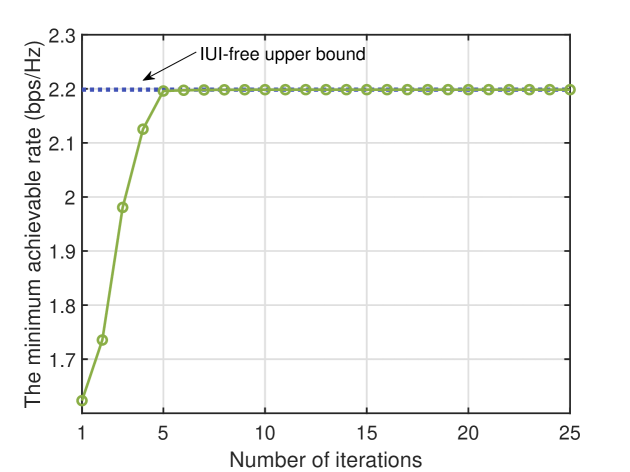
Figure 3: Convergence behaviour of Algorithm 1.

First, we consider the case of single-antenna UAVs, with $L=4$. Fig. 3 shows the convergence behaviour of Algorithm 1. The upper bound of IUI-free communication is also provided for comparison, i.e., the result given in (22). It is observed that Algorithm 1 yields a non-decreasing minimum achievable rate, and finally approaches the converged solution that is close to the IUI-free upper bound.

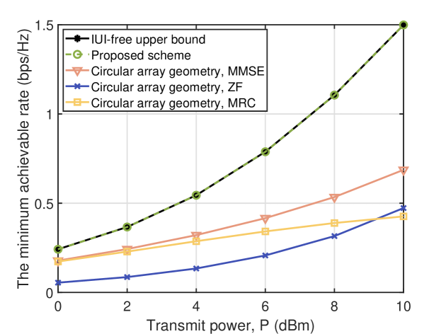
Figure 4: The minimum achievable rate versus the transmit power of each UE for the two-UE communication in the single-antenna UAV case.

Fig. 4 shows the minimum achievable rate versus the transmit power of each UE for the two-UE communication, by considering the UE directions $\left({{\theta_{\lx@text@underscore}1},{\phi_{\lx@text@underscore}1}}\right)=\left({{{60}^{\circ}},{{30}^{\circ}}}\right)$ and $\left({{\theta_{\lx@text@underscore}2},{\phi_{\lx@text@underscore}2}}\right)=\left({{{30}^{\circ}},{{0}^{\circ}}}\right)$, respectively. For comparison, the benchmark scheme of circular array geometry is considered, i.e., the UAV swarm cooperatively forms a circular array, with their placement positions given by

$${{\bf{q}}_{\lx@text@underscore}l}{\rm=}{{\bf{q}}_{\lx@text@underscore}r}+\left[R\cos\left({\frac{{2\pi}}{L}\left({l-1}\right)}\right),{R\sin\left({\frac{{2\pi}}{L}\left({l-1}\right)}\right),0}\right]^{T},\ \forall l,$$ (53)

where $R$ denotes the radius of circular array geometry and is set as $R=7.5$ m. With the circular array geometry, the MMSE, ZF and MRC beamforming schemes are respectively considered. It is observed that the proposed UAV swarm enabled MA system achieves an IUI-free communication, thanks to the flexible placement position optimization. Besides, the proposed scheme significantly outperforms the benchmark schemes of circular array geometry with MMSE, ZF, and MRC beamforming. This is expected since the proposed scheme is able to completely orthogonalize the channels of two UEs, while achieving the full beamforming gain at each UE. Specifically, Fig. 5 shows the SNR loss factor versus the transmit power for UE 1. It is observed that the proposed scheme always enjoys a zero SNR loss factor. By contrast, the circular array geometry with MMSE and MRC beamforming schemes experience increased SNR loss factors as the transmit power increases, as a result of suffering from more severe IUI, especially for the MRC beamforming scheme.

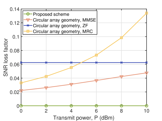
Figure 5: The SNR loss factor versus the transmit power for the two-UE communication in the single-antenna UAV case.

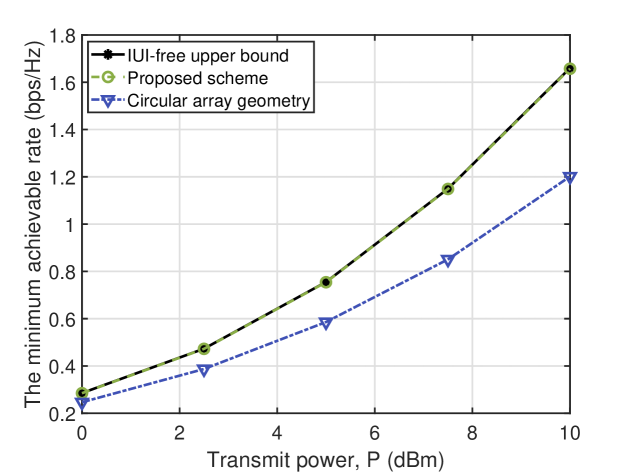
Figure 6: The minimum achievable rate versus the transmit power of each UE for three UEs in the single-antenna UAV case.

For further comparison, Fig. 6 shows the minimum achievable rate versus the transmit power of each UE for $K=3$ UEs. Since MMSE beamforming achieves the balance between reducing the interference and noise enhancement, the benchmark scheme of circular array geometry with MMSE beamforming is considered in the following. It is observed that the minimum achievable rate of both the proposed and benchmark schemes increase as the transmit power increases, as expected. Besides, similar to the case of two UEs, the proposed UAV swarm enabled MA system yields a comparable performance to the IUI-free upper bound, and is significantly superior to the benchmark scheme of circular array geometry with MMSE beamforming. This is expected since the proposed scheme can strike an optimal balance between the beamforming gain improvement and IUI mitigation via the flexible UAV placement position adjustment.

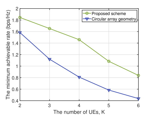
Figure 7: The minimum achievable rate versus the number of UEs in the single-antenna UAV case.

Fig. 7 shows the minimum achievable rate versus the number of UEs, $K$. It is observed that the performance of both schemes decrease as the number of UEs increases. This is because more UEs will cause a severer IUI issue, especially when the number of UAVs/antennas is smaller than that of UEs. It is also observed that the minimum achievable rate of the proposed UAV swarm enabled MA system always surpasses the benchmark scheme of circular array geometry, thanks to the flexible UAV placement position adjustment to significantly reduce the channel correlation and thus the IUI among UEs.

V-B Multi-Antenna UAV

Next, we consider the case of multi-antenna UAVs, where the numbers of UAVs and MAs per UAV are $L=2$ and $M=4$, respectively. For comparison, the following two benchmark schemes are considered: 1) Circular array geometry with FPA: each UAV is equipped with an FPA array (linear) and UAV swarm adopts the circular geometry given in (53); 2) Placement optimization with FPA: each UAV is equipped with the FPA array as above and UAV swarm placement is optimized similar to Section IV-B. Fig. 8 shows the minimum achievable rate versus the transmit power of each UE for the case with $K=3$ UEs. It is observed that the performance of UAV swarm enabled MA system is very close to that of the IUI-free communication, and its performance gains over the other two benchmark schemes become even more significant as the transmit power increases. This is due to the two-level mobility brought by UAV swarm enabled MA system, i.e., the intrinsic mobility of UAV swarm and additional antenna position adjustment of MA. Specifically, it can be observed that the scheme of placement optimization with FPA yields a better performance than that of circular UAV geometry with FPA, which demonstrates the importance of UAV swarm placement optimization for performance improvement. Moreover, compared to the scheme of placement optimization with FPA, considerable performance gain is achieved for UAV swarm enabled MA system, thanks to the additional antenna position adjustment of MA. The above results verify the advantages of two-level mobility brought by UAV swarm enabled MA system, i.e., it can fully exploit channel variation for balancing the beamforming gain improvement and IUI reduction.

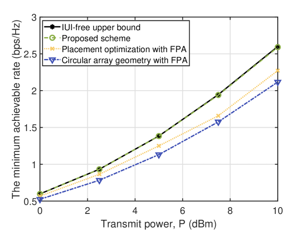
Figure 8: The minimum achievable rate versus the transmit power of each UE in the multi-antenna UAV case.

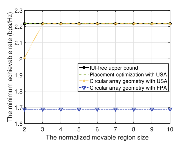
(a) $K=2$

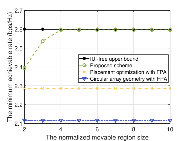
(b) $K=3$

Figure 9: The minimum achievable rate versus the normalized movable region size in the multi-antenna UAV case.

Last, Fig. 9 studies the impact of the normalized movable region size $D/\lambda$ on the minimum achievable rate. For $K=2$, the UE directions are the same as for Fig. 4, and the following three schemes are considered: 1) Placement optimization with USA: each UAV is equipped with a USA and UAV swarm adopts the placement given in (20) and (21); 2) Circular array geometry with USA: each UAV is equipped with a USA and UAV swarm adopts the circular geometry given in (53); 3) Circular array geometry with FPA: Similar to 2), but using FPA instead USA. For USA, the sparsity level can be dynamically adjusted. It is firstly observed from Fig. 9(a) that the scheme of placement optimization with USA directly achieves the IUI-free communication. This is because the placement given in (20) and (21) orthogonalizes the channels of two UEs. On the other hand, as the normalized movable region size increases, the scheme of circular array geometry with USA also achieves the IUI-free communication, thanks to the extra DoF of sparsity level adjustment for completely eliminating the IUI. Moreover, for $K=3$, it is observed from Fig. 9(b) that the performance of two FPA schemes remain unchanged as the normalized movable region size increases, as expected. By contrast, the performance of the proposed UAV swarm enabled MA system first increases and ultimately converges as the normalized movable region size increases. This is mainly attributed to the fact that with an enlarged movable region size, MA array has a larger spatial DoF to create favorable channels for performance improvement. However, this does not mean that the performance gain of UAV swarm enabled MA system over other benchmark schemes will continuously increase, since it is bounded by the IUI-free communication from above.

VI Conclusion

This paper proposed a novel UAV swarm enabled two-level MA system to support low-altitude economy, by exploiting the controllable mobility of UAV and antenna position adjustment of MA. An optimization problem was formulated to maximize the minimum achievable rate over all ground UEs, by jointly optimizing 3D UAV swarm placement positions, their individual MAs’ positions, and receive beamforming for UEs. To gain useful insights, we first considered the special case of single-antenna UAV. It was shown that the resulting SNR of single UE communication is independent of UAV swarm array geometry, and the optimal UAV swarm placement positions were derived in closed-form for two-UE communication. For arbitrary number of UEs, an alternating optimization algorithm was proposed to efficiently solve the formulated non-convex problem. Moreover, the results of single-antenna UAV were extended to the general case with multi-antenna UAV. Numerical results demonstrated that significant performance gains can be achieved for the proposed UAV swarm enabled MA system over various benchmarks, thanks to the two-level antenna mobility to create more favorable channels.

Appendix A Proof of Theorem 1

By substituting ${{\bf{q}}_{\lx@text@underscore}l}={{\bf{q}}_{\lx@text@underscore}1}+\left({l-1}\right)\times$ $\frac{{\left({{\varsigma}+1/L}\right)\lambda}}{{{{\left\|{{{\bm{\kappa}}_{\lx@text@underscore}k}-{{\bm{\kappa}}_{\lx@text@underscore}{k^{\prime}}}}\right\|}^{2}}}}\left({{{\bm{\kappa}}_{\lx@text@underscore}k}-{{\bm{\kappa}}_{\lx@text@underscore}{k^{\prime}}}}\right)$ into (19), where $\varsigma$ is a common coefficient to all the UAVs, given by

$$\varsigma\in\left\{{\left.{\frac{\nu}{L}}\right|\nu\in{\mathbb{Z}},\bmod\left({\nu+1,L}\right)\neq 0}\right\},$$ (54)

it can be verified that the objective value of (19) is equal to zero. Moreover, the distance between UAV $l$ and $l^{\prime}$ is given by

$$\left\|{{{\bf{q}}_{\lx@text@underscore}l}-{{\bf{q}}_{\lx@text@underscore}{l^{\prime}}}}\right\|=\left\|{\left({l-l^{\prime}}\right)\left({\varsigma+1/L}\right)\lambda\frac{{\left({{{\bm{\kappa}}_{\lx@text@underscore}k}-{{\bm{\kappa}}_{\lx@text@underscore}{k^{\prime}}}}\right)}}{{{{\left\|{{{\bm{\kappa}}_{\lx@text@underscore}k}-{{\bm{\kappa}}_{\lx@text@underscore}{k^{\prime}}}}\right\|}^{2}}}}}\right\|$$ (55)

$$\geq\left\|{\left({\varsigma+1/L}\right)\lambda\frac{{\left({{{\bm{\kappa}}_{\lx@text@underscore}k}-{{\bm{\kappa}}_{\lx@text@underscore}{k^{\prime}}}}\right)}}{{{{\left\|{{{\bm{\kappa}}_{\lx@text@underscore}k}-{{\bm{\kappa}}_{\lx@text@underscore}{k^{\prime}}}}\right\|}^{2}}}}}\right\|=\frac{{\lambda\left|{\varsigma+1/L}\right|}}{{\left\|{{{\bm{\kappa}}_{\lx@text@underscore}k}-{{\bm{\kappa}}_{\lx@text@underscore}{k^{\prime}}}}\right\|}}.$$

To satisfy the collision avoidance constraint for UAVs, a feasible solution of $\varsigma$ is thus given by (21). This completes the proof of Theorem 1.

Appendix B Proof of Lemma 1

With ${g_{\lx@text@underscore}{k,i,l}}$ given in (32), its lower and upper bounds can be constructed based on the second-order Taylor expansion [47, 24, 48]. Specifically, the gradient of ${g_{\lx@text@underscore}{k,i,l}}$ over ${{{\bf{q}}_{\lx@text@underscore}l}}$ is $\nabla{g_{\lx@text@underscore}{k,i,l}}={\left[{\frac{{\partial{g_{\lx@text@underscore}{k,i,l}}}}{{\partial{x_{\lx@text@underscore}l}}},\frac{{\partial{g_{\lx@text@underscore}{k,i,l}}}}{{\partial{y_{\lx@text@underscore}l}}},\frac{{\partial{g_{\lx@text@underscore}{k,i,l}}}}{{\partial{z_{\lx@text@underscore}l}}}}\right]^{T}}$, where

$$\frac{{\partial{g_{\lx@text@underscore}{k,i,l}}}}{{\partial{x_{\lx@text@underscore}l}}}=-\frac{{2\pi}}{\lambda}\sum\limits_{\lx@text@underscore}{l^{\prime}=1,l^{\prime}\neq l}^{L}{2{{\left|{{\alpha_{\lx@text@underscore}i}}\right|}^{2}}\left|{{V_{\lx@text@underscore}{k,l,l^{\prime}}}}\right|}{\Phi_{\lx@text@underscore}i}$$ (56)

$$\ \ \ \ \ \ \ \ \ \ \times\sin\left({\frac{{2\pi}}{\lambda}{\bm{\kappa}}_{\lx@text@underscore}i^{T}\left({{{\bf{q}}_{\lx@text@underscore}l}-{{\bf{q}}_{\lx@text@underscore}{l^{\prime}}}}\right)-\angle{V_{\lx@text@underscore}{k,l,l^{\prime}}}}\right),$$

$$\frac{{\partial{g_{\lx@text@underscore}{k,i,l}}}}{{\partial{y_{\lx@text@underscore}l}}}=-\frac{{2\pi}}{\lambda}\sum\limits_{\lx@text@underscore}{l^{\prime}=1,l^{\prime}\neq l}^{L}{2{{\left|{{\alpha_{\lx@text@underscore}i}}\right|}^{2}}\left|{{V_{\lx@text@underscore}{k,l,l^{\prime}}}}\right|}{\Psi_{\lx@text@underscore}i}$$ (57)

$$\ \ \ \ \ \ \ \ \ \ \times\sin\left({\frac{{2\pi}}{\lambda}{\bm{\kappa}}_{\lx@text@underscore}i^{T}\left({{{\bf{q}}_{\lx@text@underscore}l}-{{\bf{q}}_{\lx@text@underscore}{l^{\prime}}}}\right)-\angle{V_{\lx@text@underscore}{k,l,l^{\prime}}}}\right),$$

$$\frac{{\partial{g_{\lx@text@underscore}{k,i,l}}}}{{\partial{z_{\lx@text@underscore}l}}}=-\frac{{2\pi}}{\lambda}\sum\limits_{\lx@text@underscore}{l^{\prime}=1,l^{\prime}\neq l}^{L}{2{{\left|{{\alpha_{\lx@text@underscore}i}}\right|}^{2}}\left|{{V_{\lx@text@underscore}{k,l,l^{\prime}}}}\right|}{\Theta_{\lx@text@underscore}i}$$ (58)

$$\ \ \ \ \ \ \ \ \ \ \times\sin\left({\frac{{2\pi}}{\lambda}{\bm{\kappa}}_{\lx@text@underscore}i^{T}\left({{{\bf{q}}_{\lx@text@underscore}l}-{{\bf{q}}_{\lx@text@underscore}{l^{\prime}}}}\right)-\angle{V_{\lx@text@underscore}{k,l,l^{\prime}}}}\right),$$

Besides, the Hessian matrix of ${{g_{\lx@text@underscore}{k,i,l}}}$ over ${{{\bf{q}}_{\lx@text@underscore}l}}$ is

$${\nabla^{2}}{g_{\lx@text@underscore}{k,i,l}}{\rm=}\left[{\begin{array}[]{*{20}{c}}{\frac{{{\partial^{2}}{g_{\lx@text@underscore}{k,i,l}}}}{{\partial{x_{\lx@text@underscore}l}\partial{x_{\lx@text@underscore}l}}}}&{\frac{{{\partial^{2}}{g_{\lx@text@underscore}{k,i,l}}}}{{\partial{x_{\lx@text@underscore}l}\partial{y_{\lx@text@underscore}l}}}}&{\frac{{{\partial^{2}}{g_{\lx@text@underscore}{k,i,l}}}}{{\partial{x_{\lx@text@underscore}l}\partial{z_{\lx@text@underscore}l}}}}\\ {\frac{{{\partial^{2}}{g_{\lx@text@underscore}{k,i,l}}}}{{\partial{y_{\lx@text@underscore}l}\partial{x_{\lx@text@underscore}l}}}}&{\frac{{{\partial^{2}}{g_{\lx@text@underscore}{k,i,l}}}}{{\partial{y_{\lx@text@underscore}l}\partial{y_{\lx@text@underscore}l}}}}&{\frac{{{\partial^{2}}{g_{\lx@text@underscore}{k,i,l}}}}{{\partial{y_{\lx@text@underscore}l}\partial{z_{\lx@text@underscore}l}}}}\\ {\frac{{{\partial^{2}}{g_{\lx@text@underscore}{k,i,l}}}}{{\partial{z_{\lx@text@underscore}l}\partial{x_{\lx@text@underscore}l}}}}&{\frac{{{\partial^{2}}{g_{\lx@text@underscore}{k,i,l}}}}{{\partial{z_{\lx@text@underscore}l}\partial{y_{\lx@text@underscore}l}}}}&{\frac{{{\partial^{2}}{g_{\lx@text@underscore}{k,i,l}}}}{{\partial{z_{\lx@text@underscore}l}\partial{z_{\lx@text@underscore}l}}}}\end{array}}\right],$$ (59)

where

$$\frac{{{\partial^{2}}{g_{\lx@text@underscore}{k,i,l}}}}{{\partial{x_{\lx@text@underscore}l}\partial{x_{\lx@text@underscore}l}}}=-{\left({\frac{{2\pi}}{\lambda}}\right)^{2}}\sum\limits_{\lx@text@underscore}{l^{\prime}=1,l^{\prime}\neq l}^{L}{2{{\left|{{\alpha_{\lx@text@underscore}i}}\right|}^{2}}\left|{{V_{\lx@text@underscore}{k,l,l^{\prime}}}}\right|}\Phi_{\lx@text@underscore}i^{2}$$ (60)

$$\times\cos\left({\frac{{2\pi}}{\lambda}{\bm{\kappa}}_{\lx@text@underscore}i^{T}\left({{{\bf{q}}_{\lx@text@underscore}l}-{{\bf{q}}_{\lx@text@underscore}{l^{\prime}}}}\right)-\angle{V_{\lx@text@underscore}{k,l,l^{\prime}}}}\right),$$

$$\frac{{{\partial^{2}}{g_{\lx@text@underscore}{k,i,l}}}}{{\partial{y_{\lx@text@underscore}l}\partial{y_{\lx@text@underscore}l}}}=-{\left({\frac{{2\pi}}{\lambda}}\right)^{2}}\sum\limits_{\lx@text@underscore}{l^{\prime}=1,l^{\prime}\neq l}^{L}{2{{\left|{{\alpha_{\lx@text@underscore}i}}\right|}^{2}}\left|{{V_{\lx@text@underscore}{k,l,l^{\prime}}}}\right|}\Psi_{\lx@text@underscore}i^{2}$$ (61)

$$\times\cos\left({\frac{{2\pi}}{\lambda}{\bm{\kappa}}_{\lx@text@underscore}i^{T}\left({{{\bf{q}}_{\lx@text@underscore}l}-{{\bf{q}}_{\lx@text@underscore}{l^{\prime}}}}\right)-\angle{V_{\lx@text@underscore}{k,l,l^{\prime}}}}\right),$$

$$\frac{{{\partial^{2}}{g_{\lx@text@underscore}{k,i,l}}}}{{\partial{z_{\lx@text@underscore}l}\partial{z_{\lx@text@underscore}l}}}=-{\left({\frac{{2\pi}}{\lambda}}\right)^{2}}\sum\limits_{\lx@text@underscore}{l^{\prime}=1,l^{\prime}\neq l}^{L}{2{{\left|{{\alpha_{\lx@text@underscore}i}}\right|}^{2}}\left|{{V_{\lx@text@underscore}{k,l,l^{\prime}}}}\right|}\Theta_{\lx@text@underscore}i^{2}$$ (62)

$$\times\cos\left({\frac{{2\pi}}{\lambda}{\bm{\kappa}}_{\lx@text@underscore}i^{T}\left({{{\bf{q}}_{\lx@text@underscore}l}-{{\bf{q}}_{\lx@text@underscore}{l^{\prime}}}}\right)-\angle{V_{\lx@text@underscore}{k,l,l^{\prime}}}}\right),$$

$$\frac{{{\partial^{2}}{g_{\lx@text@underscore}{k,i,l}}}}{{\partial{x_{\lx@text@underscore}l}\partial{y_{\lx@text@underscore}l}}} =\frac{{{\partial^{2}}{g_{\lx@text@underscore}{k,i,l}}}}{{\partial{y_{\lx@text@underscore}l}\partial{x_{\lx@text@underscore}l}}}=-{\left({\frac{{2\pi}}{\lambda}}\right)^{2}}\sum\limits_{\lx@text@underscore}{l^{\prime}=1,l^{\prime}\neq l}^{L}{2{{\left|{{\alpha_{\lx@text@underscore}i}}\right|}^{2}}\left|{{V_{\lx@text@underscore}{k,l,l^{\prime}}}}\right|{\Phi_{\lx@text@underscore}i}{\Psi_{\lx@text@underscore}i}}$$ (63)

$$\ \ \ \ \ \times\cos\left({\frac{{2\pi}}{\lambda}{\bm{\kappa}}_{\lx@text@underscore}i^{T}\left({{{\bf{q}}_{\lx@text@underscore}l}-{{\bf{q}}_{\lx@text@underscore}{l^{\prime}}}}\right)-\angle{V_{\lx@text@underscore}{k,l,l^{\prime}}}}\right),$$

$$\frac{{{\partial^{2}}{g_{\lx@text@underscore}{k,i,l}}}}{{\partial{x_{\lx@text@underscore}l}\partial{z_{\lx@text@underscore}l}}} =\frac{{{\partial^{2}}{g_{\lx@text@underscore}{k,i,l}}}}{{\partial{z_{\lx@text@underscore}l}\partial{x_{\lx@text@underscore}l}}}=-{\left({\frac{{2\pi}}{\lambda}}\right)^{2}}\sum\limits_{\lx@text@underscore}{l^{\prime}=1,l^{\prime}\neq l}^{L}{2{{\left|{{\alpha_{\lx@text@underscore}i}}\right|}^{2}}\left|{{V_{\lx@text@underscore}{k,l,l^{\prime}}}}\right|{\Phi_{\lx@text@underscore}i}{\Theta_{\lx@text@underscore}i}}$$ (64)

$$\ \ \ \ \ \times\cos\left({\frac{{2\pi}}{\lambda}{\bm{\kappa}}_{\lx@text@underscore}i^{T}\left({{{\bf{q}}_{\lx@text@underscore}l}-{{\bf{q}}_{\lx@text@underscore}{l^{\prime}}}}\right)-\angle{V_{\lx@text@underscore}{k,l,l^{\prime}}}}\right),$$

$$\frac{{{\partial^{2}}{g_{\lx@text@underscore}{k,i,l}}}}{{\partial{y_{\lx@text@underscore}l}\partial{z_{\lx@text@underscore}l}}} =\frac{{{\partial^{2}}{g_{\lx@text@underscore}{k,i,l}}}}{{\partial{z_{\lx@text@underscore}l}\partial{y_{\lx@text@underscore}l}}}=-{\left({\frac{{2\pi}}{\lambda}}\right)^{2}}\sum\limits_{\lx@text@underscore}{l^{\prime}=1,l^{\prime}\neq l}^{L}{2{{\left|{{\alpha_{\lx@text@underscore}i}}\right|}^{2}}\left|{{V_{\lx@text@underscore}{k,l,l^{\prime}}}}\right|{\Psi_{\lx@text@underscore}i}{\Theta_{\lx@text@underscore}i}}$$ (65)

$$\ \ \ \ \ \times\cos\left({\frac{{2\pi}}{\lambda}{\bm{\kappa}}_{\lx@text@underscore}i^{T}\left({{{\bf{q}}_{\lx@text@underscore}l}-{{\bf{q}}_{\lx@text@underscore}{l^{\prime}}}}\right)-\angle{V_{\lx@text@underscore}{k,l,l^{\prime}}}}\right).$$

Moreover, with (59), it follows that

$$\left\|{{\nabla^{2}}{g_{\lx@text@underscore}{k,i,l}}}\right\|_{\lx@text@underscore}2^{2}\leq\left\|{{\nabla^{2}}{g_{\lx@text@underscore}{k,i,l}}}\right\|_{\lx@text@underscore}F^{2}$$ (66)

$$\ \ \ ={\left({\frac{{{\partial^{2}}{g_{\lx@text@underscore}{k,i,l}}}}{{\partial{x_{\lx@text@underscore}l}\partial{x_{\lx@text@underscore}l}}}}\right)^{2}}+\cdots+{\left({\frac{{{\partial^{2}}{g_{\lx@text@underscore}{k,i,l}}}}{{\partial{z_{\lx@text@underscore}l}\partial{z_{\lx@text@underscore}l}}}}\right)^{2}}$$

$$\ \ \ \leq{\left({\frac{{4{\pi^{2}}}}{{{\lambda^{2}}}}\sum\limits_{\lx@text@underscore}{l^{\prime}=1,l^{\prime}\neq l}^{L}{2{{\left|{{\alpha_{\lx@text@underscore}i}}\right|}^{2}}\left|{{V_{\lx@text@underscore}{k,l,l^{\prime}}}}\right|}}\right)^{2}}\left({\Phi_{\lx@text@underscore}i^{4}+\Phi_{\lx@text@underscore}i^{2}\Psi_{\lx@text@underscore}i^{2}+}\right.$$

$$\ \ \ \ \ \ \left.{\Phi_{\lx@text@underscore}i^{2}\Theta_{\lx@text@underscore}i^{2}+\Psi_{\lx@text@underscore}i^{2}\Phi_{\lx@text@underscore}i^{2}+\Psi_{\lx@text@underscore}i^{4}+\Psi_{\lx@text@underscore}i^{2}\Theta_{\lx@text@underscore}i^{2}+\Theta_{\lx@text@underscore}i^{2}\Phi_{\lx@text@underscore}i^{2}+\Theta_{\lx@text@underscore}i^{2}\Psi_{\lx@text@underscore}i^{2}+\Theta_{\lx@text@underscore}i^{4}}\right)$$

$$\ \ \ ={\left({\frac{{4{\pi^{2}}}}{{{\lambda^{2}}}}\sum\limits_{\lx@text@underscore}{l^{\prime}=1,l^{\prime}\neq l}^{L}{2{{\left|{{\alpha_{\lx@text@underscore}i}}\right|}^{2}}\left|{{V_{\lx@text@underscore}{k,l,l^{\prime}}}}\right|}}\right)^{2}}.$$

With ${\nabla^{2}}{g_{\lx@text@underscore}{k,i,l}}\preceq{\left\|{{\nabla^{2}}{g_{\lx@text@underscore}{k,i,l}}}\right\|_{\lx@text@underscore}2}{\bf{I}}$, and by choosing ${\delta_{\lx@text@underscore}{k,i,l}}=\frac{{8{\pi^{2}}}}{{{\lambda^{2}}}}{\left|{{\alpha_{\lx@text@underscore}i}}\right|^{2}}\sum\nolimits_{\lx@text@underscore}{l^{\prime}=1,l^{\prime}\neq l}^{L}{\left|{{V_{\lx@text@underscore}{k,l,l^{\prime}}}}\right|}$, we have ${\nabla^{2}}{g_{\lx@text@underscore}{k,i,l}}\preceq{\delta_{\lx@text@underscore}{k,i,l}}{\bf{I}}$. Thus, the lower and upper bounds of ${{g_{\lx@text@underscore}{k,i,l}}}$ in (33) and (34) can be obtained with the Taylor’s theorem [47]. The proof of Lemma 1 is thus completed.

References

- [1] Y. Jiang, X. Li, G. Zhu, H. Li, J. Deng, K. Han, C. Shen, Q. Shi, and R. Zhang, “6G non-terrestrial networks enabled low-altitude economy: Opportunities and challenges,” arXiv preprint arXiv:2311.09047, 2023.
- [2] G. Cheng, X. Song, Z. Lyu, and J. Xu, “Networked ISAC for low-altitude economy: Coordinated transmit beamforming and UAV trajectory design,” IEEE Trans. Commun., 2025, doi: 10.1109/TCOMM.2025.3541027.
- [3] Y. Zeng, Q. Wu, and R. Zhang, “Accessing from the sky: A tutorial on UAV communications for 5G and beyond,” Proc. IEEE, vol. 107, no. 12, pp. 2327–2375, Dec. 2019.
- [4] M. Mozaffari, W. Saad, M. Bennis, Y.-H. Nam, and M. Debbah, “A tutorial on UAVs for wireless networks: Applications, challenges, and open problems,” IEEE Commun. Surveys Tuts., vol. 21, no. 3, pp. 2334–2360, 3rd Quart. 2019.
- [5] Y. Song, Y. Zeng, Y. Yang, Z. Ren, G. Cheng, X. Xu, J. Xu, S. Jin, and R. Zhang, “An overview of cellular ISAC for low-altitude UAV: New opportunities and challenges,” IEEE Commun. Mag., 2025.
- [6] Y. Zeng, J. Lyu, and R. Zhang, “Cellular-connected UAV: Potential, challenges, and promising technologies,” IEEE Wireless Commun., vol. 26, no. 1, pp. 120–127, Feb. 2019.
- [7] S. Zhang, Y. Zeng, and R. Zhang, “Cellular-enabled UAV communication: A connectivity-constrained trajectory optimization perspective,” IEEE Trans. Commun., vol. 67, no. 3, pp. 2580–2604, Mar. 2019.
- [8] “Framework and overall objectives of the future development of IMT for 2030 and beyond,” ITU-R, DRAFT NEW RECOMMENDATION, Jun. 2023.
- [9] J. Mu, R. Zhang, Y. Cui, N. Gao, and X. Jing, “UAV meets integrated sensing and communication: Challenges and future directions,” IEEE Commun. Mag., vol. 61, no. 5, pp. 62–67, May 2023.
- [10] Y. Pan, R. Li, X. Da, H. Hu, M. Zhang, D. Zhai, K. Cumanan, and O. A. Dobre, “Cooperative trajectory planning and resource allocation for UAV-enabled integrated sensing and communication systems,” IEEE Trans. Veh. Technol., vol. 73, no. 5, pp. 6502–6516, May 2024.
- [11] X. Jing, F. Liu, C. Masouros, and Y. Zeng, “ISAC from the sky: UAV trajectory design for joint communication and target localization,” IEEE Trans. Wireless Commun., vol. 23, no. 10, pp. 12 857–12 872, Oct. 2024.
- [12] S. Javed, A. Hassan, R. Ahmad, W. Ahmed, R. Ahmed, A. Saadat, and M. Guizani, “State-of-the-art and future research challenges in UAV swarms,” IEEE Internet Things J., vol. 11, no. 11, pp. 19 023–19 045, Jun. 2024.
- [13] B. Li, Q. Li, Y. Zeng, Y. Rong, and R. Zhang, “3D trajectory optimization for energy-efficient UAV communication: A control design perspective,” IEEE Trans. Wireless Commun., vol. 21, no. 6, pp. 4579–4593, Jun. 2022.
- [14] Q. Li, B. Li, Z. He, Y. Rong, and Z. Han, “Joint design of communication sensing and control with a UAV platform,” IEEE Trans. Wireless Commun., vol. 23, no. 12, pp. 19 231–19 244, Dec. 2024.
- [15] H. Zhang, B. Li, Y. Rong, Y. Zeng, and R. Zhang, “Joint optimization of transmit power and trajectory for UAV-enabled data collection with dynamic constraints,” IEEE Trans. Commun., 2025, doi: 10.1109/TCOMM.2025.3543221.
- [16] S. Javaid, N. Saeed, Z. Qadir, H. Fahim, B. He, H. Song, and M. Bilal, “Communication and control in collaborative UAVs: Recent advances and future trends,” IEEE Trans. Intell. Transp. Syst., vol. 24, no. 6, pp. 5719–5739, Jun. 2023.
- [17] D. Fan, F. Gao, B. Ai, G. Wang, Z. Zhong, Y. Deng, and A. Nallanathan, “Channel estimation and self-positioning for UAV swarm,” IEEE Trans. Commun., vol. 67, no. 11, pp. 7994–8007, Nov. 2019.
- [18] Z. Mou, Y. Zhang, F. Gao, H. Wang, T. Zhang, and Z. Han, “Deep reinforcement learning based three-dimensional area coverage with UAV swarm,” IEEE J. Sel. Areas Commun., vol. 39, no. 10, pp. 3160–3176, Oct. 2021.
- [19] X. Liu, Y. Liu, Z. Liu, and T. S. Durrani, “Fair integrated sensing and communication for multi-uav-enabled internet of things: Joint 3-d trajectory and resource optimization,” IEEE Internet Things J., vol. 11, no. 18, pp. 29 546–29 556, Sep. 2024.
- [20] C. Wang, Z. Wei, W. Jiang, H. Jiang, and Z. Feng, “Cooperative sensing enhanced UAV path-following and obstacle avoidance with variable formation,” IEEE Trans. Veh. Technol., vol. 73, no. 6, pp. 7501–7516, Jun. 2024.
- [21] J. Xu, H. Min, and Y. Zeng, “Integrated super-resolution sensing and symbiotic communication with 3D sparse MIMO for low-altitude UAV swarm,” arXiv preprint arXiv:2504.13570, 2025.
- [22] L. Zhu, W. Ma, and R. Zhang, “Movable antennas for wireless communication: Opportunities and challenges,” IEEE Commun. Mag., vol. 62, no. 6, pp. 114–120, Jun. 2024.
- [23] ——, “Movable-antenna array enhanced beamforming: Achieving full array gain with null steering,” IEEE Commun. Lett.,, vol. 27, no. 12, pp. 3340–3344, Dec. 2023.
- [24] W. Ma, L. Zhu, and R. Zhang, “MIMO capacity characterization for movable antenna systems,” IEEE Trans. Wireless Commun., vol. 23, no. 4, pp. 3392–3407, Apr. 2024.
- [25] L. Zhu et al., “A tutorial on movable antennas for wireless networks,” IEEE Commun. Surv. Tuts., 2025, doi: 10.1109/COMST.2025.3546373.
- [26] H. Lu, Y. Zeng, S. Jin, and R. Zhang, “Group movable antenna with flexible sparsity: Joint array position and sparsity optimization,” IEEE Wireless Commun. Lett., vol. 13, no. 12, pp. 3573–3577, Dec. 2024.
- [27] Z. Dong, Z. Zhou, Z. Xiao, C. Zhang, X. Li, H. Min, Y. Zeng, S. Jin, and R. Zhang, “Movable antenna for wireless communications: Prototyping and experimental results,” arXiv preprint arXiv:2408.08588, 2024.
- [28] X. Shao, Q. Jiang, and R. Zhang, “6D movable antenna based on user distribution: Modeling and optimization,” IEEE Trans. Wireless Commun., vol. 24, no. 1, pp. 355–370, Jan. 2025.
- [29] X. Shao, R. Zhang, Q. Jiang, and R. Schober, “6D movable antenna enhanced wireless network via discrete position and rotation optimization,” IEEE J. Sel. Areas Commun., vol. 43, no. 3, pp. 674–687, Mar. 2025.
- [30] X. Shao, R. Zhang, Q. Jiang, J. Park, T. Q. Quek, and R. Schober, “Distributed channel estimation and optimization for 6D movable antenna: Unveiling directional sparsity,” IEEE J. Sel. Topics Signal Process., vol. 19, no. 2, pp. 349–365, Mar. 2025.
- [31] X. Shao et al., “A tutorial on six-dimensional movable antenna enhanced wireless networks: Synergizing positionable and rotatable antennas,” arXiv preprint arXiv:2503.18240, 2025.
- [32] K.-K. Wong, A. Shojaeifard, K.-F. Tong, and Y. Zhang, “Fluid antenna systems,” IEEE Trans. Wireless Commun., vol. 20, no. 3, pp. 1950–1962, Mar. 2021.
- [33] W. K. New et al., “A tutorial on fluid antenna system for 6G networks: Encompassing communication theory, optimization methods and hardware designs,” IEEE Commun. Surveys Tuts., 2024, doi: 10.1109/COMST.2024.3498855.
- [34] H. Lu and Y. Zeng, “Near-field modeling and performance analysis for multi-user extremely large-scale MIMO communication,” IEEE Commun. Lett., vol. 26, no. 2, pp. 277–281, Feb. 2022.
- [35] H. Lu et al., “A tutorial on near-field XL-MIMO communications towards 6G,” IEEE Commun. Surv. Tuts., vol. 26, no. 4, pp. 2213–2257, 4th Quart. 2024.
- [36] H. Lu, Z. Yu, Y. Zeng, S. Ma, S. Jin, and R. Zhang, “Wireless communication with flexible reflector: Joint placement and rotation optimization for coverage enhancement,” IEEE Trans. Wireless Commun., 2025.
- [37] Y. Bai, B. Xie, R. Zhu, Z. Chang, and R. Jantti, “Movable antenna-equipped UAV for data collection in backscatter sensor networks: A deep reinforcement learning-based approach,” arXiv preprint arXiv:2411.13970, 2024.
- [38] X.-W. Tang, Y. Shi, Y. Huang, and Q. Wu, “UAV-mounted movable antenna: Joint optimization of UAV placement and antenna configuration,” arXiv preprint arXiv:2409.02469, 2024.
- [39] W. Liu, X. Zhang, H. Xing, J. Ren, Y. Shen, and S. Cui, “UAV-enabled wireless networks with movable-antenna array: Flexible beamforming and trajectory design,” IEEE Wireless Commun. Lett., vol. 14, no. 3, pp. 566–570, Mar. 2025.
- [40] T. Ren, X. Zhang, L. Zhu, W. Ma, X. Gao, and R. Zhang, “6D movable antenna enhanced interference mitigation for cellular-connected UAV communications,” IEEE Wireless Communications Letters, 2025, doi: 10.1109/LWC.2025.3549502.
- [41] C. Liu, W. Mei, P. Wang, Y. Meng, B. Ning, and Z. Chen, “UAV-enabled passive 6D movable antennas: Joint deployment and beamforming optimization,” arXiv preprint arXiv:2412.11150, 2024.
- [42] H. Lu, Y. Zeng, S. Jin, and R. Zhang, “Aerial intelligent reflecting surface: Joint placement and passive beamforming design with 3D beam flattening,” IEEE Trans. Wireless Commun., vol. 20, no. 7, pp. 4128–4143, Jul. 2021.
- [43] X. Li, H. Min, Y. Zeng, S. Jin, L. Dai, Y. Yuan, and R. Zhang, “Sparse MIMO for ISAC: New opportunities and challenges,” IEEE Wireless Commun., 2025, doi: 10.1109/MWC.001.2400201.
- [44] H. Wang, C. Feng, Y. Zeng, S. Jin, C. Yuen, B. Clerckx, and R. Zhang, “Enhancing spatial multiplexing and interference suppression for near-and far-field communications with sparse MIMO,” arXiv preprint arXiv:2408.01956, 2024.
- [45] X. Li, Z. Dong, Y. Zeng, S. Jin, and R. Zhang, “Multi-user modular XL-MIMO communications: Near-field beam focusing pattern and user grouping,” IEEE Trans. Wireless Commun., vol. 23, no. 10, pp. 13 766–13 781, Oct. 2024.
- [46] Z. Wang, J. Zhang, E. Björnson, D. Niyato, and B. Ai, “Optimal bilinear equalizer for cell-free massive MIMO systems over correlated Rician channels,” IEEE Trans. Signal Process., 2025, doi: 10.1109/TSP.2025.3547380.
- [47] Y. Sun, P. Babu, and D. P. Palomar, “Majorization-minimization algorithms in signal processing, communications, and machine learning,” IEEE Trans. Signal Process., vol. 65, no. 3, pp. 794–816, Feb. 2017.
- [48] H. Wang, Q. Wu, Y. Gao, W. Chen, W. Mei, G. Hu, and L. Xu, “Throughput maximization for movable antenna systems with movement delay consideration,” arXiv preprint arXiv:2411.13785, 2024.