A Coupled Hydro-Morphodynamic Model for Sediment Transport using the Moment Approach

Abstract

Sediment transport is crucial in the hydro-morphodynamic evolution of free surface flows in shallow water environments, which is typically modeled under the shallow water assumption. In classical shallow water modeling for sediment transport, the vertical structure of the flow is collapsed into a depth-averaged and near-bed velocity, usually reconstructed empirically, e.g., using a parameterized logarithmic profile. In practice, large variations from such empirical profiles can occur. It is therefore essential to resolve the vertical structure of the velocity profile within the shallow water framework to better approximate near-bed velocity. This study introduces a model and simulations that incorporate vertical velocity variations and bottom erosion-deposition effects in sediment transport, providing a computationally efficient framework for predicting sediment dynamics in shallow water environments. We employ the so-called moment model approach for the velocity variation, which considers a polynomial expansion of the horizontal velocity in the scaled vertical direction. This allows the use of a complex velocity profile with an extended set of variables determined by the polynomial basis coefficients, resolving the vertical structure as part of the solution. The extended model comprises four components: (1) the standard shallow water equations; (2) moment equations governing evolution of the basis coefficients; (3) an evolution equation for sediment concentration; and (4) a transport equation for the bed. This enables a coupled model for bedload and suspended load transport. We use a hyperbolic regularization technique to ensure model stability and realistic eigenvalues. Several numerical tests, including dam-break cases with and without wet/dry fronts, validate our results against laboratory data.
Keywords: Shallow water Exner moment model, bedload and suspended load sediment transport, hyperbolicity, dam-break, wet/dry fronts.

1 Introduction

Studying sediment transport in shallow water is an active research topic. It involves the movement of sediment particles influenced by gravity and friction [13]. This process is essential for evolving riverbeds, estuaries, and coastal areas. Understanding sediment transport dynamics is essential in civil engineering, river and coastal engineering, and flood risk management [27].

Sediments are usually transported as bedload along the riverbed and suspended loads in the flow. Bedload transport refers to coarser particles that move close to the bed by rolling, sliding, or jumping. In contrast, a suspended load consists of finer particles eroded from the bed, which remain suspended for a time before settling [27, 46](see Figure 1).

The typical method for modeling bedload transport couples the Shallow Water model (SW) [4, 36] with the bed evolution equation. The result is known as the Shallow Water Exner model [21]. The Exner equation is based on mass conservation and describes the solid transport flux using a closure relation. In most existing works, this is integrated with the transport equation for suspended sediment, including erosion and deposition processes [12, 16, 26, 50]. There are many empirical formulas to quantify solid transport flux, erosion, and deposition at the bed surface (see, e.g., [6, 15, 29, 33, 37, 34, 39, 42, 49], and many others).

In classical shallow water sediment transport models, the near-bed velocity, essential for estimating bed shear stress, sediment flux, and erosion, is commonly approximated using a logarithmic velocity profile. Since these models do not resolve the vertical structure of velocity, empirical friction laws such as Manning or Chézy are often introduced to parametrize shear stress, with their coefficients typically calibrated by integrating or fitting the logarithmic profile under idealized conditions, such as steady and uniform flow [1, 17, 35, 51]. Although tuning friction coefficients may yield reasonable results in steady-state regimes, this approach cannot capture the full dynamics of sediment transport in more general flow scenarios. Consequently, the model lacks the capability to dynamically resolve the vertical velocity structure, limiting its effectiveness in representing near-bed flow in complex or unsteady environments. Given that velocities near the bed are critical for bedload transport, reliance on depth-averaged quantities and idealized profiles can lead to inaccurate predictions of sediment erosion under non-equilibrium conditions.

Recent research has aimed to improve fluid descriptions in the vertical direction using two-phase flows [3] or a multi-layer approach [7, 5, 9]. However, this approach raises challenges, such as the lack of analytical expressions for eigenvalues, the requirement for many layers to capture complex velocity profiles, and increased computational cost. [32] developed an extended Shallow Water Moment model (SWM) to address these challenges. This model uses a Legendre polynomial expansion to represent horizontal velocity variations in the vertical direction. It applies a Galerkin projection of a transformed Navier-Stokes system for deriving evolution equations for all basis coefficients, called ’moments.’ The model was recently extended for open curved shallow flows [45], non-hydrostatic pressure [43], and multi-layer models [25]. While the SWM performs well compared to the standard SW [32], it lacks hyperbolicity for higher-order moments. Losing hyperbolicity can cause numerical instabilities. In [31], the authors resolve this issue for the SWM using a hyperbolic regularization, resulting in the Hyperbolic Shallow Water Moment model (HSWM). Later, the HSWM model was extended by incorporating the Exner equation to simulate bedload transport, resulting in the Hyperbolic Shallow Water Exner Moment model (HSWEM) [25]. The numerical tests in the HSWEM [25] include non-linear friction adapted to the moment approach. However, the model does not accurately capture bottom topography because it neglects erosion, deposition, and suspension processes. This is significant since these effects are crucial to accurately model bottom evolution. To our knowledge, there is no hyperbolic shallow water moment model that simultaneously simulates bedload and suspended load transport in a coupled framework.

This paper extends the HSWEM [25] to create a coupled framework for simulating bedload and suspended load sediment transport. The new model incorporates vertical velocity structures and accounts for sediment mass changes at the bottom by including erosion and deposition processes. The derivation starts with the incompressible Navier-Stokes Equations for a water-sediment mixture with a divergence-free velocity field. Using a moment-based approach [32], we derive a shallow water moment model by averaging over the vertical variable, incorporating volumetric sediment concentration for suspended load with erosion and deposition, and the Exner equation for bedload transport, resulting in the Shallow Water Exner Moment model with Erosion and Deposition (SWEMED). In our new SWEMED, incorporating sediment suspension, erosion, and deposition effects introduces extra terms in the mass conservation and Exner equations, which quantify the rate of bed deformation. Additionally, two more terms are added to the momentum conservation and higher-order averaged equations, including friction based on flow velocity at the bottom. These terms account for the influence of sediment concentration and the momentum transfer resulting from sediment exchange between the water column and the erodible bed. The higher-order averages include a sediment discharge term coupled with the Exner equation. Therefore, the novelty of this work lies in developing a coupled model that uses a shallow water moment model to resolve the vertical structure of horizontal velocity by evolving a set of basis coefficients to describe the flow hydrodynamics while integrating sediment concentration and bedload transport equations to describe morphological changes. The coupled model with the moment approach allows the near-bed velocity and shear stress to be computed directly within the model. It offers improved physical accuracy for sediment transport modeling without the computational cost of full 3D simulations. We also use the hyperbolic regularization techniques introduced in [31] to prove the hyperbolicity of our model. The result is the Hyperbolic Shallow Water Exner Moment model with Erosion and Deposition (HSWEMED). We analyze the eigenvalues of HSWEMED following a similar approach as discussed in [24]. Finally, we conduct numerical tests for dam-break problems with and without wet/dry front treatment to compare our model results with laboratory experiments from the literature, showing better accuracy of the newly derived model than existing ones.

The paper is structured as follows: Section 2 presents the derivation of the coupled Shallow Water Moment model with Erosion and Deposition (SWEMED) and concisely describes the moment approach for shallow flows. Section 3 analyzes the hyperbolicity of SWEMED and proves hyperbolicity for the regularized HSWEMED. Section 4 compares numerical results for dam-break problems with laboratory experiments from the literature to validate our HSWEMED model. The paper ends with a brief conclusion.

Figure 1: Sketch of sediment transport dynamics, illustrating bedload movement along the bed, suspended load within the water column, and zones of erosion and deposition controlled by variations in flow velocity and shear stress.

2 Shallow water moment model for sediment transport

This section presents a detailed derivation of the coupled mathematical model for sediment transport by fluid as an extension of the Hyperbolic Shallow Water Exner Moment model (HSWEM) for bedload transport, derived in [24]. The extended model incorporates hydrodynamic and morphodynamic evolution that interact through source terms. The hydrodynamic flow employs the depth-averaged Shallow Water Moment model (SWM) to describe the exchange of mass and momentum in the sediment-water mixture flow. The morphodynamic change employs suspended load and bed evolution.

2.1 Hydrodynamic equations

We consider the two-dimensional inhomogeneous Navier-Stokes Equations for simplicity to derive the coupled mathematical model for sediment transport. However, we can extend it to three dimensions. The inhomogeneous Navier-Stokes Equations plays a critical role in geophysical flow theory, including oceans and rivers. These flows, while incompressible, exhibit variations in density due to factors like suspended sediment. In this paper, we focus on the following two-dimensional inhomogeneous Navier-Stokes Equations

$$\partial_{x}u+\partial_{z}w =0,$$ (1)

$$\partial_{t}(\rho u)+\partial_{x}(\rho u^{2})+\partial_{z}(\rho uw) =-\partial_{x}p+\partial_{x}\sigma_{xx}+\partial_{z}\sigma_{xz},$$ (2)

$$\partial_{t}(\rho w)+\partial_{x}(\rho uw)+\partial_{z}(\rho w^{2}) =-\partial_{z}p+\partial_{x}\sigma_{zx}+\partial_{z}\sigma_{zz}-\rho g,$$ (3)

$$\partial_{t}\rho+\partial_{x}(\rho u)+\partial_{z}(\rho w) =0,$$ (4)

where $u$ and $w$ represent the velocities in the horizontal $x-$direction and vertical $z-$direction, respectively, with $g$ the gravitational constant, $\sigma_{xx},\sigma_{xz},\sigma_{zx},\sigma_{zz}$ the components of the deviatoric stress tensor, and $p$ the pressure. Due to the water-sediment mixture, the density $\rho(t,x)$ is not constant and is defined by

$$\rho(t,x)=\rho_{w}+c(t,x)(\rho_{s}-\rho_{w}),$$ (5)

where $c(t,x)\in[0,1]$ is the volumetric sediment concentration and the constants $\rho_{w}$ and $\rho_{s}$ represent the density of water and sediment, respectively. We choose the sediment concentration $c$ as variable for our system of equations later, from which the density $\rho$ can be recovered via (5).

Under the assumption of shallowness, applying a similar asymptotic analysis as in [32], and using equation (5), the system of equations (1) to (4) can be simplified to the following form

$$\partial_{x}u+\partial_{z}w =0,$$ (6)

$$\partial_{t}u+\partial_{x}(u^{2})+\partial_{z}(uw) =-\frac{1}{\rho}\partial_{x}p+\frac{1}{\rho}\partial_{z}\sigma_{xz},$$ (7)

$$\partial_{t}c+\partial_{x}(cu)+\partial_{z}(cw) =0.$$ (8)

The hydrostatic pressure is given by

$$p(t,x,z)=\rho(t,x)g(h(t,x)+h_{b}(t,x)-z),$$ (9)

where $h(t,x):=h_{s}(t,x)-h_{b}(t,x)$ represents the water height. The flow is bounded below by the bottom topography $h_{b}(t,x),$ and above by the free surface $h_{s}(t,x).$

The boundary conditions for the system include kinematic boundaries applied both at the free surface and the bottom, which are defined as follows [32]

$$\partial_{t}h_{s}+\left.u\right|_{z=h_{s}}\partial_{x}h_{s}-\left.w\right|_{z=h_{s}} =0,$$ (10)

$$\partial_{t}h_{b}+\left.u\right|_{z=h_{b}}\partial_{x}h_{b}-\left.w\right|_{z=h_{b}} =-\,F_{b},$$ (11)

where the surface flux is zero, and the bed exchange rate $F_{b}$, which couples the model to the morphology, will be explained in Section 2.2.3.

Additionally, we assume that the remaining shear stress component of the deviatoric stress tensor, $\sigma_{xz}$, vanishes at the free surface and follows Manning friction $\tau$, at the bottom [24]. As a result, the boundary conditions for the shear stress are

$$\left.\sigma_{xz}\right|_{z=h_{s}}=0\quad\quad\text{and}\quad\quad\left.\sigma_{xz}\right|_{z=h_{b}}=\,\tau.$$ (12)

While the system in equations (6)–(8) already defines our reference system, we aim to reduce its dimension and derive a reduced model by adopting the so-called moment approach outlined in [32]. This moment approach is based on two main ideas: first, mapping to a reference ($\zeta-$coordinate) system and second, expanding the horizontal velocity using a moment expansion. To derive our coupled model, we adopt the approach of [32] but adapt it to our specific setting, which incorporates coupling with the morphology discussed later in Section 2.2.

2.1.1 Mapped reference system and moment expansion

According to the first main idea of the Shallow Water Moment model (SWM) approximation described in [32] we introduce a scaled vertical variable $\zeta(t,x)$, which transforms the $z-$coordinate from the physical space $z\in\left[h_{b},h_{s}\right]$ to the mapped space $\zeta\in\left[0,1\right]$, as shown in Figure 2. The definition of the mapping to $\zeta-$coordinates is given by

$$\zeta(t,x)=\frac{z-h_{b}(t,x)}{h_{s}(t,x)-h_{b}(t,x)}=\frac{z-h_{b}(t,x)}{h(t,x)}.$$ (13)

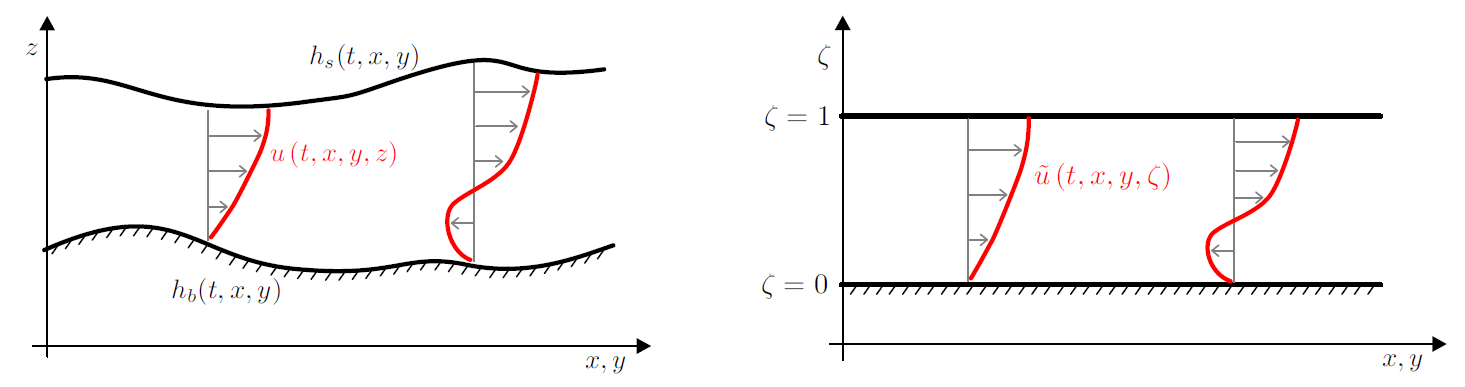
Figure 2: The mapping from physical $z-$space to transformed $\zeta-$space [32].

Using (13), for any function $\Phi(t,x,z)$, the corresponding mapped function in $\zeta-$coordinates is given by

$$\tilde{\Phi}(t,x,\zeta)=\Phi(t,x,z)\zeta+h_{b}(t,x).$$ (14)

The corresponding differential operators read

$$\partial_{\zeta}\tilde{\Phi}=h\partial_{z}\Phi\quad\text{and}\quad h\partial_{s}\Phi=\partial_{s}(h\tilde{\Phi})-\partial_{\zeta}(\partial_{s}(\zeta h+h_{b})\tilde{\Phi}),\quad\text{for}\,\,\,s\in\left[t,x\right].$$ (15)

Taking into account the mapping (13) and using the differential operators (15), the complete vertically resolved system can be written as

$$\partial_{x}\left(h\tilde{u}\right)+\partial_{\zeta}\left[\tilde{w}-\tilde{u}\partial_{x}(\zeta h+h_{b})\right] =0,$$ (16)

$$\begin{split}\partial_{t}(h\tilde{u})+\partial_{x}(h\tilde{u}^{2})+\partial_{\zeta}\left[\tilde{u}\left(\tilde{w}-\tilde{u}\partial_{x}\left(\zeta h+h_{b}\right)-\partial_{t}\left(\zeta h+h_{b}\right)\right)\right]\\ +gh\partial_{x}(h+h_{b})+\frac{gh^{2}}{\rho}(1-\zeta)\partial_{x}\rho&=\frac{1}{\rho}\partial_{\zeta}\tilde{\sigma}_{xz},\end{split}$$ (17)

$$\partial_{t}(h\tilde{c})+\partial_{x}\left(h\tilde{c}\tilde{u}\right)+\partial_{\zeta}\left[\tilde{c}\left(\tilde{w}-\partial_{x}(\zeta h+h_{b})\tilde{u}-\partial_{t}(\zeta h+h_{b})\right)\right] =0.$$ (18)

The system of equations (16) to (18) is referred to as the vertically resolved system in [32] because it incorporates the dependence on the vertical variable $\zeta.$
Furthermore, the boundary conditions (10) and (11) and also the shear stress at the free surface and bottom are mapped to $\zeta-$coordinate as

$$\partial_{t}h_{s}+\left.\tilde{u}\right|_{\zeta=1}\partial_{x}h_{s}-\left.\tilde{w}\right|_{\zeta=1}=0,\quad\quad\quad\quad\quad\quad\quad\left.\tilde{\sigma}_{xz}\right|_{\zeta=1}=0,$$ (19)

$$\partial_{t}h_{b}+\left.\tilde{u}\right|_{\zeta=0}\partial_{x}h_{b}-\left.\tilde{w}\right|_{\zeta=0}=-F_{b},\quad\quad\quad\quad\quad\quad\left.\tilde{\sigma}_{xz}\right|_{\zeta=0}=\,\tau.$$ (20)

Following the second main idea of the Shallow Water Moment model in [32] we expand the horizontal velocity in the vertical variable $\zeta$, using the Legendre polynomial expansion

$$\tilde{u}(t,x,\zeta)=u_{m}(t,x)+\sum_{j=1}^{N}\alpha_{j}(t,x)\phi_{j}(\zeta),$$ (21)

where $u_{m}(t,x)=\displaystyle\int_{0}^{1}\tilde{u}(t,x,\zeta)d\,\zeta$ is the mean of the horizontal velocity, and the basis functions $\phi_{j}(\zeta):[0,1]\rightarrow\mathbb{R}$ are the scaled Legendre polynomials of degree $j\in\mathbb{N}$ defined by

$$\phi_{j}(\zeta)=\frac{1}{j!}\frac{d^{j}}{d\zeta^{j}}(\zeta-\zeta^{2})^{j}.$$ (22)

Therefore, the first scaled and shifted basis functions are

$$\phi_{0}(\zeta)=1,\quad\phi_{1}(\zeta)=1-2\zeta,\quad\phi_{2}(\zeta)=1-6\zeta+6\zeta^{2},\quad\phi_{3}(\zeta)=1-12\zeta+30\zeta^{2}-20\zeta^{3}.$$

These polynomials also satisfy the condition $\phi_{j}(0)=1$, and $\displaystyle\int_{0}^{1}\phi_{j}(\zeta)d\zeta=0.$ In the moment expansion (21), $N\in\mathbb{N}$ denotes both the highest degree of the Legendre polynomial and the order of the velocity expansion. Generally, a larger value of $N$ represents more complex flows. The corresponding basis coefficients $\alpha_{j}(t,x)$ for $j\in\left\{1,\ldots,N\right\}$ are unknown and an additional $N$ equations are derived by projecting momentum balance equation onto Legendre polynomials [32]. These basis coefficients represent the so-called moments and encapsulate the information of horizontal velocity in the vertical $\zeta-$direction.

By employing the moment approach outlined above within our specific framework, we derive the evolution equations for the extended set of variables $(h,hu_{m},h\alpha_{i},hc)^{T}$ for $i\in\{1,\ldots,N\}$. The evolution equations for the water height $h$, the mean horizontal velocity $u_{m}$, and the volumetric sediment concentration $c$ are obtained through the following Galerkin projection of (16), (17), and (18), respectively

$$\langle\cdot,\,1\rangle=\int_{0}^{1}\cdot\,\,d\zeta.$$ (23)

Furthermore, the $N$ evolution equations for the moments are derived by employing a higher-order Galerkin projection of the momentum balance equation (17)

$$\langle\cdot,\,\phi_{i}\rangle=\int_{0}^{1}\cdot\,\phi_{i}(\zeta)\,d\zeta,\quad\quad i=1,\ldots,N.$$ (24)

i.e. multiplying equation (17) by the test function $\phi_{i}(\zeta)$ and subsequently integrating with respect to $\zeta.$

In the three subsequent sections, we provide a detailed derivation of the depth-averaged equations for $h$, $hu_{m}$, and $h\alpha_{i}$. The corresponding derivation for $hc$ is presented within the morphodynamic Section 2.2.1 since morphodynamic change employs suspended sediment concentration.

2.1.2 Depth-averaging the mass balance

To recover an explicit expression for $\tilde{w}$, equation (16) can be written in the following integral form

$$\tilde{w}=-\partial_{x}\left(h\int_{0}^{\zeta}\tilde{u}\,d\hat{\zeta}\right)+\tilde{u}\partial_{x}(\zeta h+h_{b}),$$ (25)

Now, to derive the standard depth-averaged mass balance equation of the shallow water system, we depth-average the transformed mass balance equation, i.e. we apply a projection (23) to an equation (25) and use the kinematic boundary conditions (19) - (20), which yields the following depth-averaged mass balance equation.

$$\partial_{t}h+\partial_{x}(hu_{m})=F_{b}.$$ (26)

Equation (26) represents an equation for the water height $h$, and couples to the equation for the discharge $hu_{m}$, (Section 2.1.3) and the bed exchange rate $F_{b}$ (Section 2.2.3). Without the bed exchange $F_{b}$, equation (26) simplifies to the same as in the SWM [32].

2.1.3 Depth-averaging the momentum equation

The depth-averaged momentum balance equation along the horizontal $x-$axis is derived by applying (23) to (17) and is given by

$$\begin{split}\partial_{t}(hu_{m})+\partial_{x}\left(h\left(u_{m}^{2}+\sum_{j=1}^{N}\frac{\alpha_{j}^{2}}{2j+1}\right)+\frac{gh^{2}}{2}\right)&=-gh\partial_{x}h_{b}+F_{b}u_{b}\\ &-\frac{gh^{2}}{2\rho}(\rho_{s}-\rho_{w})\partial_{x}c-\epsilon|u_{b}|u_{b}.\end{split}$$ (27)

We provide the detailed derivation in Appendix B.1.

Here we only discuss the last three terms on the right-hand side of (27), as they are new compared to the momentum balance equation in [32]:

1. The term $F_{b}u_{b}$ quantifies momentum transfer between flow and erodible bed due to sediment exchange.

2. The term $\displaystyle\frac{gh^{2}}{2\rho}(\rho_{s}-\rho_{w})\partial_{x}c$ represents the effects of spatial variations in sediment concentration.

3. The term $\epsilon|u_{b}|u_{b}$ associates friction within the momentum balance equation. We consider Newtonian Manning friction at the bottom [24] and Newtonian friction within the fluid [24, 32]. Since the Galerkin projection of the momentum balance is influenced only by bottom friction and remains independent of friction within the fluid, we present only the bottom friction in this section, while the treatment of friction within the fluid will be addressed in the subsequent section.
   Accordingly, the Manning friction at the bottom is given by

   $$\left.\tilde{\sigma}_{xz}(\zeta)\right|_{\zeta=0}=-\rho\epsilon|u_{b}|u_{b},$$

   where the bottom velocity is expressed as

   $$u_{b}=\left.\tilde{u}\right|_{\zeta=0}=u_{m}+\displaystyle\sum_{j=1}^{N}\alpha_{j}(t,x)\,\phi_{j}(0)=u_{m}+\sum_{j=1}^{N}\alpha_{j}(t,x),$$ (28)

   and $\epsilon$ is a dimensionless constant defined in [24].

2.1.4 Higher-order moments of the momentum equation

The evolution equations for the higher-order moments of the momentum equation are derived from the higher-order Galerkin projection (24) of (17). Thus, the resulting equation for $h\alpha_{i}$ is given by

$$\begin{split}\partial_{t}(h\alpha_{i})&+\partial_{x}\left(2hu_{m}\alpha_{i}+h\sum_{j,k=1}^{N}\alpha_{j}\alpha_{k}A_{ijk}\right)\\ &=u_{m}\partial_{x}(h\alpha_{i})-\sum_{j,k=1}^{N}B_{ijk}\alpha_{k}\partial_{x}(h\alpha_{j})+F_{b}\left(\alpha_{i}+\sum_{j=1}^{N}\alpha_{j}(H_{ij}-G_{ij})\right)\\ &-\sum_{j=1}^{N}\alpha_{j}G_{ij}\frac{1}{1-\psi}\partial_{x}Q_{b}+(2i+1)\frac{gh^{2}}{\rho}(\rho_{s}-\rho_{w})\frac{\partial c}{\partial x}K_{i}-(2i+1)\left(\epsilon|u_{b}|u_{b}+\frac{\nu}{h}\sum_{j=1}^{N}\alpha_{j}C_{ij}\right),\end{split}$$ (29)

where $A_{ijk},\,B_{ijk},\,G_{ij},\,H_{ij}$ and $K_{i}$ introduced here, are constant coefficients and associated with the integrals of the scaled Legendre polynomials.

$$A_{ijk}=(2i+1)\int_{0}^{1}\phi_{i}\phi_{j}\phi_{k}\,d\zeta,\quad B_{ijk}=(2i+1)\int_{0}^{1}\phi_{i}^{\prime}\left(\phi_{j}d\hat{\zeta}\right)\phi_{k}\,d\zeta,\quad C_{ij}=\int_{0}^{1}\phi_{i}^{\prime}\phi_{j}^{\prime}\,d\zeta,$$ (30)

$$G_{ij}=(2i+1)\int_{0}^{1}\phi_{i}\phi_{j}^{\prime}\,d\zeta,\quad H_{ij}=(2i+1)\int_{0}^{1}\zeta\phi_{i}\phi_{j}^{\prime}\,d\zeta,\quad K_{i}=\int_{0}^{1}\zeta\phi_{i}\,d\zeta$$

We provide the detailed derivation in Appendix B.2.

On the right-hand side of equation (29), four additional terms appear compared to the classical SWM [32]:

1. The term $F_{b}\left(\alpha_{i}+\sum_{j=1}^{N}\alpha_{j}(H_{ij}-G_{ij})\right)$ represents a source term associated with erosion and deposition effects at the bottom, governed by the bed exchange rate $F_{b}.$

2. The term $\sum_{j=1}^{N}\alpha_{j}G_{ij}\frac{1}{1-\psi}\partial_{x}Q_{b},$ which includes the sediment discharge term $Q_{b},$ represents the influence of the bedload transport, as defined in Section 2.2. This term appears in the equations for the higher-order moments since our model does not assume $\partial_{t}h_{b}=0.$

3. The term $(2i+1)\frac{gh^{2}}{\rho}(\rho_{s}-\rho_{w})\frac{\partial c}{\partial x}K_{i}$ arises from the higher order Galerkin projection on the spatial variation of sediment concentration. This term signifies the interaction between suspended sediment and momentum balance.

4. The term $(2i+1)\left(\epsilon|u_{b}|u_{b}+\frac{\nu}{h}\sum_{j=1}^{N}\alpha_{j}C_{ij}\right)$ results from the higher-order Galerkin projection of Manning friction at the bottom i.e., $\left.\tilde{\sigma}_{xz}(\zeta)\right|_{\zeta=0}=-\rho\epsilon|u_{b}|u_{b},$ and Newtonian friction within the fluid i.e., $\left.\tilde{\sigma}_{xz}(\zeta)\right|_{\zeta\in(0,1)}=-\frac{\mu}{h}\partial_{\zeta}\tilde{u}(\zeta)$, and the projection reads

   $$\int_{0}^{1}\phi_{i}\partial_{\zeta}\tilde{\sigma}_{xz}\,d\zeta=\int_{0}^{1}\partial_{\zeta}(\phi_{i}\tilde{\sigma}_{xz})\,d\zeta-\int_{0}^{1}\tilde{\sigma}_{xz}\partial_{\zeta}\phi_{i}\,d\zeta =-\left.\phi_{i}(\zeta)\tilde{\sigma}_{xz}\right|_{\zeta=0}-\frac{\mu}{h}\int_{0}^{1}\phi_{i}^{\prime}\partial_{\zeta}\tilde{u}\,d\zeta$$

   $$=-\rho\epsilon|u_{b}|u_{b}-\frac{\mu}{h}\sum_{j=1}^{N}\int_{0}^{1}\alpha_{j}\phi_{i}^{\prime}\phi_{j}^{\prime}\,d\zeta$$

   $$=-\rho\epsilon|u_{b}|u_{b}-\frac{\mu}{h}\sum_{j=1}^{N}\alpha_{j}C_{ij}$$

2.2 Morphodynamic equations

The morphodynamic part of the model covers the suspended and bedload transport. It consists of the depth-averaged volumetric sediment concentration equation and the Exner equation, respectively, which we explain below.

2.2.1 Depth-averaged volumetric sediment concentration

We derive the depth-averaged volumetric sediment concentration equation by applying the projection (23) to (18), and the resulting equation is given by

$$\partial_{t}(hc)+\partial_{x}(hcu_{m})=(1-\psi)\,F_{b},$$ (31)

where $\psi$ is the porosity of bed material and $F_{b}$ is the bed exchange rate defined in Section 2.2.3 so that $(1-\psi)F_{b}$ describes how much sediment is being exchanged between the bed and the flow.
In this study, we assume a constant sediment concentration profile and do not incorporate a moment expansion for the concentration profile. Including a moment expansion for sediment concentration (or equivalently, density or pressure) would significantly increase the complexity of the model. While this complexity has been explored in models without sediment transport [43], we leave this extension for future work.

2.2.2 Bedload mass balance equation

We use the Exner equation [21, 20] to model the evolution of bedload transport, incorporating the principle of mass conservation for the sediment layer. This formulation represents sediment transport through a flux term, and the right-hand side of the equation includes a source term that describes erosion and deposition processes, which reads as

$$\partial_{t}h_{b}+\frac{1}{1-\psi}\partial_{x}Q_{b}=-F_{b},$$ (32)

where $h_{b}$ is the bed elevation, $Q_{b}$ is the solid sediment discharge, and $F_{b}$ is the bed exchange rate, which accounts for erosion and deposition processes, and defined in Section 2.2.3. More explicitly, the Exner equation represents the rate of bed deformation. Active sediment transport and rapid bed deformation will occur if the flow entrains more sediment particles than it deposits.

The result of the Exner equation (32) is highly dependent on the choice of the sediment discharge formula, $Q_{b}$. We note that there is a plethora of formulas for the sediment discharge term. In this paper, we adopt the following formula [24]

$$Q_{b}=sgn(\tau)\,Q\,\Phi(\theta),$$ (33)

where $Q=\sqrt{\left(\frac{\rho_{s}}{\rho_{w}}-1\right)g\,d_{s}^{3}}$ is the characteristic discharge and $sgn(\cdot)$ is the sign function. We chose the expression (33) for $Q_{b}$ since it depends on the bottom shear stress, used in its non-dimensional form $\theta$ and $Q_{b}$ can be expressed as a function of $\theta$ as $\Phi(\theta).$ The dimensionless bottom shear stress $\theta$ is also called Shields parameter [14] and defined by

$$\theta=\frac{|\tau|}{g\,(\rho_{s}-\rho_{w})\,d_{s}}=\frac{\rho\epsilon|u_{b}|u_{b}}{g\,(\rho_{s}-\rho_{w})\,d_{s}},$$ (34)

where $\epsilon$ is a dimensionless constant [25], $u_{b}$ is the velocity at bottom, as defined in (28), and $d_{s}$ is the diameter of a sediment particle.

There is a framework that includes many different formulas for $\Phi(\theta)$ (see [11, 22, 18, 38, 41]). In this work, we employ the Meyer-Peter $\And$ Müller formula [18]

$$\Phi(\theta)=8(\theta-\theta_{c})_{+}^{3/2},$$ (35)

where $(\cdot)_{+}$ is the positive part and $\theta_{c}$ is the critical shear stress. Notably, sediment transport is initiated only when the Shields parameter $\theta$ exceeds the critical threshold $\theta_{c}$.

2.2.3 Morphological conditions

The bed exchange rate $F_{b}$, used in Section 2.1 and Section 2.2, represents a dynamic equilibrium between two effects: (1) the sediment deposition due to gravitational force and (2) the sediment erosion from the interface due to turbulence. This balance is crucial for understanding sedimentary processes and is defined by

$$F_{b}=\frac{E-D}{1-\psi},$$ (36)

Here $E$ and $D$ denote the erosion and deposition rates, respectively, and $\psi$ is the bedload porosity.
To close the system, we refer [8, 16, 23, 27, 48] and take the following formulas for erosion and deposition.
The sediment erosion and deposition follow from [16, 27], as given by

$$E=\omega_{o}(1-\psi)E_{s},$$ (37)

and

$$D=\omega_{o}c_{b},$$ (38)

where

• $\omega_{o}$ is the settling velocity determined by [48],

  $$\omega_{o}=\sqrt{\left(\frac{13.95\nu_{w}}{d_{s}}\right)^{2}+1.09\,\rho_{w}\left(\frac{\rho_{s}}{\rho_{w}}-1\right)gd_{s}}-\frac{13.95\nu_{w}}{d_{s}},$$ (39)

• $\nu_{w}$ is the kinematic viscosity of water and $d_{s}$ is the diameter of sediment particle

• $E_{s}$ is the sediment erosion coefficient and computed by [23],

  $$E_{s}=\frac{1.3\times 10^{-7}\mathcal{Z}^{5}}{1+4.3\times 10^{-7}\mathcal{Z}^{5}},$$ (40)

• $\mathcal{Z}=\displaystyle\frac{\gamma_{1}\sqrt{c_{D}}|u_{b}|}{\omega_{o}}\mathcal{R}^{\gamma_{2}}_{p}$ with particle Reynolds number $\mathcal{R}_{p}=\displaystyle\frac{\sqrt{(\rho_{s}-\rho_{w})gd_{s}}d_{s}}{\nu_{w}}$, $u_{b}$ the bottom velocity, and $c_{D}$ the bed drag coefficient

• $\gamma_{1},\gamma_{2}$ are two parameters depending on $\mathcal{R}_{p}$ [27]

  $$\left(\gamma_{1},\gamma_{2}\right)=\begin{cases}\left(1,0.6\right),&\text{if $\mathcal{R}_{p}>2.36$}\\ \left(0.586,1.23\right),&\text{if $\mathcal{R}_{p}\leq 2.36$}\end{cases}$$

• $c_{b}$ is the fractional concentration of sediment suspension near the bed and defined by [8]

  $$c_{b}=c(t,x)\,\left(0.4\left(\frac{d_{s}}{D_{sg}}\right)^{1.64}+1.64\right),$$ (41)

  with $c(t,x)$ the volumetric sediment concentration and $D_{sg}$ the geometric mean size of the suspended sediment mixture. In the work, we assume all the particles are of equal size, i.e., $D_{sg}=d_{s}$.

2.3 Coupled hydro-morphodynamic model

By incorporating the derivations and definitions outlined in Section 2.1 and Section 2.2, we obtain a closed Shallow Water Exner Moment model with Erosion and Deposition (SWEMED), consisting of a total of $N+4$ coupled equations (42) for the set of convective variables $(h,hu_{m},h\alpha_{1},\ldots,h\alpha_{N},hc,h_{b})^{T}\in\mathbb{R}^{N+4}$, where $N$ denotes the highest degree of the Legendre polynomial expansions which is also called the order of the moment model.

$$\underbrace{1}_{\text{mass balance}}+\underbrace{1}_{\text{momentum equation}}+\underbrace{N}_{\text{moment equations}}+{\color[rgb]{0,0,0}\underbrace{1}_{\text{sediment concentration}}}+{\color[rgb]{0,0,0}\underbrace{1}_{\text{bedload mass balance}}}=\,N+4$$

Thus the coupled model is formulated as follows

$$\left\{\begin{aligned} &\partial_{t}h+\partial_{x}(hu_{m})&&=\frac{E-D}{1-\psi},\\ &\partial_{t}(hu_{m})+\partial_{x}\left(h\left(u_{m}^{2}+\sum_{j=1}^{N}\frac{\alpha_{j}^{2}}{2j+1}\right)+\frac{gh^{2}}{2}\right)&&=-gh\partial_{x}h_{b}-\frac{gh^{2}}{2\rho}(\rho_{s}-\rho_{w})\partial_{x}c\\ &&&\quad+\frac{(E-D)u_{b}}{1-\psi}-\epsilon|u_{b}|u_{b},\\ &\partial_{t}(h\alpha_{i})+\partial_{x}\left(2hu_{m}\alpha_{i}+h\sum_{j,k=1}^{N}\alpha_{j}\alpha_{k}A_{ijk}\right)&&=u_{m}\partial_{x}(h\alpha_{i})-\sum_{j,k=1}^{N}B_{ijk}\alpha_{k}\partial_{x}(h\alpha_{j})\\ &&&\quad+(2i+1)\frac{gh^{2}}{\rho}(\rho_{s}-\rho_{w})\frac{\partial c}{\partial x}K_{i}\\ &&&\quad+\frac{E-D}{1-\psi}\left(\alpha_{i}+\sum_{j=1}^{N}\alpha_{j}(H_{ij}-G_{ij})\right)\\ &&&\quad-(2i+1)\left(\epsilon|u_{b}|u_{b}+\frac{\nu}{h}\sum_{j=1}^{N}\alpha_{j}C_{ij}\right)\\ &&&\quad-\sum_{j=1}^{N}\alpha_{j}G_{ij}\displaystyle\partial_{x}\left(\frac{Q_{b}}{1-\psi}\right),\\ &\partial_{t}(hc)+\partial_{x}(hcu_{m})&&=E-D,\\ &\partial_{t}h_{b}+\displaystyle\partial_{x}\left(\frac{Q_{b}}{1-\psi}\right)&&=\frac{D-E}{1-\psi}.\end{aligned}\right.$$ (42)

We can write the complete system (42) as a first-order PDE with conservative, non-conservative, and source terms, which reads

$$\partial_{t}W+\frac{\partial F}{\partial W}\partial_{x}{\color[rgb]{0,0,0}W}\,=B\partial_{x}W-A_{s}\partial_{x}W+S_{F}+S_{ED}.$$ (43)

In the left-hand side of (43), the jacobian of the conservative flux is given by

$$\medmath{\frac{\partial F}{\partial W}=\begin{pmatrix}0&1&0&\dots&0&0&0\\ gh-u_{m}^{2}-\displaystyle\sum_{j=1}^{N}\frac{\alpha_{j}^{2}}{2j+1}&2u_{m}&\frac{2\alpha_{1}}{2\cdot 1+1}&\dots&\frac{2\alpha_{N}}{2\cdot N+1}&0&0\\ -2u_{m}\alpha_{1}-\displaystyle\sum_{j,k=1}^{N}A_{1jk}\alpha_{j}\alpha_{k}&2\alpha_{1}&2u_{m}+2\displaystyle\sum_{k=1}^{N}A_{11k}\alpha_{k}&\dots&2\displaystyle\sum_{k=1}^{N}A_{1Nk}\alpha_{k}&0&0\\ \vdots&\vdots&\hskip 85.35826pt\ddots&&&\vdots&\vdots\\ \vdots&\vdots&&\hskip-2.84526pt\ddots&&\vdots&\vdots\\ -2u_{m}\alpha_{N}-\displaystyle\sum_{j,k=1}^{N}A_{Njk}\alpha_{j}\alpha_{k}&2\alpha_{N}&2\displaystyle\sum_{k=1}^{N}A_{N1k}\alpha_{k}&\dots&2u_{m}+2\displaystyle\sum_{k=1}^{N}A_{NNk}\alpha_{k}&0&0\\ -cu_{m}&-c&0&\ldots&0&u_{m}&0\\ \delta_{h}&\delta_{q}&\delta_{q}&\dots&\delta_{q}&\delta_{c}&0\end{pmatrix},}$$

where

$$\delta_{q}=\frac{\partial}{\partial_{hu_{m}}}\left(\frac{Q_{b}}{1-\psi}\right)=\frac{24Q}{1-\psi}sgn(\tau)\frac{\rho\epsilon}{g(\rho_{s}-\rho_{w})d_{s}}\left(\theta-\theta_{c}\right)_{+}^{1/2}\frac{u_{b}}{h},$$ (44a)

$$\delta_{h}=\frac{\partial}{\partial_{h}}\left(\frac{Q_{b}}{1-\psi}\right)=-u_{b}\left(1+\displaystyle\frac{c(t,x)\left(\rho_{s}-\rho_{w}\right)}{2\rho}\right)\delta_{q},$$ (44b)

$$\delta_{c}=\frac{\partial}{\partial_{hc}}\left(\frac{Q_{b}}{1-\psi}\right)=u_{b}\displaystyle\left(\frac{\rho_{s}-\rho_{w}}{2\rho}\right)\delta_{q},$$ (44c)

and

$$\frac{\partial}{\partial_{h\alpha_{i}}}\left(\frac{Q_{b}}{1-\psi}\right)=\delta_{q}\quad\quad i\in\left\{1,\ldots,N\right\},$$ (44d)

with bottom velocity $u_{b}$ and the Shields parameter $\theta$ defined in (28) and (34), respectively.
On the right-hand side of (43), the non-conservative matrix reads

$$\medmath{B=\begin{pmatrix}0&0&0&\dots&0&0&0\\ \displaystyle\frac{gh(\rho-\rho_{w})}{2\rho}&0&0&\dots&0&\displaystyle\frac{-gh(\rho_{s}-\rho_{w})}{2\rho}&-gh\\ \displaystyle\frac{gh(\rho-\rho_{w})}{2\rho}&0&u_{m}-\displaystyle\sum_{k=1}^{N}B_{11k}\alpha_{k}&\dots&-\displaystyle\sum_{k=1}^{N}B_{1Nk}\alpha_{k}&\displaystyle\frac{-gh(\rho_{s}-\rho_{w})}{2\rho}&0\\ \vdots&\vdots&\hskip 85.35826pt\ddots&&&\vdots&\vdots\\ \vdots&\vdots&&\hskip-2.84526pt\ddots&&\vdots&\vdots\\ 0&0&-\displaystyle\sum_{k=1}^{N}B_{N1k}\alpha_{k}&\dots&u_{m}-\displaystyle\sum_{k=1}^{N}B_{NNk}\alpha_{k}&0&0\\ 0&0&0&\dots&0&0&0\\ 0&0&0&\dots&0&0&0\\ \end{pmatrix},}$$

and the sediment discharge matrix $A_{s}$ is resulting from $\displaystyle\sum_{j=1}^{N}\alpha_{j}G_{ij}\partial_{x}\left(\frac{Q_{b}}{1-\psi}\right)$ and reads

$$\medmath{A_{s}=\begin{pmatrix}0&0&0&\dots&0&0&0\\ 0&0&0&\dots&0&0&0\\ \displaystyle\sum_{j=1}^{N}\alpha_{j}G_{1j}\delta_{h}&\displaystyle\sum_{j=1}^{N}\alpha_{j}G_{1j}\delta_{q}&\displaystyle\sum_{j=1}^{N}\alpha_{j}G_{1j}\delta_{q}&\dots&\displaystyle\sum_{j=1}^{N}\alpha_{j}G_{1j}\delta_{q}&\displaystyle\sum_{j=1}^{N}\alpha_{j}G_{1j\delta_{c}}&0\\ \displaystyle\sum_{j=1}^{N}\alpha_{j}G_{2j}\delta_{h}&\displaystyle\sum_{j=1}^{N}\alpha_{j}G_{2j}\delta_{q}&\displaystyle\sum_{j=1}^{N}\alpha_{j}G_{2j}\delta_{q}&\dots&\displaystyle\sum_{j=1}^{N}\alpha_{j}G_{2j}\delta_{q}&\displaystyle\sum_{j=1}^{N}\alpha_{j}G_{2j\delta_{c}}&0\\ \vdots&\vdots&\hskip 85.35826pt\ddots&&&\vdots&\vdots\\ \vdots&\vdots&&\hskip-2.84526pt\ddots&&\vdots&\vdots\\ \displaystyle\sum_{j=1}^{N}\alpha_{j}G_{Nj}\delta_{h}&\displaystyle\sum_{j=1}^{N}\alpha_{j}G_{Nj}\delta_{q}&\displaystyle\sum_{j=1}^{N}\alpha_{j}G_{Nj}\delta_{q}&\dots&\displaystyle\sum_{j=1}^{N}\alpha_{j}G_{Nj}\delta_{q}&\displaystyle\sum_{j=1}^{N}\alpha_{j}G_{Nj\delta_{c}}&0\\ 0&0&0&\dots&0&0&0\\ 0&0&0&\dots&0&0&0\\ \end{pmatrix}.}$$

The source terms $S_{F,i}$ and $S_{ED,i}$ result from the combined effects of friction and the processes of erosion and deposition, respectively, and are given by

$$S_{F,i}=\begin{cases}0,&\quad\text{if $i=1,N+3,N+4,$}\\ -\epsilon|u_{b}|u_{b},&\quad\text{if $i=2,$}\\ -(2i+1)\displaystyle\left(\epsilon|u_{b}|u_{b}+\displaystyle\frac{\nu}{h}\displaystyle\sum_{j=1}^{N}\alpha_{j}C_{ij}\right),&\quad\text{if $i\in\left\{3,\ldots,N+2\right\},$}\end{cases}$$

and

$$S_{ED,i}=\begin{cases}\displaystyle\frac{E-D}{1-\psi},&\text{if $i=1,$}\\ \displaystyle\frac{(E-D)u_{b}}{1-\psi},&\text{if $i=2,$}\\ \displaystyle\frac{E-D}{1-\psi}\left(\alpha_{i}+\displaystyle\sum_{j=1}^{N}\alpha_{j}(H_{ij}-G_{ij})\right),&\text{if $i\in\left\{3,\ldots,N+2\right\},$}\\ E-D,&\text{if $i=N+3,$}\\ \displaystyle\frac{D-E}{1-\psi},&\text{if $i=N+4.$}\\ \end{cases}$$

The resulting system (43) can be written in the form

$$\partial_{t}\,W+A_{ED}(W)\partial_{x}\,W=S(W),$$ (45)

where we define the state vector of conservative variables as ${\color[rgb]{0,0,0}W}=(h,hu_{m},h\alpha_{1},.....,h\alpha_{N},hc,h_{b})^{T}\in\mathbb{R}^{N+4}$. We express the transport matrix in explicit form as $A_{ED}(W)=\left(\displaystyle\frac{\partial F}{\partial W}-B+A_{s}\right)\in\mathbb{R}^{(N+4)\times(N+4)}$. Additionally, the right-hand side of (45) $S(W)=(S_{F}+S_{ED})\in\mathbb{R}^{N+4}$ models the source term, which arises from friction and the considerations of erosion and deposition.

2.3.1 Lower-order moments of SWEMED

In this section, we present the structural framework of lower-order moments of the SWEMED namely, the zeroth-order $(N=0)$, first-order $(N=1)$, second-order $(N=2)$ and third-order $(N=3)$ formulations as representative examples. We introduce these particular formulations here because they serves as the foundation for the numerical simulations presented later in the Section 4.

2.3.1.1   SWEMED0

Considering $N=0$ the zeroth-order moment represents a uniform velocity profile in the vertical direction, i.e., $u(t,x,\zeta)=u_{m}(t,x)$. The zeroth-order Shallow Water Exner Moment model with Erosion and Deposition (SWEMED0) is identical to the standard Shallow Water Exner model with Erosion and Deposition (SWEED) and reads

$$\partial_{t}\begin{pmatrix}\displaystyle h\\ \displaystyle hu_{m}\\ \displaystyle hc\\ \displaystyle h_{b}\end{pmatrix}+\partial_{x}F=B\,\partial_{x}\begin{pmatrix}h\\ hu_{m}\\ hc\\ h_{b}\end{pmatrix}-A_{s}\partial_{x}\begin{pmatrix}h\\ hu_{m}\\ hc\\ h_{b}\end{pmatrix}+S_{F}+S_{ED},$$ (46)

$$\text{ with}\quad F=\begin{pmatrix}h\\ \displaystyle hu_{m}^{2}+\frac{1}{2}gh^{2}\\ hcu_{m}\\ \displaystyle\frac{Q_{b}}{1-\psi}\end{pmatrix},\quad\frac{\partial F}{\partial W}=\begin{pmatrix}0&1&0&0\\ gh-u^{2}_{m}&2u_{m}&0&0\\ -cu_{m}&c&u_{m}&0\\ \delta_{h}&\delta_{q}&\delta_{c}&0\end{pmatrix},$$

$$B=\begin{pmatrix}0&0&0&0\\ \displaystyle\frac{gh(\rho-\rho_{w})}{2\rho}&0&\displaystyle\frac{-gh(\rho_{s}-\rho_{w})}{2\rho}&-gh\\ 0&0&0&0\\ 0&0&0&0\end{pmatrix},\quad S_{F}=\begin{pmatrix}0\\ -\epsilon|u_{m}|u_{m}\\ 0\\ 0\end{pmatrix},\quad\text{and}\quad S_{ED}=\displaystyle\frac{E-D}{1-\psi}\begin{pmatrix}1\\ u_{m}\\ 1-\psi\\ -1\end{pmatrix},$$

leading to the transport matrix

$$A_{ED}=\frac{\partial F}{\partial W}-B+A_{s}=\begin{pmatrix}0&1&0&0\\ gh-u^{2}_{m}-\displaystyle\frac{gh(\rho-\rho_{w})}{2\rho}&2u_{m}&\displaystyle\frac{gh(\rho_{s}-\rho_{w})}{2\rho}&gh\\ -cu_{m}&c&u_{m}&0\\ \delta_{h}&\delta_{q}&\delta_{c}&0\end{pmatrix}$$ (47)

where the sediment discharge matrix, $A_{s}=\mathbf{0}\in\mathbb{R}^{4\times 4}$. We see from (80) that $A_{s}$ is resulting from $\displaystyle\sum_{j=1}^{N}\alpha_{j}G_{ij}\partial_{x}\left(\frac{Q_{b}}{1-\psi}\right)$, representing the projection associated with the vertical coupling term and only appears in higher-order averaged models, where such coupling effects are included, since our model does not assume $\partial_{t}h_{b}=0$.

2.3.1.2   SWEMED1

With $N=1$ the first-order moment represents the linear change of velocity in vertical direction, i.e. $u(t,x,\zeta)=u_{m}(t,x)+\alpha_{1}(t,x,\zeta)\phi_{1}(\zeta)$, where $\phi_{1}(\zeta)$ is the linear Legendre basis function defined in (22). Thus the first-order Shallow Water Exner Moment model with Erosion and Deposition (SWEMED1) reads

$$\partial_{t}\begin{pmatrix}h\\ hu_{m}\\ h\alpha_{1}\\ hc\\ h_{b}\end{pmatrix}+\partial_{x}F=B\partial_{x}\begin{pmatrix}h\\ hu_{m}\\ h\alpha_{1}\\ hc\\ h_{b}\end{pmatrix}-A_{s}\partial_{x}\begin{pmatrix}h\\ hu_{m}\\ h\alpha_{1}\\ hc\\ h_{b}\end{pmatrix}+S_{F}+S_{ED},$$ (48)

with

$$F=\begin{pmatrix}hu_{m}\\ hu_{m}^{2}+\frac{1}{2}gh^{2}+\frac{1}{3}h\alpha^{2}_{1}\\ 2hu_{m}\alpha_{1}\\ hcu_{m}\\ \frac{Q_{b}}{1-\psi}\end{pmatrix},\quad\frac{\partial F}{\partial W}=\begin{pmatrix}0&1&0&0&0\\ gh-u^{2}_{m}-\frac{\alpha^{2}_{1}}{3}&2u_{m}&\frac{2\alpha_{1}}{3}&0&0\\ -2\alpha_{1}u_{m}&2\alpha_{1}&2u_{m}&0&0\\ -cu_{m}&c&0&u_{m}&0\\ \delta_{h}&\delta_{q}&\delta_{q}&\delta_{c}&0\end{pmatrix},$$

$$B=\begin{pmatrix}0&0&0&0&0\\ \displaystyle\frac{gh(\rho-\rho_{w})}{2\rho}&0&0&-\displaystyle\frac{gh(\rho_{s}-\rho_{w})}{2\rho}&-gh\\ \displaystyle\frac{gh(\rho-\rho_{w})}{2\rho}&0&u_{m}&-\displaystyle\frac{gh(\rho_{s}-\rho_{w})}{2\rho}&0\\ 0&0&0&0&0\\ 0&0&0&0&0\\ \end{pmatrix},$$

$$S_{F}=\begin{pmatrix}0\\ -\epsilon|u_{m}+\alpha_{1}|(u_{m}+\alpha_{1})\\ -3\epsilon|u_{m}+\alpha_{1}|(u_{m}+\alpha_{1})-12\displaystyle\frac{\nu}{h}\alpha_{1}\\ 0\\ 0\end{pmatrix},\quad S_{ED}=\displaystyle\frac{E-D}{1-\psi}\begin{pmatrix}1\\ u_{m}+\alpha_{1}\\ 2\alpha_{1}\\ 1-\psi\\ -1\end{pmatrix},$$

leading to the transport matrix

$$A_{ED}=\displaystyle\frac{\partial F}{\partial W}-B+A_{s}=\begin{pmatrix}0&1&0&0&0\\ gh-u^{2}_{m}-\displaystyle\frac{\alpha^{2}_{1}}{3}-\displaystyle\frac{gh(\rho-\rho_{w})}{2\rho}&2u_{m}&\displaystyle\frac{2\alpha_{1}}{3}&\displaystyle\frac{gh(\rho_{s}-\rho_{w})}{2\rho}&gh\\ -2\alpha_{1}u_{m}-\displaystyle\frac{gh(\rho-\rho_{w})}{2\rho}&2\alpha_{1}&u_{m}&\displaystyle\frac{gh(\rho_{s}-\rho_{w})}{2\rho}&0\\ -cu_{m}&c&0&u_{m}&0\\ \delta_{h}&\delta_{q}&\delta_{q}&\delta_{c}&0\end{pmatrix},$$ (49)

where the sediment discharge matrix, $A_{s}=\mathbf{0}\in\mathbb{R}^{5\times 5}$ as $A_{s}=\displaystyle\sum_{j=1}^{N}\alpha_{j}G_{ij}\partial_{x}\left(\frac{Q_{b}}{1-\psi}\right)$ involves $G_{ij}$ defined in (30) and clearly $G_{11}=\displaystyle\int_{0}^{1}\phi_{1}(\zeta)\,\phi_{1}^{\prime}(\zeta)\,d\zeta=0.$

2.3.1.3   SWEMED2

The second-order moment $N=2$ corresponds to a quadratic velocity profile in the vertical direction, which is expressed as $u(t,x,\zeta)=u_{m}(t,x)+\alpha_{1}(t,x)\phi_{1}(\zeta)+\alpha_{2}(t,x)\phi_{2}(\zeta)$, resulting in the second-order Shallow Water Exner Moment Model with Erosion and Deposition (SWEMED2). In this formulation, $\phi_{1}(\zeta)$ and $\phi_{2}(\zeta)$ are the linear and quadratic Legendre basis functions, respectively, defined in (22). Thus the SWEMED2 reads

$$\partial_{t}\begin{pmatrix}h\\ hu_{m}\\ h\alpha_{1}\\ h\alpha_{2}\\ hc\\ h_{b}\end{pmatrix}+\partial_{x}F=B\partial_{x}\begin{pmatrix}h\\ hu_{m}\\ h\alpha_{1}\\ h\alpha_{2}\\ hc\\ h_{b}\end{pmatrix}-A_{s}\partial_{x}\begin{pmatrix}h\\ hu_{m}\\ h\alpha_{1}\\ h\alpha_{2}\\ hc\\ h_{b}\end{pmatrix}+S_{F}+S_{ED},$$ (50)

with

$$F=\begin{pmatrix}hu_{m}\\ hu_{m}^{2}+\frac{1}{2}gh^{2}+\frac{1}{3}h\alpha^{2}_{1}+\frac{1}{5}h\alpha^{2}_{2}\\ 2hu_{m}\alpha_{1}+\frac{4}{5}h\alpha_{1}\alpha_{2}\\ 2hu_{m}\alpha_{2}+\frac{2}{3}h\alpha^{2}_{1}+\frac{2}{7}h\alpha^{2}_{2}\\ hcu_{m}\\ \frac{Q_{b}}{1-\psi}\end{pmatrix},\quad\frac{\partial F}{\partial W}=\begin{pmatrix}0&1&0&0&0&0\\ gh-u^{2}_{m}-\frac{\alpha^{2}_{1}}{3}-\frac{\alpha^{2}_{2}}{5}&2u_{m}&\frac{2\alpha_{1}}{3}&\frac{2\alpha_{2}}{5}&0&0\\ -2\alpha_{1}u_{m}-\frac{4}{5}\alpha_{1}\alpha_{2}&2\alpha_{1}&2u_{m}+\frac{4\alpha_{2}}{5}&\frac{4\alpha_{1}}{5}&0&0\\ -\frac{2}{3}\alpha^{2}_{1}-2u_{m}\alpha_{2}-\frac{2}{7}\alpha^{2}_{2}&2\alpha_{2}&\frac{4\alpha_{1}}{3}&2u_{m}+\frac{4\alpha_{2}}{7}&0&0\\ -cu_{m}&c&0&0&u_{m}&0\\ \delta_{h}&\delta_{q}&\delta_{q}&\delta_{q}&\delta_{c}&0\end{pmatrix},$$

$$B=\begin{pmatrix}0&0&0&0&0&0\\ \displaystyle\frac{gh(\rho-\rho_{w})}{2\rho}&0&0&0&-\displaystyle\frac{gh(\rho_{s}-\rho_{w})}{2\rho}&-gh\\ \displaystyle\frac{gh(\rho-\rho_{w})}{2\rho}&0&u_{m}-\displaystyle\frac{\alpha_{2}}{5}&\displaystyle\frac{\alpha_{1}}{5}&-\displaystyle\frac{gh(\rho_{s}-\rho_{w})}{2\rho}&0\\ 0&0&\alpha_{1}&u_{m}+\displaystyle\frac{\alpha_{2}}{7}&0&0\\ 0&0&0&0&0&0\\ 0&0&0&0&0&0\\ \end{pmatrix},$$

$$A_{s}=\begin{pmatrix}\mathbf{0}_{1\times 6}\\ \mathbf{r}\\ \mathbf{0}_{4\times 6}\end{pmatrix},\quad\text{where}\quad\mathbf{r}=-6\alpha_{2}\left(\delta_{h},\ \delta_{q},\ \delta_{q},\ \delta_{q},\ \delta_{c},\ 0\right),$$

$$S_{F}=\begin{pmatrix}0\\ -\epsilon|u_{m}+\alpha_{1}+\alpha_{2}|(u_{m}+\alpha_{1}+\alpha_{2})\\ -3\epsilon|u_{m}+\alpha_{1}+\alpha_{2}|(u_{m}+\alpha_{1}+\alpha_{2})-12\displaystyle\frac{\nu}{h}\alpha_{1}\\ -5\epsilon|u_{m}+\alpha_{1}+\alpha_{2}|(u_{m}+\alpha_{1}+\alpha_{2})\,-60\,\,\displaystyle\frac{\nu}{h}\alpha_{2}\\ 0\\ 0\end{pmatrix},\quad S_{ED}=\displaystyle\frac{E-D}{1-\psi}\begin{pmatrix}1\\ u_{m}+\alpha_{1}+\alpha_{2}\\ 2\alpha_{1}+3\alpha_{2}\\ 3\alpha_{2}\\ 1-\psi\\ -1\end{pmatrix},$$

leading to the transport matrix

$$A_{ED}=\displaystyle\frac{\partial F}{\partial W}-B+A_{s}=\begin{pmatrix}0&1&0&0&0&0\\ gh-u^{2}_{m}-\frac{\alpha^{2}_{1}}{3}-\frac{\alpha^{2}_{2}}{5}-\frac{gh(\rho-\rho_{w})}{2\rho}&2u_{m}&\frac{2\alpha_{1}}{3}&\frac{2\alpha_{2}}{5}&\frac{gh(\rho_{s}-\rho_{w})}{2\rho}&gh\\ -2\alpha_{1}u_{m}-\frac{4}{5}\alpha_{1}\alpha_{2}-\frac{gh(\rho-\rho_{w})}{2\rho}&2\alpha_{1}&u_{m}+\alpha_{2}&\frac{3\alpha_{1}}{5}&\frac{gh(\rho_{s}-\rho_{w})}{2\rho}&0\\ -\frac{2}{3}\alpha^{2}_{1}-2u_{m}\alpha_{2}-\frac{2}{7}\alpha^{2}_{2}&2\alpha_{2}&\frac{\alpha_{1}}{3}&u_{m}+\frac{3\alpha_{2}}{7}&0&0\\ -cu_{m}&c&0&0&u_{m}&0\\ \delta_{h}&\delta_{q}&\delta_{q}&\delta_{q}&\delta_{c}&0\end{pmatrix}.$$ (51)

2.3.1.4   SWEMED3

The third-order moment $N=3$ corresponds to a cubic velocity profile in the vertical direction, which is expressed as $u(t,x,\zeta)=u_{m}(t,x)+\alpha_{1}(t,x)\phi_{1}(\zeta)+\alpha_{2}(t,x)\phi_{2}(\zeta)+\alpha_{3}(t,x)\phi_{3}(\zeta)$, resulting in the third-order Shallow Water Exner Moment model with Erosion and Deposition (SWEMED3). In this formulation, $\phi_{1}(\zeta)$, $\phi_{2}(\zeta)$ and $\phi_{3}(\zeta)$ are the linear, quadratic, and cubic Legendre basis functions, respectively, defined in (22). Thus the SWEMED3 reads

$$\partial_{t}\begin{pmatrix}h\\ hu_{m}\\ h\alpha_{1}\\ h\alpha_{2}\\ h\alpha_{3}\\ hc\\ h_{b}\end{pmatrix}+\partial_{x}\begin{pmatrix}hu_{m}\\ hu_{m}^{2}+\frac{1}{2}gh^{2}+\frac{1}{3}h\alpha^{2}_{1}+\frac{1}{5}h\alpha^{2}_{2}+\frac{1}{7}h\alpha^{2}_{3}\\ 2hu_{m}\alpha_{1}+\frac{4}{5}h\alpha_{1}\alpha_{2}+\frac{18}{35}h\alpha_{2}\alpha_{3}\\ 2hu_{m}\alpha_{2}+\frac{2}{3}h\alpha^{2}_{1}+\frac{2}{7}h\alpha^{2}_{2}+\frac{4}{21}h\alpha^{2}_{3}+\frac{6}{7}h\alpha_{1}\alpha_{3}\\ 2hu_{m}\alpha_{3}+\frac{6}{5}h\alpha_{1}\alpha_{2}+\frac{8}{15}h\alpha_{2}\alpha_{3}\\ hcu_{m}\\ \frac{Q_{b}}{1-\psi}\end{pmatrix}=B\partial_{x}\begin{pmatrix}h\\ hu_{m}\\ h\alpha_{1}\\ h\alpha_{2}\\ h\alpha_{3}\\ hc\\ h_{b}\end{pmatrix}-A_{s}\partial_{x}\begin{pmatrix}h\\ hu_{m}\\ h\alpha_{1}\\ h\alpha_{2}\\ h\alpha_{3}\\ hc\\ h_{b}\end{pmatrix}+S\begin{pmatrix}h\\ hu_{m}\\ h\alpha_{1}\\ h\alpha_{2}\\ h\alpha_{3}\\ hc\\ h_{b}\end{pmatrix}.$$ (52)

The transport matrix

$$A_{ED}=\begin{pmatrix}0&1&0&0&0&0&0\\ gh-u^{2}_{m}-\frac{\alpha^{2}_{1}}{3}-\frac{\alpha^{2}_{2}}{5}-\frac{\alpha^{2}_{3}}{7}-\frac{gh(\rho-\rho_{w})}{2\rho}&2u_{m}&\frac{2\alpha_{1}}{3}&\frac{2\alpha_{2}}{5}&\frac{2\alpha_{3}}{7}&\frac{gh(\rho_{s}-\rho_{w})}{2\rho}&gh\\ -\frac{2}{37}(9\alpha_{3}\alpha_{2}+7\alpha_{1}(5u_{m}+2\alpha_{2}))-\frac{gh(\rho-\rho_{w})}{2\rho}&2\alpha_{1}&u_{m}+\alpha_{2}&\frac{3(\alpha_{1}+\alpha_{3})}{5}&\frac{3\alpha_{2}}{7}&\frac{gh(\rho_{s}-\rho_{w})}{2\rho}&0\\ -\frac{2}{21}(7\alpha^{2}_{1}+9\alpha_{1}\alpha_{3}+2\alpha^{2}_{3}+3\alpha_{2}(7u_{m}+\alpha_{2}))&2\alpha_{2}&\frac{\alpha_{1}}{3}+\frac{9\alpha_{3}}{7}&u_{m}+\frac{3\alpha_{2}}{7}&\frac{4\alpha_{1}}{7}+\frac{\alpha_{3}}{3}&0&0\\ -\frac{2}{15}(15u_{m}\alpha_{3}+4\alpha_{2}\alpha_{3}+9\alpha_{1}\alpha_{2})&2\alpha_{3}&0&\frac{2(\alpha_{1}+\alpha_{3})}{5}&u_{m}+\frac{\alpha_{2}}{3}&0&0\\ -cu_{m}&c&0&0&0&u_{m}&0\\ \delta_{h}&\delta_{q}&\delta_{q}&\delta_{q}&\delta_{q}&\delta_{c}&0\end{pmatrix},$$ (53)

with

$$S_{F}=\begin{pmatrix}0\\ -\epsilon|u_{m}+\alpha_{1}+\alpha_{2}+\alpha_{3}|(u_{m}+\alpha_{1}+\alpha_{2}+\alpha_{3})\\ -3\epsilon|u_{m}+\alpha_{1}+\alpha_{2}+\alpha_{3}|(u_{m}+\alpha_{1}+\alpha_{2}+\alpha_{3})-12\displaystyle\frac{\nu}{h}(\alpha_{1}+\alpha_{3})\\ -5\epsilon|u_{m}+\alpha_{1}+\alpha_{2}+\alpha_{3}|(u_{m}+\alpha_{1}+\alpha_{2}+\alpha_{3})\,-60\,\,\displaystyle\frac{\nu}{h}\alpha_{2}\\ -7\epsilon|u_{m}+\alpha_{1}+\alpha_{2}+\alpha_{3}|(u_{m}+\alpha_{1}+\alpha_{2}+\alpha_{3})-7\displaystyle\frac{\nu}{h}(4\alpha_{1}+24\alpha_{3})\\ 0\\ 0\end{pmatrix},\quad S_{ED}=\displaystyle\frac{E-D}{1-\psi}\begin{pmatrix}1\\ u_{m}+\alpha_{1}+\alpha_{2}+\alpha_{3}\\ 2\alpha_{1}+3(\alpha_{2}+\alpha_{3})\\ 3\alpha_{2}+5\alpha_{3}\\ 4\alpha_{3}\\ 1-\psi\\ -1\end{pmatrix}.$$

In the next section, we will discuss the hyperbolicity of the SWEMED for bedload and suspended load sediment transport.

3 Hyperbolic SWEMED for sediment transport

Hyperbolicity ensures a finite propagation speed of the waves, which is fundamental for dealing with flow problems. Additionally, it supports the well-posedness of initial value problem, numerical stability, and convergence of solutions [10, 30].
To define the hyperbolicity of a first-order partial differential equation of the form

$$\partial_{t}U+A(U)\partial_{x}U=0.$$ (54)

we use the following definition [19, 31]

Definition 3.1.

The system (54) is hyperbolic if $A(U)$ is diagonalizable with real eigenvalues for all states of $U.$ If $A(U)$ has distinct real eigenvalues, then it is called strictly hyperbolic.

To illustrate, consider the SWEMED0 system from (46). The system of equations (46) is classified as hyperbolic if the characteristic polynomial associated with the transport matrix $A_{ED}\in\mathbb{R}^{4\times 4}$ (47) is found to have four distinct real roots. The characteristic polynomial is given by

$$\chi_{A_{ED}}(\lambda)=(u_{m}-\lambda)\left[(-\lambda)\left((\lambda-u_{m})^{2}-gh\right)+gh(\delta_{h}+\lambda\delta_{q}+c\delta_{c})\right]=(u_{m}-\lambda)\left[f(\lambda)+d(\lambda)\right],$$ (55)

where $f(\lambda)=(-\lambda)\left((\lambda-u_{m})^{2}-gh\right)$ and $d(\lambda)=gh(\delta_{h}+\lambda\delta_{q}+c\delta_{c})$.

A detailed analysis of hyperbolicity in shallow water models incorporating both bedload and suspended load sediment transport, as presented in [14, 27], demonstrates that when the Meyer-Peter & Müller formula is employed to describe sediment discharge, $Q_{b}$ (see equation (33)), the system (46) satisfies the necessary conditions for hyperbolicity.

Similarly, for the SWEMED1 from (48), the characteristic polynomial of the corresponding transport matrix $A_{ED}\in\mathbb{R}^{5\times 5}$ (49) is given by

$$\chi_{A_{ED}}(\lambda) =(u_{m}-\lambda)^{2}\left[(-\lambda)\left((\lambda-u_{m})^{2}-gh-\alpha_{1}^{2}\right)+gh(\delta_{h}+\lambda\delta_{q}+c\delta_{c}+2\alpha_{1}\delta_{q})\right]$$ (56)

$$=(u_{m}-\lambda)^{2}\left[f_{\alpha_{1}}(\lambda)+d_{\alpha_{1}}(\lambda)\right],$$

where $f_{\alpha_{1}}(\lambda)=(-\lambda)\left((\lambda-u_{m})^{2}-gh-\alpha_{1}^{2}\right)$ and $d_{\alpha_{1}}(\lambda)=gh(\delta_{h}+\lambda\delta_{q}+c\delta_{c}+2\alpha_{1}\delta_{q})$.

It is noteworthy that the main difference between the characteristic polynomials (55) and (56) lies in the presence of the first moment $\alpha_{1}$ in $f_{\alpha_{1}}$ and $d_{\alpha_{1}}$.
The characteristic polynomial of the first-order classical SWM1 (without erosion, deposition, and bedload transport) [32] is given by

$$\chi_{A}(\lambda) =(u_{m}-\lambda)\left[\left((\lambda-u_{m})^{2}-gh-\alpha_{1}^{2}\right)\right]=(u_{m}-\lambda)f_{\alpha_{1}}(\lambda),$$ (57)

where $f_{\alpha_{1}}(\lambda)=\left((\lambda-u_{m})^{2}-gh-\alpha_{1}^{2}\right).$ We see that the main difference between the characteristic polynomials (56) and (57) lies in the presence of $d_{\alpha_{1}}(\lambda)$ in the second factor of (56). It is well-established that for $h>0,$ the classical SWM1 is hyperbolic with the eigenvalues $\lambda_{1,2}=u_{m}\pm\sqrt{gh+\alpha_{1}^{2}}$ and $\lambda_{3}=u_{m}$ [32]. Also, we already mentioned earlier that equation (55) possesses distinct real roots, thereby confirming that the SWEMED1 (49) is hyperbolic. However, it is equally well documented that the classical SWM loses hyperbolicity when $N>1$ [31]. In such cases, the transport matrix yields imaginary eigenvalues, which can lead to numerical instabilities. To address these challenges, in [31], the authors implemented a regularization technique to linearize the transport matrix around a linear deviation from equilibrium, thereby ensuring the hyperbolicity of the SWM. For our proposed model, we use the same strategy to ensure the hyperbolicity of the transport matrix $A_{ED}(W)$ for any arbitrary order $N$ by modifying the sub-matrix associated with the fluid transport, not the sediment concentration and bedload transport. This is effectively done by keeping the terms in the first $N+2$ rows and $N+2$ columns of the matrix $A_{ED}(W)$ containing $\alpha_{1}$ and forcing all the higher-order moments to be zero, i.e., $\alpha_{2},\alpha_{3},\ldots,\alpha_{N}=0.$ We denote the resulting hyperbolic transport matrix as $\tilde{A}_{ED}(W)$ which reads

$$\tilde{A}_{ED}(W)=\begin{pmatrix}&1&&&&&&\\ gh-u_{m}^{2}-\frac{\alpha_{1}^{2}}{3}-\frac{gh(\rho-\rho_{w})}{2\rho}&2u_{m}&\frac{2\alpha_{1}}{3}&&&&\frac{gh(\rho_{s}-\rho_{w})}{2\rho}&gh\\ -2u_{m}\alpha_{1}-\frac{gh(\rho-\rho_{w})}{2\rho}&2\alpha_{1}&u_{m}&\frac{3\alpha_{1}}{5}&&&\frac{gh(\rho_{s}-\rho_{w})}{2\rho}&\\ -\frac{2\alpha_{1}^{2}}{3}&&\frac{\alpha_{1}}{3}&u_{m}&\ddots&&&\\ &&&\ddots&\ddots&\frac{N+1}{2N+1}\alpha_{1}&&\\ &&&&\frac{N-1}{2N-1}\alpha_{1}&u_{m}&&\\ -cu_{m}&c&&&&&u_{m}&\\ \delta_{h}&\delta_{q}&\delta_{q}&&\dots&\delta_{q}&\delta_{c}&\end{pmatrix},$$ (58)

where all the other entries are zero. Note that the transport matrix $\tilde{A}_{ED}(W)$ no longer depends on the higher-order coefficients except for the terms $\delta_{h},\delta_{q},$ and $\delta_{c}$. However, the higher-order coefficient equations are still coupled with the other equations, making the system highly non-linear. Throughout this work, we refer to the newly extended model as the Hyperbolic Shallow Water Moment model with Erosion and Deposition (HSWEMED) and re-write the complete system (45) for the hyperbolic transport matrix as follows

$$\partial_{t}\,W+\tilde{A}_{ED}(W)\partial_{x}\,W=S(W).$$ (59)

Theorem 3.1.

The transport matrix $\tilde{A}_{ED}(W)\in\mathbb{R}^{(N+4)\times(N+4)}$ of HSWEMED has the following characteristic polynomial

$$\chi_{\tilde{A}_{ED}}(\lambda)=(u_{m}-\lambda)\left[(-\lambda)\left((\lambda-u_{m})^{2}-gh-\alpha_{1}^{2}\right)+gh(\delta_{h}+\lambda\delta_{q}+c\delta_{c}+2\alpha_{1}\delta_{q})\right]\cdot\chi_{A_{2}}(\lambda-u_{m})$$ (60)

with $\chi_{A_{2}}(\lambda-u_{m})=det\left(A_{2}-\left(\lambda-u_{m}\right)I\right)$ where $I\in\mathbb{R}^{N\times N}$ is a unit matrix and $A_{2}\in\mathbb{R}^{N\times N}$ is defined as follows

$$\hskip-5.69054ptA_{2}=\begin{pmatrix}&c_{2}&&\\ a_{2}&&\ddots&\\ &\ddots&&c_{N}\\ &&a_{N}&\end{pmatrix},$$ (61)

with values $c_{i}=\frac{i+1}{2i+1}\alpha_{1}$ and $a_{i}=\frac{i-1}{2i-1}\alpha_{1}$ the values above and below the diagonal, respectively, from (58).
Proof: The proof follows [24] and can be found in Appendix C.

Remark 3.1.

The first four eigenvalues, $\lambda_{1},\lambda_{2},\lambda_{3},\lambda_{4}$, serve as the roots of the polynomial given by

$$\tilde{\chi}_{\tilde{A}_{ED}}(\lambda) =(u_{m}-\lambda)\left[(-\lambda)\left((\lambda-u_{m})^{2}-gh-\alpha_{1}^{2}\right)+gh(\delta_{h}+\lambda\delta_{q}+c\delta_{c}+2\alpha_{1}\delta_{q})\right]$$ (62)

$$=(u_{m}-\lambda)\left[f_{\alpha_{1}}(\lambda)+d_{\alpha_{1}}(\lambda)\right],$$

where the second factor of (62) and (56) are identical. Furthermore, the equation (62) represents an extension of the characteristic polynomial of the Hyperbolic Shallow Water Moment model for bedload transport (HSWEM) [24]. The primary difference between the characteristic polynomial of HSWEM and (62) is the inclusion of the term $c\delta_{c}$ in $d_{\alpha_{1}}(\lambda)$, which results from the additional concentration equation. For small values of $c$, the eigenvalues remain similar due to the continuous dependence of the roots of the characteristic polynomial on its parameters. A detailed eigenvalue approximation analysis in [24] demonstrates that the eigenvalues exhibit a key property of the classical shallow water model: two eigenvalues have the same sign while the other has the opposite sign, thereby ensuring the hyperbolicity. We can conduct a similar eigenvalue analysis to our proposed HSWEMED to verify analogous properties. However, such an investigation falls beyond the scope of our present study, and we leave it as a subject for future work.

Remark 3.2.

The last $N$ eigenvalues of the moment part are given by

$$\lambda_{i}=u_{m}+b_{i}\alpha_{1}\quad\text{for}\quad i=5,\ldots,N+4,$$

where $b_{i}\alpha_{1}$ are the real eigenvalues of the matrix $A_{2}$ [31], which can be computed explicitly.

Remark 3.3.

By setting $\alpha_{1}=0$, we obtain the standard Shallow Water Exner model with Erosion and Deposition (SWEED) for suspended and bedload transport (see (47)). Therefore, the difference in numerical solutions related to wave speeds between the HSWEMED and the SWEED becomes evident, especially for large values of $\alpha_{1}$.

We summarize the acronyms for all models introduced and described so far in Table 1. The models share overlapping terminology, particularly moments, Exner equation, erosion and deposition effects. Therefore, a consolidated table improves readability and helps the comparative analysis. Notably, the Hyperbolic Shallow Water Exner Moment model with Erosion and Deposition (HSWEMED), which we derived in this work, is compared against experimental data from the literature [44] in the following section.

Acronym	Full Model Name
SW	Shallow Water model
SWEED	Shallow Water Exner model with Erosion and Deposition [12, 16, 26, 50]
SWM	Shallow Water Moment model [32]
HSWM	Hyperbolic Shallow Water Moment model [31]
HSWEM	Hyperbolic Shallow Water Exner Moment model [24]
SWEMED	Shallow Water Exner Moment model with Erosion and Deposition
HSWEMED	Hyperbolic Shallow Water Exner Moment model with Erosion and Deposition

Table 1: Summary of model acronyms and their corresponding full names.

4 Numerical simulations

The numerical results presented in this section were obtained by using a finite-volume scheme, specifically a path-conservative version of the classical Lax-Friedrichs scheme, by writing the scheme in the polynomial viscosity matrix [40]. Alternative numerical schemes for SWM have also been explored in the literature, including those proposed in [2, 24, 47]. For time integration, we adopt a standard third-order, four-stage Runge-Kutta method with a fixed time step size denoted by $\Delta t.$

We present several numerical tests, including academic and laboratory dam-break experiments, and compare the free surface $h+h_{b}$, sediment bottom evolution $h_{b}$, and the volumetric sediment concentration $c$, across three models:

1. HSWEMED: the new hyperbolic model (42), contains $N+4$ equations where $N$ represents the order of the moments.

2. SWEED: the standard model (47) contains four equations.

3. HSWEM: the hyperbolic model excluding Erosion and Deposition effects [24], contains $N+3$ equations.

The primary goal is to demonstrate that the moment approach, incorporating erosion and deposition dynamics at the bottom, significantly improves the modeling of friction and velocity in that region. This improvement results in a more accurate representation of bottom evolution than classical models, which either neglect the erosion and deposition effects (HSWEM) or assume a uniform velocity profile (SWEED).

We first perform an academic dam-break test (see Section 4.1), following the setup described in [24]. Next, we compare our model results for free surface and bottom changes with laboratory dam-break experiments over an erodible sediment bed for three different configurations of water height and sediment bed [44] (see Section 4.2). We consider two distinct sediment bed materials for each configuration, PVC pellets, and uniform coarse sand, and highlight how differences in material density influence the settling velocity, which, in turn, affects the volumetric sediment concentration within the suspension zone. We also compare our model results with the SWEED and HSWEM models for the same configurations.

We assume that the water is initially at rest, with no sediment in the suspension zone. That is, the initial conditions for the mean velocity, the moments, and the sediment concentration are set to zero: $u_{m}(0,x)=0$, $\alpha_{i}(0,x)=0$ for $i=1,\ldots,N$, and $c(0,x)=0$. Open boundary conditions are applied at the upstream and downstream boundaries of the computational domain.

Let us first present the results of the academic dam-break test, followed by a comparison with laboratory experiments in the subsequent sections.

4.1 Academic dam-break test

For the academic dam-break test case, we use the following initial conditions for the water height $h,$ and sediment bottom $h_{b}$

$$\vbox{\hbox{\shortstack{ \includegraphics[width=164.77771pt]{IC_Academic_dam_break_test} \\ \ \\ \small Figure 3: Initial water height\\ and sediment bottom \cite[cite]{[\@@bibref{Number}{Garres}{}{}]}}}}\qquad\quad\begin{aligned} &h(0,x)=\begin{cases}1,&\quad\text{if $x\leq 0,$}\\ 0.05,&\quad\text{otherwise}\end{cases}\\ &h_{b}(0,x)=0.\end{aligned}$$ (Academic dam-break)

The properties of the sediment particles considered in this test are shown in Table 2. The computational domain we considered is $\Omega=[-6,6]$ divided into $N_{x}=1200$ points, and the total computation time is $t=1$.

$\rho$	$\rho_{s}$	$\theta_{c}$	$\psi$	$d_{s}$	$\epsilon$
1000	1580	0.047	0.47	3.9	0.0324

Table 2: Sediment properties of academic dam-break test [24].

In this test case, we consider the third-order HSWEMED, i.e., $N=3$. As suggested in [24], this choice allows for approximating the vertical velocity profile using a polynomial of degree three. It provides a more accurate representation of the velocity distribution near the bed than a linear approximation while maintaining computational efficiency. For consistency, the same value of $N$ is used for the HSWEM, whose results are compared with those of the HSWEMED.

Figure 4 (left) presents the approximations of the free surface $h+h_{b},$ and sediment bottom $h_{b},$ at time $t=1$ for the following models: the third-order HSWEMED, the classical SWEED, and the third-order HSWEM.

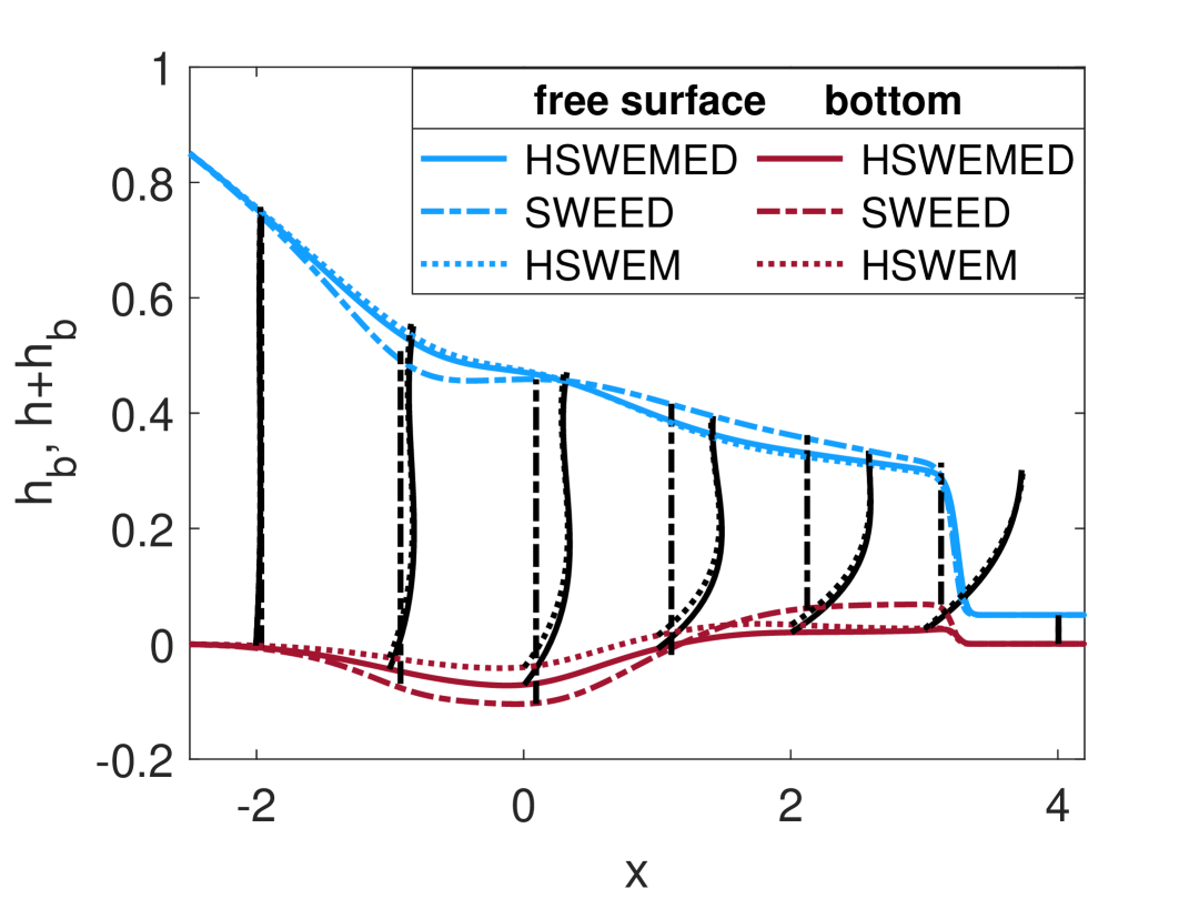
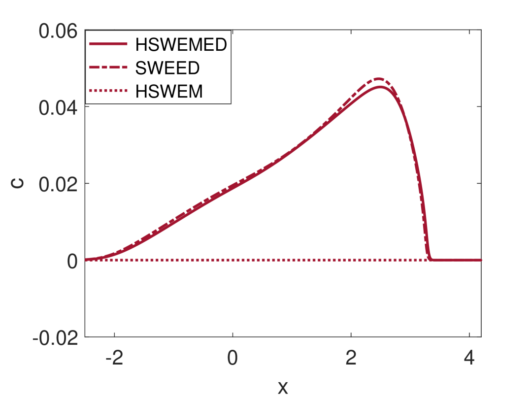
Figure 4: Academic dam-break: (Left) Free surface $h+h_{b}$ & sediment bottom evolution $h_{b}$, and vertical profiles of velocity $u$ (black lines) at model points $x=-2,\,-1,\,0,\,1,\,2,\,3$ and (right) volumetric sediment concentration $c$ in the suspension at $t=1,$ computed with the HSWEMED (solid), the SWEED (dash-dotted), and the HSWEM (dotted).

Figure 4 (left) indicates that the free surface $h+h_{b},$ and sediment bottom evolution $h_{b},$ predicted by the HSWEMED differ from those of the other two models. Specifically, when examining bottom evolution $h_{b}$, the HSWEMED predicts more erosion than the HSWEM and less erosion than the SWEED at the dam-break location. Furthermore, a significant fraction of the sediment remains suspended further upstream. This improvement comes from incorporating bottom velocity $u_{b}$ (28), which is lower than the depth-averaged velocity $u_{m}$ used in the SWEED. As expected, the SWEED tends to overestimate erosion, which explains its smaller $h_{b}$ around $x=0$ in the erosion domain. In contrast, the HSWEM only accounts for bedload transport without considering erosion and deposition effects, resulting in an inaccurate representation of bottom changes [24]. The lack of erosion and deposition modeling in the HSWEM leads to underestimating eroded material and has the largest $h_{b}$ around $x=0.$ Our proposed HSWEMED falls between the two, capturing a moderate level of erosion leading to reduced bedload transport. Regarding the free surface evolution $h+h_{b}$, the HSWEMED exhibits slight deviations near the wavefront, with less sediment exchange compared to the SWEED. As expected, the SWEED uses the depth-averaged velocity $u_{m}$ for the erosion, while the HSWEMED uses the bottom velocity $u_{b}$ (28) (which is smaller than $u_{m}$). This is also shown in Figure 4 (left), where we present the vertical profiles of velocity $u$ (21) at different points in the spatial direction. We see that our HSWEMED recovers the parabolic shape of the velocity, especially close to the front, and the bottom velocity computed with the HSWEMED is smaller than that of the HSWEM and the depth-averaged velocity used in the SWEED. However, it shows almost no difference when compared with the HSWEM, suggesting that erosion and deposition do not significantly influence the leading edge of the wave. The reason could be related to the minimal sediment exchange at the wavefront. Consequently, both the HSWEMED and HSWEM yield nearly identical results in this regard.

Figure 4 (right) illustrates the volumetric sediment concentration $c$ in the suspension for all three models. Since the HSWEM exclusively models bedload transport, it does not include sediment concentration in the suspension. Although both the HSWEMED and SWEED share the same settling velocity $\omega_{o}$, as defined in (39), the SWEED yields a slightly higher suspended sediment concentration than our proposed model. This discrepancy arises because the SWEED induces more sediment erosion near the dam-break location (around $x=0$) due to using the depth-averaged velocity.

4.2 Laboratory experiments: Simulation of dam-break flow over erodible sediment bed

In this section, we simulate one-dimensional dam-break flow over an erodible sediment bed and compare our HSWEMED model results with laboratory experiments documented in [44]. We analyze the free surface $h+h_{b}$, sediment bottom evolution $h_{b}$, and volumetric sediment concentration $c$ for three different initial configurations of water and sediment depths at upstream and downstream

• config 1: Dam-break flow with wet/dry front over flat bottom (same as config a in [44])

• config 2: Dam-break flow with wet/dry front over discontinuous bottom (same as config d in [44])

• config 3: Dam-break flow over discontinuous bottom with water at rest in the downstream (same as config f in [44])

For all three configurations, two different sediment bed materials are used: PVC pellets and uniform coarse sand with different densities to analyze how sediment density and transport properties affect the propagation speeds, sediment concentrations in suspension, and erosion processes. The properties of the bed materials are taken from [44] and shown in Table 3.

Materials	$\rho$	$\rho_{s}$	$\theta_{c}$	$\psi$	$d_{s}$	$\epsilon$
PVC	1000	1580	0.047	0.47	3.9	0.0324
Sand	1000	2683	0.047	0.47	1.82	0.0104

Table 3: Physical parameters of laboratory experiments.

4.2.1 Config 1: Dam-break flow with wet/dry front over flat bottom

For the first configuration, we use the following initial conditions for the water height $h,$ and sediment bed $h_{b}$

$$\vbox{\hbox{\shortstack{\includegraphics[width=173.44534pt]{IC_exp_1} \\ \small Figure 5: Initial water height and bottom\\ (config a in \cite[cite]{[\@@bibref{Number}{Spinewine01122007}{}{}]})}}}\qquad\begin{aligned} &h(0,x)=\begin{cases}0.35,&\quad\text{if $x\leq 0,$}\\ 0,&\quad\text{otherwise.}\end{cases}\\ &h_{b}(0,x)=0.\end{aligned}$$ (config 1)

The computational domain $\Omega=[-3,3]$ is divided into $N_{x}=1000$ grid points. Within this framework, we apply a wet/dry treatment in the HSWEMED by considering a computational cell as dry when the water height $h$ falls below a specified threshold, specifically when $h<\delta,$ with $\delta=10^{-4}$, to maintain numerical stability.

We consider the first-order HSWEMED in this configuration, i.e., $N=1$. In near-dry regions, where the water height $h$ is nearly zero, the friction term in the momentum equation (27) and the higher-order averaged equation (29) becomes excessively large due to the presence of $h$ in the denominator. Such behavior introduces significant numerical stiffness, leading to instability unless extremely small time steps are considered. Therefore, incorporating higher-order moments poses computational challenges. We defer this to future research, where an asymptotic-preserving numerical scheme could be applied, for example, using projective integration [2] or a time-splitting scheme [28].

For now, Figure 6 (left) and (right) present the numerical results for the free surface $h+h_{b}$ and bottom evolution $h_{b}$ at $t=1$, as computed by the first-order HSWEMED, the SWEED, and the first-order HSWEM. These results are compared with experimental data for PVC and coarser sand beds from [44]. Figure 6 (bottom) shows the PVC and sand bed sediment concentration $c$ at time $t=1$, computed with the HSWEMED and SWEED, since HSWEM only models bedload transport. Based on the figures, we draw three key observations: first, regarding the PVC bed; second, regarding the sand bed; and third, related to the volumetric sediment concentration in suspension for both PVC pellets and sand particles.

For the PVC bed, Figure 6 (left) demonstrates that the sediment entrainment predicted by the HSWEMED, both upstream and downstream, aligns more closely with experimental data compared to the other two models. Specifically, the SWEED overestimates bottom erosion in the dam-break region. The difference in results between the HSWEMED and SWEED can be associated with the differences in bottom velocity $u_{b}$. The erosion rate and sediment transport in the HSWEMED are computed using a velocity $u_{b}=u_{m}+\displaystyle\sum_{j=1}^{N}\alpha_{j}$, which is lower than the depth-averaged velocity $u_{b}=u_{m}$, estimated by the SWEED. In contrast, only slight differences are observed when compared to the HSWEM, which neglects the effects of erosion at the bottom and only models bedload transport. Additionally, the HSWEMED accurately captures the location of the hydraulic jump at $x=0$, although it does not perfectly reproduce the experimental free surface in this region. Nonetheless, the HSWEMED outperforms both SWEED and HSWEM.

For the sand bed, Figure 6 (right) shows that the HSWEMED effectively simulates both the upstream sediment entrainment and the downstream free surface, outperforming the SWEED and HSWEM. The SWEED slightly overestimates erosion near the dam-break region at $x=0$, whereas the HSWEM slightly underestimates it. This underestimation occurs because the HSWEM does not include the source terms associated with erosion and deposition in the momentum and higher-order averaged equations. Furthermore, sediment erosion, transport, and bed changes are less pronounced for sand particles than for PVC pellets, due to the higher density of sand. Focusing on the wavefront advancement for both PVC and sand at $t=1$ indicates that the fast propagation of the sand wavefront is associated with shallower water depths along the wave, as PVC pellets are being less resistant to water flow, leading to higher water depths downstream. The HSWEMED effectively captures these overall dynamics.

For the volumetric sediment concentration $c$, Figure 6 (bottom) illustrates that the sediment concentration in suspension is higher for PVC pellets than for sand particles, as computed by both the HSWEMED and the SWEED. The difference in suspended sediment is associated with the lower specific gravity or density of PVC pellets ($\rho_{s}/\rho_{w}\approx 1.5$) compared to sand particles ($\rho_{s}/\rho_{w}\approx 2.6$). Under the same hydraulic conditions, the settling velocity for PVC pellets $(\omega_{o}=0.1528)$, computed from equation (39), is lower than that of sand particles $(\omega_{o}=0.5714)$. The lower density and slower settling velocity allow PVC particles to remain suspended longer than sand particles, leading to a broader and smoother concentration profile for the PVC bed. In addition, the lower sediment concentration in the suspension zone affects the wavefront propagation speed for PVC pellets. For example, near $x\approx 1.6$, the suspended sediment concentration for PVC pellets computed using the HSWEMED reaches its maximum value, $c\approx 0.05$. In contrast, the corresponding concentration for sand at the same location is approximately $c\approx 0.04$. By comparing the propagation speed at this location for both materials through the second factor of the characteristic polynomial discussed in equation (60), it is evident in Table 4 that the characteristic speed of sand particles is greater than that of PVC pellets, as expected. This observation also explains the faster propagation of the wavefront for sand particles seen in Figure 6 (right).

Furthermore, when comparing the sediment concentration computed by the HSWEMED and SWEED, we observe that the SWEED shows more sediment in suspension than the HSWEMED. This is expected, as the SWEED tends to overestimate bottom erosion, which ultimately contributes to higher concentrations in the suspension zone.

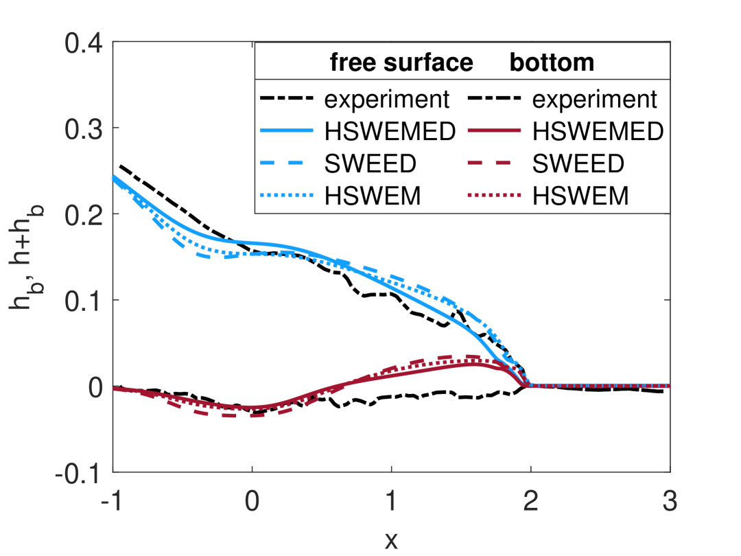
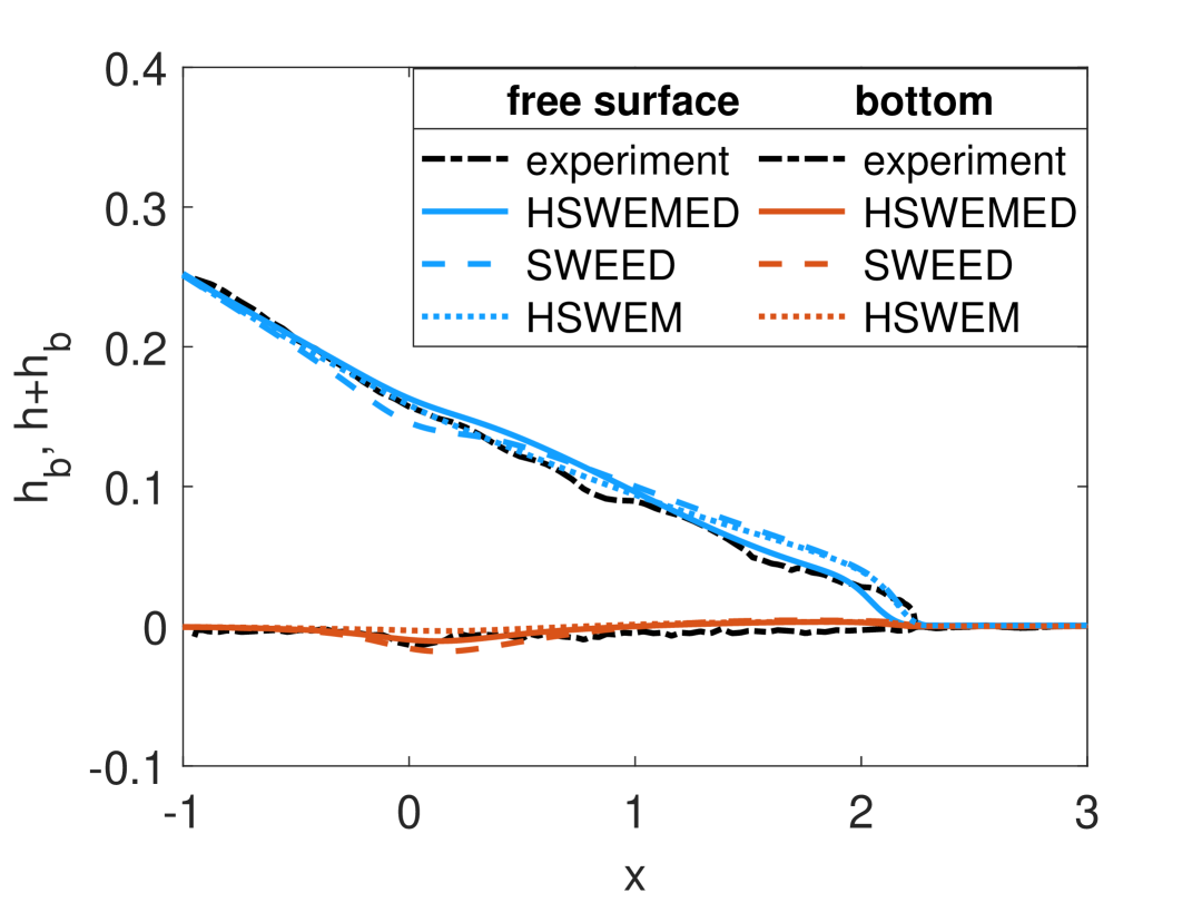
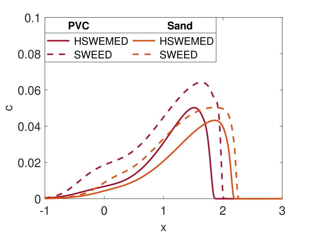
Figure 6: config 1: Free surface & bottom evolution at time $t=1$ computed with the HSWEMED (solid), the SWEED (dashed), and the HSWEM (dotted). Results are compared with experimental data (dash-dotted) for the bed materials (left) PVC pellets and (right) uniform coarse sand. (bottom) Volumetric sediment concentration in the suspension at $t=1,$ computed with HSWEMED (solid) and the SWEED (dashed) for PVC and sand bed.

Characteristic speed	PVC	Sand
$\lambda_{1}$	$-0.4350$	$-0.0619$
$\lambda_{2}$	$1.0148$	$1.0786$
$\lambda_{3}$	$1.8333$	$2.4437$

Table 4: The characteristic speed, computed around $x\approx 1.6$ at time $t=1$ from the second factor of (60) using the HSWEMED model for the PVC and sand bed under config 1, shows that the maximum speeds are higher for sand particles compared to PVC.

4.2.2 Config 2: Dam-break flow with wet/dry front over discontinuous bottom

For the second configuration, the initial water height $h,$ and the sediment bed $h_{b}$ are given by

$$\vbox{\hbox{\shortstack{\includegraphics[width=173.44534pt]{IC_exp_2} \\ \small Figure 7: Initial water height and bottom \\ (config d in \cite[cite]{[\@@bibref{Number}{Spinewine01122007}{}{}]})}}}\quad\begin{aligned} \qquad&h(0,x)=\begin{cases}0.25,&\quad\text{if $x\leq 0,$}\\ 0,&\quad\text{otherwise.}\end{cases}\\ &h_{b}(0,x)=\begin{cases}0.10,&\quad\text{if $x\leq 0,$}\\ 0,&\quad\text{otherwise.}\end{cases}\end{aligned}$$ (config 2)

The primary difference in this configuration compared to the first is the presence of a discontinuous bottom $h_{b}$.

We consider $\Omega=[-3,3]$ as the computational domain [44], discretized into $N_{x}=1000$ equally spaced points. Similar to the first configuration, we consider the order of moments, $N=1$, and implement a wet/dry front treatment to ensure numerical stability.

Figure 8 (left) and (right) present the numerical results for the free surface $h+h_{b},$ and bottom evolution $h_{b}$ at $t=1$, as computed by the first-order HSWEMED, the SWEED, and the first-order HSWEM. Like the previous configuration, we compare the model results with experimental data for PVC and coarser sand bed from [44]. Figure 8 (bottom) illustrates the sediment concentration $c$ for both bed materials at time $t=1$ computed with the HSWEMED and SWEED. Based on the figures, we again draw three key observations: First, regarding the PVC bed; second, regarding the sand bed; and third, related to the volumetric sediment concentration in suspension for both PVC pellets and sand particles.

For the PVC bed, Figure 8 (left) shows that the proposed HSWEMED exhibits better agreement with experimental data than the SWEED and HSWEM, particularly in capturing the wavefront and the location of the hydraulic jump at $x=0$. In contrast, the SWEED and HSWEM fail to reproduce the jump, with the computed position of the wavefront consistently ahead of the experimental data. Furthermore, sediment entrainment at the bottom, as predicted by the HSWEMED, aligns more closely with measurements than the other models, though some discrepancies remain. These deviations can be attributed to the same factors as in the first configuration: in the SWEED, the average bottom velocity leads to higher friction, erosion rates, and sediment transport, while in the HSWEM, the absence of erosion and deposition effects may result in underestimating sediment dynamics.

For the sand bed, Figure 8 (right) demonstrates that the HSWEMED accurately reproduces the upstream and downstream free surface, wavefront, and bottom sediment evolution, showing excellent agreement with the experimental data. However, when comparing the HSWEMED with the SWEED and HSWEM, no significant differences are observed among the three models. This similarity suggests that erosion and deposition effects are minimal for coarser particles, leading to comparable predictions across all models.

For the sediment concentration $c$, Figure 8 (bottom) demonstrates that the PVC bed shows a broader spatial expansion than the sand bed, both upstream and downstream of the peak of concentration as computed by both the HSWEMED and the SWEED. The difference in suspended sediments for PVC and sand particles can be associated with the physical properties of the bed materials. As mentioned in Table 3, PVC pellets with a lower density, larger particle size, and lower settling velocity are able to stay in suspension for an extended period before settling. In contrast, the sand particles with higher density and faster settling velocity form a narrower and sharper concentration profile. When comparing the concentration of the HSWEMED and the SWEED, we observe that the SWEED exhibits a higher sediment concentration in suspension and an extensive spatial distribution compared to the HSWEMED. The result is what we expect and is consistent with the explanation provided in Section 4.2.1.

Furthermore, it is important to emphasize that sharply descending, discontinuous bed profiles with wet/dry fronts pose significant numerical challenges. Despite these challenges, the coupled HSWEMED effectively captures the key dynamics for both bed materials, including the hydraulic jump in the free surface around $x=0.$

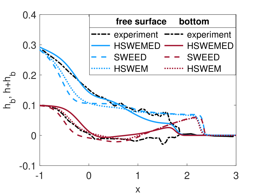
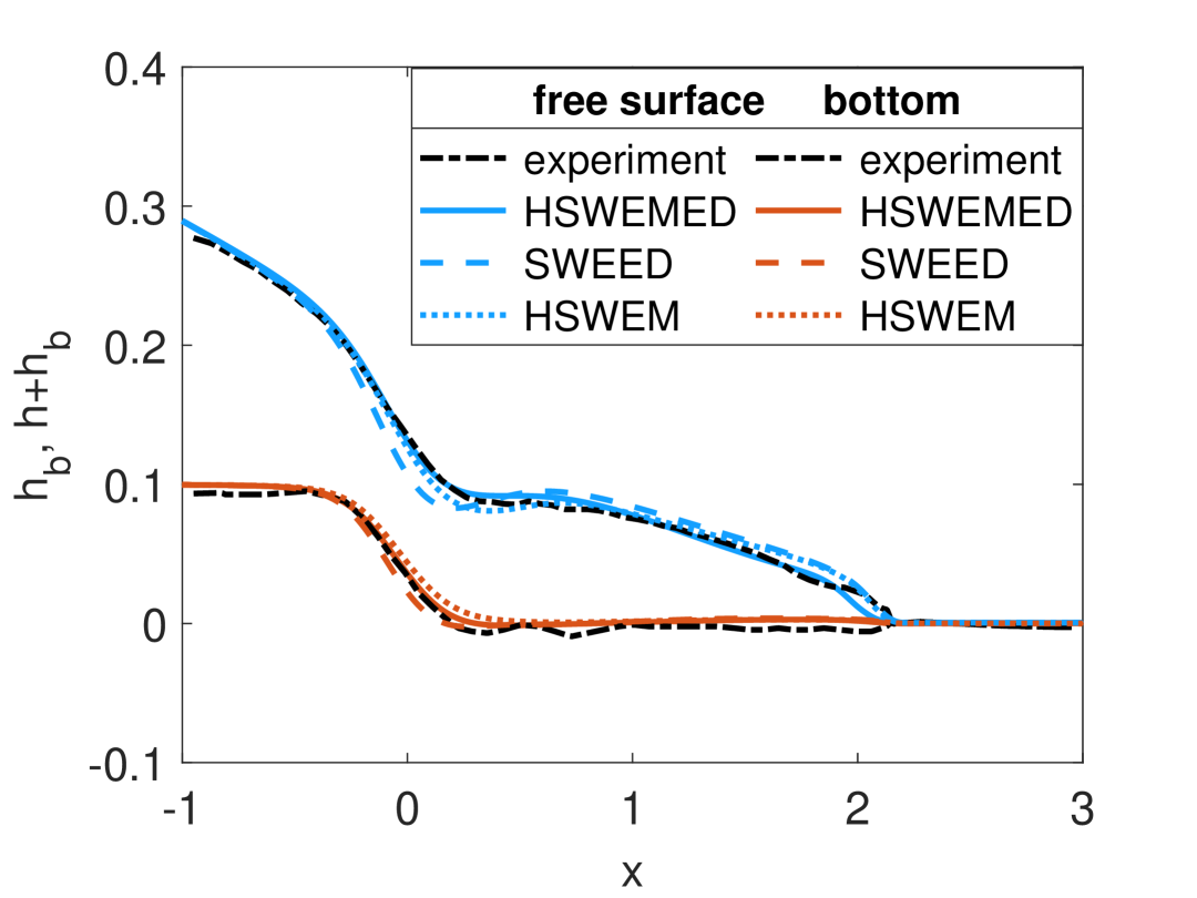
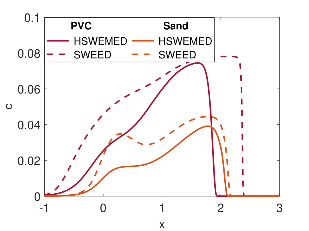
Figure 8: config 2: Free surface & bottom evolution at time $t=1$ computed with the HSWEMED (solid), the SWEED (dashed), and the HSWEM (dotted). Results are compared with experimental data (dash-dotted) for the bed materials (left) PVC pellets and (right) uniform coarse sand. (bottom) Volumetric sediment concentration in the suspension at $t=1,$ computed with the HSWEMED (solid) and the SWEED (dashed) for PVC and sand bed.

4.2.3 Config 3: Dam-break flow over discontinuous bottom with water in the downstream

For the third configuration, the initial water height $h,$ and the sediment bed $h_{b}$ are given by

$$\vbox{\hbox{\shortstack{\includegraphics[width=173.44534pt]{IC_exp_3} \\ \small Figure 9: Initial water height and bottom \\ (config f in \cite[cite]{[\@@bibref{Number}{Spinewine01122007}{}{}]})}}}\quad\begin{aligned} \qquad&h(0,x)=\begin{cases}0.25,&\quad\text{if $x\leq 0,$}\\ 0.10,&\quad\text{otherwise.}\end{cases}\\ &h_{b}(0,x)=\begin{cases}0.10,&\quad\text{if $x\leq 0,$}\\ 0,&\quad\text{otherwise.}\end{cases}\end{aligned}$$ (config 3)

We consider $\Omega=[-3,3]$ as the computational domain, discretized into $N_{x}=1000$ equally spaced points. The main difference in this setup, compared to the first and second configurations, is the presence of a wet downstream.

In this test case, we again consider the third-order HSWEMED, i.e., $N=3$, and this choice is consistent with the value of $N$ used for the HSWEM in [24], whose results are comparedwith those of the HSWEMED.

Figure 10 (left) and (right) present the numerical results for the free surface $h+h_{b},$ and bottom evolution $h_{b}$ at $t=1$, as computed by the third-order HSWEMED, the SWEED, and the third-order HSWEM models. We compare the model results with experimental data for PVC and coarser sand beds. Figure 10 (bottom) illustrates the sediment concentration $c$ for both bed materials at time $t=1$ computed with the HSWEMED and SWEED. From the figures, we again draw the following three observations: First, regarding the PVC bed; second, regarding the sand bed; and third, related to the volumetric sediment concentration in suspension for both PVC pellets and sand particles.

For the PVC bed, Figure 10 (left) illustrates that the free surface $h+h_{b},$ in the vicinity of the hydraulic jump, occurring at $x=0$ is only partially captured by the three models. This discrepancy arises from a deviation between the experimentally observed and computationally predicted positions of the free surface. The difference could be attributed to the limitations of the shallow water model assumptions, as it does not account for non-hydrostatic pressure, especially near the location of the dam-break. However, the models accurately reproduce the advancement of the waterfront and downstream bed evolution. The analysis indicates that the three models yield consistent results across the computational domain, except in the region near the hydraulic jump $x=0$, where minor discrepancies are observed.

For the sand bed, Figure 10 (right) demonstrates that the free surface $h+h_{b},$ in the region of the hydraulic jump around $x=0$ is only partially captured by the three models, similar to the observations for the PVC bed. However, the propagation of the waterfront is well aligned with the experimental data, indicating a high level of agreement. Furthermore, the sediment distribution at upstream and downstream locations, as well as the sharp variations in bed changes $h_{b}$, are successfully captured by the models. However, we do not observe any significant differences among the three models. The similarities can be related to the low friction coefficient $(\epsilon=0.0104\,\,\text{for sand})$ used in this experiment, which does not generate significant differences between the model results. This is shown in Figure 11 (left), which is generated using an approximately three times larger friction coefficient for sand particles, we notice some differences in free surface and bed evolution between the HSWEMED and the SWEED, particularly around $x=0$, where the Froude number $(u_{m}/\sqrt{gh})$ is relatively high as shown in Figure 11 (right) similar to [24]. Moreover, in Figure 11 (left), we present the vertical profiles of the velocity at different locations in the spatial directions. It is observed that the vertical structures of the velocity profiles are evident when $x\in[0,1],$ and for the rest of the domain, the vertical profiles are very close to the depth-averaged velocity. A similar scenario was also analyzed in [24]. Note that we do not present the velocity profile for the first and second configuration of laboratory experiments, as we only consider the linear velocity profiles with $N=1$ due to the potential stiffness at the wet/dry fronts.

For the sediment concentration $c$, Figure 10 (bottom) illustrates that the peak of the sediment concentration and spatial expansion for the PVC bed are higher than those for the sand bed. The difference in concentration computed by the HSWEMED and SWEED is related to the difference in density, settling velocity, and the low friction considered in this experiment for sand particles, as also explained in Section 4.2.1 and Section 4.2.2.

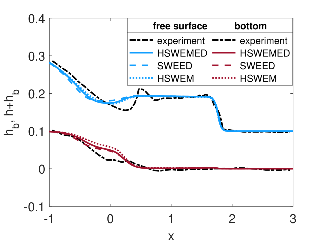
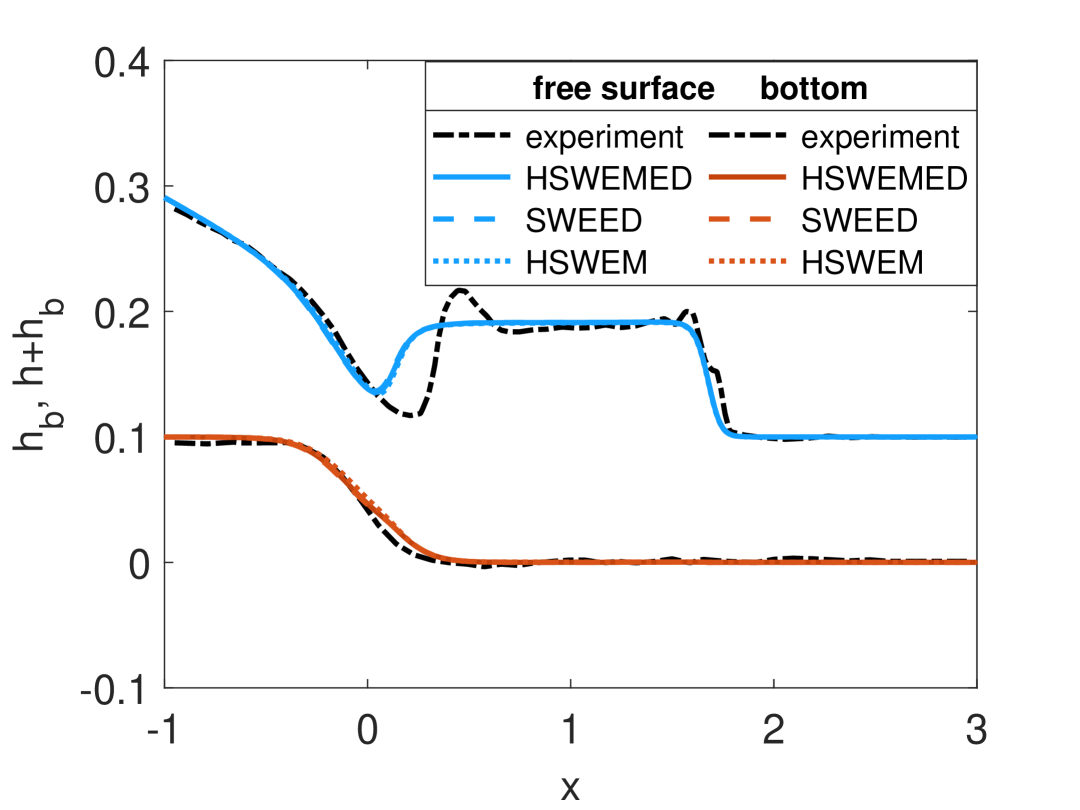
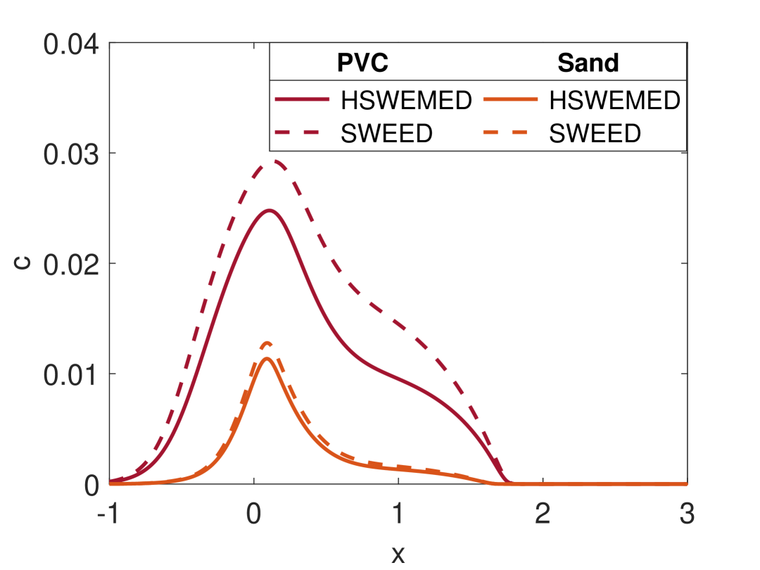
Figure 10: config 3: Free surface & bottom evolution at time $t=1$ computed with the HSWEMED (solid), the SWEED (dashed), and the HSWEM (dotted). Results are compared with experimental data (dash-dotted) for the bed materials (left) PVC pellets and (right) uniform coarse sand. (bottom) Volumetric sediment concentration for PVC (solid) and sand (dashed) bed at time $t=1$ computed with the HSWEMED and the SWEED.

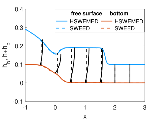
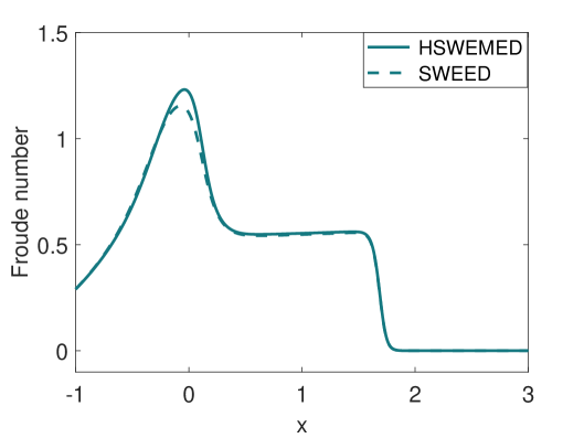
Figure 11: For a sand bed with config 3, dam-break simulations at time $t=1$ with increasing friction coefficient $\epsilon=0.0324$; (left) free surface, bottom evolution, and vertical profiles of velocity at $x=-0.5,0.0,0.5,1.0,1.5,2.0,2.5,$ computed with the HSWEMED (black solid) and the SWEED (black dashed), (right) Froude number, computed with the HSWEMED (solid) and the SWEED (dashed).

5 Conclusion

We developed a comprehensive one-dimensional coupled hydro-morphodynamic model to simulate sediment transport, incorporating bedload and suspended load dynamics with vertical velocity variations. The model is based on the shallow water moment framework, which governs the flow hydrodynamics, volumetric sediment concentration, and morphological evolution through the Exner equation. Using the moment approach allows us to recover the vertical structure of the horizontal velocity of the fluid, thereby accurately approximating the velocity close to the bottom. The bottom velocity is crucial, as its accurate approximation influences sediment discharge and erosion rates, thereby, the bedload and suspended load transport. To close the system, we integrated the Meyer-Peter & Müller formula for sediment discharge, empirical laws for erosion and deposition, non-linear Manning friction for bed resistance, and Newtonian friction to represent fluid shear stresses.

Recognizing that the classical Shallow Water Moment model (SWM) loses hyperbolicity at higher-order moments, i.e., $N\geq 2$, we adopted the regularization technique introduced in [31] to derive a Hyperbolic Shallow Water Exner Moment model accounting for Erosion and Deposition, referred to as HSWEMED. We showed the hyperbolicity of the proposed model by analytically deriving and analyzing the characteristic polynomial of the governing matrix and comparing it with the characteristic polynomials of the HSWEM and the SWEED, which are hyperbolic themselves. Our primary finding is that integrating the regularized moment approach with erosion and deposition effects preserves the hyperbolicity of the overall model.

In the numerical simulation of a dam-break test case, the HSWEMED produced a more realistic shape of bottom evolution than the SWEED and the HSWEM. This improvement is associated with the better approximation of bottom velocity and its explicit incorporation of erosion and deposition processes. Additionally, we compared the HSWEMED results (free surface and bottom evolution) with laboratory experiments from the literature [44] for three dam-break configurations using two different bed materials: PVC and uniform coarse sand. The results showed good agreement between the HSWEMED and experimental data. When comparing the HSWEMED results with those of the SWEED and HSWEM, differences were observed for the lighter PVC particles, while the heavier sand particles led to smaller differences. This behavior is related to the low bed friction coefficient used in the sand laboratory experiments, which cannot generate a vertical velocity structure during these rapid and short-time simulations. As observed in the third configuration case, the difference is noticeable for increased friction coefficients, especially in the region where the Froude number is also significant. The HSWEM only models bedload transport and fails to produce the bed changes accurately due to the omission of erosion and deposition effects at the sediment bed. We also compared the volumetric sediment concentration profiles in the suspension zone obtained from the HSWEMED for both PVC and sand beds. The results showed that sand particles settle more rapidly than PVC pellets, which is related to the higher density and, consequently, greater settling velocity of sand.

Ongoing work is directed toward conducting equilibrium stability and steady-state analyses of the HSWEMED. Future works will focus on extending the model by applying a polynomial expansion to the sediment concentration profile and performing complex test cases. Another interest for future work will be using a well-balanced or positivity-preserving numerical scheme that can address the challenges of using higher-order moments, particularly in wet/dry fronts.

Appendices

Appendix A Derivation of the complete reference system

A.1 Mapping of the mass balance

From the divergence-free conditions $\nabla\cdot\mathbf{u}=0$, we have

$$\partial_{x}u+\partial_{z}w=0.$$ (63)

After multiplying (63) by $h$ and applying the differential operator (15), the mapped mass balance yields

$$\partial_{x}\left(h\tilde{u}\right)-\partial_{\zeta}\left[\partial_{x}(\zeta h+h_{b})\tilde{u}\right]+\partial_{\zeta}\tilde{w}=0.$$ (64)

A.2 Mapping of the momentum balance

From the reference system (7),

$$\partial_{t}u+\partial_{x}u^{2}+\partial_{z}(uw)=-\frac{1}{\rho}\partial_{x}p+\frac{1}{\rho}\partial_{z}\sigma_{xz}.$$ (65)

After multiplying (65) by $h$ and applying the differential operator (15), the mapped momentum balance yields

$$\begin{split}\partial_{t}(h\tilde{u})-\partial_{\zeta}\left(\tilde{u}\partial_{t}\left(\zeta h+h_{b}\right)\right)&+\partial_{x}(h\tilde{u}^{2})-\partial_{\zeta}\left(\tilde{u}^{2}\partial_{x}\left(\zeta h+h_{b}\right)\right)+\partial_{\zeta}(\tilde{u}\tilde{w})\\ &+\frac{1}{\rho}\partial_{x}(h\tilde{p})-\frac{1}{\rho}\partial_{\zeta}\left(\tilde{p}\partial_{x}(\zeta h+h_{b})\right)=\frac{1}{\rho}\partial_{\zeta}\tilde{\sigma}_{xz},\end{split}$$ (66)

$$\begin{split}\Longrightarrow\partial_{t}(h\tilde{u})+\partial_{x}(h\tilde{u}^{2})+&\partial_{\zeta}\left[\tilde{u}\left(\underbrace{\tilde{w}-\tilde{u}\partial_{x}\left(\zeta h+h_{b}\right)-\partial_{t}\left(\zeta h+h_{b}\right)}_{\text{vertical coupling}}\right)\right]\\ &+\underbrace{\frac{1}{\rho}\partial_{x}(h\tilde{p})-\frac{1}{\rho}\partial_{\zeta}\left(\tilde{p}\partial_{x}(\zeta h+h_{b})\right)}_{\text{pressure}}=\frac{1}{\rho}\partial_{\zeta}\tilde{\sigma}_{xz}.\end{split}$$ (67)

From the hydrostatic balance, we have $p(t,x,z)=(h_{s}-z)\rho g$. After mapping from $z$ to $\zeta$ we get

$$p(t,x,\zeta)=(h_{s}-(\zeta h+h_{b}))\rho g=h(1-\zeta)\rho g.$$ (68)

Therefore,

$$\frac{1}{\rho}\partial_{x}(h\tilde{p})-\frac{1}{\rho}\partial_{\zeta}\left(\tilde{p}\partial_{x}(\zeta h+h_{b})\right) =\frac{1}{\rho}\partial_{x}\left(\rho gh^{2}(1-\zeta)\right)-\frac{1}{\rho}\partial_{\zeta}\left(\rho gh(1-\zeta)\partial_{x}(\zeta h+h_{b})\right)$$

$$=2g(1-\zeta)h\partial_{x}h+\frac{gh^{2}}{\rho}(1-\zeta)\partial_{x}\rho-\left(gh\partial_{x}h-2gh\zeta\partial_{x}h-gh\partial_{x}h_{b}\right)$$

$$=gh\partial_{x}h+gh\partial_{x}h_{b}+\frac{gh^{2}}{\rho}(1-\zeta)\partial_{x}\rho.$$ (69)

Now we substitute (A.2) to (67)

$$\partial_{t}(h\tilde{u})+\partial_{x}(h\tilde{u}^{2})+\partial_{\zeta}\left[\tilde{u}\left(\tilde{w}-\tilde{u}\partial_{x}\left(\zeta h+h_{b}\right)-\partial_{t}\left(\zeta h+h_{b}\right)\right)\right]+gh\partial_{x}(h+h_{b})+\frac{gh^{2}}{\rho}(1-\zeta)\partial_{x}\rho=\frac{1}{\rho}\partial_{\zeta}\tilde{\sigma}_{xz}.$$ (70)

A.3 Mapping of the sediment concentration equation

From the reference system (8), we have

$$\partial_{t}c+\partial_{x}(cu)+\partial_{z}(cw)=0.$$ (71)

After multiplying (71) by $h$ and applying the differential operator (15), the mapped sediment concentration equation yields

$$\partial_{t}(h\tilde{c})+\partial_{x}\left(h\tilde{c}\tilde{u}\right)+\partial_{\zeta}\left[\tilde{c}\left(\tilde{w}-\partial_{x}(\zeta h+h_{b})\tilde{u}-\partial_{t}(\zeta h+h_{b})\right)\right]=0.$$ (72)

Appendix B Averages of the Horizontal Momentum Balances

B.1 Depth-averaging the momentum balance

We consider the momentum balance (17) and after integrating $\int_{0}^{1}\cdot\,d\zeta$, we get

$$\begin{split}\int_{0}^{1}\partial_{t}(h\tilde{u})\,d\zeta&+\int_{0}^{1}\partial_{x}(h\tilde{u}^{2})\,d\zeta+\int_{0}^{1}\partial_{\zeta}\left[\tilde{u}\left(\tilde{w}-\tilde{u}\partial_{x}\left(\zeta h+h_{b}\right)-\partial_{t}\left(\zeta h+h_{b}\right)\right)\right]\,d\zeta\\ &+\int_{0}^{1}gh\partial_{x}h\,d\zeta+\int_{0}^{1}gh\partial_{x}h_{b}\,d\zeta+\int_{0}^{1}\frac{gh^{2}}{\rho}(1-\zeta)\partial_{x}\rho\,\,d\zeta=\frac{1}{\rho}\int_{0}^{1}\partial_{\zeta}\tilde{\sigma}_{xz}\,d\zeta,\end{split}$$

$$\begin{split}\Rightarrow\partial_{t}\left(h\int_{0}^{1}\tilde{u}\,d\zeta\right)&+\partial_{x}\left(h\int_{0}^{1}\tilde{u}^{2}\,d\zeta\right)+\partial_{\zeta}\left(\int_{0}^{1}\tilde{u}\left(\tilde{w}-\tilde{u}\partial_{x}\left(\zeta h+h_{b}\right)-\partial_{t}\left(\zeta h+h_{b}\right)\right)\,d\zeta\right)\\ &+gh\partial_{x}h+gh\partial_{x}h_{b}+\frac{gh^{2}}{2\rho}\partial_{x}\rho=\frac{1}{\rho}\partial_{\zeta}\left(\int_{0}^{1}\tilde{\sigma}_{xz}\,d\zeta\right).\end{split}$$ (73)

After applying the kinematic boundary conditions (19)-(20) and substituting $\tilde{u}(t,x,\zeta)=u_{m}(t,x)+\sum_{j=1}^{N}\alpha_{j}(t,x)\,\phi_{j}(\zeta)$, we get

$$\begin{split}\partial_{t}(hu_{m})+\partial_{x}\left(hu_{m}^{2}+h\sum\frac{\alpha_{j}^{2}}{2j+1}+\frac{gh^{2}}{2}\right)=-gh\partial_{x}h_{b}-\frac{gh^{2}}{2\rho}(\rho_{s}-\rho_{w})\partial_{x}c+\frac{\phi_{b}u_{b}}{1-\psi}-\epsilon|u_{b}|u_{b}.\end{split}$$ (74)

Abbreviation of matrices
 
Here we introduce six matrices which are generated by the scaled Legendre polynomials

$$A_{ijk} =(2i+1)\int_{0}^{1}\phi_{i}\phi_{j}\phi_{k}\,d\zeta, \quad B_{ijk} =(2i+1)\int_{0}^{1}\phi_{i}^{\prime}\left(\phi_{j}d\hat{\zeta}\right)\phi_{k}\,d\zeta,$$

$$C_{ij} =\int_{0}^{1}\phi_{i}^{\prime}\phi_{j}^{\prime}\,d\zeta, \quad H_{ij} =(2i+1)\int_{0}^{1}\zeta\phi_{i}\phi_{j}^{\prime}\,d\zeta,$$

$$G_{ij} =(2i+1)\int_{0}^{1}\phi_{i}\phi_{j}^{\prime}\,d\zeta, \quad K_{i} =\int_{0}^{1}\zeta\phi_{i}\,d\zeta.$$

B.2 Higher-order averages in $x$

To get the higher-order averages, multiply (17) with the ansatz function $\phi_{i}(\zeta)$ and integrate from $\zeta=0$ to $\zeta=1$,

$$\begin{split}&\partial_{t}\left(h\int_{0}^{1}\phi_{i}\tilde{u}\,d\zeta\right)+\partial_{x}\left(h\int_{0}^{1}\phi_{i}\tilde{u}^{2}\,d\zeta\right)+gh\partial_{x}(h+h_{b})\int_{0}^{1}\phi_{i}\,d\zeta\\ &+\int_{0}^{1}\phi_{i}\partial_{\zeta}\left[\tilde{u}\left(\tilde{w}-\tilde{u}\partial_{x}\left(\zeta h+h_{b}\right)-\partial_{t}\left(\zeta h+h_{b}\right)\right)\right]\,d\zeta=-\frac{gh^{2}}{\rho}\partial_{x}\rho\int_{0}^{1}(1-\zeta)\phi_{i}\,\,d\zeta+\frac{1}{\rho}\int_{0}^{1}\phi_{i}\partial_{\zeta}\tilde{\sigma}_{xz}\,d\zeta.\end{split}$$ (75)

We have,

$$\int_{0}^{1}\phi_{i}\tilde{u}\,d\zeta =\int_{0}^{1}\phi_{i}\left(u_{m}+\sum_{j=1}^{N}\alpha_{j}\phi_{j}\right)\,d\zeta=\frac{\alpha_{i}}{2i+1}.$$ (76)

and

$$\int_{0}^{1}\phi_{i}\tilde{u}^{2}\,\,d\zeta =\int_{0}^{1}\phi_{i}\left(u_{m}^{2}+2u_{m}\sum_{j=1}^{N}\alpha_{j}\phi_{j}+\sum_{j=1}^{N}\alpha_{j}\phi_{j}\sum_{j=1}^{N}\alpha_{j}\phi_{j}\right)\,d\zeta=\frac{1}{2i+1}\left(2u_{m}\alpha_{i}+\sum_{j,k=1}^{N}\alpha_{j}\alpha_{k}A_{ijk}\right).$$ (77)

The projection on vertical coupling term reads

$$\int_{0}^{1}\phi_{i}\partial_{\zeta}\left[\tilde{u}\left(\tilde{w}-\tilde{u}\partial_{x}\left(\zeta h+h_{b}\right)-\partial_{t}\left(\zeta h+h_{b}\right)\right)\right]\,d\zeta$$

$$= \int_{0}^{1}\phi_{i}\partial_{\zeta}\left[\tilde{u}\left(-\partial_{x}\left(h\int_{0}^{\zeta}\tilde{u}d\hat{\zeta}\right)-\zeta\left(-\partial_{x}\left(hu_{m}\right)+\frac{F_{b}}{1-\psi}\right)-\partial_{t}\,h_{b}\right)\right]\,d\zeta$$

$$= \int_{0}^{1}\phi_{i}\partial_{\zeta}\left[\tilde{u}\left(\partial_{x}\left(h\int_{0}^{\zeta}(u_{m}-\tilde{u})\,d\hat{\zeta}\right)\right)\right]\,d\zeta-\int_{0}^{1}\phi_{i}\partial_{\zeta}\left(\tilde{u}\frac{\zeta F_{b}}{1-\psi}\right)\,d\zeta-\int_{0}^{1}\phi_{i}\partial_{\zeta}\left(\tilde{u}\partial_{t}h_{b}\right)d\zeta$$

$$= -\int_{0}^{1}\phi_{i}\partial_{\zeta}\left[\tilde{u}\left(\partial_{x}\left(h\int_{0}^{\zeta}u_{d}\,d\hat{\zeta}\right)\right)\right]\,d\zeta-\frac{F_{b}}{1-\psi}\int_{0}^{1}\phi_{i}\partial_{\zeta}\left(\tilde{u}\zeta\right)\,d\zeta-\partial_{t}h_{b}\int_{0}^{1}\phi_{i}\partial_{\zeta}\tilde{u}\,d\zeta.$$ (78)

We notice the presence of the integral associated with erosion and deposition

$$\frac{F_{b}}{1-\psi}\int_{0}^{1}\phi_{i}\partial_{\zeta}\left(\tilde{u}\zeta\right)\,d\zeta=\frac{F_{b}}{1-\psi}\left(\sum_{j=1}^{N}\int_{0}^{1}\alpha_{j}\phi_{i}\phi_{j}\,d\zeta+\sum_{j=1}^{N}\int_{0}^{1}\alpha_{j}\zeta\phi_{i}\phi_{j}^{\prime}\,d\zeta\right)=\frac{F_{b}}{1-\psi}\left(\frac{\alpha_{i}}{2i+1}+\frac{\sum_{j=1}^{N}\alpha_{j}H_{ij}}{2i+1}\right).$$ (79)

and the projection related to the coupling with the bed evolution

$$\partial_{t}h_{b}\int_{0}^{1}\phi_{i}\partial_{\zeta}\tilde{u}\,d\zeta=\partial_{t}h_{b}\sum_{j=1}^{N}\alpha_{j}\left(\int_{0}^{1}\phi_{i}\phi_{j}^{\prime}\,d\zeta\right)=\partial_{t}h_{b}\frac{\sum_{j=1}^{N}\alpha_{j}G_{ij}}{2i+1}.$$ (80)

Therefore, the projection of the vertical coupling for higher-order reads

$$\int_{0}^{1}\phi_{i}\partial_{\zeta} \left[\tilde{u}\left(\tilde{w}-\tilde{u}\partial_{x}\left(\zeta h+h_{b}\right)-\partial_{t}\left(\zeta h+h_{b}\right)\right)\right]\,d\zeta=-\frac{u_{m}}{2i+1}\partial_{x}(h\alpha_{i})+\frac{1}{2i+1}\sum_{j,k=1}^{N}B_{ijk}\alpha_{k}\partial_{x}(h\alpha_{j})$$

$$-\frac{1}{2i+1}\frac{F_{b}}{1-\psi}\left(\alpha_{i}+\sum_{j=1}^{N}\alpha_{j}(H_{ij}-G_{ij})\right)+\frac{1}{2i+1}\sum_{j=1}^{N}\alpha_{j}G_{ij}\partial_{x}\frac{Q_{b}}{1-\psi}.$$ (81)

Similarly, we integrate the term that accounts for density variation

$$\frac{gh^{2}}{\rho}\frac{\partial\rho}{\partial x}\int_{0}^{1}(1-\zeta)\phi_{i}\,d\zeta=\frac{gh^{2}}{\rho}(\rho_{s}-\rho_{w})\frac{\partial c}{\partial x}\left(-\int_{0}^{1}\zeta\phi_{i}\,d\zeta\right)=-\frac{gh^{2}}{\rho}(\rho_{s}-\rho_{w})\frac{\partial c}{\partial x}K_{i}.$$ (82)

and the friction term for the additional moment equations,

$$\frac{1}{\rho}\int_{0}^{1}\phi_{i}\partial_{\zeta}\sigma_{xz}\,d\zeta=\frac{1}{\rho}\int_{0}^{1}\partial_{\zeta}(\phi_{i}\sigma_{xz})\,d\zeta-\frac{1}{\rho}\int_{0}^{1}\sigma_{xz}\partial_{\zeta}\phi_{i}\,d\zeta =-\epsilon|u_{b}|u_{b}-\frac{\nu}{h}\sum_{j=1}^{N}\int_{0}^{1}\alpha_{j}\phi_{i}^{\prime}\phi_{j}^{\prime}\,d\zeta$$

$$=-\epsilon|u_{b}|u_{b}-\frac{\nu}{h}\sum_{j=1}^{N}\alpha_{j}C_{ij}.$$ (83)

After putting all together, we obtain the higher average momentum balance in $x$ direction

$$\begin{split}&\partial_{t}(h\alpha_{i})+\partial_{x}\left(2hu_{m}\alpha_{i}+h\sum_{j,k=1}^{N}\alpha_{j}\alpha_{k}A_{ijk}\right)=u_{m}\partial_{x}(h\alpha_{i})-\sum_{j,k=1}^{N}B_{ijk}\alpha_{k}\partial_{x}(h\alpha_{j})\\ &+\frac{F_{b}}{1-\psi}\left(\alpha_{i}+\sum_{j=1}^{N}\alpha_{j}(H_{ij}-G_{ij})\right)-\sum_{j=1}^{N}\alpha_{j}G_{ij}\partial_{x}\frac{Q_{b}}{1-\psi}+(2i+1)\frac{gh^{2}}{\rho}(\rho_{s}-\rho_{w})\frac{\partial c}{\partial x}K_{i}-(2i+1)\\ &\left(\epsilon|u_{b}|u_{b}+\frac{\nu}{h}\sum_{j=1}^{N}\alpha_{j}C_{ij}\right).\end{split}$$ (84)

Appendix C Proof of HSWEMED characteristic polynomial

Theorem C.1.

The transport matrix $\tilde{A}_{ED}\in\mathbb{R}^{(N+4)\times(N+4)}$ of HSWEMED has the following characteristic polynomial

$$\chi_{\tilde{A}_{ED}}(\lambda)=(u_{m}-\lambda)\left[(-\lambda)\left((\lambda-u_{m})^{2}-gh-\alpha_{1}^{2}\right)+gh(\delta_{h}+\lambda\delta_{q}+c\delta_{c}+2\alpha_{1}\delta_{q})\right]\cdot\chi_{A_{2}}(\lambda-u_{m})$$

where $A_{2}\in\mathbb{R}^{N\times N}$ is defined as follows

$$\hskip-5.69054ptA_{2}=\begin{pmatrix}&c_{2}&&\\ a_{2}&&\ddots&\\ &\ddots&&c_{N}\\ &&a_{N}&\end{pmatrix},$$

with values $c_{i}=\frac{i+1}{2i+1}\alpha_{1}$ and $a_{i}=\frac{i-1}{2i-1}\alpha_{1}$ the values above and below the diagonal, respectively, from (58).

Proof: The proof follows the proof of the characteristic polynomial of the HSWEM system matrix in [24], which is extended to include the sediment concentration and erosion-deposition effects at the bottom to explain the suspended and bedload transport.

The transport matrix of HSWEMED for any arbitrary order $N$ is given by

$$\hskip-14.22636pt\tilde{A}_{ED}=\begin{pmatrix}&1&&&&&&\\ gh-u_{m}^{2}-\frac{\alpha_{1}^{2}}{3}-\frac{gh(\rho-\rho_{w})}{2\rho}&2u_{m}&\frac{2\alpha_{1}}{3}&&&&\frac{gh(\rho_{s}-\rho_{w})}{2\rho}&gh\\ -2u_{m}\alpha_{1}-\frac{gh(\rho-\rho_{w})}{2\rho}&2\alpha_{1}&u_{m}&c_{2}&&&\frac{gh(\rho_{s}-\rho_{w})}{2\rho}&\\ -\frac{2\alpha_{1}^{2}}{3}&&\frac{\alpha_{1}}{3}&u_{m}&\ddots&&&\\ &&&\ddots&\ddots&c_{N}&&\\ &&&&a_{N}&u_{m}&&\\ -cu_{m}&c&&&&&u_{m}&\\ \delta_{h}&\delta_{q}&\delta_{q}&&\dots&\delta_{q}&\delta_{c}&\end{pmatrix}$$

We write the matrix $\tilde{A}_{ED}$ by using the following notation for conciseness;

$d_{1}=gh-u_{m}^{2}-\frac{\alpha_{1}^{2}}{3}-\frac{gh(\rho-\rho_{w})}{2\rho},\quad d_{2}=\frac{2\alpha_{1}}{3},\quad d_{3}=-2u_{m}\alpha_{1}-\frac{gh(\rho-\rho_{w})}{2\rho},$
$d_{4}=2\alpha_{1},\quad d_{5}=-\frac{2\alpha_{1}^{2}}{3},a_{2}=\frac{\alpha_{1}}{3},\quad d_{6}=gh,\quad d_{7}=\frac{gh(\rho_{s}-\rho_{w})}{2\rho},$
$d_{8}=\frac{gh(\rho_{s}-\rho_{w})}{2\rho},\quad d_{9}=-cu_{m},\quad d_{10}=c$.
So the new matrix is

$$\hskip-14.22636pt\tilde{A}_{ED}=\begin{pmatrix}&1&&&&&&\\ d_{1}&2u_{m}&d_{2}&&&&d_{7}&d_{6}\\ d_{3}&d_{4}&u_{m}&c_{2}&&&d_{8}&\\ d_{5}&&a_{2}&u_{m}&\ddots&&&\\ &&&\ddots&\ddots&c_{N}&&\\ &&&&a_{N}&u_{m}&&\\ d_{9}&d_{10}&&&&&u_{m}&\\ \delta_{h}&\delta_{q}&\delta_{q}&&\dots&\delta_{q}&\delta_{c}&\end{pmatrix}$$

We write $\widetilde{A}(\textbf{W})=\tilde{A}_{ED}(\textbf{W})-u_{m}\textbf{I}$ and $\widetilde{\lambda}=\lambda-\textbf{I}$, so that we can compute the characteristics polynomial using

$$\chi_{\tilde{A}_{ED}}(\lambda) =det(\tilde{A}_{ED}(\textbf{W})-\lambda\textbf{I})$$

$$=det(\tilde{A}_{ED}(\textbf{W})-u_{m}\textbf{I}-\lambda\textbf{I}+u_{m}\textbf{I})$$

$$=det((\tilde{A}_{ED}(\textbf{W})-u_{m}\textbf{I})-(\lambda-u_{m})\textbf{I})$$

$$=\lvert\widetilde{A}(\textbf{W})-\widetilde{\lambda}\textbf{I}\rvert$$

Therefore,

$$\lvert\widetilde{A}(\textbf{W})-\widetilde{\lambda}\textbf{I}\rvert =\begin{vmatrix}-\widetilde{\lambda}-u_{m}&1&&&&&&\\ d_{1}&u_{m}-\widetilde{\lambda}&d_{2}&&&&d_{7}&d_{6}\\ d_{3}&d_{4}&-\widetilde{\lambda}&c_{2}&&&d_{8}&\\ d_{5}&&a_{2}&-\widetilde{\lambda}&\ddots&&&\\ &&&\ddots&\ddots&c_{N}&&\\ &&&&a_{N}&-\widetilde{\lambda}&&\\ d_{9}&d_{10}&&&&&-\widetilde{\lambda}&\\ \delta_{h}&\delta_{q}&\delta_{q}&&\dots&\delta_{q}&\delta_{c}&-\widetilde{\lambda}-u_{m}\end{vmatrix}$$

$$=(-\widetilde{\lambda}-u_{m})\underbrace{\begin{vmatrix}u_{m}-\widetilde{\lambda}&d_{2}&&&&d_{7}&d_{6}\\ d_{4}&-\widetilde{\lambda}&c_{2}&&&d_{8}&\\ &a_{2}&-\widetilde{\lambda}&\ddots&&&\\ &&\ddots&\ddots&c_{N}&&\\ &&&a_{N}&-\widetilde{\lambda}&&\\ d_{10}&&&&&-\widetilde{\lambda}&\\ \delta_{q}&\delta_{q}&&\dots&\delta_{q}&\delta_{c}&-\widetilde{\lambda}-u_{m}\end{vmatrix}}_{M_{1}}\underbrace{-1\begin{vmatrix}d_{1}&d_{2}&&&&d_{7}&d_{6}\\ d_{3}&-\widetilde{\lambda}&c_{2}&&&d_{8}&\\ d_{5}&a_{2}&-\widetilde{\lambda}&\ddots&&&\\ &&\ddots&\ddots&c_{N}&&\\ &&&a_{N}&-\widetilde{\lambda}&&\\ d_{9}&&&&&-\widetilde{\lambda}&\\ \delta_{h}&\delta_{q}&&\dots&\delta_{q}&\delta_{c}&-\widetilde{\lambda}-u_{m}\end{vmatrix}}_{M_{2}}$$

We start with the matrix $M_{1}$ and find the determinant with respect to the first row

$$\hskip-14.22636ptM_{1}=\underbrace{(u_{m}-\widetilde{\lambda})\begin{vmatrix}-\widetilde{\lambda}&c_{2}&&&d_{8}&\\ a_{2}&-\widetilde{\lambda}&\ddots&&&\\ &\ddots&\ddots&c_{N}&&\\ &&a_{N}&-\widetilde{\lambda}&&\\ &&&&-\widetilde{\lambda}&\\ \delta_{q}&&\dots&\delta_{q}&\delta_{c}&-\widetilde{\lambda}-u_{m}\end{vmatrix}}_{{\color[rgb]{0,0,0}P_{1}}}\underbrace{-d_{2}\begin{vmatrix}d_{4}&c_{2}&&&d_{8}&\\ &-\widetilde{\lambda}&\ddots&&&\\ &&\ddots&c_{N}&&\\ &&a_{N}&-\widetilde{\lambda}&&\\ d_{10}&&&&-\widetilde{\lambda}&\\ \delta_{q}&\dots&&\delta_{q}&\delta_{c}&-\widetilde{\lambda}-u_{m}\end{vmatrix}}_{{\color[rgb]{0,0,0}P_{2}}}$$

$$\hskip-19.91692pt\underbrace{+(-1)^{N+3}d_{7}\begin{vmatrix}d_{4}&-\widetilde{\lambda}&c_{2}&&&\\ &a_{2}&-\widetilde{\lambda}&\ddots&&\\ &&\ddots&\ddots&c_{N}&\\ &&&a_{N}&-\widetilde{\lambda}&\\ d_{10}&&&&&\\ \delta_{q}&\delta_{q}&&\dots&\delta_{q}&-\widetilde{\lambda}-u_{m}\end{vmatrix}}_{{\color[rgb]{0,0,0}P_{3}}}+\underbrace{(-1)^{N+4}d_{6}\begin{vmatrix}d_{4}&-\widetilde{\lambda}&c_{2}&&&d_{8}\\ &a_{2}&-\widetilde{\lambda}&\ddots&&\\ &&\ddots&\ddots&c_{N}&\\ &&&a_{N}&-\widetilde{\lambda}&\\ d_{10}&&&&&-\widetilde{\lambda}\\ \delta_{q}&\delta_{q}&&\dots&\delta_{q}&\delta_{c}\end{vmatrix}}_{{\color[rgb]{0,0,0}P_{4}}}$$

Next we move to the matrix $M_{2}$ and find the determinant with respect to the first row

$$\hskip-14.22636ptM_{2}=\underbrace{-d_{1}\begin{vmatrix}-\widetilde{\lambda}&c_{2}&&&d_{8}&\\ a_{2}&-\widetilde{\lambda}&\ddots&&&\\ &\ddots&\ddots&c_{N}&&\\ &&a_{N}&-\widetilde{\lambda}&&\\ &&&&-\widetilde{\lambda}&\\ \delta_{q}&&\dots&\delta_{q}&\delta_{c}&-\widetilde{\lambda}-u_{m}\end{vmatrix}}_{{\color[rgb]{0,0,0}P_{5}}}+\underbrace{d_{2}\begin{vmatrix}d_{3}&c_{2}&&&d_{8}&\\ d_{5}&-\widetilde{\lambda}&\ddots&&&\\ &&\ddots&c_{N}&&\\ &&a_{N}&-\widetilde{\lambda}&&\\ d_{9}&&&&-\widetilde{\lambda}&\\ \delta_{h}&&\dots&\delta_{q}&\delta_{c}&-\widetilde{\lambda}-u_{m}\end{vmatrix}}_{{\color[rgb]{0,0,0}P_{6}}}$$

$$\hskip-14.22636pt\underbrace{-(-1)^{N+3}d_{7}\begin{vmatrix}d_{3}&-\widetilde{\lambda}&c_{2}&&&\\ d_{5}&a_{2}&-\widetilde{\lambda}&\ddots&&\\ &&\ddots&\ddots&c_{N}&\\ &&&a_{N}&-\widetilde{\lambda}&\\ d_{9}&&&&&\\ \delta_{h}&\delta_{q}&&\dots&\delta_{q}&-\widetilde{\lambda}-u_{m}\end{vmatrix}}_{{\color[rgb]{0,0,0}P_{7}}}\underbrace{-(-1)^{N+4}d_{6}\begin{vmatrix}d_{3}&-\widetilde{\lambda}&c_{2}&&&d_{8}\\ d_{5}&a_{2}&-\widetilde{\lambda}&\ddots&&\\ &&\ddots&\ddots&c_{N}&\\ &&&a_{N}&-\widetilde{\lambda}&\\ d_{9}&&&&&-\widetilde{\lambda}\\ \delta_{h}&\delta_{q}&&\dots&\delta_{q}&\delta_{c}\end{vmatrix}}_{{\color[rgb]{0,0,0}P_{8}}}$$

Now,

$${\color[rgb]{0,0,0}P_{1}} =(u_{m}-\widetilde{\lambda})\left|\begin{array}[]{ccccc}-\widetilde{\lambda}&c_{2}&&d_{8}&\\ a_{2}&-\widetilde{\lambda}&\ddots&&\\ &\ddots&\ddots&c_{N}&\\ &&a_{N}&-\widetilde{\lambda}&\\ \delta_{q}&\dots&\delta_{q}&\delta_{c}&-\widetilde{\lambda}-u_{m}\end{array}\right|=(-\widetilde{\lambda})(\widetilde{\lambda}^{2}-u_{m}^{2})\cdot\lvert A_{2}\rvert$$

$${\color[rgb]{0,0,0}P_{2}} =-d_{2}\left|\begin{array}[]{ccccc}d_{4}&c_{2}&&d_{8}&\\ &-\widetilde{\lambda}&\ddots&&\\ &&\ddots&c_{N}&\\ d_{10}&&&-\widetilde{\lambda}&\\ \delta_{q}&\dots&\delta_{q}&\delta_{c}&-\widetilde{\lambda}-u_{m}\end{array}\right|=\left[(\widetilde{\lambda}+u_{m})d_{2}\left(-d_{10}d_{8}+(-\widetilde{\lambda})d_{4}\right)\right]\cdot\lvert A_{3}\rvert$$

$${\color[rgb]{0,0,0}P_{3}} =(-1)^{N+3}d_{7}\left|\begin{array}[]{ccccc}d_{4}&-\widetilde{\lambda}&c_{2}&&\\ &a_{2}&-\widetilde{\lambda}&\ddots&\\ &&\ddots&\ddots&c_{N}\\ d_{10}&&&&\\ \delta_{q}&\dots&\delta_{q}&\delta_{q}&-\widetilde{\lambda}-u_{m}\end{array}\right|=(\widetilde{\lambda}+u_{m})d_{7}d_{10}\cdot\lvert A_{2}\rvert$$

$${\color[rgb]{0,0,0}P_{4}} =(-1)^{N+4}d_{6}\left|\begin{array}[]{ccccc}d_{4}&-\widetilde{\lambda}&c_{2}&&d_{8}\\ &a_{2}&-\widetilde{\lambda}&\ddots&\\ &&\ddots&\ddots&c_{N}\\ d_{10}&&&&-\widetilde{\lambda}\\ \delta_{q}&\dots&\delta_{q}&\delta_{q}&\delta_{c}\end{array}\right|$$

Now,

$$\left|\begin{array}[]{cccccc}d_{4}&-\widetilde{\lambda}&c_{2}&&&d_{8}\\ &a_{2}&-\widetilde{\lambda}&\ddots&&\\ &&\ddots&\ddots&c_{N}&\\ &&&a_{N}&-\widetilde{\lambda}&\\ d_{10}&&&&&-\widetilde{\lambda}\\ \delta_{q}&\delta_{q}&&\dots&\delta_{q}&\delta_{c}\end{array}\right|$$

$$={\color[rgb]{0,0,0}d_{4}}\left|\begin{array}[]{ccccc}a_{2}&-\widetilde{\lambda}&c_{3}&&\\ &a_{3}&\ddots&\ddots&\\ &&\ddots&\ddots&c_{N}\\ &&&a_{N}&-\widetilde{\lambda}\\ \delta_{q}&\delta_{q}&\dots&\delta_{q}&\delta_{c}\end{array}\right|+{\color[rgb]{0,0,0}(-1)^{N+2}d_{10}}\left|\begin{array}[]{ccccc}-\widetilde{\lambda}&c_{2}&&&d_{8}\\ a_{2}&-\widetilde{\lambda}&c_{3}&&\\ &a_{3}&\ddots&\ddots&\\ &&\ddots&\ddots&c_{N}\\ \delta_{q}&\delta_{q}&\dots&\delta_{q}&\delta_{c}\end{array}\right|+{\color[rgb]{0,0,0}(-1)^{N+3}\delta_{q}}\left|\begin{array}[]{ccccc}-\widetilde{\lambda}&c_{2}&&&d_{8}\\ a_{2}&-\widetilde{\lambda}&c_{3}&&\\ &a_{3}&\ddots&\ddots&\\ &&\ddots&\ddots&c_{N}\\ &&&a_{N}&-\widetilde{\lambda}\end{array}\right|$$

$$=d_{4}\cdot{\color[rgb]{0,0,0}(-1)^{2N+1}(-\widetilde{\lambda})}\left|\begin{array}[]{ccccc}a_{2}&-\widetilde{\lambda}&c_{3}&&\\ &a_{3}&\ddots&\ddots&\\ &&\ddots&\ddots&c_{N}\\ &&&a_{N}&-\widetilde{\lambda}\\ \delta_{q}&\delta_{q}&\dots&\delta_{q}&\end{array}\right|+(-1)^{N+2}d_{10}\cdot{\color[rgb]{0,0,0}(-1)^{N+2}d_{8}}\left|\begin{array}[]{ccccc}a_{2}&-\widetilde{\lambda}&c_{3}&&\\ &a_{3}&\ddots&\ddots&\\ &&\ddots&\ddots&c_{N}\\ &&&a_{N}&-\widetilde{\lambda}\\ \delta_{q}&\delta_{q}&\dots&\delta_{q}&\end{array}\right|$$

$$\quad+(-1)^{N+2}d_{10}\cdot{\color[rgb]{0,0,0}(-1)^{2N+2}\delta_{c}}\left|\begin{array}[]{ccccc}-\widetilde{\lambda}&c_{2}&&&\\ a_{2}&-\widetilde{\lambda}&c_{3}&&\\ &a_{3}&\ddots&\ddots&\\ &&\ddots&\ddots&c_{N}\\ &&&a_{N}&-\widetilde{\lambda}\end{array}\right|+(-1)^{N+3}\delta_{q}\cdot{\color[rgb]{0,0,0}(-\widetilde{\lambda})}\left|\begin{array}[]{ccccc}-\widetilde{\lambda}&c_{2}&&&\\ a_{2}&-\widetilde{\lambda}&c_{3}&&\\ &a_{3}&\ddots&\ddots&\\ &&\ddots&\ddots&c_{N}\\ &&&a_{N}&-\widetilde{\lambda}\end{array}\right|$$

$$=(-1)^{2N+1}d_{4}(-\widetilde{\lambda})\lvert B_{2}\rvert+(-1)^{2N+4}d_{8}d_{10}\lvert B_{2}\rvert+(-1)^{N+2}d_{10}\delta_{c}\lvert A_{2}\rvert+(-1)^{N+3}(-\widetilde{\lambda})\delta_{q}\lvert A_{2}\rvert$$

$$=\left[-(-\widetilde{\lambda})d_{4}+d_{8}d_{10}\right]\cdot\lvert B_{2}\rvert+\left[(-1)^{N+2}d_{10}\delta_{c}+(-1)^{N+3}(-\widetilde{\lambda})\delta_{q}\right]\cdot\lvert A_{2}\rvert$$

Therefore,

$${\color[rgb]{0,0,0}P_{4}} =(-1)^{N+4}d_{6}\left\{\left[-(-\widetilde{\lambda})d_{4}+d_{8}d_{10}\right]\cdot\lvert B_{2}\rvert+\left[(-1)^{N+2}d_{10}\delta_{c}+(-1)^{N+3}(-\widetilde{\lambda})\delta_{q}\right]\cdot\lvert A_{2}\rvert\right\}$$

$$=\left\{(-1)^{N+4}d_{6}\left[-(-\widetilde{\lambda})d_{4}+d_{8}d_{10}\right]\right\}\cdot\lvert B_{2}\rvert+\left[d_{6}d_{10}\delta_{c}-(-\widetilde{\lambda})d_{6}\delta_{q}\right]\cdot\lvert A_{2}\rvert$$

$${\color[rgb]{0,0,0}P_{5}}=-d_{1}\begin{vmatrix}-\widetilde{\lambda}&c_{2}&&&d_{8}&\\ a_{2}&-\widetilde{\lambda}&\ddots&&&\\ &\ddots&\ddots&c_{N}&&\\ &&a_{N}&-\widetilde{\lambda}&&\\ &&&&-\widetilde{\lambda}&\\ \delta_{q}&&\dots&\delta_{q}&\delta_{c}&-\widetilde{\lambda}-u_{m}\end{vmatrix}=-d_{1}(-\widetilde{\lambda}-u_{m})(-\widetilde{\lambda})\lvert A_{2}\rvert$$

$${\color[rgb]{0,0,0}P_{6}} =d_{2}(-\widetilde{\lambda}-u_{m})\cdot(-1)^{N+3}d_{9}\begin{vmatrix}c_{2}&&&d_{8}\\ -\widetilde{\lambda}&c_{3}&&\\ a_{3}&\ddots&\ddots&\\ &\ddots&\ddots&c_{N}\\ &&a_{N}&-\widetilde{\lambda}\end{vmatrix}+d_{2}(-\widetilde{\lambda}-u_{m})(-\widetilde{\lambda})\begin{vmatrix}d_{3}&c_{2}&&\\ d_{5}&-\widetilde{\lambda}&c_{3}&\\ &a_{3}&\ddots&\ddots\\ &&\ddots&c_{N}\\ &&a_{N}&-\widetilde{\lambda}\end{vmatrix}$$

$$=-(-\widetilde{\lambda}-u_{m})d_{2}d_{9}d_{8}\lvert A_{3}\rvert+(-\widetilde{\lambda})(-\widetilde{\lambda}-u_{m})d_{2}d_{3}\lvert A_{3}\rvert-(-\widetilde{\lambda})(-\widetilde{\lambda}-u_{m})d_{2}c_{2}d_{5}\lvert A_{4}\rvert$$

$$P_{7}=-(-1)^{N+3}d_{7}\begin{vmatrix}d_{3}&-\widetilde{\lambda}&c_{2}&&&\\ d_{5}&a_{2}&-\widetilde{\lambda}&\ddots&&\\ &&\ddots&\ddots&c_{N}&\\ &&&a_{N}&-\widetilde{\lambda}&\\ d_{9}&&&&&\\ \delta_{h}&\delta_{q}&\cdots&\delta_{q}&\delta_{q}&-\widetilde{\lambda}-u_{m}\end{vmatrix}=(-\widetilde{\lambda}-u_{m})d_{7}d_{9}\cdot\lvert A_{2}\rvert$$

$${\color[rgb]{0,0,0}P_{8}}=-(-1)^{N+4}d_{6}\begin{vmatrix}d_{3}&-\widetilde{\lambda}&c_{2}&&&d_{8}\\ d_{5}&a_{2}&-\widetilde{\lambda}&\ddots&&\\ &&\ddots&\ddots&c_{N}&\\ &&&a_{N}&-\widetilde{\lambda}&\\ d_{9}&&&&&-\widetilde{\lambda}\\ \delta_{h}&\delta_{q}&\cdots&\delta_{q}&\delta_{q}&\delta_{c}\end{vmatrix}$$

$$\left|\begin{array}[]{cccccc}d_{3}&-\widetilde{\lambda}&c_{2}&&&d_{8}\\ d_{5}&a_{2}&-\widetilde{\lambda}&\ddots&&\\ &&\ddots&\ddots&c_{N}&\\ &&&a_{N}&-\widetilde{\lambda}&\\ d_{9}&&&&&-\widetilde{\lambda}\\ \delta_{h}&\delta_{q}&&\dots&\delta_{q}&\delta_{c}\end{array}\right|$$

$$={\color[rgb]{0,0,0}d_{3}}\left|\begin{array}[]{ccccc}a_{2}&-\widetilde{\lambda}&c_{3}&&\\ &a_{3}&-\widetilde{\lambda}&\ddots&\\ &&\ddots&\ddots&c_{N}\\ &&&a_{N}&-\widetilde{\lambda}\\ \delta_{q}&\delta_{q}&&\dots&\delta_{c}\end{array}\right|-{\color[rgb]{0,0,0}d_{5}}\left|\begin{array}[]{ccccccc}-\widetilde{\lambda}&c_{2}&&&&&d_{8}\\ &a_{3}&-\widetilde{\lambda}&c_{4}&&&\\ &&a_{4}&-\widetilde{\lambda}&\ddots&&\\ &&&\ddots&\ddots&c_{N}&\\ &&&&a_{N}&-\widetilde{\lambda}&\\ &&&&&&-\widetilde{\lambda}\\ \delta_{q}&&\dots&&\delta_{q}&\delta_{q}&\delta_{c}\end{array}\right|$$

$$\quad+(-1)^{N+2}{\color[rgb]{0,0,0}d_{9}}\left|\begin{array}[]{ccccc}-\widetilde{\lambda}&c_{2}&&&d_{8}\\ a_{2}&-\widetilde{\lambda}&\ddots&&\\ &\ddots&\ddots&c_{N}&\\ &&a_{N}&-\widetilde{\lambda}&\\ \delta_{q}&&\dots&\delta_{q}&\delta_{c}\end{array}\right|+(-1)^{N+3}{\color[rgb]{0,0,0}\delta_{h}}\left|\begin{array}[]{ccccc}-\widetilde{\lambda}&c_{2}&&&d_{8}\\ a_{2}&-\widetilde{\lambda}&\ddots&&\\ &\ddots&\ddots&c_{N}&\\ &&a_{N}&-\widetilde{\lambda}&\\ &&&&-\widetilde{\lambda}\end{array}\right|$$

$$=d_{3}\cdot{\color[rgb]{0,0,0}(-1)^{2N+1}(-\widetilde{\lambda})}\left|\begin{array}[]{ccccc}a_{2}&-\widetilde{\lambda}&c_{3}&&\\ &a_{3}&-\widetilde{\lambda}&\ddots&\\ &&\ddots&\ddots&c_{N}\\ &&&a_{N}&-\widetilde{\lambda}\\ \delta_{q}&\delta_{q}&&\dots&\delta_{q}\end{array}\right|-d_{5}\cdot{\color[rgb]{0,0,0}(-1)^{2N+1}(-\widetilde{\lambda})}\left|\begin{array}[]{cccccc}-\widetilde{\lambda}&c_{2}&&&&\\ &a_{3}&-\widetilde{\lambda}&c_{4}&&\\ &&a_{4}&-\widetilde{\lambda}&\ddots&\\ &&&\ddots&\ddots&c_{N}\\ &&&&a_{N}&-\widetilde{\lambda}\\ \delta_{q}&&\dots&&\delta_{q}&\delta_{q}\end{array}\right|$$

$$\quad+{\color[rgb]{0,0,0}d_{9}d_{8}}\left|\begin{array}[]{ccccc}a_{2}&-\widetilde{\lambda}&c_{3}&&\\ &a_{3}&-\widetilde{\lambda}&\ddots&\\ &&\ddots&\ddots&c_{N}\\ &&&a_{N}&-\widetilde{\lambda}\\ \delta_{q}&&\dots&&\delta_{q}\end{array}\right|+(-1)^{3N+5}d_{9}\cdot{\color[rgb]{0,0,0}\delta_{c}}\left|\begin{array}[]{cccc}-\widetilde{\lambda}&c_{2}&&\\ a_{2}&-\widetilde{\lambda}&\ddots&\\ &\ddots&\ddots&c_{N}\\ &&a_{N}&-\widetilde{\lambda}\end{array}\right|+(-1)^{N+3}\delta_{h}\cdot{\color[rgb]{0,0,0}(-\widetilde{\lambda})}\left|\begin{array}[]{cccc}-\widetilde{\lambda}&c_{2}&&\\ a_{2}&-\widetilde{\lambda}&\ddots&\\ &\ddots&\ddots&c_{N}\\ &&a_{N}&-\widetilde{\lambda}\end{array}\right|$$

$$=-(-\widetilde{\lambda})d_{3}\lvert B_{2}\rvert+(-\widetilde{\lambda})d_{5}\cdot{\color[rgb]{0,0,0}(-\widetilde{\lambda})}\lvert B_{3}\rvert+(-\widetilde{\lambda})d_{5}\cdot{\color[rgb]{0,0,0}(-1)^{N+1}\delta_{q}c_{2}}\lvert A_{4}\rvert+d_{9}d_{8}\lvert B_{2}\rvert+(-1)^{N+2}d_{9}\delta_{c}\lvert A_{2}\rvert+(-1)^{N+3}\delta_{h}(-\widetilde{\lambda})\lvert A_{2}\rvert$$

After applying the recursion formula $\lvert A_{4}\rvert=-\frac{1}{a_{2}c_{2}}\left[\lvert A_{2}\rvert+\widetilde{\lambda}\lvert A_{3}\rvert\right]$ and $\lvert B_{3}\rvert=\frac{1}{a_{2}}\left[\lvert B_{2}\rvert+(-1)^{N+2}\delta_{q}\lvert A_{3}\rvert\right]$ to $P_{8}$ yields,

$$P_{8} =\left[-d_{6}d_{9}\delta_{c}+(-\widetilde{\lambda})d_{6}\delta_{h}-(-\widetilde{\lambda})\frac{d_{5}d_{6}}{a_{2}}\delta_{q}\right]\lvert A_{2}\rvert-\left[(-\widetilde{\lambda})(-\widetilde{\lambda})\frac{d_{5}d_{6}}{a_{2}}\delta_{q}-(-\widetilde{\lambda})(-\widetilde{\lambda})\frac{d_{5}d_{6}}{a_{2}}\delta_{q}\right]\lvert A_{3}\rvert$$

$$+ (-1)^{N+5}\left[-(-\widetilde{\lambda})d_{6}d_{3}+d_{6}d_{9}d_{8}+(-\widetilde{\lambda})(-\widetilde{\lambda})\frac{d_{5}d_{6}}{a_{2}}\right]\lvert B_{2}\rvert$$

If we add all together, we get

$$\begin{split}\chi_{\tilde{A}_{ED}}(\lambda)&=\lvert A_{2}\rvert\left\{(-\widetilde{\lambda})(-\widetilde{\lambda}-u_{m})\left((\widetilde{\lambda}^{2}-u_{m}^{2})-d_{1}+\frac{d_{2}d_{5}}{a_{2}}-d_{7}d_{10}\right)\right\}\\ &+\lvert A_{2}\rvert\left\{(-\widetilde{\lambda})d_{6}\delta_{h}+d_{6}\delta_{c}((-\widetilde{\lambda}-u_{m})d_{10}-d_{9})+(-\widetilde{\lambda})d_{6}\delta_{q}\left((\widetilde{\lambda}+u_{m})-\frac{d_{5}}{a_{2}}\right)\right\}\\ &+\lvert A_{3}\rvert\left\{(-\widetilde{\lambda})(-\widetilde{\lambda}-u_{m})\left[(\widetilde{\lambda}+u_{m})d_{2}d_{4}+d_{2}d_{8}d_{10}+d_{2}d_{3}+\frac{d_{2}d_{5}}{a_{2}}\widetilde{\lambda}\right]\right\}+\lvert B_{2}\rvert(-\widetilde{\lambda}-u_{m})\\ &\left\{(-1)^{N+4}d_{6}\left[-(-\widetilde{\lambda})d_{4}+d_{8}d_{10}\right]\right\}+\lvert B_{2}\rvert(-1)^{N+5}\left[-(-\widetilde{\lambda})d_{6}d_{3}+d_{6}d_{9}d_{8}+(-\widetilde{\lambda})(-\widetilde{\lambda})\frac{d_{5}d_{6}}{a_{2}}\right]\\ &=\lvert A_{2}\rvert(-\widetilde{\lambda})\left\{-(\widetilde{\lambda}+u_{m})\left((\widetilde{\lambda}^{2}-u_{m}^{2})-d_{1}+\frac{d_{2}d_{5}}{a_{2}}-d_{7}d_{10}\right)\right\}\\ &+\lvert A_{2}\rvert(-\widetilde{\lambda})d_{6}\left((\widetilde{\lambda}+u_{m})\delta_{q}-\frac{d_{5}}{a_{2}}\delta_{q}+c\delta_{c}+\delta_{h}\right)+\lvert A_{3}\rvert\cdot 0+\lvert B_{2}\rvert\cdot 0\\ &=\lvert A_{2}\rvert(-\widetilde{\lambda})\left\{(-\widetilde{\lambda}-u_{m})\left(\widetilde{\lambda}^{2}-gh-\alpha_{1}^{2}\right)+gh(\delta_{h}+c\delta_{c}+2\alpha_{1}\delta_{q})+\delta_{q}\left(\widetilde{\lambda}+u_{m}\right)\right\}\end{split}$$

Finally, substitute $\widetilde{\lambda}=\lambda-u_{m}$ and we get the characteristics polynomial

$$\chi_{\tilde{A}_{ED}}(\lambda)=(u_{m}-\lambda)\left\{(-\lambda)\left((\lambda-u_{m})^{2}-gh-\alpha_{1}^{2}\right)+gh(\delta_{h}+\lambda\delta_{q}+c\delta_{c}+2\alpha_{1}\delta_{q})\right\}\cdot\chi_{A_{2}}(\lambda-u_{m}).$$

References

- Afzalimehr and Rennie [2009] H. Afzalimehr and C. Rennie. Determination of bed shear stress in gravel-bed rivers using boundary-layer parameters. Hydrological sciences journal, 54(1):147–159, 2009. doi: 10.1623/hysj.54.1.147.
- Amrita and Koellermeier [2022] A. Amrita and J. Koellermeier. Projective integration for hyperbolic shallow water moment equations. Axioms, 11(5):235, 2022. doi: 10.3390/axioms11050235.
- [3] E. Audusse, L. Boittin, and M. Parisot. Asymptotic derivation and simulations of a non-local Exner model in large viscosity regime.
- Audusse et al. [2004] E. Audusse, F. Bouchut, M.-O. Bristeau, R. Klein, and B. Perthame. A fast and stable well-balanced scheme with hydrostatic reconstruction for shallow water flows. SIAM Journal on Scientific Computing, 25(6):2050–2065, 2004. doi: 10.1137/S1064827503431090.
- Audusse et al. [2011] E. Audusse, M.-O. Bristeau, B. Perthame, and J. Sainte-Marie. A multilayer saint-venant system with mass exchanges for shallow water flows. derivation and numerical validation. ESAIM: Mathematical Modelling and Numerical Analysis, 45(1):169–200, 2011. doi: 10.1051/m2an/2010036.
- [6] L. Boittin. Modeling, analysis and simulation of two geophysical flows. Sediment transport and variable density flows. PhD thesis.
- Bonaventura et al. [2018] L. Bonaventura, E. D. Fernández-Nieto, J. Garres-Díaz, and G. Narbona-Reina. Multilayer shallow water models with locally variable number of layers and semi-implicit time discretization. Journal of Computational Physics, 364:209–234, 2018. ISSN 0021-9991. doi: 10.1016/j.jcp.2018.03.017.
- Bradford and Katopodes [1999] S. F. Bradford and N. D. Katopodes. Hydrodynamics of turbid underflows. i: Formulation and numerical analysis. Journal of Hydraulic Engineering, 125(10):1006–1015, 1999. doi: 10.1061/(ASCE)0733-9429(1999)125:10(1006).
- Bürger et al. [2020] R. Bürger, E. D. Fernández-Nieto, and V. Osores. A multilayer shallow water approach for polydisperse sedimentation with sediment compressibility and mixture viscosity. Journal of Scientific Computing, 85:1–40, 2020. doi: 10.1007/s10915-020-01334-6.
- Cai et al. [2014] Z. Cai, Y. Fan, and R. Li. On hyperbolicity of 13-moment system. Kinetic and Related Models, 7(3):415–432, 2014. doi: 10.3934/krm.2014.7.415.
- Camenen and Larson [2006] B. Camenen and M. Larson. Phase-lag effects in sheet flow transport. Coastal Engineering, 53(5):531–542, 2006. ISSN 0378-3839. doi: 10.1016/j.coastaleng.2005.12.003.
- Cantero-Chinchilla et al. [2019] F. N. Cantero-Chinchilla, O. Castro-Orgaz, and A. A. Khan. Vertically-averaged and moment equations for flow and sediment transport. Advances in Water Resources, 132:103387, 2019. ISSN 0309-1708. doi: 10.1016/j.advwatres.2019.103387.
- Castro D´ıaz et al. [2008] M. J. Castro Díaz, E. D. Fernández-Nieto, and A. M. Ferreiro. Sediment transport models in shallow water equations and numerical approach by high order finite volume methods. Computers and Fluids, 37(3):299–316, 2008. ISSN 0045-7930. doi: 10.1016/j.compfluid.2007.07.017.
- Cordier et al. [2011] S. Cordier, M. Le, and T. Morales de Luna. Bedload transport in shallow water models: Why splitting (may) fail, how hyperbolicity (can) help. Advances in Water Resources, 34(8):980–989, 2011. ISSN 0309-1708. doi: 10.1016/j.advwatres.2011.05.002.
- Cozzolino et al. [2014] L. Cozzolino, L. Cimorelli, C. Covelli, R. Della Morte, and D. Pianese. Novel numerical approach for 1d variable density shallow flows over uneven rigid and erodible beds. Journal of Hydraulic Engineering, 140(3):254–268, 2014. doi: 10.1061/(ASCE)HY.1943-7900.0000821.
- Del Grosso et al. [2023] A. Del Grosso, M. J. Castro Díaz, C. Chalons, and T. Morales de Luna. On lagrange-projection schemes for shallow water flows over movable bottom with suspended and bedload transport. Numerical Mathematics: Theory, Methods and Applications, 16(4):1087–1126, 2023. ISSN 2079-7338. doi: 10.4208/nmtma.OA-2023-0082.
- Elgamal [2021] M. Elgamal. A moment-based chezy formula for bed shear stress in varied flow. Water, 13(9):1254, 2021. doi: 10.3390/w13091254.
- Eugen and Robert [1948] M. P. Eugen and M. Robert. Formulas for bed-load transport. In Proceedings of the Second Meeting of the International Association for Hydraulic Structures Research, pages 39–64, Delft, Netherlands, 1948.
- Evans [2010] L. C. Evans. Partial Differential Equations, volume 19 of Graduate Studies in Mathematics. American Mathematical Society, 2 edition, 2010. ISBN 9780821849743.
- Exner Ewarten [1920] F. M. Exner Ewarten. Zur physik der dünen. Sitzungsberichte der Mathematisch-Naturwissenschaftlichen Klasse der Akademie der Wissenschaften in Wien, 129:929–952, 1920.
- Exner Ewarten [1925] F. M. Exner Ewarten. Über die wechselwirkung zwischen wasser und geschiebe in flüssen. Sitzungsberichte der Akademie der Wissenschaften in Wien, Mathematisch-Naturwissenschaftliche Klasse, 134(2a):165–204, 1925.
- Fernandez Luque and Van Beek [1976] R. Fernandez Luque and R. Van Beek. Erosion and transport of bed-load sediment. Journal of Hydraulic Research, 14(2):127–144, 1976. doi: 10.1080/00221687609499677.
- Garcia and Parker [1993] M. H. Garcia and G. Parker. Experiments on the entrainment of sediment into suspension by a dense bottom current. Journal of Geophysical Research: Oceans, 98(C3):4793–4807, 1993. doi: 10.1029/92JC02404.
- Garres-Díaz et al. [2021] J. Garres-Díaz, M. J. Castro Díaz, J. Koellermeier, and T. Morales de Luna. Shallow water moment models for bedload transport problems. Communications in Computational Physics, 30(3):903–941, 2021. ISSN 1991-7120. doi: 10.4208/cicp.OA-2020-0152.
- Garres-Díaz et al. [2023] J. Garres-Díaz, A. Escamilla-Sánchez, T. Morales de Luna, and M. J. Castro Díaz. A general vertical decomposition of euler equations: Multilayer-moment models. Applied Numerical Mathematics, 183:236–262, 2023. doi: 10.1016/j.apnum.2022.09.004.
- González-Aguirre et al. [2023] J. C. González-Aguirre, J. A. González-Vázquez, J. Alavez-Ramírez, R. Silva, and M. E. Vázquez-Cendón. Numerical simulation of bed load and suspended load sediment transport using well-balanced numerical schemes. Communications on Applied Mathematics and Computation, 5(2):885–922, 2023. doi: 10.1007/s42967-021-00162-1.
- González-Aguirre et al. [2020] J. C. González-Aguirre, M. J. Castro, and T. Morales de Luna. A robust model for rapidly varying flows over movable bottom with suspended and bedload transport: Modelling and numerical approach. Advances in Water Resources, 140:103575, 2020. doi: 10.1016/j.advwatres.2020.103575.
- Huang et al. [2022] Q. Huang, J. Koellermeier, and W.-A. Yong. Equilibrium stability analysis of hyperbolic shallow water moment equations. Mathematical Methods in the Applied Sciences, 45(10):6459–6480, 2022. doi: 10.1002/mma.8180.
- Kesserwani et al. [2010] G. Kesserwani, S. Elghobashi, and A. Labeeb. Applicability of sediment transport capacity formulas to dam-break flows over movable beds. Journal of Hydraulic Engineering, 136(5):298–307, 2010. doi: 10.1061/(ASCE)HY.1943-7900.0000298.
- Koellermeier [2017] J. Koellermeier. Derivation and Numerical Solution of Hyperbolic Moment Equations for Rarefied Gas Flows. PhD thesis, RWTH Aachen University, 2017.
- Koellermeier and Rominger [2020] J. Koellermeier and M. Rominger. Analysis and numerical simulation of hyperbolic shallow water moment equations. Communications in Computational Physics, 28(3):1038–1084, 2020. doi: 10.4208/cicp.OA-2019-0065.
- Kowalski and Torrilhon [2019] J. Kowalski and M. Torrilhon. Moment approximations and model cascades for shallow flow. Communications in Computational Physics, 25(3):669–702, 2019. ISSN 1991-7120. doi: 10.4208/cicp.OA-2017-0263.
- Kubo [2004] Y. Kubo. Experimental and numerical study of topographic effects on deposition from two-dimensional, particle-driven density currents. Sedimentary Geology, 164(3):311–326, 2004. ISSN 0037-0738. doi: 10.1016/j.sedgeo.2003.11.002.
- Kubo and Nakajima [2002] Y. Kubo and T. Nakajima. Laboratory experiments and numerical simulation of sediment-wave formation by turbidity currents. Marine Geology, 192(1):105–121, 2002. ISSN 0025-3227. doi: 10.1016/S0025-3227(02)00551-0.
- Lajeunesse et al. [2010] E. Lajeunesse, L. Malverti, and F. Charru. Bed load transport in turbulent flow at the grain scale: Experiments and modeling. Journal of Geophysical Research: Earth Surface, 115(F4):F04001, 2010. doi: 10.1029/2009JF001628.
- Meng et al. [2020] X. Meng, T. T. P. Hoang, Z. Wang, and L. Ju. Localized exponential time differencing method for shallow water equations: Algorithms and numerical study. Communications in Computational Physics, 29(1):80–110, 2020. doi: 10.4208/cicp.OA-2019-0214.
- Morales de Luna et al. [2009] T. Morales de Luna, M. J. Castro Díaz, C. Parés Madroñal, and E. D. Fernández Nieto. On a shallow water model for the simulation of turbidity currents. Communications in Computational Physics, 6(4):848–882, 2009. ISSN 1991-7120. doi: https://doi.org/2009-CiCP-7709.
- Nielsen [1992] P. Nielsen. Coastal bottom boundary layers and sediment transport. World Sci., River Edge, NJ, 1992.
- Parker et al. [1986] G. Parker, Y. Fukushima, and H. M. Pantin. Self-accelerating turbidity currents. Journal of Fluid Mechanics, 171:145–181, 1986. doi: 10.1017/S0022112086001404.
- Pimentel-García et al. [2021] E. Pimentel-García, C. Parés, M. J. Castro, and J. Koellermeier. On the efficient implementation of pvm methods and simple riemann solvers. application to the roe method for large hyperbolic systems. Applied Mathematics and Computation, 388:125544, 2021. ISSN 0096-3003. doi: 10.1016/j.amc.2020.125544.
- Ribberink and Al-Salem [1994] J. S. Ribberink and A. Al-Salem. Sediment transport in oscillatory boundary layers in cases of rippled beds and sheet flow. Journal of Geophysical Research, 99(C6):12,707–12,727, 1994. doi: 10.1029/94JC00380.
- Rijn [1987] L. C. Rijn. Mathematical modelling of morphological processes in the case of suspended sediment transport. Delft, Netherlands, 1987.
- Scholz et al. [2023] U. Scholz, J. Kowalski, and M. Torrilhon. Dispersion in shallow moment equations. Computational and Applied Mathematics, 43(1):1–22, 2023. doi: 10.1007/s42967-023-00325-2.
- Spinewine and Zech [2007] B. Spinewine and Y. Zech. Small-scale laboratory dam-break waves on movable beds. Journal of Hydraulic Research, 45(sup1):73–86, 2007. doi: 10.1080/00221686.2007.9521834.
- Steldermann et al. [2023] I. Steldermann, M. Torrilhon, and J. Kowalski. Shallow moments to capture vertical structure in open curved shallow flow. Journal of Computational and Theoretical Transport, 52(7):475–505, 2023. doi: 10.1080/23324309.2023.2284202.
- Subhasish [2014] D. Subhasish. Fluvial hydrodynamics: Hydrodynamic and sediment transport phenomena. 2014.
- Verbiest and Koellermeier [2025] R. Verbiest and J. Koellermeier. Capturing vertical information in radially symmetric flow using hyperbolic shallow water moment equations. Communications in Computational Physics, 37(3):810–848, 2025. ISSN 1991-7120. doi: 10.4208/cicp.OA-2024-0047.
- Zhang and Xie [1993] R. Zhang and J. Xie. Sedimentation research in China: Systematic selections. China Water and Power Press, Beijing, 1993. ISBN 9787120019433.
- Zhao et al. [2017] J. Zhao, I. Özgen Xian, D. Liang, and R. Hinkelmann. Comparison of depth-averaged concentration and bed load flux sediment transport models of dam-break flow. Water Science and Engineering, 10(4):287–294, 2017. doi: 10.1016/j.wse.2017.12.006.
- Zhao et al. [2019] J. Zhao, I. Özgen-Xian, D. Liang, T. Wang, and R. Hinkelmann. A depth-averaged non-cohesive sediment transport model with improved discretization of flux and source terms. Journal of Hydrology, 570:647–665, 2019. ISSN 0022-1694. doi: 10.1016/j.jhydrol.2018.12.059.
- Zordan et al. [2018] J. Zordan, C. Juez, A. J. Schleiss, and M. J. Franca. Entrainment, transport and deposition of sediment by saline gravity currents. Advances in Water Resources, 115:17–32, 2018. ISSN 0309-1708. doi: 10.1016/j.advwatres.2018.02.017.