Advances in Position-Momentum Entanglement:
A Versatile Tool for Quantum Technologies
Abstract
Position-momentum entanglement is a versatile high-dimensional resource in quantum optics. From fundamental tests of reality, to application in quantum technologies, spatial entanglement has had an increasing growth in recent years. In this review, we explore these advances, starting from the generation of spatial entanglement, followed by the different types of measurements for quantifying the entanglement, and finishing with different quantum-based applications. We conclude the review with a discussion and future perspectives on the field.
I Introduction
I.1 Background
In 1935, Einstein, Podolsky and Rosen (EPR) raised the question on the completeness of the quantum mechanical description of reality [1]. Theoretically, EPR showed that, if there are two non-separable, nonlocal correlated systems, then measuring non-commutative physical quantities (for example, position and momentum) of the first system reveals the position and momentum of the second system precisely, without even disturbing it. Indeed, this was counter-intuitive to the Heisenberg’s uncertainty principle (HUP). So they stated that HUP is the consequence of the incompleteness of the quantum mechanical description and not the fundamental principle by itself. In such non-separably correlated systems, reality of the second system depend upon the measurements carried out on the first system without disturbing it in any way even if the systems are light-like separated from each other, no reasonable definition of reality could be expected to permit this. This is famously known as the EPR paradox. Einstein called this new non-local quantum mechanical phenomenon as spooky action at a distance and Schrödinger tossed a term called entanglement for it [2]. Later in 1957, Bohm with Aharonov presented such correlated system of a molecule with total spin zero consisting of two atoms, each with spin one-half [3]. The aim of their work was to present clearer and experimental-friendly version of the EPR paradox that can be tested in the laboratory. EPR suggested that there should be some real parameters known as local hidden variables which can determine the outcomes of the entangled states. The parameter is called hidden variable because it was not directly accessible to experiment. According to EPR, this parameter was missing from the quantum mechanical description. John Bell in 1964 dig into comparative study of hidden variable theory and quantum mechanics. He came up with the theorem which concludes that no local hidden variable theory could reproduce all the predictions of quantum mechanics [4]. He derived an inequality, a mathematical condition that puts an upper bound on the correlations governed by local hidden variables, i.e. S, where is known as the Bell’s parameter.In contrast, quantum mechanics allows stronger correlations, with a maximum value known as the Tsirelson bound, which is [5].
To enable the experimental testing of Bell’s theorem under realistic conditions, John Clauser, Michael Horne, Abner Shimony, and Richard Holt reformulated Bell’s original inequality to account for specific experimental constraints, resulting in the widely used CHSH inequality [6] , in specific conditions, quantum mechanics violates this bound for entangled states. These studies were crucial as it allowed to distinguish between quantum mechanical predictions from the local hidden variable predictions. These tests confirm that quantum mechanics is a complete theory with no need of hidden variables. The measurement of Bell’s parameter has paved the road for exploring different quantum mechanical tests, including numerous practical applications.
Bell’s parameter serves as a tool to demonstrate quantum nonlocality, which in turn implies the presence of entanglement beyond what can be explained by classical theories. Nowadays, Bell theorem is a useful resource in different quantum technological applications. Some quantum key distribution (QKD) protocol like Ekert protocol [7] use Bell’s inequality to ensure secure communication. Quantum teleportation [8] utilizes entangled states which are often validated by Bell’s parameter. Quantum random number generation using entangled states are quantified using Bell’s parameter [9, 10]. Entanglement based quantum metrology is dependent on the quality of entanglement that is characterized using Bell’s parameter [11].
However, entanglement could also be generated in continuous variables, such as transverse position-momentum [12, 13, 14, 15, 16, 17], energy-time[18, 19, 20, 21, 22, 23, 24, 25], positionlike-momentumlike quadratures [26, 27, 28] etc. To evaluate entanglement, there are several criterions such as EPR criterion [29, 12, 30, 31, 32], Renyi entropy [33, 34], and partial transpose [35, 36]. Among these criterion, EPR criterion is extensively used to differentiate between classical and quantum systems. Violation of EPR criterion, validates quantum non-locality/entanglement.
So, mathematically, the EPR criterion for the entangled state in position-momentum follows,[30, 16, 31]
| (1) |
where denotes the minimum inferred variance in the transverse position of photon 2, given knowledge of photon 1’s position, and denotes the minimum inferred variance in the transverse momentum of photon 2, given knowledge of photon 1’s momentum.
The EPR criterion of entanglement has a wide range of applications, specially where continuous variable entanglement is exploited. As discussed before, the EPR criterion provides a mathematical framework to test non-locality. Such tests probe into entanglement and provide insights of the fundamental nature of reality. The EPR criterion has been shown to be useful in continuous variable quantum key distribution (CV-QKD), where phase- or amplitude-modulated coherent or squeezed states of quadrature variables are used to encrypt and transmit information.[37]. Quantum teleportation of continuous variables using EPR entangled states are often validated by EPR criterion [38]. Quantum imaging extensively rely on the strong position-momentum entanglement. Smaller the value of EPR criterion, stronger the entanglement and better the resolution [39, 40, 41, 42, 43, 44, 45, 46, 47, 48]. Entangled states satisfying EPR criterion are used for quantum metrology for enhanced sensing and measurements beyond the classical limit [49, 50].
I.2 Spontaneous parametric down-conversion
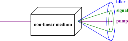
Bell’s theorem motivated to look for different sources of entangled states of particles/photons. In the early days, some of the methods to realize entangled states were spin zero molecules (as given by Bohm [3]), radiative atomic cascade of calcium to create polarization entangled bi-photon states [51, 52, 53] and non-linear optical processes. In recent years, a second order non-linear process known as spontaneous parametric down conversion (SPDC) has become a widely used method to create correlated photon pairs. In the SPDC process, a higher energy photon interacts with the non-linear medium and emits two lower energy photons, historically known as signal and idler (see figure 1). The SPDC process was first theoretically predicted by Louisell et al in 1961 [54] who
modeled it as two oscillators coupled via a time-dependent
reactance. Later, Giallorenzi et al [55] explained SPDC as the scattering process in which a pump photon is transformed into a photon-pair because of the non-linear polarization. It’s first experimental observation was studied by Harris et al in 1967 [56], later followed by many others. Burnham et al in 1970 experimentally confirmed simultaneous emission of signal and idler photons via coincidence detection [57]. The coincidence-detection study paved the road for use of SPDC photon pairs for fundamental study [58] as well as the application based explorations.
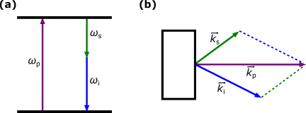
Boyd et al. [59] explains SPDC as a result from the second-order nonlinear polarization in noncentrosymmetric crystals. Assuming the absence of resonant atomic excitation and pump field strengths much smaller than the atomic field strength, this process will follow the laws of energy and momentum conservation in lossless media, figure 2 shows this schematically. Because of energy conservation, the total energy of the generated photons equals the energy of the pump photon. Therefore
| (2) |
with as the angular frequency of the pump, signal and idler photons, respectively. Equally, the momentum conservation laws are fulfilled with,
| (3) |
where , , and are the wavevectors of the pump, signal, and idler, respectively. As can be seen in the figure 2(b), to fulfill the momentum conservation, the transversal components of the momentum vectors are anti-correlated between the signal and idler photons. Both photons originate from the same positions in the crystal, leading to a direct correlation in the transversal position. Furthermore the generated photons show correlation in various degrees of freedom such as polarization [60, 61, 62, 63], orbital angular momentum (OAM) [64, 65, 32], energy-time [23, 22, 24, 21] and transverse position and momentum [66, 12, 67]
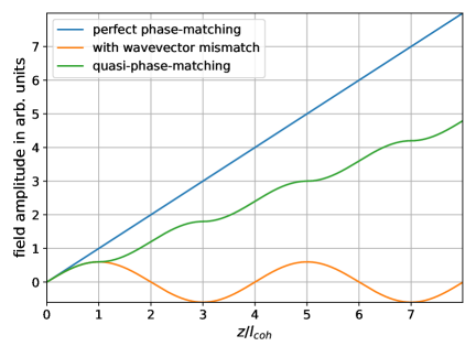
In order to achieve efficient SPDC, it is additionally necessary for the longitudinal momentum mismatch
| (4) |
with as the longitudinal component of the wavevector set to zero. This is called the phase-matching. As visualized in figure 3 there will be a linear dependence of the propagation length with the field amplitude of the generated SPDC signal, if the condition is fulfilled (perfect phase-matching). In case of , the field amplitude will vary periodically depending on the propagation length as a consequence of the generated light waves destructively interfering. The phase-matching is dependent on a multitude of parameters, e.g the involved wavelengths, the crystals internal structure, the temperature and more. Therefore the possible wavelength combinations for perfect phase-matching are limited in number. In the year 1962 Armstrong et al. [68] proposed to periodically modulate the sign of the second-order nonlinear coefficient of the material to shift the phase of the generated light waves. This method is called quasi-phase matching and is a versatile tool for increasing the possible spectral combinations of SPDC. As a consequence, the phase-matching condition for quasi phase-matching case changes to:
| (5) |
with as the period of the alternating second-order nonlinear coefficient.
I.3 Discrete variable entanglement
In the case of polarization, when phase matching condition is such that generated photons has the same polarization as the pump photon then it is known as the Type-0 phase matching. When generated photons has orthogonal polarization to that of pump photon then it is known as Type-1 phase matching and when the generated photons has orthogonal polarization with respect to each other then it is known as the Type-2 phase matching. The polarization correlation between the signal and idler have been extensively studied for fundamental tests as well as the quantum communication and information applications. The study of polarization correlation really exploded when Aspect et al. showed strong violation of Bell’s inequality for the first time in 1981 [51]. In their experiment, they studied the linear polarization correlation of the photons emitted in the radiative atomic cascade of calcium. This remarkable study ruled out the whole class of realistic local theories and became a foundational stone for many non-classical tests and applications. For such a worthy contribution, Alain Aspect altogether with Anton Zeilinger and John Clauser were awarded the Nobel prize in 2022.
However, the atomic cascade source is difficult to handle and has low brightness. To overcome this issue, Kwiat et al. used SPDC source consisting of BBO (beta barium borate) with type-2 phase matching [62]. With improved visibility of 97% they demonstrated violation of Bell’s inequality. They also mentioned a method to convert one Bell state into another (Eq.6) using unitary transformations.
| (6) | ||||
Generation of Bell states played crucial role demonstrating many quantum mechanical phenomenons like quantum teleportation[8], super-dense coding[69], entanglement based quantum communication[70], quantum metrology[49, 50], no-cloning theorem[71], etc.
In addition to linear polarization, light also possess circular polarization. Circularly polarized photon-states are the eigenstates of the spin angular momentum (SAM) operator with eigen values . This was first demonstrated experimentally by Beth in 1936[72]. Photons with linear polarization are associated with zero SAM. Unlike SAM, OAM of light is consequence of the helical wavefront and azimuthally varying phase [73]. OAM carrying beam has a phase singularity at the center of the beam and flow of energy spirals around the propagation axis hence it is famously known as the optical vortex (OV). Optical vortices carry OAM per photon, where is the order of orbital angular momentum. Spin angular momentum spans two-dimensional space, whereas OAM spans infinite-dimensional space ranging from to .
Along with the energy and momentum, conservation of orbital angular momentum is maintained as well in the SPDC process. Making use of this fact, Mair et al. [65] for the
first time showed entanglement generation of photons in the OAM degree of freedom. This work encouraged various other groups to explore the properties
of OAM in the quantum domain [74] for information transfer and processing [75]. Just as polarization state of photons represents a qubit, polarization state of photons represents qubit, OAM states of light have also been used to represent higher dimensional bit know as qudit. Orbital angular momentum states of light provide infinitely many orthogonal basis states that can be used to encode quantum information and may improve security [76, 77, 78]. Controlled generation of OAM entangled state is studied for secure quantum communication and information processing [79, 80, 81, 82, 83].
I.4 Continuous variable entanglement
Photons produced in the SPDC process are also correlated/entangled in continuous variables such as quadrature phase-amplitude[26, 27, 28], position-momentum entanglement[12, 13, 14, 15, 16, 17]. In recent years, the field of continuous variable entanglement study [12] has been explored. In [84], Reid and Drudmund derived EPR criterion to show how it could be utilized with position-like and momentum-like quadrature observables of squeezed states to show inseparability/entanglement. Shortly after that, [85, 86, 36] derived sufficient and necessary conditions for the continuous variable entanglement. Transverse correlations of the photons produced in the SPDC process have been studied both theoretically as well as experimentally [66, 87, 88, 89, 90].
Transverse position and momentum are the spatial variables of the signal and idler which follow EPR criterion. Howell et al. [12] were the first to report strong position-momentum entanglement in the photon pairs generated in the SPDC process. Using coincidence detection in the near and far fields, they measured position-momentum variance product of 0.01, which is direct indication of violation of the bounds for the EPR and separability criteria. The spatial entanglement is continuous variable entanglement and has gained attention in recent years, and found applications in the field of quantum imaging[39, 40, 41, 42, 43], quantum metrology [49, 50] and quantum communication[15, 91, 92, 37]. As discussed in the section II, conditional uncertainty/correlation length of the position and momentum of the two photons depends on several pump and non-linear crystal parameters. The momentum correlation length depends on the beam waist and the spatial coherence of the pump, whereas, the position correlation length depends on the crystal length and the wavelength of the pump beam. Several authors have shown effect of spatial coherence on degree of spatial entanglement [93, 16] whereas few have investigated the effect of different spatial profiles of pump beam on entanglement[17, 94, 95]. Such study have been found useful for tuning the spatial entanglement, for comparing position-momentum correlation length of the SPDC photons created using coherent laser and the incoherent LED, shaping the angular spectrum of the SPDC photons etc. Several other studies delve into propagation dynamics of the spatial entanglement [96, 97].
II Theoretical Background
As described in references [98, 89, 99], the quantum state of the biphotons generated in the SPDC process at the crystal face (z=0) in wave number space reads as,
| (7) |
where, is known as the mode function. and are the wave vectors of the signal and idler photons and are the corresponding creation operators. Under the condition of collinear phase matching condition where pump, signal and idler travels in the same direction, is given as,
| (8) | ||||
where N is the normalization factor, and is the transverse profile of the pump beam at the crystal plane. is the phase mismatch in the -direction. The sinc function describes the efficiency of the down conversion with varying phase mismatch. When phase mismatch is zero, i.e. , sinc function is maximized (). Value of sinc function decreases as the phase mismatch increases which in turn reduces the efficiency of the down conversion. represents the phase evolution of the signal and idler photons propagating in the -direction. represents the phase shift that arises from the phase mismatch within the non-linear crystal.
For the collinear phase matching condition, the sinc function in equation (8) can be approximated to a Gaussian with adjustment parameter (see equation (10)), also if we consider coherent Gaussian shaped pump beam ( is assumed Gaussian shaped) then the momentum space wave function of the bi-photons at the crystal plane takes the form as, [30, 99],
| (9) | |||
where, are the standard deviations of the two Gaussians and are related to transverse momentum and position correlation widths. represents the position correlation width of the bi-photons, and it is defined as below, where L is the crystal length,and is the wavelength of the pump beam.
| (10) |
and the momentum correlation length of the biphotons is inverse of the pump beam waist (),
| (11) |
By Fourier transforming equation (9), one can write biphoton wave function in position space as,
| (12) | |||
When the beam waist is much greater than the bi-photon position correlation width, i.e., . In this condition, from equations (9) and (12), one can see signal and idler exhibit position correlation and momentum anti-correlation. The effect of the various pump beam parameters on these correlations is discussed in detail in section V.
III Techniques to measure spatial entanglement
In general, position-momentum entanglement can be measured with various techniques using different resources and assumptions on the quantum system. These techniques can be categorized as entanglement estimation, entanglement certification, and entanglement quantification [100]. Entanglement estimation employs the most assumptions on the quantum systems and does not need to measure intensity or correlations in any plane. It follows the entanglement certification, which is enough to measure the intensity profile in the far field plane but assumes the purity of the quantum system. Finally, entanglement quantification is the most complete measurement since it measures the correlations in both planes: the far field and the near field. This type of measurement also has more developed techniques and experimental realizations because of its completeness. It includes methods such as direct detection of position-momentum of the signal and idler with slits, intensity correlation using EMCCD camera and 2D detector array and the measurement of cross-spectral density function of the interference at near- and far-field. Here, we review some of the most relevant techniques in the paraxial regime, starting from entanglement estimation, continuing with entanglement certification, and finishing with entanglement quantification.
III.1 Number of spatial modes
The number of spatial modes () can be estimated from the source parameters and the pump beam waist by [101, 44, 102, 103] as follows,
| (13) |
where () is the refractive index of the medium for the idler (signal) photon, is the crystal length, and () is the wavelength of the idler (signal) photon. We can note that the number of spatial modes does not depend on any optical system assumption in any plane. Thus, the number of spatial modes delivers a rough estimation of the spatial biphoton properties that can be found in either plane.
III.2 Schmidt number
Entanglement can be certified by mode decomposition using the Schmidt number, . Let us recall the biphoton joint amplitude of signal and idler modes . This function can be decomposed as [104]
| (14) |
where the Schmidt number are eigenvectors of the reduced density matrix for the signal, , and for the idler photon, , and are the eigenvalues. With these parameters, the Schmidt number decomposition delivers information about the two-photon state. The modes and show how the signal-idler pair are spatially correlated, while the value of represents the degree of entanglement of the system. A convenient form for the Schmidt number is , where corresponds to a separable state, and corresponds to an entangled state. The Schmidt number can be experimentally obtained by measuring the intensity profiles in the near and far fields [105, 106]. However, in this certification measurement of spatial entanglement, purity is assumed on the quantum systems. Alternatively, the Schmidt number can also be measured using coherence, as shown in Ref. [107].
III.3 Direct detection in the near and far field
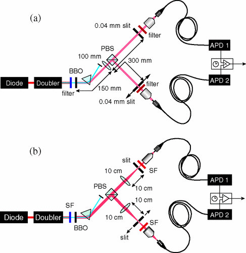
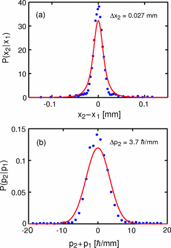
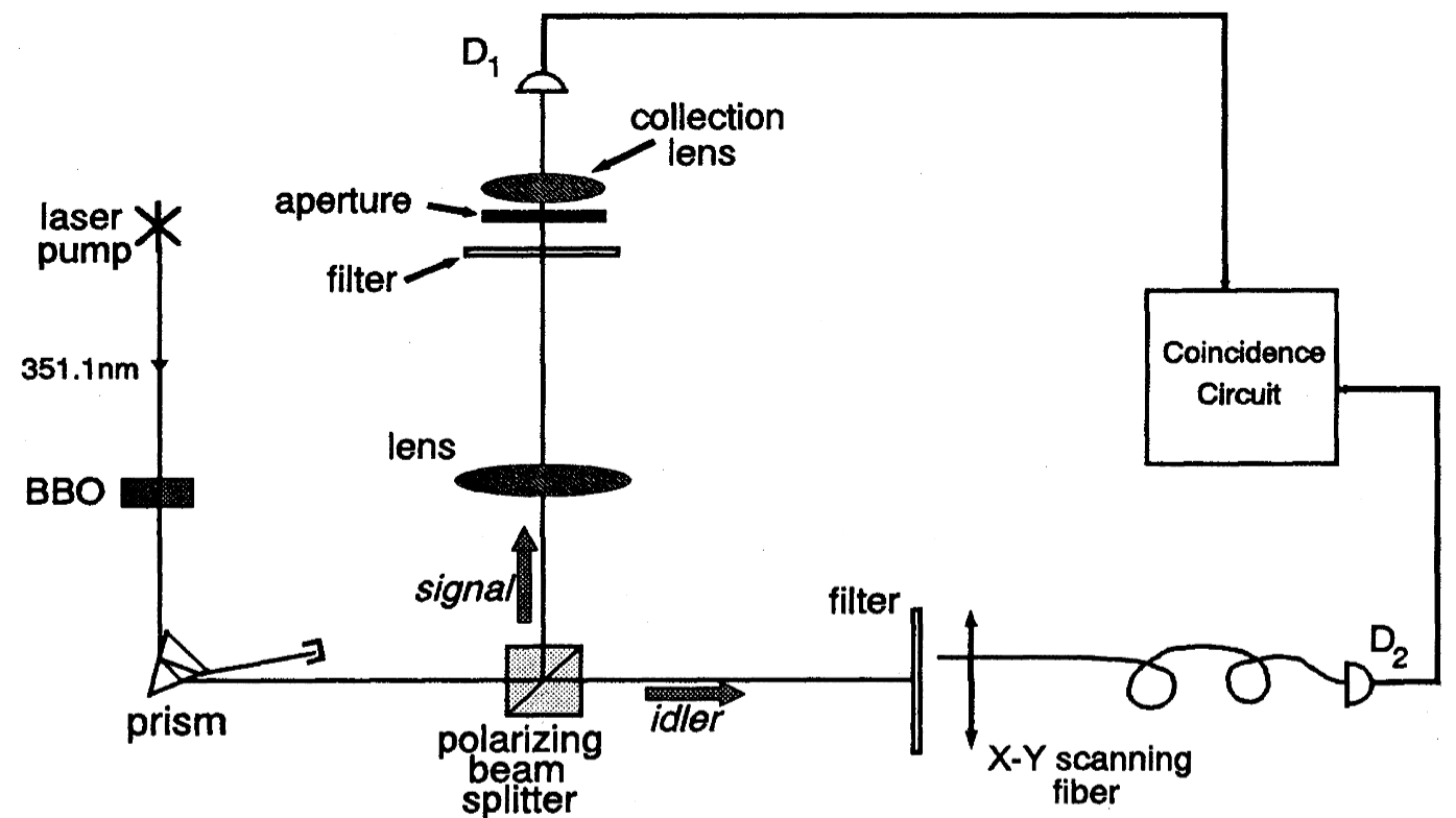
From this section onward, we discuss methods that are based on correlation measurements at near- and far-field. In reference [12], authors have reported experimental realization of the EPR paradox using position-momentum entangled photons. In the experimental setup, 2 mm long type-2 BBO crystal is pumped with the 390 nm laser which creates SPDC photon pairs. A prism is used to separate the down converted photons from the pump beam. Orthogonally polarized signal and idler are separated using polarizing beam splitter (PBS). Two slits of width 40 m are placed into the two output arms of the PBS. To measure position and momentum correlation widths, lenses in near-field and far-field configurations are placed. For the position correlation, the crystal plane is imaged onto a slit using a 100 mm lens. The lens is kept such that it’s distance from crystal to lens is 150 mm and from lens to slit is 300 mm, as shown in figure 4(a). To measure transverse momentum correlation, two 100 mm lens are kept in two arms of the PBS such that, their distance from slit is 100 mm. This configuration does a Fourier transformation of the transverse position onto the slit, as shown in figure 4(b). These lenses map transverse momenta to transverse positions such that the transverse momentum of the signal/idler, , focuses to the point , where is the transverse wavevector and . In both cases, one of the slits (slit-1) is fixed at peak single counts while the other slit (slit-2) is free to move in -axis. Behind each slit, there is a nm band-pass filter followed by the objective coupled to the multimode fibers which are connected to coincidence counter. Coincidence count rate is recorded as function displacement of the slit-2. This gives distribution of coincidence counts against the displacement of the slit-2 for position and momentum. By normalizing coincidence distribution, conditional probability for position and for momentum are obtained, where 1 and 2 represents signal and idler, as shown in figures 5(a) and (b). These probability distributions are then used to calculate uncertainty/standard deviation in position and momentum of the second photon when position/momentum of the first photon is fixed using slit-1. The experimentally obtained value of is 0.027 mm and the value of is mm-1. The product of variance for position and momentum violates separability bound by 2 orders of magnitude as,
| (15) |
Theoretically, for given crystal thickness, pump beam wavelength and waist variance yields which is lesser than the experimental value. Thereports explanation for this discrepancy is perhaps the coincidences from optical components. Additionally, it should be noted that, because of the broader slit width (40 ) conditional probability distribution is broader than the one it is associated to the SPDC process by itself.
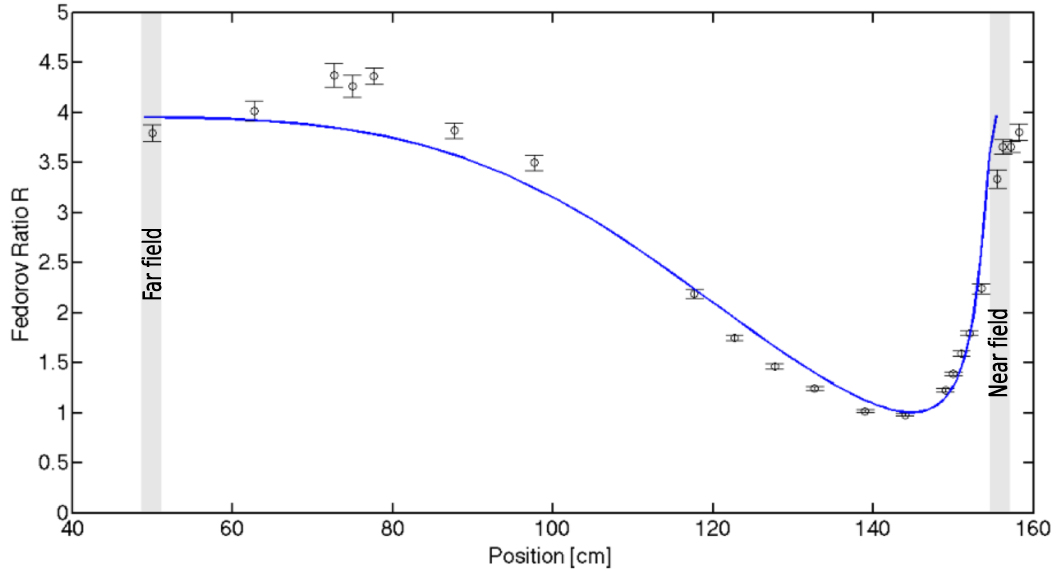
Noteworthy to mention an additional technique that quantifies the spatial entanglement by measuring intensities and correlations in both planes: the Fedorov ratio [108, 109, 107]. In it, the intensity profiles are divided by the conditional probability of the biphotons in far-field and near-field planes. When the Fedorov ratio equals 1, no entanglement is present in the system. However, this measurement technique fails when measured between the near field and the far field, as the value of 1 does not represent a system without entanglement. The reason for this is that the spatial entanglement is transferred from the amplitude to phase while it moves from the far field to the near field, see figure 6. More details in Refs. [110, 108].
III.4 Correlation imaging using a camera
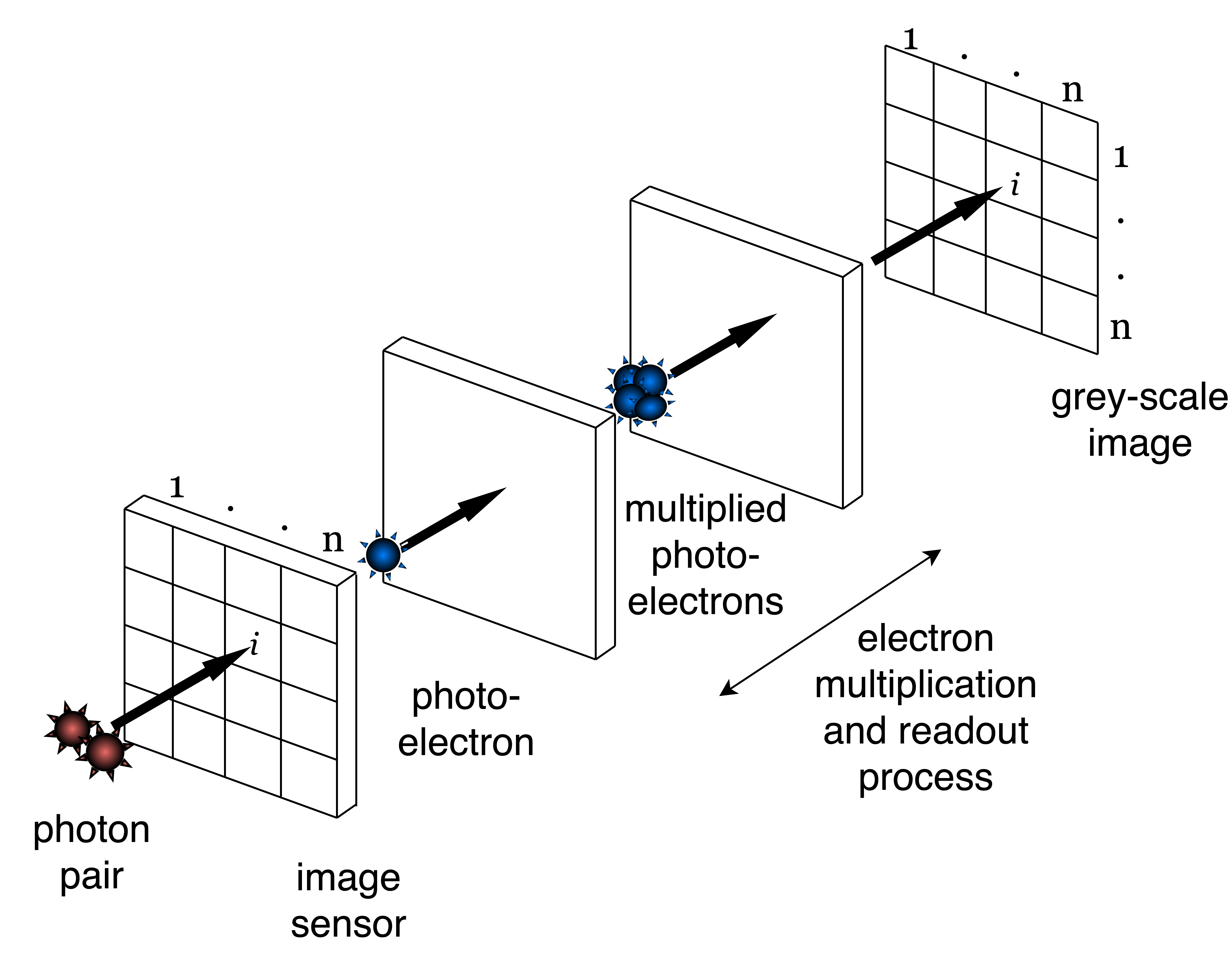
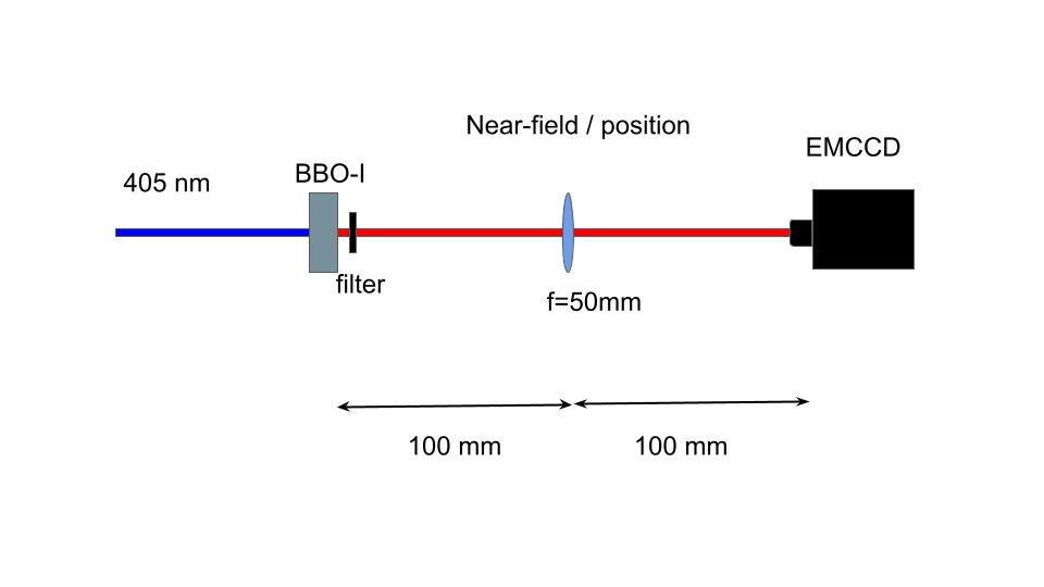
With the advancement in detection technology, a weak signal can be detected and registered with quantum efficiency 90% using an electron-multiplying CCD (EMCCD) camera. The general scheme to extract correlation using EMCCD camera uses the sub-Poissonian statistics of photon pairs and is described in details in [111]. Several other authors have also used EMCCD cameras and 2D detection arrays for measuring spatial entanglement [30, 17, 112, 113, 114, 115, 111, 13, 40]. In simple form, the schematic of this technique is depicted in figures 8 and 9. A non-linear crystal is pumped by a continuous wave laser of wavelength 405 nm. A band-pass filter is kept after a non-linear crystal to block pump beam and let pass the generated SPDC signal of wavelength 810 nm. For near-field/position correlations, a lens of focal length 50 mm is kept at 100 mm from the crystal, and an EMCCD camera is kept at 100 mm from the lens. This configuration allow to image crystal plane onto the EMCCD camera without any magnification (M=1). For far-field/momentum correlations,the 50 mm lens is replaced by a lens of focal length of 100 mm keeping the distances between the components, crystal, lens and camera. This configuration performs Fourier transformation of the crystal plane onto an EMCCD camera. The far-field imaging maps the transverse momentum of the photons onto position coordinates (pixels) of the EMCCD. Considering optimization of signal to noise ratio [116], exposure time of an EMCCD and pump power is adjusted. Then multiple frames (millions) are captured which has only intensity information of all the SPDC photon pairs falling onto the camera.
As depicted in figure 7, one of the photons from the photon pair hits the EMCCD camera sensor at pixel i (while the other lands at pixel j) which is then converted into photoelectrons with quantum efficiency . These photoelectrons are then multiplied in amplification process so that the weakest signal becomes readable. Then, amplified electrons are converted into grey-scale values corresponding to pixel i(j).
To measure the spatial correlations, joint probability distribution (JPD) is calculated in near and far-field configuration. The JPD represents probability of detecting one of the photon from pair at pixel i and other at pixel j and it is defined as, [93, 111, 39, 17, 117]
| (16) |
where, N is the totatl number of frames, the first term is the intensity correlation of the pixel i with the rest of the pixels in the same frame (l). This term gives the coincidences due to the photon pairs as well as coincidences with the noise or with the photons from other photon pairs. Whereas, the second term gives the intensity correlation between pixel i of the frame l with the rest pixel j of the next frame l+1 (). Since SPDC photons are created simultaneously and reach the image sensor simultaneously for the given exposure time, the second term will only have accidental coincidences. By subtracting second term from the first term, true coincidences due to SPDC photon-pairs are obtained.

To measure correlations of all photon pairs in a frame at once, one can sum the frame along rows or columns as shown in figure 10(a). Summing along rows adds all grey-scale values in turns associated intensity along -axis. This summation transforms the matrix into column matrix which has the information of intensity correlation in -axis. So, correlations in y-axis can be obtained by summing frames along rows while correlations in -axis are obtained by summing frames along columns. For the same frame (l), multiplying transpose of the column matrix with the column matrix as shown in figure 10(b) gives the pixel to pixel intensity correlation within frame l, this represents the first term of the equation (16). To get the second term in equation (16), column matrix obtained from frame l is multiplied with the transpose of column matrix of frame . Subtracting these two multiplied matrices gives the information of true coincidences. Diagonal elements of subtracted matrix is associated with the intensity correlation of a pixel with itself. This tells probability of detecting signal and idler at the same pixel. First sub-diagonal elements show the intensity correlation between two adjacent pixels, which gives the probability of detecting signal and idler at two adjacent pixels and so forth. For position correlation, taking diagonal summation over correlation matrix gives double Gaussian distribution which is the joint detection probability of signal and idler for various distance between them. Similarly, when summation is taken anti-diagonally, double Gaussian distribution gives the joint detection probability of momentum of signal and idler for different mapped as position on the camera.
The standard deviation of this Gaussian distribution gives the conditional uncertainty in the measurement of position and momentum at the EMCCD sensor plane. In order to get the values of conditional uncertainty at the crystal plane, the transformation equations described below are used.
| (17) |
where is the position correlation length at the EMCCD plane measured using near-field imaging with magnification ( M=1 for no magnification), is the momentum correlation width mapped in position coordinates of the EMCCD at the far-field, is the wave-number of the SPDC photons, and is the focal length of the lens used for the Fourier transform of the crystal’s exit plane onto the EMCCD.
In quantum imaging, JPD is a quantity of particular interest. JPD is achieved through statistical averaging roughly over to intensity images. Given the fact that CCD-based detectors provide frame rates of the order of 100 frame per second, total acquisition time to achieve JPD can vary from several hours to over a day. Such long acquisition times hinders the adaptation of quantum imaging schemes for real world applications.
In recent years, single-photon avalanche diode (SPAD) cameras have been produced and are now commercially available. These cameras are based on CMOS technology. The progress in this field has empowered the production of compact arrays [118, 115]. So far, SPAD arrays have demonstrated their capabilities in LiDAR(Light detection and ranging) [119, 120, 121], fluorescence lifetime imaging [122, 123, 124], imaging through strongly scattering media [125], non-line of sight imaging [126], time-resolved correlation measurements [127, 128].
In the article [13], the authors demonstrate spatial entanglement using an SPAD. Using an SPAD array, they achieved spatial entanglement by violating the EPR criterion with a confidence level of 227 sigmas for acquisition time of just 140 seconds. For better signal-to-noise ratio, large number of frames of order of to are acquired. Typically, EMCCD takes several hours to over a day to acquire to images. Whereas, with the SPAD array, acquisition time drastically shortened indicating its capabilities in real world applications. Moreover, they confirmed the high-dimensional entanglement up to 48 dimensions in just . Authors also emphasis on the entanglement certification using SPAD technique is significantly faster () than the usual projective measurement techniques [129, 130, 131]. This indicates the potential use of SPAD array in the field of high-dimensional systems.
III.5 Using cross-spectral density function
Coincidence-based EPR correlation measurement techniques face challenges such as excessive signal loss, the need for multiple measurements, or stringent alignment requirements, all of which negatively impact measurement quality.
In the method, well discussed in the reference [132], the EPR correlations are measured without coincidence detection. This technique works for two-photon states that are pure, irrespective of whether the state is entangled or separable.
It is well known that, for continuous variables of two-photons, properties such as two-photon angular Schmidt spectrum [133, 134, 135], two-photon spatial Schmidt number [136], and momentum correlations [137] can be measured by doing intensity measurements on only one of the photons. These measurement techniques based on intensity detection provide much better accuracy than those based on coincidence detection.
In transverse momentum basis, a pure state of two photons can be written as,
| (18) |
where, and are the transverse momenta of the signal and idler photon respectively. is the two-photon state vector, and is the two-photon transverse-momentum wavefunction. The conditional momentum probability distribution of the signal photon when the idler photon is detected with transverse momentum is given by,
| (19) |
The momentum cross-spectral density function of the signal photon can be calculated as , where and are the positive- and negative-frequency parts of the electric field operator, respectively. For ,
| (20) |
If the two-photon wavefunction satisfies the following condition
| (21) |
| (22) |
Equation (22) states that, as long as a two-photon state is pure, and satisfies equation (21), the momentum cross-spectral density function of the signal photon remains proportional to its conditional momentum probability distribution function. Therefore, the standard deviations of and are equal and by measuring the standard deviation of , one can obtain the standard deviation of . For x-position, standard deviation is represented by .
One can write equation (18) in position bases to show that if the two-photon position wavefunction satisfies the condition,
| (23) |
where and are the transverse position of the signal and idler photons, then the position cross-spectral density function of the signal photon is proportional to its conditional position probability distribution function , that is,
| (24) |
Thus by measuring standard deviation of , one can obtain the standard deviation of . For -position, standard deviation is represented by .
A non-separable state violates the inequality shown in equation (25) and this implies that two photons are entangled having EPR correlations in position-momentum variables.
| (25) |
III.5.1 Method and results
In the experiment; 2 mm thick type-1 collinear phase matched BBO crystal is pumped using continuous wavelength laser of wavelength 405 nm and beam waist =388 m. The interferometer shown in figure 12(a) is used for measuring position cross-spectral density function of the signal photon at the crystal plane and use a imaging system with =10 cm and =40 cm to image the crystal onto the EMCCD camera plane with a magnification of M=4. Position coordinates at the crystal plane are shown as and that at the EMCCD plane are shown as (). These sets of coordinates are related as and . The interferometer uses the wavefront inversion technique to measure cross-spectral density function [134, 138]. The intensity of the output interferogram at the EMCCD plane is given by,
| (26) | ||||
here, and are the scaling factors, and and are the intensities at the EMCCD plane coming through the two arms of the interferometer and the is the phase difference between two interferometric arms. For two different phases, one can show that the difference intensity is proportional to the position cross-spectral density, that is, . Figures 12(b), (c) show the interferogram at and and figure 12(d) shows the difference intensity . From equation (17), one dimensional conditional position probability distribution function is obtained by averaging over the -direction and plotting it in figure 12(e). By adjusting the magnification factor , the experimental value of was obtained as 6.56 m, which is close to the theoretical value of 7.65 m.
To measure the momentum conditional probability distribution function, a lens configuration with =5 cm, = 10 cm and =30 cm is used for imaging the Fourier plane of the crystal onto the EMCCD camera. The effective focal length of this configuration is =15 cm. The transverse momentum at the crystal plane is related to the transverse momentum at the EMCCD camera plane () as, , where . Same as discussed for the position, the difference intensity is obtained as, . Again using equation (17), and by adjusting for momentum coordinates at crystal and EMCCD plane, experimentally obtained value of to be m which lies very close to the theoretical prediction m.
For the obtained standard deviation for position and momentum, the value for equation (25) is , which is much smaller than and thus implies strong EPR correlations between two entangled photons. To measure the accuracy of the experiment the authors defined the quantity . Smaller values for imply a better experimental accuracy for the EPR correlation measurements. They obtained a value which is smaller than the value reported by several other authors [12, 31, 30, 139, 14]. There is another quantity defined to quantify the EPR-correlations named degree of violation and it is defined as, . The degree of violation does not quantify the accuracy but gives an estimate of the degree with which the Heisenberg bound of 0.5 is violated. For their experiment, , whereas the degree of violations reported earlier [12, 31, 30, 139, 14] has lower values.
IV Confidence level of EPR violation
A parameter known as confidence level is often associated with the EPR violation [13]. A high confidence level indicate that measured correlations in the experiment are strong and robust. That means, a high confidence level ensure that the generated high-dimensional source can be trusted to be used for quantum applications. Mathematically, the confidence level is defined as,
| (27) |
where is the propagation of uncertainty in the multiplication of two quantities and it is given as,
| (28) |
where and are the uncertainties in the measurements of and , respectively.
For the entanglement value, = , in the reference [13], the obtained confidence level is 277 . Such a high level of the confidence confirms that generated high-dimension entanglement has extremely strong correlations.
V Effect of spatial coherence on entanglement
To understand carefully how the spatial coherence of the pump beam influences the spatial correlation, the experiment by W. Zhang et al. [16] can be taken into sight. In the experimental setup shown in figure 13, in the blue-shaded part of the setup, they employ an LED to serve as a spatially incoherent light source, whereas in the red-shaded part, they employ a coherent laser followed by a spatial light modulator (SLM) that manipulates the transverse phase profile of the light. A nonlinear crystal is used to generate SPDC, and finally, a PBS is used to guide the correlated photon pairs into individual arms.
Using the direct detection method described in section III.3, the near- and far-field JPDs are measured for both LED and laser. The experimentally measured position-momentum JDPs for LED and laser can be seen graphically in the figure (14). The position of the signal and idler photons are highly correlated, and both show a sharp Gaussian peak for the case of pumping with the laser shown in figure 14(a) and for the case of the LED shown in figure 14(c). This shows that the position correlations are not affected by the spatial coherence of the pump beam, as it only depends on the crystal length and the pump wavelength as described in equation (10). The momentum anti-correlation shows a sharp Gaussian peak in figure 14(b) for the case of pumping with a spatially coherent beam from the laser. However, for pumping with an spatially incoherent beam from the LED the Gaussian distribution broadens significantly as it can be seen in figure 15(d). The distribution’s broadening width shows that the pump beam’s spatial coherence affects the momentum distribution. Using a Gaussian-Schell model for the partial spatially coherent beam [140] and a Gaussian approximation for the down-converted field [141, 142, 143], the momentum correlation width is given as follows:
| (29) |
where is the coherence length of the pump beam and is the beam waist. For perfectly coherent pump beam (), equation (29) returns to equation (11).
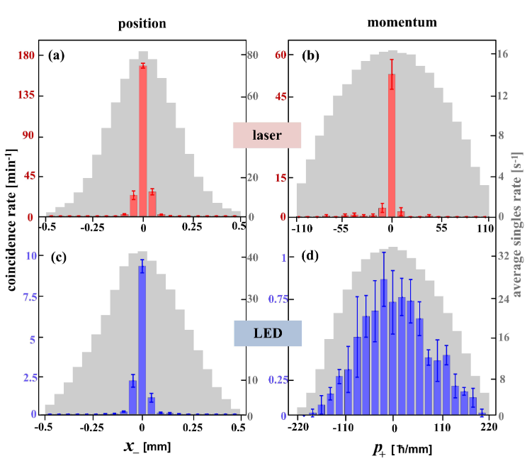
The resulting effect of the spatial coherence of the pump beam on the JPD is shown in figure 15. Figure 15(a) and (b) shows the position and momentum correlation for the case of pumping with a laser. Figure 15(c) and (d) shows the position and momentum correlation for the LED-pumping, respectively.
Furthermore, to verify the entanglement, measurement of the EPR criterion (see equation (1)) was carried out and resulted in the following factors:
| (30) |
which is well below 0.25 , indicating strong position-momentum entanglement when the laser is used as a pump beam, and
| (31) |
which is higher than 0.25 , indicating the absence of spatial entanglement.

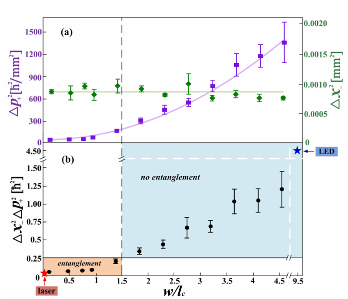
The behavior of momentum, position correlations, and entanglement for different spatial coherence of the pump beam can be seen in figure 16. Figure 16(a) shows that the position correlation remains intact for different whereas the momentum correlation keeps on losing strength. Figure 16(b) shows that the correlated pairs lose the spatial entanglement as the coherence in the pump beam decreases and makes a transition to classical correlations. The red star for using the laser as a pump shows strong entanglement in the correlated photon pairs, and the blue star for using the LED as a pump shows classical correlations.
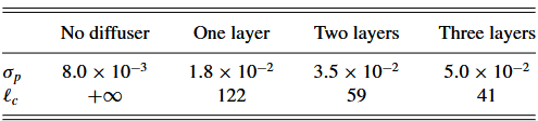
Another interesting work [142] on position-momentum correlations shows that while the position correlations remain intact, the momentum correlations weaken with the change in spatial coherence of the pump beam. Here, the coherence of the pump beam was disturbed using a series of plastic sleeves (diffuser). The setup shown in figure 17(a) consists of illuminating a BBO crystal with a partially coherent source. Such a source is created by successively adding rotating plastic sleeves that act as thin diffusers. The results of the experiment are presented in figure 17(c), which shows that regardless of the number of rotating diffusers, the position correlations remain the same.
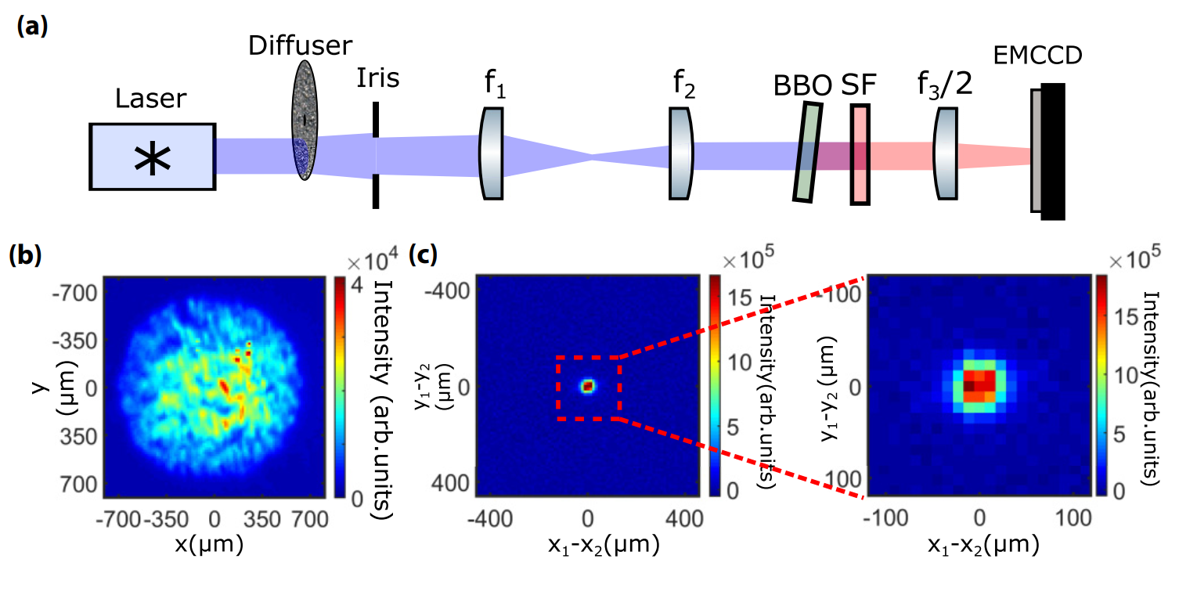
As shown in figure 18, the pump coherence is gradually reduced by introducing layers of plastic film, which gradually disturbs the coherence of the pump beam. With each additional layer, the pump beam became less coherent, worsening the momentum correlations.
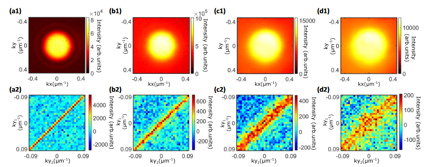
As the coherence decreases, the momentum correlations gradually weaken, and widens, which is illustrated in figure 19(a). This further states that as the coherence length of the pump beam decreases, the momentum correlations weaken, which stays consistent with predictions from the Gaussian-Schell model. Furthermore, a broader momentum distribution corresponds to a depletion in spatial entanglement. This shows a gradual degradation in the quality of momentum correlations, providing a controlled way to reduce entanglement rather than losing it abruptly, offering a tunable approach to control the degree of entanglement. The modification in the degree of spatial entanglement of the SPDC can be estimated using Schmidt number , which is defined as:
| (32) |
Figure 19(b) shows how the Schmidt number varies as a function of decreasing coherence length of the pump beam.
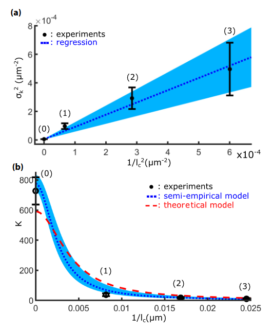
Figure20 presents the computed values of the correlation width as the coherence length decreases. The correlation width remains minimal when the pump beam has an infinite coherence length. However, the correlation peak width increases as the coherence length is reduced by introducing plastic sleeves layer by layer.
VI Engineering Joint Probability Distribution
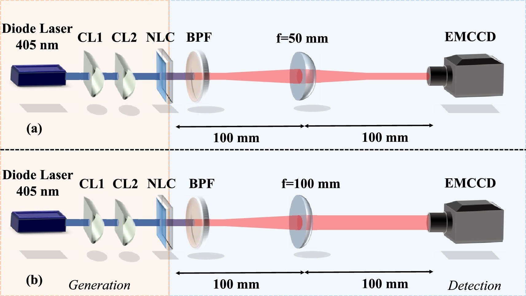
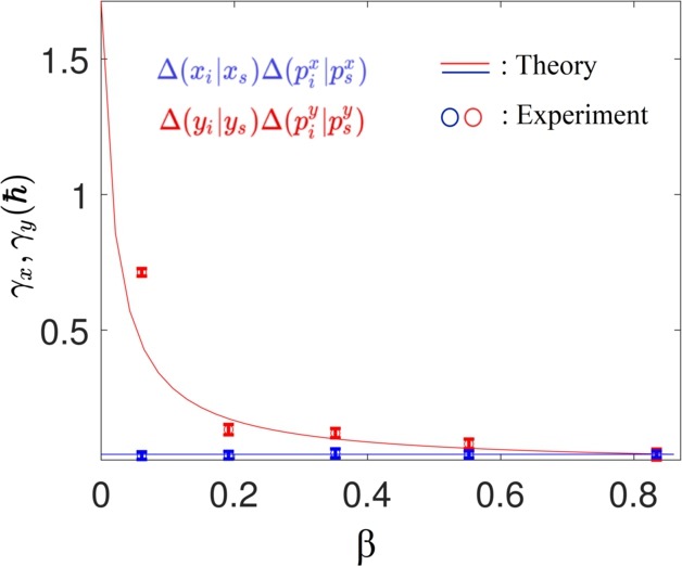
To tailor the shape of the JPD of the down-converted photons, one can directly act on the down-converted photons or one can modify the spatial shape of the pump to change the angular spectrum of the down-converted photons. Methods that act directly on the SPDC photon pairs include wave-front shaping [144, 145], quantum interferometry [146, 147], metasurfaces [148, 149], and rotating diffusers [150]. Whereas some methods achieve control over the spatial JPD through spatial shaping of the pump beam [151, 17, 94], real-time shaping of the down-converted photons by controlling the pump beam [152]. In this section, we only elaborate on the influence of the pump spatial profile on the JPD of the down-converted photons. In reference [17], the author modifies the shape of the Gaussian beam into an elliptical Gaussian pump beam using two cylindrical lenses, as illustrated in figure 22. An elliptical Gaussian beam has different beam waist sizes in the - and -directions. A different cylindrical lens with different focal lengths produces elliptical beams with a distinct beam waist ratio along to direction. To quantify the degree of ellipticity in the beam, parameter is defined as : where, and are the beam waists along and directions, respectively. Due to the distinct beam waist along - and -direction, the JPD of the momentum along - and -direction have a different value. The bi-photon state for -axis is given as (9), similarly for the -direction.
Theoretically, for coherence lengths much larger than the beam width, the momentum correlation length along and axes are given as,
| (33) | |||||
| (34) |
Since position correlation only on the wavelength of the pump beam (see equation (10)), position correlations do not change. To correlate the beam shape with the inequality value, parameters and are defined as,
| (35a) | |||||
| (35b) | |||||
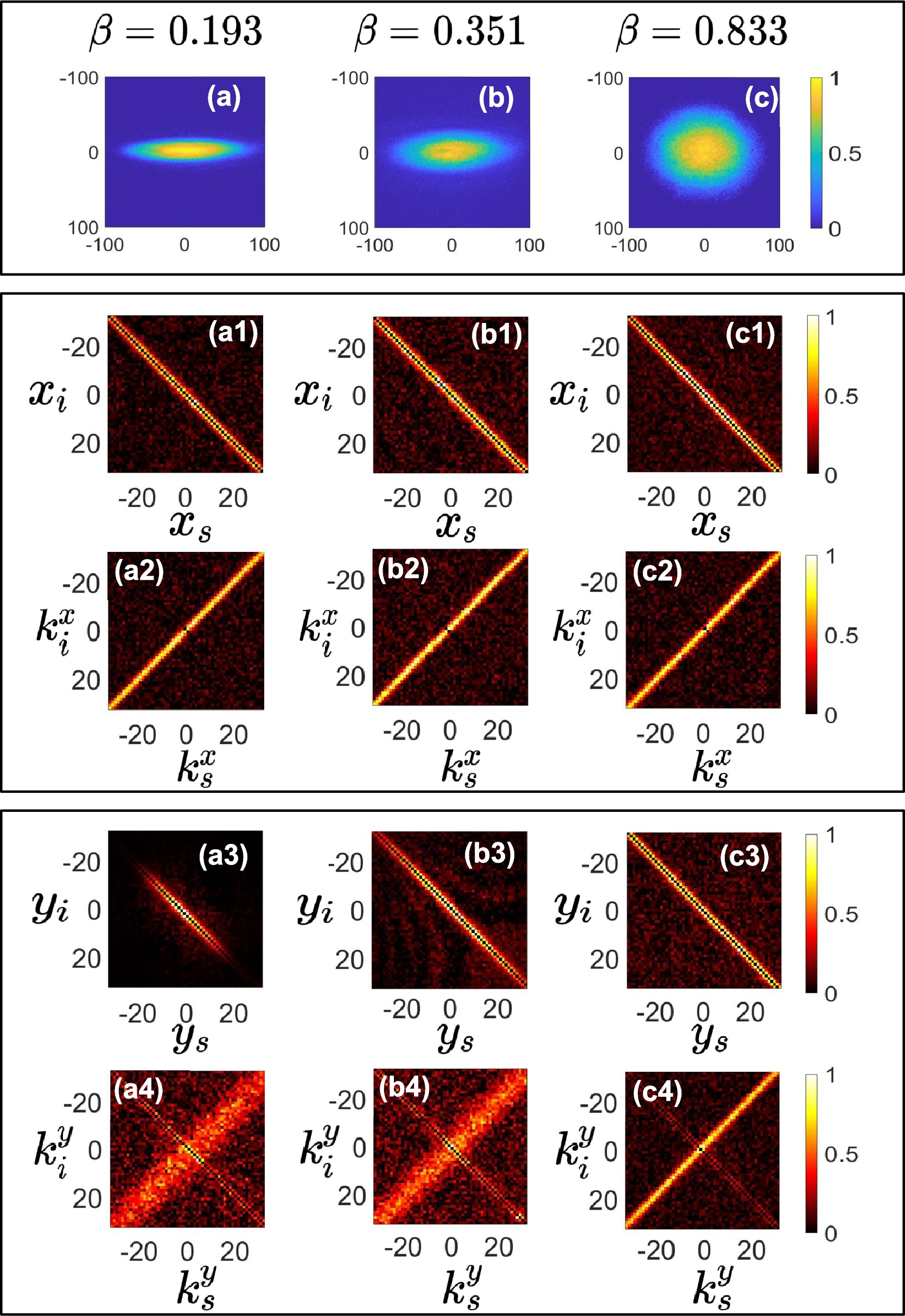
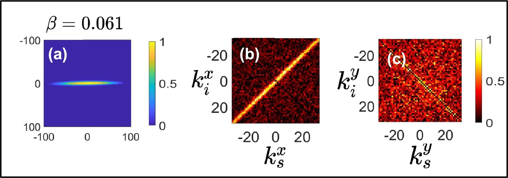
The experimental setup is shown in the figure 21. The JPD is estimated using method discussed in the section III.4. Figure 22 displays the JPD for various elliptical pump beam values. Figures 22(a-c) corresponds to elliptical pump beams with = 0.193, 0.351 and 0.833 respectively. The position JPD in - and -axis does not change (figure 23(a1-c1, a3-c3)) with the change in ellipticity. However, the momentum JPD in -axis remains constant (figure 23(a2,b2,c2)), whereas it changes in y-axis (figure 23(a4,b4,c4)). Plot 23 shows entanglement values along - and -axis. For the -axis, the entanglement remains constant because the beam waist does not change along the -axis. Where as entanglement along y-axis deteriorate as the beam waist along becomes narrower. If the pump beam exhibits a high ellipticity ( = 0.061), the momentum correlation along the -axis becomes weak enough to degrade entanglement along this axis. Simultaneously, the entanglement along the -axis remains unchanged. Creating strong entanglement in one direction while erasing the entanglement in other is a unique feature that can be useful for entanglement manipulation.
VI.0.1 Beam shaping
In another reference [94], a generalized study of spatial shaping of the pump has been reported. The spatial profile of the pump beam is modified using a spatial light modulator (SLM). The setup for the experiment is shown in the figure 26. A continuous wave laser illuminates the SLM that tailor its beam profile and impinges on a type-1 non-linear crystal using a imaging system. To get the angular spectrum of the generated SPDC photon-pairs, a lens with focal length is inserted between crystal and the EMCCD camera, where is the distance between camera and the non-linear crystal.
The pump beam with Bessel-Gaussian shape is given as,
| (36) |
where A is the constant, is the Bessel function of the first kind, is the beam waist of the Gaussian component and is the radial spatial frequency and represents the azimuthal angle. The angular spectrum i.e., the Fourier transform of the Bessel-Gaussian beam in equation (36) is given as,
| (37) | ||||
where, , and is the order modified Bessel function of the first kind. From this, the two-photon state generated using zeroth order Bessel-Gaussian pump beam is given as,
| (38) |
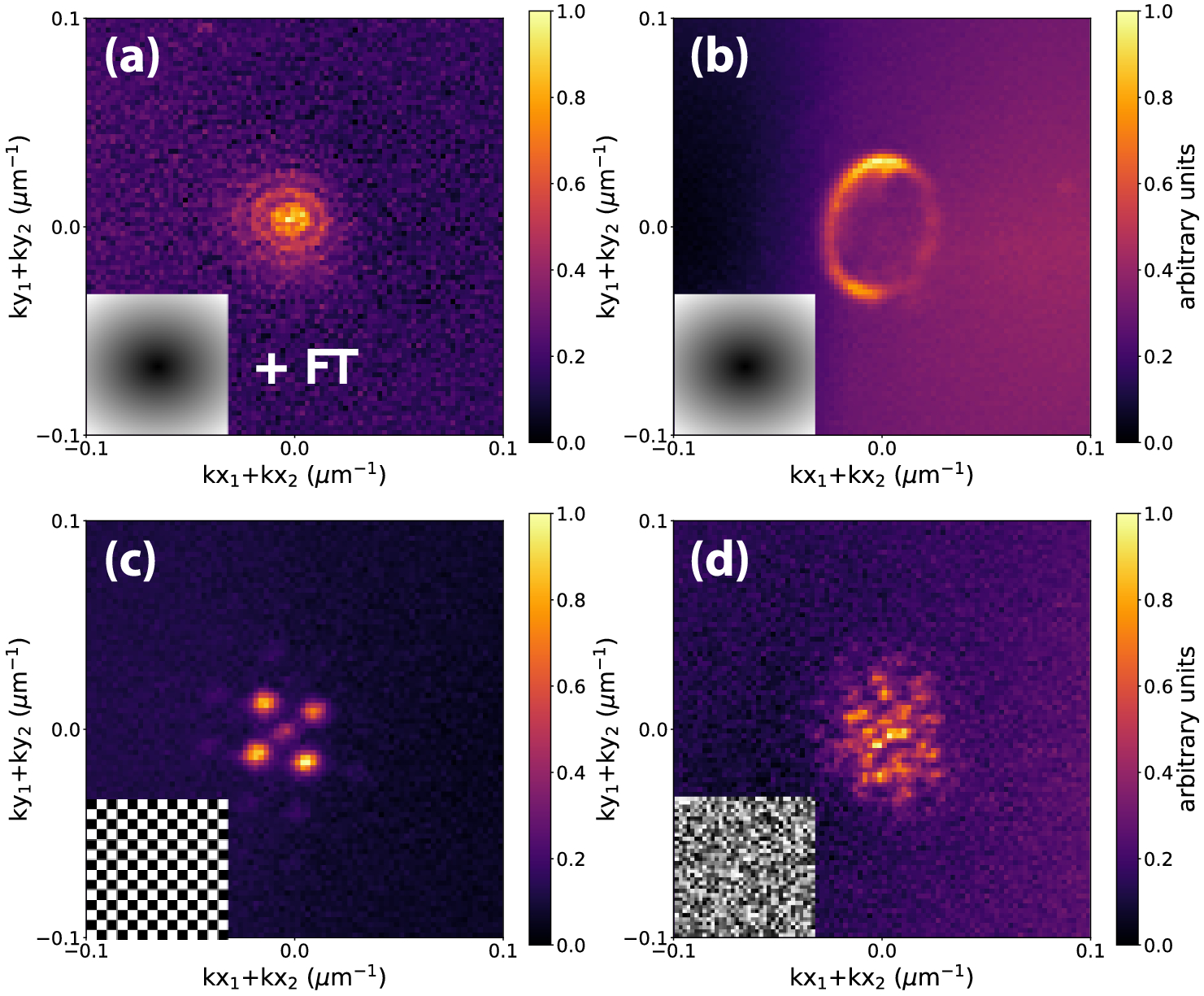
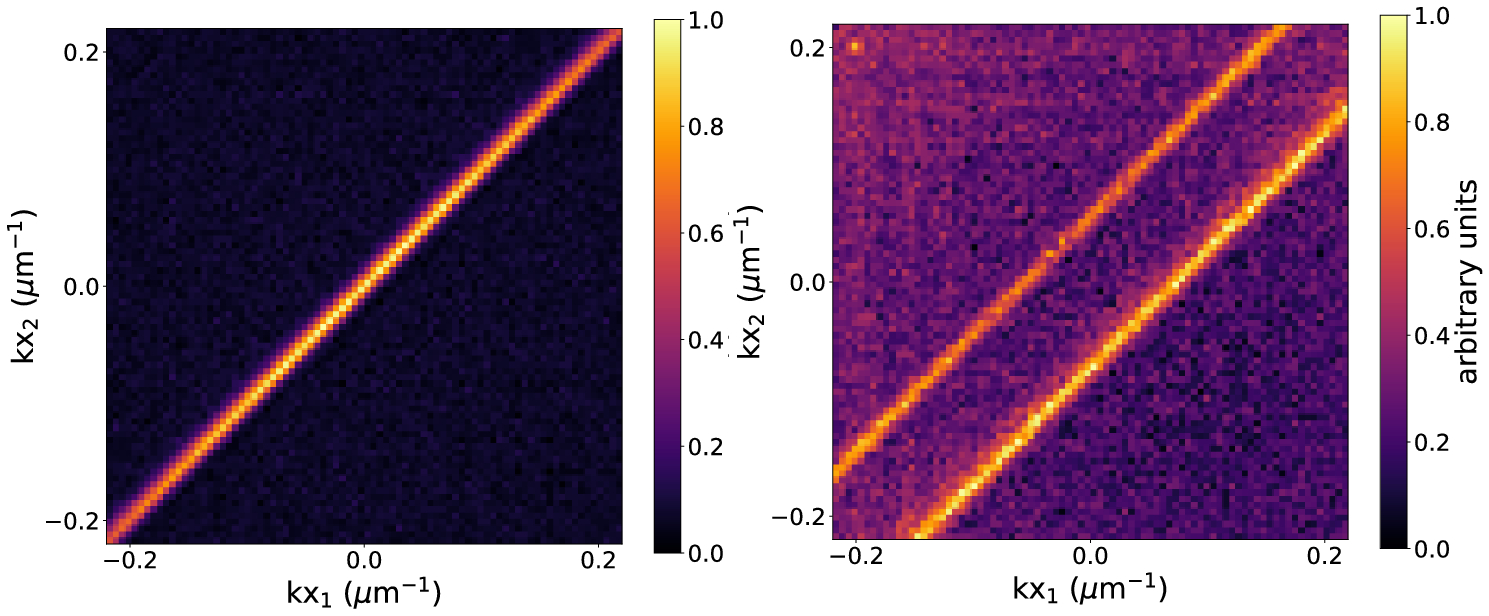
The JPD () is calculated using the method discussed in the section III.4. Figure 28 shows the anti-correlation in the momentum coordinate of the SPDC photons for Gaussian and Bessel-Gaussian pump beams. For a Bessel-Gaussian pump beam, the anti-correlation splits into two. This shows the possibility for correlation engineering. The observed autoconvolution of the down-converted photons has a ring shape for the Bessel-Gaussian pump beam, as seen in figure 27(b). The autoconvolution is defined as the projection of the JPD from the photon-pairs in the sum-coordinate basis { }, i.e., . Similarly, when the Fourier transform of the Bessel-Gaussian beam, (which is known as the perfect optical vortex [153]) is pumped to the crystal, then the autoconvolution of the down-converted photons has the Bessel-Gaussian shape, as shown in figure 27(a) . When the checker-board shape is displayed onto the SLM, the autoconvolution takes the shape shown in figure 27(c). Additionally, for the random pattern, it shapes likewise in figure 27(d).

VII Propagation of Spatial entanglement
Understanding the dynamics of the spatial entanglement becomes crucial, specially when used for the quantum communications. Study the dynamics of entanglement allows us to know how spatial entanglement evolves and changes as the entangled photons propagate through space or optical elements. Moreover, it helps in the optimization of quantum communication systems as
in building more efficient systems. Studying the propagation provides the insights necessary/useful to control and shape the spatial properties of the entangled photons. As discussed earlier and in section VIII, position-momentum entanglement has been used for several applications but it has been not been found suitable for applications dealing with long-distance propagation. This is because as the entangled photons propagate through space, the position-momentum entanglement decays dramatically fast [154, 143]. Additionally, in the presence of turbulence. On the other hand, as reported in the reference [97], angle-OAM entanglement initially decays with propagation but as the entangled photons travel further, the entanglement in angle-OAM bases is restored. They call this phenomenon as the propagation-induced revival of angle-OAM entanglement.
For the Gaussian pump beam with beam waist = at the crystal plane , the two-photon wavefunction in the position basis at the distance from the crystal is given as,
| (39) |
where A is the normalization constant, and are transverse position of signal and idler photons respectively at , and , , and . Moreover, is the same as in equation (10) at , i.e., the crystal plane and is a phase factor. At a distance of , the two photon probability distribution function = is given by,
| (40) |
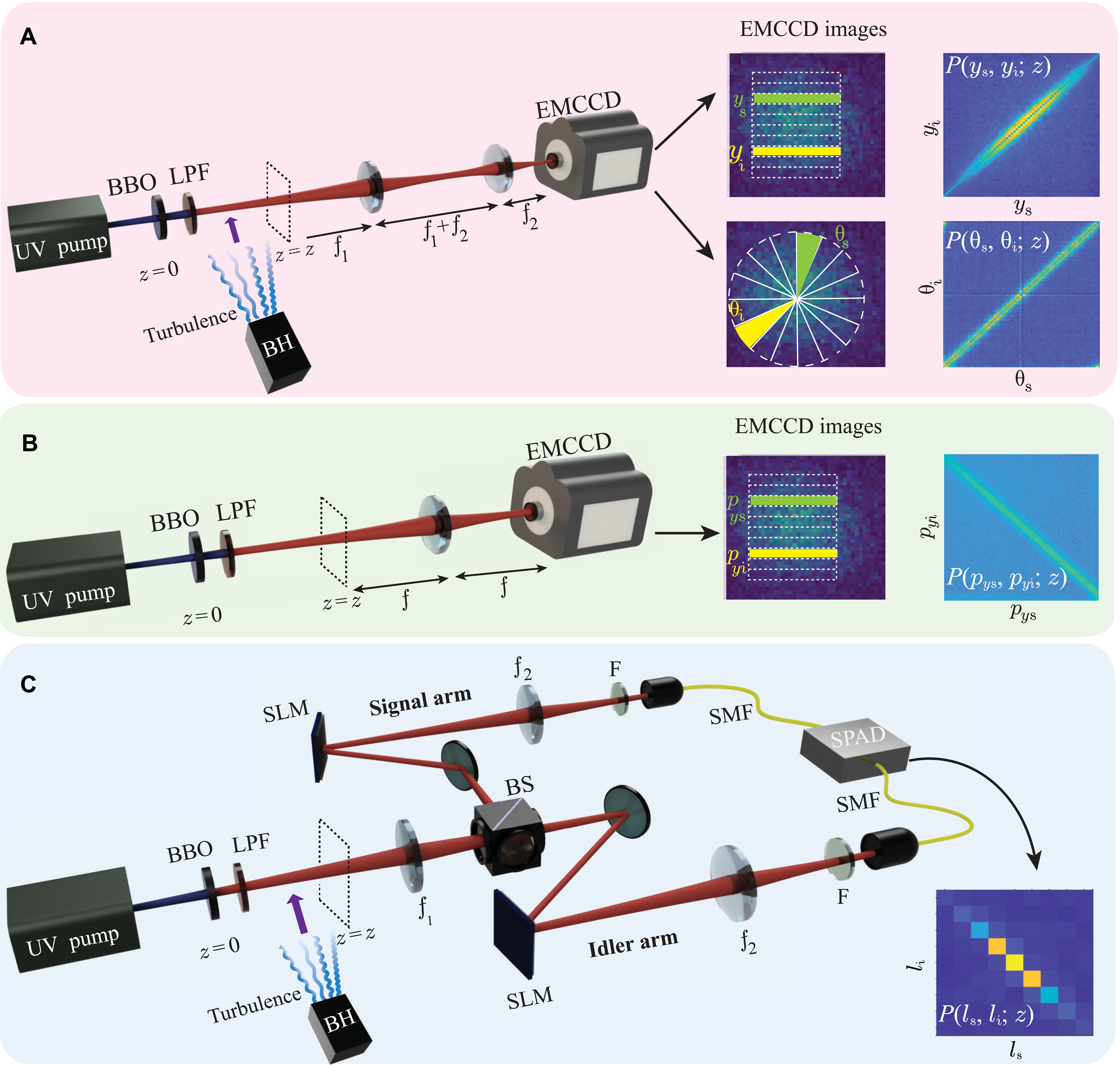
As discussed early, the standard deviation of this probability distribution gives the conditional uncertainty at a distance . Similarly, one can measure the conditional uncertainty in the momentum basis by Fourier transforming equation (VII). In a similar manner, the conditional uncertainty in the angle i.e., is also estimated. Figure 29(a) shows the experimental setup to measure conditional probability in position and angle at distance from the crystal. To measure probability distribution in transverse momentum and OAM of the down-converted photons, setup shown in figure 29(b) and (c) are used respectively.
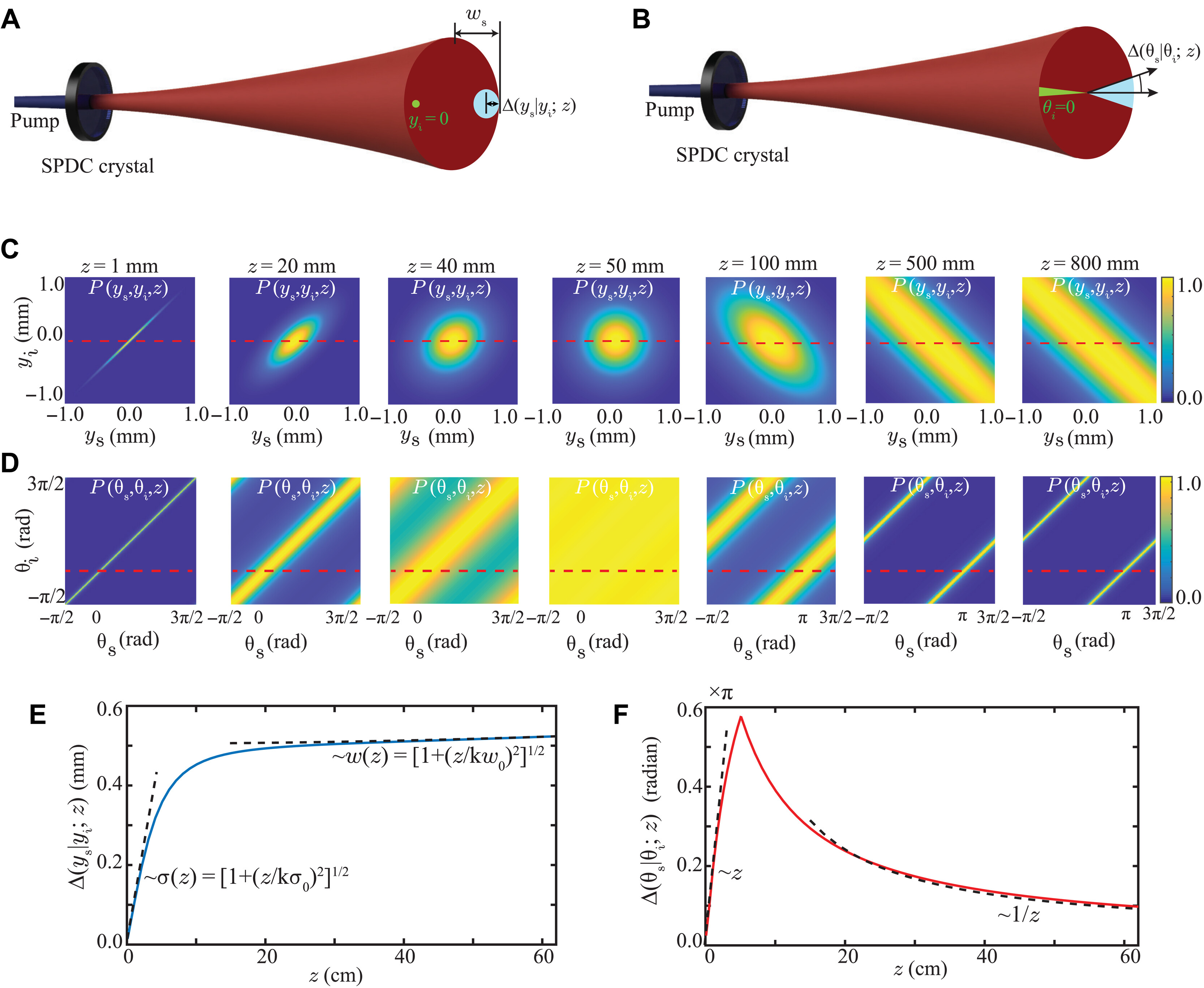
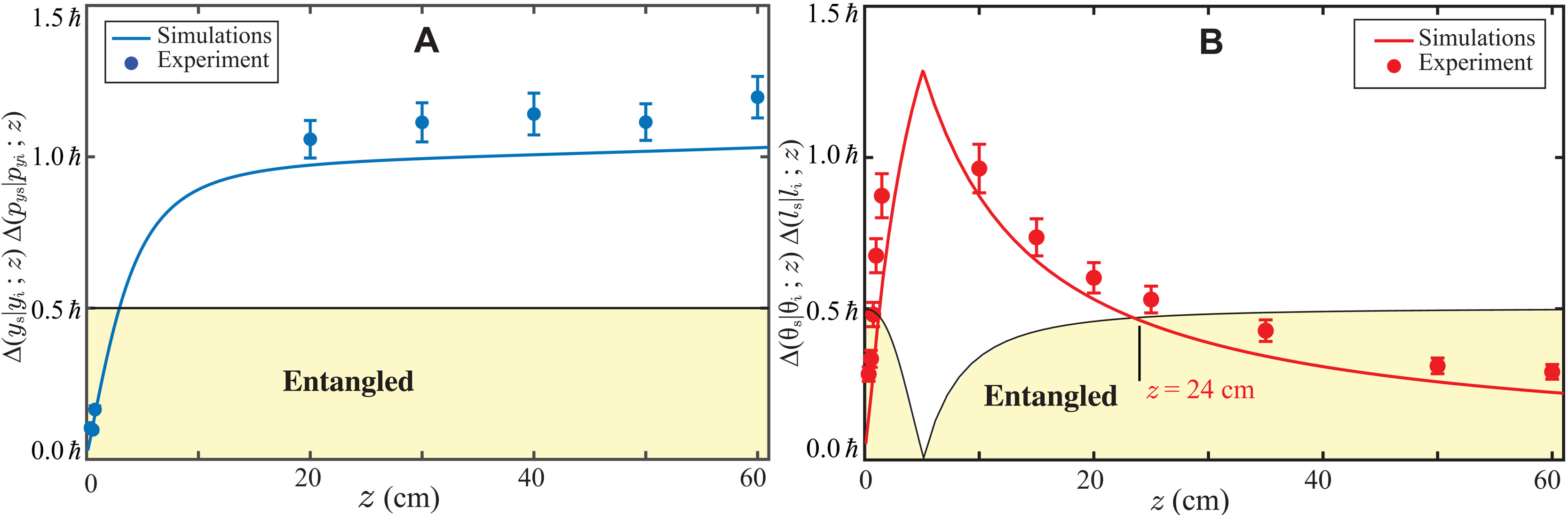
The position and angle evolution of the JPD is depicted in figure 30(c) and (d). By comparing position-JPD and angle-JPD, it becomes evident that the JPD of angle initially broadens until it reaches mm, as does the position JPD. However, relapse to its original JPD size unlike position JPD, which keeps on broadening after mm. Figures 30(e) and (f) shows the numerically calculated conditional uncertainty for position and angle respectively. The figure 30(f) shows the revival of strong angle correlation after further propagation. To measure the conditional probability in OAM basis, two SLMs are used to project the OAM states of two down-converted photons, one reflecting from the beam splitter and another passing through it. The experimental results are shown in figure 30. A product of conditional position-momentum uncertainty against the propagation distance is depicted in figure 30(a), which indicates that after propagating for a given distance from the crystal plane, the entanglement is lost forever. Whereas, results presented in figure 30(b) confirms the revival of the entanglement in angle-OAM bases along the propagation.
VIII Applications of spatial entanglement in the realm of imaging
Spatial correlations have inspired several quantum technological applications, where most of them can be found in the field of quantum imaging. Several reviews on advances in quantum imaging have recently been published [155, 156]. Since the first quantum imaging technique, ghost imaging, this field has flourished, introducing schemes that allow obtaining superresolution [157, 158, 159], supersensitive [160, 161], sub-shot noise imaging [162, 163], holography [164, 165, 166], acquiring images with undetected light [167, 168, 169], and distilling images from stray light [170, 39, 171, 172]. Besides quantum imaging, spatially correlated photons have applications in entanglement distribution [173, 174], quantum communications [175, 176, 177], quantum state engineering, quantum walks [178, 179, 180, 181, 182], and adaptive imaging [183]. In this section, we present some relevant applications of spatial correlations in the realm of imaging.
VIII.1 Ghost imaging
First introduced in 1995 [184, 185], (quantum) ghost imaging was the first imaging method to use spatial correlation of the photon pairs, generated by SPDC. Based on coincidence measurement, one photon of the photon pair interacts with the object (aperture) before getting collected in a fiber while the other photon is collected in a scanning fiber (see figure 31) [185]. Merging the information of coincident photons events and the position of the scanning fiber at that time allows to reconstruct the object in the signal path, resulting in the image shown in figure 32. Instead of a scanning fiber, one can also use a single-photon-sensitive camera [186, 187, 188]. Some other methods also enables to probe the object with a different wavelength than the wavelength detected by the camera, allowing to use more sensitive and less expensive cameras in the visible range while probing an object with a wavelength in the infrared spectrum [189, 190, 191, 192]. Aspden et al. [192] used a BBO-crystal to generate photon pairs at \qty460 and \qty1550, illuminating the object with infrared light before triggering the measurement of the signal photon at an intensified camera with a CCD detector array (ICCD) [192]. To compensate the electrical delay between heralding detector and camera, an image preserving free propagation path was introduced in the signal arm.
Ghost imaging does not necessarily rely on entanglement and can be achieved with classical correlation [193, 194], this is known as classical ghost imaging.
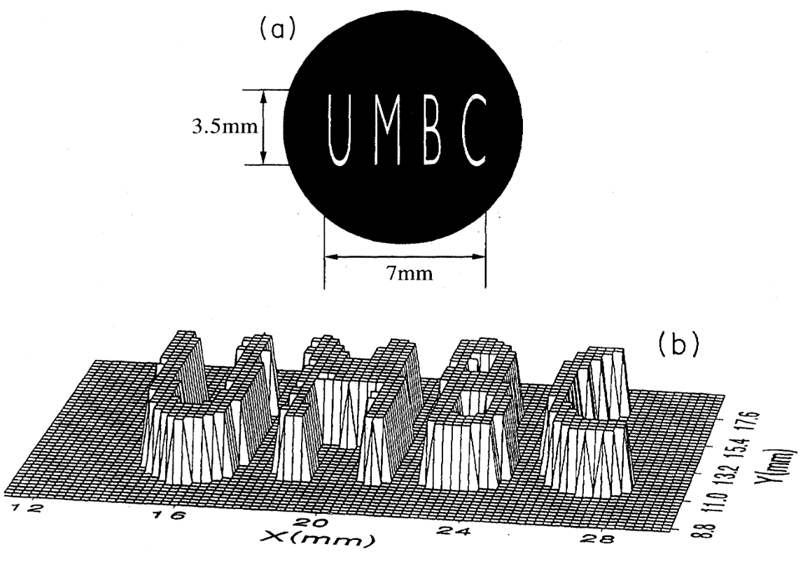
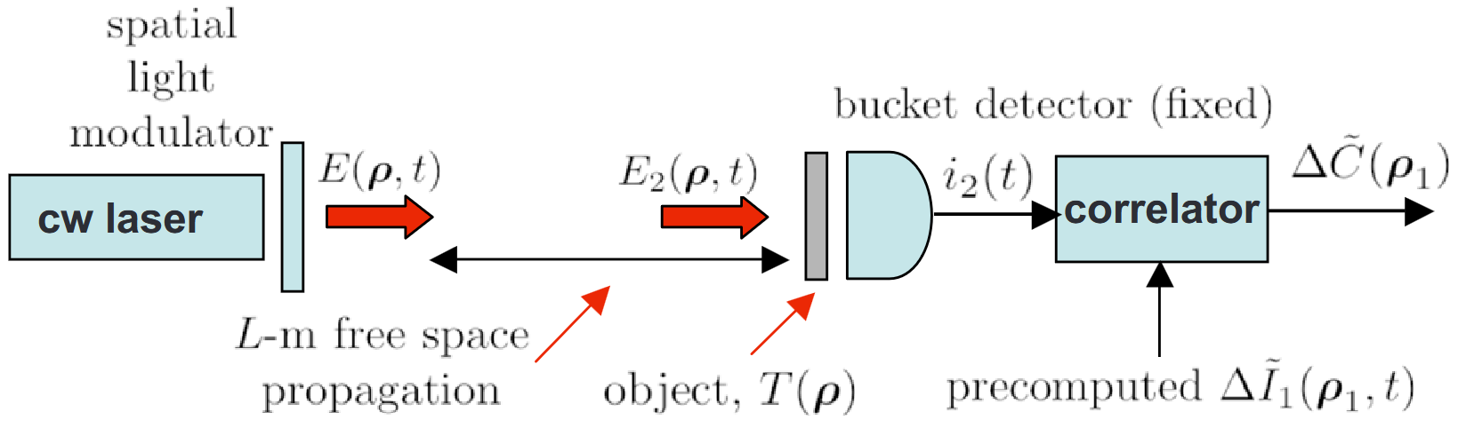
It is also possible to get rid of the camera altogether by using spatially structured light fields [195, 196, 197]. Therefore, the probing arm disappears and a spatial light modulator (SLM/L-m) is inserted into the signal arm as shown in figure 33. The SLM is used to manipulate the light field. Since the pattern of the SLM is well-known, the intensity pattern can be calculated [198]. The acquisition time can be reduced with a reconstruction algorithm based on compressed sensing [199, 200]. This algorithm utilizes redundancies in natural signals to decrease the number of measurements needed for the reconstruction of an object [201].
VIII.2 Quantum image distillation
Classical imaging is vulnerable to stray light and its noise which decreases the quality of the resulting image. Exploiting the characteristics of spatially entangled light, imaging techniques have emerged, using cameras which can measure the spatial correlations of photon pairs [30, 17, 112, 113, 114, 115, 111, 13, 40]
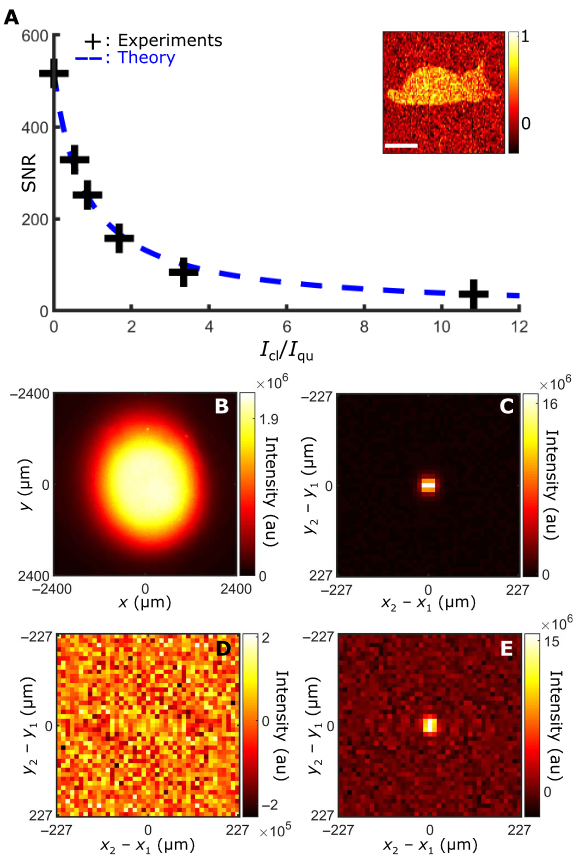
Quantum image distillation allows to separate quantum light consisting of spatially entangled photon pairs from classical light by measuring coincidences using single-photon sensitive EMCCD camera. Here, no prior information about the images is needed, apart from the statistical properties of the illuminating sources, as the quantum image is encoded in correlated photon-pair events. The setup for quantum image distillation is shown in figure 34 [39]. In one arm, spatially correlated photon pairs are generated in a -barium borate (BBO) crystal which illuminate the object (sleeping cat) using two lenses and . In another arm classical light passes through an object (standing cat). Both images are superimposed by an unbalanced beam splitter (92:8) and imaged on an EMCCD camera using a lens , followed by a polarizer and a bandpass filter. As one can see in figure 35(a), both objects are overlapped in the intensity image. Using correlation measurement, the pure quantum image can be made visible in figure 35(b) or by subtracting it from the direct intensity image, one can get the pure classical image of as in figure 35(c). Mathematically, the quantum image is represented by , where is the intensity correlation function and is a camera pixel position. When position-correlated photon pairs illuminates the object , is proportional to it’s shape i.e., . Remainder intensities in the retrieved classical images 35(c) & (f) that are located near the edges can be traced back to absorption of a single photon from a photon pair when propagating through the objects. Signal to noise ratios are measured for minus-coordinate projection of which represents the probability of coincidence of two pair photons at pixels separated by distance -, as shown in figure 36(c) and (e). Figure 36(a) illustrates that the signal-to-noise ratio (SNR) decreases, as the ratio of average intensities between classical and quantum illumination () increases. Figures 36(c) and 36(e) display the negative-coordinate projections of at = 0 and = 11, respectively. The central peaks are then clear indications of strong position correlation between photon pairs. For, =, these peaks vanishes. This technique is robust because over a wide range of classical illumination, even when it is 10x higher than the quantum illumination, SNR1 is maintained.
This image distillation scheme has already been expanded to full-field imaging [202, 41]. While Gregory et al. [202] the resilience of their detection protocol to environmental noise and transmission losses compared to prior quantum illumination protocols, Defienne et al. [41] used a SPAD camera proving their worth in various fields including quantum imaging in a robust scheme against stray light.
VIII.3 Pixel-super-resolution imaging
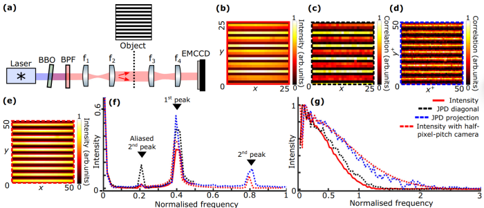
Due to the presence of strong position correlations in photon pairs, this can be leveraged to achieve pixel super-resolution, as outlined in the article [40]. There they demonstrated a quantum image processing technique that increases the pixel resolution by a factor two. The experimental setup is shown in the figure 38(a), where entangled photons are generated using type-1 BBO crystal. The crystal plane is imaged onto an object which is a square-modulation amplitude grating. Then the object is imaged on the camera with pixel pitch 32 m, the estimated correlation width at the camera plane is =13 m.
In the most of the pair-based imaging schemes, diagonal component of JPD, is used to reconstruct the image of the object i.e., [203, 39, 204, 42]. In figure 38(b) is the direct intensity image, 38(c) is the diagonal component of the JPD image which appears same as direct intensity image, proving no benefits of using diagonal component of JPD i.e., Moire pattern is still present. However, using an another way to retrieve the image of the object without the diagonal component of JPD is possible. For this one can project the JPD along its sum-coordinate axis, achieved by summing 41. Such projection retrieves the image of the object with pixel resolution increased by
| (41) |
where, are the number of pixels of the illuminated region, is the sum-coordinate projection of the JPD and () sum-coordinate pixel indices. Because of the pixel-super resolution, one can see that the spurious low frequency modulation has been removed and the 10 grating periods are now visible. This high resolution image is very similar to the a direct intensity image acquired using a camera with 16 m pixel pitch.
VIII.4 Hiding images in quantum correlations
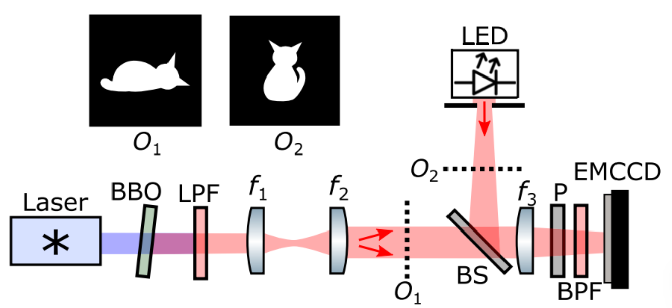
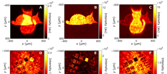
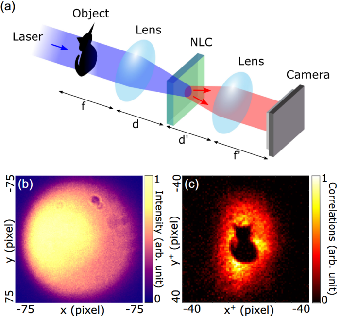
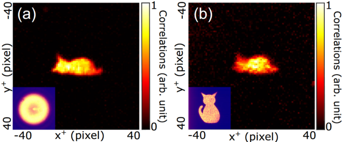
The transfer of information of the pump’s angular spectrum to the SPDC photon pairs have been studied by [89]. This information transfer allows one to control the transverse correlation properties of the down-converted fields by manipulating the pump field. Recently, C. Vernière and H. Defienne [95] presented more generalized study of the transfer of coherence and the phase of the pump beam to the SPDC photon pairs. The experimental setup is shown in figure 38. In the setup, and arbitrary shaped opaque object was inserted in the pump beam and Fourier imaged on the crystal. The Fourier spectrum of a given object gets projected onto a thin nonlinear crystal. Then, the crystal plane is Fourier-imaged onto an EMCCD camera by lens. The direct intensity image of the crystal at far-field is nothing but the just uniform SPDC output as shown in figure 38(b), where as, the intensity correlation image reveals the shape of standing cat as same as the object inserted in pump beam, as shown in figure 38(c). For the next step, authors introduce transparent sleeping cat mask in the pump beam and standing cat mask between and . Lenses and are introduced after lens for Fourier imaging crystal plane on the camera. This time the direct intensity image is of that image of standing cat (figure 39(a) while the intensity correlation image is of that sleeping cat (figure 39(b)). Author’s approach operates for the phase objects as well.
IX Summary and Perspectives
Spatial entanglement in position and momentum has become one of the most versatile resources in quantum optics. Over the past few decades, the theoretical groundwork established by early studies on the Einstein–Podolsky–Rosen (EPR) paradox has led to numerous experimental advancements, confirming the genuine nonlocality of spatially entangled photon pairs generated by spontaneous parametric down-conversion (SPDC). From fundamental tests of quantum realism to application-oriented demonstrations such as quantum imaging, ghost imaging, and high-dimensional quantum communication protocols, the field has expanded in both scope and sophistication.
A salient feature of position-momentum entanglement is its inherently high dimensionality, which provides practical advantages in encoding large amounts of quantum information and enhancing noise resilience. Various approaches have been introduced to quantify, certify, and fully characterize these correlations. Traditional slit-based coincidences provided some of the earliest evidence for EPR violations, while more recent techniques utilize cameras (EMCCDs, SPAD arrays) that capture entire two-dimensional joint probability distributions in real time. These camera-based techniques have significantly reduced acquisition times and opened the door to studies of dynamic or non-ideal conditions, making spatial entanglement measurements increasingly robust and accessible.
Control over the spatial coherence and transverse profile of the pump beam has emerged as a powerful method for tailoring the entanglement properties of SPDC photons. By tuning key parameters—crystal length, beam waist, wavelength, and phase-matching conditions—one can manage the position or momentum correlation widths, thereby shaping the trade-offs between resolution, brightness, and degree of entanglement. Research on partially coherent pumps and wavefront-shaping in SPDC underscores the potential for “engineered” entanglement, allowing one to design custom correlations for specialized applications, from advanced holography to sensor fusion in turbulent environments.
Despite these achievements, challenges persist. Long-distance free-space transmission of spatially entangled photons, for instance, faces hurdles such as diffraction, turbulence, and scattering. Exploring the limits of entanglement transport and developing protocols for entanglement distillation or error correction will be essential steps in converting laboratory-scale demonstrations into robust quantum networks. Integration with waveguide photonics remains a promising frontier, as it can provide stability, scalability, and synergy with cutting-edge on-chip devices.
Looking ahead, the interplay of spatial entanglement, quantum metrology, and machine learning may lead to new protocols capable of extracting detailed sample information from minimal photon resources. Meanwhile, harnessing high-dimensional OAM-based or hybrid (polarization-plus-spatial) states will expand the capacity of future quantum communication channels. As research progresses, one can anticipate more sophisticated entanglement sources, faster and more sensitive detection schemes, and increasingly advanced quantum-optical architectures designed around the unique strengths of position-momentum entanglement. Together, these advancements promise to deepen our fundamental understanding of nonlocality while accelerating the deployment of quantum technologies across a wide range of scientific and industrial fields.
X Acknowledgment
The authors acknowledge financial support from the German Federal Ministry of Education and Research (BMBF) within the funding program “quantum technologies—from basic research to market” with contract number 13N16496 (QUANCER) and from the German Research Foundation (DFG) under the project number 552245798.
XI Conflict of Interest
The authors declare no conflict of interest.
XII Keywords
spatial entanglement, position-momentum entanglement, quantum imaging
References
- Einstein et al. [1935] A. Einstein, B. Podolsky, and N. Rosen, Can quantum-mechanical description of physical reality be considered complete?, Phys. Rev. 47, 777 (1935).
- Schrödinger [1935] E. Schrödinger, Discussion of probability relations between separated systems, Mathematical Proceedings of the Cambridge Philosophical Society 31, 555–563 (1935).
- Bohm and Aharonov [1957] D. Bohm and Y. Aharonov, Discussion of experimental proof for the paradox of einstein, rosen, and podolsky, Phys. Rev. 108, 1070 (1957).
- Bell [1964] J. S. Bell, On the einstein podolsky rosen paradox, Physics Physique Fizika 1, 195 (1964).
- Cirel’son [1980] B. S. Cirel’son, Quantum generalizations of bell’s inequality, Letters in Mathematical Physics 4, 93 (1980).
- Clauser et al. [1969] J. F. Clauser, M. A. Horne, A. Shimony, and R. A. Holt, Proposed experiment to test local hidden-variable theories, Phys. Rev. Lett. 23, 880 (1969).
- Ekert [1991] A. K. Ekert, Quantum cryptography based on bell’s theorem, Phys. Rev. Lett. 67, 661 (1991).
- Bouwmeester et al. [1997] D. Bouwmeester, J.-W. Pan, K. Mattle, M. Eibl, H. Weinfurter, and A. Zeilinger, Experimental quantum teleportation, Nature 390, 575 (1997).
- Jacak et al. [2020] J. E. Jacak, W. A. Jacak, W. A. Donderowicz, and L. Jacak, Quantum random number generators with entanglement for public randomness testing, Scientific Reports 10, 164 (2020).
- Liu et al. [2018] Y. Liu, X. Yuan, M.-H. Li, W. Zhang, Q. Zhao, J. Zhong, Y. Cao, Y.-H. Li, L.-K. Chen, H. Li, T. Peng, Y.-A. Chen, C.-Z. Peng, S.-C. Shi, Z. Wang, L. You, X. Ma, J. Fan, Q. Zhang, and J.-W. Pan, High-speed device-independent quantum random number generation without a detection loophole, Phys. Rev. Lett. 120, 010503 (2018).
- Matthews et al. [2016] J. C. F. Matthews, X.-Q. Zhou, H. Cable, P. J. Shadbolt, D. J. Saunders, G. A. Durkin, G. J. Pryde, and J. L. O’Brien, Towards practical quantum metrology with photon counting, NPJ Quantum Information 2, 16023 (2016).
- Howell et al. [2004] J. C. Howell, R. S. Bennink, S. J. Bentley, and R. W. Boyd, Realization of the einstein-podolsky-rosen paradox using momentum- and position-entangled photons from spontaneous parametric down conversion, Phys. Rev. Lett. 92, 210403 (2004).
- Defienne et al. [2020] H. Defienne, T. Reichert, Q. Sun, R. S. Aspden, T. Schneider, K. Lee, R. Fickler, G. Leuchs, R. W. Boyd, and C. Silberhorn, Imaging and certifying high-dimensional entanglement with a single-photon avalanche diode camera, npj Quantum Information 6, 1 (2020).
- Leach et al. [2012] J. Leach, R. E. Warburton, D. G. Ireland, F. Izdebski, S. M. Barnett, A. M. Yao, G. S. Buller, and M. J. Padgett, Quantum correlations in position, momentum, and intermediate bases for a full optical field of view, Phys. Rev. A 85, 013827 (2012).
- Achatz et al. [2020] L. Achatz, E. Ortega, K. Dovzhik, R. F. Shiozaki, J. Fuenzalida, S. Wengerowsky, M. Bohmann, and R. Ursin, Certifying position-momentum entanglement at telecommunication wavelengths, Journal of Optics 22, 125201 (2020).
- Zhang et al. [2019] W. Zhang, R. Fickler, E. Giese, L. Chen, and R. W. Boyd, Influence of pump coherence on the generation of position-momentum entanglement in optical parametric down-conversion, Opt. Express 27, 20745 (2019).
- Patil et al. [2023] S. Patil, S. Prabhakar, A. Biswas, A. Kumar, and R. P. Singh, Anisotropic spatial entanglement, Physics Letters A 457, 128583 (2023).
- Franson [1989] J. D. Franson, Bell inequality for position and time, Phys. Rev. Lett. 62, 2205 (1989).
- Xavier et al. [2025] G. B. Xavier, J.- . Larsson, P. Villoresi, G. Vallone, and A. Cabello, Energy-time and time-bin entanglement: past, present and future, arXiv preprint arXiv:2503.14675 (2025), review paper. 27 pages, 9 figures, 250+ references. Comments welcome!
- Shalm et al. [2013a] L. K. Shalm, D. R. Hamel, Z. Yan, C. Simon, K. J. Resch, and T. Jennewein, Three-photon energy–time entanglement, Nature Physics 9, 19 (2013a).
- Ali-Khan et al. [2007] I. Ali-Khan, C. J. Broadbent, and J. C. Howell, Large-alphabet quantum key distribution using energy-time entangled bipartite states, Phys. Rev. Lett. 98, 060503 (2007).
- Strekalov et al. [1996] D. V. Strekalov, T. B. Pittman, A. V. Sergienko, Y. H. Shih, and P. G. Kwiat, Postselection-free energy-time entanglement, Phys. Rev. A 54, R1 (1996).
- Kwiat et al. [1993] P. G. Kwiat, A. M. Steinberg, and R. Y. Chiao, High-visibility interference in a bell-inequality experiment for energy and time, Phys. Rev. A 47, R2472 (1993).
- Ali Khan and Howell [2006] I. Ali Khan and J. C. Howell, Experimental demonstration of high two-photon time-energy entanglement, Phys. Rev. A 73, 031801 (2006).
- Shalm et al. [2013b] L. K. Shalm, D. R. Hamel, Z. Yan, C. Simon, K. J. Resch, and T. Jennewein, Three-photon energy–time entanglement, Nature Physics 9, 19 (2013b).
- Ou et al. [1992a] Z. Y. Ou, S. F. Pereira, H. J. Kimble, and K. C. Peng, Quantum entanglement and squeezing of the quadrature difference of bright light fields, Physical Review Letters 68, 3663 (1992a).
- Doe and Smith [2023] J. Doe and J. Smith, Quadrature entanglement in the microwave domain with a phase locking protocol, Physical Review Letters 130, 060501 (2023).
- Furusawa et al. [1998] A. Furusawa, J. L. Sørensen, S. L. Braunstein, C. A. Fuchs, H. J. Kimble, and E. S. Polzik, Experimental realization of spatially separated entanglement with continuous variables using laser pulse trains, Science 282, 706 (1998).
- Bowen et al. [2003] W. P. Bowen, R. Schnabel, P. K. Lam, and T. C. Ralph, Experimental investigation of criteria for continuous variable entanglement, Phys. Rev. Lett. 90, 043601 (2003).
- Edgar et al. [2012] M. Edgar, D. Tasca, F. Izdebski, R. Warburton, J. Leach, M. Agnew, G. Buller, R. Boyd, and M. Padgett, Imaging high-dimensional spatial entanglement with a camera, Nature Communications 3, 984 (2012).
- Moreau et al. [2014] P.-A. Moreau, F. Devaux, and E. Lantz, Einstein-podolsky-rosen paradox in twin images, Phys. Rev. Lett. 113, 160401 (2014).
- Leach et al. [2010] J. Leach, B. Jack, J. Romero, A. K. Jha, A. M. Yao, S. Franke-Arnold, D. G. Ireland, R. W. Boyd, S. M. Barnett, and M. J. Padgett, Quantum correlations in optical angle–orbital angular momentum variables, Science 329, 662 (2010), https://www.science.org/doi/pdf/10.1126/science.1190523 .
- Rastegin [2017] A. E. Rastegin, Rényi formulation of entanglement criteria for continuous variables, Phys. Rev. A 95, 042334 (2017).
- Saboia et al. [2011] A. Saboia, F. Toscano, and S. P. Walborn, Family of continuous-variable entanglement criteria using general entropy functions, Phys. Rev. A 83, 032307 (2011).
- Giedke et al. [2001] G. Giedke, B. Kraus, M. Lewenstein, and J. I. Cirac, Entanglement criteria for all bipartite gaussian states, Phys. Rev. Lett. 87, 167904 (2001).
- Simon [2000] R. Simon, Peres-horodecki separability criterion for continuous variable systems, Phys. Rev. Lett. 84, 2726 (2000).
- Scarfe et al. [2025] L. Scarfe, Y. Zhang, and E. Karimi, Spatial-mode quantum cryptography in a 545-dimensional hilbert space (2025), arXiv:2503.22058 [quant-ph] .
- Braunstein and Kimble [1998] S. L. Braunstein and H. J. Kimble, Teleportation of continuous quantum variables, Phys. Rev. Lett. 80, 869 (1998).
- Defienne et al. [2019] H. Defienne, M. Reichert, J. W. Fleischer, and D. Faccio, Quantum image distillation, Science Advances 5, eaax0307 (2019), https://www.science.org/doi/pdf/10.1126/sciadv.aax0307 .
- Defienne et al. [2022a] H. Defienne, P. Cameron, B. Ndagano, A. Lyons, M. Reichert, J. Zhao, A. R. Harvey, E. Charbon, J. W. Fleischer, and D. Faccio, Pixel super-resolution with spatially entangled photons, Nature Communications 13, 3566 (2022a).
- Defienne et al. [2021a] H. Defienne, J. Zhao, E. Charbon, and D. Faccio, Full-field quantum imaging with a single-photon avalanche diode camera, Phys. Rev. A 103, 042608 (2021a).
- Reichert et al. [2017a] M. Reichert, H. Defienne, X. Sun, and J. W. Fleischer, Biphoton transmission through non-unitary objects, Journal of Optics 19, 034013 (2017a).
- Ndagano and Faccio [2022] B. Ndagano and D. Faccio, Quantum microscopy based on hong–ou–mandel interference, Nature Communications 13, 1215 (2022).
- Moreau et al. [2018a] P.-A. Moreau, E. Toninelli, P. A. Morris, R. S. Aspden, T. Gregory, G. Spalding, R. W. Boyd, and M. J. Padgett, Resolution limits of quantum ghost imaging, Opt. Express 26, 7528 (2018a).
- Fuenzalida et al. [2022] J. Fuenzalida, A. Hochrainer, G. B. Lemos, E. A. Ortega, R. Lapkiewicz, M. Lahiri, and A. Zeilinger, Resolution of quantum imaging with undetected photons, Quantum 6, 646 (2022).
- Viswanathan et al. [2021] B. Viswanathan, G. Barreto Lemos, and M. Lahiri, Resolution limit in quantum imaging with undetected photons using position correlations, Optics Express 29, 38185 (2021).
- Vega et al. [2022] A. Vega, E. A. Santos, J. Fuenzalida, M. Gilaberte Basset, T. Pertsch, M. Gräfe, S. Saravi, and F. Setzpfandt, Fundamental resolution limit of quantum imaging with undetected photons, Physical Review Research 4, 033252 (2022).
- Gilaberte Basset et al. [2023] M. Gilaberte Basset, R. Sondenheimer, J. Fuenzalida, A. Vega, S. Töpfer, E. A. Santos, S. Saravi, F. Setzpfandt, F. Steinlechner, and M. Gräfe, Experimental analysis of image resolution of quantum imaging with undetected light through position correlations, Physical Review A 108, 052610 (2023).
- Giovannetti et al. [2011] V. Giovannetti, S. Lloyd, and L. Maccone, Advances in quantum metrology, Nature Photonics 5, 222 (2011).
- Giovannetti et al. [2006] V. Giovannetti, S. Lloyd, and L. Maccone, Quantum metrology, Phys. Rev. Lett. 96, 010401 (2006).
- Aspect et al. [1981] A. Aspect, P. Grangier, and G. Roger, Experimental tests of realistic local theories via bell’s theorem, Phys. Rev. Lett. 47, 460 (1981).
- Aspect et al. [1982] A. Aspect, J. Dalibard, and G. Roger, Experimental test of bell’s inequalities using time-varying analyzers, Phys. Rev. Lett. 49, 1804 (1982).
- Kocher and Commins [1967] C. A. Kocher and E. D. Commins, Polarization correlation of photons emitted in an atomic cascade, Phys. Rev. Lett. 18, 575 (1967).
- Louisell et al. [1961] W. H. Louisell, A. Yariv, and A. E. Siegman, Quantum fluctuations and noise in parametric processes. i., Phys. Rev. 124, 1646 (1961).
- Giallorenzi and Tang [1968] T. G. Giallorenzi and C. L. Tang, Quantum theory of spontaneous parametric scattering of intense light, Phys. Rev. 166, 225 (1968).
- Harris et al. [1967] S. E. Harris, M. K. Oshman, and R. L. Byer, Observation of tunable optical parametric fluorescence, Phys. Rev. Lett. 18, 732 (1967).
- Burnham and Weinberg [1970] D. C. Burnham and D. L. Weinberg, Observation of simultaneity in parametric production of optical photon pairs, Phys. Rev. Lett. 25, 84 (1970).
- Hanbury Brown and Twiss [1956] R. Hanbury Brown and R. Q. Twiss, A test of a new type of stellar interferometer on sirius, Nature 178, 1046 (1956).
- Boyd [2008] R. W. Boyd, Nonlinear Optics, 3rd ed. (Academic Press, 2008).
- Rubin et al. [1994] M. H. Rubin, D. N. Klyshko, Y. H. Shih, and A. V. Sergienko, Theory of two-photon entanglement in type-ii optical parametric down-conversion, Phys. Rev. A 50, 5122 (1994).
- Kwiat et al. [1994] P. G. Kwiat, P. H. Eberhard, A. M. Steinberg, and R. Y. Chiao, Proposal for a loophole-free bell inequality experiment, Phys. Rev. A 49, 3209 (1994).
- Kwiat et al. [1995] P. G. Kwiat, K. Mattle, H. Weinfurter, A. Zeilinger, A. V. Sergienko, and Y. Shih, New high-intensity source of polarization-entangled photon pairs, Phys. Rev. Lett. 75, 4337 (1995).
- Kwiat et al. [1999] P. G. Kwiat, E. Waks, A. G. White, I. Appelbaum, and P. H. Eberhard, Ultrabright source of polarization-entangled photons, Phys. Rev. A 60, R773 (1999).
- Rarity and Tapster [1990] J. G. Rarity and P. R. Tapster, Experimental violation of bell’s inequality based on phase and momentum, Phys. Rev. Lett. 64, 2495 (1990).
- Mair et al. [2001] A. Mair, A. Vaziri, G. Weihs, and A. Zeilinger, Entanglement of the orbital angular momentum states of photons, Nature 412, 313 (2001).
- Law and Eberly [2004a] C. K. Law and J. H. Eberly, Analysis and interpretation of high transverse entanglement in optical parametric down conversion, Phys. Rev. Lett. 92, 127903 (2004a).
- Walborn and Monken [2007] S. P. Walborn and C. H. Monken, Transverse spatial entanglement in parametric down-conversion, Phys. Rev. A 76, 062305 (2007).
- Armstrong et al. [1962] J. A. Armstrong, N. Bloembergen, J. Ducuing, and P. S. Pershan, Interactions between Light Waves in a Nonlinear Dielectric, Physical Review 127, 1918 (1962), publisher: American Physical Society.
- Mattle et al. [1996] K. Mattle, H. Weinfurter, P. G. Kwiat, and A. Zeilinger, Dense coding in experimental quantum communication, Phys. Rev. Lett. 76, 4656 (1996).
- Bennett et al. [1992] C. H. Bennett, G. Brassard, and N. D. Mermin, Quantum cryptography without bell’s theorem, Phys. Rev. Lett. 68, 557 (1992).
- Wootters and Zurek [1982] W. K. Wootters and W. H. Zurek, A single quantum cannot be cloned, Nature 299, 802 (1982).
- Beth [1936] R. A. Beth, Mechanical detection and measurement of the angular momentum of light, Phys. Rev. 50, 115 (1936).
- Padgett et al. [2004] M. Padgett, J. Courtial, and L. Allen, Light’s Orbital Angular Momentum, Physics Today 57, 35 (2004), https://pubs.aip.org/physicstoday/article-pdf/57/5/35/8317006/35_1_online.pdf .
- Molina-Terriza et al. [2007] G. Molina-Terriza, J. P. Torres, and L. Torner, Twisted photons, Nature Physics 3, 305 (2007).
- Brandt et al. [2020] F. Brandt, M. Hiekkamäki, F. Bouchard, M. Huber, and R. Fickler, High-dimensional quantum gates using full-field spatial modes of photons, Optica 7, 98 (2020).
- Anwar et al. [2021] A. Anwar, S. Prabhakar, and R. P. Singh, Size-invariant twisted optical modes for the efficient generation of higher-dimensional quantum states, J. Opt. Soc. Am. B 38, 2976 (2021).
- Karimipour et al. [2002] V. Karimipour, A. Bahraminasab, and S. Bagherinezhad, Entanglement swapping of generalized cat states and secret sharing, Physical Review A 65, 042320 (2002).
- Bechmann-Pasquinucci and Peres [2000] H. Bechmann-Pasquinucci and A. Peres, Quantum cryptography with 3-state systems, Physical Review Letters 85, 3313 (2000).
- Molina-Terriza et al. [2001] G. Molina-Terriza, J. P. Torres, and L. Torner, Management of the angular momentum of light: Preparation of photons in multidimensional vector states of angular momentum, Phys. Rev. Lett. 88, 013601 (2001).
- Vaziri et al. [2002] A. Vaziri, G. Weihs, and A. Zeilinger, Experimental two-photon, three-dimensional entanglement for quantum communication, Phys. Rev. Lett. 89, 240401 (2002).
- Torres et al. [2003] J. P. Torres, Y. Deyanova, L. Torner, and G. Molina-Terriza, Preparation of engineered two-photon entangled states for multidimensional quantum information, Phys. Rev. A 67, 052313 (2003).
- Anwar et al. [2020] A. Anwar, N. Lal, S. Prabhakar, and R. P. Singh, Selective tuning of hilbert spaces in states encoded with spatial modes of light, New Journal of Physics 22, 113020 (2020).
- Jabir et al. [2019] M. V. Jabir, A. Anwar, and G. K. Samanta, Controlling the bi-photon orbital angular momentum eigenmodes using asymmetric pump vortex beam, Journal of Optics 21, 055201 (2019).
- Reid and Drummond [1988] M. D. Reid and P. D. Drummond, Quantum correlations of phase in nondegenerate parametric oscillation, Phys. Rev. Lett. 60, 2731 (1988).
- Ou et al. [1992b] Z. Y. Ou, S. F. Pereira, H. J. Kimble, and K. C. Peng, Realization of the einstein-podolsky-rosen paradox for continuous variables, Phys. Rev. Lett. 68, 3663 (1992b).
- Duan et al. [2000] L.-M. Duan, G. Giedke, J. I. Cirac, and P. Zoller, Inseparability criterion for continuous variable systems, Phys. Rev. Lett. 84, 2722 (2000).
- Strekalov et al. [1995a] D. V. Strekalov, A. V. Sergienko, D. N. Klyshko, and Y. H. Shih, Observation of two-photon “ghost” interference and diffraction, Phys. Rev. Lett. 74, 3600 (1995a).
- Pittman et al. [1995a] T. B. Pittman, Y. H. Shih, D. V. Strekalov, and A. V. Sergienko, Optical imaging by means of two-photon quantum entanglement, Phys. Rev. A 52, R3429 (1995a).
- Monken et al. [1998] C. H. Monken, P. H. S. Ribeiro, and S. Pádua, Transfer of angular spectrum and image formation in spontaneous parametric down-conversion, Phys. Rev. A 57, 3123 (1998).
- Abouraddy et al. [2001] A. F. Abouraddy, M. B. Nasr, B. E. A. Saleh, A. V. Sergienko, and M. C. Teich, Demonstration of the complementarity of one- and two-photon interference, Phys. Rev. A 63, 063803 (2001).
- Walborn et al. [2006] S. P. Walborn, D. S. Lemelle, M. P. Almeida, and P. H. S. Ribeiro, Quantum key distribution with higher-order alphabets using spatially encoded qudits, Phys. Rev. Lett. 96, 090501 (2006).
- Walborn et al. [2008] S. P. Walborn, D. S. Lemelle, D. S. Tasca, and P. H. Souto Ribeiro, Schemes for quantum key distribution with higher-order alphabets using single-photon fractional fourier optics, Phys. Rev. A 77, 062323 (2008).
- Defienne and Gigan [2019a] H. Defienne and S. Gigan, Spatially entangled photon-pair generation using a partial spatially coherent pump beam, Phys. Rev. A 99, 053831 (2019a).
- Boucher et al. [2021] P. Boucher, H. Defienne, and S. Gigan, Engineering spatial correlations of entangled photon pairs by pump beam shaping, Opt. Lett. 46, 4200 (2021).
- Vernière and Defienne [2024] C. Vernière and H. Defienne, Hiding Images in Quantum Correlations, Physical Review Letters 133, 093601 (2024).
- Reichert et al. [2017b] M. Reichert, X. Sun, and J. W. Fleischer, Quality of spatial entanglement propagation, Phys. Rev. A 95, 063836 (2017b).
- Bhattacharjee et al. [2022a] A. Bhattacharjee, M. K. Joshi, S. Karan, J. Leach, and A. K. Jha, Propagation-induced revival of entanglement in the angle-oam bases, Science Advances 8, eabn7876 (2022a), https://www.science.org/doi/pdf/10.1126/sciadv.abn7876 .
- Chan et al. [2007a] K. W. Chan, J. P. Torres, and J. H. Eberly, Transverse entanglement migration in hilbert space, Phys. Rev. A 75, 050101 (2007a).
- Tasca et al. [2009] D. S. Tasca, S. P. Walborn, P. H. Souto Ribeiro, F. Toscano, and P. Pellat-Finet, Propagation of transverse intensity correlations of a two-photon state, Phys. Rev. A 79, 033801 (2009).
- Friis et al. [2019] N. Friis, G. Vitagliano, M. Malik, and M. Huber, Entanglement certification from theory to experiment, Nat. Rev. Phys. 1, 72 (2019).
- Brambilla et al. [2004] E. Brambilla, A. Gatti, M. Bache, and L. A. Lugiato, Simultaneous near-field and far-field spatial quantum correlations in the high-gain regime of parametric down-conversion, Phys. Rev. A 69, 023802 (2004).
- Kviatkovsky et al. [2020] I. Kviatkovsky, H. M. Chrzanowski, E. G. Avery, H. Bartolomaeus, and S. Ramelow, Microscopy with undetected photons in the mid-infrared, Sci. Adv. 6, eabd0264 (2020).
- Hong et al. [2024] M. Hong, R. Gómez, V. Flavio Gili, J. Fuenzalida, and M. Gräfe, Polarization-entangled photon-pair source using beam displacers and thin crystals, Opt. Lett. 49, 5467 (2024).
- Law and Eberly [2004b] C. K. Law and J. H. Eberly, Analysis and interpretation of high transverse entanglement in optical parametric down conversion, Phys. Rev. Lett. 92, 127903 (2004b).
- Di Lorenzo Pires et al. [2009a] H. Di Lorenzo Pires, C. H. Monken, and M. P. van Exter, Direct measurement of transverse-mode entanglement in two-photon states, Phys. Rev. A 80, 022307 (2009a).
- Ortega et al. [2022] E. A. Ortega, J. Fuenzalida, M. Selimovic, K. Dovzhik, L. Achatz, S. Wengerowsky, R. F. Shiozaki, S. P. Neumann, M. Bohmann, and R. Ursin, Spatial and spectral characterization of photon pairs at telecommunication wavelengths from type-0 spontaneous parametric downconversion, J. Opt. Soc. Am. B 40, 165 (2022).
- Just et al. [2013] F. Just, A. Cavanna, M. V. Chekhova, and G. Leuchs, Transverse entanglement of biphotons, New J. Phys. 15, 083015 (2013).
- Brida et al. [2009] G. Brida, V. Caricato, M. Fedorov, M. Genovese, M. Gramegna, and S. Kulik, Characterization of spectral entanglement of spontaneous parametric-down conversion biphotons in femtosecond pulsed regime, EPL 87, 64003 (2009).
- Fedorov et al. [2004] M. V. Fedorov, M. A. Efremov, A. E. Kazakov, K. W. Chan, C. K. Law, and J. H. Eberly, Packet narrowing and quantum entanglement in photoionization and photodissociation, Phys. Rev. A 69, 052117 (2004).
- Chan et al. [2007b] K. W. Chan, J. P. Torres, and J. H. Eberly, Transverse entanglement migration in hilbert space, Phys. Rev. A 75, 050101 (2007b).
- Defienne et al. [2018a] H. Defienne, M. Reichert, and J. W. Fleischer, General model of photon-pair detection with an image sensor, Phys. Rev. Lett. 120, 203604 (2018a).
- Eckmann et al. [2020] B. Eckmann, B. Bessire, M. Unternährer, L. Gasparini, M. Perenzoni, and A. Stefanov, Characterization of space-momentum entangled photons with a time resolving cmos spad array, Opt. Express 28, 31553 (2020).
- Kundu et al. [2024] S. Kundu, J. Szuniewicz, G. Firlik, A. Krupinski-Ptaszek, and R. Lapkiewicz, High-dimensional quantum correlation measurements with an adaptively gated hybrid single-photon camera, Optica Quantum 2, 206 (2024).
- Courme et al. [2023] B. Courme, C. Vernière, P. Svihra, S. Gigan, A. Nomerotski, and H. Defienne, Quantifying high-dimensional spatial entanglement with a single-photon-sensitive time-stamping camera, Opt. Lett. 48, 3439 (2023).
- Severini et al. [2023] F. Severini, I. Cusini, F. Madonini, D. Brescia, R. Camphausen, A. Cuevas, S. Tisa, and F. Villa, Spatially resolved event-driven 24 x 24 pixels spad imager with 100 % duty cycle for low optical power quantum entanglement detection, IEEE Journal of Solid-State Circuits 58, 2278 (2023).
- Reichert et al. [2018a] M. Reichert, H. Defienne, and J. W. Fleischer, Optimizing the signal-to-noise ratio of biphoton distribution measurements, Phys. Rev. A 98, 013841 (2018a).
- Defienne et al. [2022b] H. Defienne, P. Cameron, B. Ndagano, A. Lyons, M. Reichert, J. Zhao, A. R. Harvey, E. Charbon, J. W. Fleischer, and D. Faccio, Pixel super-resolution with spatially entangled photons, Nature Communications 13, 3566 (2022b).
- Rochas et al. [2003] A. Rochas, M. Gosch, A. Serov, P. Besse, R. Popovic, T. Lasser, and R. Rigler, First fully integrated 2-d array of single-photon detectors in standard cmos technology, IEEE Photonics Technology Letters 15, 963 (2003).
- Bronzi et al. [2014] D. Bronzi, F. Villa, S. Tisa, A. Tosi, F. Zappa, D. Durini, S. Weyers, and W. Brockherde, 100 000 frames/s 64 × 32 single-photon detector array for 2-d imaging and 3-d ranging, IEEE Journal of Selected Topics in Quantum Electronics 20, 355 (2014).
- Lindner et al. [2018] S. Lindner, C. Zhang, I. M. Antolovic, M. Wolf, and E. Charbon, A 252 × 144 spad pixel flash lidar with 1728 dual-clock 48.8 ps tdcs, integrated histogramming and 14.9-to-1 compression in 180nm cmos technology, in 2018 IEEE Symposium on VLSI Circuits (2018) pp. 69–70.
- Henderson et al. [2019] R. K. Henderson, N. Johnston, S. W. Hutchings, I. Gyongy, T. A. Abbas, N. Dutton, M. Tyler, S. Chan, and J. Leach, 5.7 a 256×256 40nm/90nm cmos 3d-stacked 120db dynamic-range reconfigurable time-resolved spad imager, in 2019 IEEE International Solid-State Circuits Conference - (ISSCC) (2019) pp. 106–108.
- Bruschini et al. [2020] C. Bruschini, H. Homulle, I. M. Antolovic, S. Burri, and E. Charbon, Author correction: Single-photon avalanche diode imagers in biophotonics: review and outlook, Light: Science & Applications 9, 12 (2020), an amendment to this paper has been published and can be accessed via a link at the top of the paper.
- Li et al. [2010] D.-U. Li, J. Arlt, J. Richardson, R. Walker, A. Buts, D. Stoppa, E. Charbon, and R. Henderson, Real-time fluorescence lifetime imaging system with a 32 × 32 0.13m cmos low dark-count single-photon avalanche diode array, Opt. Express 18, 10257 (2010).
- Henderson et al. [2018] R. K. Henderson, N. Johnston, H. Chen, D. D.-U. Li, G. Hungerford, R. Hirsch, D. McLoskey, P. Yip, and D. J. Birch, A 192×128 time correlated single photon counting imager in 40nm cmos technology, in ESSCIRC 2018 - IEEE 44th European Solid State Circuits Conference (ESSCIRC) (2018) pp. 54–57.
- Lyons et al. [2019] A. Lyons, F. Tonolini, A. Boccolini, A. Repetti, R. Henderson, Y. Wiaux, and D. Faccio, Computational time-of-flight diffuse optical tomography, Nature Photonics 13, 575 (2019).
- Gariepy et al. [2016] G. Gariepy, F. Tonolini, R. Henderson, J. Leach, and D. Faccio, Detection and tracking of moving objects hidden from view, Nature Photonics 10, 23 (2016).
- Lubin et al. [2019] G. Lubin, R. Tenne, I. M. Antolovic, E. Charbon, C. Bruschini, and D. Oron, Quantum correlation measurement with single photon avalanche diode arrays, Opt. Express 27, 32863 (2019).
- Unternährer et al. [2016] M. Unternährer, B. Bessire, L. Gasparini, D. Stoppa, and A. Stefanov, Coincidence detection of spatially correlated photon pairs with a monolithic time-resolving detector array, Opt. Express 24, 28829 (2016).
- Bavaresco et al. [2018] J. Bavaresco, N. Herrera Valencia, C. Klöckl, M. Pivoluska, P. Erker, N. Friis, M. Malik, and M. Huber, Measurements in two bases are sufficient for certifying high-dimensional entanglement, Nature Physics 14, 1032 (2018).
- Schneeloch et al. [2019] J. Schneeloch, C. C. Tison, M. L. Fanto, P. M. Alsing, and G. A. Howland, Quantifying entanglement in a 68-billion-dimensional quantum state space, Nature Communications 10, 2785 (2019).
- Valencia et al. [2020a] N. H. Valencia, S. Goel, W. McCutcheon, H. Defienne, and M. Malik, Unscrambling entanglement through a complex medium, Nature Physics 16, 1112 (2020a).
- Bhattacharjee et al. [2022b] A. Bhattacharjee, N. Meher, and A. K. Jha, Measurement of two-photon position–momentum einstein–podolsky–rosen correlations through single-photon intensity measurements, New Journal of Physics 24, 053033 (2022b).
- Jha et al. [2011] A. K. Jha, G. S. Agarwal, and R. W. Boyd, Partial angular coherence and the angular schmidt spectrum of entangled two-photon fields, Phys. Rev. A 84, 063847 (2011).
- Kulkarni and Jha [2017] G. Kulkarni and A. K. Jha, Single-shot measurement of the orbital-angular-momentum spectrum of light, Nature Communications 8, 1054 (2017).
- Kulkarni et al. [2018] G. Kulkarni, L. Taneja, S. Aarav, and A. K. Jha, Angular schmidt spectrum of entangled photons: Derivation of an exact formula and experimental characterization for noncollinear phase matching, Phys. Rev. A 97, 063846 (2018).
- Di Lorenzo Pires et al. [2009b] H. Di Lorenzo Pires, C. H. Monken, and M. P. van Exter, Direct measurement of transverse-mode entanglement in two-photon states, Phys. Rev. A 80, 022307 (2009b).
- Hochrainer et al. [2017] A. Hochrainer, M. Lahiri, R. Lapkiewicz, G. B. Lemos, and A. Zeilinger, Quantifying the momentum correlation between two light beams by detecting one, Proceedings of the National Academy of Sciences 114, 1508 (2017), https://www.pnas.org/doi/pdf/10.1073/pnas.1620979114 .
- Bhattacharjee et al. [2018] A. Bhattacharjee, S. Aarav, and A. K. Jha, Two-shot measurement of spatial coherence, Applied Physics Letters 113, 051102 (2018), https://pubs.aip.org/aip/apl/article-pdf/doi/10.1063/1.5041076/13193415/051102_1_online.pdf .
- Dixon et al. [2012] P. B. Dixon, G. A. Howland, J. Schneeloch, and J. C. Howell, Quantum mutual information capacity for high-dimensional entangled states, Phys. Rev. Lett. 108, 143603 (2012).
- MANDEL and WOLF [1965] L. MANDEL and E. WOLF, Coherence properties of optical fields, Rev. Mod. Phys. 37, 231 (1965).
- Fedorov et al. [2009] M. V. Fedorov, Y. M. Mikhailova, and P. A. Volkov, Gaussian modelling and schmidt modes of spdc biphoton states, Journal of Physics B: Atomic, Molecular and Optical Physics 42, 175503 (2009).
- Defienne and Gigan [2019b] H. Defienne and S. Gigan, Spatially entangled photon-pair generation using a partial spatially coherent pump beam, Phys. Rev. A 99, 053831 (2019b).
- Schneeloch and Howell [2016] J. Schneeloch and J. C. Howell, Introduction to the transverse spatial correlations in spontaneous parametric down-conversion through the biphoton birth zone, Journal of Optics 18, 053501 (2016).
- Defienne et al. [2018b] H. Defienne, M. Reichert, and J. W. Fleischer, Adaptive quantum optics with spatially entangled photon pairs, Phys. Rev. Lett. 121, 233601 (2018b).
- Defienne et al. [2016a] H. Defienne, M. Barbieri, I. A. Walmsley, B. J. Smith, and S. Gigan, Two-photon quantum walk in a multimode fiber, Science Advances 2, e1501054 (2016a), https://www.science.org/doi/pdf/10.1126/sciadv.1501054 .
- Ferreri et al. [2020] A. Ferreri, V. Ansari, B. Brecht, C. Silberhorn, and P. R. Sharapova, Spatial entanglement and state engineering via four-photon hong–ou–mandel interference, Quantum Science and Technology 5, 045020 (2020).
- Zhang et al. [2016] Y. Zhang, F. S. Roux, T. Konrad, M. Agnew, J. Leach, and A. Forbes, Engineering two-photon high-dimensional states through quantum interference, Science Advances 2, e1501165 (2016), https://www.science.org/doi/pdf/10.1126/sciadv.1501165 .
- Wang et al. [2018] K. Wang, J. G. Titchener, S. S. Kruk, L. Xu, H.-P. Chung, M. Parry, I. I. Kravchenko, Y.-H. Chen, A. S. Solntsev, Y. S. Kivshar, D. N. Neshev, and A. A. Sukhorukov, Quantum metasurface for multiphoton interference and state reconstruction, Science 361, 1104 (2018), https://www.science.org/doi/pdf/10.1126/science.aat8196 .
- Stav et al. [2018] T. Stav, A. Faerman, E. Maguid, D. Oren, V. Kleiner, E. Hasman, and M. Segev, Quantum entanglement of the spin and orbital angular momentum of photons using metamaterials, Science 361, 1101 (2018), https://www.science.org/doi/pdf/10.1126/science.aat9042 .
- Lib and Bromberg [2022] O. Lib and Y. Bromberg, Thermal biphotons, APL Photonics 7, 031301 (2022).
- Lib and Bromberg [2020] O. Lib and Y. Bromberg, Spatially entangled airy photons, Opt. Lett. 45, 1399 (2020).
- Lib et al. [2020] O. Lib, G. Hasson, and Y. Bromberg, Real-time shaping of entangled photons by classical control and feedback, Science Advances 6, eabb6298 (2020), https://www.science.org/doi/pdf/10.1126/sciadv.abb6298 .
- Vaity and Rusch [2015] P. Vaity and L. Rusch, Perfect vortex beam: Fourier transformation of a bessel beam, Opt. Lett. 40, 597 (2015).
- Walborn et al. [2010] S. Walborn, C. Monken, S. Pádua, and P. Souto Ribeiro, Spatial correlations in parametric down-conversion, Physics Reports 495, 87 (2010).
- Gilaberte Basset et al. [2019] M. Gilaberte Basset, F. Setzpfandt, F. Steinlechner, E. Beckert, T. Pertsch, and M. Gräfe, Perspectives for Applications of Quantum Imaging, Laser & Photonics Reviews 13, 10.1002/lpor.201900097 (2019).
- Defienne et al. [2024] H. Defienne, W. P. Bowen, M. Chekhova, G. B. Lemos, D. Oron, S. Ramelow, N. Treps, and D. Faccio, Advances in quantum imaging, Nature Photonics 18, 1024 (2024).
- Classen et al. [2017] A. Classen, J. von Zanthier, M. O. Scully, and G. S. Agarwal, Superresolution via structured illumination quantum correlation microscopy, Optica 4, 580 (2017).
- Unternährer et al. [2018] M. Unternährer, B. Bessire, L. Gasparini, M. Perenzoni, and A. Stefanov, Super-resolution quantum imaging at the heisenberg limit, Optica 5, 1150 (2018).
- Tenne et al. [2019] R. Tenne, U. Rossman, B. Rephael, Y. Israel, A. Krupinski-Ptaszek, R. Lapkiewicz, Y. Silberberg, and D. Oron, Super-resolution enhancement by quantum image scanning microscopy, Nature Photonics 13, 116 (2019).
- Camphausen et al. [2021] R. Camphausen, Á. Cuevas, L. Duempelmann, R. A. Terborg, E. Wajs, S. Tisa, A. Ruggeri, I. Cusini, F. Steinlechner, and V. Pruneri, A quantum-enhanced wide-field phase imager, Science advances 7, eabj2155 (2021).
- Camphausen et al. [2023] R. Camphausen, A. S. Perna, . Cuevas, A. Demuth, J. A. Chillón, M. Gräfe, F. Steinlechner, and V. Pruneri, Fast quantum-enhanced imaging with visible-wavelength entangled photons, Optics Express 31, 6039 (2023), publisher: Optica Publishing Group.
- Brida et al. [2010] G. Brida, M. Genovese, and I. Ruo Berchera, Experimental realization of sub-shot-noise quantum imaging, Nat. Photon. 4, 227 (2010).
- Samantaray et al. [2017] N. Samantaray, I. Ruo-Berchera, A. Meda, and M. Genovese, Realization of the first sub-shot-noise wide field microscope, Light: Science & Applications 6, e17005 (2017).
- Defienne et al. [2021b] H. Defienne, B. Ndagano, A. Lyons, and D. Faccio, Polarization entanglement-enabled quantum holography, Nature Physics 17, 591 (2021b).
- Töpfer et al. [2022] S. Töpfer, M. Gilaberte Basset, J. Fuenzalida, F. Steinlechner, J. P. Torres, and M. Gräfe, Quantum holography with undetected light, Science advances 8, eabl4301 (2022).
- Töpfer et al. [2025] S. Töpfer, S. Tovar-Perez, J. R. L. Torres, D. Derr, E. Giese, J. Fuenzalida, and M. Gräfe, Synthetic quantum holography with undetected light, Optica Quantum 3, 129 (2025), publisher: Optica Publishing Group.
- Lemos et al. [2014] G. B. Lemos, V. Borish, G. D. Cole, S. Ramelow, R. Lapkiewicz, and A. Zeilinger, Quantum imaging with undetected photons, Nature 512, 409 (2014).
- Fuenzalida et al. [2024] J. Fuenzalida, E. Giese, and M. Gräfe, Nonlinear interferometry: A new approach for imaging and sensing, Advanced Quantum Technologies 7, 2300353 (2024).
- Gilaberte Basset et al. [2021] M. Gilaberte Basset, A. Hochrainer, S. Töpfer, F. Riexinger, P. Bickert, J. León‐Torres, F. Steinlechner, and M. Gräfe, Video‐Rate Imaging with Undetected Photons, Laser & Photonics Reviews 15, 10.1002/lpor.202000327 (2021).
- Lloyd [2008] S. Lloyd, Enhanced sensitivity of photodetection via quantum illumination, Science 321, 1463 (2008).
- Gregory et al. [2020a] T. Gregory, P.-A. Moreau, E. Toninelli, and M. J. Padgett, Imaging through noise with quantum illumination, Science advances 6, eaay2652 (2020a).
- Fuenzalida et al. [2023] J. Fuenzalida, M. Gilaberte Basset, S. Töpfer, J. P. Torres, and M. Gräfe, Experimental quantum imaging distillation with undetected light, Science advances 9, eadg9573 (2023).
- Ortega et al. [2021] E. A. Ortega, K. Dovzhik, J. Fuenzalida, S. Wengerowsky, J. C. Alvarado-Zacarias, R. F. Shiozaki, R. Amezcua-Correa, M. Bohmann, and R. Ursin, Experimental space-division multiplexed polarization-entanglement distribution through 12 paths of a multicore fiber, PRX quantum 2, 040356 (2021).
- Achatz et al. [2023] L. Achatz, L. Bulla, S. Ecker, E. A. Ortega, M. Bartokos, J. C. Alvarado-Zacarias, R. Amezcua-Correa, M. Bohmann, R. Ursin, and M. Huber, Simultaneous transmission of hyper-entanglement in three degrees of freedom through a multicore fiber, npj Quantum Information 9, 45 (2023).
- Ecker et al. [2023] S. Ecker, J. Pseiner, J. Piris, and M. Bohmann, Advances in entanglement-based QKD for space applications, in International Conference on Space Optics — ICSO 2022, Vol. 12777 (SPIE, 2023) pp. 925–945.
- Wei et al. [2022] S.-H. Wei, B. Jing, X.-Y. Zhang, J.-Y. Liao, C.-Z. Yuan, B.-Y. Fan, C. Lyu, D.-L. Zhou, Y. Wang, G.-W. Deng, H.-Z. Song, D. Oblak, G.-C. Guo, and Q. Zhou, Towards Real-World Quantum Networks: A Review, Laser & Photonics Reviews 16, 2100219 (2022), _eprint: https://onlinelibrary.wiley.com/doi/pdf/10.1002/lpor.202100219.
- Ortega et al. [2024] E. A. Ortega, J. Fuenzalida, K. Dovzhik, R. F. Shiozaki, J. Carlos Alvarado-Zacarias, R. Amezcua-Correa, M. Bohmann, S. Wengerowsky, and R. Ursin, Implementation of space-division multiplexed entanglement-based quantum cryptography over multicore fiber, Optica Quantum 2, 260 (2024).
- Defienne et al. [2016b] H. Defienne, M. Barbieri, I. A. Walmsley, B. J. Smith, and S. Gigan, Two-photon quantum walk in a multimode fiber, Science advances 2, e1501054 (2016b).
- Valencia et al. [2020b] N. H. Valencia, S. Goel, W. McCutcheon, H. Defienne, and M. Malik, Unscrambling entanglement through a complex medium, Nature Physics 16, 1112 (2020b).
- Gräfe et al. [2016] M. Gräfe, R. Heilmann, M. Lebugle, D. Guzman-Silva, A. Perez-Leija, and A. Szameit, Integrated photonic quantum walks, Journal of Optics 18, 103002 (2016), publisher: IOP Publishing.
- Di Giuseppe et al. [2013] G. Di Giuseppe, L. Martin, A. Perez-Leija, R. Keil, F. Dreisow, S. Nolte, A. Szameit, A. F. Abouraddy, D. N. Christodoulides, and B. E. A. Saleh, Einstein-Podolsky-Rosen Spatial Entanglement in Ordered and Anderson Photonic Lattices, Physical Review Letters 110, 150503 (2013), publisher: American Physical Society.
- Gräfe et al. [2013] M. Gräfe, R. Heilmann, R. Keil, T. Eichelkraut, M. Heinrich, S. Nolte, and A. Szameit, Correlations of indistinguishable particles in non-Hermitian lattices, New Journal of Physics 15, 033008 (2013), publisher: IOP Publishing.
- Cameron et al. [2024] P. Cameron, B. Courme, C. Vernière, R. Pandya, D. Faccio, and H. Defienne, Adaptive optical imaging with entangled photons, Science 383, 1142 (2024).
- Strekalov et al. [1995b] D. V. Strekalov, A. V. Sergienko, D. N. Klyshko, and Y. H. Shih, Observation of Two-Photon “Ghost” Interference and Diffraction, Physical Review Letters 74, 3600 (1995b).
- Pittman et al. [1995b] T. B. Pittman, Y. H. Shih, D. V. Strekalov, and A. V. Sergienko, Optical imaging by means of two-photon quantum entanglement, Physical Review A 52, R3429 (1995b).
- Aspden et al. [2013] R. S. Aspden, D. S. Tasca, R. W. Boyd, and M. J. Padgett, EPR-based ghost imaging using a single-photon-sensitive camera, New Journal of Physics 15, 073032 (2013).
- Fickler et al. [2013] R. Fickler, M. Krenn, R. Lapkiewicz, S. Ramelow, and A. Zeilinger, Real-Time Imaging of Quantum Entanglement, Scientific Reports 3, 1914 (2013), publisher: Nature Publishing Group.
- Morris et al. [2015] P. A. Morris, R. S. Aspden, J. E. C. Bell, R. W. Boyd, and M. J. Padgett, Imaging with a small number of photons, Nature Communications 6, 5913 (2015), publisher: Nature Publishing Group.
- Kim and Kanner [2010] C. C. Kim and G. Kanner, Infrared two-color ghost imaging using entangled beams, in Quantum Communications and Quantum Imaging VIII, Vol. 7815 (SPIE, 2010) pp. 19–29.
- Rubin and Shih [2008] M. H. Rubin and Y. Shih, Resolution of ghost imaging for nondegenerate spontaneous parametric down-conversion, Physical Review A 78, 033836 (2008).
- Karmakar and Shih [2010] S. Karmakar and Y. Shih, Two-color ghost imaging with enhanced angular resolving power, Physical Review A 81, 033845 (2010), publisher: American Physical Society.
- Aspden et al. [2015] R. S. Aspden, N. R. Gemmell, P. A. Morris, D. S. Tasca, L. Mertens, M. G. Tanner, R. A. Kirkwood, A. Ruggeri, A. Tosi, R. W. Boyd, G. S. Buller, R. H. Hadfield, and M. J. Padgett, Photon-sparse microscopy: visible light imaging using infrared illumination, Optica 2, 1049 (2015).
- Bennink et al. [2002] R. S. Bennink, S. J. Bentley, and R. W. Boyd, “Two-Photon” Coincidence Imaging with a Classical Source, Physical Review Letters 89, 113601 (2002), publisher: American Physical Society.
- Valencia et al. [2005] A. Valencia, G. Scarcelli, M. D’Angelo, and Y. Shih, Two-Photon Imaging with Thermal Light, Physical Review Letters 94, 063601 (2005).
- Shapiro [2008] J. H. Shapiro, Computational ghost imaging, Physical Review A 78, 061802 (2008).
- Bromberg et al. [2009] Y. Bromberg, O. Katz, and Y. Silberberg, Ghost imaging with a single detector, Physical Review A 79, 053840 (2009), publisher: American Physical Society.
- Moodley and Forbes [2023] C. Moodley and A. Forbes, All-digital quantum ghost imaging: tutorial, JOSA B 40, 3073 (2023), publisher: Optica Publishing Group.
- Moreau et al. [2018b] P.-A. Moreau, E. Toninelli, T. Gregory, and M. J. Padgett, Ghost Imaging Using Optical Correlations, Laser & Photonics Reviews 12, 1700143 (2018b), _eprint: https://onlinelibrary.wiley.com/doi/pdf/10.1002/lpor.201700143.
- Candes and Wakin [2008] E. J. Candes and M. B. Wakin, An Introduction To Compressive Sampling, IEEE Signal Processing Magazine 25, 21 (2008), conference Name: IEEE Signal Processing Magazine.
- Romberg [2008] J. Romberg, Imaging via Compressive Sampling, IEEE Signal Processing Magazine 25, 14 (2008), conference Name: IEEE Signal Processing Magazine.
- Katz et al. [2009] O. Katz, Y. Bromberg, and Y. Silberberg, Compressive ghost imaging, Applied Physics Letters 95, 131110 (2009).
- Gregory et al. [2020b] T. Gregory, P.-A. Moreau, E. Toninelli, and M. J. Padgett, Imaging through noise with quantum illumination, Science Advances 6, eaay2652 (2020b), _eprint: https://www.science.org/doi/pdf/10.1126/sciadv.aay2652.
- Reichert et al. [2018b] M. Reichert, H. Defienne, and J. W. Fleischer, Massively Parallel Coincidence Counting of High-Dimensional Entangled States, Scientific Reports 8, 7925 (2018b), publisher: Nature Publishing Group.
- Toninelli et al. [2019] E. Toninelli, P.-A. Moreau, T. Gregory, A. Mihalyi, M. Edgar, N. Radwell, and M. Padgett, Resolution-enhanced quantum imaging by centroid estimation of biphotons, Optica 6, 347 (2019), publisher: Optica Publishing Group.