Forager with Inertia : Better for Survival?

Abstract

We study the fate of a forager who searches for food performing simple random walk on lattices. The forager consumes the available food on the site it visits and leaves it depleted but can survive up to $S$ steps without food. We introduce the concept of inertia in the dynamics which allows the forager to rest with probability $p$ upon consumption of food. The parameter $p$ significantly affects the lifetime of the forager, showing that the inertia can be beneficial for the forager for chosen parameter values. The study of various other quantities reveals interesting scaling behavior with $p$ and also departure from usual diffusive behavior for $0.5<p<1$. In addition to numerical approach, the problem has also been studied with analytical approach in one dimension and the results agree reasonably well.

I Introduction

Foraging is a habitual tendency for all living organisms, where the forager is in search of a resource. In most cases, a forager moves from one place to another in search of the resource. Food is perhaps the most common and important resource which any living organism cannot live without. It is also known that more than $50000$ years ago, human beings, all initially located in Africa, started spreading to other places, thereby populating the rest of the world Stephen . This migration process is believed to have happened mainly for search of resources.

In general, for a forager, the fundamental attempt is to maximize the consumption of food. The strategies for the same depend on two main factors: searching the food and then its consumption. The natural tendency of a forager is to move to a potentially richer domain as we know from ancient times. This type of foraging problems are also applicable in several other situations. A few examples include the multiarm bandit problem Robbins ; Gittins , Feynman’s restaurant problem Gottlieb , human memory Hills ; Abbott , Kolkata Paise Restaurant problem Chakrabarti etc. Most of these problems, in general, do not consider the depletion of resources.

Now, in every possible foraging, the basic motivation is not only to find the food, but also to optimize the time for searching. The forager has the urge to survive for long and for that the forager has to be the fittest in all possible senses, specifically in terms of strategy. The environment through which the forager is moving in search of food, may have heterogeneous or uniform food distribution. The forager may survive for a certain number of steps after consuming food from one site. Several possibilities for the motion and action of the forager have been considered in the recent past. The simplest case is of course when the forager performs diffusive motion. In such cases, both the options of taking food whenever it encounters a site containing food Redner2014 or only when its energy falls below a certain threshold value Redner2018 have been considered. Studies have also been made with different approaches in Perman ; Benjamini ; Antal with consideration of bias towards one side for a one dimensional walker/forager only when food is consumed. In certain cases, the forager may have some sort of intelligence/smartness and its walk is not always a diffusive one when it is close to the food Redner2022 . Also, other factors like greed may control the movement Redner2017 .

In the model proposed in the present paper, we consider the possibility of intermittent resting which may be beneficial for the forager in two senses: the food gets conserved for longer time and the forager lives longer. We have introduced a new parameter in the dynamics and explored its effect on various relevant quantities. Section II provides a detailed description of the model. The results and conclusions are presented in the next two sections.

II Model Description

In our model, the forager is a simple random walker that moves through the environment in search of food and depletes the resource upon consumption. The environment is a $d$-dimensional lattice (typically $d$=$1$ or $2$), where food is initially distributed uniformly, each lattice site contains exactly one morsel of food. If the walker lands on a site containing food, it consumes the food completely and becomes “full,” which allows it to continue moving for a predefined number of additional steps, denoted by $S$, without needing to eat again Redner2014 . The walker’s metabolic capacity, or starvation time, is therefore $S$; that is, the walker may take up to $S$ consecutive steps surviving without encountering food, after which it dies if food is not available in the next step. If the walker visits an empty site, its internal energy decreases by one unit.

The key feature considered in our model is inertia which is incorporated through a parameter $p$. $p$ denotes the probability that the forager takes rest at a site where it gets food and consumes it.

The forager starts from a point which we denote as the origin of a $d$-dimensional lattice. As all the sites contain a food morsel in the beginning, it will find and consume the food at the origin. However, as there is a resting probability/inertia, the forager can either take rest (with probability $p$) or jump off (with probability $1-p$) to an adjacent site. As the forager can survive for $S$ steps/time units after consuming food (without consuming any further food morsel), for the extreme limit $p=1$, the forager stays forever at the origin which will obviously lead to its death and the life-time of the forager in this case is $\tau=S$. However, for $p<1$, the forager can move out of that site and continues to move as a simple random walker until landing on a site where food is available.

Consider a forager forges in 1-dimensional lattice with $S=2$ and $p=0.5$.

• At $t=0$, it starts from $x=0$, consuming the food there.

• At $t=1$ and $t=2$, it can move with probability $0.5$, and suppose it moves to $x=1$ and $x=2$ respectively, consuming the food at each site.

• At $t=3$, suppose it moves to $x=1$, where there is no longer any food. So it is bound to move again.

• At $t=4$, it may either go to the origin or $x=2$, both sites are empty. It will die as $S=2$ and it has spent two steps without food and therefore lifetime $\tau=4$.

This probabilistic inertia introduces a significant element of randomness in the forager’s path and affects both its movement strategy and its survival time. The forager’s lifetime depends on its ability to find food as it moves across the lattice, as well as on the impact of resting probability/inertia. However, resting too often could lead to starvation if it fails to find new food sources in time.

Our model helps to understand how the balance between movement and inertia affects the forager’s survival and the distribution of its lifetime. By varying $p$ and $S$, we explore the conditions under which the forager survives for a longer or shorter period, and how these factors influence the forager’s movement patterns across the lattice. The average lifetime $\tau$, the total number of distinct sites visited by the forager $N$ and the relaxation time $T(x)$, i.e., the resting time of the forager at site $x$ are studied. In addition, we have calculated the distribution of $N$ as $P(N)$, the inter-encounter time $N_{t}$, and its corresponding distribution $P_{t}$ which will be discussed in the following sections.

III Results

In this section, we will discuss the results for the inertial forager where we consider the dynamics up to the point when the forager was dead due to starvation. Initially, in $d$-dimensional ($1$ or $2$) lattice grid all sites contain food. The forager starts from the origin. As mentioned earlier, it may so happen that the forager stays at its initial position (origin) and never comes out of it. Finally, it starves to death and correspondingly the lifetime $\tau=S$. Of course, this would be the lower bound of the lifetime. Otherwise, it will continue moving through the lattice. Whenever it steps on a site containing food, the food will be consumed and the corresponding site will become empty. In this way, after a certain number of timesteps, there will be a considerable number of empty sites. This cluster of empty sites can be called a desert which is depleted of food. As the forager gradually eats the food morsels, the size of desert is enlarged. When the size of the desert becomes larger than a threshold limit $L_{c}$ (detailed analysis is in Redner2016 ) the forager is unable to cross the desert. As a consequence, the forager starves to death.

We approach the problem using both analytical and numerical methods for the $1-d$ case. The detailed analysis in the analytical method is presented in the Appendix where we solve the diffusion equation for the forager. For a particular configuration, at some timestep, the forager is dead and we calculate the number of distinct sites $\eta$ visited by it before its death. Finally, over a number of configurations, we calculate the average number of distinct sites $N$ as well as its probability distribution, $P(N)$, as,

$$N=\int\eta P(\eta)d\eta.$$ (1)

The probability that a random walker has visited $N$ average number of distinct sites is given as:

$$P(N)=Q_{2}Q_{3}Q_{4}...Q_{N}(1-Q_{N+1}),$$ (2)

where $Q_{j}=\int_{0}^{S}F_{j}(t)dt$ and $F_{j}(t)$ is the probability of the walker reaches either end of an interval of length $ja$ (where $a$ is the lattice spacing) at step $t$ when starting from a distance $a$ from one end. Each $Q_{j}$ represents the probability contribution from the interval expanding in length from $j-1$ to $j$, as the walker successfully reaches one of the boundaries within $S$ steps. Meanwhile, the term $Q_{N+1}$ corresponds to the final excursion, during which the walker fails to reach a boundary and consequently starves. Scaling $N$ by $\theta$ where $\theta=aN/(\pi\sqrt{DS})$, we get, $P(N)$ as below (details mentioned in Annexure).

$$P(N)=\frac{4}{\pi}\sum_{m=1}^{\infty}\frac{\sin{\left(\frac{(2m+1)\pi}{N+1}\right)}}{(2m+1)}\times\frac{\gamma\left[\left(\frac{(2m+1)\pi}{(N+1)a}\right)^{2}Dp\alpha+1,\left(\frac{(2m+1)\pi}{(N+1)a}\right)^{2}DS\right]}{\left[\left(\frac{(2m+1)\pi}{(N+1)a}\right)^{2}D\right]^{\left(\frac{(2m+1)\pi}{(N+1)a}\right)^{2}Dp\alpha}}\\ \times\exp{\left[\sum_{2\leqslant j\leqslant N}\log{\left[1-\frac{4}{\pi}\sum_{n=1}^{\infty}\frac{\sin{\left(\frac{(2n+1)\pi}{j}\right)}}{(2n+1)}\frac{\gamma\left[\left(\frac{(2n+1)\pi}{ja}\right)^{2}Dp\alpha+1,\left(\frac{(2n+1)\pi}{ja}\right)^{2}DS\right]}{\left[\left(\frac{(2n+1)\pi}{ja}\right)^{2}D\right]^{\left(\frac{(2n+1)\pi}{ja}\right)^{2}Dp\alpha}}\right]}\right]}$$ (3)

where $D$ is the diffusivity and $\gamma(s,x)=\int_{0}^{x}t^{s-1}e^{-t}dt$ is the incomplete gamma function. The average lifetime $\tau$ is given by,

$$\tau=\sum_{j\geqslant 1}\left(\tau_{1}+\tau_{2}+...+\tau_{j}+S\right)P(j)$$ (4)

Here, $\tau_{j}$ denotes the mean time taken by the walker to reach either boundary of the interval during the $j$-th excursion, given that the walker reaches a boundary before starving. The factor $S$ represents the contribution from the final excursion. By definition

$$\tau_{j}=\frac{\int_{0}^{S}tF_{j}(t)dt}{\int_{0}^{S}F_{j}(t)dt}.$$ (5)

The average number of distinct sites $N$, its distribution $P(N)$, the average lifetime $\tau$ and other relevant quantities have been studied numerically and will be discussed in detail in the following subsections. The analytical result for $P(N)$ and other quantities in $1d$ are also discussed.

III.1 Average lifetime $\tau$

The total lifetime $\tau$ of a forager, including its times of rest on the same site, is calculated, before it starves to death inside the desert created by consuming the food morsels. We run the simulation over $10^{6}$ realizations and calculate the average lifetime $\tau$. The average lifetime is studied against $S$ for different $p$ values ($0\leqslant p\leqslant 1$). The results for the 1$d$ case has been shown in Fig. 1.

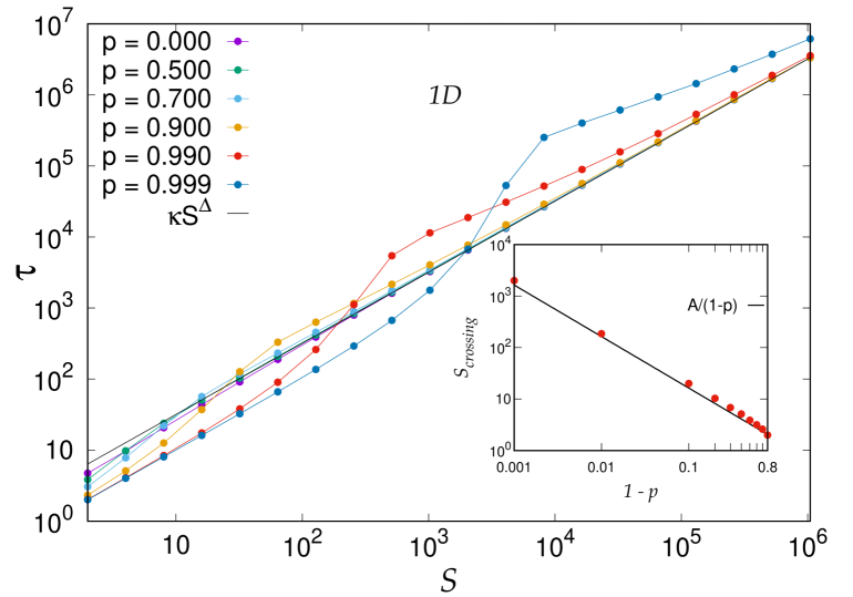
Figure 1: Lifetime $\tau$ against starvation time $S$ for $0\leqslant p<1$. Power law behavior is observed for $S\gg S_{crossing}$ as $\tau\sim\kappa S^{\Delta}$, with $\Delta\simeq 1$ and $\kappa\simeq 3.18$. In the inset, $S_{crossing}$ is plotted against $1-p$ and the curve is dictated by $S_{crossing}=\frac{A}{1-p}$, where $A=1.64\pm 0.03$.

From Fig. 1, it is clear that for any $0<p<1$, the curves start below the $p=0$ curve, cross the $p=0$ curve at some $S$ value, denoted as $S_{crossing}$, and then goes well above the $p=0$ curve. This ensures an increase in lifetime. For very high $S$ the curve asymptotically approaches the $p=0$ curve. The following points are also clear:

• For low $p$, the curves start (low $S$) just below $p=0$ curve. As $p$ is made higher, the starting point of the curves goes lower.

• $S_{crossing}$ is less (larger) for lower (higher) values of $p$. The variation of $S_{crossing}$ is shown in the inset of Fig. 1.

• For $S\gg S_{crossing}$ the behavior can be descrided as:

  $$\tau\propto S^{\Delta},$$ (6)

  with $\Delta\sim 1$.

The result for $p=0$, as shown in Fig. 1, clearly agrees with the result as mentioned in Redner2014 . For $p=1$, since the forager stays at the origin until starvation (no movement), it indicates $\tau=S$. Therefore, the result for $p=1$ (not shown as there is already a curve shown for $\tau=S$) and $p=0$ should be parallel in a log-log plot. For the intermediate values of $p$, a transition from $p=1$ line to $p=0$ line can be observed. In these cases, due to inertia, the forager partially retains its position and consumes less amount of food compared to $p=0$ case. For low $S$, which means the forager can survive for small time with one food morsel, if its position is restricted more with inertia, its lifetime becomes less. For very high $S$, however, it can live long once it gets food, and therefore even if its motion is somewhat restricted, it can survive longer. Increase in lifetime for higher $p$ for high $S$ indicates less consumption of food resulting in a smaller desert. For very high $S$, $\tau\sim S^{\Delta}$ with $\Delta\simeq 1$ independent of $p$.

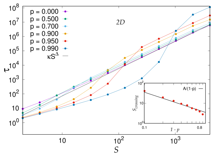
Figure 2: Lifetime $\tau$ against starvation time $S$ with $0\leqslant p<1$ in $2d$. Similar power law behavior as in Fig. 1 is observed with the exponent $\Delta\simeq 1.9$ and $\kappa\simeq 0.91$. $S_{crossing}$ against $1-p$ has been shown in inset and observed that $S_{crossing}=\frac{A}{1-p}$ where $A=3.52\pm 0.19$.

In the $2d$ case, the forager experiences greater freedom of movement, allowing it to explore more directions before encountering previously visited or depleted sites. This increased mobility leads to a higher value of the scaling exponent, with $\Delta\simeq 1.9$ as shown in Fig. 2 for high $S$. The overall behavior of the curves for different values of $p$ closely resembles the patterns observed in the one-dimensional case, indicating that the foraging dynamics remain qualitatively similar across dimensions.

The scaling behavior of $\tau$ for the forager in $2d$ with $p=0$, aligns with the findings as in Redner2014 .

The variation of $S_{croosing}$ for both $1d$ and $2d$ are found to be of the form :

$$S_{crossing}=\frac{A}{1-p}.$$ (7)

These variations are shown in the insets of Fig. 1 and 2 for $1d$ and $2d$ respectively. The values of $A$ are found to be approximately $1.64$ and $3.52$ respectively.

III.2 Average Number of Distinct Sites $N$

The average number of distinct sites, $N$ against $S$ with $p$ as a parameter in $1d$ and $2d$ is studied and are shown in Fig. 3 and Fig. 4 respectively.

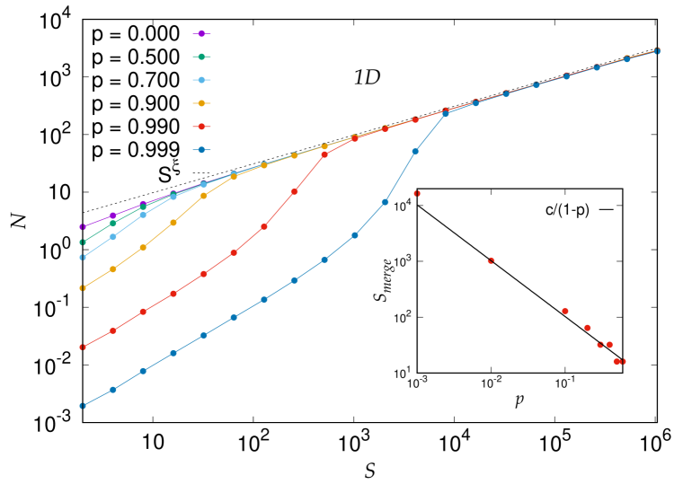
Figure 3: Behavior of average number of distinct site $N$ as a function of starvation time $S$ with $0\leqslant p<1$. For $S\gg S_{merge}$, power law behavior is observed, the exponent being $\xi=0.494\pm 0.002$. $S_{merge}$ against $p$ has been shown in the inset, which follows a relation $S_{merge}=\frac{c}{1-p}$ where, $c=10.26\pm 0.11$.

In the asymptotic limit, i.e. for large $S$, for any $p\neq 0$, it has been observed that, the average number of distinct sites $N$ shows power law behavior with $S$ and approaches the $p=0$ curve.

It is known that, for the unrestricted walker, the average number of distinct sites visited $N\simeq\sqrt{8S/\pi}$ Weiss . In Redner2014 , it was shown that $N$ goes as $\sqrt{S}$. Our results for $p=0$, both numerical and analytical, matches with Redner2014 . In general,

$$N\propto S^{\xi}$$ (8)

where, $\xi=0.494\pm 0.002$ in $1d$. At small $S$ region, as $p\rightarrow 1$, the curve shows linearity in the log-log plot. In the intermediate region, it shows some non-linearity and finally merges with $S^{\xi}$ at $S=S_{merge}$. In the inset of Fig. 3, we have shown the variation of $S_{merge}$ with $1-p$, and found that $S_{merge}$ follows the relation,

$$S_{merge}=\frac{c}{1-p}$$ (9)

where $c=10.26\pm 0.11$ in Fig. 3. Increase of $S_{merge}$ with $p$ is also due to more restriction for higher $p$.

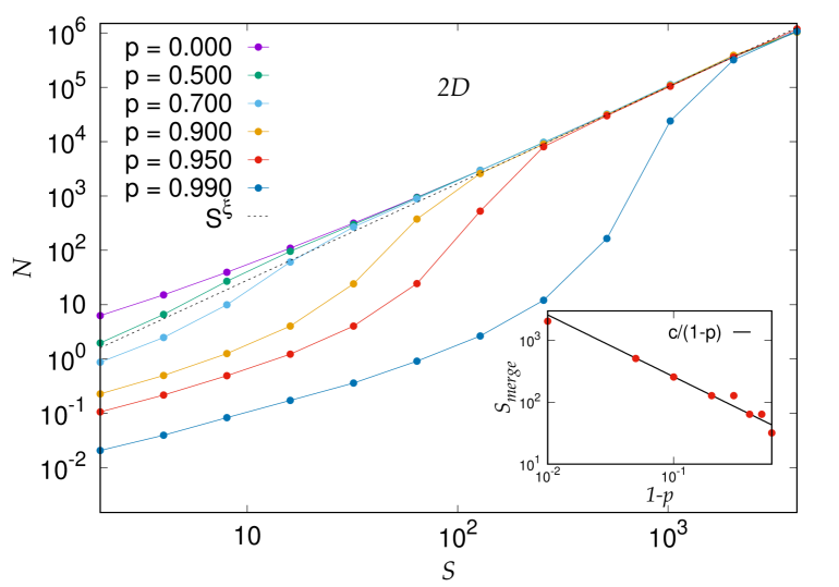
Figure 4: Average number of distinct site $N$ against starvation time $S$ in $2d$ with $0\leqslant p<1$. For $S\gg S_{merge}$, $\xi\simeq 1.78$. $S_{merge}=\frac{c}{1-p}$ is shown in the inset with $c=25.91\pm 0.84$.

In $2d$ case, forager has more freedom to access the food morsels, causing increment of average number of distinct sites. Here $\xi\simeq 1.78$, which matches quite well with Redner2014 . For $S_{merge}$, $c=25.91\pm 0.84$.

It is to be noted that the $p=1$ case is trivial because the forager stays at the origin until it starves to death i.e $N=1$, therefore we have not shown it in Fig. 3 and Fig. 4.

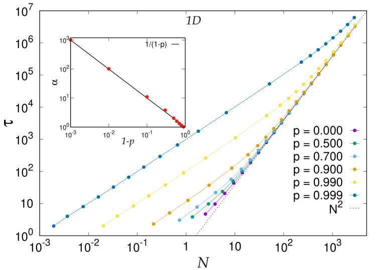
Figure 5: Variation of lifetime $\tau$ with average number of distinct site $N$ for $1d$. The variation follows the relation $\tau(N)=\alpha(p)N$ in small $N$ region for $p<1$. In the large $N$ region, the curve goes as $N^{2}$. In the inset, the variation of $\alpha$ with $1-p$ is shown as $\alpha=\frac{1}{1-p}$.

III.3 Relation between $\tau$ and $N$

Now, we would like to see the relation between $\tau$ and $N$. In $1d$ case, we used a heuristic approach in large $S$ region. Combining Eq. 6 and Eq. 8 we get $\tau\propto N^{2}$, which agrees with Fig. 5. For low values of $p$, from the Fig. 1 and 3 the behavior of $\tau\sim N$ which can be seen here too. For any $p<1$, there is a crossover behavior of the curves from $N$ to $N^{2}$ as $N$ is increased. That particular $N$ is shown as $N^{*}$ in Table 1. In the same table, the third column shows the $N$ values corresponding to $S_{merge}$ as found from Fig. 3. The lower $N$ region of the curves are fitted with,

$$\tau(N)=\alpha(p)N$$ (10)

$p$	$N^{*}$	$N$ at $S_{merge}$
$0.500$	$8$	$9$
$0.700$	$12$	$13$
$0.800$	$16$	$20$
$0.900$	$31$	$29$
$0.990$	$233$	$85$
$0.999$	$1195$	$230$

Table 1: Scaling behavior of number of distinct site at $S_{merge}$: $N^{*}\propto\frac{1}{(1-p)^{0.72}}$.

The variations of $\alpha(p)$ is shown in the inset of Fig. 5, where $\alpha$ follows the relation $\alpha(p)=\frac{1}{1-p}$.

III.4 Distribution of Distinct site $P(N)$

We study the distribution of average number of distinct sites $N$, denoted as $P(N)$. In $1d$ case, we run $10^{6}$ realizations and have shown distribution of $N$ in Fig. 6 with $p=0.000,0.500,0.990$ and $0.999$ and $S=2^{1}$ to $2^{13}$. For $p=0.000$ (a), the curves shows a dome like structure where the peak position moves with $\sqrt{S}$ in $1d$ which nicely agrees with the Fig. 3. The similar pattern also appears in $p=0.500$ case (b).

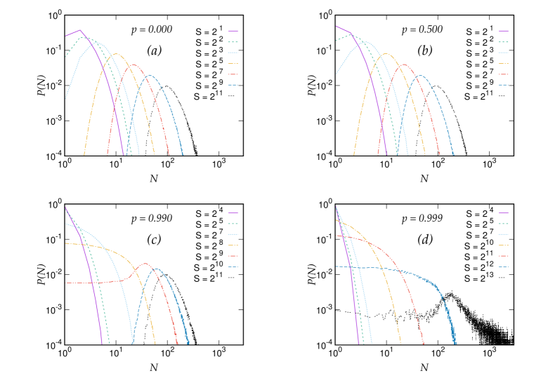
Figure 6: Distribution $P(N)$ of number of distinct site $N$ for (a) $p=0.000$, (b) $p=0.500$, (c) $p=0.990$ and (d) $p=0.999$.

Now, as we increase $p$, $S_{merge}$ plays some interesting role. For $p=0.990$ and $S<S_{merge}$ the dome shape has been lost ( Fig. 6(c)). It only appears when $S\geqslant S_{marge}$ and after that the dome shape continues. For $p=0.999$, the dome is only visible in $S\geqslant S_{merge}$ where $S_{merge}$ is as large as $2^{13}$ Fig. 6(d).

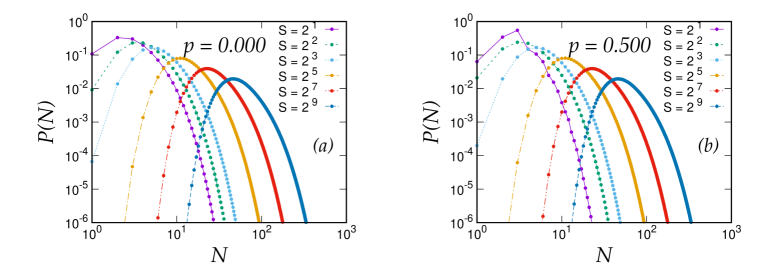
Figure 7: Distribution $P(N)$ of number of distinct site $N$ from analytical approach for (a) $p=0.000$, (b) $p=0.500$.

The distribution has been studied analytically starting from a diffusion equation which is shown in the Annexure in Eq. 14. The corresponding distribution function is shown in Eq. 3. The analytical result matches exactly with the result of the paper Redner2014 by putting $p=0$. However, for $p\neq 0$, the analytical result and numerical results do not match beyond $p=0.5$. for our case, the result matches up to $p=0.5$ quite well but not beyond. We have shown the analytical result for $p=0$ and $p=0.5$ in Fig. 7 (a) and (b) respectively. This may be due to the fact that the analytical result contains several factors that have to be approximated. There are certain integrations whose values are obtained numerically with certain approximations.

III.5 Distribution of Relaxation time $T(x)$

Since we are dealing with inertia, it is important to study the relaxation time also. Whenever the forager hits a food (say at $x$) it may rest (relax) for some time $T$, we denote the relaxation time at $x$ as $T(x)$. The detailed analysis of $T(x)$ will be discussed in this section.

The plot of average relaxation time $T(x)$ versus $x$ shows a maximum at the origin. Due to the initial condition the forager always has a finite probability to take rest at origin irrespective of $p$. It has been observed in Fig. 8 (shown in the inset) that the relaxation time follows the relation,

$$T(x)\propto\exp(-\kappa_{T}|x|)$$ (11)

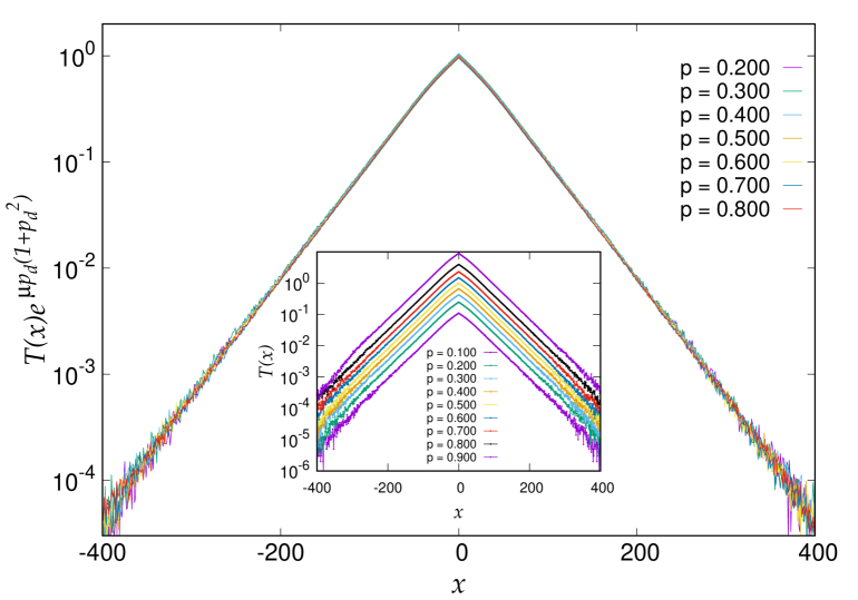
Figure 8: Behavior of relaxation time $T(x)$ over sites $x$. Data collapse of $T(x)e^{\mu p_{d}(1+p_{d}^{2})}$ against $x$ has been shown with $0.20\leqslant p\leqslant 0.80$ with $\mu=4.3$ and $p_{d}=0.5-p$. In the inset plot of relaxation time $T(x)$ against sites $x$ has shown.

The curves show symmetry and as $p$ increases, $T(x)$ also increases. The data collapse for the same has also been shown in Fig. 8.

We denote the distribution of $T$ as $f(T)$. We have calculated $f(T)$ for $S=1024$ in $1d$ as well as in $2d$. In $1d$, the behavior is shown in Fig. 9.

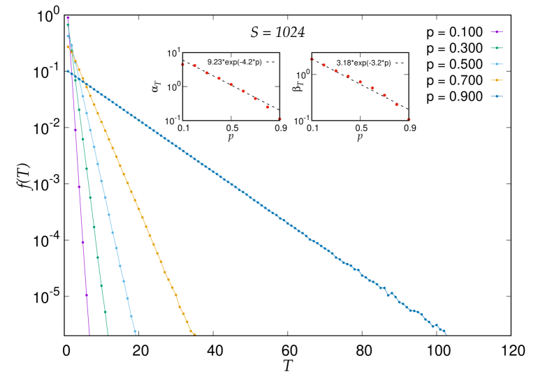
Figure 9: Distribution of Relaxation Time in $1d$ $f(T)$ against $T$ with $0.1\leqslant p\leqslant 0.9$ and $S=1024$. In the inset the variation of $\alpha_{T}(p)$ and $\beta_{T}(p)$ has shown.

It appears that the curve follows the relation,

$$f(T)=\alpha_{T}(p)\exp(-\beta_{T}(p)T)$$ (12)

Where $\alpha_{T}(p)$ and $\beta_{T}(p)$ also decay exponentially. The variation of $\alpha_{T}(p)$ and $\beta_{T}(p)$ are shown in the inset of Fig. 9. It has been found in $1d$ that $\alpha_{T}(p)=9.23\exp(-4.2p)$ and $\beta_{T}(p)=3.18\exp(-3.2p)$, whereas for $2d$ case, $\alpha_{T}(p)=11.2\exp(-4.5p)$ and $\beta_{T}(p)=3.12\exp(-3.1p)$.

III.6 Distribution of Inter-Encounter Time $P_{t}$

We define $N_{t}$ as the time interval between two successive food encounters by the forager. At each encounter with food, the forager’s internal energy resets to full, and the time until the next encounter is measured anew. Such intervals, collected until starvation, yields the distribution $P_{t}$.

The statistical properties of $P_{t}$ provide a detailed characterization of the foraging dynamics, reflecting the interplay between the forager’s motion, environmental structure, and food availability.

It is clear that $P_{t}$ depends on $N_{t}$ only, for any $p$. For small $p$, the dependence is $N_{t}^{-1.5}$ over almost the entire region and for larger $p$, only for large $N_{t}$. This should be related to the time interval between visiting two sites, both for the first time, for a diffusing walker as follows: It is well known that the First passage probability $F(t)\propto 1/t^{3/2}$ for a diffusing walker at large time $t$ RednerFP ; Basu Consider $t_{1}$ and $t_{2}$ be the times when visits are made for the first time and in between these two, all visits are not first time visits. We have $t_{2}-t_{1}=N_{t}$. Thus we have,

$$P_{t}=F(t_{1})\bigg{[}\prod_{i=1}^{t-1}(1-F(t_{1}+i))\bigg{]}F(t_{1}+N_{t}),$$ (13)

which can be calculated easily as the product term approaches $1$ for large time and therefore the dependence is $N_{t}^{-3/2}$ from the last term. This approach is of course correct when most of the time the forager performs usual random walk without resting, so matches the result for $p$ up to $\approx 0.5$ and also for larger values of $N_{t}$ when sites with food become rare and the forager is forced not to take rest most of the time. Beyond this value, the resting constributes in the dynamics, again for smaller values of $N_{t}$ only, when more sites with food are vailable. As a result a shallow peak occurs for larger values of $p$ at an intermediate value of $N_{t}$. The distributions are shown in Fig. 10.

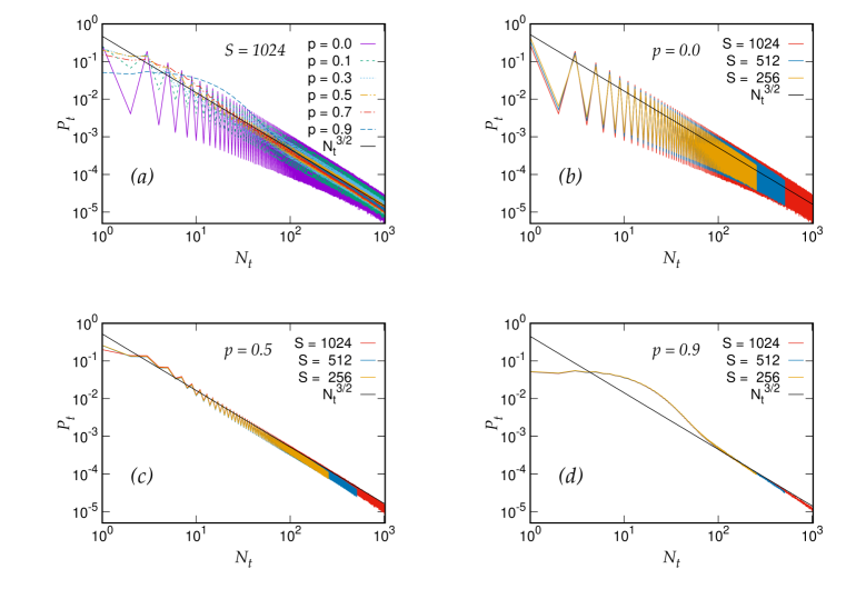
Figure 10: Plot of distribution $P_{t}$ of inter-encounter time $N_{t}$: (a) Varying $p$ with $S=1024$; (b) Varying $S$ for $p=0$; (c) Varying $S$ for $p=0.5$; and (d) Varying $S$ for $p=0.9$. For panels (b), (c), and (d), $S=256,512,1024$.

IV Conclusion

In this work, we studied a forager model on a $d$-dimensional lattice with starvation constraints and introduced a novel element of inertia, where the forager may rest with probability $p$ upon encountering food. The food is distributed uniformly on the lattice, and the forager can survive for $S$ steps without consuming any food further. We analyzed the system’s behavior by focusing on the key observables as follows: the average lifetime $\tau$ , the average number of distinct sites visited $N$ and the relaxation time $T(x)$ associated with a site $x$. Our results reveal rich dynamical features that strongly depend on both the starvation time $S$ and the inertia parameter $p$. For $p=0$, our studies for $\tau$ and $N$ align quite well with existing studies, For $p=0$, the known results have been reproduced both in one and two dimensions. The case $p=1$ yields trivial behavior, corresponding to a stationary forager with minimal survival. However, for intermediate values $0<p<1$, the system exhibits non-linear crossovers and new scaling regimes. Specifically, we identify two characteristic scales for $\tau$ and $N$ respectively as $S_{crossing}$ and $S_{merge}$ both proportional to $1/(1-p)$, beyond which the forager’s behavior aligns with the $p=0$ regime. These indicates that there is a strong influence of inertia on exploration dynamics. We further established a scaling relation between lifetime and distinct sites. A change in the scaling behavior has been observed below and above a particular $N$ value, viz., $N^{*}$; below $N^{*}$, $\tau\sim N$ and above $N^{*}$, $\tau\sim N^{2}$. The values $N^{*}$ for different $p$ are compared to the values of $N$ at $S_{merge}$ in Table 1 and they are quite similar. Thus, $\tau(N)=\alpha(p)N^{z}$, with $z=1$ or $2$ as mentioned, and $\alpha(p)=1/(1-p)$.

The relaxation time $T(x)$ was found to decay exponentially in space. The distribution of $T$, i.e., $P(T)$ follows an exponential form, with parameters dependent on $p$. The data collapse is shown in Fig. 8. Additionally, we studied the distribution of inter-encounter times, which further substantiates the model’s stochastic character.

All the results show that significant changes occur when $p>0.5$ where the results clearly deviate from those at $p=0$, at lease when $S$ is finite. This suggests that there is a threshold value of $p$ above which the effect of the inertia becomes non trivial. However, it is difficult to exactly detect the threshold value.

Altogether, this study demonstrates that the inclusion of inertia, an elementary yet biologically motivated modification, introduces significant changes to the statistical features of classical starving random walk models. These findings may be useful in understanding real-world foraging behavior, intermittent search processes, and transport phenomena in disordered systems.

In future, incorporating memory or adaptive strategies may enrich the model further, offering connections to a more realistic situation.

AM acknowledges financial support from CSIR, India (Grant no. 08/0463(12870)/2021-EMR-I). AM and SG acknowledges the computational facility of Vidyasagar College, University of Calcutta. PS acknowledges financial support from CSIR scheme 03/1495/23/EMR-II.

Appendix

The diffusion equation is modified with the introduction of the parameter $p$:

$$\frac{\partial u(x,t)}{\partial t}=\left(1-p\left(1-\braket{\frac{\eta_{t}}{\eta}}\right)\right)D\frac{\partial^{2}u(x,t)}{\partial x^{2}}$$ (14)

$$\frac{\partial u(x,t)}{\partial t}=\left(1-p\left(1-\left(\frac{t}{t+1}\right)^{\alpha}\right)\right)D\frac{\partial^{2}u(x,t)}{\partial x^{2}}$$ (15)

where, $\braket{\frac{\eta_{t}}{\eta}}=\left(\frac{t}{t+1}\right)^{\alpha}$ and $\braket{\eta}=N$, $\alpha=\alpha(p)$ it is found that $\alpha(0)=\frac{1}{2}$ and $\lim_{p\rightarrow 1}\alpha(p)=1$.
$\eta_{t}$ is the number visited site at time $t$ and $\eta$ is the number of visited site after starvation.
Using the method of separation of variable, we get,

$$u(x,t)=X(x)T(t)$$

$$\frac{1}{\left(1-p\left(1-\left(\frac{t}{t+1}\right)^{\alpha}\right)\right)D}\frac{1}{T}\frac{dT(t)}{dt}=\frac{1}{X}\frac{d^{2}X}{dx^{2}}=-\frac{\lambda^{2}}{a^{2}}$$ (16)

$$u(x,t)=\sum_{n=1}^{\infty}\left[A_{n}\sin\left(\frac{n\pi x}{ja}\right)+B_{n}\cos\left(\frac{n\pi x}{ja}\right)\right]\cdot\exp\left[-\left(\left(\frac{n\pi}{ja}\right)^{2}D\right)\int\left((1-p)+p\left(\frac{t}{t+1}\right)^{\alpha}\right)dt\right]$$ (17)

Assuming $t\gg 1$,

$$u(x,t)=\sum_{n=1}^{\infty}\left[A_{n}\sin\left(\frac{n\pi x}{ja}\right)+B_{n}\cos\left(\frac{n\pi x}{ja}\right)\right]\cdot\left[t^{\left(\frac{n\pi}{ja}\right)^{2}Dp\alpha}\exp\left(-\left(\frac{n\pi}{ja}\right)^{2}Dt\right)\right]$$ (18)

Boundary conditions are,

$$u(0,t)=u(ja,t)=0$$

(since the walker stops it $ja$)
We get $B_{n}=0$,

$$u(x,t)=\sum_{n=1}^{\infty}A_{n}\sin\left(\frac{n\pi x}{ja}\right)\left[t^{\left(\frac{n\pi}{ja}\right)^{2}Dp\alpha}\exp\left(-\left(\frac{n\pi}{ja}\right)^{2}Dt\right)\right]$$ (19)

To find the value of $A_{n}$ we will use fourier trick and the initial condition $u(x,0)=\delta(x-a)$ (since it starts from a distance $a$)

$$u(x,0) = \delta(x-a)$$

$$\sum A_{n}\sin\left(\frac{n\pi x}{ja}\right) = \delta(x-a)$$

$$\sum\int_{0}^{ja}A_{n}\sin^{2}\left(\frac{n\pi x}{ja}\right)dx = \int_{0}^{ja}\delta(x-a)\sin\left(\frac{n\pi x}{ja}\right)dx$$

$$A_{n} = \frac{2}{ja}\sin\left(\frac{n\pi}{j}\right)$$ (20)

Therefore,

$$u(x,t)=\frac{2}{ja}\sum_{n=1}^{\infty}\sin\left(\frac{n\pi}{j}\right)\sin\left(\frac{n\pi x}{ja}\right)\left[t^{\left(\frac{n\pi}{ja}\right)^{2}Dp\alpha}\exp\left(-\left(\frac{n\pi}{ja}\right)^{2}Dt\right)\right]$$ (21)

Instead of performing the integral, we calculate the flux across the boundary $[0,ja]$.

$$F_{j}(t) =D\left(\frac{\partial u}{\partial x}\bigg{|}_{x=0}-\frac{\partial u}{\partial x}\bigg{|}_{x=ja}\right)$$

$$=\frac{2D}{ja}\sum_{n=1}^{\infty}\frac{n\pi}{ja}\sin\left(\frac{n\pi}{j}\right)\left(1-(-1)^{n}\right)\left[t^{\left(\frac{n\pi}{ja}\right)^{2}Dp\alpha}\exp\left(-\left(\frac{n\pi}{ja}\right)^{2}Dt\right)\right]$$

$$=\frac{4\pi D}{(ja)^{2}}\sum_{n=1}^{\infty}(2n+1)\sin{\left(\frac{(2n+1)\pi}{j}\right)}\left[t^{\left(\frac{(2n+1)\pi}{ja}\right)^{2}Dp\alpha}\exp\left(-\left(\frac{(2n+1)\pi}{ja}\right)^{2}Dt\right)\right]$$

Now, $Q_{j}=\int_{0}^{S}F_{j}(t)dt$.
Assuming total flux that can escape is normalized to 1, we may write, $\lim_{S\rightarrow\infty}Q_{j}=1$.

Therefore,

$$Q_{j} =1-\int_{S}^{\infty}F_{j}(t)dt$$

$$=1-\frac{4\pi D}{(ja)^{2}}\sum_{n=1}^{\infty}(2n+1)\sin{\left(\frac{(2n+1)\pi}{j}\right)}\int_{S}^{\infty}\left[t^{\left(\frac{(2n+1)\pi}{ja}\right)^{2}Dp\alpha}\exp\left(-\left(\frac{(2n+1)\pi}{ja}\right)^{2}Dt\right)\right]$$

$$=1-\frac{4\pi D}{(ja)^{2}}\sum_{n=1}^{\infty}(2n+1)\sin{\left(\frac{(2n+1)\pi}{j}\right)}\frac{\gamma\left[\left(\frac{(2n+1)\pi}{ja}\right)^{2}Dp\alpha+1,\left(\frac{(2n+1)\pi}{ja}\right)^{2}DS\right]}{\left[\left(\frac{(2n+1)\pi}{ja}\right)^{2}D\right]^{\left(\frac{(2n+1)\pi}{ja}\right)^{2}Dp\alpha+1}}$$

$$Q_{j} =1-\frac{4}{\pi}\sum_{n=1}^{\infty}\frac{\sin{\left(\frac{(2n+1)\pi}{j}\right)}}{(2n+1)}\frac{\gamma\left[\left(\frac{(2n+1)\pi}{ja}\right)^{2}Dp\alpha+1,\left(\frac{(2n+1)\pi}{ja}\right)^{2}DS\right]}{\left[\left(\frac{(2n+1)\pi}{ja}\right)^{2}D\right]^{\left(\frac{(2n+1)\pi}{ja}\right)^{2}Dp\alpha}}$$ (22)

where, $\gamma(s,x)=\int_{0}^{x}t^{s-1}e^{-t}dt$
The probability distribution of number of distinct visited site $N$, i.e., $P(N)$,

$$P(N)=Q_{2}Q_{3}...Q_{N}(1-Q_{N+1}),$$ (23)

where $(1-Q_{N+1})$ signifies the exemption of $(N+1)^{th}$ site.
To calculate the explicit result we need to calculate the product of $Q_{j}$’s,

$$U_{N} =\prod_{2\leqslant j\leqslant N}Q_{j}$$

$$\log{U_{N}} =\sum_{j=2}^{N}\log{\left[1-\frac{4}{\pi}\sum_{n=1}^{\infty}\frac{\sin{\left(\frac{(2n+1)\pi}{j}\right)}}{(2n+1)}\frac{\gamma\left[\left(\frac{(2n+1)\pi}{ja}\right)^{2}Dp\alpha+1,\left(\frac{(2n+1)\pi}{ja}\right)^{2}DS\right]}{\left[\left(\frac{(2n+1)\pi}{ja}\right)^{2}D\right]^{\left(\frac{(2n+1)\pi}{ja}\right)^{2}Dp\alpha}}\right]}$$ (24)

Again from Eq. 22, for $j=N+1$,

$$1-Q_{N+1}=\frac{4}{\pi}\sum_{n=1}^{\infty}\frac{\sin{\left(\frac{(2n+1)\pi}{N+1}\right)}}{(2n+1)}\frac{\gamma\left[\left(\frac{(2n+1)\pi}{(N+1)a}\right)^{2}Dp\alpha+1,\left(\frac{(2n+1)\pi}{(N+1)a}\right)^{2}DS\right]}{\left[\left(\frac{(2n+1)\pi}{(N+1)a}\right)^{2}D\right]^{\left(\frac{(2n+1)\pi}{(N+1)a}\right)^{2}Dp\alpha}}$$ (25)

Now substituting Eq. 24 and 25 in Eq. 23 we get a general form of $P(N)$.

$$P(N)=\frac{4}{\pi}\sum_{m=1}^{\infty}\frac{\sin{\left(\frac{(2m+1)\pi}{N+1}\right)}}{(2m+1)}\frac{\gamma\left[\left(\frac{(2m+1)\pi}{(N+1)a}\right)^{2}Dp\alpha+1,\left(\frac{(2m+1)\pi}{(N+1)a}\right)^{2}DS\right]}{\left[\left(\frac{(2m+1)\pi}{(N+1)a}\right)^{2}D\right]^{\left(\frac{(2m+1)\pi}{(N+1)a}\right)^{2}Dp\alpha}}\\ \times\exp{\left[\sum_{2\leqslant j\leqslant N}\log{\left[1-\frac{4}{\pi}\sum_{n=1}^{\infty}\frac{\sin{\left(\frac{(2n+1)\pi}{j}\right)}}{(2n+1)}\frac{\gamma\left[\left(\frac{(2n+1)\pi}{ja}\right)^{2}Dp\alpha+1,\left(\frac{(2n+1)\pi}{ja}\right)^{2}DS\right]}{\left[\left(\frac{(2n+1)\pi}{ja}\right)^{2}D\right]^{\left(\frac{(2n+1)\pi}{ja}\right)^{2}Dp\alpha}}\right]}\right]}$$ (26)

Analytically dealing the incomplete gamma function in Eq. 26 is difficult, we calculated it numerically and for smaller value of $p$ Eq. 26 satisfy the simulation results in Fig. 6.

Setting $p=0$ in Eq. 26 we get,

$$P(N)\simeq\frac{4}{N}\sum_{m=1}^{\infty}\exp{\left[-\frac{(2m+1)^{2}\pi^{2}DS}{N^{2}a^{2}}-2\sum_{n=1}^{\infty}E_{1}\left(\frac{(2n+1)^{2}\pi^{2}DS}{N^{2}a^{2}}\right)\right]}$$ (27)

where, $E_{1}(x)=\int_{1}^{\infty}dt\frac{e^{-xt}}{t}$.

Eq. 27 exactly matches with the result of Redner2014 .

References

- (1) O. Stephen, Philosophical Transactions of the Royal Society B, 367, 770–784 (2012).
- (2) H. Robbins, American Mathematical Society Bulletin 58, 527 (1952).
- (3) J. C. Gittins, Journal of the Royal Statistical Society, Series B (Methodological) 41, 148 (1979).
- (4) M. A. Gottlieb, Feynmans Restaurant Problem Revealed.
- (5) T. T. Hills, M. N. Jones, and P. M. Todd, Psychological review 119, 431 (2012).
- (6) J. T. Abbott, J. L. Austerweil, and T. L. Griffiths, Psychol. Rev. 122(3), 558 (2015).
- (7) A. S. Chakrabarti, B. K. Chakrabarti, A. Chatterjee and M. Mitra, Physica A 388, Issue 12, 2420-2426 (2009).
- (8) O. Benichou, S. Redner, Phys. Rev. Lett. 113, 238101 (2014).
- (9) O. Bénichou, U. Bhat, P. L. Krapivsky, S. Redner, Phys. Rev. E 97, 022110 (2018).
- (10) M. Perman, W. Werner, Probab. Theory Relat. Fields 108 357 (1997).
- (11) I. Benjamini, D. B. Wilson, Electron. Commun. Probab. 8 86 (2003).
- (12) T. Antal, S. Redner, J. Phys. A 38 2555 (2005).
- (13) U. Bhat, S. Redner, J. Stat. Mech. 2022, 033402 (2022).
- (14) U. Bhat, S. Redner, O. Bénichou, J. Stat. Mech. 2017, 073213 (2017).
- (15) O. Bénichou, M. Chupeau, S. Redner, J. Phys. A: Math. Theor. 49, 394003 (2016).
- (16) G. H. Weiss, “Aspects and Application of the Random Walk”, (North-Holland, Amsterdam, 1994).
- (17) S. Redner, ”A Guide to First-Passage Processes” (Cambridge University Press, New York, 2001).
- (18) A. K. Basu, M. T. Wasan, Scandinavian Actuarial Journal, 1975(2) 99–108 (1975).