Cluster sizes, particle displacements and currents in transport
mediated by solitary cluster waves

Abstract

In overdamped particle motion across periodic landscapes, solitary cluster waves can occur at high particle densities and lead to particle transport even in the absence of thermal noise. Here we show that for driven motion under a constant drag, the sum of all particle displacements per soliton equals one wavelength of the periodic potential. This unit displacement law is used to determine particle currents mediated by the solitons. We furthermore derive properties of clusters involved in the wave propagation as well as relations between cluster sizes and soliton numbers.

I Introduction

Collective transport of particles in crowded systems frequently involves coherent motion of particle assemblies. Important examples are driven dynamics in biological pores and synthetic channels [1, 2, 3], intracellular particle transport [4], crowdion-mediated atomic diffusion on solid surfaces [5], and driven motions of micron-sized particles in colloidal suspensions [6, 7, 8, 8, 9, 10, 11, 12, 13, 14, 15, 16].

A minimal model for studying such cluster-mediated collective dynamics is that of hardcore interacting particles performing overdamped Brownian in periodic potentials [17, 18]. This model has been termed Brownian asymmetric simple exclusion process (BASEP) [19] since it resembles the prominent asymmetric simple exclusion process, a fundamental model in nonequilibrium statistical mechanics [20, 21, 22, 23].

Recently, solitary cluster waves were theoretically predicted [24] to occur in the one-dimensional BASEP and experimentally confirmed for driven Brownian motion of microparticles across a periodic potential [25]. The solitary cluster waves emerge at high particle densities, when the filling of potential wells exceeds a certain limit. There exists a maximal filling, where the particles arrange into mechanically stable configurations in the periodic landscape under a constant drag force. The ensemble of these configurations defines the presoliton state. For higher fillings, running states are formed with particle transport mediated by cluster waves. The waves propagate by attachment and detachment events, where one cluster gets in contact with or looses contact from another cluster.

Solitary cluster wave dynamics can be synchronized with an external oscillatory driving [26], leading to phase-locked values of soliton-mediated particle currents and Shapiro steps in the change of currents upon modifying the period-averaged driving force. When analyzing properties of the phase-locked currents, a unit displacement law (UDL) was conjectured, saying that the sum of all particle displacements during one period of soliton motion is equal to the wavelength of the period potential.

Here we prove the UDL for the sinusoidal potential and weak constant drag force. The proof suggests that the UDL is valid also for large drag forces and arbitrary periodic potentials and we test this by numerical simulations. Based on the UDL we derive cluster sizes involved in the soliton propagation, relations to the number of solitons occurring in the system, and particle currents mediated by solitary cluster waves.

Considering the complexity of presoliton states, the UDL is surprising. In a presoliton state, particles can arrange into different configurations, where in each configuration a different set of cluster sizes is present. By contrast, particle configurations are made of same cluster types in a running state. This aspect of heterogeneity of presoliton states and homogeneity of soliton-carrying states was not addressed in the previous work [27]. We discuss it in this study and show that the heterogeneity in presoliton states is decreasing with driving force and system size. In the thermodynamic limit, only the number of the largest stabilizable clusters is extensive.

The UDL is remarkable also in view of the fact that individual particle displacements in one soliton period are different.

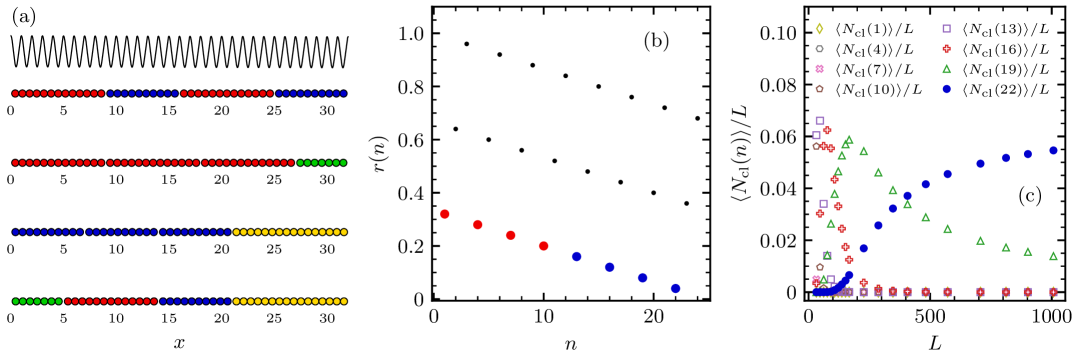
Figure 1: Particle clusters in the presoliton state for particle diameter $\sigma=0.68$ and drag force $f=10^{-3}$, representing the regime of infinitesimal $f$. (a) Examples of four simulated particle configurations in the presoliton state of a system with $L=32$ potential wells, obtained by evolving initial configurations with randomly chosen particle positions until a mechanically stable state is reached. In these configurations, stable clusters of sizes $n=7$ (green), 10 (blue), 13 (red), and 16 (yellow) appear. (b) Residual free space $r(n)$ [Eq. (5)] as a function of $n$. Bold circles give $r(n)$ of the possible mechanically stable $n$-clusters according to the free space theorem. These $n$-clusters are stable and can occur in configurations of the presoliton state for $f=0^{+}$. For finite $f=0.05$, the red circles correspond to possible mechanically stable $n$-clusters, while the blue ones to $n$-clusters that become unstable due to the larger $f$. (c) Mean cluster numbers $\langle N_{\rm cl}(n)\rangle/L$ per potential well as a function of $L$, showing that only $\langle N_{\rm cl}(n_{\rm b}=22)\rangle$ is extensive in system size. The averaging $\langle\ldots\rangle$ was performed over 500 initial particle configurations.

II Driven overdamped motion of hard spheres in periodic potentials

We consider $N$ hard spheres that are dragged by a constant force $f$ accross a one-dimensional periodic potential $U(x)$ with wavelength $\lambda$ in a fluidic environment. If the potential barriers are much larger than the thermal energy, thermal noise effects become negligible and equation of motions can be written as [27]

$$\frac{\differential x_{i}}{\differential t}=f-\frac{\differential U}{\differential x_{i}}\,,\hskip 10.00002pti=1,\ldots,N\,,$$ (1)

where $x_{i}$ are the particle positions. They satisfy the hard-sphere constraints

$$|x_{j}-x_{i}|\geq\sigma\,,$$ (2)

where $\sigma$ is the particle diameter. Equations (1) are given in dimensionless units. We have taken the wavelength $\lambda$ and barrier height $U_{0}$ of the periodic potential $U(x)$ as length and energy unit, and $\lambda^{2}/\mu U_{0}$ as the time unit, where $\mu$ is the particle mobility or inverse friction coefficient. The system size $L$ is an integer, $L\in\mathbb{N}$, and periodic boundary conditions are used.

For the sinusoidal potential,

$$U(x)=\frac{1}{2}\cos(2\pi x)\,.$$ (3)

As an example for a non-sinusoidal potential, we choose the smoothed triangle wave

$$U_{\delta}(x)=\frac{1}{2}\left(1-\frac{2}{\pi}\arccos[(1-\delta)\cos(2\pi x)]\right)\,,$$ (4)

where for $\delta>0$ the cusps of the triangles are rounded.

We consider particle diameters $\sigma<1$ in the following. Dynamics for larger particle diameters $\sigma+j$, $j\in\mathbb{N}$ can be mapped onto that for $\sigma\in[0,1)$, because the equations of motion (1) are invariant under a transformation $x_{i}\to x_{i}-j$; for details, see [17, 27].

To solve the equations of motions (1), we apply the Brownian cluster dynamics method [28].

III Heterogeneous presoliton and unique soliton-carrying states

In a recent study [27], a detailed theory was presented for soliton formation, propagation and soliton-mediated particle currents in the tilted sinusoidal potential. An essential concept in this theory is the presoliton state. It is the mechanically stable state with largest number of particles.

The presoliton state can be realized by different particle configurations. Examples are shown in Fig. 1(a) for the sinusoidal potential with $L=32$ wells, $N_{\rm pre}=45$ particles, and particle diameter $\sigma=0.68$. The drag force is $f=10^{-3}$, which represents the regime of infinitesimal drag force $f=0^{+}$. We generated the mechanically stable configurations by evolving randomly chosen initial particle positions. In each configuration, clusters appear, where $n$ particles are in contact. Specifically, we observe $n$-clusters with $n=7$, 10, 13, and 16 in the configurations in Fig. 1(a). Which cluster sizes occur is determined by the initial conditions.

Possible mechanically stable clusters in particle configurations of a presoliton state can be determined from a free space theorem [27]. It states:
    An $n$-cluster is stabilizable, if and only if its residual free space is smaller than that of $n^{\prime}$-clusters with $n^{\prime}<n$.

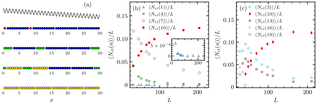
Figure 2: Particle clusters in the presoliton and soliton-carrying running states for the same particle diameter $\sigma=0.68$ as in Fig. 1 but for finite drag force $f=0.05$. (a) Examples of four simulated particle configurations in the presoliton state of a system with $L=32$ potential wells. Stable clusters of sizes $n=1$ (red), $n=4$ (green), 7 (yellow), and 10 (blue) appear. (b) Mean cluster numbers $\langle N_{\rm cl}(n)\rangle/L$ per potential well as a function of $L$. Only $\langle N_{\rm cl}(n)\rangle$ for $n=n_{\rm b}=10$ is extensive in system size. The inset shows a zoom-in of $\langle N_{\rm cl}(n)\rangle/L$ for $n=1$. (c) Same as (b) for the running state, showing that the non-propagating clusters (full symbols) all become $n_{\rm b}$-clusters for large $L$. Averaging $\langle\ldots\rangle$ in (b) and (c) was performed over 500 initial particle configurations.

The residual free space of an $n$-cluster is

$$r(n)=m(n)-n\sigma\,,$$ (5)

where

$$m(n)=\lceil n\sigma\rceil$$ (6)

equals the minimal number of potential wells needed for accommodating the $n$-cluster. Here, $\lceil\ldots\rceil$ is the Gaussian bracket for the ceiling function, i.e. $\lceil a\rceil$ is the smallest integer larger than $a$.

Figure 1(b) shows the residual free spaces $r(n)$ for $n$-clusters composed of particles of size $\sigma=17/25=0.68$. Applying the free space theorem, we conclude that only clusters with sizes $n=1$, 4, 7, 10, 13, 16, 19, and 22 can appear in particle configurations of the presoliton state. They are marked by red and blue circles in the figure. The clusters in Fig. 1(a) indeed all belong to the respective sequence of cluster sizes.

Inspite of the different clusters in the configurations of Fig. 1(a), each configuration has the same number $N_{\rm pre}=42$ of particles. In fact, $N_{\rm pre}$ is unique for a presoliton state and was derived for infinitesimal force $f=0^{+}$ and particle diameters $\sigma=\sigma_{p,q}=p/q$, where integers $p$ and $q$ are taken to be coprime and $p<q$ ($\sigma<1$). Only for these $\sigma_{p,q}$, running solitons can occur for $f=0^{+}$. It holds [27]

$$N_{\rm pre}=\left\lfloor\frac{L}{m_{\rm b}}\right\rfloor n_{\rm b}+\left\lfloor\frac{L\operatorname*{\,mod\,}m_{\rm b}}{\sigma}\right\rfloor\,,$$ (7)

where

$$n_{\rm b}=q\left\lceil\frac{p^{\varphi(q)-1}}{q}\right\rceil-p^{\varphi(q)-1}$$ (8)

is the largest mechanically stable cluster in the presoliton state, and

$$m_{\rm b}=m(n_{\rm b})=\lceil n_{\rm b}\sigma\rceil\,.$$ (9)

In Eq. (7), $\lfloor\ldots\rfloor$ denotes the floor function, i.e. $\lfloor a\rfloor$ is the largest integer smaller than $a$, and $a\operatorname*{\,mod\,}b=a-\lfloor a/b\rfloor b$ denotes the modulo operation. The function $\varphi(.)$ in Eq. (8) is Euler’s Phi (totient) function [29].

For the example in Fig. 1(a), $p=17$ and $q=25$, and $n_{\rm b}=22$ from Eq. (8). This is indeed the largest stabilizable cluster found in Fig. 1(b). For the system size $L=32$ in Fig. 1(a), we obtain $N_{\rm pre}=45$ from Eq. (7), in agreement with the particle number in the different configurations.

The derivation of Eq. (7) was done by considering a maximal homogeneous particle configuration of the presoliton state formed by a sequence of equally spaced largest stabilizable $n_{\rm b}$-clusters and by covering the rest part $L-\lfloor L/m_{\rm b}\rfloor m_{\rm b}$ of the system by smaller stabilizable clusters. In fact, the free space theorem tells us that the $n_{\rm b}$-cluster has smallest residual free space $r(n_{\rm b}$) among the stabilizable clusters and hence is most efficient when trying to cover the system with largest number of particles without loosing mechanically stability. Imagine, to the contrary, that $n_{\rm b}>1$ and one would start to fill a system with the smallest stabilizable clusters of size one, i.e. single particles. Then, after placing a finite number of single particles, it is possible to combine $n_{\rm b}$ of them and by this to generate enough additional free space to place a further particle without loosing mechanical stability.

Because of this, we expect that when increasing the system size $L$, only the most efficient covering by $n_{\rm b}$-clusters will prevail. As a consequence, the number of $n$-clusters appearing in configurations of the presoliton state should be extensive for $n=n_{\rm b}$ only. More precisely, if we take the set of all mechanically stable particle configurations of a presoliton state, each of these configurations has some number $N_{\rm cl}(n)$ of $n$-clusters. Averaging over all configurations yields the mean number $\langle N_{\rm cl}(n)\rangle$ of $n$-clusters in the presoliton state. The fraction $\langle N_{\rm cl}(n_{\rm b})\rangle/L$ then should approach a finite value when $L\to\infty$, while $\langle N_{\rm cl}(n)\rangle/L\to 0$ for $n<n_{\rm b}$. Results in Fig. 1(c) agree with this prediction.

Equations (7) and (8) were derived for infinitesimal drag force $f=0^{+}$. For finite $f>0$, one needs to take into account that for each cluster size $n$, there exists a critical force $f_{c}(\sigma,n)$. For $f>f_{c}(\sigma,n)$, an $n$-cluster looses mechanical stability. This effect reduces the size of the largest stabilizable cluster to a value $n_{\rm b}(f)\leq n_{\rm b}(f=0^{+})$, as illustrated by the blue and red circles in Fig. 1(b). Interestingly, simulation results suggest that the free space theorem still holds true, i.e. all stabilizable clusters can be inferred from it.

Let us demonstrate this for the same particle diameter $\sigma=0.68$ as considered in Fig. 1, choosing a drag force $f=0.05$, for which $n_{\rm b}=10$. Figure 2 shows results for this case. In the particle configurations of the presoliton state shown in Figure 2(a), stable clusters of sizes $1$, 4, 7, and 10 now appear. As the free space theorem still holds true, they are the same as identified from the minimal residual free spaces $r(n)$ of $n$-clusters in Fig. 1(b). However, we have to exclude all $n>10$, for which stability is lost due to the larger drag force. The stabilizable clusters for $f=0.05$ having sizes $n\leq n_{\rm b}(f)=10$ are marked in red in Fig. 1(b).

Figure 2(b) shows that mean cluster numbers in the presoliton behave analogously with increasing system size: $\langle N_{\rm cl}(n)\rangle/L\to 0$ for all $n<n_{\rm b}$ and $\langle N_{\rm cl}(n_{\rm b})\rangle/L\to 1/m_{\rm b}$. Remarkably, in the running state non-propagating clusters have the unique size $n_{\rm b}$, see the full symbols in Fig. 2(c). Other clusters (open symbols) are involved in the soliton propagation.

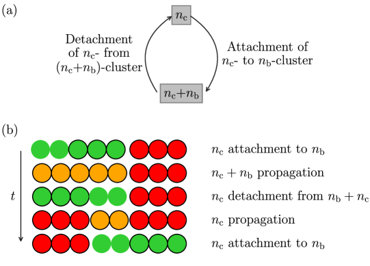
Figure 3: Illustration of a soliton propagation. (a) Soliton core cluster of size $n_{\rm c}$ and soliton composite cluster of size $n_{\rm b}+n_{\rm c}$ form in a periodic process of cluster attachments and detachments and give rise to a solitary cluster wave. (b) One period of soliton motion, where in the 1st row a core $n_{\rm c}$-cluster (green without circle boundaries) attaches to an $n_{\rm b}$-cluster (green), the formed composite $(n_{\rm c}\!+\!n_{\rm b})$-cluster (orange) thereafter moves in the 2nd row until a core $n_{\rm c}$-cluster detaches from its front in the 3rd row (green without circle boundaries). This $n_{\rm c}$-cluster (orange) moves in the 4th row until attaching to an $n_{\rm b}$-cluster in the 5th row, which completes the period.

As illustrated in Fig. 3(a), soliton propagates in a periodic process involving attachments and detachments of a core soliton $n_{\rm c}$-cluster to and from $n_{\rm b}$-clusters. In the sinusoidal potential, one soliton period can be described as follows, see Fig. 3(b). At the beginning of a period, a composite $(n_{\rm c}+n_{\rm b})$-cluster (green) is formed by attachment of an $n_{\rm c}$-cluster (green circles without black circle borders) to an $n_{\rm b}$-cluster (red). This composite cluster moves until it becomes unstable and an $n_{\rm c}$-cluster detaches from its front part. The detached $n_{\rm c}$-cluster (orange) thereafter moves until a new soliton period starts, when the $n_{\rm c}$-cluster attaches to the next $n_{\rm b}$-cluster .

In Fig. 3(c), $n_{\rm b}=10$ and $n_{\rm c}=3$, and accordingly the composite cluster has size $n_{\rm b}+n_{\rm c}=13$. Indeed, the only propagating clusters have size 3 and 13 at large $L$. Only for small $L$ of order $m_{\rm b}$, other propagating clusters may appear.

IV Unit displacement law

Particle displacements in states carrying $N_{\rm sol}$ solitary cluster waves are of different types. Particles forming core $n_{\rm c}$- and composite $(n_{\rm c}+n_{\rm b})$-clusters are translated by a soliton, while those forming $n_{\rm b}$-clusters relax towards position of mechanical equilibria. This relaxation is heterogeneous in space, because it depends on the distances from solitary waves. Inspite of this complexity, a remarkably simple unit displacement law holds:
  After one soliton period, the sum $\mathcal{D}$ of all particle displacements per soliton is equal to the wavelength of the potential:

$$\frac{\mathcal{D}}{N_{\rm sol}}=1\,.$$ (10)

We prove this law for a sinusoidal potential in the limit of infinitesimal drag force in Sec. IV.1. For finite drag forces and an example of a non-sinusoidal potential, we test its validity by simulations in Sec. IV.2.

IV.1 Proof of unit displacement law for sinusoidal potential and infinitesimal drag force

For a steady state carrying $N_{\rm sol}$ solitons, the sum of particle displacements in one soliton period can be calculated by considering two subsequent time instants, where an $n_{\rm c}$-cluster attaches to an $n_{\rm b}$-cluster. Two particle configurations at such instants are illustrated in Fig. 4. In the initial particle configuration in the upper row, we labeled the particles from 1 to $N$, starting with the particle right from the origin $x=0$. The particle positions in this configurations are $x_{i}$, $i=1,\ldots,N$, and in the final configuration after one soliton period (lower row) they are $x_{i}^{\prime}$. The sum of particle displacements is

$$\mathcal{D}=\sum_{i=1}^{N}(x_{i}^{\prime}-x_{i})\,.$$ (11)

The initial and final configurations are equivalent. For example, particles 1, 2, 3, 4 in the final configuration in Fig. 4 correspond to particles $N\!-\!1$, $N$, 1, 2 in the initial configuration. Hence, if we shift the particle indices of the final configuration by $-n_{\rm b}=-2$, we obtain the corresponding particle indices (modulo $N$) in the initial configuration. As a consequence of the equivalence, the particle positions are related as

$$x_{i}^{\prime}=\left\{\begin{array}[]{cc}x_{i-n_{\rm b}+N}+\lambda_{\rm sol}-L\,,&i=1,\ldots,n_{\rm b}\,,\\[4.30554pt] x_{i-n_{\rm b}}+\lambda_{\rm sol}\,,&i=n_{\rm b}+1,\ldots,N\,.\end{array}\right.$$ (12)

The periodic boundary conditions are taken into account by taking particle indices modulo $N$ and particle positions modulo $L$.

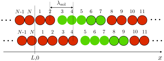
Figure 4: Upper row: particle configuration at a time instant, where an $n_{\rm c}$-cluster attaches to an $n_{\rm b}$-cluster ($n_{\rm c}=3$, $n_{\rm b}=2$). Basic $n_{\rm b}$-clusters are marked in red. The $(n_{\rm c}+n_{\rm b})$-cluster marked in green is forming in the attachment process. Lower row: Equivalent configuration after one soliton period, where particles with index $i$ correspond to particles with index $i-n_{\rm b}$ (modulo $N$) in the upper row. The distance between corresponding particles is equal to the soliton period $\lambda_{\rm sol}$, see Eq. (12). Particles of the attaching clusters in the two equivalent configurations are depicted without black circle borders. The vertical dashed line indicates the origin $x=0$ of the $x$-axis, which is identical to $x=L$ due to periodic boundary conditions.

Inserting Eq. (12) into Eq. (11), we obtain

$$\mathcal{D}=N\lambda_{\rm sol}-n_{\rm b}L\,,$$ (13)

i.e. $\mathcal{D}$ must be an integer.

We now show that $\mathcal{D}$ is an integer multiple of $N_{\rm sol}$ by taking into account two conditions: First, the total number of particles in $N_{\rm b}$ basic clusters composed of $n_{\rm b}$ particles and $N_{\rm sol}$ soliton clusters composed of $n_{\rm sol}=n_{\rm c}+n_{\rm b}$ particles must equal the particle number $N$,

$$N_{\rm b}n_{\rm b}+N_{\rm sol}n_{\rm sol}=N\,.$$ (14)

Second, in the running state, all potential wells must be occupied by clusters to enable soliton propagation by sequential attachments and detachments processes, see Fig. 3. Accordingly, the sum of potential wells occupied by the clusters gives the system size $L$,

$$N_{\rm b}m_{\rm b}+N_{\rm sol}m_{\rm sol}=L\,.$$ (15)

Here, $m_{\rm sol}$ is the number of potential wells needed for containing one soliton and $m_{\rm b}$ is given in Eq. (9).

For the sinusoidal potential, the distance $\lambda_{\rm sol}$ traveled by a soliton in one period is equal to $m_{\rm b}$ [27]. This can be intuitively understood from the soliton propagation discussed in Sec. III: after completing one soliton period, an $n_{\rm b}$-cluster is created that is accommodated by $m_{\rm b}$ wells – see the example in Fig. 4, where the 2-cluster composed of particles 3 and 4 in the lower row is created by the soliton movement. Associated with this process is a displacement of the two equivalent particle configurations by $\lambda_{\rm sol}$.

Taking $\lambda_{\rm sol}=m_{\rm b}$, and inserting $N$ and $L$ from Eqs. (14) and (15) into Eq. (13), we obtain

$$\mathcal{D}=N_{\rm sol}(n_{\rm sol}m_{\rm b}-n_{\rm b}m_{\rm sol})\,.$$ (16)

In the limit of infinitesimal drag force, where soliton propagation can occur only for certain rational particle sizes $\sigma_{p,q}=p/q$, $n_{\rm sol}=q$, $m_{\rm b}=\lceil n_{\rm b}\sigma_{p,q}\rceil=n_{\rm b}(p/q)+1/q$, and $m_{\rm sol}=\lceil n_{\rm sol}\sigma_{p,q}\rceil=p$ [27]. This implies

$$n_{\rm sol}m_{\rm b}-n_{\rm b}m_{\rm sol}=q\left(\frac{p}{q}\,n_{\rm b}+\frac{1}{q}\right)-n_{\rm b}p=1\,.$$ (17)

Hence, Eq. (10) holds for infinitesimal drag force.

IV.2 Tests of unit displacement law by simulations

For finite $f=0.2$ in the sinusoidal potential, simulation results for $n_{\rm b}$, $n_{\rm b}+n_{\rm c}$ and $N_{\rm sol}$ are shown for various $\sigma_{p,q}$ in Fig. 5(a). The system size is $L=30$ and particle numbers are $N=N_{\rm pre}+1$, i.e. we added one particle to the presoliton state. While $n_{\rm b}$ and $n_{\rm b}+n_{\rm c}$, and the number of solitons vary strongly with $\sigma$ and without obvious regularity, the sum of particle displacements per soliton $\mathcal{D}/N_{\rm sol}$ is always one, as shown in the inset of Fig. 5(a).

For the same system size $L=30$ and drag force $f=0.2$, we display in Fig. 5(b) corresponding simulation results for the triangle wave potential (4) with smoothing parameter $\delta=0.02$. The soliton propagation can be more complex in this potential, involving more cluster types. Instead of $n_{\rm b}+n_{\rm c}$, we show the size $n_{\rm max}$ of the largest cluster appearing in the soliton propagation. Analogous to the sinusoidal potential, $n_{\rm b}$, $n_{\rm max}$ and $N_{\rm sol}$ vary strongly and in an irregular manner with $\sigma$, whereas $\mathcal{D}/N_{\rm sol}=1$ in all cases.

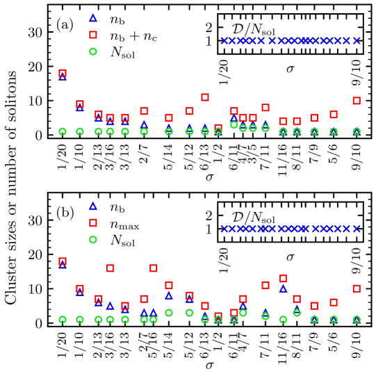
Figure 5: Verification of UDL by simulations. Sizes of largest ($n_{\rm b}+n_{\rm c}$ or $n_{\rm max}$) and basic stable clusters ($n_{\rm b}$) for different particle diameters $\sigma=p/q$, together with number $N_{\rm sol}$ of solitons. Part (a) shows the results for a sinusoidal potential and part (b) for the triangle wave potential (4) with smoothing parameter $\delta=0.02$. In both cases the system size is $L=30$ and the drag force $f=0.2$. Inspite of strong and irregular variation of the cluster sizes and number of solitons, the total sum $\mathcal{D}$ of particle displacements in one soliton period is equal to $N_{\rm sol}$, see insets.

We would like to point out that the individual particle displacements in one soliton period are different. If a single particle is part of a cluster relaxing towards a position of mechanical equilibrium, its displacement depends on how much the cluster is away from its point of stability. If a single particle is involved in the soliton propagation, its displacement depends on the soliton cluster of which it is part of and how much this cluster becomes displaced in one soliton period. Hence, there is a strong heterogeneity of individual particle displacements but irrespective of this feature, the sum of all particle displacements obeys the simple rule (10).

V Implications of UDL

The UDL allows us to determine the spatial extension $m_{\rm sol}$ of a soliton, and to derive particle currents mediated by solitary cluster waves. Furthermore, it determines $n_{\rm c}$ up to an integer multiple of $n_{\rm b}$. When adding a single particle to the system, it relates the increase $\delta N_{\rm sol}$ of soliton number and decrease $\-\delta N_{\rm b}$ of number of $n_{\rm b}$-clusters to $m_{\rm b}$ and $m_{\rm sol}$.

V.1 Spatial extension of solitons

For the soliton extension, we obtain from Eqs.  (10) and (16)

$$m_{\rm sol}=\frac{1}{n_{\rm b}}(n_{\rm sol}\,m_{\rm b}-1)\,.$$ (18)

In experiments, this expression can be evaluated by determining the size $n_{\rm b}$ of the relaxing basic cluster and the maximal number $n_{\rm sol}$ of particles involved in the soliton propagation.

It is important to note that $m_{\rm sol}$ is not equal to $\lceil n_{\rm sol}\sigma\rceil=\lceil(n_{\rm b}+n_{\rm c})\sigma\rceil$ in general. For example, in case of the sinusoidal potential and particle diameter $\sigma=0.61$, $n_{\rm b}=3$ and $n_{\rm c}=2$ for $f=0.3$. This yields the soliton extension $m_{\rm sol}=3$ according to Eq. (18), while the number of wells accommodating an $n_{\rm sol}$-cluster is $\lceil n_{\rm sol}\sigma\rceil=\lceil(n_{\rm b}+n_{\rm c})\sigma\rceil=4$.

V.2 Soliton-mediated particle currents

From the UDL follows a simple expression for the particle current $J$: the mean particle velocity is $\mathcal{D}/N\tau_{\rm sol}$, where $\tau_{\rm sol}$ is the time period of the solitary wave propagation, i.e. the time needed for the soliton to move a distance $\lambda_{\rm sol}=m_{\rm b}$. Multiplying this mean velocity with the number density $N/L$ yields

$$J=\frac{N}{L}\frac{\mathcal{D}}{N\tau_{\rm sol}}=\frac{N_{\rm sol}}{L\tau_{\rm sol}}\,.$$ (19)

For the sinusoidal potential, explicit expressions for $N_{\rm sol}$ and $\tau_{\rm sol}$ in terms of $\sigma$, $L$, $n_{\rm b}$, and $n_{\rm c}$ are given in [27].

Also, another derivation of the particle current was provided, yielding the seemingly unrelated result

$$J=\frac{N_{\rm sol}d}{n_{\rm b}L+N_{\rm sol}d}\frac{N}{L}\frac{m_{\rm b}}{\tau_{\rm sol}}\,,$$ (20)

where $d$ is the displacement of each particle after a single soliton has traveled a distance $n_{\rm b}L+d$ .

Comparing Eqs. (19) and (20) yields

$$n_{\rm b}+\frac{N_{\rm sol}}{L}d=\frac{N}{L}m_{\rm b}d\,.$$ (21)

The equation must hold true for all system sizes $L$. We thus can increase $L$ by adding $Mm_{\rm b}$ potential wells, where in each of the $M$ intervals $m_{\rm b}$ we place one basic stable $n_{\rm b}$-cluster. This way, we extend the system by only adding stable clusters, i.e. $N_{\rm sol}$ does not change. Accordingly, be letting $L\to L+Mm_{\rm b}$ and $N\to N+Mn_{\rm b}$ with $M\to\infty$, we obtain $N/L\to n_{\rm b}/m_{\rm b}$, $N_{\rm sol}/L\to 0$, and accordingly $n_{\rm b}=n_{\rm b}d$. Hence,

$$d=1\,.$$ (22)

This equation can be considered as an alternative statement of the UDL.

V.3 Changes of numbers of solitons and
basic stable clusters

Adding one particle to a running state, increases the number of solitons by $\delta N_{\rm sol}$ and decreases the number of stable clusters by $\delta N_{\rm b}$. It turns out that

$$\delta N_{\rm sol} =m_{\rm b}\,,$$ (23)

$$\delta N_{\rm b} =m_{\rm sol}\,.$$ (24)

Equation (23) follows by setting $d=1$ in Eq. (21) and calculating the change of $N_{\rm sol}$ when incrementing $N$ by one. The result for $\delta N_{\rm b}$ then follows from the space-filling condition (15) that implies $-\delta N_{\rm b}m_{\rm b}+\delta N_{\rm sol}m_{\rm sol}=0$, which, when using $\delta N_{\rm sol}=m_{\rm b}$, gives Eq. (24).

Based on Eq. (23) it is possible to design running states with controlled stepwise increase of solitons upon adding particles. A specific $m_{\rm b}=\delta N_{\rm sol}$ value can be realized by choosing $\sigma$ and $f$ to yield a corresponding size $n_{\rm b}$ of the basic stable cluster.

Equation (24) is useful to determine soliton sizes in experiments, where the detailed propagation process by cluster attachments and detachments can be difficult to resolve in view of the dense arrangement of the soliton clusters. By counting the number of clearly separated $n_{\rm b}$-clusters in running states, one can obtain $m_{\rm sol}=\delta N_{\rm b}$ in a feasible manner.

V.4 Soliton core cluster

While for the sinusoidal potential at finite $f>0$ it is possible to determine $n_{\rm b}$ quickly based on the cluster of maximal size with translational stability and by checking fragmentation stability for this and all clusters of smaller size, an efficient method for determining $n_{\rm c}$ is not yet available. For determining $n_{\rm c}$, we need to evaluate for increasing trial sizes $n_{\rm c}^{\prime}$ whether in two parts of a well defined interval of width $r(n_{\rm b})$, a core and composite soliton can propagate. This demanding procedure was discussed in Sec. 6 of Ref. [27]. We here show that the trial sizes of the core soliton cluster can be restricted to numbers incremented by $n_{\rm b}$.

When increasing $N$ by one, Eq. (14) implies $-n_{\rm b}\delta N_{\rm b}+n_{\rm sol}\delta N_{\rm sol}=1$, which after inserting $n_{\rm sol}=n_{\rm b}+n_{\rm c}$ and $\delta N_{\rm sol}=m_{\rm b}$ gives a linear Diophantine equation in the two variables $n_{\rm c}$ and $\delta N_{\rm b}$,

$$n_{\rm b}\delta N_{\rm b}-m_{\rm b}n_{\rm c}=n_{\rm b}m_{\rm b}-1\,.$$ (25)

The solutions for $n_{\rm c}$ are [32]

$$n_{\rm c}= \left\lceil\frac{1+(n_{\rm b}m_{\rm b}\!-\!1)m_{\rm b}^{\varphi(n_{\rm b}^{\prime})-1}}{n_{\rm b}}\right\rceil n_{\rm b}$$ (26)

$${}-(n_{\rm b}m_{\rm b}\!-\!1)\,m_{\rm b}^{\varphi(n_{\rm b}^{\prime})-1}+jn_{\rm b}\,,\hskip 10.00002ptj=0,1\ldots$$

Here, $n_{\rm b}^{\prime}=n_{\rm b}/\gcd(n_{\rm b},m_{\rm b})$, where $\gcd(n_{\rm b},m_{\rm b})$ is the greatest common divisor of $n_{\rm b}$ and $m_{\rm b}$.

The $n_{\rm c}$ obtained from simulation results of Fig. 5(a) agree with Eq. (26) for different $j$.

For infinitesimal force, where running states are possible for rational $\sigma=p/q$ only, the core $n_{\rm c}$-cluster has size $n_{\rm c}=q-n_{\rm b}$ and a $q$-cluster can move barrier-free as in a flat potential landscape, as long as it does not fragment. The smaller clusters of size $n$, $n=\ldots,q-1$, cannot move barrier-free and all have a different residual free space $r(n)\in\{1/q,2/q,\ldots,(q-1)/q\}$. The $n_{\rm c}$-cluster with $n_{\rm c}=q-n_{\rm b}$ has largest residual free space, i.e. $r(n_{\rm c})=(q-1)/q$. This follows from the fact that $n_{\rm b}$ has smallest residual free space $r(n_{\rm b})=1/q$:

$$r(q\!-\!n_{\rm b}) =\left\lceil(q\!-\!n_{\rm b})\frac{p}{q}\right\rceil-(q\!-\!n_{\rm b})\frac{p}{q}=\left\lceil-n_{\rm b}\frac{p}{q}\right\rceil+n_{\rm b}\frac{p}{q}$$

$$=-\left\lfloor n_{\rm b}\frac{p}{q}\right\rfloor+n_{\rm b}\frac{p}{q}=1-\left\lceil n_{\rm b}\frac{p}{q}\right\rceil+n_{\rm b}\frac{p}{q}$$

$$=1-r(n_{\rm b})=1-\frac{1}{q}=\frac{q-1}{q}\,.$$ (27)

Motivated by this result, we studied the residual free space of $n_{\rm c}$-clusters at finite $f$ also, and found in all simulation results that $n_{\rm c}$ fulfils the following maximal residual free space property:
  The residual free space $r(n)$ of all clusters $n<n_{\rm c}$ is smaller than $r(n_{\rm c})$.

Combining this property with the selection procedure (26), frequently gives a unique solution for $n_{\rm c}$ already. In cases, where it does not, the computational effort for determining $n_{\rm c}$ is reduced strongly.

One can improve the $n_{\rm c}$-determination based on purely geometric considerations also by calculating that $j$ in the selection procedure (26), for which $r(n_{\rm c})$ is maximal; we also required $n_{\rm c}<q-n_{\rm b}$ for $\sigma=p/q$. This method gives agreement with the simulated $n_{\rm c}$ in Fig. 5(a) except for $\sigma=3/13$, 6/13, 7/11, and 8/11.

A full agreement with the simulation results is obtained by calculating that $j$ in the selection procedure (26), for which the $n_{\rm c}$- and the $(n_{\rm b}+n_{\rm c})$-cluster at the point of attachment of the $n_{\rm c}$- to the $n_{\rm b}$-cluster (cf. Fig. 3) do not fragment.

VI Conclusions

We have reported new important properties of the recently discovered solitary cluster waves. First, we have demonstrated that particle configurations of presoliton states can be formed by stable clusters with different sizes for small system lengths $L$. However, only the mean number of stable clusters with largest size $n_{\rm b}$ grows proportionally with $L$. Differently speaking, in presoliton states only the mean cluster number $\langle N(n_{\rm b})\rangle$ is extensive in system size. In soliton-carrying running states, there is uniqueness of non-propagating clusters: all of them are $n_{\rm b}$-clusters.

Our next key result is the UDL, which states that the sum of all particle displacements per soliton in one soliton period is equal to one wavelength of the periodic potential. We derived this law for the sinusoidal potential and for infinitesimal drag force $f=0^{+}$, and confirmed it by simulations for finite $f>0$ for both a sinusoidal and a non-sinusoidal one.

We discussed various consequences of this law. It gives a simple expression for the soliton extension, simplifies strongly exact results for soliton-mediated currents as well as calculations of the soliton core cluster size. It implies that the increase in soliton number and decrease in number of $n_{\rm b}$-clusters upon adding a particle to a running state is given by the number of accommodating wells of the $n_{\rm b}$-cluster and the soliton extension. The respective relations can be useful to extract soliton properties from experimental observations like those in Refs. [7, 8, 9, 10, 11, 12, 13, 14, 16, 25].

In applications of the UDL to soliton-carrying states under time-periodic driving, it is possible that equivalent particle configurations occur after a minimal number $p>1$ of periods of the driving. The law then generalizes to that the sum of particle displacements after $p$ periods of soliton motion equals $p$ potential wavelengths.

So far we have considered periodic potentials with point symmetry in one dimension. An open question is whether the properties of presoliton and soliton-carrying states remain valid in asymmetric periodic potentials allowing for ratcheting, and in higher dimensions. Even if cluster attachments and detachments involved in the soliton propagation can be more versatile then, the UDL may still hold true. This would allow one to quantify currents in cluster-mediated particle transport despite higher complexity of the soliton propagation process.