11institutetext: TU Berlin, Berlin, Germany
11email: hunkenschroeder@tu-berlin.de22institutetext: Technion – Israel Institute of Technology, Haifa, Israel
22email: levinas@ie.technion.ac.il33institutetext: Charles University, Prague, Czech Republic
33email: {koutecky,tung}@iuuk.mff.cuni.cz
(Near)-Optimal Algorithms for Sparse Separable Convex Integer Programs
We study the general integer programming (IP) problem of optimizing a separable convex function over the integer points of a polytope: .
The number of variables is a variable part of the input, and we consider the regime where the constraint matrix has small coefficients and small primal or dual treedepth or , respectively.
Equivalently, we consider block-structured matrices, in particular -fold, tree-fold, -stage and multi-stage matrices.
We ask about the possibility of near-linear time algorithms in the general case of (non-linear) separable convex functions.
The techniques of previous works for the linear case are inherently limited to it;
in fact, no strongly-polynomial algorithm may exist due to a simple unconditional information-theoretic lower bound of , where are the vectors of lower and upper bounds.
Our first result is that with parameters and , this lower bound can be matched (up to dependency on the parameters). Second, with parameters and , the situation is more involved, and we design an algorithm with time complexity where is some computable function.
We conjecture that a stronger lower bound is possible in this regime, and our algorithm is in fact optimal.
Our algorithms combine ideas from scaling, proximity, and sensitivity of integer programs, together with a new dynamic data structure.
Our focus is on the integer (linear) programming problem in standard form
(IP)
(ILP)
with , , , and a separable convex function, that is, can be expressed as and each is convex.
We write vectors in boldface (e.g., ) and their entries in normal font (e.g., the -th entry of is ).
Throughout this paper we shall follow the notation of Grötschel, Lovász, and Schrijver [28] and write the dot product of vectors and as instead of .
In this work the objective function is represented by a comparison oracle: given two points , it returns the answer to the query in constant time.
IP is a fundamental optimization problem with rich theory and many practical applications [9, 59, 58, 25, 52, 3, 1, 49, 4].
Because it is -hard [38], we study tractable subclasses corresponding to block-structured matrices, namely so-called multi-stage stochastic and tree-fold matrices, depicted in Figure 1.
Both classes have been a subject of much study and have many theoretical and practical applications; see the survey of Schultz et al. [57] as well as an exposition article by Gavenčiak et al. [26] for examples of applications of multi-stage stochastic matrices, and see [12, 17, 26, 36, 43, 44, 46, 47] for examples of applications of IP with tree-fold matrices.
Figure 1: On the left a schematic depiction of a multi-stage stochastic matrix with three levels.
On the right a schematic tree-fold matrix with 4 layers.
All entries outside of the rectangles must be zero.
Entries within rectangles can be non-zero.
Equivalently, assuming is small, multi-stage stochastic matrices are exactly those with small primal treedepth , and tree-fold matrices are those with small dual treedepth [50, Lemmas 25 and 26]; we will formally introduce these notions later.
Note that both restrictions on and treedepth are necessary to obtain efficient algorithms:
Independent Set can be modelled as an ILP with , and Knapsack can be modelled as an ILP with one row, meaning that both cases are -hard.
A stream of papers [31, 6, 13, 14, 17, 20, 30, 37, 39] spanning the last 20+ years has brought gradually more and more general as well as faster algorithms for block-structured IPs, as well as provided complexity lower bounds [35, 48].
The pinnacle of these developments is the fundamental result that IP is solvable in time [23] where , , is some computable function, and is time required to multiply two matrices.
Cslovjecsek et al. [13, 14] have designed an algorithm for ILP with complexity by coupling the multidimensional search technique [54] with new structural results.
This algorithm is strongly near-linear time in the sense that the number of arithmetic operations it performs does not depend on the numbers in on input.
While the exponent over could conceivably be reduced, we consider the complexity of ILP in the regime of small or and with small coefficients to be essentially settled by these results.
1.1 Our Contribution
The situation is quite different for IP with a general separable convex function: no strongly polynomial algorithm is possible for IP in general, in fact, at least comparisons are required to solve an IP instance by the following information-theoretic argument.
For each , finding the integer minimum of a convex function in the interval can be optimally done by binary search with comparisons (and cannot be done faster), and the integer minimum of is simply the vector of minima for each coordinate.
Thus, minimizing over the box takes at least comparisons.
It is then not surprising that the techniques of [13, 14] are inherently limited to linear objectives and cannot be extended to the more general separable convex case.
We focus on this question:
What is the complexity of IP with a separable convex objective given by a comparison oracle, parameterized by or and ?
In the primal treedepth case, we design an algorithm matching the lower bound, up to the dependency on the parameters and .
Theorem 1.1
There is a computable function and an algorithm which solves IP in time .
Note that the dependence on above (and below) is only necessary to find an initial feasible solution.
It is usually the case that when we model an instance of a problem with IP, we can also provide an initial feasible solution for the instance.
Moreover, a recent result of Cslovjecsek et al. [15] shows that the feasibility problem can be solved in linear time (up to dependence on the parameters) for -fold and 2-stage matrices.
Combining this result with the algorithm from Theorem 1.1 results in an algorithm for IP with 2/̄stage constraint matrices whose running time can be bounded by for some computable function .
In the dual treedepth case (i.e., tree-fold matrices), we devise an algorithm which misses the lower bound only by a factor:
Theorem 1.2
There is a computable function and an algorithm which solves IP in time .
For IP with /̄fold constraint matrices we can obtain an algorithm whose running time does not depend on , analogously to the case of 2/̄stage matrices:
First we use the algorithm of Cslovjecsek et al. [15] to obtain an initial feasible solution which we then provide to the algorithm from Theorem 1.2 and this results in an algorithm whose running time can be bounded by for some computable function .
Note that focusing on convex (non-linear) objective functions is well justified.
For example, Bertsimas et al. note in their work [8] on the notorious subset selection problem in statistical learning that, over the past decades, algorithmic and hardware advances have elevated convex (i.e., non-linear) optimization to a level of relevance in applications comparable to its linear counterpart.
Moreover, our Theorem 1.2 directly speeds up algorithms relying on -fold IP with separable convex objectives [43, 26, 41].
Techniques.
Both our algorithms are based on scaling, akin to the well-known capacity scaling algorithm for maximum flow [2, Section 7.3] or the scaling algorithm for IP of Hochbaum and Shanthikumar [33].
Theorem 1.1 utilizes a recent strong proximity result of Klein and Reuter [40].
Theorem 1.2 is much more delicate; to show it, we adopt an approach similar to iterative rounding used in approximation algorithms [51].
This approach is enabled by a new sensitivity result (Theorem 5.2) showing that “de-scaling” one variable at a time will lead to a sparse update; a novel dynamic data structure allowing fast sparse updates then completes the picture.
Note that our focus here is explicitly not on the parameter dependence since the dependence on in our algorithm stems from a source common to most existing algorithms for those classes of IP.
So any positive progress is likely to translate also to our algorithms.
1.2 Related Work
Unless stated otherwise, we omit the dependency on the parameters (i.e., , block sizes, , , etc.).
Jansen et al. [37] have designed the first near-linear time algorithm for -fold ILP, a subclass of ILP with small , with complexity .
Their algorithm only works for linear objectives, but could be modified to work also for separable convex functions.
Like Theorem 1.2, it is also based on the idea of sparse updates, but uses a less efficient and less general color-coding-based approach.
Jansen et al. [37] were also the first to study sensitivity in the context of -fold ILP.
Eisenbrand et al. [23] give a weakly-polynomial algorithm in the case of separable convex objectives, and, in another paper [22], show how to reduce the dependency on the objective function, if given the continuous optimum.
Hunkenschröder et al. [34] show lower bounds on the parameter dependencies for algorithms for block-structured ILP, however, our focus here is on the polynomial dependency.
Cslovjecsek et al. [15] give novel algorithms for -fold and 2-stage ILP which work even if contains large coefficients in the horizontal or vertical blocks, respectively.
In order to achieve this, they avoid the usual approach based on the Graver basis, but also seem inherently limited to the linear case; in the case of -stage ILP even to the case of testing the feasibility, though this has been overcome by Eisenbrand and Rothvoss [24].
A major inspiration for our work is the seminal paper of Hochbaum and Shanthikumar [33] which explores ideas such as proximity and scaling in the context of separable convex optimization.
Compared to them, we focus on the case of small treedepth while they study programs with small subdeterminants.
However, our iterative scaling approach, and the associated dynamic data structure, are new.
Finally, various dynamic data structures allowing for sparse updates are a major focus of recent breakthroughs regarding LP [18, 19, 11, 10].
2 Preliminaries
If is a matrix, denotes the -th coordinate of the -th row, denotes the -th row and denotes the -th column.
We use .
For we denote by , and .
We extend this notation to vectors with where .
For multiple real vectors and any we denote by the /̄norm of the vector obtained by concatenating vectors .
For an IP instance , let denote the set of feasible solutions of .
We will use the notion of centering an IP instance at a vector which defines a new IP instance where , , , .
Centering at can be viewed as a translation .
Then is a bijection between and , and only translates its input which it passes to the oracle for .
Thus given an optimum of we can obtain an optimum of in time .
If is a feasible solution, i.e. we have and , then we can perform the centering in time as we can skip the matrix multiplication and directly set .
We use the standard way to find an initial feasible solution to IP akin to Phase I of the simplex method.
We formalize this in the following lemma.
By we denote the primal graph of whose vertex set is (corresponding to the columns of ), and we connect two vertices if there exists a row of such that and .
We denote the dual graph of .
From this point on we always assume that and are connected, otherwise has (up to row and column permutations) a diagonal structure with some number of blocks, and solving IP amounts to solving smaller IP instances independently.
Thus, the bounds we will show provide similar bounds for each such independent instance.
Definition 1 (Treedepth)
The closure of an undirected rooted tree is the undirected graph obtained from by making every vertex adjacent to all of its ancestors.
For a rooted tree its height is the maximum number of vertices on any root-leaf path.
The treedepth of a connected graph is the minimum height of a rooted tree where such that , namely .
A -decomposition of is a rooted tree such that .
A -decomposition of is optimal if .
Computing is -hard, but can be done in time [56].
We define the primal treedepth of to be and the dual treedepth of to be .
We assume that an optimal -decomposition is given since the time required to find it is dominated by other terms.
Constructing or can be done in linear time if is given in its sparse representation because there are at most edges.
Throughout we shall assume that or are given.
In the construction of our novel dynamic data structure, we utilize the parameter topological height, introduced by [23], and which has been shown to play a crucial role in complexity estimates of IP [23, 34].
Definition 2 (Topological height)
A vertex of a rooted tree is degenerate if it has exactly one child, and non-degenerate otherwise (i.e., if it is a leaf or has at least two children).
The topological height of , denoted , is the maximum number of non-degenerate vertices on any root-leaf path in .
Equivalently, is the height of after contracting each edge from a degenerate vertex to its unique child.
Clearly, .
Now we define the level heights of which relate to lengths of paths between non-degenerate vertices.
For a root-leaf path with non-degenerate vertices (possibly ), define , for all , and for all .
For each , define .
We call the level heights of .
We illustrate why we distinguish between treedepth and topological height on the specific example of High Multiplicity Makespan Minimization on Unrelated Machines where the “High Multiplicity” refers to the compact encoding of the input.
In this problem, we have jobs grouped into job types which we want to schedule on machines.
It is known [43] that this problem has an IP formulation with a constraint matrix ,
where are identity matrices and ’s are row vectors where the /̄th entry is the processing time of the /̄th job type on the /̄th machine.
The dual graph of this matrix has a /̄decomposition which is a path of length with leaves attached to one of the ends of the path.
This problem admits an algorithm with parameter [43] but it is -hard if is part of the input already for the case when the maximum processing time is [5].
However, the /̄decompositions in both cases (either with as a parameter or as input) are the same except for the length of the path.
That is, the /̄decompositions will be identical if we contract vertices of degree 2.
Let and be a -decomposition of .
We say that is dual block-structured along if either , or if and the following holds.
Let be the first non-degenerate vertex in on a path from the root, be the children of , be the subtree of rooted in , and , for , and
(dual-block-structure)
where , and for all , , and , , and is block-structured along .
Note that , , for .
Whenever and are given, we will assume throughout this paper that is block-structured along , as justified by [23, Lemma 5].
Graver Bases.
Define a partial order on as follows:
for , write and say that is conformal to if , and for each , holds, i.e. and lie in the same orthant.
Let .
The Graver basis of an integer matrix is the finite set of -minimal elements in .
For a matrix and we denote .
One important property of is as follows:
Proposition 3 (Positive Sum Property [55, Lemma 3.4])
Let .
For any , there exists an and a decomposition with and for each , and with , i.e., all belonging to the same orthant as .
3 Scaling Algorithm & Proximity Bounds
Our goal now is to show a scaling algorithm for IP with the following properties:
Theorem 3.1
Let be an IP instance, and .
There exists which only depends on such that, given an initial feasible solution of , we can find the optimum of by solving IP instances , where, for every , is a separable convex function if was, and .
Note that in the statement of Theorem 3.1, if for each of the instances we have , then due to the zero right hand side.
Let us start by giving the main ideas behind the algorithm.
Let be an IP instance. For the rest of this section, we shall assume :
This is without loss of generality as we can obtain a feasible solution by the standard approach (Lemma 1) and then center at .
The instance -feasible IP has small or if the original instance did, and has the same ; this will be used for establishing the algorithms in Theorems 1.1 and 1.2.
For , let the /̄scaled lattice be .
For any IP instance and any , let its /̄scaled instance be
(s-IP)
where is the input.
The only difference between IP and s-IP is that in the former we look for a solution in while in the latter in .
For notational convenience, we will also define a “reverse version” of s-IP, called IP-scaled, where instead of searching on a coarser lattice, we shrink the feasible region, but “upscale” each point with respect to the objective function :
(IP-scaled)
where is the input.
For let be the /̄scaled instance of .
Observe that is the only feasible solution in ,thus it is the optimum of .
In it still holds that is a feasible solution, so we may use it as an initial feasible solution from which we search for an optimum of , and so on for etc.
That is, we let , and then, for every , we search for an optimum of with as an initial feasible solution, and we center at .
We prove that for each instance , there exists an optimum near the initial solution , that is, with small.
So, we can restrict the original bounds to this smaller box, corresponding to being small.
Each is simply a translation and scaling of , so it is separable convex.
3.1 A Scaling Proximity Bound
A proximity bound in optimization bounds the distance between optima of related formulations of the same problem, e.g., an integer program and its relaxation, etc. [33, 29, 13, 42, 53].
The notion of proximity bound we use is the following.
Let .
We say that is the conformal -proximity bound of if it is the infimum of reals satisfying the following: for every IP with as its constraint matrix, for every fractional solution of RP and every integer solution of IP, there is an integer solution of IP such that and .
An advantage of Definition 5 compared to prior notions of proximity bounds is that the bound does not depend on .
Our main result here is:
{reptheorem}
thm:scaling-proximity
Let , be an IP instance, be an optimum of , and be /̄scaled with .
Then there exists an optimum of with
(9)
and for every optimum of there exists an optimum of satisfying (9).
We need the following lemma which shows that, for separable convex functions, a conformal proximity bound is indeed useful to relate optima of IP and RP.
The proof is a re-phrasing of known arguments [33, 29, 16].
Lemma 2
Let , be an optimum of IP, and an optimum of the relaxation RP of IP.
Then there exist and optima of RP and IP, respectively, with .
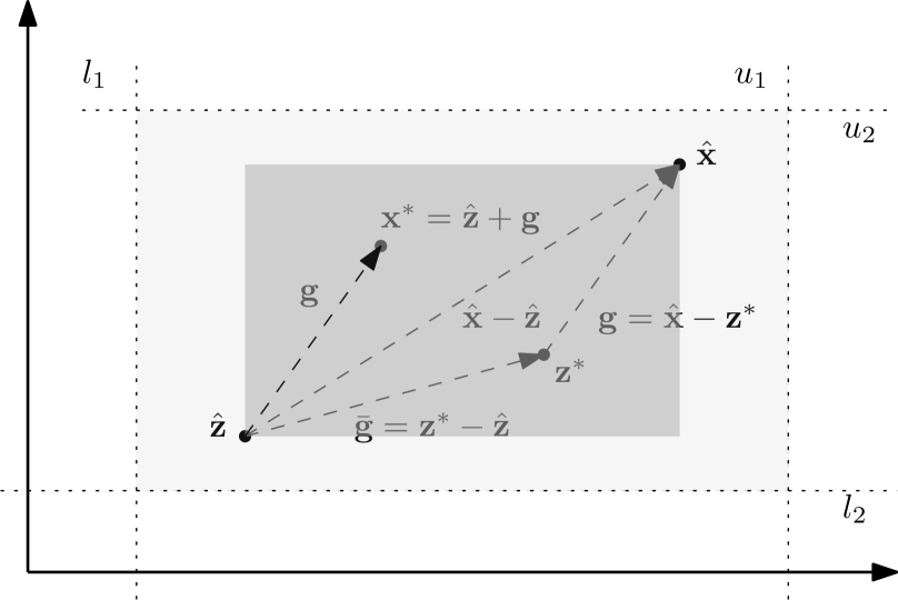
Proof
See Figure 2 for an illustration of the proof.
By Definition 5, there exists a with and .
Let and and note that , and .
Now define .
By the fact that both and lie within the bounds and and that both and are conformal to , we see that both and also lie within the bounds and .
Thus is a feasible solution of RP and is a feasible solution of IP.
We can also write
Since is a continuous optimum and is a feasible solution to RP, the left hand side is non-positive, and so is .
But since is an integer optimum it must be that is another integer optimum and thus , and subsequently and thus is another continuous optimum.
∎
Figure 2: The situation of Lemma 2: the feasible region between lower and upper bounds is the light grey rectangle; the dark grey rectangle marks the region of vectors which, when translated to , are conformal to .
The picture makes it clear that and are conformal to , and that the identity holds.
Proof (of Theorem LABEL:thm:scaling-proximity)
We will show one direction, as the other direction is symmetric.
Let be an optimum of IP.
By Definition 5 and Lemma 2, there exists an optimum to the continuous relaxation RP with
(12)
As the continuous relaxations coincide, is also an optimum to the continuous relaxation of IP-scaled.
Substituting ,
we obtain an objective-value preserving bijection between the solutions of the continuous relaxation of IP and the solutions of the continuous relaxation of IP-scaled.
In particular, is an optimum to the continuous relaxation of IP-scaled.
Again by proximity (Lemma 2), the instance IP-scaled has an optimal solution with
(13)
Substituting back, is an optimal solution to s-IP.
The claim follows by triangle inequality: .
∎
As a -scaled instance is also a -scaled instance of a -scaled instance, we get the following algorithm to solve a general IP.
The algorithm is parameterized by some upper bound on the proximity bound (see Theorem LABEL:thm:scaling-proximity).
(1)
Given an initial feasible solution , recenter the instance at , obtaining IP where is feasible.
Set .
(2)
For each , perform the following steps:
Intersect the box constraints of the -scaled instance with the proximity bounds .
Solve this instance with initial solution to optimality, and let denote the optimum.
Center the current instance at .
(3)
Output .
The bound in step (2) follows from the fact that we are viewing the /̄scaled instance as an /̄scaled instance of the /̄scaled instance where , and using in the bound of Theorem LABEL:thm:scaling-proximity.
Given an initial feasible solution , we center the original instance at which transforms its right hand side to as required.
It is clear that we need at most iterations, in each of which we apply Theorem LABEL:thm:scaling-proximity with to the bounds .
∎
Remark 1
We can somewhat decrease the number of iterations of the scaling algorithm as follows.
In each instance we have .
In the first instances , we are searching in the /̄lattice.
Let us view these instances as IP-scaled instances:
then each has and .
But then for each of them we already have , so the guaranteed bound on is satisfied even without invoking the proximity theorem.
Thus, we can skip the first iterations by initially setting , reducing the number of iterations to .
This improved number of iterations matches the bound on the number of scaling phases of the algorithm of Hochbaum [32] whose parameter is , and her proximity bound is .
4 Primal Algorithm
Theorem 1.1 is proven by instantiating the scaling algorithm of Theorem 3.1 with a new strong proximity of Klein and Reuter [40], and the standard branching algorithm for each subinstance [23, Lemma 8].
The parameter dependency of the function is essentially determined by and the proximity bound .
The currently best known bounds for both are triple-exponential in terms of [40, Corollary 2.1, Lemma 2.3], and this seems to be optimal for , see [34, Theorem 1].
Since the exact dependence of on and is not the focus of this work, we shall simply focus on proving the theorem in its stated form.
Klein and Reuter [40] (improving on Cslovjecsek et al. [14]) give a bound on independent of :
We instantiate the scaling algorithm from Theorem 1.1 as follows.
We provide Proposition 4 as an upper bound on .
We solve each of the IP instances in the scaling algorithm using the algorithm of Eisenbrand et al. [23, Lemma 8] which has running time .
Taking and the fact that for some computable function concludes the proof.
∎
5 Scaling and Sensitivity
The situation is more delicate regarding the algorithm for dual treedepth (Theorem 1.2).
Not only is there no analogue of the proximity result of Klein and Reuter [40], in fact, Cslovjecsek et al. [13, Proposition 4.1] show that there are instances of IP with small where an integer optimum is far in the /̄norm from any continuous optimum.
The proximity results for stronger relaxations [13, 45] are also of no obvious help.
Their bounds which are independent of only apply to vertex solutions, which are guaranteed to include an optimum only for linear objectives.
Moreover, solving these stronger relaxations is either not near-linear time (reliant on the ellipsoid method [45]) or limited to linear objectives [13].
Let us re-examine the scaling algorithm.
In each iteration, we go from an optimum in the lattice to an optimum in .
From the point of view of IP-scaled considering instead of means that for every we modify the separable objective function from to , the lower bound from to , and the upper bound from to .
Afterwards, we solve the new instance in the finer lattice with an initial feasible solution which was the optimum in .
Our approach for dual treedepth is to find the optimum solution in by changing the scaling factor one variable at a time.
This means that once we modify for some , we immediately solve the instance resulting from refining coordinate .
It is not clear why this should be advantageous – after all, in each iteration of the scaling algorithm we need to solve IP-scaled times instead of just once.
The advantage lies in the fact that whenever we refine a single variable, then an optimum of the refined instance is close (in terms of the -norm) to an optimum of the instance before this last refinement.
Such proximity bound will be our first contribution towards the proof of Theorem 1.2.
To show this proximity bound, we proceed in two steps.
First, we show a sensitivity theorem for changes in the box constraints .
Then, we would like to use this theorem to show that refining few variables means only a small change in the optimal solution; however, this is not possible directly, because going from to may be a big change in the absolute sense.
Thus, we use an encoding trick to circumvent this issue.
Let us start with the first step.
Theorem 5.1
Let be an optimum of IP, , and .
If the IP with replaced by is feasible, then it has an optimum with .
Proof
We will first prove the claim for the special case when is either the -th unit vector or its negation for some .
The theorem then follows by a repeated application of this claim and triangle inequality.
Specifically, we will start moving from to by gradually decreasing all the coordinates in which is smaller than .
After this step, we have a vector which is a coordinate-wise minimum of and .
The vector is feasible for all of the intermediate instances with lower bounds between and , and is feasible the instance with lower bound .
Next, we gradually increase all the coordinates in which is greater than , resulting in .
We have that is feasible for all of the intermediate steps of the second phase.
This way we see that all the intermediate instances are feasible and thus also have some optimal solution, hence the claim applies to them.
Assume for some , and let us denote the original IP instance by and the instance with by .
Let be an optimum of which is closest to (an optimum of ) in -norm.
Since , it has a conformal decomposition with , for every , and some potentially appearing with repetitions (see Proposition 3).
We claim that there can actually be at most one element in the decomposition.
For contradiction assume that there are two or more elements in the conformal decomposition of .
Our plan is to use a proof analogous to that of Lemma 2.
We will define a vector , use it to define and , and show that is feasible for and is feasible for .
This situation is a direct analogue of Figure 2, and the rest of the proof will be as well.
Let us fix some conformal decomposition of and denote the multiset by .
If there is no element such that , then which in turn means that is also feasible and in fact optimum for .
Hence, by the choice of , we have and the bound on their distance follows trivially.
Now let us consider the case when there is at least one element in with .
Set , , and accordingly and .
We claim that is still feasible for and is still feasible for .
In the case that is the only element of with , then as and , we have which finishes the claim.
Otherwise assume that there is another element of aside from with .
If is infeasible for or is infeasible for , then it only violates the respective bound by , and only in the -th coordinate.
By this observation, we have that must be feasible for even if was not, and must be feasible for even if was not.
The rest of the argument is identical to the one in the proof of Lemma 2.
We can write (in both cases)
which, using Proposition 2 with values , , , gives
(15)
Since is an optimum of the original instance and is feasible for it, the left hand side is non-positive, and so is .
But since is an optimum of the modified instance and is feasible for it, must be nonnegative, hence , thus is another optimum of the modified instance.
However, by our assumption that there are at least two elements in the decomposition, both and are non-zero, hence is closer to , a contradiction.
∎
An analogous statement to Theorem 5.1 can be proved for the upper bound :
Corollary 1
Let be an optimum of IP, , and . Assuming that the IP with replaced by is feasible, then it has an optimum satisfying .
Consider an instance of IP with .
For any , the -scaled IP is an IP instance with input and with the constraint matrix defined as follows.
If , then , and ; if , then , and .
The -th column of the constraint matrix is either twice the -th column of if , otherwise it is simply the -th column of .
We use to denote the symmetric difference of sets , i.e., .
We denote by the matrix .
Our goal is to prove the following theorem:
Theorem 5.2
Let , and let be an optimum of the -scaled IP.
Then if the -scaled IP is feasible, it has an optimum satisfying
(16)
The second inequality in Theorem 5.2 follows from the following lemma.
Lemma 3
.
Proof
Consider an element of and split it evenly into three vectors (i.e. the first components are , the next components are , and the last components are ).
Define .
We have from the “bottom half” of where .
We claim that .
For contradiction assume otherwise, meaning that can be decomposed as with and .
We will define three new vectors and we will show that , thus getting a contradiction with conformal minimality of an element of .
For set if is non-negative, and if is negative.
It is clear that .
We set and .
As is non-zero, it follows that at least one of and are non-zero, and that is non-zero.
We get that and as .
Finally from we get which yields the desired contradiction.
Thus we bound and which finishes the proof.
∎
We want to use Theorem 5.1 to prove Theorem 5.2.
In order to do that, we will construct an auxiliary IP instance which will be able to encode the -scaled instance for any by only a small change in its bounds.
Specifically the constraint matrix is exactly .
The bounds are defined as follows:
for , we set
•
and ,
•
and ,
•
if , ,
•
otherwise , then and ,
The objective function is simply .
In summary:
(aux--IP)
Given a solution of the -scaled IP, a vector intuitively encodes in the following way: if , the variable is already in the refined grid and we split its value into the least significant bit () and the rest (); otherwise if , the variable is not in the refined grid, so we just set .
Formally, if , set and , otherwise we need to distinguish whether is positive or negative: if , set and ; otherwise set and .
For each , set .
In the other direction, given a solution of the aux--IP, we construct a solution of the -scaled IP as follows.
If , set , otherwise if , set .
Notice that the value of with respect to is equal to the value of with respect to :
•
since and ,
•
since by definition.
By the construction above we immediately get:
Lemma 4
A solution of the -scaled IP is optimal if and only if the corresponding solution of aux--IP is optimal.
Let be the solution of aux--IP corresponding to the optimum from the statement.
By Lemma 4, is optimal for aux--IP.
Observe that when we replace with , the bounds of the aux--IP instance only change in coordinates , and in each coordinate of it changes by (for a coordinate in , the lower bound changes from to , and the upper bound from to , and for a coordinate in , the bounds change from or to ).
Thus, by Theorem 5.1, there exists an optimum at -distance at most .
Finally, the corresponding optimum of the -scaled IP is at the claimed distance, again, by construction.
∎
By Lemma 3, we can use asymptotically the same bounds for as ; for example, we have [23, Theorem 3].
The next lemma analogously relates and .
Lemma 5
Let be a -decomposition of . A -decomposition of with and can be computed in linear time.
Proof
Start from , and go over .
Let be the set of rows of which are non-zero in column .
Observe that all of them must lie on some root-leaf path in , and call the leaf of this path.
Attach a new leaf to , representing the row of .
It is easy to verify that is a -decomposition of .
Since we have only been attaching leaves to vertices which were leaves in , we have only possibly increased the height by , and we have only possibly added one more non-degenerate node on any root-leaf path, increasing the topological height by at most .
This shows the lemma.
∎
6 Dual algorithm
The main technical ingredient of our algorithm is a dynamic data structure solving the following subproblem: for an IP instance , its feasible solution , and a parameter , the -IP problem is to solve
(-IP)
If two -IP instances differ in at most coordinates of their bounds and objective functions, we call them -similar.
We shall construct a data structure we call “convolution tree” which maintains a representation of an -IP instance together with its optimal solution, takes linear time to initialize, and takes time roughly to update to represent a -similar -IP instance.
Before we give a definition of a convolution tree, let us first explain the problem it solves.
The -IP problem is implicitly present in the literature as an important subtask of algorithms for IP with small [30, 23].
A feasible solution to an instance of -IP should be viewed as a linear combination of columns of with coefficients given by such that the linear combination of the columns is , and the cost of the solution is .
Finding an optimum solution can be done by the following dynamic programming approach:
For simplification let us assume and that are the all (minus) infinity vectors.
For every we denote by the restriction of to coordinates in , and .
For any linear combination of any first columns of where for each we have .
The restriction on the domain of the coefficients comes from the condition in -IP.
Thus for every , and vector , we can compute the cheapest linear combination of the first columns that sums up to recursively – for every , compute the cheapest linear combination of the first columns of that sums up to , and store the that minimizes .
To bound the running time of this dynamic programming algorithm, observe that the dynamic programming table has entries and computing each of them requires time .
As we have sketched in the beginning of Section 5, the algorithm for dual treedepth will not descale all variables at once but do it one by one instead.
This is where Theorem 5.2 comes into play:
if we write the initial IP instance as an aux--IP instance with optimum (which can be computed by the dynamic programming approach described above), then the optimum of an instance where we descale one variable has the property that there exists an optimum with .
Thus computing can be viewed as solving -IP with and .
We will need to solve -IP instances in order to solve a single IP instance of the many IP instances of the scaling algorithm.
If we solve each of them using the dynamic programming approach, then in the end, the dependence on in the running time is .
Instead of solving each -IP instance from scratch, we shall leverage the fact that subsequent -IP instances in a single iteration of the scaling algorithm do not differ too much which leads to the possibility of sparse updates.
To simplify the subsequent explanation, let us now assume that the update operation only affects the functions as we can simulate the updates to the bounds and by changes to : when is updated to , we can set for every ;
we need to be careful to keep convex though so instead we set for some sufficiently large so that for every and we have .
We can handle updates of analogously.
A change in the objective function means that we change the cost of all partial solutions on columns .
A naive way to perform an update operation would be to recompute the dynamic programming table but this would take time .
The idea behind a fast update is to build an analogue of a segment tree [7] on top of the dynamic programming table.
For simplicity assume that is a power of two, otherwise we can add enough all/̄zero columns to make it so.
We build a rooted full binary tree with leaves, meaning that every internal vertex has exactly two children and we denote the root by .
Note that the height of is .
Notationally, let be at depth 0 and the leaves at depth .
We enumerate leaves of with numbers from left to right.
For each vertex we say that it represents an interval if the leaves in the subtree of rooted at have labels exactly .
For each vertex and each we shall compute the cheapest linear combinations of columns with respect to that sums up to or let the cost be if no such linear combination exists, and we denote this value by .
The computation shall be done as follows.
Let us assume that for every vertex and each we have implicitly .
For every leaf representing the interval of and every we set .
Now successively for depths and for every vertex at these depths with children and , and for every we set
(17)
The reason why we call our data structure convolution tree is that we can also view computing as a /̄convolution
(18)
We can also store the linear combination of columns whose indices are represented by a vertex that make up for every .
To retrieve the solution of -IP we need to simply query .
When a function is updated, then it is only necessary to recompute for vertices that lie on the path from the leaf of labelled by to the root.
The recomputation when is updated is done exactly as the initialization – by computing a convolution in every vertex on a root/̄leaf path from the leaf labelled .
This update only affects vertices and each convolution requires time , and the initialization takes time (ignoring dependence on parameters and ).
When we formalize the convolution tree, we shall show how to decrease the super/̄polynomial dependence on to .
The idea here is that we can leverage the sparse recursive structure of the /̄decomposition of instead of considering each column separately.
Essentially, notice that for every such that and any , the prefix sum is non/̄zero in at most coordinates, and thus can be represented very compactly.
This eventually decreases the exponent to .
Definition 6 (Convolution Tree)
Let , be a -decomposition of , , and .
A convolution tree is a data structure which stores two vectors and a separable convex function , and we call the state of .
A convolution tree supports the following operations:
1.
Init initializes to be in state .
2.
Update is defined for , and a univariate convex function .
Calling Update changes the -th coordinates of the state into and , i.e.,
if is the state of before calling Update and is the state of afterwards, then for all , , , and , and , , and .
3.
Query returns a solution sequence where is a solution of
(19)
with the -dimensional zero vector, and the current state of .
If (19) has no solution, we define its solution to be .
Each vector has a sparse representation as there are at most coordinates that are non-zero due to the constraint , and thus can be represented by a list of length of index-value pairs.
In Definition 6, the set represents the set of possible right hand sides of (19), and the extra coordinate in the set serves to represent the set of considered -norms, which includes 0, of solutions of (19).
We are being slightly opaque in the definition of Update since we are only given a comparison oracle for and not individual ’s.
However, a comparison oracle for ’s is implicit from the comparison oracle for thus we can speak about updating individual ’s.
We also introduce the following shortcut: for by /̄Update where with , , and we mean calling Update for each in increasing order of .
We present an implementation of the convolution tree in the following lemma.
We prove in Appendix 0.A that the dependence on in the running time of each operation is essentially tight in the comparison model.
Lemma 6 (Convolution Tree Lemma)
Let , and be as in Definition 6, and .
We can implement all operations so that the following holds.
1.
Init can be realized in time ,
2.
Update can be realized in time ,
3.
Query can be realized in time and the result can be represented in space .
For any the vector can be retrieved in time and represented in space .
Note that the running time of Query does not depend on .
Given Lemma 6 whose proof we postpone, we prove Theorem 1.2 as follows.
The algorithm consists of two nested loops.
The outer loop is essentially the same as the one of the scaling algorithm: we begin by setting , recentering the instance using an initial feasible solution, and setting as the optimum of the -scaled instance.
If an initial feasible solution is not given as part of the input, it can be found using Lemma 1.
Similarly to the case of Theorem 1.1, finding the initial feasible solution is the only reason why the running time has the factor.
We call each iteration of the outer loop a phase, and in each phase is decremented, a solution of the -scaled instance is obtained, until and is the optimum of the original instance.
However, the process by which the algorithm goes from to is different.
In each phase, we begin by constructing the aux--IP instance for , centered at the feasible solution derived from from the previous phase.
Each phase has steps.
In step , we begin with a solution which is optimal for the -scaled instance, that is, we have already refined coordinates through , and the task of step is to refine the -th coordinate, that is, find the optimum of the -scaled instance.
By Theorem 5.2, this optimum cannot differ from the previous one by more than in the -norm.
Call the optimum from the previous step, and the nearby optimum to be found.
The proximity bound implies that there is a step of small -norm.
We recenter the aux--IP for at , which means that we are looking for an optimum of aux--IP with an additional -norm bound .
We can do this quickly using the convolution tree as follows.
At the beginning of each phase, let , and initialize a convolution tree with the matrix , a -decomposition from Lemma 5, bounds , right hand side , objective function , and .
Then, perform the following for in increasing order of :
Let be the solution of the -IP represented by , , let , and call a -Update on to recenter its -IP at .
Now call an Update on the coordinate to change its bounds from to .
Notice that at the beginning of step , represents the aux--IP for , and since it is centered at the optimum of the aux--IP for and by Theorem 5.2 and our choice of , the optimum obtained by calling Query on is in fact the optimum of the aux--IP for .
Thus, after the -th step, the optimum of is the optimum of the aux--IP for , and we construct from it the solution used to initialize the next phase.
This, together with the correctness of the scaling algorithm, shows the correctness of the algorithm.
As for complexity, notice that there are phases, each phase has steps, each step consists of calling a -Update followed by a Query with , and one additional Update followed by a Query.
Plugging into Lemma 6 finishes the proof.
Note that similarly to the primal algorithm (Theorem 1.1), the dependence on is only necessary to find an initial feasible solution.
∎
Before we prove Lemma 6, we formalize the notion of convolution we use.
Definition 7 (Convolution)
Given a set and tuples , a tuple is the convolution of and , denoted , if
We define recursively over , then describe how the operations are realized, and finally analyze the time complexity.
If , we assume is dual block-structured along (recall Definition 3) and we have, for every , matrices and a -decomposition of with and , and a corresponding partitioning of and .
If , let , for each , and be empty.
For , , denote by the submatrix of induced by the rows and columns of the blocks , , , and be the restriction of to the coordinates of .
Observe that .
We obtain by first defining a convolution tree for each , where is a convolution tree for the matrix and for and , and then constructing a binary tree whose leaves are the ’s and which is used to join the results of the ’s in order to realize the operations of .
Since, for each , is supposed to be a convolution tree for a matrix with , if , we will construct by a recursive application of the procedure which will be described in the text starting from the next paragraph.
Now we describe how to obtain if , i.e., when is just one column.
When is initialized or updated, we construct the sequence by using the following procedure.
For each , defining to be such which satisfies and minimizes , and returning either if it is defined or if no such exists.
Notice that and are scalars.
We say that a rooted binary tree is full if each vertex has or children, and that it is balanced if its height is at most where is the number of leaves of the tree.
It is easy to see that for any number there exists a rooted balanced full binary tree with leaves.
Let be a rooted balanced full binary tree with leaves labeled by the singletons in this order, and whose internal vertices are labeled as follows: if has children , then ; hence the root satisfies and the labels are subsets of consecutive indices in .
We obtain by identifying the leaves of with the roots of the trees and will explain how to use to join the results of all ’s in order to realize the operations of .
To initialize with vectors and and a function , we shall compute, in a bottom-up fashion, the sequence described in point 3 of Definition 6.
Let be a node of and let and be the leftmost and rightmost leaves of (i.e., the subtree of rooted at ), respectively.
Moreover, if is an internal node, let its left and right child be and , respectively, and let be the rightmost leaf of .
Consider the following auxiliary problem, which is intuitively problem (19) restricted to blocks to : simply append “” to all relevant objects, namely and :
(22)
where has dimension .
Let be a solution of (22) and let be the sequence .
If is a leaf of , the sequence is obtained by querying (which was defined previously).
Otherwise, compute the sequences and for the children of , respectively.
Then, we compute a convolution of sequences, , obtained from by setting , where .
We also compute a witness of .
The desired sequence is easily obtained from .
The Update operation is realized as follows.
Let be as described in Definition 6.
Let be the index of the block containing coordinate , and let be the coordinate of block corresponding to .
First traverse downward from the root to leaf , call Update on subtree , and then recompute convolutions and sequences for each vertex on a root-leaf path starting from the leaf and going towards the root.
Let us analyze the time complexity.
The convolution tree is composed of levels of smaller convolution trees, each of which has height .
Specifically, the topmost level consists of the nodes corresponding to the internal vertices of , and the previous levels are defined analogously by recursion (e.g., level consists of the union of the topmost levels of over all , etc.).
Thus, .
There are leaves of , one for each column of .
The initialization of leaves takes time at most .
Let , , denote the number of internal nodes at level .
Because a full binary tree has at most as many internal nodes as it has leaves, we see that .
Then, initializing level amounts to solving convolutions and their witnesses, each of which is computable in time .
Processing level amounts to solving convolutions with sets where is obtained from by dropping some coordinates, and thus , and hence computing one convolution can be done in time .
In total, initialization takes time at most .
Regarding the Update operation, there is one leaf of corresponding to the coordinate being changed.
Thus, in order to update the results, we need to recompute all convolutions corresponding to internal nodes along the path from the leaf to the root.
Because , the number of such nodes is , with each taking time at most .
As the output of Query has a sparse representation described in the statement of the lemma, the running time for Query follows.
∎
Open Problems
Our results primarily point in two interesting research directions.
First, is it possible to eliminate the factor in the dual algorithm (Theorem 1.2), at least for some classes of IP with small ?
If not, how could the lower bound be strengthened to match our results?
Second, the lower bound does not apply outside of the comparison oracle model; for which classes of objectives beyond linear can one design faster, possibly strongly polynomial algorithms?
{credits}
6.0.1 Acknowledgements
Hunkenschröder acknowledges support by the Einstein Foundation Berlin.
Levin is partially supported by ISF - Israel Science Foundation grant number 1467/22.
Koutecký and Vu are partially supported by Charles Univ. project UNCE 24/SCI/008, by the ERC-CZ project LL2406 of the Ministry of Education of Czech Republic.
Koutecký is additionally supported by projects 22-22997S and 25-17221S of GA ČR, Vu by the project 24-10306S of GA ČR.
Appendix 0.A Optimality of the Convolution Tree
In this section we argue that our realization of the convolution tree (Lemma 6) is optimal with respect to .
Formally, we prove the following lemma.
Lemma 7
In any implementation of the convolution tree in the comparison model, the total running time of one operation Init, operations Update and operations Query requires time .
Proof
We prove this lemma by demonstrating how to sort an array of integers using the convolution tree with one Init, Updates and Queries.
We guide ourselves with the following IP instance.
Let be integer variables.
Let be a constant larger than .
The IP instance shall be
Note that this instance has dual treedepth and .
We initialize a convolution tree with and .
We will find an optimum solution by starting from a feasible solution .
For let be a vector which has only two non-zero entries, at index it has a and at index it has .
It is easy to see that the only minimum augmenting steps are .
(Indeed, this is exactly the relevant subset of the Graver basis of mentioned in the previous section.)
We start by looking for an augmenting step as in -IP with by performing a Query operation on .
Clearly each can be sparsely represented.
At the beginning, the augmenting step that decreases the minimized objective function the most is where is the index of the maximum element of .
We apply Update on to re-center the instance at .
If we look for another augmenting step, we cannot use the same augmenting step as the constraint has become tight.
Thus the next augmenting step will be where corresponds to the second largest entry among , and so on when we search for .
Eventually the sequence of augmenting steps returned by has the property that is the index of the -th largest entry of .
Thus we have listed in non-increasing order.
Our instance has , hence Init takes time , Update time , and Query time .
In total, we used one Init, Updates, and Queries.
If we could perform this combination of operations in time , then we would get a contradiction with the known fact that sorting requires time in the comparison model.
Note that we only copy ’s, thus our lower bound indeed works in the comparison model.
In particular, the convolutions that occur never involve the numbers .
This concludes the proof.
∎
References
[1]
Achterberg, T., Bixby, R.E., Gu, Z., Rothberg, E., Weninger, D.: Presolve
reductions in mixed integer programming. INFORMS J. Comput.
32(2), 473–506 (2020)
[2]
Ahuja, R.K., Magnanti, T.L., Orlin, J.B.: Network Flows. Prentice Hall, Inc.,
Englewood Cliffs, New Jersey (1993)
[3]
Alumur, S.A., Kara, B.Y.: Network hub location problems: The state of the art.
European Journal of Operational Research 190(1), 1–21 (2008)
[4]
Anderson, R., Huchette, J., Ma, W., Tjandraatmadja, C., Vielma, J.P.: Strong
mixed-integer programming formulations for trained neural networks. Math.
Program. 183(1), 3–39 (2020)
[5]
Asahiro, Y., Jansson, J., Miyano, E., Ono, H., Zenmyo, K.: Approximation
algorithms for the graph orientation minimizing the maximum weighted
outdegree. J. Comb. Optim. 22(1), 78–96 (2011)
[6]
Aschenbrenner, M., Hemmecke, R.: Finiteness theorems in stochastic integer
programming. Found. Comput. Math. 7(2), 183–227 (2007)
[7]
de Berg, M., Cheong, O., van Kreveld, M.J., Overmars, M.H.: Computational
geometry: algorithms and applications, 3rd Edition. Springer (2008)
[8]
Bertsimas, D., King, A., Mazumder, R.: Best subset selection via a modern
optimization lens. The Annals of Statistics 44(2), 813–852 (2016)
[9]
van den Briel, M., Vossen, T., Kambhampati, S.: Reviving integer programming
approaches for AI planning: A branch-and-cut framework. In: Automated
Planning and Scheduling, ICAPS 2005. Proceedings. pp. 310–319. AAAI
(2005)
[10]
Chen, L., Kyng, R., Liu, Y.P., Meierhans, S., Gutenberg, M.P.: Almost-linear
time algorithms for incremental graphs: Cycle detection, sccs, s-t shortest
path, and minimum-cost flow. In: Mohar, B., Shinkar, I., O’Donnell, R. (eds.)
Proceedings of the 56th Annual ACM Symposium on Theory of Computing, STOC
2024, Vancouver, BC, Canada, June 24-28, 2024. pp. 1165–1173. ACM (2024)
[11]
Chen, L., Kyng, R., Liu, Y.P., Peng, R., Gutenberg, M.P., Sachdeva, S.: Maximum
flow and minimum-cost flow in almost-linear time. In: 63rd IEEE Annual
Symposium on Foundations of Computer Science, FOCS 2022, Denver, CO, USA,
October 31 - November 3, 2022. pp. 612–623. IEEE (2022)
[12]
Chen, L., Marx, D., Ye, D., Zhang, G.: Parameterized and approximation results
for scheduling with a low rank processing time matrix. In: 34th Symposium on
Theoretical Aspects of Computer Science, STACS 2017. LIPIcs, vol. 66, pp.
22:1–22:14. Schloss Dagstuhl — Leibniz-Zentrum für Informatik (2017)
[13]
Cslovjecsek, J., Eisenbrand, F., Hunkenschröder, C., Rohwedder, L.,
Weismantel, R.: Block-structured integer and linear programming in strongly
polynomial and near linear time. In: 32nd Annual ACM-SIAM Symposium on
Discrete Algorithms, SODA 2021. pp. 1666–1681. SIAM (2021)
[14]
Cslovjecsek, J., Eisenbrand, F., Pilipczuk, M., Venzin, M., Weismantel, R.:
Efficient sequential and parallel algorithms for multistage stochastic
integer programming using proximity. In: 29th Annual European Symposium on
Algorithms, ESA 2021. LIPIcs, vol. 204, pp. 33:1–33:14. Schloss Dagstuhl
— Leibniz-Zentrum für Informatik (2021)
[15]
Cslovjecsek, J., Koutecký, M., Lassota, A., Pilipczuk, M., Polak, A.:
Parameterized algorithms for block-structured integer programs with large
entries. In: Woodruff, D.P. (ed.) Proceedings of the 2024 ACM-SIAM
Symposium on Discrete Algorithms, SODA 2024, Alexandria, VA, USA, January
7-10, 2024. pp. 740–751. SIAM (2024)
[16]
De Loera, J.A., Hemmecke, R., Köppe, M.: Algebraic and Geometric Ideas
in the Theory of Discrete Optimization, MOS-SIAM Series on Optimization,
vol. 14. SIAM (2013)
[17]
De Loera, J.A., Hemmecke, R., Onn, S., Weismantel, R.: -fold integer
programming. Discrete Optimization 5(2), 231–241 (2008), in
Memory of George B. Dantzig
[18]
Dong, S., Goranci, G., Li, L., Sachdeva, S., Ye, G.: Fast algorithms for
separable linear programs. In: Woodruff, D.P. (ed.) Proceedings of the 2024
ACM-SIAM Symposium on Discrete Algorithms, SODA 2024, Alexandria, VA,
USA, January 7-10, 2024. pp. 3558–3604. SIAM (2024)
[19]
Dong, S., Lee, Y.T., Ye, G.: A nearly-linear time algorithm for linear programs
with small treewidth: a multiscale representation of robust central path. In:
Khuller, S., Williams, V.V. (eds.) STOC ’21: 53rd Annual ACM SIGACT
Symposium on Theory of Computing, Virtual Event, Italy, June 21-25, 2021. pp.
1784–1797. ACM (2021)
[20]
Eisenbrand, F., Hunkenschröder, C., Klein, K.: Faster algorithms for
integer programs with block structure. In: 45th International Colloquium on
Automata, Languages, and Programming, ICALP 2018. LIPIcs, vol. 107, pp.
49:1–49:13. Schloss Dagstuhl — Leibniz-Zentrum für Informatik (2018)
[21]
Eisenbrand, F., Hunkenschröder, C., Klein, K., Koutecký, M., Levin,
A., Onn, S.: An algorithmic theory of integer programming. CoRR
abs/1904.01361 (2019)
[22]
Eisenbrand, F., Hunkenschröder, C., Klein, K., Koutecký, M., Levin,
A., Onn, S.: Reducibility bounds of objective functions over the integers.
Oper. Res. Lett. 51(6), 595–598 (2023)
[23]
Eisenbrand, F., Hunkenschröder, C., Klein, K.M., Koutecký, M., Levin, A.,
Onn, S.: Sparse integer programming is fixed-parameter tractable. Mathematics
of Operations Research 0(0) (2024)
[24]
Eisenbrand, F., Rothvoss, T.: A parameterized linear formulation of the integer
hull. CoRR abs/2501.02347 (2025)
[25]
Floudas, C.A., Lin, X.: Mixed integer linear programming in process scheduling:
Modeling, algorithms, and applications. Ann. Oper. Res. 139(1),
131–162 (2005)
[26]
Gavenčiak, T., Koutecký, M., Knop, D.: Integer programming in
parameterized complexity: Five miniatures. Discret. Optim.
44(Part), 100596 (2022)
[27]
Graver, J.E.: On the foundations of linear and integer linear programming i.
Math. Program 9(1), 207–226 (1975)
[28]
Grötschel, M., Lovász, L., Schrijver, A.: Geometric algorithms and
combinatorial optimization, Algorithms and Combinatorics, vol. 2.
Springer-Verlag, Berlin, second edn. (1993)
[29]
Hemmecke, R., Köppe, M., Weismantel, R.: Graver basis and proximity
techniques for block-structured separable convex integer minimization
problems. Mathematical Programming 145(1-2, Ser. A), 1–18 (2014)
[30]
Hemmecke, R., Onn, S., Romanchuk, L.: -fold integer programming in cubic
time. Math. Program. 137(1-2), 325–341 (2013)
[31]
Hemmecke, R., Schultz, R.: Decomposition of test sets in stochastic integer
programming. Mathematical Programming 94, 323–341 (2003)
[32]
Hochbaum, D.S.: Lower and upper bounds for the allocation problem and other
nonlinear optimization problems. Math. Oper. Res 19(2), 390–409
(1994)
[33]
Hochbaum, D.S., Shanthikumar, J.G.: Convex separable optimization is not much
harder than linear optimization. Journal of the ACM 37(4),
843–862 (1990)
[34]
Hunkenschröder, C., Klein, K., Koutecký, M., Lassota, A., Levin,
A.: Tight lower bounds for block-structured integer programs. In: Vygen, J.,
Byrka, J. (eds.) Integer Programming and Combinatorial Optimization - 25th
International Conference, IPCO 2024, Wroclaw, Poland, July 3-5, 2024,
Proceedings. Lecture Notes in Computer Science, vol. 14679, pp. 224–237.
Springer (2024)
[35]
Jansen, K., Klein, K., Lassota, A.: The double exponential runtime is tight for
2-stage stochastic ILPs. Math. Program. 197(2), 1145–1172
(2023)
[36]
Jansen, K., Klein, K., Maack, M., Rau, M.: Empowering the configuration-IP:
new PTAS results for scheduling with setup times. Math. Program.
195(1), 367–401 (2022)
[37]
Jansen, K., Lassota, A., Rohwedder, L.: Near-linear time algorithm for -fold
ILPs via color coding. SIAM J. Discret. Math. 34(4),
2282–2299 (2020)
[38]
Karp, R.M.: Reducibility among combinatorial problems. In: Miller, R.E.,
Thatcher, J.W., Bohlinger, J.D. (eds.) Complexity of Computer Computations,
The IBM Research Symposia Series, pp. 85–103. Springer (1972)
[39]
Klein, K.: About the complexity of two-stage stochastic IPs. Math. Program.
192(1), 319–337 (2022)
[40]
Klein, K., Reuter, J.: Collapsing the tower — On the complexity of
multistage stochastic IPs. In: 33rd Annual ACM-SIAM Symposium on Discrete
Algorithms, SODA 2022. pp. 348–358. SIAM (2022)
[41]
Knop, D., Koutecký, M., Levin, A., Mnich, M., Onn, S.: Multitype integer
monoid optimization and applications. CoRR abs/1909.07326 (2019)
[42]
Knop, D., Koutecký, M., Levin, A., Mnich, M., Onn, S.: High-multiplicity
n-fold ip via configuration lp. Mathematical Programming 200(1),
199–227 (Jun 2023)
[43]
Knop, D., Koutecký, M.: Scheduling meets -fold integer programming. J.
Sched. 21(5), 493–503 (2018)
[44]
Knop, D., Koutecký, M., Levin, A., Mnich, M., Onn, S.: Parameterized
complexity of configuration integer programs. Oper. Res. Lett.
49(6), 908–913 (2021)
[45]
Knop, D., Koutecký, M., Levin, A., Mnich, M., Onn, S.: High-multiplicity
-fold IP via configuration LP. Math. Program. 200(1),
199–227 (2023)
[46]
Knop, D., Koutecký, M., Mnich, M.: Combinatorial -fold integer
programming and applications. Math. Program. 184(1), 1–34 (2020)
[47]
Knop, D., Koutecký, M., Mnich, M.: Voting and bribing in
single-exponential time. ACM Trans. Economics and Comput. 8(3),
12:1–12:28 (2020)
[48]
Knop, D., Pilipczuk, M., Wrochna, M.: Tight complexity lower bounds for integer
linear programming with few constraints. ACM Trans. Comput. Theory
12(3), 19:1–19:19 (2020)
[49]
Knueven, B., Ostrowski, J., Watson, J.: On mixed-integer programming
formulations for the unit commitment problem. INFORMS J. Comput.
32(4), 857–876 (2020)
[50]
Koutecký, M., Levin, A., Onn, S.: A parameterized strongly polynomial
algorithm for block structured integer programs. In: Proc. ICALP 2018.
Leibniz Int. Proc. Informatics, vol. 107, pp. 85:1–85:14 (2018)
[51]
Lau, L.C., Ravi, R., Singh, M.: Iterative methods in combinatorial
optimization, vol. 46. Cambridge University Press (2011)
[52]
Lodi, A., Martello, S., Monaci, M.: Two-dimensional packing problems: A
survey. European Journal of Operational Research 141(2), 241–252
(2002)
[53]
Murota, K., Tamura, A.: Proximity theorems of discrete convex functions. Math.
Program. 99(3), 539–562 (2004)
[54]
Norton, C.H., Plotkin, S.A., Tardos, É.: Using separation algorithms in
fixed dimension. J. Algorithms 13(1), 79–98 (1992)
[55]
Onn, S.: Nonlinear discrete optimization. Zurich Lectures in Advanced
Mathematics, European Mathematical Society (2010)
[56]
Reidl, F., Rossmanith, P., Villaamil, F.S., Sikdar, S.: A faster parameterized
algorithm for treedepth. In: Esparza, J., Fraigniaud, P., Husfeldt, T.,
Koutsoupias, E. (eds.) Proceedings Part I of the 41st International
Colloquium on Automata, Languages, and Programming, ICALP 2014, Copenhagen,
Denmark, July 8-11, 2014. Lecture Notes in Computer Science, vol. 8572, pp.
931–942. Springer (2014)
[57]
Schultz, R., Stougie, L., van der Vlerk, M.H.: Two-stage stochastic integer
programming: a survey. Statistica Neerlandica 50(3), 404–416
(1996)
[58]
Toth, P., Vigo, D. (eds.): The Vehicle Routing Problem. Society for Industrial
and Applied Mathematics, Philadelphia, PA, USA (2001)
[59]
Vossen, T., Ball, M.O., Lotem, A., Nau, D.S.: On the use of integer programming
models in AI planning. In: International Joint Conference on Artificial
Intelligence, IJCAI 99. Proceedings. pp. 304–309. Morgan Kaufmann (1999)