Physics-inspired Generative AI models via real hardware-based noisy quantum diffusion

Abstract

Quantum Diffusion Models (QDMs) are an emerging paradigm in Generative AI that aims to use quantum properties to improve the performances of their classical counterparts. However, existing algorithms are not easily scalable due to the limitations of near-term quantum devices. Following our previous work on QDMs, here we propose and implement two physics-inspired protocols. In the first, we use the formalism of quantum stochastic walks, showing that a specific interplay of quantum and classical dynamics in the forward process produces statistically more robust models generating sets of MNIST images with lower Fréchet Inception Distance (FID) than using totally classical dynamics. In the second approach, we realize an algorithm to generate images by exploiting the intrinsic noise of real IBM quantum hardware with only four qubits. Our work could be a starting point to pave the way for new scenarios for large-scale algorithms in quantum Generative AI, where quantum noise is neither mitigated nor corrected, but instead exploited as a useful resource.

1 Introduction

Generative Artificial Intelligence (GenAI) is one of the most interesting recent research fields that uses Machine Learning (ML) models capable of learning the underlying structure from a finite set of samples to create new, original and meaningful content such as images, text, or other forms of data. Nowadays, GenAI technology is used both in academic and industrial applications to find new, creative, and efficient solutions to real-life problems. Over the years, different generative models have been proposed such as Generative Adversarial Networks [1], Variational Auto-Encoders [2] and Normalizing Flows  [3], which have shown great success in generating high-quality novel data. However, Denoising Probabilistic Diffusion Models  [4, 5] (or simply Diffusion Models) have recently achieved state-of-the-art performance by overcoming previous models in generative tasks, for instance, in images and audio synthesis [6, 7, 8]. DMs have been introduced by Sohl-Dickstein et al. [4] and are inspired by the physical phenomenon of non-equilibrium thermodynamics, i.e. diffusion. The generic pipeline of DMs consists of two Markov chains that are called forward (or diffusion) and backward (or denoising). In the forward chain, classical noise is injected by means of a stochastic process into the training samples until they become totally noisy. In the backward chain, Artificial Neural Networks are trained to iteratively remove the aforementioned perturbation to reverse the forward process, so as to learn the unknown distribution of the training samples and thus generate new samples. Currently, DMs are widely adopted in computer vision tasks [9, 10, 11], text generation [12], sequential data modeling [13], audio synthesis [8], and are one of the fundamental elements of famous and widespread GenAI technologies such as Stable Diffusion [14], DALL-E 4 [15] and Diffwave [8].

On the other hand, quantum computing is a rapidly emerging technology that harnesses peculiar quantum mechanical phenomena such as superposition, entanglement and coherence to solve complex problems with fewer resources or that are untractable with classical (super)computers. For instance, milestone quantum algorithms such as Shor’s factorization [16, 17] and Grover’s search [18] have exponential and quadratic speed-ups, respectively, over their classical counterparts. Moreover, quantum computing promises to achieve a speed-up in simulating quantum systems [19, 20, 21], solving linear systems of equations [22], and optimization tasks [23, 24]. However, these algorithms require fault-tolerant quantum processors [25], i.e. hardware with a large number of error-corrected qubits. Consequently, they are not feasible on currently available Noisy Intermediate-Scale Quantum (NISQ) devices [26] that use Quantum Processing Units [27, 28] composed of a few hundreds of qubits highly prone to quantum noise. In order to reduce the effects of noise, quantum error correction techniques can be applied, which, however, require an elevated number of physical qubits [29, 30]. In this context, Google Quantum AI has recently developed a new quantum device called Willow that seems to allow exponential reduction of errors while increasing the number of qubits [31].

An active area of research in quantum computation involves algorithms based on Quantum Walks. QWs have been formally introduced by Aharonov et al. [32] as the quantum mechanical counterpart of Classical Random Walks and are exploited in many quantum protocols today. It has been shown that QWs outperform CRWs, for example, in search algorithms [33, 34, 35], transport phenomena [36, 37, 38], secure communications and cryptography protocols [39, 40], and distinguishing hard graphs [41]. QWs can also be used as a primitive of a universal model for quantum computation [42, 43, 44] and can be implemented efficiently by physical experiments [45, 46, 47] and quantum processors [48, 49, 50].

QWs are part of a more general family: Quantum Stochastic Walks [51] allowing one to describe the evolution of a quantum mechanical walker by means of quantum stochastic equations of motion and to generalize also classical random walkers.

Quantum Machine Learning (QML) is an emerging field that integrates quantum computing and ML techniques [52, 53, 54]. However, due to the limitation of NISQ devices, many QML algorithms are usually applied to toy problems where data are reduced in terms of the number of features, or integrated with classical models implementing the so-called hybrid quantum-classical algorithms (or NISQ algorithms) [55, 56]. Recently, a plethora of these algorithms have been proposed in different applications, for example: image processing [57, 58], quantum chemistry [59, 60], combinatorial and optimization problems [61], searching algorithms [62], machine learning tasks [63]. In the context of Quantum Generative Artificial Intelligence (QGenAI), previous works generalize classical GenAI models into the quantum domain: Quantum Generative Adversarial Networks [64, 65], QVAE [66], and Quantum Diffusion Models [67]. An interesting aspect of QGenAI models is that they allow the integration of computational protocols with physical quantum devices. For example, QGANs have recently been realized using a silicon quantum photonic chip  [68]. Moreover, a practical quantum advantage in generative modeling has been demonstrated in the data-limited scenario, comparing quantum-against-classical generative algorithms [69].

Concerning QDMs, numerical simulations show how the design of quantum-classical algorithms can improve the quality of generated data [70, 71], learn complex quantum distributions [72], reduce the number of trainable parameters in the denoising ANN [73], and potentially achieve sampling speeds faster than those of classical DMs [74]. However, one of the main challenges of these algorithms is their scalability on near-term quantum processors. In fact, the currently proposed QDMs approaches are usually implemented in simplified scenarios [67, 75, 76], or using pre-processing techniques [70] and classical latent models [77] to reduce the dimensional representation of the data. In addition, the idea of harnessing quantum noise to corrupt data in the forward diffusion process has been explored in simulated scenarios through quantum noise channels [67, 76, 78].

In this work, we first study the performances in image generation of DMs when classical diffusion is replaced or integrated with quantum stochastic dynamics in the forward process. In particular, using the formalism of QSWs we show that a specific interplay of quantum-classical stochastic dynamics improves image generation quality, leading to lower Fréchet inception distance (FID) values between real and generated samples, and the hybrid model is also statistically more robust than the classical DMs. Then, in the second part we implement a QW dynamics on quantum circuit and exploit the intrinsic noise of a real IBM quantum processor to generate the MNIST dataset.

2 Results

2.1 Quantum, hybrid and classical stochastic diffusion

In classical DMs, the forward process maps an unknown initial data distribution $q(\mathbf{x}_{0})$ into a final well-known distribution $\pi(\mathbf{x}_{T})$ by a Markov chain that transforms the initial samples $\mathbf{x}_{0}\sim q(\mathbf{x}_{0})$ into pure noise samples $\mathbf{x}_{T}\sim\pi(\mathbf{x}_{T})$ after $T$ time steps. In this process, the features of the samples are mathematically represented as classical random walkers undergoing stochastic dynamics [5]. For a more detailed description of the DMs, see Section 4.

Next, we consider the family of DMs for discrete categorical data. In this framework, a sample is a discrete scalar $K$-categorical random variable $X$ that takes the value $x_{t}\in 1,\dots,K$ at the time step $t\in[0,T]$ [12, 79]. In the following, we denote by $\mathbf{x}$ the one-hot version of $x$, that is, a vector whose elements for the category $k$ are $x_{k}=1$ and $x_{j}=0$ for $j\not=k$. In the forward, the sample $\mathbf{x}_{t}$ at time $t$ is obtained drawing from the transition kernel:

$$\mathbf{x}_{t} \sim q(\mathbf{x}_{t}|\mathbf{x}_{t-1}),$$ (1)

$$q(\mathbf{x}_{t}|\mathbf{x}_{t-1}) =\text{Cat}(\mathbf{x}_{t};\mathbf{p}=\mathbf{x}_{t-1}\mathbf{Q}_{t}),$$ (2)

where Cat$(\mathbf{x};\mathbf{p})$ is the categorical distribution sampling the one-hot row vector $\mathbf{x}$ with probability $\mathbf{p}$, $\mathbf{x}_{t-1}$ is the sample at time $t-1$, and $\mathbf{Q}_{t}$ is the matrix that contains the transition probabilities of $X$ from one category to another one at time $t$. The diffusion transition chain after $T$ time steps is given by:

$$q(\mathbf{x}_{0:T})=\prod_{t=1}^{T}q(\mathbf{x}_{t}|\mathbf{x}_{t-1}).$$ (3)

In Fig. 1 we show an example of the forward and backward process for a $3$-categorical random variable $X$. For a further description, see Section 4.

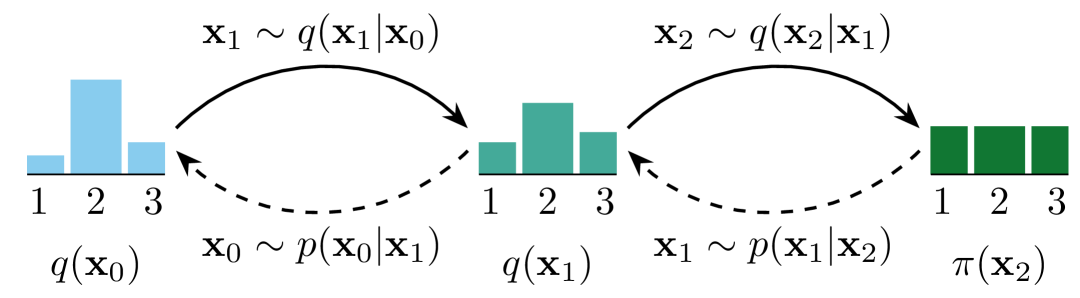
Figure 1: Example of DMs for discrete data. An initial data distribution $q(\mathbf{x}_{0})$ is transformed into a uniform categorical distribution $\pi(\mathbf{x}_{2})$ after $T=2$ time steps. The forward transition kernel is $q(\mathbf{x}_{t}|\mathbf{x}_{t-1})$, while $p(\mathbf{x}_{t-1}|\mathbf{x}_{t})$ is the transition kernel of the backward process obtained by training an ANN.

In this section, we study the performance in the image generation task when the classical stochastic dynamics in the forward chain are replaced or interplay with quantum stochastic diffusion processes. For this purpose, we decide to adopt the formalism of QSWs that provides a useful tool to study the transition from classical to quantum diffusion dynamics. This decision is inspired by previous works where the QSW formalism is used to find an optimal mixing of classical and quantum dynamics for information transport [36, 37, 38].

Formally, a continuous-time QSW dynamics is described by the Kossakowski–Lindblad-Gorini master equation [80, 81, 82]:

$$\frac{d\rho}{dt}=(1-\omega)i[H,\rho]+\omega\sum_{j}L_{j}\rho L_{j}^{\dagger}-\frac{1}{2}\{L_{j}L_{j}^{\dagger},\rho\},$$ (4)

where $\rho$ is the walker density matrix, $H$ is the Hamiltonian of the system describing the coherent evolution, and $L_{j}$ are Lindblad operators responsible for the incoherent dynamics, which represent the interactions of the system with an external environment. The continuous parameter $\omega\in[0,1]$ quantifies the interaction between coherent and incoherent evolution. For $\omega=0$, Eq. 4 describes the evolution of a pure QW. Instead, setting $\omega=1$ and choosing $L_{ij}=S_{ij}\outerproduct{i}{j}$, Eq. 4 describes the motion of a CRW where $\ket{i}$ is the quantum basis state associated with node $i$ of a graph and $S_{ij}$ is the transition matrix of the walker from node $j$ to $i$. A more complete description on QWs and CRWs is given in Section 4.

In the following, a categorical data sample is represented by a quantum stochastic walker that evolves on a cycle graph of $8$ nodes, which represent the categories of the sample. In this approach, the density operator $\rho$ of Eq. 4 describes the state evolution of the walker on the graph: the diagonal elements $\rho_{ii}$ give the probabilities that the walker is at the node $i$, while the off-diagonal elements $\rho_{ij}$ describe and contain information on the peculiar quantum mechanical effects (coherence) during the diffusion process. Next, we refer to the diagonal and off-diagonal elements of the density matrix $\rho$, respectively, as populations and coherences.

In Fig. 2 we show the evolution of the Kullback–Leibler (KL) divergence between the populations of the quantum stochastic walker on a cycle graph of $8$ nodes and the corresponding uniform distribution for different values of $\omega$. In particular, we can observe that for pure quantum diffusion dynamics ($\omega=0$) the KL divergence manifests an oscillating behavior, while in the classical case $(\omega=1)$ it smoothly converges to zero. In hybrid scenarios, with $\omega\in(0,1)$, the presence of the incoherent term of Eq. 4 dampens the oscillations of the pure quantum case, leading to faster convergence with respect to the classical case, for example, for $\omega=0.4,0.6$.

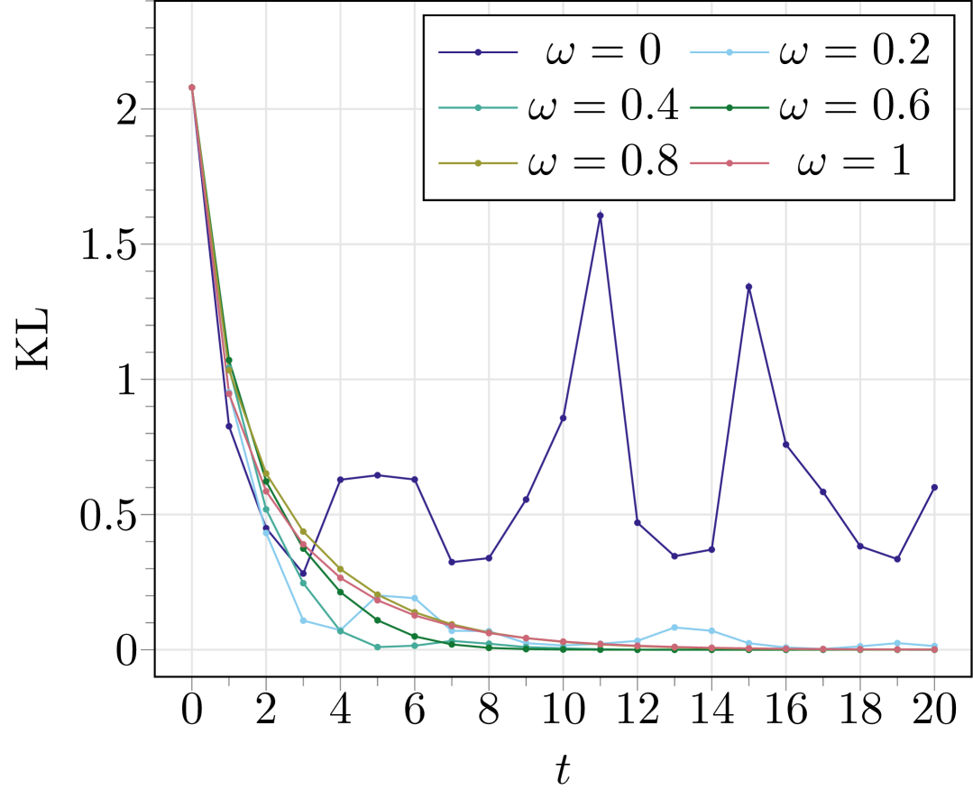
Figure 2: The KL divergence between the populations of a single QSW and the uniform distribution on a cycle graph of $8$ nodes for different value of $\omega$ after $T=20$ time steps. The walker is initially in the node $0$, corresponding to the state $\rho=\outerproduct{0}{0}$, and its evolution over the graph is obtained by solving the equation Eq. 4.

2.2 Image generation

Starting from the results of the previous section, a natural question arises: How do the different QSWs dynamics impact the generation of new samples? To answer this question, we choose to perform image generation on the MNIST [83] dataset, scaling the pixel grayscale levels from $[0,255]$ to $[0,7]$. We propose a forward dynamics, illustrated in Fig. 3, where each pixel of the image is an independent QSW on a cycle graph of $8$ nodes (one for each gray intensity value of the pixel).

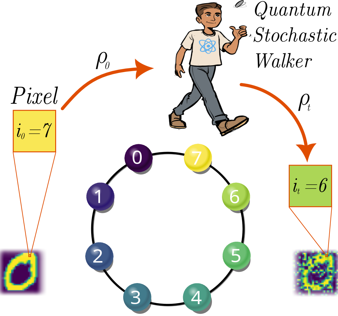
Figure 3: Illustration of the model. Each pixel of an image sample represents an independent quantum stochastic walker moving on a cycle graph of $8$ nodes that correspond to the gray intensity values. The walker moves on the graph by Eq. 4.

For simplicity, in the following we describe the forward process procedure for a single QSW. The walker is initially at the node $i_{0}$, where $i_{0}=0,1,\dots,7$, and is described by the quantum state $\rho_{0}=\outerproduct{i_{0}}{i_{0}}$. Subsequently, the state of the walker evolves by Eq. 4, and we collect the populations of the states $\rho_{1},\dots,\rho_{T}$, and use them to define categorical distributions of the forward from which we sample the positions of the walker at each time step:

$$i_{t} \sim\text{Cat}(\mathbf{p}=\text{diag}(\rho_{t-1})),$$ (5)

$$\rho_{t} =\outerproduct{i_{t}}{i_{t}},$$ (6)

where $i_{t}$ is the walker position on the graph at time $t$, and $\rho_{t}$ the corresponding quantum state. The backward process is implemented with a Multilayer Perceptron (MLP) that takes as input the one-hot encoding of the positions of the walkers at time $t$ for all pixels of the image, and is trained to predict the position at time $t-1$ for them. For details on the model, the loss function, and the training procedure, see Section 4.

In order to evaluate the generation performances for different quantum stochastic dynamics, we compute the FID metric [84] that assesses the quality of images created by a generative model. More precisely, the FID metric calculates the distance between the original and the generated datasets, and is given by:

$$\text{FID}=||\mu-\mu^{\prime}||^{2}_{2}+\tr(\Sigma+\Sigma^{\prime}-2(\Sigma\Sigma^{\prime})^{\frac{1}{2}}),$$ (7)

where $\mu$ and $\mu^{\prime}$ are, respectively, the mean of the multivariate normal distribution of the features of the original and generated image dataset, with $\Sigma$ and $\Sigma^{\prime}$ the corresponding variances. A higher value of FID indicates a poorer performance of the generative model. Moreover, to statistically assess the performance of different models, we implement $10$ simulations for each value of $\omega\in\{0,0.1,0.2,\dots,1\}$, and report in Fig. 4 the box plot visualization of the FID values of the generated digit $0$ (box plots require at least $5$ samples to provide solid statistical information [85]).

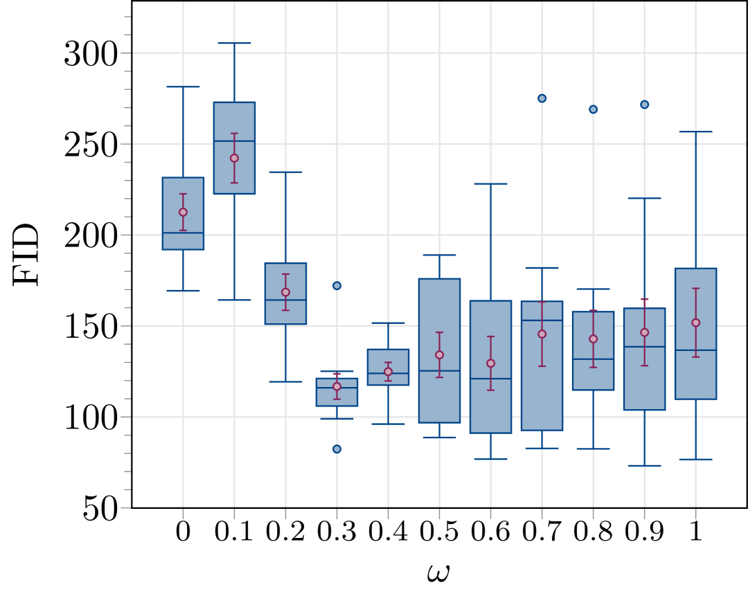
Figure 4: The box plot of FID value for different value of $\omega$. Every box plot is obtained from $10$ different repetitions of for the same value of $\omega$ with $T=20$, $8$-cycle graph. Mean and standard error of the mean are also reported. The plot show how the hybrid quantum-classical diffusion dynamics $(\omega=0.3)$ results to generate statistically better image datasets.

We observe that for a hybrid quantum-classical stochastic dynamics ($\omega=0.3$), the mean value of the FID is lower than in the classical case ($\omega=1$). Moreover, the box plot shows that in the hybrid scenario the FID values of the $10$ simulations are closely distributed around the median, while in the classical case most of the FID values are above it. In addition, all simulations for $\omega=0.3$, except for the single upper outlier, result in better FIDs than half of the runs for $\omega=1$. This means that the model with a specific interplay of quantum-classical dynamics is able to steadily generate better samples and is also statistically more robust than the classical one.

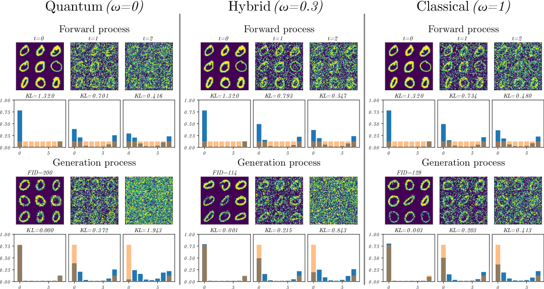
Figure 5: Image generation with QSW-based DMs via a quantum ($\omega=0$), hybrid $(\omega=0.3)$ and a classical ($\omega=1$) forward chain of $T=20$ time steps. We use the models with the inferior median values of FID between the 10 repetitions of Fig. 4. We report the first two steps of the forward chain (in the first row) of 9 different samples, and the evolution of the distribution of the pixel values for the entire dataset of digits $0$ of MNIST (blue bins in the second row) that is compared with the final uniform prior (orange bins in the second row). The KL divergence value between the two distributions is reported on the top. We also illustrate the final two steps of 9 generated samples, and the FID score between the entire training dataset and generated dataset is reported (third row). In the last row, we compare the distribution of the pixel values of the entire generated dataset (blue) with the training dataset distribution (orange), and KL divergence between them.

Finally, in Fig. 5 we show $9$ random samples of generated images of the digit $0$ using quantum, hybrid and classical stochastic dynamics.

2.3 Implementation on NISQ Devices

A hybrid QSW dynamics can be interpreted as a QW interacting with an external environment introducing noise. In this section, we therefore perform image generation by implementing a QW that exploits the intrinsic noise of a NISQ device in the forward process. This dynamic is efficiently implemented on a cycle graph with the quantum circuit of Razzoli et al. [50]. The efficiency of the algorithm allows us to modulate the amount of noise introduced in the forward chain, which has low values by default and is increased by delays. As in Section 2.2, we represent each pixel by a QW moving on a cycle graph of $8$ nodes. Furthermore, the rotation-invariant property of the cycle graph allows us to run each walker as if starting from the same initial state, and then re-mapping the outcome to the specific value of the pixel color by a shift operation. In this way, the forward chain is run only once for all the QWs, a condition that is necessary to achieve our algorithm on the limited availability of the current quantum processors. More precisely, our model requires only $4$ qubits to generate $28\times 28$ grayscale MNIST images (normalized to $8$ gray values): $3$ qubits for the position of the QW on the $8$ nodes of the graph and $1$ qubit for the coin’s degree of freedom of the quantum walker. The mapping of the pixel intensity values into the positions on the graph allows us to introduce quantum effects in the pixel dynamics, as well as to make our model scalable in image size with respect to other QDMs approaches for generating images [70, 77].

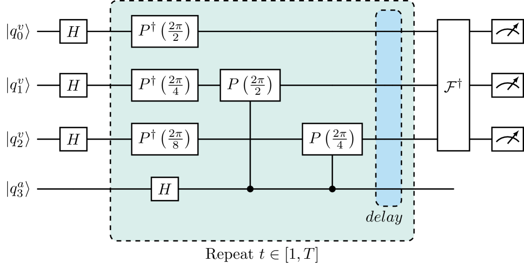
Figure 6: Implementation of discrete time QW on cycle graph using quantum circuits. The $H$ and $P$ are respectively Hadamard and phase gates, and $\mathcal{F}$ is the quantum Fourier transform. The outer shaded block indicates a single time step of the walker and is repeated for $t$ times up to $T$. The inner shaded block modulates the amount of noise in the circuit by a delay operation scaled as in Eq. 8. The final measurements are also shown.

In Fig. 6 we depict the quantum circuit used for the implementation of the QW. At the end of the circuit we collect measurements on the position qubits to obtain the distribution of the walker at every $t\in[1,T]$. The latter is used to define the categorical function from which we draw the new positions of the walker on the graph.

The noise in the circuit is injected with delay operations expressed in seconds by:

$$delay =c\times scaling\times dt,$$ (8)

$$scaling =\left\lfloor\frac{\sin^{2}(\frac{\pi}{2}\frac{t}{T-1})}{8}\right\rfloor 8,$$ (9)

where the value of $scaling$ is truncated to the nearest integer multiple of 8 for hardware reasons, and $dt=5\cdot 10^{-10}$ is the time length in seconds of a single operation on the used devices. The value of $c$ is a coefficient used to guarantee the convergence of the forward process to the uniform distribution within the a priori fixed number of time steps $T=20$, and we choose $c=5\cdot 10^{4}$. This scaling of the injected noise is chosen in analogy to the cosine schedule of noise in the classical DM of Nichols et al. [86]. The backward of the QW-based diffusion model is implemented with a MLP analogous to the one used for the QSW-based case of Section 2.2.

As a proof of concept, we train our model with $6\,903$ full-size $28\times 28$ MNIST images of digits $0$ with the forward implemented in Qiskit [87] initially simulated on fake_brisbane with $10^{5}$ shots and then run on the real device ibm_brisbane with $10^{4}$ shots (the topology is shown in Fig. 7). The number of shots is chosen as the maximum available for the simulator, and reduced considering the computational resources available for the running of the algorithm on the NISQ hardware. This forward protocol is well suited for the used QPU because it has a maximum connectivity degree of 3 and the coin qubit can interact directly with all position qubits. As an additional advantage, it is also possible to run several walkers in parallel on different parts of the same QPU.

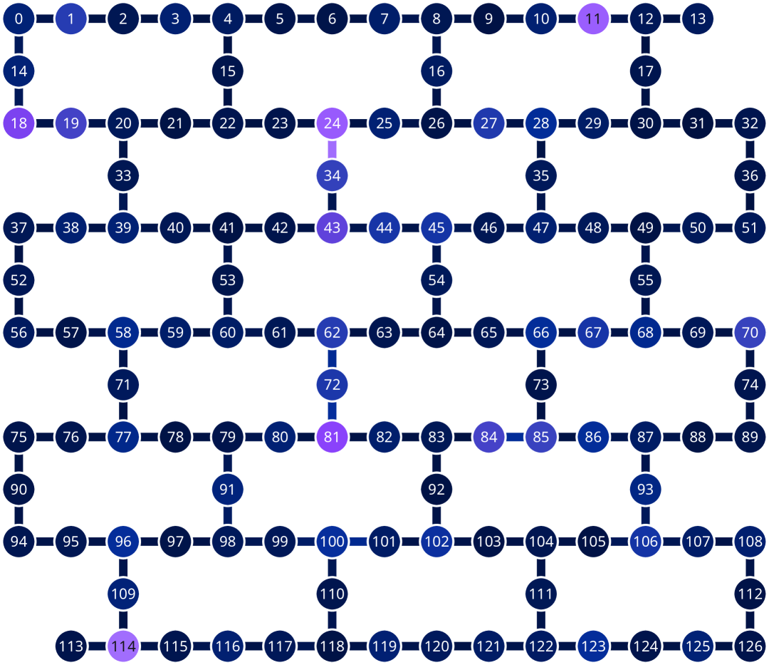
Figure 7: Qubit connectivity map of the real QPU ibm_brisbane (courtesy of IBM [88]). Every circle represents a qubit, and lines represent their connections. Colors code the readout errors (circles) and the errors for the connections (lines). Dark blue indicates a small error, while large one is in purple.

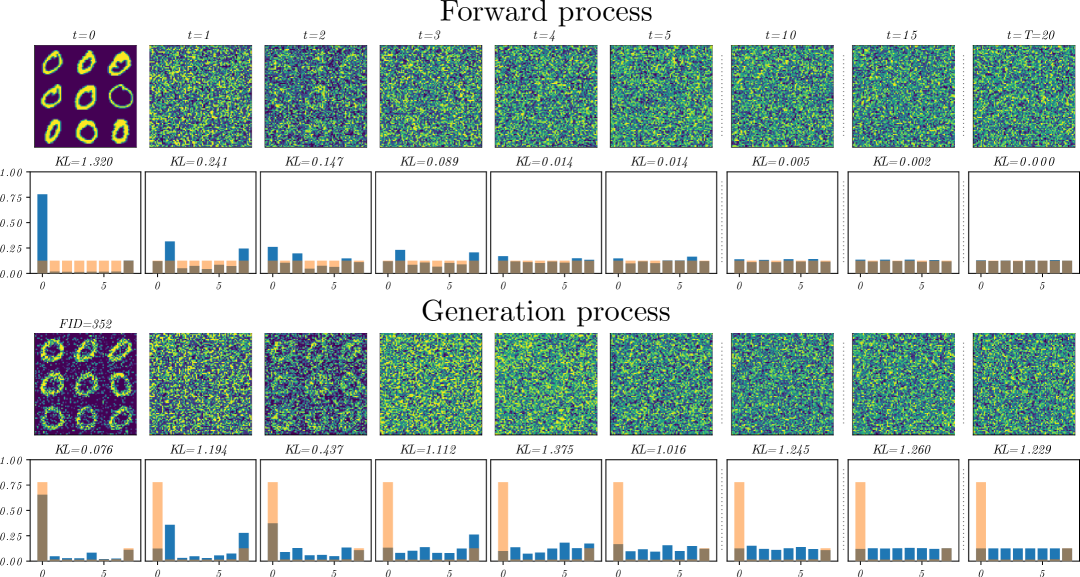
Figure 8: Images generation with QW-based DM with noise from real ibm_brisbane NISQ device. We report for selected values of $t$ the evolution of 9 random samples of the real dataset in forward (first row) and 9 random generated samples in backward (third row). In the second row we show the evolution of the pixel values distributions (orange) for the entire training dataset reporting the KL divergence with the uniform distribution (blue). Finally, in the fourth row we show the value distributions of a generated dataset of the same dimension of the training set comparing it with the original dataset using the KL divergence. Also, we report for $t=0$ the value of FID equal to $352$ between the original and generated dataset.

In Fig. 8 we show the forward and backward processes for image generation implemented on the real IBM machine. The equivalent figure obtained using the simulator is available in the supplementary materials (SM) together with the results on the other digits of MNIST. In the first and third rows are shown, respectively, the quantum forward evolution via QWs (from left to right) and the image generation by a trained classical MLP (from right to left) at different time steps $t$ for 9 samples of the original and generated dataset. In the second row, the transformation of the initial distribution of the pixel values (in blue) for the full training dataset overlaps with the desired final uniform distribution (in orange) with the KL divergence between the two reported on the top. The final row reports the distribution of the pixel values for $6\,903$ generated images (in blue) overlapped with the original distribution of the training dataset (in orange) with the KL divergence between the two on top. In the top distribution at $t=0$ we report the value of FID$=352$ calculated between the original dataset and the equally sized dataset of generated images. Comparing the results of Fig. 5 with Fig. 8, we observe that the latter generates samples with higher values of FID: $114$ (hybrid QSW-based) and $352$ (IBM-based QW). One possible explanation between the simulated results and the real IBM-based ones could be that the underlying dynamics for the evolution of the pixel values is in discrete time for the QWs which are implemented with circuits, while it is in continuous time for QSWs, resulting in a more gradual introduction of noise during the forward process.

3 Discussion and Conclusions

In this work, we show that the impact of quantum noise within the forward DMs dynamics influences the effectiveness of the backward generation process. In particular, we find that a model with a hybrid QSW diffusion dynamics produces sets of samples with a lower FID and is also statistically more solid with respect to its classical counterpart.

Successively, we propose a model that allows one to generate images of any size by harnessing the noise of real NISQ devices taking into account the topology and connectivity of the QPU. More precisely, we generate $28\times 28$ gray-scale MNIST images using only $4$ qubits by efficiently implementing a quantum walk dynamics on a cycle graph whose nodes are the color values of a single image pixel. The invariant property of the graph allows one to independently run the walkers for the single pixels starting from the same initial state and then remapping the outcome to the specific value of the pixel color. Furthermore, our forward protocol enables the implementation of multiple walkers in parallel, requiring a maximum $3$ degree of connectivity between qubits of a QPU. This allows for the implementation on the currently available NISQ devices.

In conclusion, we show how noise can be used as a resource in the context of QGenAI and not only be a detrimental factor for quantum algorithms. Some future research directions can focus on a major integration of the QPU topology with the QW implemented at the circuit level. In particular, we can take more advantages from the connectivity to increase the range of the pixel values, and thus generate high-quality images. Moreover, error correction or mitigation techniques could be used to better control the level of noise of the quantum forward to further improve the capabilities of the backward network. Another interesting outlook can be the possibility of a physical realization of the quantum walk making our model directly applied to quantum data, without performing any quantum embedding in the first stage of the algorithms and then using a quantum ANNs in the reverse process. In conclusion, we believe that the latter can be fruitful where it is necessary to learn unknown quantum phenomena, for instance, in quantum sensing, metrology, chemistry, and biology scenarios.

4 Methods

4.1 Diffusion Models

Diffusion Models (DMs) are a class of latent variable generative models trained to learn the underlying unknown data distribution of a finite dataset in order to generate new similarly distributed synthetic data. The core idea is to use a classical Markov chain to gradually convert an unknown (data) distribution, called posterior, to a simple well-known distribution, e.g. Gaussian or uniform, called prior. The most generic pipeline of DMs is characterized by a forward (or diffusion) and a backward (or denoising) process. In the forward process an initial sample $\mathbf{x}_{0}\sim q(\mathbf{x}_{0})$ is corrupted in a sequence of $T$ increasingly noisy latent variables $\mathbf{x}_{1},\mathbf{x}_{2},\dots,\mathbf{x}_{T}$. Formally, the diffusion process is described by a classical random process via a Markov chain that gradually injects noise on the initial sample $\mathbf{x}_{0}$. More precisely, this is realized by using the Markov transition kernel:

$$q(\mathbf{x}_{t}|\mathbf{x}_{t-1})=K_{\pi}(\mathbf{x}_{t}|\mathbf{x}_{t-1};\beta_{t}),$$ (10)

$$q(\mathbf{x})=\int d\mathbf{x}^{\prime}\ K_{\pi}(\mathbf{x}|\mathbf{x}^{\prime};\beta)q(\mathbf{x}^{\prime}),$$ (11)

where $\beta_{t}\in(0,1)$ is an hyper-parameter at time $t$ of the model (or in physical terms the diffusion rate) describing the level of noise added at each time step, and $\mathbf{x}_{t}$ and $\mathbf{x}_{t-1}$ are the random noisy latent variables at the time steps $t$ and $t-1$, respectively. The scheduling of $\beta_{t}$ is chosen and fixed such that the initial data distribution $q(\mathbf{x}_{0})$ convergences to a well-known stationary distribution $\pi(\mathbf{x}_{T})$ in the limit $T\rightarrow\infty$. The forward trajectory after performing $T$ time steps of diffusion can be written as:

$$q(\mathbf{x}_{0:T})=\prod_{t=1}^{T}q(\mathbf{x}_{t}|\mathbf{x}_{t-1}),$$ (12)

where the chain rule of probability and the Markov property of the process are used to factorize the joint distribution $q(\mathbf{x}_{0:T})$. In addition, in the diffusion process there are no trainable parameters and therefore it does not involve the use of any learning model. The idea of the backward process is to reverse the forward dynamics moving from a pure noise sample $\mathbf{x}_{T}\sim\pi(\mathbf{x}_{T})$ towards a sample of the initial distribution $q(\mathbf{x}_{0})$. The denoising is implemented by an ANN that is trained to learn the reverse trajectory of the diffusion process:

$$p(\mathbf{x}_{T})=\pi(\mathbf{x}_{T})$$ (13)

$$p_{\theta}(\mathbf{x}_{0:T})=p(\mathbf{x}_{T})\prod_{t=1}^{T}p_{\theta}(\mathbf{x}_{t-1}|\mathbf{x}_{t}),$$ (14)

where $p_{\theta}(\mathbf{x}_{t-1}|\mathbf{x}_{t})$ is a parameterized transition kernel having the same functional form of $q(\mathbf{x}_{t}|\mathbf{x}_{t-1})$. A deep ANN, usually with a U-Net architecture [89], is used to estimate the parameters $\theta$ at each time step. The denoising network is trained to optimize the negative log-likelihood on the training data writing the evidence lower bound (ELBO) [90] as follow:

$$\begin{split}L&=D_{\text{KL}}(q(\mathbf{x}_{0:T})||p_{\theta}(\mathbf{x}_{0:T}))\\ &=-\mathbb{E}[\log p_{\theta}(\mathbf{x}_{0:T})]+\text{const}\\ &=\mathbb{E}\Bigg{[}-\log p(\mathbf{x}_{T})-\sum_{t\geq 1}\log\frac{p_{\theta}(\mathbf{x}_{t}|\mathbf{x}_{t-1})}{q(\mathbf{x}_{t}|\mathbf{x}_{t-1})}\Bigg{]}+\text{const}\\ &\geq\mathbb{E}[-\log p_{\theta}(\mathbf{x}_{0})]+\text{const},\end{split}$$ (15)

where the Jensen’s inequality holds in the last line, and the $D_{\text{KL}}(\cdot||\cdot)$ is the KL divergence, which computes the difference between two probability distributions. The objective of the optimization procedure is to minimize the loss function $L$ to reduce the difference between the probability distribution $q(\mathbf{x}_{0})$ and the parameterized distribution $p_{\theta}(\mathbf{x}_{0})$.

4.2 Diffusion models in discrete state-spaces

DMs in discrete state-spaces has been introduced by Sohl-Dickstein et al. for binary random variables [4], and then generalized to categorical random variables characterized by uniform transition probability distribution by Hoogeboom et al. [79]. In the general framework, given a scalar discrete $K$-categories random variable $X$ taking values $x_{t}\in 1,\dots,K$ for $t\in[0,T]$, the forward transition probabilities from the category $i$ to the category $j$ at time $t$ can be realized by matrices:

$$[\mathbf{Q}_{t}]_{i,j}=q(x_{t}=j|x_{t-1}=i).$$ (16)

Denoting the one-hot version of $x$ with the row vector $\mathbf{x}$, i.e. a vector whose elements for the category $k$ are $x_{k}=1$ and $x_{j}=0$ for $j\not=k$, forward transition kernel can be written as:

$$q(\mathbf{x}_{t}|\mathbf{x}_{t-1})=\text{Cat}(\mathbf{x}_{t};\mathbf{p}=\mathbf{x}_{t-1}\mathbf{Q}_{t}),$$ (17)

where Cat$(\mathbf{x};\mathbf{p})$ is the categorical distribution over the one-hot row vector $\mathbf{x}$ with probability $\mathbf{p}$. Starting from an initial data $\mathbf{x}_{0}$, the data $\mathbf{x}_{t}$ after $t$ time steps can be sampled from the transition kernel:

$$\mathbf{x}_{t} \sim q(\mathbf{x}_{t}|\mathbf{x}_{0}),$$ (18)

$$q(\mathbf{x}_{t}|\mathbf{x}_{0}) =\text{Cat}(\mathbf{x}_{t};\mathbf{p}=\mathbf{x}_{0}\bar{\mathbf{Q}}_{t}),$$ (19)

where $\bar{\mathbf{Q}}_{t}:=\mathbf{Q}_{1}\mathbf{Q}_{2}\dots\mathbf{Q}_{t}$ is the cumulative product of the transition matrices. The rows of the matrix $\bar{\mathbf{Q}}_{t}$ must satisfy two constraints: i) must sum to one to conserve the probability mass, and ii) must converge to a known stationary distribution in the limit $t\rightarrow\infty$. Moreover, it can be shown [79, 12] that a closed-form of the categorical posterior $q(\mathbf{x}_{t-1}|\mathbf{x}_{t},\mathbf{x}_{0})$ can be computed:

$$q(\mathbf{x}_{t-1}|\mathbf{x}_{t},\mathbf{x}_{0})=\dfrac{q(\mathbf{x}_{t}|\mathbf{x}_{t-1},\mathbf{x}_{0})q(\mathbf{x}_{t-1}|\mathbf{x}_{0})}{q(\mathbf{x}_{t}|\mathbf{x}_{0})},$$ (20)

where $q(\mathbf{x}_{t}|\mathbf{x}_{t-1},\mathbf{x}_{0})=q(\mathbf{x}_{t}|\mathbf{x}_{t-1})$ due to the Markov property and all the terms can be calculated from Eqs. 17 and 19. The denoising process is implemented via an ANN predicting the logits of the parameterized distribution:

$$p_{\theta}(\mathbf{x}_{t-1}|\mathbf{x}_{t}),$$ (21)

which has the functional form of a categorical distribution [79, 12]. The optimization is realized by minimize the loss function:

$$L=D_{\text{KL}}(q(\mathbf{x}_{t-1}|\mathbf{x}_{t},\mathbf{x}_{0})||p_{\theta}(\mathbf{x}_{t-1}|\mathbf{x}_{t})).$$ (22)

4.3 Classical Random Walk on Graph

A graph is a pair $G=(V,E)$, where $V$ is a finite and non-empty set whose elements $v_{i}$, $i=1,\dots\absolutevalue{V}$, are called vertices (or nodes), and $E$ is a non-empty set of unordered pairs of vertices $e_{ij}=\{v_{i},v_{j}\}$, called edges (or links). The order and the size of a graph are the cardinality $\absolutevalue{V}$ and $\absolutevalue{E}$ of the sets $V$ and $E$, respectively. The number $d_{v}$ of edges connected to the vertex $v$ is called degree of the vertex. A graph is called undirected if the edges of the graph do not have a direction, or directed otherwise. A graph is completely defined by its adjacency matrix $A$ that contains information on the topology of the graph, and whose element are defined as follow:

$$[A]_{i,j}=\begin{cases}1,&\text{if}\quad e_{ij}\in E.\\ 0,&\text{if}\quad e_{ij}\not\in E.\end{cases}$$ (23)

In a discrete-time CRW on an undirected graph $G$, at each step $t\in\mathbb{N}$ a walker jumps between two connected nodes $v_{i},v_{j}$ with some probability that is described by the stochastic transition matrix $S=[S]_{i,j}$ [91, 92, 36]. $S$ is related to the adjacency matrix by the equation: $[S]_{i,j}=[A]_{i,j}/d_{i}$. Formally, a walker is represented by a discrete random variable $X$ and its trajectory after the $T$ time steps is the set $\{x_{1},\dots,x_{T}\}$, where the value $x_{t}$, with $t=1,\dots,T$, corresponds to the node occupied by the walker at time $t$. A CRW is a Markov process, that is, the distribution at time $t+1$ depends only on the distribution at time $t$. Given $\mathbf{p}_{t}=\{p_{i}^{(t)}\}$ the occupation probability distribution of a walker over the nodes $v_{i}$ after $t$ time steps, the evolution of the distribution at time $t+1$ is given by:

$$\mathbf{p}_{t+1}=S\mathbf{p}_{t}.$$ (24)

The distribution of a CRW converges to a limiting stationary solution:

$$\pi=\Bigg{\{}\dfrac{d_{i}}{2\absolutevalue{V}}\Bigg{\}},\quad t\rightarrow\infty,$$ (25)

independently of the initial distribution $\mathbf{p}_{0}$. For a $d-$regular graph (all vertices have the same degree $d$) the limiting stationary distribution is uniform over the nodes of the graph.

4.4 Quantum Walks

In quantum information theory, Quantum Walks were introduced by Aharonov et al. [32] as quantum analogues of classical random walks. However, in CRWs the dynamics is purely stochastic at each time step, while QWs evolve via a deterministic dynamics, and the stochasticity comes out only when a measurement is performed on the quantum state of the walker  [32, 93]. Moreover, QWs involve peculiar quantum mechanical properties such as coherent superposition, entanglement, and quantum interference, resulting in a faster spread (ballistic for the quantum case, while diffusive for the classical one). There exist two different formulations of QWs: i) Continuous-time Quantum Walks and ii) Discrete-time Quantum Walks. In the former, the unitary evolution operator can be applied at any time $t$, while in the latter, the operator can be applied only in discrete time steps. Furthermore, DTQWs need an extra degree of freedom, called “coin”, which stores directions and speeds up the dynamics of the walker [34].

4.4.1 Discrete-Time Quantum Walks on Graph

Given a graph $G(V,E)$, let $\mathcal{H}_{V}$ be the Hilbert space spanned by the position states $\{\ket{v}:v=1,\dots,\absolutevalue{V}\}$, and let $\mathcal{H}_{A}$ be an auxiliary Hilbert space spanned by the coin states $\{\ket{\downarrow},\ket{\uparrow}\}$. The total Hilbert space $\mathcal{H}$ associated to a QW is obtained by the tensor product between the auxiliary space and the position space:

$$\mathcal{H}=\mathcal{H}_{A}\otimes\mathcal{H}_{V}.$$ (26)

In general, a state is written as:

$$\ket{\psi}=\ket{a}\otimes\ket{v},\quad\ket{a}\in\mathcal{H}_{A}\quad\ket{v}\in\mathcal{H}_{V}.$$ (27)

The dynamics of the quantum walker is governed by the unitary single time-step operator $\hat{U}$ acting on the total Hilbert space:

$$\hat{U}=\hat{S}\cdot(\hat{C}\otimes\hat{I}),$$ (28)

where $\hat{I}$ is the identity on position space, $\hat{C}$ is the coin operator acting on the auxiliary space, and $\hat{S}$ is shift operator acting only on position space and moving the walker from state $\ket{v}$ to state $\ket{v+1}$, or $\ket{v-1}$. Formally, the shift operator is given by:

$$\hat{S}=\sum_{v}\outerproduct{\uparrow}{\uparrow}\otimes\outerproduct{v+1}{v}+\outerproduct{\downarrow}{\downarrow}\otimes\outerproduct{v-1}{v}.$$ (29)

The coin operator $\hat{C}$ can be chosen in the family of unitary operators and its choice leads to symmetric (unbiased walk) or asymmetric (biased walk) distributions. A common choices for $\hat{C}$ is the Hadamard coin:

$$\hat{H}=\frac{1}{2}\left(\begin{array}[]{cc}1&1\\ 1&-1\end{array}\right),$$ (30)

which leads to an unbiased walk. The state of a quantum walk after $t$ discrete time steps is given by:

$$\ket{\psi(t)}=\hat{U}^{\otimes t}\ket{\psi(0)}.$$ (31)

In general, QWs do not converge to any limiting distribution in contrast to the classical ones: the limit $\lim_{t\to\infty}\ket{\psi(t)}$ does not exist due to the unitary evolution [94]. Moreover, the interference effects lead a quantum walker to spread quadratically faster with respect to its classical counterpart. Namely, in the classical case after $t$ time steps the expected distance from the origin is of order $\sigma\sim\sqrt{t}$, while in the quantum case it is of order $\sigma\sim t$, as shown in Fig. 9

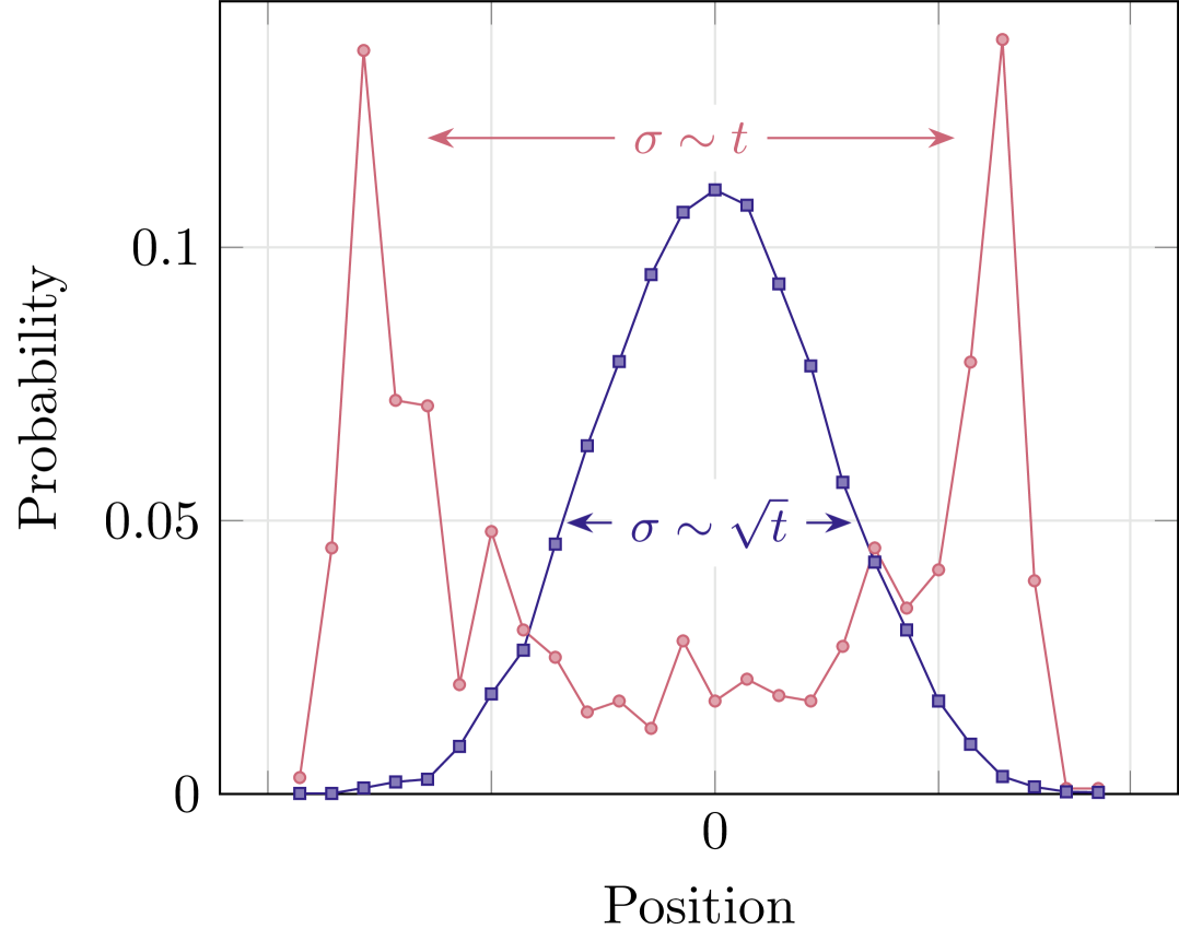
Figure 9: Comparison between the Gaussian probability distribution (violet squares) obtained from a CRW and probability distribution of a QW with Hadamard coin (red circles).

4.5 Numerical and Real Implementation

The implementation is carried out in Python 3 using Qiskit [95], an IBM open-source software to work with real quantum processors at the circuit level, QuTiP [96], an open-source computational physics software to simulate open quantum systems dynamics, and PyTorch [97], which is a flexible and efficient machine and deep learning library. For the implementations of DMs via QSWs on a cycle graph, we used the QuTip function mesolve to compute the evolution of the state $\rho_{t}$ of the quantum stochastic walker in Eq. 4 for different values of $\omega$ and fixing $\delta t=6\cdot 10^{-1}$. Regarding the forward process with QWs in Section 2.3, we use the Qiskit library to implement the QWs dynamics both simulated and on real IBM QPU. The backward process is implemented via MLPs of PyTorch linear layers with Rectified Linear Unit (ReLU) activation functions. More precisely, the architecture is structured with a head layer of size $800$ shared between all time steps $t$ and two tail layers of the same size specialized for each step. The input layer takes the one-hot encoding of all the positions of the walkers at the time step $t$ for all the image pixels, and the final layer predicts their logits at the previous time $t-1$. In optimization, the categorical cross-entropy loss is minimized for $10^{4}$ epochs using Adam [98] with a batch size of 16 samples and setting the learning rate equal to $10^{-3}$.

Author Contributions

M.P. and S.M. performed the implementation and experiments. M.P., S.M., F.A.V. and F.C. discussed and analyzed the results. M.P., S.M., F.C. conceived the methodology, while F.C. proposed and supervised the project. M.P., S.M. and F.A.V. wrote the original Draft. M.P., S.M., F.A.V. and F.C. performed the review and Editing.

Competing Interests

The authors declare no competing interests.

See pages - of supplementary.pdf

References

- \bibcommenthead
- Goodfellow et al. [2020] Goodfellow, I., Pouget-Abadie, J., Mirza, M., Xu, B., Warde-Farley, D., Ozair, S., Courville, A., Bengio, Y.: Generative adversarial networks. Communications of the ACM 63(11), 139–144 (2020)
- Kingma and Welling [2019] Kingma, D.P., Welling, M.: An introduction to variational autoencoders. Foundations and Trends® in Machine Learning 12(4), 307–392 (2019)
- Rezende and Mohamed [2015] Rezende, D., Mohamed, S.: Variational inference with normalizing flows. In: Bach, F., Blei, D. (eds.) Proceedings of the 32nd International Conference on Machine Learning. Proceedings of Machine Learning Research, vol. 37, pp. 1530–1538. PMLR, Lille, France (2015)
- Sohl-Dickstein et al. [2015] Sohl-Dickstein, J., Weiss, E., Maheswaranathan, N., Ganguli, S.: Deep unsupervised learning using nonequilibrium thermodynamics. In: Bach, F., Blei, D. (eds.) Proceedings of the 32nd International Conference on Machine Learning. Proceedings of Machine Learning Research, vol. 37, pp. 2256–2265. PMLR, Lille, France (2015)
- Ho et al. [2020] Ho, J., Jain, A., Abbeel, P.: Denoising diffusion probabilistic models. In: Larochelle, H., Ranzato, M., Hadsell, R., Balcan, M.F., Lin, H. (eds.) Advances in Neural Information Processing Systems, vol. 33, pp. 6840–6851 (2020)
- Paiano et al. [2024] Paiano, M., Martina, S., Giannelli, C., Caruso, F.: Transfer learning with generative models for object detection on limited datasets. Machine Learning: Science and Technology 5(3), 035041 (2024)
- Dhariwal and Nichol [2021] Dhariwal, P., Nichol, A.: Diffusion models beat gans on image synthesis. In: Ranzato, M., Beygelzimer, A., Dauphin, Y., Liang, P.S., Vaughan, J.W. (eds.) Advances in Neural Information Processing Systems, vol. 34, pp. 8780–8794 (2021)
- Kong et al. [2021] Kong, Z., Ping, W., Huang, J., Zhao, K., Catanzaro, B.: Diffwave: A versatile diffusion model for audio synthesis. In: International Conference on Learning Representations (2021)
- Saharia et al. [2022] Saharia, C., Chan, W., Saxena, S., Li, L., Whang, J., Denton, E.L., Ghasemipour, K., Gontijo Lopes, R., Karagol Ayan, B., Salimans, T., et al.: Photorealistic text-to-image diffusion models with deep language understanding. Advances in Neural Information Processing Systems 35, 36479–36494 (2022)
- Rombach et al. [2022] Rombach, R., Blattmann, A., Lorenz, D., Esser, P., Ommer, B.: High-resolution image synthesis with latent diffusion models. In: Proceedings of the IEEE/CVF Conference on Computer Vision and Pattern Recognition (CVPR), pp. 10684–10695 (2022)
- Lugmayr et al. [2022] Lugmayr, A., Danelljan, M., Romero, A., Yu, F., Timofte, R., Van Gool, L.: Repaint: Inpainting using denoising diffusion probabilistic models. In: Proceedings of the IEEE/CVF Conference on Computer Vision and Pattern Recognition (CVPR), pp. 11461–11471 (2022)
- [12] Austin, J., Johnson, D.D., Ho, J., Tarlow, D., Berg, R.: Structured denoising diffusion models in discrete state-spaces. In: Ranzato, M., Beygelzimer, A., Dauphin, Y., Liang, P.S., Vaughan, J.W. (eds.) Advances in Neural Information Processing Systems, vol. 34, pp. 17981–17993. Curran Associates, Inc. (2021)
- [13] Tashiro, Y., Song, J., Song, Y., Ermon, S.: Csdi: Conditional score-based diffusion models for probabilistic time series imputation. In: Ranzato, M., Beygelzimer, A., Dauphin, Y., Liang, P.S., Vaughan, J.W. (eds.) Advances in Neural Information Processing Systems, vol. 34, pp. 24804–24816. Curran Associates, Inc. (2021)
- [14] Stable Diffusion. https://stability.ai/stable-image
- [15] DALL- E4. https://dalle4ai.com
- Shor [1994] Shor, P.W.: Algorithms for quantum computation: discrete logarithms and factoring. In: Proceedings 35th Annual Symposium on Foundations of Computer Science, pp. 124–134. IEEE Computer Society, USA (1994)
- Shor [1997] Shor, P.W.: Polynomial-time algorithms for prime factorization and discrete logarithms on a quantum computer. SIAM J. Comput. 26(5), 1484–1509 (1997)
- Grover [1996] Grover, L.K.: A fast quantum mechanical algorithm for database search. In: Proceedings of the Twenty-Eighth Annual ACM Symposium on Theory of Computing. STOC ’96, pp. 212–219. Association for Computing Machinery, New York, NY, USA (1996)
- Georgescu et al. [2014] Georgescu, I.M., Ashhab, S., Nori, F.: Quantum simulation. Rev. Mod. Phys. 86, 153–185 (2014)
- O’Malley et al. [2016] O’Malley, P.J.J., Babbush, R., Kivlichan, I.D., Romero, J., McClean, J.R., Barends, R., Kelly, J., Roushan, P., Tranter, A., Ding, N., Campbell, B., Chen, Y., Chen, Z., Chiaro, B., Dunsworth, A., Fowler, A.G., Jeffrey, E., Lucero, E., Megrant, A., Mutus, J.Y., Neeley, M., Neill, C., Quintana, C., Sank, D., Vainsencher, A., Wenner, J., White, T.C., Coveney, P.V., Love, P.J., Neven, H., Aspuru-Guzik, A., Martinis, J.M.: Scalable quantum simulation of molecular energies. Phys. Rev. X 6, 031007 (2016)
- Babbush et al. [2018] Babbush, R., Wiebe, N., McClean, J., McClain, J., Neven, H., Chan, G.K.-L.: Low-depth quantum simulation of materials. Phys. Rev. X 8, 011044 (2018)
- Harrow et al. [2009] Harrow, A.W., Hassidim, A., Lloyd, S.: Quantum algorithm for linear systems of equations. Phys. Rev. Lett. 103, 150502 (2009)
- Crosson and Harrow [2016] Crosson, E., Harrow, A.W.: Simulated quantum annealing can be exponentially faster than classical simulated annealing. In: 2016 IEEE 57th Annual Symposium on Foundations of Computer Science (FOCS), pp. 714–723 (2016)
- Farhi and Harrow [2019] Farhi, E., Harrow, A.W.: Quantum Supremacy through the Quantum Approximate Optimization Algorithm (2019)
- [25] Preskill, J.: Fault-tolerant quantum computation. In: Introduction to Quantum Computation and Information, pp. 213–269. World Scientific (1998)
- Preskill [2018] Preskill, J.: Quantum Computing in the NISQ era and beyond. Quantum 2, 79 (2018)
- [27] IBM Quantum Prcessing Unit. https://www.ibm.com/think/topics/qpu
- [28] QuEra. https://www.quera.com/glossary/processing-unit
- Knill and Laflamme [1997] Knill, E., Laflamme, R.: Theory of quantum error-correcting codes. Phys. Rev. A 55, 900–911 (1997)
- Campbell [2024] Campbell, E.: A series of fast-paced advances in quantum error correction. Nature Reviews Physics 6(3), 160–161 (2024)
- AI and Collaborators [2024] AI, G.Q., Collaborators: Quantum error correction below the surface code threshold. Nature (2024)
- Aharonov et al. [1993] Aharonov, Y., Davidovich, L., Zagury, N.: Quantum random walks. Phys. Rev. A 48, 1687–1690 (1993)
- Childs and Goldstone [2004] Childs, A.M., Goldstone, J.: Spatial search by quantum walk. Phys. Rev. A 70, 022314 (2004)
- Ambainis et al. [2005] Ambainis, A., Kempe, J., Rivosh, A.: Coins make quantum walks faster. In: Proceedings of the Sixteenth Annual ACM-SIAM Symposium on Discrete Algorithms. SODA ’05, pp. 1099–1108. Society for Industrial and Applied Mathematics, USA (2005)
- Magniez et al. [2011] Magniez, F., Nayak, A., Roland, J., Santha, M.: Search via quantum walk. SIAM Journal on Computing 40(1), 142–164 (2011)
- Caruso [2014] Caruso, F.: Universally optimal noisy quantum walks on complex networks. New Journal of Physics 16(5), 055015 (2014)
- Caruso et al. [2016] Caruso, F., Crespi, A., Ciriolo, A.G., Sciarrino, F., Osellame, R.: Fast escape of a quantum walker from an integrated photonic maze. Nature Communications 7(1), 11682 (2016)
- Dalla Pozza et al. [2022] Dalla Pozza, N., Buffoni, L., Martina, S., Caruso, F.: Quantum reinforcement learning: the maze problem. Quantum Machine Intelligence 4(1), 11 (2022)
- Abd El-Latif et al. [2020] Abd El-Latif, A.A., Abd-El-Atty, B., Amin, M., Iliyasu, A.M.: Quantum-inspired cascaded discrete-time quantum walks with induced chaotic dynamics and cryptographic applications. Scientific Reports 10(1), 1930 (2020)
- Zeuner et al. [2021] Zeuner, J., Pitsios, I., Tan, S.-H., Sharma, A.N., Fitzsimons, J.F., Osellame, R., Walther, P.: Experimental quantum homomorphic encryption. npj Quantum Information 7(1), 25 (2021)
- Kasture et al. [2025] Kasture, S., Acheche, S., Henriet, L., Henry, L.-P.: Multiparticle quantum walks for distinguishing hard graphs (2025)
- Lovett et al. [2010] Lovett, N.B., Cooper, S., Everitt, M., Trevers, M., Kendon, V.: Universal quantum computation using the discrete-time quantum walk. Phys. Rev. A 81, 042330 (2010)
- Singh et al. [2021] Singh, S., Chawla, P., Sarkar, A., Chandrashekar, C.M.: Universal quantum computing using single-particle discrete-time quantum walk. Scientific Reports 11(1), 11551 (2021)
- Chawla et al. [2023] Chawla, P., Singh, S., Agarwal, A., Srinivasan, S., Chandrashekar, C.M.: Multi-qubit quantum computing using discrete-time quantum walks on closed graphs. Scientific Reports 13(1), 12078 (2023)
- Dür et al. [2002] Dür, W., Raussendorf, R., Kendon, V.M., Briegel, H.-J.: Quantum walks in optical lattices. Phys. Rev. A 66, 052319 (2002)
- Schreiber et al. [2012] Schreiber, A., Gábris, A., Rohde, P.P., Laiho, K., Štefaňák, M., Potoček, V., Hamilton, C., Jex, I., Silberhorn, C.: A 2d quantum walk simulation of two-particle dynamics. Science 336(6077), 55–58 (2012)
- Goyal et al. [2013] Goyal, S.K., Roux, F.S., Forbes, A., Konrad, T.: Implementing quantum walks using orbital angular momentum of classical light. Phys. Rev. Lett. 110, 263602 (2013)
- Lahini et al. [2018] Lahini, Y., Steinbrecher, G.R., Bookatz, A.D., Englund, D.: Quantum logic using correlated one-dimensional quantum walks. npj Quantum Information 4(1), 2 (2018)
- Acasiete et al. [2020] Acasiete, F., Agostini, F.P., Moqadam, J.K., Portugal, R.: Implementation of quantum walks on ibm quantum computers. Quantum Information Processing 19(12), 426 (2020)
- Razzoli et al. [2024] Razzoli, L., Cenedese, G., Bondani, M., Benenti, G.: Efficient implementation of discrete-time quantum walks on quantum computers. Entropy 26(4) (2024)
- Whitfield et al. [2010] Whitfield, J.D., Rodríguez-Rosario, C.A., Aspuru-Guzik, A.: Quantum stochastic walks: A generalization of classical random walks and quantum walks. Physical Review A—Atomic, Molecular, and Optical Physics 81(2), 022323 (2010)
- [52] Wittek, P.: Quantum machine learning: what quantum computing means to data mining. Academic Press (2014)
- Biamonte et al. [2017] Biamonte, J., Wittek, P., Pancotti, N., Rebentrost, P., Wiebe, N., Lloyd, S.: Quantum machine learning. Nature 549(7671), 195–202 (2017)
- Schuld and Petruccione [2021] Schuld, M., Petruccione, F.: Machine Learning with Quantum Computers. Springer, (2021)
- McClean et al. [2016] McClean, J.R., Romero, J., Babbush, R., Aspuru-Guzik, A.: The theory of variational hybrid quantum-classical algorithms. New Journal of Physics 18(2), 023023 (2016)
- Bharti et al. [2022] Bharti, K., Cervera-Lierta, A., Kyaw, T.H., Haug, T., Alperin-Lea, S., Anand, A., Degroote, M., Heimonen, H., Kottmann, J.S., Menke, T., Mok, W.-K., Sim, S., Kwek, L.-C., Aspuru-Guzik, A.: Noisy intermediate-scale quantum algorithms. Rev. Mod. Phys. 94, 015004 (2022)
- Das et al. [2023] Das, S., Zhang, J., Martina, S., Suter, D., Caruso, F.: Quantum pattern recognition on real quantum processing units. Quantum Machine Intelligence 5(1), 16 (2023)
- Geng et al. [2022] Geng, A., Moghiseh, A., Redenbach, C., Schladitz, K.: A hybrid quantum image edge detector for the nisq era. Quantum Machine Intelligence 4(2), 15 (2022)
- Peruzzo et al. [2014] Peruzzo, A., McClean, J., Shadbolt, P., Yung, M.-H., Zhou, X.-Q., Love, P.J., Aspuru-Guzik, A., O’Brien, J.L.: A variational eigenvalue solver on a photonic quantum processor. Nature Communications 5(1), 4213 (2014)
- Kandala et al. [2017] Kandala, A., Mezzacapo, A., Temme, K., Takita, M., Brink, M., Chow, J.M., Gambetta, J.M.: Hardware-efficient variational quantum eigensolver for small molecules and quantum magnets. Nature 549(7671), 242–246 (2017)
- González-García et al. [2022] González-García, G., Trivedi, R., Cirac, J.I.: Error propagation in nisq devices for solving classical optimization problems. PRX Quantum 3, 040326 (2022)
- Zhang et al. [2021] Zhang, K., Rao, P., Yu, K., Lim, H., Korepin, V.: Implementation of efficient quantum search algorithms on nisq computers. Quantum Information Processing 20(7), 233 (2021)
- Farhi and Neven [2018] Farhi, E., Neven, H.: Classification with Quantum Neural Networks on Near Term Processors (2018)
- Lloyd and Weedbrook [2018] Lloyd, S., Weedbrook, C.: Quantum generative adversarial learning. Phys. Rev. Lett. 121, 040502 (2018)
- Dallaire-Demers and Killoran [2018] Dallaire-Demers, P.-L., Killoran, N.: Quantum generative adversarial networks. Phys. Rev. A 98, 012324 (2018)
- Khoshaman et al. [2018] Khoshaman, A., Vinci, W., Denis, B., Andriyash, E., Sadeghi, H., Amin, M.H.: Quantum variational autoencoder. Quantum Science and Technology 4(1), 014001 (2018)
- Parigi et al. [2024] Parigi, M., Martina, S., Caruso, F.: Quantum-noise-driven generative diffusion models. Advanced Quantum Technologies, 2300401 (2024)
- Ma et al. [2024] Ma, H., Ye, L., Guo, X., Ruan, F., Zhao, Z., Li, M., Wang, Y., Yang, J.: Quantum generative adversarial networks in a silicon photonic chip with maximum expressibility. Advanced Quantum Technologies, 2400171 (2024)
- Hibat-Allah et al. [2024] Hibat-Allah, M., Mauri, M., Carrasquilla, J., Perdomo-Ortiz, A.: A framework for demonstrating practical quantum advantage: comparing quantum against classical generative models. Communications Physics 7(1), 68 (2024)
- Kölle et al. [2024] Kölle, M., Stenzel, G., Stein, J., Zielinski, S., Ommer, B., Linnhoff-Popien, C.: Quantum Denoising Diffusion Models (2024)
- DeFalco et al. [2024] DeFalco, F., Ceschini, A., Sebastianelli, A., LeSaux, B., Panella, M.: Quantum latent diffusion models. Quantum Machine Intelligence 6(2), 85 (2024)
- Cacioppo et al. [2024] Cacioppo, A., Colantonio, L., Bordoni, S., Giagu, S.: Quantum diffusion models for quantum data learning in high-energy physics. QTML 2024 Conference (2024)
- De Falco et al. [2024] De Falco, F., Ceschini, A., Sebastianelli, A., Le Saux, B., Panella, M.: Quantum hybrid diffusion models for image synthesis. KI - Künstliche Intelligenz (2024)
- Kivijervi [2024] Kivijervi, N.T.: Quantum diffusion model. Master’s thesis, University of Oslo (2024)
- Zhang et al. [2024] Zhang, B., Xu, P., Chen, X., Zhuang, Q.: Generative quantum machine learning via denoising diffusion probabilistic models. Phys. Rev. Lett. 132, 100602 (2024)
- Chen et al. [2024] Chen, C., Zhao, Q., Zhou, M., He, Z., Sun, Z., Situ, H.: Quantum Generative Diffusion Model: A Fully Quantum-Mechanical Model for Generating Quantum State Ensemble (2024)
- Cacioppo et al. [2023] Cacioppo, A., Colantonio, L., Bordoni, S., Giagu, S.: Quantum Diffusion Models (2023)
- Kwun et al. [2024] Kwun, G., Zhang, B., Zhuang, Q.: Mixed-State Quantum Denoising Diffusion Probabilistic Model (2024)
- [79] Hoogeboom, E., Nielsen, D., Jaini, P., Forré, P., Welling, M.: Argmax flows and multinomial diffusion: Learning categorical distributions. In: Ranzato, M., Beygelzimer, A., Dauphin, Y., Liang, P.S., Vaughan, J.W. (eds.) Advances in Neural Information Processing Systems, vol. 34, pp. 12454–12465. Curran Associates, Inc. (2021)
- Kossakowski [1972] Kossakowski, A.: On quantum statistical mechanics of non-hamiltonian systems. Reports on Mathematical Physics 3(4), 247–274 (1972)
- Lindblad [1976] Lindblad, G.: On the generators of quantum dynamical semigroups. Communications in Mathematical Physics 48(2), 119–130 (1976)
- Gorini et al. [1976] Gorini, V., Kossakowski, A., Sudarshan, E.C.G.: Completely positive dynamical semigroups of n‐level systems. Journal of Mathematical Physics 17(5), 821–825 (1976)
- LeCun et al. [2010] LeCun, Y., Cortes, C., Burges, C.: Mnist handwritten digit database. ATT Labs [Online]. Available: http://yann.lecun.com/exdb/mnist 2 (2010)
- Szegedy et al. [2016] Szegedy, C., Vanhoucke, V., Ioffe, S., Shlens, J., Wojna, Z.: Rethinking the inception architecture for computer vision. In: Proceedings of the IEEE Conference on Computer Vision and Pattern Recognition (CVPR), pp. 2818–2826 (2016)
- Krzywinski and Altman [2014] Krzywinski, M., Altman, N.: Visualizing samples with box plots. Nature Methods 11(2), 119–120 (2014)
- [86] Nichol, A.Q., Dhariwal, P.: Improved denoising diffusion probabilistic models. In: Meila, M., Zhang, T. (eds.) Proceedings of the 38th International Conference on Machine Learning, ICML 2021, 18-24 July 2021, Virtual Event. Proceedings of Machine Learning Research, vol. 139, pp. 8162–8171. PMLR (2021)
- Javadi-Abhari et al. [2024] Javadi-Abhari, A., Treinish, M., Krsulich, K., Wood, C.J., Lishman, J., Gacon, J., Martiel, S., Nation, P.D., Bishop, L.S., Cross, A.W., Johnson, B.R., Gambetta, J.M.: Quantum computing with Qiskit (2024)
- [88] IBM Quantum Computing. https://www.ibm.com/quantum
- Ronneberger et al. [2015] Ronneberger, O., Fischer, P., Brox, T.: U-net: Convolutional networks for biomedical image segmentation. In: Navab, N., Hornegger, J., Wells, W.M., Frangi, A.F. (eds.) Medical Image Computing and Computer-Assisted Intervention – MICCAI 2015, pp. 234–241. Springer, Cham (2015)
- Kingma and Welling [2014] Kingma, D.P., Welling, M.: Auto-Encoding Variational Bayes. In: 2nd International Conference on Learning Representations, ICLR 2014, Banff, AB, Canada, April 14-16, 2014, Conference Track Proceedings (2014)
- [91] Weiss, G.H., Rubin, R.J.: Random Walks: Theory and Selected Applications, pp. 363–505. John Wiley & Sons, Ltd (1982)
- [92] Weiss, G.H.: Aspects and Applications of the Random Walk International Congress Series Random Materials and Processes, ISSN 0925-5850. North-Holland (1994)
- Kempe [2009] Kempe, J.: Quantum random walks: an introductory overview. Contemporary Physics 50(1), 339–359 (2009)
- Aharonov et al. [2001] Aharonov, D., Ambainis, A., Kempe, J., Vazirani, U.: Quantum walks on graphs. In: Proceedings of the Thirty-Third Annual ACM Symposium on Theory of Computing. STOC ’01, pp. 50–59. Association for Computing Machinery, New York, NY, USA (2001)
- [95] IBM Qiskit. https://www.ibm.com/quantum/qiskit
- [96] QuTip. https://qutip.org
- [97] PyTorch. https://pytorch.org
- Kingma and Ba [2017] Kingma, D.P., Ba, J.: Adam: A method for stochastic optimization. e-print arXiv:1412.6980 (2017)