Algorithm Unrolling-based Denoising of Multimodal Graph Signals

Abstract

We propose a denoising method of multimodal graph signals by iteratively solving signal restoration and graph learning problems. Many complex-structured data, i.e., those on sensor networks, can capture multiple modalities at each measurement point, referred to as modalities. They are also assumed to have an underlying structure or correlations in modality as well as space. Such multimodal data are regarded as graph signals on a twofold graph and they are often corrupted by noise. Furthermore, their spatial/modality relationships are not always given a priori: We need to estimate twofold graphs during a denoising algorithm. In this paper, we consider a signal denoising method on twofold graphs, where graphs are learned simultaneously. We formulate an optimization problem for that and parameters in an iterative algorithm are learned from training data by unrolling the iteration with deep algorithm unrolling. Experimental results on synthetic and real-world data demonstrate that the proposed method outperforms existing model- and deep learning-based graph signal denoising methods.

I INTRODUCTION

Sensor networks have been extensively utilized in various applications including environmental monitoring, Internet of Things (IoT), and home automation systems [2, 3, 4, 5, 6]. Observed signals on sensor networks often corrupted by noise which affect to performances for the following applications. Therefore, denoising is a fundamental task for sensor network-based signal processing systems [7, 8].

Networks are mathematically represented by graphs and signals on a network are called graph signals. Graph signal processing (GSP) includes theory and algorithms to analyze graph signals [9, 10, 11]. GSP mainly considers spatially distributed signal values whose domain is represented as nodes of a spatial graph.

In sensor networks, however, we also encounter relationships among modalities since sensors often collect multiple features like temperature and humidity. Some modalities are strongly correlated and the others are not. This can be represented as a modality graph. It is visualized in Fig. 1. As a result, we can assume many sensor network data can be viewed as signals lying on a twofold graph [12].

There are three main types of approaches to graph signal restoration: 1) model-based approach, 2) data-driven approach, and 3) hybrid approach.

The model-based approach designs a regularized objective function based on the prior for the observed data and finds its minimum solution. The smoothness prior in the node and/or graph frequency domains is widely used for graph signals [13, 14, 15, 16, 17, 18]. The problem is often solved with iterative algorithms. Note that the model-based method usually needs to tune hyperparameters, such as the step size of the iterative algorithm and the regularization strength. They are fixed throughout the iterative process and in many cases, they are manually tuned.

The data-driven approach learns (hyper)parameters from given training data with machine learning techniques. The current majority is based on graph neural networks (GNNs). The representative example is graph convolutional networks (GCNs) [19]. However, GNNs do not always outperform model-based methods for signal restoration [20]. This may stem from the fact that, in contrast to uniformly sampled signals like image and audio signals, deep layers for GNNs may not result in good performance [21, 22]. We also encounter a challenge for training data: We need to collect enough number of data for training, but this is not often the case for the graph setting.

The hybrid approach has been proposed to overcome the aforementioned challenges in the model- and data-driven methods. This often integrates (sometimes black-box) denoisers in an iterative algorithm [15]. In terms of the hyperparameter tuning, deep algorithm unrolling (DAU) [23, 24] has attracted the signal processing community. DAU organizes each iteration of the model-based approach as a layer of neural network, and learns the hyperparameters in each layer from training data. DAU has the following benefits. First, it automatically learns hyperparameters in the iterative algorithm. While the convexity of the whole minimization problem is not guaranteed in general, it practically works well due to the different tuned parameters in different layers. Second, DAU usually requires a smaller number of parameters than the full neural networks: This contributes to reducing the training data. Third, since it is based on iterative minimization algorithms, the algorithm maintains some sense of interpretablity.

For graph signal restoration, several DAU-based methods for single modal graph signals have been proposed [22, 25]. An extension for multimodal graph signals has also been proposed [12, 26], leveraging two graphs representing spatial and modality relationships. However, all of them assume the graphs are given a priori.

In this paper, we consider a denoising problem of multimodal signals on a twofold graph under the condition that the spatial/modality graphs are not given a priori: We need to learn/estimate twofold graphs for that case. The proposed method simultaneously learns a twofold graph from observed data during denoising. Specifically, an iterative algorithm is performed alternately for signal denoising and graph learning.

In the proposed method, first, we design an optimization problem of denoising on twofold graphs and derive an iterative algorithm that leverages the smoothness of signals on the twofold graph, i.e., assuming the signals are smooth both on a spatial graph and a modality graph. Each iteration consists of two building blocks: Denoising in the spatial domain and that in the modality domain. Each building block is further divided into two phases: Graph learning and signal smoothing. In the graph learning phase, we utilize an existing technique [27, 28] which assumes signal smoothness on the graph in the corresponding domain. In the signal smoothing phase, we apply the well-known Tikhonov regularization [16] to the multimodal signals. Finally, we unroll the algorithm using deep algorithm unrolling (DAU) [24]. The parameters in each iteration are learned from the training data.

In numerical experiments for synthetic and real-world signals, the proposed method exhibits lower root-mean-squared errors (RMSEs) than existing model-based, GCN-based and DAU-based denoising methods.

The remainder of this paper is organized as follows: Section II reviews related work on graph signal denoising and graph learning. Section III presents the proposed multimodal graph signal denoising framework, including the problem formulation and the hyperparameter optimization approach based on deep algorithm unrolling (DAU). Section IV describes the experimental setup and reports the results on both synthetic and real-world datasets, demonstrating the effectiveness of the proposed method. Finally, Section V concludes the paper and outlines potential directions for future work.

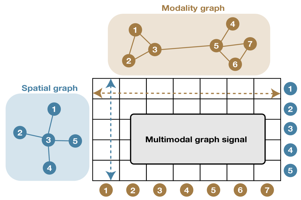
Figure 1: A multimodal graph signal on a twofold graph.

Notation: The notation of this paper is summarized in Table. I. We consider a weighted undirected graph $\mathcal{G}=(\mathcal{V},\mathcal{E})$, where $\mathcal{V}=\{v_{0},\ldots,v_{N-1}\}$ and $\mathcal{E}\subseteq\mathcal{V}\times\mathcal{V}$ represent sets of nodes and edges, respectively. Unless otherwise specified, $N=|\mathcal{V}|$ represents the number of nodes. The adjacency matrix of $\mathcal{G}$ is denoted by $\mathbf{W}$, where the $(i,j)$-element of $\mathbf{W}$, $w_{i,j}\geq 0$, is the edge weight between the $i$th and $j$th nodes; $w_{i,j}=0$ for unconnected nodes. The degree matrix $\mathbf{D}$ is defined as $\mathbf{D}=\textrm{diag}(d_{0},\ldots,d_{N-1})$, where $d_{i}=\sum_{j}w_{i,j}$ is the $i$th diagonal element. We use graph Laplacian $\mathbf{L}:=\mathbf{D}-\mathbf{W}$ as a graph operator. We can arbitrarily assign indices of edges as $\mathcal{E}=\{e_{q}\}_{q=0}^{|\mathcal{E}|-1}$. The weighted graph incidence matrix of $\mathcal{G}$ is defined as $\mathbf{M}\in\mathbb{R}^{|\mathcal{E}|\times N}$, where the $(p,q)$-element of $\mathbf{M}$ is defined as follows:

$$[\mathbf{M}]_{p,q}=\begin{dcases}\sqrt{w_{i,j}}&\textrm{if $p=i$ and $e_{q}=(v_{i},v_{j})$}\\ -\sqrt{w_{i,j}}&\textrm{if $p=j$ and $e_{q}=(v_{i},v_{j})$}\\ 0&\textrm{otherwise}.\end{dcases}$$

A graph signal $\mathbf{x}\in\mathbb{R}^{N}$ is defined as a mapping from the node set to the set of real numbers, i.e., $x_{i}:\mathcal{V}\rightarrow\mathbb{R}$. We assume that $\mathbf{x}$ is smooth on $\mathcal{G}$. The smoothness of $\mathbf{x}$ is measured using the Laplacian quadratic form $\mathbf{x}^{\top}\mathbf{L}\mathbf{x}$. If it is small, $\mathbf{x}$ is considered to be smooth on $\mathcal{G}$. The graph Fourier transform (GFT) of $\mathbf{x}$ is defined as $\hat{\mathbf{x}}=\mathbf{U}^{\top}\mathbf{x}$ where the GFT matrix $\mathbf{U}$ is obtained by the eigendecomposition of the graph Laplacian $\mathbf{L}=\mathbf{U\Lambda}\mathbf{U}^{\top}$ with the eigenvalue matrix $\mathbf{\Lambda}=\textrm{diag}(\lambda_{0},\ldots,\lambda_{N-1})$. We refer to $\lambda_{i}$ as a graph frequency.

The domain index is denoted by $e=\{s,m\}$, where $s$ and $m$ correspond to the spatial and modality domains, respectively. In this manner, spatial and modality graphs are denoted by $\mathcal{G}_{s}=(\mathcal{V}_{s},\mathcal{E}_{s},\mathbf{W}_{s})$ and $\mathcal{G}_{m}=(\mathcal{V}_{m},\mathcal{E}_{m},\mathbf{W}_{m})$, respectively. $N_{s}=|\mathcal{V}_{s}|$ and $N_{m}=|\mathcal{V}_{m}|$ represents the number of nodes of each graph. A multimodal graph signal is defined as $\mathbf{X}\in\mathbb{R}^{N_{s}\times N_{m}}$ (see Fig. 1).

TABLE I: Symbols used in this paper.

Symbols	Definitions
$x,\mathbf{x},\mathbf{X}$	scalar, vector, and matrix
$x_{i},[\mathbf{x}]_{i}$	$i$-th element of $\mathbf{x}$
$[\mathbf{X}]_{i,j}$	$(i,j)$-th element of $\mathbf{X}$
$[\mathbf{X}]_{i,:}$	$i$-th row vector of $\mathbf{X}$
$[\mathbf{X}]_{:,j}$	$j$-th column vector of $\mathbf{X}$
$\mathbf{1}_{N}$	all-ones vector with the length $N$
$\mathbf{I}_{N}$	identity matrix with the size $N\times N$
$\textrm{log}(\mathbf{x})$	vector with the logarithm of each element of $\mathbf{x}$
$\textrm{diag}(x_{0},\ldots,x_{N-1})$	diagonal matrix whose $(i,i)$-elements are $x_{i}$
$\textrm{Diag}(\mathbf{X})$	vector whose $i$-th elements are $[\mathbf{X}]_{i,i}$
$\textrm{tr}(\mathbf{X})$	trace of $\mathbf{X}$
$\|\mathbf{x}\|_{p}$	$\ell_{p}$ norm of $\mathbf{x}$
$\|\mathbf{X}\|_{F}$	Frobenius norm of $\mathbf{X}$
$\mathbf{X}^{\dagger}$	Moore-Penrose pseudoinverse of $\mathbf{X}$
$\mathbf{X}\circ\mathbf{Y}$	Hadamard product of $\mathbf{X}$ and $\mathbf{Y}$

II RELATED WORK

In this section, we review graph signal denoising and graph learning relevant to the formulation of the proposed method which is discussed below in Section III. First, We introduce existing model-based graph signal denoising methods [16, 12]. Then, representative graph learning approaches are shown [29, 27].

II-A GRAPH SIGNAL DENOISING

In a typical denoising setting, the following observation model is assumed:

$$\mathbf{y}=\mathbf{x}+\mathbf{n},$$ (1)

where $\mathbf{y}\in\mathbb{R}^{N}$ is the noisy observation, $\mathbf{x}\in\mathbb{R}^{N}$ is the unknown ground-truth signal, and $\mathbf{n}\in\mathbb{R}^{N}$ is additive white Gaussian noise (AWGN).

Signal denoising aims to recover $\mathbf{x}$ from $\mathbf{y}$ based on the assumption(s) on signal priors. Similar to time- and spatial-domain signal processing, we assume smoothness of the signal on the graph $\mathcal{G}$, where the smoothness is measured by the Laplacian quadratic form $\mathbf{x}^{\top}\mathbf{L}\mathbf{x}=\|\mathbf{L}^{1/2}\mathbf{x}\|_{2}^{2}$. Therefore, the well-known denoising with a Tikhonov regularization term is given as follows:

$$\min_{\mathbf{x}}\|\mathbf{y}-\mathbf{x}\|_{2}^{2}+\alpha\mathbf{x}^{\top}\mathbf{L}\mathbf{x},$$ (2)

where $\alpha>0$ is the regularization parameter. Note that, the regularization term acts as a graph high-pass filter since $\mathbf{L}^{1/2}\mathbf{x}=\mathbf{U}\hat{g}(\bm{\Lambda})\mathbf{U}^{\top}\mathbf{x}$ where the graph filter $\hat{g}(\lambda)=\lambda^{1/2}$. As a result, minimizing (2) promotes smoothness of graph signals.

We can easily obtain the solution of (2) in a closed form:

$$\widetilde{\mathbf{x}}=(\mathbf{I}_{N}+\alpha\mathbf{L})^{-1}\mathbf{y}=\mathbf{U}(\mathbf{I}_{N}+\alpha\mathbf{\Lambda})^{-1}\mathbf{U}^{\top}\mathbf{y}.$$ (3)

Denoting by $\hat{h}(\mathbf{\Lambda})=(\mathbf{I}+\alpha\mathbf{\Lambda})^{-1}$, (3) can be interpreted as a low-pass filter with the graph spectral kernel $\hat{g}(\lambda)=1/(1+\alpha\lambda)$.

Beyond the Tikhonov regularization, a variety of filter kernels has been considered [16, 30, 17, 31, 18]. Note that any smoothing filter can be applied to our framework as long as it fits our formulation.

The above-mentioned observation model in (1) is the single modal case where each node is associated with a scalar. In the multimodal setting, we easily extend the signal observation model as follows:

$$\mathbf{Y}=\mathbf{X}+\mathbf{N},$$ (4)

where $\mathbf{X}$, $\mathbf{Y}$, $\mathbf{N}\in\mathbb{R}^{N_{s}\times N_{m}}$ are the unknown ground-truth signal, noisy measurement, and AWGN, respectively. In this case, the $(i,k)$ element of a matrix corresponds to the signal value at node $i$ and modal $k$.

Similar to the single-modal case, multimodal signal denoising aims to recover $\mathbf{X}$ from $\mathbf{Y}$ by utilizing signal priors. In [12], multimodal graph signal denoising is introduced similar to the single modal case under the given twofold graph. However, in a practical case, the twofold graph is not given, both for the spatial and modality graphs.

II-B GRAPH LEARNING

Many GSP techniques assume graph Laplacian is given a priori. However, this is not often the case: We need to estimate/learn graphs from prior knowledge or given data. The classical method is $k$-nearest neighbor which has still been widely used [32]. However, the obtained graph does not always reflect the statistics of observed signals.

As a more data-driven graph estimation approach, graph learning has been widely studied in GSP[28, 27, 33, 34]. Let $\mathbf{X}_{\textrm{single}}=\begin{bmatrix}\mathbf{x}_{0},\dots,\mathbf{x}_{K-1}\end{bmatrix}\in\mathbb{R}^{N\times K}$ be a collection of $K$ single modal graph signals on a spatial graph. Note that the column does not refer to modality in contrast to (4).

A typical goal of graph learning is to estimate a graph Laplacian $\mathbf{L}$ from $\mathbf{X}_{\textrm{single}}$. Assuming the signal smoothness, a graph learning problem is often given as follows:

$$\min_{\mathbf{L}\in\mathcal{L}}\textrm{tr}(\mathbf{X}_{\textrm{single}}^{\top}\mathbf{L}\mathbf{X}_{\textrm{single}})+f_{L}(\mathbf{L}),$$ (5)

where $\mathcal{L}=\{\mathbf{L}\in\mathbb{R}^{N\times N}~|~\mathbf{L}\mathbf{1}_{N}=\mathbf{0},~[\mathbf{L}]_{i,j}=[\mathbf{L}]_{j,i}\leq 0~(i\neq j)\}$ is the feasible set of graph Laplacians and $f_{L}(\mathbf{L})$ is a regularization function with respect to $\mathbf{L}$. Since the first term in (5) is nothing but the Laplacian quadratic form, it promotes the smoothness of signals on the graph. Many regularization functions $f_{L}(\mathbf{L})$ have been proposed in literature: For example, $f_{L}(\mathbf{L})=\gamma\|\mathbf{L}\|_{F}^{2}$ where $\gamma>0$ is the regularization parameter in [28]. Constraints on time-varying graph learning has also been proposed in [34].

A similar expression of graph learning to (5) based on adjacency matrix has been proposed in [27]. It utilizes a distance matrix $\mathbf{Z}\in\mathbb{R}^{N\times N}$ whose element is given by

$$[\mathbf{Z}]_{i,j}=\|[\mathbf{X}_{\textrm{single}}]_{i,:}-[\mathbf{X}_{\textrm{single}}]_{j,:}\|_{2}^{2}.$$ (6)

We can then rewrite (5) with $\mathbf{Z}$ as follows:

$$\min_{\mathbf{W}\in\mathcal{W}}\|\mathbf{W}\circ\mathbf{Z}\|_{1}+f_{W}(\mathbf{W}),$$ (7)

where $\mathcal{W}=\{\mathbf{W}\in\mathbb{R}^{N\times N}_{\geq 0}~|~\mathbf{W}=\mathbf{W}^{\top},[\mathbf{W}]_{i,i}=0\}$ is the feasible set of adjacency matrices and $f_{W}(\mathbf{W})$ is an arbitrary regularization function with respect to $\mathbf{W}$.

The first term in (7) is equivalent to $2\textrm{tr}(\mathbf{X}_{\textrm{single}}^{\top}\mathbf{L}\mathbf{X}_{\textrm{single}})$ and it corresponds to the signal smoothness term in (5). Also, many versions of $f_{W}(\mathbf{W})$ have been presented (see [29] and references therein): For example, $f_{W}(\mathbf{W})$ is defined as follows in [27]:

$$f_{W}(\mathbf{W})=-\beta\mathbf{1}_{N}^{\top}\log(\mathbf{W}\mathbf{1}_{N})+\frac{\gamma}{2}\|\mathbf{W}\|_{F}^{2},$$ (8)

where $\beta>0$ and $\gamma>0$ are parameters. The first term controls the connectivity of the graph, where a larger $\beta$ promotes dense connections. The second term regularizes the edge weights, where a larger $\gamma$ results in smaller edge weights.

Note that, while [28] considers a joint problem of graph learning and smoothing signals, multimodal versions with twofold graphs have not been presented so far. In the following section, we introduce our proposed method by simultaneously considering signal smoothing and twofold graph learning.

III MULTIMODAL GRAPH SIGNAL DENOISING WITH SIMULTANEOUS GRAPH LEARNING

As mentioned above, existing graph signal denoising methods assume the underlying graph is given prior to denoising. They also assume signals are single-modal. However, they are not often the case. In this section, we propose a denoising method for multimodal graph signals by learning twofold graphs simultaneously. The overview of our method is illustrated in Fig. 2.

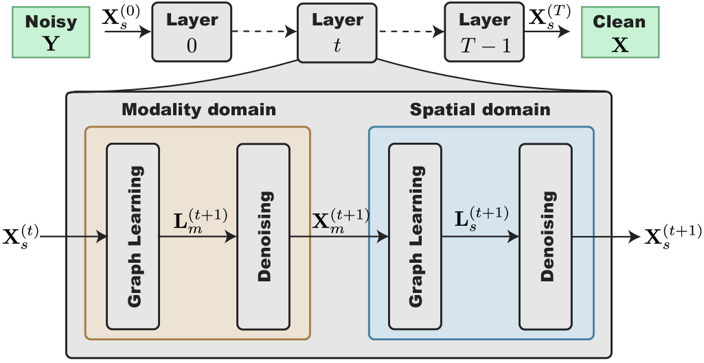
Figure 2: Overview of the proposed architecture.

III-A PROBLEM FORMULATION

We consider the measurement model $\mathbf{Y}=\mathbf{X}+\mathbf{N}$ in (4). We aim to restore $\mathbf{X}$ from $\mathbf{Y}$ by simultaneously learning a spatial graph $\mathcal{G}_{s}$ and a modality graph $\mathcal{G}_{m}$.

Here, we assume the joint smoothness on the twofold graph: Each column of $\mathbf{X}$ is smooth on $\mathcal{G}_{s}$ and each row of $\mathbf{X}$ is smooth on $\mathcal{G}_{m}$. Based on the smoothness assumption, we naturally extend the denoising for the single modal case in (2) to the multimodal case as follows:

$$\min_{\mathbf{X},\mathbf{L}_{s}\in\mathcal{L}_{s},\mathbf{L}_{m}\in\mathcal{L}_{m}}~\|\mathbf{Y}-\mathbf{X}\|_{F}^{2}+f_{s}(\mathbf{X},\mathbf{L}_{s})+f_{m}(\mathbf{X}^{\top},\mathbf{L}_{m}),$$ (9)

where $\mathcal{L}_{e}=\{\mathbf{L}_{e}\in\mathbb{R}^{N_{e}\times N_{e}}~|~\mathbf{L}_{e}\mathbf{1}_{N_{e}}=\mathbf{0},~[\mathbf{L}_{e}]_{i,j}=[\mathbf{L}_{e}]_{j,i}\leq 0~(i\neq j)\}$ is the set of valid graph Laplacians for $e\in\{s,m\}$ and $f_{e}(\cdot)$ is a function with respect to multimodal graph signals $\mathbf{X}$ and graph Laplacian $\mathbf{L}_{e}$.

Since we consider a joint problem of signal smoothing and graph learning, the regularization term $f_{e}(\cdot)$ should reflect the both constraints. In this paper, we consider the following $f_{e}(\cdot)$ as an extension of that used in [28, 27]:

$${f}_{e}(\mathbf{X}_{e},\mathbf{L}_{e})= \alpha_{e}\textrm{tr}(\mathbf{X}_{e}^{\top}\mathbf{L}_{e}\mathbf{X}_{e})-\beta_{e}\mathbf{1}_{N_{e}}^{\top}\log(\textrm{diag}(\mathbf{L}_{e}))$$ (10)

$$+\frac{\gamma_{e}}{2}\|\bm{\Omega}_{e}\circ\mathbf{L}_{e}\|_{F}^{2},$$

where $\alpha_{e}$, $\beta_{e}$, and $\gamma_{e}$ are positive parameters, and $\bm{\Omega}_{e}\in\{0,1\}^{N_{e}\times N_{e}}$ is a matrix which extracts off-diagonal elements of $\mathbf{L}_{e}$. The first, second, and third terms in (10) promote signal smoothness on the graph, node connectivity, and sparseness of edge weights.

Note that (9) with (10) is jointly nonconvex. In this paper, we split it into the following convex optimization problems for graph signals ($\mathbf{X}_{e}$) and graph Laplacians ($\mathbf{L}_{e}$) as follows:

$$\min_{\mathbf{X}_{m}}\|\mathbf{Y}^{\top}-\mathbf{X}_{m}\|_{F}^{2}+\alpha_{m}\textrm{tr}(\mathbf{X}_{m}^{\top}\mathbf{L}_{m}\mathbf{X}_{m}),$$ (11a)

$$\min_{\mathbf{X}_{s}}\|\mathbf{X}_{m}^{\top}-\mathbf{X}_{s}\|_{F}^{2}+\alpha_{s}\textrm{tr}(\mathbf{X}_{s}^{\top}\mathbf{L}_{s}\mathbf{X}_{s}),$$ (11b)

$$\min_{\mathbf{L}_{m}\in\mathcal{L}_{m}}f_{m}(\mathbf{X}_{m},\mathbf{L}_{m}),$$ (11c)

$$\min_{\mathbf{L}_{s}\in\mathcal{L}_{s}}f_{s}(\mathbf{X}_{s},\mathbf{L}_{s}).$$ (11d)

As mentioned in Section III, (11a) and (11b) have the closed form solutions. Later, we also introduce that (11c) and (11d) can be solved by an iterative algorithm using primal-dual splitting (PDS) [35] after appropriate transformations. Therefore, if the parameters $\{\alpha_{e},\beta_{e},\gamma_{e}\}$ for $e\in\{s,m\}$ are fixed, each of the subproblems is convex. Note that we train the parameters via DAU from the training data (Section III-III-C) to promote fewer iterations.

III-B Internal Iterative Algorithm

Here, we provide the solutions to (11c) and (11d) using PDS algorithm. In this paper, we consider undirected graphs without self-loops. This means we can distinguish the graph Laplacian with its (lower or upper) triangular components $\bm{\ell}_{e}\in\mathbb{R}^{N_{e}(N_{e}-1)/2}$. Let us define $\textrm{vec}(\mathbf{L}_{e})\in\mathbb{R}^{N_{e}^{2}}$ as the vectorized version of $\mathbf{L}_{e}$. By using $\bm{\ell}_{e}$, $\mathbf{L}_{e}$ can be represented as follows:

$$\textrm{vec}(\mathbf{L}_{e})=\bm{\Phi}_{e}\bm{\ell}_{e},$$ (12)

where $\bm{\Phi}_{e}\in\{-1,0,1\}^{N_{e}^{2}\times\frac{N_{e}(N_{e}-1)}{2}}$ is the duplication matrix [36]. By using the relationship in (12), each term in (11c) and (11c) can be rewritten as follows:

$$\textrm{tr}(\mathbf{X}_{e}^{\top}\mathbf{L}_{e}\mathbf{X}_{e}) =\textrm{vec}(\mathbf{X}_{e}\mathbf{X}_{e}^{\top})^{\top}\bm{\Phi}_{e}\bm{\ell}_{e},$$ (13)

$$\mathbf{1}_{N_{e}}^{\top}\textrm{log}(\textrm{diag}(\textbf{L}_{e})) =\mathbf{1}_{N_{e}}^{\top}\textrm{log}(\bm{\Psi}_{e}\bm{\ell}_{e}),$$

$$\|\bm{\Omega}_{e}\circ\mathbf{L}_{e}\|_{F}^{2} =2\|\bm{\ell}_{e}\|_{2}^{2},$$

where $\bm{\Psi}_{e}\in\{-1,0\}^{N_{e}\times\frac{N_{e}(N_{e}-1)}{2}}$ is the matrix of a linear operator that satisfies $\textrm{diag}(\mathbf{L}_{e})=\bm{\Psi}_{e}\bm{\ell}_{e}$. As a result, we can rewrite (10) as follows:

$$\min_{\bm{\ell}_{e}} \alpha_{e}\textrm{vec}(\mathbf{X}_{e}\mathbf{X}_{e}^{\top})^{\top}\bm{\Phi}_{e}\bm{\ell}_{e}-\beta_{e}\mathbf{1}_{N_{e}}^{\top}\textrm{log}(\bm{\Psi}_{e}\bm{\ell}_{e})$$ (14)

$$+\gamma_{e}\|\bm{\ell}_{e}\|_{2}^{2}+\iota_{\cdot\leq\mathbf{0}}(\bm{\ell}_{e}),$$

where the last term expresses the constraint of the graph Laplacian using the indicator function $\iota_{\cdot\leq\mathbf{0}}$, which is defined by

$$\iota_{\cdot\leq\mathbf{0}}(\bm{\ell}_{e})=\begin{dcases}0&\textrm{if }\ell_{i}\leq 0\\ \infty&\textrm{otherwise}.\\ \end{dcases}$$ (15)

In fact, (14) can be solved iteratively with the PDS algorithm (detailed derivations are shown in Appendix). Its algorithm is shown in Algorithm 1 where we omit the index $e$ for simplicity.

III-C Deep Algorithm Unrolling

We utilize DAU for determine hyperparameters in Algorithm 1 to make the number of iterations smaller. We replace six hyperparameters $\{\alpha_{e},\beta_{e},\gamma_{e}\}$ for $e\in\{s,m\}$ in (10) with trainable ones as $\bm{\Theta}\coloneqq\{\alpha_{e}^{(t)}$, $\beta_{e}^{(t)}$, $\gamma_{e}^{(t)}\}_{t=0}^{T-1}$, where $T$ is the number of iterations (layers). We summarize the proposed denoising algorithm in Algorithm 2.

Our unrolled algorithm is trained to minimize the mean squared error (MSE) of multimodal signals as follows:

$$E(\bm{\Theta})=\frac{1}{N_{s}N_{m}}\|\mathbf{X}-\mathbf{X}^{\ast}\|_{F}^{2}$$ (16)

where $\mathbf{X}^{\ast}$ is the ground-truth multimodal graph signal. Note that all components are easily (sub-)differentiable and bounded-input-bounded-output. Therefore, all the parameters can be trained by back propagation.

Algorithm 1 PDS algorithm for solving (14)

Input: $\mathbf{X},\bm{\Phi},\bm{\Psi},\alpha=\alpha^{(t)},\beta=\beta^{(t)},\gamma=\gamma^{(t)},\theta,\textrm{tolerance }\epsilon$

1:Initialization: $\bm{\ell}^{(0)}=-\mathbf{1}/10,\mathbf{b}_{0}^{(0)}=\bm{\Psi}\bm{\ell}^{(0)}$ $i=0,\ldots,i_{\textrm{max}}-1$

2:$\mathbf{z}^{(i)}\leftarrow\bm{\ell}^{(i)}-\theta(\alpha\bm{\Phi}^{\top}\textrm{vec}(\mathbf{XX}^{\top})+2\gamma\bm{\ell}^{(i)}+\bm{\Psi}^{\top}\mathbf{b}_{0}^{(i)})$

3:$\mathbf{z}_{0}^{(i)}\leftarrow\mathbf{b}_{0}^{(i)}+\theta\bm{\Psi}\bm{\ell}^{(i)}$

4:$\mathbf{p}^{(i)}\leftarrow\textrm{prox}_{\theta\iota_{\cdot\leq\mathbf{0}}}(\mathbf{z}^{(i)})$

5:$\mathbf{p}_{0}^{(i)}\leftarrow\mathbf{z}_{0}^{(i)}-\theta\textrm{prox}_{\frac{1}{\theta}(-\beta\mathbf{1}_{\mathcal{V}}^{\top}\log(\cdot))}\left(\frac{\mathbf{z}_{0}^{(i)}}{\theta}\right)$

6:$\mathbf{q}^{(i)}\leftarrow\mathbf{p}^{(i)}-\theta(\alpha\bm{\Phi}^{\top}\textrm{vec}(\mathbf{XX}^{\top})+2\gamma\mathbf{p}^{(i)}+\bm{\Psi}^{\top}\mathbf{p}_{0}^{(i)})$

7:$\mathbf{q}_{0}^{(i)}\leftarrow\mathbf{p}_{0}^{(i)}+\theta\bm{\Psi}\mathbf{p}^{(i)}$

8:$\bm{\ell}^{(i+1)}\leftarrow\bm{\ell}^{(i)}-\mathbf{z}^{(i)}+\mathbf{q}^{(i)}$

9:$\mathbf{b}_{0}^{(i+1)}\leftarrow\mathbf{b}_{0}^{(i)}-\mathbf{z}_{0}^{(i)}+\mathbf{q}_{0}^{(i)}$ $\|\bm{\ell}^{(i+1)}-\bm{\ell}^{(i)}\|/\|\bm{\ell}^{(i)}\|<\epsilon$

10:break

Output: $\bm{\ell}^{(i+1)}$

Algorithm 2 MGSD-LLap-DAU: Multimodal graph signal denoising with simultaneously learning Laplacian matrix using deep algorithm unrolling

Input: $\mathbf{X}_{s}^{(0)}=\mathbf{Y},T,\{\alpha_{e}^{(t)},\beta_{e}^{(t)},\gamma_{e}^{(t)}\}_{t=0}^{T-1}~(e\in\{m,s\})$

$t=0,\ldots,T-1$

1:$\mathbf{L}_{m}^{(t+1)}\leftarrow\mathop{\rm arg~min}\limits_{L_{m}}f_{m}((\mathbf{X}_{s}^{(t)})^{\top},\mathbf{L}_{m})$

2:$\mathbf{X}_{m}^{(t+1)}\leftarrow(\mathbf{I}_{N_{m}}+\alpha_{m}^{(t)}\mathbf{L}_{m}^{(t+1)})^{-1}\mathbf{Y}^{\top}$

3:$\mathbf{L}_{s}^{(t+1)}\leftarrow\mathop{\rm arg~min}\limits_{L_{s}}f_{s}((\mathbf{X}_{m}^{(t+1)})^{\top},\mathbf{L}_{s})$

4:$\mathbf{X}_{s}^{(t+1)}\leftarrow(\mathbf{I}_{N_{s}}+\alpha_{s}^{(t)}\mathbf{L}_{s}^{(t+1)})^{-1}(\mathbf{X}_{m}^{(t+1)})^{\top}$

Output: $\mathbf{X}=\mathbf{X}_{s}^{(T)},\mathbf{L}_{m}^{(T)},\mathbf{L}_{s}^{(T)}$

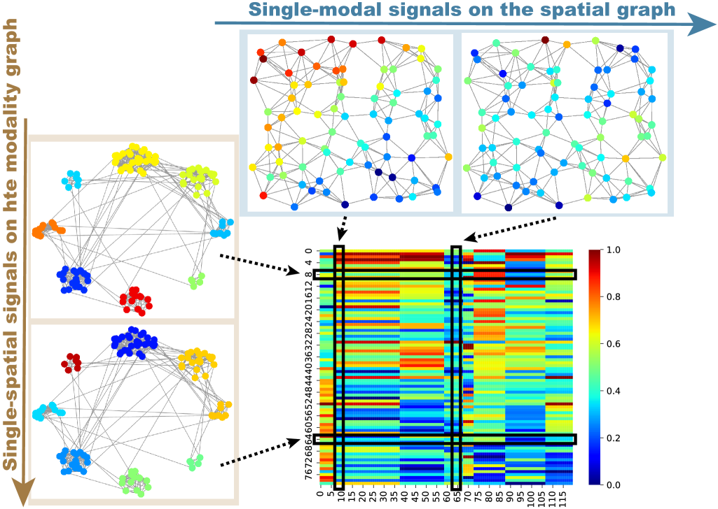
Figure 3: Visualization of synthetic multimodal graph signals.

TABLE II: RMSE of denoised signals for synthetic dataset.

	RMSE
Methods \$\sigma$	0.10	0.15	0.20	0.25	0.30
GLPF	0.084	0.122	0.171	0.224	0.283
HD	0.203	0.198	0.188	0.183	0.194
SVDS	0.100	0.149	0.199	0.249	0.299
AE	0.261	0.261	0.261	0.261	0.261
GCN	0.209	0.205	0.204	0.200	0.195
TGSR-DAU	0.068	0.091	0.117	0.138	0.155
MGSD-LLAP-DAU	0.030	0.039	0.051	0.060	0.076

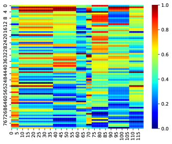
(a) Original

(b) Observed (0.30)

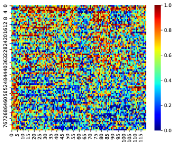
(c) GLPF (0.27)

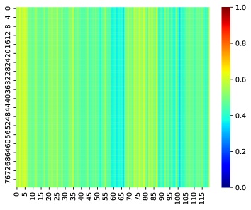
(d) HD (0.22)

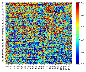
(e) SVDS (0.30)

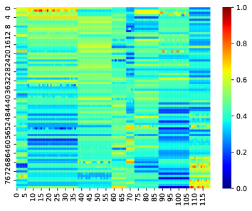
(f) AE (0.24)

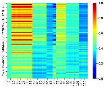
(g) GCN (0.19)

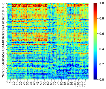
(h) TGSR-DAU (0.16)

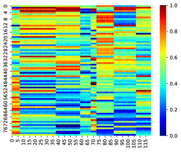
(i) MGSD-LLAP-DAU (0.07)

Figure 4: Denoising results for synthetic dataset ($\sigma=0.30$). The vertical indices correspond to the spatial graph numbers and the horizontal ones are the modality. Parenthesized values in subcaptions are RMSE.

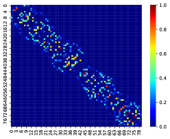
(a) Groundtruth

(b) Layer 1

(c) Layer 2

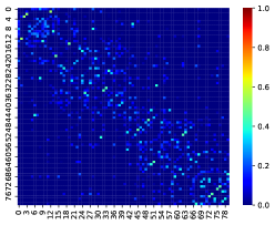
(d) Layer 3

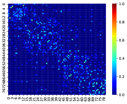
(e) Layer 4

(f) Layer 5

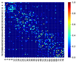
(g) Layer 6

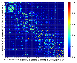
(h) Layer 7

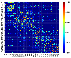
(i) Layer 8

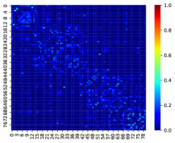
(j) Layer 9

Figure 5: Visualization of learned spatial graph $\mathbf{W}_{s}$ for synthetic dataset.

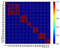
(a) Groundtruth

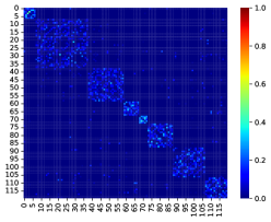
(b) Layer 1

(c) Layer 2

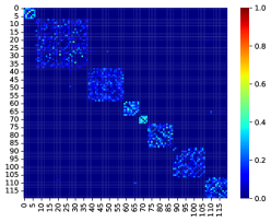
(d) Layer 3

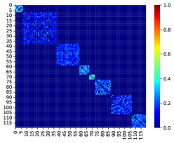
(e) Layer 4

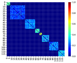
(f) Layer 5

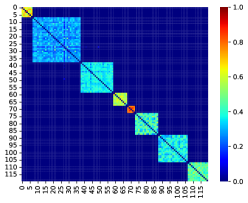
(g) Layer 6

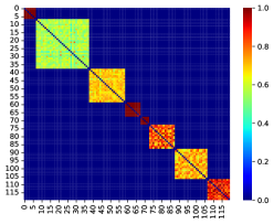
(h) Layer 7

(i) Layer 8

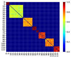
(j) Layer 9

Figure 6: Visualization of learned modality graph $\mathbf{W}_{m}$ for synthetic dataset.

IV DENOISING EXPERIMENTS

In this section, we perform denoising experiments of multimodal signals with synthetic and real-world datasets.

IV-A SETUP

IV-A1 DATASETS

We use the following two datasets.

Synthetic Dataset: As a ground-truth twofold graph, we use a random sensor graph as a spatial graph $\mathcal{G}_{s}$ and a community graph [37]. This setup reflects a typical measurement condition of wireless sensor networks or IoT with environmental sensors.

The spatial graph $\mathcal{G}_{s}$ is constructed as a $k$-nearest neighbor (kNN) graph with $k=6$, based on the coordinates of the nodes. The edge weights of $\mathcal{G}_{s}$ are determined based on their Euclidean distances in space and are rescaled to $[0,1]$.

We generated a modality graph $\mathcal{G}_{m}$ with eight clusters ($P=8$). First, all nodes within the same cluster are connected. Then, all pairs of inter-cluster nodes are connected with a probability of $1/N_{m}$. Edge weights for the modality graph are unweighted, i.e., $w_{i,j}=1$. We set $N_{s}=80$ and $N_{m}=120$.

The edge weights of $\mathcal{G}_{m}$ are set to be unweighted ($\{0,1\}$) based on the cluster.

Synthetic multimodal graph signals are obtained through two steps:

1. A spatial graph signal $\tilde{\mathbf{x}}_{p}\in\mathbb{R}^{N}$ is designed such that it varies smoothly on $\mathcal{G}_{s}$. It has been made to conform to a Gaussian Markov Random Field (GMRF) process [38], i.e., $\tilde{\mathbf{x}}_{p}\sim\mathcal{N}(\mathbf{0},\mathbf{L}_{s}^{\dagger})$, where $\mathbf{L}_{s}^{\dagger}$ is the Moore-Penrose pseudoinverse of $\mathbf{L}_{s}$.

2. Based on $\tilde{\mathbf{x}}_{p}$, we then modify the signal values to be correlated along the modality direction. We assume that multimodal signals are piecewise constant [39] on the modality graph. Therefore, the measurement matrix $\mathbf{X}$ is given by $\mathbf{X}=\begin{bmatrix}\tilde{\mathbf{x}}_{0}\mathbf{1}_{\mathcal{C}_{0}}^{\top}\cdots\tilde{\mathbf{x}}_{P-1}\mathbf{1}_{\mathcal{C}_{P-1}}^{\top}\end{bmatrix}$ where $\mathcal{C}_{p}$ is the set of nodes in the $p$th cluster of $\mathcal{G}_{m}$.

We visualize synthetic multimodal graph signals in Fig. 3.

For the experiments, we generate ten multimodal graphs. For each graph, experiments with five noise levels, $\sigma\in\{0.10,0.15,0.20,0.25,0.30\}$, are performed. Parameters are determined with a $2\times 2$ cross-validation.

TABLE III: RMSE of denoised signals for real-world dataset.

	RMSE
Methods \$\sigma$	3	5	7	9
GLPF	1.937	3.154	5.346	7.925
HD	2.982	3.800	4.838	6.046
SVDS	2.988	4.990	6.952	9.006
AE	3.776	3.776	3.776	3.776
GCN	3.437	3.266	3.406	4.082
TGSR-DAU	2.394	2.834	3.386	4.072
MGSD-LLAP-DAU	1.446	1.520	1.693	2.114

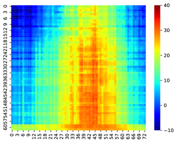
(a) Original

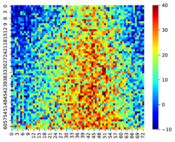
(b) Observed (9.00)

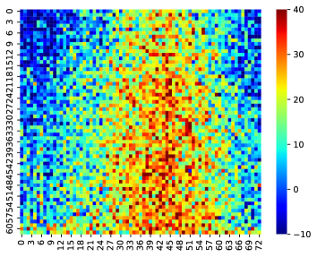
(c) GLPF (8.00)

(d) HD (8.53)

(e) SVDS (8.95)

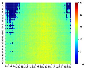
(f) AE (5.92)

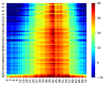
(g) GCN (5.19)

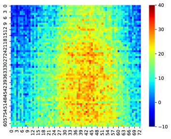
(h) TGSR-DAU (4.19)

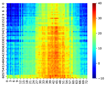
(i) MGSD-LLAP-DAU (2.31)

Figure 7: Denoising results for real-world dataset ($\sigma=9$). The vertical indices correspond to the spatial graph numbers and the horizontal ones are the modality. Parenthesized values in subcaptions are RMSE.

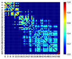
(a) Layer 1

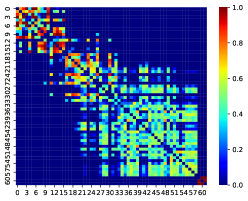
(b) Layer 2

(c) Layer 3

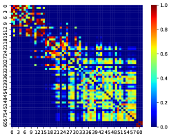
(d) Layer 4

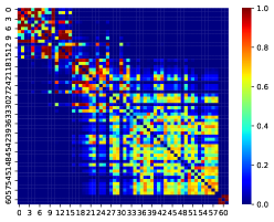
(e) Layer 5

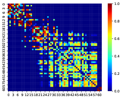
(f) Layer 6

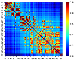
(g) Layer 7

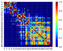
(h) Layer 8

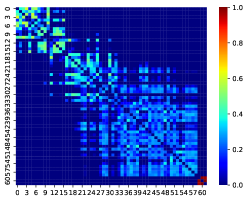
(i) Layer 9

Figure 8: Visualization of learned spatial graph $\mathbf{W}_{s}$ for real-world dataset.

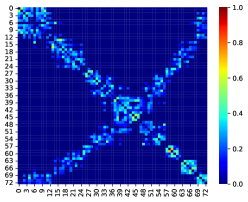
(a) Layer 1

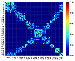
(b) Layer 2

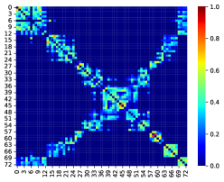
(c) Layer 3

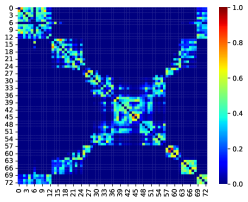
(d) Layer 4

(e) Layer 5

(f) Layer 6

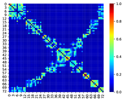
(g) Layer 7

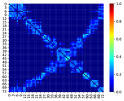
(h) Layer 8

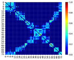
(i) Layer 9

Figure 9: Visualization of learned modality graph $\mathbf{W}_{m}$ for real-world dataset.

Real-world Dataset: We also perform denoising experiments using Japanese climate data publicly available from the Japan Meteorological Agency (JMA). In this experiment, we consider modality as seasons.

We utilize the temperature data consisting of daily average temperatures spanning ten years from 2013 to 2022, measured at 62 locations across Japan. To align the number of days in each year, data for February 29th in leap years have been excluded. The 62 locations were selected from observatories in Japan that had non-missing temperature data for the entire ten-year period.

The observed signals are made by the following two steps:

1. By performing five-day averaging, we have 73 sets of temperature data. This forms the original signals $\mathbf{X}\in\mathbb{R}^{62\times 73}$.

2. We then add AWGN ($\sigma\in\{3,5,7,9\}$) to the data to obtain the observed signal $\mathbf{Y}$.

Finally, we repeat the above two steps ten times to arrange $40$ pairs of $\{\mathbf{X},\mathbf{Y}\}$. We performed $2\times 2$ cross-validation for the dataset.

IV-A2 COMPARISON METHODS

We compare the denoising performance of the proposed method with the following existing methods:

• Graph low-pass filter (GLPF): $h(\lambda)=1/(1+\tau_{2}\lambda)$ [16],

• Diffusion with heat kernel (HD): $h(\lambda)=\exp(-\tau_{1}\lambda)$ [18],

• Singular value decomposition with hard shrinkage (SVDS) [31],

• Autoencoder (AE) [40],

• Graph convolutional network (GCN) [19],

• Graph signal denoising via twofold graph smoothness regularization with DAU (TGSR-DAU) [12].

The first three methods are model-based approaches, the fourth and fifth ones are deep learning-based ones, and the last is a DAU-based one.

In this paper, we assume that graphs are not given a priori. Therefore, we construct (spatial and modality) graphs using the Gaussian RBF kernel [41] for HD, GLPF, GCN, and TGSR-DAU. Note that HD, GLPF, and GCN can perform only on $\mathcal{G}_{s}$, i.e., they do not consider the modality direction. The parameters used in model-based methods (HD, GLPF, and SVDS) are fitted with Bayesian parameter estimation [42]. AE, GCN, TGSR-DAU, and the proposed method are trained the weights and the parameters from the training data, and the layers of the models are fitted $T=9$. Deep learning- and DAU-based methods are trained for 30 epochs using Adam optimizer [43] whose learning rate is set to 0.01. We use average of root mean square error (RMSE) as evaluation metrics.

IV-B Denoising Results of Synthetic Dataset

IV-B1 Quantitative and Qualitative Results

The denoising results are presented in Table II. As shown in the table, the proposed method maintains low RMSEs under all noise situations. This indicates that leveraging the inter-modality relationship through the simultaneous graph learning process is effective for denoising of multimodal graph signals.

The proposed method shows a robust performance with various noise strengths compared to GLPF and TGSR-DAU. This is because GLPF and TGSR-DAU directly use noisy signals for graph construction, making them noise-sensitive. In contrast, twofold graph learning phases in our method can handle noisy signals well. HD, AE, and GCN show similar reconstruction errors across different noise levels, suggesting over-smoothing along the spatial direction (as shown in Fig. 4).

The visualization results are shown in Fig. 4. Model-based methods such as GLPF, HD, and SVDS tend to have limited denoising performances or oversmoothing has occurred. AE and GCN, which are deep learning-based methods, extract clusters in the spatial domain, but the denoised signals have a low dynamic range. In contrast, the proposed method has high denoising performance due to the sequential learning of spatial and modality graphs.

IV-B2 Learned Graphs

The adjacency matrices of the graphs estimated by the proposed method are shown in Figs. 5 and 6. The figures show the obtained graphs in a layer-by-layer manner. Basically, trained spatial graphs in the early layers (shown in Fig. 5(b)–(f)) have small edge weights: This implies the proposed method performs global denoising in the early stage. The edge weights are getting larger when the layer goes deeper. This could result in local denoising close to the output. The spatial graph at the last layer, Fig. 5(j), is very sparse which suggests that eight layers for the spatial signal denoising could be enough.

IV-C Denoising Results of Real-world Dataset

IV-C1 Quantitative and Qualitative Results

Table III shows the denoising results for the real-world temperature dataset. Similar to the synthetic signals, the proposed method shows smaller RMSE than the alternative methods. Note that, for a graph signal denoising task, model-based methods often perform better than the deep learning-based ones, especially for small noise cases. For large noises, deep learning-based methods are better than the model-based methods. However, the predefined graphs limit the performance: It could be solved by our approach. Note that AE may overfit to the data and produce the same outputs regardless of the input.

The visualization results are shown in Fig. 7. As the results of the synthetic dataset, GLPF, HD, and SVDS are not well performed and the resulting signals are quite similar to the noisy signal. AE and GCN oversmoothed and overenhanced the multimodal signal, respectively. TGSR-DAU can denoise the signal partially but noises still remain. As observed, the proposed method is able to denoise the multimodal signal using both temporal and spatial information.

IV-C2 Learned Graphs

The adjacency matrices of the graphs estimated by the proposed method are shown in Figs. 8 and 9. Similar to the synthetic data, the graphs obtained in the first layer have low edge weights which results in global denoising. In the following layers, edge weights are almost consistent until the seventh or eighth layers: These layers could correspond to local denoising.

In the spatial graph shown in Fig. 8, nodes having close indices are likely to be connected that reflects geographic similarities: The station (i.e., node) indices are assigned from north to south. Several softly-separated clusters are also observed. This corresponds to similar climate regions in Japan: From top left to bottom right, clusters indicate the following regions: Hokkaido/Tohoku, Kanto, Chubu/Western Japan, and other isolated islands (very small cluster at the bottom right).

In the modality graph shown in Fig. 9, edges are drawn between nodes with similar indices, suggesting a positive correlation between signals from nearby dates. Furthermore, nodes (i.e., dates) having similar climates are also connected. For example, nodes 0 to 12 (early January to early March) are connected to nodes 66 to 72 (late November to late December), which reflects seasonal behavior of climates in Japan.

V CONCLUSION

This paper presents a simultaneous method of multimodal signal denoising on a twofold graph and graph learning using DAU. The proposed algorithm alternates graph learning and signal denoising both for the spatial and modality domains. We solve the iterative optimization by DAU where the parameters in the iterations are automatically tuned with training data. The numerical results demonstrate that the proposed method is effective for denoising multimodal signals compared to conventional methods.

[Derivation of Iterative Algorithm for (14)] PDS is an algorithm designed to solve a minimization problem written as follows:

$$\min_{\bm{\ell}}g_{0}(\bm{\ell})+g_{1}(\bm{\Psi}\bm{\ell})+g_{2}(\bm{\ell}),$$ (17)

where $g_{0}$ and $g_{1}$ are proximable proper lower semicontinuous convex functions, and $g_{2}$ is a differentiable convex function whose gradient $\nabla g_{3}$ has a Lipschitz constant. Applying (17) to our problem, each term in (14) can be assigned as follows:

$$g_{0}(\bm{\ell}_{e}) =\iota_{\cdot\leq\mathbf{0}}(\bm{\ell}_{e}),$$ (18)

$$g_{1}(\bm{\Psi}_{e}\bm{\ell}_{e}) =-\beta_{e}\mathbf{1}_{N_{e}}^{\top}\log(\bm{\Psi}_{e}\bm{\ell}_{e}),$$

$$g_{2}(\bm{\ell}_{e}) =\alpha_{e}\textrm{vec}(\mathbf{X}_{e}\mathbf{X}_{e}^{\top})^{\top}\bm{\Phi}_{e}\bm{\ell}_{e}+\gamma_{e}\|\bm{\ell}_{e}\|_{2}^{2}.$$

The proximal operator of $g_{0}$ and $g_{1}$, as well as $\nabla g_{2}$ are given by

$$\textrm{prox}_{\theta_{e}g_{0}}(\ell) =\min\{\ell,0\},$$ (19)

$$\textrm{prox}_{\theta_{e}g_{1}}(\ell) =\frac{\ell+\sqrt{\ell^{2}+4\beta_{e}\theta_{e}}}{2},$$

$$\nabla g_{2}(\bm{\ell}) =\alpha_{e}\bm{\Phi}_{e}^{\top}\textrm{vec}(\mathbf{X}_{e}\mathbf{X}_{e}^{\top})+2\gamma_{e}\bm{\ell},$$

where $\theta_{e}\in(0,+\infty)$ denotes the stepsize (refer to [35] for the conditions of algotrithm convergence).

References

- [1] K. Takanami, Y. Bandoh, S. Takamura, and Y. Tanaka, “Multimodadl Graph Signal Denoising With Simultaneous Graph Learning using Deep Algorithm Unrolling,” in 2023 IEEE Int Conf Image Process ICIP, Oct. 2023, pp. 1555–1559.
- [2] I. Akyildiz, W. Su, Y. Sankarasubramaniam, and E. Cayirci, “A survey on sensor networks,” IEEE Commun. Mag., vol. 40, no. 8, pp. 102–114, Aug. 2002.
- [3] I. F. Akyildiz, W. Su, Y. Sankarasubramaniam, and E. Cayirci, “Wireless sensor networks: A survey,” Comput. Netw., vol. 38, no. 4, pp. 393–422, Mar. 2002.
- [4] H. Alemdar and C. Ersoy, “Wireless sensor networks for healthcare: A survey,” Comput. Netw., vol. 54, no. 15, pp. 2688–2710, Oct. 2010.
- [5] “Wireless Sensor Networks - Smart Environments - Wiley Online Library.”
- [6] M. Tubaishat and S. Madria, “Sensor networks: An overview,” IEEE Potentials, vol. 22, no. 2, pp. 20–23, Apr. 2003.
- [7] R. Krishnamurthi, A. Kumar, D. Gopinathan, A. Nayyar, and B. Qureshi, “An Overview of IoT Sensor Data Processing, Fusion, and Analysis Techniques,” Sensors, vol. 20, no. 21, p. 6076, Jan. 2020.
- [8] D. B. Tay, “Sensor network data denoising via recursive graph median filters,” Signal Processing, vol. 189, p. 108302, Dec. 2021.
- [9] A. Ortega, P. Frossard, J. Kovacevic, J. M. F. Moura, and P. Vandergheynst, “Graph signal processing: Overview, challenges, and applications,” Proc. IEEE, vol. 106, no. 5, pp. 808–828, May 2018.
- [10] G. Leus, A. G. Marques, J. M. Moura, A. Ortega, and D. I. Shuman, “Graph Signal Processing: History, development, impact, and outlook,” IEEE Signal Process. Mag., vol. 40, no. 4, pp. 49–60, Jun. 2023.
- [11] Y. Tanaka, Y. C. Eldar, A. Ortega, and G. Cheung, “Sampling signals on graphs: From theory to applications,” IEEE Signal Process. Mag., vol. 37, no. 6, pp. 14–30, Jan. 2020.
- [12] M. Nagahama and Y. Tanaka, “Multimodal Graph Signal Denoising Via Twofold Graph Smoothness Regularization with Deep Algorithm Unrolling,” in ICASSP 2022 - 2022 IEEE Int. Conf. Acoust. Speech Signal Process. ICASSP, May 2022, pp. 5862–5866.
- [13] S. Chen, A. Sandryhaila, J. M. F. Moura, and J. Kovačević, “Signal Recovery on Graphs: Variation Minimization,” IEEE Trans. Signal Process., vol. 63, no. 17, pp. 4609–4624, Sep. 2015.
- [14] S. Ono, I. Yamada, and I. Kumazawa, “Total generalized variation for graph signals,” in 2015 IEEE Int. Conf. Acoust. Speech Signal Process. ICASSP, Apr. 2015, pp. 5456–5460.
- [15] Y. Yazaki, Y. Tanaka, and S. H. Chan, “Interpolation and denoising of graph signals using plug-and-play ADMM,” in Span Classnocaseieee-Icasspspan, 2019, pp. 5431–5435.
- [16] D. I. Shuman, S. K. Narang, P. Frossard, A. Ortega, and P. Vandergheynst, “The emerging field of signal processing on graphs: Extending high-dimensional data analysis to networks and other irregular domains,” IEEE Signal Process. Mag., vol. 30, no. 3, pp. 83–98, May 2013.
- [17] M. Onuki, S. Ono, M. Yamagishi, and Y. Tanaka, “Graph Signal Denoising via Trilateral Filter on Graph Spectral Domain,” IEEE Trans. Signal Inf. Process. Netw., vol. 2, no. 2, pp. 137–148, Jun. 2016.
- [18] F. Zhang and E. R. Hancock, “Graph spectral image smoothing using the heat kernel,” Pattern Recognit., vol. 41, no. 11, pp. 3328–3342, Nov. 2008.
- [19] T. N. Kipf and M. Welling, “Semi-supervised classification with graph convolutional networks,” in 2017 Int Conf Learn Represent ICLR. OpenReview.net, 2017.
- [20] X. Jian, W. P. Tay, and Y. C. Eldar, “Kernel Based Reconstruction for Generalized Graph Signal Processing,” IEEE Trans. Signal Process., vol. 72, pp. 2308–2322, 2024.
- [21] B. Khemani, S. Patil, K. Kotecha, and S. Tanwar, “A review of graph neural networks: Concepts, architectures, techniques, challenges, datasets, applications, and future directions,” Journal of Big Data, vol. 11, no. 1, p. 18, Jan. 2024.
- [22] S. Chen, Y. C. Eldar, and L. Zhao, “Graph Unrolling Networks: Interpretable Neural Networks for Graph Signal Denoising,” IEEE Trans. Signal Process., vol. 69, pp. 3699–3713, 2021.
- [23] K. Gregor and Y. LeCun, “Learning fast approximations of sparse coding,” Proc 27th Int Conf Mach. Learn., pp. 399–406, 2010.
- [24] V. Monga, Y. Li, and Y. C. Eldar, “Algorithm unrolling: Interpretable, efficient deep learning for signal and image processing,” IEEE Signal Process. Mag., vol. 38, no. 2, pp. 18–44, Mar. 2021.
- [25] M. Nagahama, K. Yamada, Y. Tanaka, S. H. Chan, and Y. C. Eldar, “Graph signal restoration using nested deep algorithm unrolling,” IEEE Trans. Signal Process., vol. 70, pp. 3296–3311, 2022.
- [26] C. Yang, M. Hu, G. Zhai, and X.-P. Zhang, “Graph-Based Denoising for Respiration and Heart Rate Estimation During Sleep in Thermal Video,” IEEE Internet Things J., vol. 9, no. 17, pp. 15 697–15 713, Sep. 2022.
- [27] V. Kalofolias, “How to learn a graph from smooth signals,” in Proc. 19th Int. Conf. Artif. Intell. Stat. PMLR, May 2016, pp. 920–929.
- [28] X. Dong, D. Thanou, P. Frossard, and P. Vandergheynst, “Learning laplacian matrix in smooth graph signal representations,” IEEE Trans. Signal Process., vol. 64, no. 23, pp. 6160–6173, Dec. 2016.
- [29] X. Dong, D. Thanou, M. Rabbat, and P. Frossard, “Learning graphs from data: A signal representation perspective,” IEEE Signal Process. Mag., vol. 36, no. 3, pp. 44–63, May 2019.
- [30] C. Tomasi and R. Manduchi, “Bilateral filtering for gray and color images,” in Sixth Int Conf Comp Vis. ICCV, Jan. 1998, pp. 839–846.
- [31] M. Gavish and D. L. Donoho, “The optimal hard threshold for singular values is $4/\sqrt 3$,” IEEE Trans. Inf. Theory, vol. 60, no. 8, pp. 5040–5053, Aug. 2014.
- [32] G. Mateos, S. Segarra, A. G. Marques, and A. Ribeiro, “Connecting the Dots: Identifying Network Structure via Graph Signal Processing,” IEEE Signal Process. Mag., vol. 36, no. 3, pp. 16–43, May 2019.
- [33] V. Kalofolias and N. Perraudin, “Large scale graph learning from smooth signals,” in 2019 Int Conf Learn Represent ICLR, 2019.
- [34] K. Yamada, Y. Tanaka, and A. Ortega, “Time-varying graph learning based on sparseness of temporal variation,” in 2019 IEEE Int Conf Acoust Speech Signal Process ICASSP. IEEE, May 2019, pp. 5411–5415.
- [35] N. Komodakis and J.-C. Pesquet, “Playing with duality: An overview of recent primal-dual approaches for solving large-scale optimization problems,” IEEE Signal Process. Mag., vol. 32, no. 6, pp. 31–54, Jan. 2015.
- [36] K. M. Abadir and J. R. Magnus, Matrix Algebra. Cambridge University Press, Aug. 2005.
- [37] N. Perraudin, J. Paratte, D. Shuman, L. Martin, V. Kalofolias, P. Vandergheynst, and D. K. Hammond, “GSPBOX: A toolbox for signal processing on graphs,” Mar. 2016.
- [38] H. Rue and L. Held, Gaussian Markov Random Fields: Theory and Applications. Chapman and Hall/CRC, Feb. 2005.
- [39] S. Chen, R. Varma, A. Singh, and J. Kovačević, “Representations of piecewise smooth signals on graphs,” in 2016 IEEE Int Conf Acoust Speech Signal Process ICASSP, Mar. 2016, pp. 6370–6374.
- [40] P. Vincent, H. Larochelle, I. Lajoie, Y. Bengio, and P.-A. Manzagol, “Stacked denoising autoencoders: Learning useful representations in a deep network with a local denoising criterion,” J Mach. Learn. Res., Dec. 2010.
- [41] S. S. Keerthi and C.-J. Lin, “Asymptotic behaviors of support vector machines with gaussian kernel,” Neural Comput., vol. 15, no. 7, pp. 1667–1689, Jul. 2003.
- [42] A. D. Bull, “Convergence rates of efficient global optimization algorithms,” J Mach. Learn. Res., vol. 12, no. 88, pp. 2879–2904, 2011.
- [43] D. P. Kingma and J. Ba, “Adam: A method for stochastic optimization,” in 3rd Int. Conf. Learn. Represent. ICLR 2015 San Diego CA USA May 7-9 2015 Conf. Track Proc., Y. Bengio and Y. LeCun, Eds., 2015.