Lifted Forward Planning in Relational Factored Markov Decision Processes with Concurrent Actions

Abstract

Decision making is a central problem in AI that can be formalized using a Markov Decision Process. A problem is that, with increasing numbers of (indistinguishable) objects, the state space grows exponentially. To compute policies, the state space has to be enumerated. Even more possibilities have to be enumerated if the size of the action space depends on the size of the state space, especially if we allow concurrent actions. To tackle the exponential blow-up in the action and state space, we present a first-order representation to store the spaces in polynomial instead of exponential size in the number of objects and introduce Foreplan, a relational forward planner, which uses this representation to efficiently compute policies for numerous indistinguishable objects and actions. Additionally, we introduce an even faster approximate version of Foreplan. Moreover, Foreplan identifies how many objects an agent should act on to achieve a certain task given restrictions. Further, we provide a theoretical analysis and an empirical evaluation of Foreplan, demonstrating a speedup of at least four orders of magnitude.

8114

1 Introduction

Decision making problems can be formalized using Markov Decision Processes (MDPs). To compute a policy for an MDP, the state and action spaces have to be enumerated to find the best possible action for each state. But, with increasing number of (indistinguishable) objects, the state space grows exponentially. In case the actions depend on the states or objects as well, even more possibilities have to be enumerated, let alone if further concurrent actions are allowed. For concurrent actions, all possible action combinations have to be enumerated, yielding an exponentially-sized action space, which is why concurrency is rarely modelled. However, consider the following example: A small town is haunted by an epidemic. To fight the epidemic, the town’s mayor can impose travel bans on the town’s citizens. Certainly, the mayor can confine all citizens to their homes, stopping the epidemic. However, the citizens’ overall welfare is important as well. Therefore, the mayor is interested in the best decision of imposing travel bans (concurrent actions) w.r.t. confining the epidemic, while keeping the citizens’ welfare above a certain threshold. In addition, there can be circumstances, where the policy has to be adapted, e.g., if a wave of infections is on the rise, threatening to infect the majority of the population. Computing this problem on a propositional level, with every citizen explicitly represented, like approaches such as MDPs do, blows up the state and action space, as it requires exponential enumeration of all subsets of the population. However, there are groups of citizens behaving identically w.r.t. getting sick (and well again) as well as regarding their welfare if a travel ban is imposed, i.e., these citizens are indistinguishable for the mayor. Within these groups, it does not matter on which exact citizen the mayor imposes a travel ban on, only on how many she imposes a travel ban on. Additionally, many computations over subsets of indistinguishable citizens are redundant. Thus, we propose to drastically reduce the search and action space by using a first-order representation, grouping indistinguishable citizens, and use this representation to plan group-wise by reasoning about a representative and then projecting the result to the whole group.

Contribution

First, to be able to represent numerous indistinguishable objects and actions, we use probabilistic relational models as a representation in (factored) MDPs (fMDPs), which yields relational factored MDPs (rfMDPs). Second, we propose Foreplan to carry out planning in rfMDPs. State of the art algorithms run in time exponential in the number of objects. To reduce the time taken to polynomial in the number of objects, we define the relational cost graph, which is used by Foreplan to encode the state and action space in an efficient way. Denoting the number of cliques by $c$ and the size of the largest clique by $w$ in the relational cost graph, Foreplan runs exponential in $c$ and $w$. Both parameters are structural ones, mostly small and fixed, and thus independent of the number of objects. Therefore, Foreplan is an efficient planner w.r.t the number of objects. Third, using approximation, we can reduce the runtime even further. We propose Approximate Foreplan, whose runtime is polynomial in $c$. For Approximate Foreplan, we show a speedup of at least four orders of magnitude. Fourth, we show that Foreplan efficiently identifies how many objects the agent should act on to achieve a task given certain restrictions. The resulting extension of Foreplan runs in polynomial time in the number of objects, when the underlying relational cost graph has bounded maximal clique size and if the model is liftable and the evidence for state and action is liftable as well.

Related Work

Bellman [2] introduces MDPs, which Boutilier et al. [4] extend to fMDPs by factorizing the transition function. Factorizing also the value function, Guestrin et al. [16] provide two approximate algorithms for solving planning in fMDPs. Dean et al. [10] cluster the state space of fMDPs to reduce the state space even further. Givan et al. [15] group equivalent states based on the notion of bisimulation. Both approaches lack the ability to handle concurrent actions efficiently. MDPs can be generalized to partially observable MDPs, in which the agent is uncertain in which state the environment currently is [19]. Sanner and Kersting [29] add the first-order perspective to partially observable MDPs, focusing on the observations and without concurrent actions. Bernstein et al. [3] extend partially observable MDPs to have a set of decentralized agents. Braun et al. [6] work with groups of indistinguishable agents. This is similar to our approach, in which we handle sets of indistinguishable state variables. However, they do not provide a solution environment.

The idea of lifting is to carry out computations over representatives for groups of indistinguishable random variables [26, 20, 9]. There are online decision making approaches adding action and utilitity nodes to this representation [1, 14, 13], here, we focus on offline planning. To carry out even more lifted computations, Taghipour [30] extends lifted probabilistic inference by a generalized counting framework, which we extend later on. Using a first-order representation for states, actions and objects, Boutilier et al. [5] exploit the relational structure for planning using MDPs, still without concurrent actions. To specify factored transition models in first-order MDPs, Sanner and Boutilier [28] introduce factored first-order MDPs, which uses a backward search. While they consider actions on subsets of objects, they still treat every object individually. We apply lifting for efficient handling of the objects. Moreover, we prove on which models our algorithm runs efficiently. For a survey on planning using first-order representations, we refer to Corrêa and De Giacomo [7].

Structure

The remainder of this paper is structured as follows: First, we present preliminaries for (factored) MDPs, including lifting. Then, we introduce rfMDPs to group indistinguishable objects. Afterwards, we propose Foreplan, which exploits these indistinguishable objects using a compact state representation, to efficiently support decision making with concurrent actions. We also show how Foreplan identifies how many objects to act on for achieving a certain task. Further, we provide a theoretical analysis and empirical evaluation of Foreplan.

2 Preliminaries

In this section, we lay the foundation for rfMDPs. We first recap (f)MDPs, which model probabilistic state changes, when an agent performs an action. Furthermore, the states have a reward assigned, and the task is to compute the optimal policy, i.e., which action to perform in which state, for the agent w.r.t. rewards. Second, we recap lifting in probabilistic graphical models.

2.1 (Factored) Markov Decision Processes

In this subsection, we first define MDPs and specialize them to fMDPs by factoring the transition function $T$.

Definition 1 (Markov Decision Process).

A Markov Decision Process is a tuple $(\mathbf{S},\mathbf{A},T,R)$ with a set of states $\mathbf{S}$, a set of actions $\mathbf{A}$, a reward function $R:\mathbf{S}\mapsto\mathbb{R}$ and a transition function $T:\mathbf{S}\times\mathbf{A}\times\mathbf{S}\mapsto[0,1]$. The value $T(s,a,s^{\prime})$ is the probability $P(s^{\prime}\mid s,a)$ of transitioning from state $s\in\mathbf{S}$ to state $s^{\prime}\in\mathbf{S}$ if action $a\in\mathbf{A}$ is performed.

The rewards are additive, possibly discounted by a factor $\gamma\in[0,1]$. An MDP is fully observable and has the first order Markov property, i.e., the probability of the next state only depends on the current state and action. Let us have a look at a simple, (incomplete) example of an MDP.

Example 1.

Suppose we have the states healthy and sick. Our agent has two possible actions: Travelling or staying at home. When the agent is in state sick and travels, she stays sick with a probability of $0.9$. The agent obtains a reward of $-1$ if sick and $1$ if healthy.

Planning in MDPs refers to calculating an optimal policy for the agent, which is a mapping from each state to an action to perform. To compute such a policy, we first define the utility of a state:

Definition 2 (Bellman Equation [2]).

The utility of a state $s$ is given by

$$U(s)=R(s)+\gamma\max_{a\in\mathbf{A}}\sum_{s^{\prime}\in\mathbf{S}}P(s^{\prime}\mid s,a)\cdot U(s^{\prime}).$$ (1)

To find the utility of a state algorithmically, we find a value function $V$ satisfying the Bellman equation. The value function induces a policy by selecting the action that yields the maximum expected value. For computing a value function, we can use a linear programming formulation [12, 27]:

$$\begin{array}[]{ll@{}}\text{Variables:}&V(s)\quad\forall s\in\mathbf{S}\ ;\\ \text{Minimize:}&\displaystyle\sum_{s\in\mathbf{S}}\alpha(s)V(s)\ ;\\ \text{Subject to:}&\forall s\in\mathbf{S},\ \forall a\in\mathbf{A}:\\ &V(s)\geq R(s)+\gamma\displaystyle\sum_{s^{\prime}\in\mathbf{S}}P(s^{\prime}\mid s,a)\cdot V(s^{\prime}),\\ \end{array}$$ (2)

where the coefficients $\alpha(s)$ are arbitrary positive numbers, e.g., an equal distribution over all states [27]. Planning in MDPs can be solved in polynomial time w.r.t to the state space size [25]. But what if the state space becomes very large, e.g., exponential in the number of objects? For retaining an efficient transition model, fMDPs make use of state variables for the objects. The state space is then spanned by the state variables. In our paper, all state variables are Boolean, but can be easily extended to non-Boolean.

Definition 3 (Factored MDP).

A factored MDP is a tuple $(\mathbf{S}^{\prime},\mathbf{A},T,R)$, where $\mathbf{S}^{\prime}$ contains $m$ state variables $S_{1},\dots,S_{m}$ with Boolean cardinality. Accordingly, the state space is $\mathbf{S}=\{0,1\}^{m}$. The transition function $T$ is, for each action, factored according to a (Dynamic) Bayesian network:

$$P(S^{\prime}\mid S,a)=\prod_{i=1}^{m}P(S_{i}^{\prime}\mid Pa(S_{i}^{\prime}),a),$$ (3)

where $Pa(S_{i}^{\prime})\subseteq\mathbf{S}$ denotes the set of parents of $S_{i}^{\prime}$ in the Bayesian network, $S$ the old state, $S^{\prime}$ the new state and $S_{i}^{\prime}$ the $i$-th state variables in the respective state. For a given state $s\in\mathbf{S}$, we denote with $s_{i}$ the assignment of state variable $S_{i}$ in state $s$.

For handling numerous objects, we use parameterized graphical models, which we introduce in the next subsection.

2.2 Parameterized Graphical Models

Often, we have indistinguishable random variables, leading to the same computations. We can tackle redundant computations by parameterizing our probabilistic model and grouping indistinguishable variables, so that inference in the probabilistic model becomes tractable w.r.t. domain sizes by using representatives during calculations [24]:

Definition 4 (Parfactor model [31]).

Let $\mathbf{W}$ be a set of random variable names, $\mathbf{L}$ a set of logical variable (logvar) names, $\Phi$ a set of factor names, and $\mathbf{D}$ a set of constants (universe). All sets are finite. Each logvar $L$ has a domain $\mathcal{D}(L)\subseteq\mathbf{D}$. A constraint $C$ is a tuple $(\mathcal{X},C_{\mathcal{X}})$ of a sequence of logvars $\mathcal{X}=(X_{1},\dots,X_{n})$ and a set $C_{\mathcal{X}}\subseteq\times_{i=1}^{n}\mathcal{D}(X_{i})$. The symbol $\top$ for $C$ marks that no restrictions apply, i.e., $C_{\mathcal{X}}=\times_{i=1}^{n}\mathcal{D}(X_{i})$. A parameterized random variable (PRV) $B(L_{1},\dots,L_{n}),n\geq 0,$ is a syntactical construct of a random variable $B\in\mathbf{W}$ possibly combined with logvars $L_{1},\dots,L_{n}\in\mathbf{L}$. If $n=0$, the PRV is parameterless and constitutes a propositional random variable (RV). The term $\mathcal{R}(B)$ denotes the possible values (range) of a PRV $B$. An event $B=b$ denotes the occurrence of PRV $B$ with range value $b\in\mathcal{R}(B)$. We denote a parameterized factor (parfactor) $g$ by $\phi(\mathcal{B})_{|C}$ with $\mathcal{B}=(B_{1},\dots,B_{n})$ a sequence of PRVs, $\phi:\times_{i=1}^{n}\mathcal{R}(B_{i})\mapsto\mathbb{R}^{+}$ a potential function with name $\phi\in\Phi$, and $C$ a constraint on the logvars of $\mathcal{B}$. A set of parfactors forms a model $G:=\{g_{i}\}_{i=1}^{n}$. With $Z$ as normalizing constant, $G$ represents the full joint distribution $P_{G}=\frac{1}{Z}\prod_{f\in gr(G)}f$, with $gr(G)$ referring to the groundings of $G$ w.r.t. given constraints. A grounding is the instantiation of each parfactor with an allowed constant.

Let us illustrate the definition of a parfactor model:

Example 2.

Let $\mathbf{W}=\{Sick,Epidemic\}$, $\mathbf{L}=\{M\}$, $\mathcal{D}(M)=\mathbf{D}=\{a,b,c,d,e,f,g,h\}$ with Boolean-valued PRVs $Sick(M)$ and $Epidemic$. Let $g(Sick(M),Epidemic)$ be the parfactor with potential $\phi$ defining the probability to be sick for all persons $\mathbf{D}$, given there is an epidemic (or not). The grounded model then consists of the eight factors $\phi(Sick(a),Epidemic)$, $\phi(Sick(b),Epidemic)$, …, $\phi(Sick(h),Epidemic)$.

Next, we present rfMDPs, integrating a parfactor model.

3 Relational Factored MDPs

Now, we present a first-order representation for indistinguishable objects and numerous actions on collections of them. Let us generalize Example 1 to an arbitrary number of persons behaving in the same way as the agent in Example 1:

Example 3 (Epidemic).

There is a set $\mathbf{D}$ of persons living in a small town, represented by the logvar $M$ with $\mathcal{D}(M)=\mathbf{D}$. Each person can be sick or healthy, leading to the PRV $Sick(M)$. The government gets a bonus of $1$ for each healthy person and a penalty of $-1$ for each sick person. To combat an epidemic, the government can impose travel bans on persons, resulting in the action $Restrict(M)$ to impose a travel ban on a subset of persons. Moreover, each person can travel or not, leading to the PRV $Travel(M)$. The government gets a bonus of $2$ for each person travelling. The PRV $Epidemic$ is influenced by the number of people travelling and influences the sickness of each person. Figure 1 shows the transition model for this example.

Figure 1: Lifted representation of the transition model for Example 3. We abbreviate by using only the first letter(s) for each symbol.

Since an action can be applied to each person concurrently, the amount of possible actions is exponential due to the power set, i.e., all possible combinations for all persons. To prevent the exponential explosion, we introduce rfMDPs to group objects and actions. For modeling indistinguishable objects, we require all functions used in the rfMDP to be oblivious about the exact object, i.e., permuting the objects does not alter the output, and ensure that the functions work on representatives for each group. We start by defining rfMDPs as a mixture of fMDPs and a parfactor model. Afterwards, we investigate and define the effects on the actions and rewards.

We define rfMDPs based on fMDPs, but include a parfactor model inside the state and action space and transition function. That is, the state variables can now contain PRVs, which are then used in the transition model and the reward function. Also, we have action PRVs, whose value is chosen by the agent. In the following definition we use the term interpretation of a set for a truth-value assignment to each element in the set.

Definition 5 (Relational Factored MDPs).

A relational factored MDP is a tuple $(\mathbf{D},\mathbf{L},\mathbf{X},\mathbf{A},G,\mathbf{R})$. The set $\mathbf{D}$ is a set of constants and the set $\mathbf{L}$ is a set of logvars over $\mathbf{D}$. The set $\mathbf{X}$ is a set of PRVs defined over $\mathbf{L}$. The set of possible interpretations $\mathcal{I}_{\mathbf{X}}$ for the groundings of the set $\mathbf{X}$ defines the state space. The set $\mathbf{A}$ is a set of action PRVs. A prafctor model $G$ over $\mathbf{A}$ and $\mathbf{X}$ represents the the transition function $T:\mathcal{I}_{\mathbf{X}}\times\mathcal{I}_{\mathbf{A}}\times\mathcal{I}_{\mathbf{X}}\mapsto\mathbb{R}_{0}^{+}$, with the set $\mathcal{I}_{\mathbf{A}}$ of possible interpretations of the groundings of $\mathbf{A}$, and specifies the transition probability given an action and a previous state. The set $\mathbf{R}$ contains parameterized local reward functions $R_{i}:\bigtimes_{j}\mathcal{R}(B_{i,j})\mapsto\mathbb{R}$, defined over PRVs $B_{i,j}$. The reward function $R$ is decomposed as a sum over $\mathbf{R}$.

While Definition 5 defines the ground semantics, there are symmetries within the parfactor model, which we exploit with Foreplan in the next section. In the remainder of this section, we explain what we mean by action PRVs and by parameterized local reward functions.

3.1 Parameterizing Actions

In our epidemic example, the mayor, representing the government, can impose travel bans on all parts of the town’s population. We extend the action definition in this subsection to account for groups of objects. Having groups, we circumvent enumeration of all possible subsets and model the example action of imposing travel bans on a subset of the population efficiently.

Definition 6 (Action PRV).

An action PRV $A$ is a Boolean-valued PRV. A concrete action is a set of events, in which each grounding of $A$ receives an assignment $a\in\mathcal{R}(A)$.

Action PRVs allow for a more general action setting. In our example, the mayor can restrict multiple persons from travelling at once:

Example 4 (Action PRV).

The action PRV $Restrict(M)$ models the possible travel bans on the population of the town. For a concrete action, the mayor has to specify, possibly using constraints on parfactors, on which persons $Restrict$ should be applied on.

As actions are now parameterized, we describe the impact of parameterization on the rewards.

3.2 Parameterized Local Reward Functions

The reward function in fMDPs maps from the (joint) state to the reward of the state. For evaluating the reward function, we thus have to construct the joint state and cannot exploit the factorization, breaking our aim of efficient representation. To further use our efficient representation, we introduce a decomposable reward function: We assume that the reward function is factored as $R=\sum_{i}R_{i}$, with local reward functions $R_{i}$ with scope restricted to a subset of the state variables. As we have indistinguishable state variables, we reduce redundant computations by using representatives in the reward functions analogue to a parfactor, but using a sum instead of a product:

Definition 7.

A local reward function $R_{i}:\bigtimes_{j}\mathcal{R}(B_{i,j})\mapsto\mathbb{R}$ is defined over a sequence of PRVs $(B_{i,j})_{j}$. The semantics of a single parameterized local reward function $R_{i}$ is defined as the sum $\sum_{z}R_{i}(z)$ over the interpretations $z\in\bigtimes_{j}\mathcal{R}(B_{i,j})$ in the current state of all groundings of $R_{i}$.

In other words, a parameterized local reward function serves as a placeholder for the set of local reward functions, obtained by replacing all logvars by their possible instantiations. We illustrate parameterized reward functions in our epidemic example:

Example 5.

The parameterized local reward functions for Example 3 are $R_{1}(Sick(M))$, evaluating to $-1$ ($1$) for each person (not) being sick, and $R_{2}(Travel(M))$, evaluating to $2$ for each person travelling. If five persons are sick, three are not sick and four people are travelling, the total reward is $-5+3+8=6$.

Summarizing, we have defined rfMDPs as fMDPs using a parfactor model for states, actions and transitions and adapted the reward function for taking PRVs into account as well. In the next section, we propose a compact state representation for such rfMDPs to be used in Foreplan exploiting indistinguishable objects.

4 Foreplan: Efficient Forward Planning

In this section, we propose Foreplan, our exact forward relational planner for rfMDPs. The input to Foreplan is an rfMDP. The output is a value function, which induces a policy. Foreplan computes the value function by finding an efficient state representation for the rfMDP and then running a linear program based on the state representation to calculate the value function. We first describe how Foreplan uses the state representation for rfMDPs and how it obtains the state representation. Afterwards, we outline how Foreplan computes a value function based on the found state representation.

4.1 Obtaining an Efficient State Representation

Foreplan needs to encode the current state compactly to efficiently reason about indistinguishable variables. Thus, in this subsection, we describe how Foreplan treats indistinguishable objects in rfMDPs. Namely, Foreplan can tame the information to store: Foreplan does not need to keep track of objects that could be differentiated by their history. Rather, with each action and new time step, the history is swept away and the objects remain indistinguishable because of the first-order Markov assumption. The basic idea of our state representation is inspired by Counting Random Variables (CRVs) [30] and we extend them for use in out state representation. It is sufficient to count the number of occurrences of each possible truth-value assignment to the groundings of the input PRVs of a parfactor in a histogram. The input PRVs are the ones representing the current state. Counting only the input PRVs is sufficient, because all possible next states are iterated separately, which we describe in the next subsection. Focusing only on the counts for the groups enables Foreplan to use a much simpler state space representation, namely the set of possible histograms. We now describe in more detail how to count the assignments.

Counting the assignments of each PRV separately is insufficient, as PRVs can be defined over the same logvars and thus interfere with each other. However, the parfactors can be evaluated separately since, in Equation 2, we have the full current and next state available. Thus, it is sufficient to count PRVs together if they share a logvar and occur in a parfactor together. To obtain the representation and quantify its complexity, we define the relational cost graph:

Definition 8 (Relational Cost Graph).

The relational cost graph of a parfactor model of an rfMDP has a vertex for each PRV in the current state. Two vertices are connected by an edge if and only if the PRVs associated with these two vertices share a logvar and occur together in a parfactor or a parameterized local reward function. We denote the number of (maximal) cliques by $c$ and the size of the largest clique by $w$.

We note that $c$ and $w$ are both bound by the number of PRVs, although this bound is relatively loose. The key insight now is that (maximal) cliques in the relational cost graph correspond to sets of PRVs that Foreplan needs to count together as they interfere with each other. Let us take a look at the relational cost graph of Example 3. For a more complex example, we refer to Appendix A.1.

Example 6.

The relational cost graph for Example 3 consists of three isolated vertices corresponding to $Sick(M)$, $Travel(M)$ and $Epidemic$. The first two do not occur together in a parfactor or local reward function and the first and the last does not share a logvar with one of the first two.

Since the cliques describe which PRVs need to be counted together, the state representation is now a set of such countings, stored in a histogram each. We extend the definition of CRVs to more than one logvar based on the definition of CRVs by Taghipour [30]:

Definition 9 (Extended Counting Random Variable).

A counting formula $\gamma=\#_{C}[B_{1},\dots,B_{k}]$ is defined over PRVs $B_{i}$ with a constraint $C=(\mathcal{L},C_{\mathcal{L}})$ over the logvars $\mathcal{L}$ of the PRVs $B_{i}$. The counting formula represents a counting random variable (CRV) whose range is the set of possible histograms that distribute $n=\left\lvert C_{\mathcal{L}}\right\rvert$ elements into $\prod_{i=1}^{k}\left\lvert range(B_{i})\right\rvert$ buckets. The state of $\gamma$ is the histogram function $h=\{(r_{i},n_{i})\}_{i=1}^{r}$ stating for each $r_{i}\in\times_{i=1}^{k}range(P_{i})$ the number $n_{i}$ of tuples $(P_{i})_{i}$ whose state is $r_{i}$.

If no restrictions apply, we omit $C$, and $n=\prod_{L\in\mathbf{L}}\left\lvert\mathcal{D}(L)\right\rvert$, where $\mathbf{L}$ is the set of logvars of the PRVs $B_{i}$. The CRV corresponding to a clique gives us the number of occurrences for each possible instantiation of the PRVs in that clique. We give a small example for a CRV using an additional PRV $Car(M)$ for illustrative purposes:

Example 7.

Suppose we have two PRVs, $Travel(M)$ and $Car(M)$. A possible state for the CRV $\#[Travel(M),Car(M)]$ is $\{(tt,2),(tf,1),(ft,3),(ff,2)\}$. In this state, there are two persons for which $Travel$ and $Car$ are both true.

Example 7 illustrates that we need only four buckets regardless of the domain size of $M$. We now formalize the state representation:

Definition 10 (State Representation).

We create one CRV $S_{i}$ for each (maximal) clique in the relational cost graph, counting the corresponding PRVs in the clique. For a single propositional RV in the relational cost graph, we use the RV for $S_{i}$ instead of a CRV. A state assigns a value to each $S_{i}$. The resulting state space is the set of possible states. We denote the state space by the tuple $(S_{i})_{i}$, which contains one CRV (or RV) per clique.

We give the representation of the state space for Example 3:

Example 8.

As the vertices are not connected in the relational cost graph, the state representation is $(\#[Sick(M)],\#[Travel(M)],Epidemic)$.

We prove that our state representation exactly covers $\mathbf{S}$:

Theorem 11.

The representation in Definition 10 is correct.

Proof Sketch.

Given groundings for the state PRVs, we derive the histograms for the CRVs by counting the assignments for each parfactor. Given a representation as defined in Definition 10, we reconstruct, for each parfactor, the groundings of the PRVs by extracting the counts from the CRVs and instantiating the respective parfactors. We provide a full proof in Appendix A.2. ∎

To advance through an action to the next state, the action now has to use the same state representation, i.e., the action is specified on the counts for all PRVs of the current state for all parfactors the action is mentioned in:

Example 9.

The action $Restrict$ works on the PRV $Travel(M)$. Thus, the mayor needs to specify how many persons of those (not) travelling are (not) allowed to travel. The action $Restrict$ is therefore defined over $\#[Travel(M),Restrict(M)]$. A concrete action is, e.g., $a=\{(tt,3),(ft,2)\}$. The action $a$ does not need to specify the counts of people no travel ban is imposed on ($tf$, $ff$), as these are determined by $a$ and the current state.

The mayor no longer needs to specify individual persons, but rather the number of persons (not) travelling, which are restricted from travelling. It is irrelevant on which exact persons the action is performed. With this action representation, we reduce the action space from exponential to polynomial, which we prove in Theorem 13 in the next section.

In the next subsection, we show how Foreplan uses the action space to compute the value function by solving a linear program.

4.2 Computing a Value Function

Let us have a look on how Foreplan computes the value function based on the introduced state representation. Foreplan uses the linear programming formulation given in Equation 2 to compute the value function. For the linear program, Foreplan uses the introduced state and action representations to iterate over all states and actions.

We briefly describe how to evaluate the transition probability $P(s^{\prime}\mid s,a)$. Since we have full evidence provided, Foreplan evaluates each state CRV $S_{i}^{\prime}$ separately. For a fixed state CRV $S_{i}^{\prime}$, the value $s_{i}^{\prime}$ is fixed since the whole state space is iterated. For evaluating $P(s_{i}^{\prime}\mid s,a)$, Foreplan iterates over all possible assignment transitions, e.g., the number of people getting sick and healthy, and calculating the transition probability for a single assignment transition by using the parfactor as a lookup-table for the probabilities for the transition and using the multinomial coefficient for counting how many times the assignment transition is applicable. We provide a more detailed description and an example in Appendix A.3.

With Foreplan, we are able to cope with numerous indistinct objects and actions on collections of those objects. We do so by successfully applying lifting in the field of MDPs. While traditional approaches can represent actions on sets of objects, they fail to do so efficiently. Therein, the actions for each subset would be represented on their own, resulting in exponentially many actions. In the next section, we show the complexity of Foreplan.

5 Complexity Analysis of Foreplan

Having outlined Foreplan, we analyze the complexity of Foreplan in this section. We start by quantify the state representation and using the complexity of the state representation to derive the runtime complexity of Foreplan.

We derive the following theorem about the size of the state representation from Definition 10.

Theorem 12.

The state representation is in $\mathcal{O}(c\times 2^{w})$.

Proof.

For each clique, the size of the histogram function is exponential in the number of vertices in the clique, as we enumerate all possible assignments. Thus, the size of the state representation is bounded by $c\times 2^{w}$. ∎

Note that $c$ is bounded by the number of PRVs in our parfactor model, as one parfactor is sufficient per PRV. Theorem 12 overapproximates the size of the state representation, as not all cliques have the same size and not both, $c$ and $w$ are large at the same time. Also, $c$ and $w$ are determined by the structure of the relational cost graph and independent of the domain sizes. Building on the size of the state representation, we give the complexity of the state and action space:

Theorem 13.

The state and action spaces are both polynomial in the number of objects and exponential in $c$ and $w$.

Proof.

We need to iterate over all possible instantiations of the state representation. For each clique (resp. CRV), the number of possible instantiations is polynomial in the number of objects. The joint state requires one instantiation per clique, resulting in the number of PRVs as exponent. The size of the action space is bounded by the size of the state space, as the action has to specify a (subset of a) state. ∎

Since Foreplan uses a linear program to compute the value function, we analyze the complexity of solving the linear program Foreplan builds. Linear programs can be solved in polynomial time w.r.t the variables and constraint [33]. Let us therefore take a closer look at the number of constraints and variables Foreplan generates:

Theorem 14.

The number of linear programming constraints and variables are polynomial in the state space.

Proof.

By Equation 2, Foreplan generates one variable per possible state and one constraint for each state and action combination. ∎

Plugging Theorem 13 in Theorem 14 leads to:

Theorem 15.

The runtime of Foreplan is polynomial in the number of objects and exponential in $c$ and $w$.

For lifting, the runtime in the number of objects is of most interest, because all other model parameters are mostly fixed. Therefore, we have successfully developed a lifted forward planner in rfMDPs. Foreplan is an exact algorithm and efficient w.r.t domain sizes. But, if an approximate solution is good enough and speed is of great concern, we can use an approximate version of Foreplan which is blazingly fast. In the next section, we introduce the approximate version, using approximation to prevent iterating the whole state space and thus circumventing the exponential influence of $c$.

6 Foreplan: Faster by Approximation

While Foreplan runs in time polynomial in the number of objects, the runtime still depends exponentially on $c$. In this section, we present an approximation technique inspired by the Approximate Linear Programming (ALP) [16] approach to prevent iterating the whole state space. We first describe the approximation idea and then how Foreplan uses the approximation. Last, we give bounds on the runtime and on the approximation quality. We call the approximate version Approximate Foreplan.

Foreplan needs to iterate over the whole state space, because the value function maps from a state to the value of that state. We approximate the value function by a set $h_{i}$ of basis functions, whose scope is a subset of $\mathbf{S}$, $V\approx\sum_{i}w_{i}h_{i}$, where the goal is to find the most suitable weights $w_{i}$ [16]. Approximate Foreplan also needs the value of all possible next states in terms of the same approximation. Therefore, Approximate Foreplan makes use of the backprojections $g_{i}^{a}$ of the basis functions $h_{i}$ [16], stating the influence of $x$ on the next state:

$$g_{i}^{a}(x)=\sum_{x^{\prime}}P(x^{\prime}\mid x,a)\cdot h_{i}(x^{\prime})$$ (4)

Approximate Foreplan parameterizes the basis functions like the rewards to compute the basis functions and backprojections lifted:

Example 10 (Basis Function).

We have three basis functions: $h_{0}=1$, $h_{1}(Sick(M))\coloneq R_{1}(Sick(M))$ and $h_{2}(Travel(M))\coloneq R_{2}(Travel(M))$.

The basis functions should capture the important dynamics in the model [21]. The backprojections are computed lifted as defined next:

Definition 16 (Lifted Backprojection).

Given a basis function $h_{i}$ and Boolean assignments $\tilde{x}$ and $\tilde{a}$ to the state and action, respectively, the backprojection is defined as $g_{i}^{\tilde{a}}(\tilde{x})=\sum_{\tilde{x}^{\prime}}P(\tilde{x}^{\prime}\mid\tilde{x},\tilde{a})\cdot h_{i}(\tilde{x}^{\prime})$. The lifted backprojection $G_{i}^{a}(x)$ for a state $x$ and action $a$ then sums $g_{i}^{\tilde{a}}(\tilde{x})$ for each possible propositional assignment $\tilde{x}$ and $\tilde{a}$ and weights the term with the counts given by the state $x$.

Let us apply the backprojection in our running example:

Example 11 (Lifted Backprojection).

Suppose we have three sick persons and two healthy ones and are interested in the backprojection of $h_{1}$. Then, we have $G_{1}([(t,3),(f,2)],epi)=3\cdot g_{1}(true,epi)+2\cdot g_{1}(false,epi)$. We show the full calculation of all backprojections for our running example in Appendix B.3.

Approximate Foreplan precomputes all backprojections and then builds the following linear program [16]:

$$\begin{array}[]{ll@{}}\text{Variables:}&w_{1},\dots,w_{n}\ ;\\ \text{Minimize:}&\displaystyle\sum_{i=1}^{n}\alpha_{i}w_{i}\ ;\\ \text{Subject to:}&\forall a\in A:\\ &0\geq\displaystyle\max_{x}\left\{R(x)+\displaystyle\sum_{i=1}^{n}w_{i}\left(\gamma G_{i}^{a}(x)-h_{i}(x)\right)\right\}.\\ \end{array}$$ (5)

The $\alpha_{i}$’s are effectively coefficients for a linear combination over the $w_{i}$, stating how important the minimization of each $w_{i}$ is [16, 8]. The maximum operator is not part of the definition of linear programs and is removed in an operation similar to variable elimination (VE) [35]. In Appendix A.4, we provide an example for the removal procedure.

For the runtime analysis, we introduce the cost network briefly: The cost network for a constraint has a vertex for each appearing variable and there is an edge in the cost network between two vertices if the corresponding variables appear together in the same function.

Theorem 17.

Approximate Foreplan runs in time polynomial in the number of objects, polynomial in $c$ and exponential in the induced width of each cost network, when $w$ is bound.

Proof.

Approximate Foreplan has to solve the linear program in Equation 5. The number of variables and constraints in the linear program is linear in the action space and exponential in the induced width of each cost network [11]. Because Approximate Foreplan does not iterate over the whole state space, but treats each clique independently in the maximum operator, the effective state space is no longer exponential in $c$, but polynomial, and the action space is bound by the state space. ∎

Most notably, $w$ and induced width in Theorem 17 are mostly small and fixed, leading to a polynomial runtime, as the growth in the number of objects is of more interest. In Appendix A.5, we combine the relational cost graph and the cost networks in a single total relational cost graph, and show that the runtime Approximate Foreplan is polynomial in the number of objects when the treewidth of the total relational cost graph is bounded.

Moreover, the same approximation guarantee as for ALP holds for Approximate Foreplan. ALP provides the best approximation of the optimal value function in a weighted $\mathcal{L}_{1}$ sense, where the weights in the $\mathcal{L}_{1}$ norm are the state relevance weights $\alpha$ [16, 8]. To show that the results can be carried over, we show that Approximate Foreplan and ALP are equivalent on rfMDPs:

Theorem 18.

Given an rfMDP $R$, Approximate Foreplan and ALP are equivalent on $R$ and the grounded version of $R$, respectively.

Proof Sketch.

The full proof is in Appendix A.6. The objective function groups grounded basis functions and calculates them lifted when choosing appropiate $\alpha_{i}$. Each individual constraint is correct, because the lifted backprojections and lifted basis functions compute the same value as for the grounded model. The action representation covers the whole action space. ∎

With Approximate Foreplan, we reduced the runtime further from exponential in $c$ to polynomial in $c$. In the next section, we extend (Approximate) Foreplan to identify how many objects an agent should act on to achieve a certain task given restrictions.

7 Conditional Action Queries

Foreplan can be used, e.g., by a mayor to find the optimal number of persons to impose a travel ban on. But sometimes, the mayor could be interested in how she can achieve that the probability of at least half of the town’s population being healthy is at least $p$. Therefore, let us first define this query type formally:

Definition 19 (Conditional Action Query).

A conditional action query for a state $x$ in an rfMDP is a threshold $t\in\mathbb{R}\cup\{-\infty\}$ together with a restriction query $P(\cdot\mid x,a)\geq p$ with a probability threshold $p$. The answer to a conditional action query is the action $a$ the agent has to perform to get an expected reward of at least $t$ in the next state and fulfilling the restriction query.

To answer a conditional action query, we have to compute the maximum over all actions for the one-step lookahead

$$Q_{a}(s)=R(s)+\gamma\sum_{s^{\prime}}P(s^{\prime}\mid s,a)\cdot V(s^{\prime})$$ (6)

or, for Approximate Foreplan,

$$Q_{a}(x)=R(x)+\gamma\sum_{i}w_{i}g_{i}^{a}(x).$$ (7)

We can use the techniques from (Approximate) Foreplan to calculate $Q_{a}(x)$ efficiently. Then, we know for every action the expected reward in state $x$ and keep the ones where the expected reward is at least $t$. We further filter the actions by checking the restriction query $P(\cdot\mid x,a)\geq p$ with a call to Lifted Variable Elimination (LVE) [26], providing the state $x$ and action $a$ as evidence.

Theorem 20.

Given that the (I) results of Foreplan are available, (II) parfactor model of the rfMDP is liftable, and (III) evidence for state and action is liftable, we can answer conditional action queries in time (i) exponential in $c$ and $w$, and (ii) polynomial in the number of objects and action space. With approximation, we are not exponential, but polynomial in $c$ and in the number of basis functions.

Proof.

Equation 6 has to be computed for all possible actions. Thus, it requires iteration over the whole action and state space. For the approximation, Equation 7 again has to be computed for all possible actions. However, the state and action spaces are now only polynomial in the number of basis functions and not exponential in $c$. The number of backprojections is the same as of the basis functions. Last, LVE has to be run to check the restriction query for each action. LVE runs in time polynomial in the number of objects if the parfactor model is liftable and evidence for state and action is liftable. ∎

Theorem 20 enables iterative planning. We execute Foreplan once and reuse the results to answer conditional action queries at each timestep, leaving us with the time complexity stated in Theorem 20. Furthermore, one could adjust Foreplan to take the conditional action query into account when planning. This way, Foreplan readily returns the answer to the query for each state. Moreover, most typically, $c$ and $w$ are much lower than the number of objects $n$ and independent of $n$, that is, almost a constant. Furthermore, the runtime in $n$ is of much more interest:

Corollary 21.

The runtime for answering conditional action queries is polynomial in the number of objects with $c$ and $w$ as constants and if the parfactor model and the evidence are both liftable.

This result sets Foreplan greatly apart from traditional approaches requiring time exponential in $n$. Further, it gives rise to an iterative planning framework: At each time, the mayor performs an action keeping more than half of population healthy with a high probability. The decision can be made using Foreplan to evaluate the possible actions. In the next section, we evaluate Foreplan empirically.

8 Empirical Evaluation

(Approximate) Foreplan runs in time polynomial in the number of objects, but with other terms are unavoidably exponential. In contrast to current approaches, the exponential terms of both Foreplane variants depend only on the structure of the rfMDP and not on the number of objects. To underline our theoretical results, we evaluate (Approximate) Foreplan against ALP and an implementation of symbolic value iteration using extended algebraic decision diagrams (XADDs) [18, 32] for the epidemic example introduced in Example 3. We use Python 3.12 and HiGHS for solving the linear programs [17]. We run all implementations on a 13th Gen Intel(R) Core(TM) i5-1345U with 1.60 GHz and 16 GB of RAM.

Figure 2 shows the runtime for the epidemic example for (Approximate) Foreplan, ALP and XADD Symbolic Value Iteration for up to 22 persons and Figure 3 in Appendix A.7 shows the runtimes for up to 164 persons, both with a time limit of two hours. XADD Symbolic Value Iteration exceeds the time limit after eight persons, ALP after 15 persons. Foreplan runs after 21 persons and Approximate Foreplan after 164 persons out of memory. For eight persons, Foreplan is $100$ times faster than XADD Symbolic Value Iteration. Approximate Foreplan is even $10.000$ times faster, which are four orders of magnitude. For 15 persons, Foreplan is more than six times faster than ALP and Approximate Foreplan is more than $8.576$ times faster than ALP. For 21 persons, Approximate Foreplan is more than $4.963$ times faster than Foreplan. Thus, when using a symbolic solver, we can only solve the epidemic example for up to eight persons. With a factored and approximate approach, we can go up to 15 persons. In contrast, when using Foreplan, we can solve the epidemic example even for 21 persons and with Approximate Foreplan we can go further to 164 persons, which is ten times more than what ALP can solve. While Foreplan appears to be rising exponentially in the number of persons in Figure 2, we note that by Theorem 15 it is polynomial in the number of persons, which can be seen in Figure 3 in Appendix A.7. Overall, (Approximate) Foreplan achieves a speedup of several orders of magnitude and is able to compute policies for significantly more persons within the same time and memory limits.

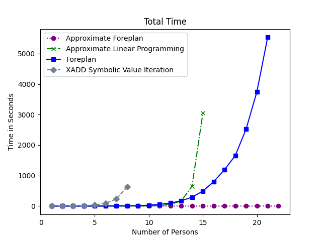
Figure 2: Runtime of (Approximate) Foreplan, ALP and XADD Symbolic Value Iteration on the epidemic example for up to 22 persons with a time limit of two hours.

9 Conclusion

Propositional planning approaches struggle with having numerous indistinct objects and actions on subsets of those objects. While first-order MDPs can cope with numerous objects, they still need to represent actions for each subset individually, resulting in exponentially many actions. In this paper, we present Foreplan, a relational forward planner solving the exponential explosion by lifting the objects: Foreplan groups indistinguishable objects by a representative and carries out calculations on a representative-level. Afterwards, the result is projected to the whole group. Using histograms and focusing only on the number of objects an action is applied to, we effectively reduce the action space from exponential to polynomial in the number of objects. Foreplan allows for answering conditional action queries, enabling iterative planning with constraints. Such queries can be solved in time polynomial in the number of objects. Moreover, Foreplan opens new doors for mechanism design for incentivizing the concurrent actions in the returned policy.

In future work, we aim to develop a hybrid approach combining Foreplan and Golog [23]. With the forward search in Foreplan, we can identify states reachable from the initial state while the backwards search in Golog computes the exact optimal policy. Furthermore, the techniques from Foreplan can be transferred to first-order partially observable MDPs [34].

The research for this paper was funded by the Deutsche Forschungsgemeinschaft (DFG, German Research Foundation) under Germany’s Excellence Strategy – EXC 2176 ’Understanding Written Artefacts: Material, Interaction and Transmission in Manuscript Cultures’, project no. 390893796. The research was conducted within the scope of the Centre for the Study of Manuscript Cultures (CSMC) at Universität Hamburg.

Appendix A Omitted Details

A.1 Examples for the Relational Cost Graph

We illustrate the relational cost graph and later the state representation on a bit more complex setting:

Example 12.

Consider the PRVs $Sick(M)$ and $RemoteWork(M)$ and assume we have a parfactor defined over these two PRVs as well as the PRV $Sick^{\prime}(M)$ for the next state. Then, the relational cost graph consists of two vertices $Sick(M)$ and $RemoteWork(M)$ with an edge between them. Furthermore, we can understand why these two PRVs need to be counted together: A person is (not) sick in the next state dependent on that person being (not) sick and (not) working remote in the current state. We need both values for the correct transition probability.

We now apply the definition of a CRV to Example 12.

Example 13.

The CRV for the clique of $Sick(M)$ and $RemoteWork(M)$ has the structure $\#[Sick(M),RemoteWork(M)]$ and a histogram for that CRV would consist of the four entries $n_{tt}$ for the number of people being sick and working remote, $n_{tf}$ for the number of people sick but not working remote, $n_{ft}$ for the number of people not sick but working remote, and $n_{ff}$ for the number of people not sick and not working remote.

We also provide an example for using our CRVs for counting PRVs defined over different parameters, where regular Counting Random Variables cannot be used:

Example 14.

Suppose we have a parfactor defined over PRVs $Sick(X),Friends(X,Y),Sick(Y)$. The respective CRV has structure $\#[Sick(X),Friends(X,Y),Sick(Y)]$ and we count for each (joint) assignment to the groundings of the PRVs how often this assignment occurs. Assume that $X$ has a domain with only one person $x$ and $Y$ with three, $y_{1}$ to $y_{3}$. Now further assume that $x$ and $y_{1}$ are sick and $x$ is friends with everyone except $y_{2}$. In other words, $x$ is friends with one sick and one healthy person and not friends with a sick person. Thus, the entries in the histogram for $ttt$, $ttf$ and $tft$ are one, while all other ones are zero.

A.2 Proof of Correct State Representation

Theorem.

The representation in Definition 10 is correct.

Proof.

We first lay the foundation for the proof and then continue to show both directions of transformation.

By the definition of a parfactor model $G=\{g_{i}\}$, the full joint probability distribution is

$$P_{G} =\frac{1}{Z}\prod_{f\in gr(G)}f$$ (8)

$$=\frac{1}{Z}\prod_{g\in G}\prod_{f\in gr(g)}f,$$ (9)

with $gr(g)$ referring to the groundings of a parfactor $g$. Without loss of generality, we fix a parfactor $g$. We split the PRVs $\mathcal{B}$ the factor $g$ is defined over into two sets: The set $\mathbf{B}_{in}$ of input PRVs, which contribute to the current state, and the set $\mathbf{B}_{out}$ of output PRVs, which contribute to the next state. We can ignore the set $\mathbf{B}_{out}$, because we only represent the current state and iterate over the next state later in Foreplan.

Given groundings for $g$, we count the occurrences of each assignment to the PRVs in $\mathbf{B}_{in}$. We split the counts into different CRVs according to Definition 10.

Given a state in CRVs, we have to instantiate all possible groundings respecting the current state representation. The PRVs in $\mathbf{B}_{in}$ are possibly split across different CRVs. We can combine any grounding of the PRVs in the different sets, as these PRVs do not share a parameter. ∎

A.3 Calculating Transition Probabilities

In this section, we show how Foreplan calculates the transition probabilities for the constraints in the linear program in Equation 2. Foe each state and action combination, Foreplan generates one constraint. Within this constraint, a sum is taken over all future states. We show how to calculate the required $P(s^{\prime}\mid s,a)$ for given state $s$, action $a$ and next state $s^{\prime}$. We assume that we have one parfactor per PRV in the next state.

Since the transition function is factored, Foreplan calculates the probability of each PRV in the next state separately. Thus, we only need to describe how Foreplan calculates $P(s_{j}^{\prime}\mid s,a)$ for a given current state, given action and given parfactor for state variable $s_{j}^{\prime}$ in the next state. In short, Foreplan first computes the state representation for the current and next state zoomed in at the given parfactor and second iterates over all possible transitions, summing their probabilities. We describe the two steps in more detail.

First, Foreplan computes the state representation only for the input PRVs (including the action PRV) of the parfactor from the given state representation and for the output PRV. Depending on the intertwinedness of the parfactors, the computation is just an extraction or summing out unneeded PRVs from the state representation. At the end of this step, Foreplan has a CRV for the input PRVs and another one for the output CRV for the parfactor.

Let us fix an order the buckets of the input CRV and denote the counts in each bucket by $k_{i},i=1,\dots,n$, where $n$ is the number of buckets.

In the second step, Foreplan iterates over all possible transitions, where one transition specifies transition counts $t_{i},i=1,\dots n$. The transition count $0\leq t_{i}\leq k_{i}$ specifies the number of objects transitioning from bucket $i$ to the true-assignment of the output CRV, $k_{i}-t_{i}$ to the false-assignment, respectively. Since the next state is given, the sum over the $t_{i}$ must be exactly the number of true-assignments in the output CRV. For a fixed transition, Foreplan calculates the probability $P_{t_{i},k_{i}}$ of a fixed bucket $i$ by

$$P_{t_{i},k_{i}}=\binom{k_{i}}{t_{i}}\cdot\phi_{i\to true}^{t_{i}}\cdot\phi_{i\to false}^{k_{i}-t_{i}},$$ (10)

where $\phi_{i\to true}$ denotes the probability for transitioning from bucket $i$ to $true$ and $\phi_{i\to false}$ for the transition to $false$. Both probabilites can be looked-up in the parfactor. For a parfactor for the output PRV $s_{j}$, the computation is thus

$$P(s_{j}\mid s,a)=\sum_{(t_{i})_{i}}\prod_{i}P_{t_{i},k_{i}},$$ (11)

where the sum $\sum_{(t_{i})_{i}}$ goes over all possible transitions.

We illustrate Equation 11 with our running example:

Example 15.

We show how to calculate the probability of the PRV $Travel$. Let us denote the number of persons travelling in the current state by $x$, the number of persons travelling in the next state by $x^{\prime}$, the number of persons travelling and restricted from travelling by $a_{1}$ and the number of persons not travelling and restricted from travelling by $a_{2}$. Then, the sum in Equation 11 goes over all $t_{1},t_{2},t_{3},t_{4}\geq 0$ with

$$t_{1}+t_{2}+t_{3}+t_{4} =x^{\prime},$$ (12)

$$t_{1} \leq a_{1},$$ (13)

$$t_{2} \leq x-a_{1},$$ (14)

$$t_{3} \leq a_{2},$$ (15)

$$t_{4} \leq m-x-a_{2},$$ (16)

where $m$ is the number of persons in our example. We denote by $\phi(travel^{\prime},travel,restrict)$ the probability of a person travelling in the next state given that person is currently (not) travelling and (not) being restricted from travelling. Then, the values $P_{t_{i},k_{i}}$ are calculated by

$$P_{t_{1},a_{1}} =\binom{a_{1}}{t_{1}}\cdot\phi(t,t,t)^{t_{1}}\cdot\phi(f,t,t)^{a_{1}-t_{1}}$$ (17)

$$P_{t_{2},x-a_{1}} =\binom{x-a_{1}}{t_{2}}\cdot\phi(t,t,f)^{t_{2}}\cdot\phi(f,t,f)^{x-a_{1}-t_{2}}$$ (18)

$$P_{t_{3},a_{2}} =\binom{a_{2}}{t_{3}}\cdot\phi(t,f,t)^{t_{3}}\cdot\phi(f,f,t)^{a_{2}-t_{3}}$$ (19)

$$P_{t_{4},m-x-a_{2}} =\binom{m-x-a_{2}}{t_{4}}\cdot\phi(t,f,f)^{t_{4}}$$

$$\quad\quad\cdot\phi(f,f,f)^{m-x-a_{2}-t_{4}}.$$ (20)

A.4 Example of Removing a Maximum Operator

Let us briefly illustrate the step of removing the maximum operator. The removal is a two-phase process. In a first phase, ALP eliminates the variables and in a second phase, ALP generates the constraints for the linear programm along the elimination sequence. Suppose we have the function

$$F=\max_{x_{1},x_{2}}f_{1}(x_{1})+f_{2}(x_{1},x_{2})+f_{3}(x_{2})$$ (21)

in a linear program, e.g., $a\geq F$ or $a=F$, where $a\in\mathbb{R}$ or $a$ as a linear program variable. We start with the first phase. ALP eliminates $x_{1}$ by replacing $f_{1}$ and $f_{2}$ by a new function

$$e_{1}(x_{2})=\max_{x_{1}}f_{1}(x_{1})+f_{2}(x_{1},x_{2}).$$ (22)

ALP eliminates $x_{2}$ by replacing $e_{1}$ and $f_{3}$ by a new function

$$e_{2}=\max_{x_{2}}e_{1}(x_{2})+f_{3}(x_{2}).$$ (23)

Note that $e_{2}$ has an empty scope and evaluates therefore to a number. We continue with the second phase, in which ALP translates the elimination sequence into linear program constraints: In the linear program, ALP adds helping variables and constraints to enforce the maxima in the different terms [16]. For each function $e$ with domain $Z$, ALP adds the variables $u_{z}^{e}$ for each assignment $z$ to $Z$. The variable $u_{z}^{e}$ is supposed to yield the value of $e(z)$. For the initial functions $f_{i}$, in our case $f_{1}$, $f_{2}$, $f_{3}$, ALP simply adds $u_{z}^{f_{i}}=f_{i}(z)$ to the constraints of the linear program. Suppose we got the function $e(z)=\max_{x}e_{i}$ when eliminating some variable $x$. ALP then adds the constraints

$$u_{z}^{e}\geq\sum_{i}u_{(z,x)}^{e_{i}}\ \forall z,x.$$ (24)

For $e_{2}$, the generated constraints would be

$$u^{e_{2}}\geq u_{x_{2}}^{e_{1}}+u_{x_{2}}^{f_{3}}$$ (25)

for all possible values of $x_{2}$. We are interested in keeping the number of added constraints small, which is the aim of VE.

A.5 More Runtime Theorems for Approximate Foreplan

We first define the total relational cost graph:

Definition 22 (Total Relational Cost Graph).

The total relational cost graph for a solution environment for an rfMDP contains a vertex for each (P)RV. Two vertices are connected by an edge if they occur together in a function or parfactor.

By definition, the total relational cost graph is a supergraph for all graphs of interest for the runtime complexity:

Theorem 23.

The following graphs are each subgraphs of the total relational cost graph:

1. relational cost graph

2. the cost network for each maximum constraint in Approximate Foreplan

Proof.

For both cases, we show that the total relational cost graph contains more vertices and edges than the respective definition requires. Thus, we can remove the superfluos vertices and edges to arrive at the respective subgraph.

We start with the relational cost graph. By Definition 8, the relational cost graph has a vertex for each PRV and an edge between two PRVs if they share a logvar and occur together in a parfactor, a parameterized local reward function, or a basis function. In particular, all these vertices and edges are introduced in the total relational cost graph too, when we connect two vertices once the corresponding PRVs occur together in a parfactor. We may add more edges than for the relational cost graph as we ignore the share a logvar condition.

We continue with the cost network for each maximum constraint. Let us take an arbitrary maximum constraint. The cost network consists of vertices for each variable appearing in the constraint and connects two vertices with an edge if the corresponding variables appear together in the same function. Thus, the total relational cost graph contains these edges too, as the respective variables occur together in a function. ∎

Since the induced width is the same as the treewidth minus one, we can give some more bounds:

Theorem 24.

If the total relational cost graph for an rfMDP has bounded treewidth, Approximate Foreplan runs in time polynomial in the number of objects of the rfMDP.

Proof.

By Theorem 23, the relational cost graph is a subgraph of the total relational cost graph. As a subgraph can have the treewidth of the supergraph at most [22], the treewidth of the relational cost graph is bounded. And if a graph has bounded treewidth, it also has bounded clique number, which is our $w$ [22]. Thus, Theorem 17 follows, leaving only the induced width of each cost network.

By Theorem 23, each cost network is a subgraph of the total relational cost graph. The treewidth of each cost network is bounded by the treewidth of the total relational cost graph. As the induced width equals the treewidth minus one, it is bound, leaving no variable with exponential influence. ∎

A.6 Proof of Approximation Guarantee

We now provide the proof that Approximate Foreplan and ALP yield the same results on rfMDPs:

Theorem.

Given an rfMDP $R$, Approximate Foreplan and ALP are equivalent on $R$ and the grounded version of $R$, respectively.

Proof.

We first prove that the basis functions and backprojections evaluate to the same terms. Then, we investigate the setup of the linear programs.

The lifted basis functions accumulate multiple grounded ones. Evaluating a lifted basis function yields the same result as summing the grounded basis functions. For the backprojections, the case is very similar. Evaluating the lifted backprojections as in Definition 16 yields the same result as summing all grounded backprojections, because the objects grouped through PRVs are indistinguishable and share the same transition probabilities. Since we sum over all backprojections and basis functions in the linear program, the equivalence of the sums suffices.

For the linear program, we start with the objective function and continue with the constraints. The objective function used in Approximate Foreplan groups multiple grounded basis functions, which are used in ALP, together in one lifted basis function. Therefore, if we denote the weights in ALP by $\alpha^{\prime}_{i}$, we have the weights $\alpha_{i}=n_{i}\cdot\alpha^{\prime}_{i}$ for Foreplan, where $n_{i}$ stands for the number of grouped basis functions. Since the grouped basis functions are indistinguishable, the weights used in Approximate Foreplan are evenly distributed in ALP. Next, we have the constraints. Since the backprojections and basis functions in Approximate Foreplan evaluate to the same terms as the grounded functions in ALP, each individual constraint is correct. Furthermore, by Theorem 11, Approximate Foreplan covers the whole action space. ∎

A.7 Evaluation

Figure 3 shows the runtime of (Approximate) Foreplan, ALP and XADD Symbolic Value Iteration with a time limit of two hours. The flattening of the runtimes of Foreplan backs our theoretical result in Theorem 15, highlighting that the runtime is indeed not exponential, but rather polynomial, in the number of persons. Moreover, with Approximate Foreplan, we can solve the epidemic example for 164 persons in approximately $2.288$ seconds, which is faster than ALP on 15 persons with approximately $3.045$ seconds and Foreplan on 21 persons with approximately $5.534$ seconds.

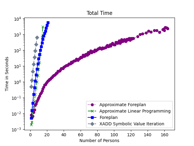
Figure 3: Runtime (logscale) of (Approximate) Foreplan, ALP and XADD Symbolic Value Iteration on the epidemic example with a time limit of two hours and a memory limit of 16 GB. Only runs within these limits are shown.

Appendix B Walkthrough of Approximate Foreplan

We describe in this section how we can solve Example 3 with Approximate Foreplan. We first model the example formally and find the state representation. Afterwards, we precompute the backprojections and instantiate the linear program.

B.1 Modeling the Small Town

We model the setting in Example 3. The town population consists of three people. We refer to Figure 1 for the transition model. We define the parfactors $f_{1}$ and $f_{2}$ according to Tables 1 and 2.

$Travel(M)$	$Restrict(M)$	$Travel^{\prime}(M)$
0	0	0.2
0	1	0.1
1	0	0.9
1	1	0.5

Table 1: Transition probabilities for each person giving the probability of travelling in the next timestep given whether the person is currently travelling and being restricted.

$Sick(M)$	$Epidemic$	$Sick^{\prime}(M)$
0	0	0.2
0	1	0.8
1	0	0.4
1	1	0.6

Table 2: Transition probabilities for each person giving the probability of being sick in the next timestep given whether the person is currently sick and there is an epidemic.

The mayor can restrict an arbitrary subset of the towns population from travelling. The local reward functions are $R_{1}(Sick(M))$ and $R_{2}(Travel(M))$, each for each person of the towns population. The function $R_{1}(Sick(M))$ evaluates to $1$ if the person is not sick and to $-1$ if the person is sick (c.f. Example 5):

$$R_{1}(Sick(M))=\begin{cases}-1,&Sick(M)\\ 1,&\lnot Sick(M)\end{cases}$$ (26)

The function $R_{2}(Travel(M))$ evaluates to $2$ if the person is travelling and to $0$ otherwise:

$$R_{2}(Travel(M))=\begin{cases}2,&Travel(M)\\ 0,&\lnot Travel(M)\end{cases}$$ (27)

We set the discount factor $\gamma=0.9$. For choosing the basis functions, we go with the ones in Example 10, that is, $h_{0}=1$, $h_{1}=R_{1}$ and $h_{2}=R_{2}$.

B.2 State Space Representation

For using Approximate Foreplan, we first build the relational cost graph to find the state space representation. Afterwards, we can modify the actions to be compatible with the state space representation. The relational cost graph contains two vertices, $Sick(M)$ and $Travel(M)$, because these are the only PRVs in the example. The relational cost graph does not contain any edge, because the two PRVs do not occur together in a parfactor, reward or basis function. Thus, the vertices $Sick(M)$ and $Travel(M)$ each are a clique of size one. Therefore, the state space representation contains two histograms along the value of the propositional random variable $Epidemic$. More formally, the state space representation is $([Sick(M)],[Travel(M)],Epidemic)$ (c.f. Example 8).

For the action $Restrict(M)$, the mayor no longer needs to specify on which person(s) she applies the travel ban(s) on, but has to define how many persons currently (not) travelling receive a travel restriction. Thus, the mayor needs to define the action histogram $[Travel(M),Restrict(M)]$ giving the numbers of people (not) travelling that are (not) restricted from travelling (c.f. Example 9).

B.3 Computing Backprojections

The first step of Foreplan is the precomputation of the backprojections. The backprojections are generally defined as

$$g_{i}^{a}(x)=\sum_{x^{\prime}}P(x^{\prime}\mid x,a)\cdot h_{i}(x^{\prime}),$$ (28)

where $x^{\prime}$ are the parameters of $h_{i}$, $x$ are the parents of $x$ in the transition model and $a$ is the selected action. For abbreviation, we use $S(M)$ for $Sick(M)$, $R(M)$ for $Restrict(M)$, $T(M)$ for $Travel(M)$ and $Epi$ for $Epidemic$ in this subsection. We start with the backprojection of $h_{0}=1$:

$$g_{0}^{a}(x)=\sum_{x^{\prime}}P(x^{\prime}\mid x,a)\cdot h_{0}(x)=1\cdot\sum_{x^{\prime}}P(x^{\prime}\mid x,a)=1.$$ (29)

Next, we backproject $h_{1}(Sick(M))$. Note that $Sick^{\prime}(M)$ is independent of the action in the transition model. Thus, the backprojection is independent of $a$:

$$\begin{split}g_{1}(S(M),&Epi)=\\ &\sum_{x^{\prime}\in\{t,f\}}P(S^{\prime}(M)=x^{\prime}\mid S(M),epi)\cdot h_{1}(x^{\prime})\end{split}$$ (30)

We plug the probabilities from Table 2 in and receive

$$g_{1}(true,true) =0.6\cdot(-1)+0.4\cdot 1 =- 0.2,$$ (31)

$$g_{1}(true,false) =0.4\cdot(-1)+0.6\cdot 1 = 0.2,$$ (32)

$$g_{1}(false,true) =0.8\cdot(-1)+0.2\cdot 1 =- 0.6,$$ (33)

$$g_{1}(false,false) =0.2\cdot(-1)+0.8\cdot 1 = 0.6.$$ (34)

The backprojection of $h_{2}$ is a bit more complex, as it includes the action. The general backprojection of $h_{2}$ is given by

$$\begin{split}g_{2}^{R(M)}&(T(M))=\\ &\sum_{x^{\prime}\in\{t,f\}}P(T^{\prime}(M)=x^{\prime}\mid T(M),R(M))\cdot h_{2}(x^{\prime}).\end{split}$$ (35)

We distinguish the two cases $R(M)=false$ and $R(M)=true$. We start with the first one, which leads to:

$$g_{2}^{f}(t) =\sum_{x^{\prime}\in\{t,f\}}P(T^{\prime}(M)=x^{\prime}\mid T(M)=t,R(M)=f)$$ (36)

$$=9\cdot h_{2}(t)+1\cdot h_{2}(f)=9\cdot 2$$

$$=8$$

and

$$g_{2}^{f}(f) =\sum_{x^{\prime}\in\{t,f\}}P(t^{\prime}(P)=x^{\prime}\mid T(M)=f,R(M)=f)$$ (37)

$$=2\cdot h_{2}(t)+8\cdot h_{2}(f)=2\cdot 2$$

$$=4.$$

We continue with $R(M)=true$, leading to

$$g_{2}^{t}(t) =\sum_{x^{\prime}\in\{t,f\}}P(T^{\prime}(M)=x^{\prime}\mid T(M)=t,R(M)=t)$$ (38)

$$=5\cdot h_{2}(t)+5\cdot h_{2}(f)=5\cdot 2$$

$$=1$$

and

$$g_{2}^{t}(f) =\sum_{x^{\prime}\in\{t,f\}}P(T^{\prime}(M)=x^{\prime}\mid T(M)=f,R(M)=t)$$ (39)

$$=1\cdot h_{2}(t)+9\cdot h_{2}(f)=1\cdot 2$$

$$=2.$$

B.4 Instantiation of Linear Program

The second step of Approximate Foreplan is to instantiate the linear program. The linear program has three variables $w_{1}$, $w_{2}$ and $w_{3}$. The objective function is to minimize $\sum_{i=1}^{3}\alpha_{i}w_{i}$, with $\alpha_{i}$ being the relevance weights. We have one constraint for each possible action $a$:

$$0\geq \max_{x_{1},x_{2},x_{3}}\{3-2\cdot x_{1}+2\cdot x_{2}+w_{0}\cdot(9\cdot 1-1)$$ (40)

$$+w_{1}\cdot(9\cdot G_{1}(x_{1},x_{3})-H_{1}(x_{1}))$$

$$+w_{2}\cdot(9\cdot G_{2}^{a}(x_{2})-H_{2}(x_{2}))\},$$

where $x_{1},x_{2}\in\{0,1,2,3\}$ specify the number of persons being sick and travelling, respectively. The variable $x_{3}$ is Boolean and stores the truth value of $Epidemic$. With $G_{i}$ and $H_{i}$ we denote the lifted computation of $g_{i}$ and $h_{i}$. In the following, we write the lifted computation in terms of $x_{i}$ and $g_{i}$ or $h_{i}$. In the remainder of this subsection, we show the complete constraint generation for the linear program for one example action. We omit all other actions because of limited insights compared to one example instantiation and constraint generation. We show the constraint generation for the action of restricting nobody. We start with writing the constraint tailored to this setting and directly computing the value of basis functions and their backprojections lifted:

$$0\geq \max_{x_{1},x_{2},x_{3}}\{3-2x_{1}+2x_{2}-1w_{0}$$ (41)

$$+w_{1}\cdot(x_{1}\cdot 9\cdot g_{1}(t,x_{3})-x_{1}\cdot h_{1}(t))$$

$$+w_{1}\cdot((3-x_{1})\cdot 9\cdot g_{1}(f,x_{3})-(3-x_{1})\cdot h_{1}(f))$$

$$+w_{2}\cdot(x_{2}\cdot 9\cdot g_{2}^{f}(t)-x_{2}\cdot h_{2}(t))$$

$$+w_{2}\cdot((3-x_{2})\cdot 9\cdot g_{2}^{f}(f)-(3-x_{2})\cdot h_{2}(f))\}.$$

We continue with introducing functions to save steps later in variable elimination and constraint generation. We define four functions with different parameters, each collecting the respective terms:

$$0\geq\max_{x_{1},x_{2},x_{3}}\{f_{1}(x_{1})+f_{2}(x_{2})+f_{3}(x_{1},x_{3})+f_{4}\},$$ (42)

with

$$f_{1}(x_{1}) =3-2x_{1}-w_{1}x_{1}h_{1}(t)-w_{1}\cdot(3-x_{1})\cdot h_{1}(f)$$ (43)

$$f_{2}(x_{2}) =2x_{2}+w_{2}\cdot(x_{2}\cdot 0.9\cdot g_{2}^{f}(t)-x_{2}h_{2}(t))$$ (44)

$$\quad\quad+w_{2}\cdot((3-x_{2})\cdot 0.9\cdot g_{2}^{f}(f))$$

$$f_{3}(x_{1},x_{3}) =0.9w_{1}\cdot(x_{1}g_{1}(t,x_{3})+(3-x_{1})\cdot g_{1}(f,x_{3}))$$ (45)

$$f_{4} =-0.1w_{0}$$ (46)

The only task we are left with is to remove the maximum operator. For that, we describe the two phases, variable elimination and constraint generation, in two different subsections.

B.4.1 Variable Elimination

We first eliminate $x_{2}$, leading to

$$0\geq\max_{x_{1},x_{3}}\{f_{1}(x_{1})+e_{1}+f_{3}(x_{1},x_{3})+f_{4}\},$$ (47)

with

$$e_{1}=\max_{x_{2}}f_{2}(x_{2}).$$ (48)

Next, we eliminate $x_{1}$:

$$0\geq\max_{x_{3}}\{e_{2}(x_{3})+e_{1}+f_{4}\},$$ (49)

with

$$e_{2}(x_{3})=\max_{x_{1}}f_{1}(x_{1})+f_{3}(x_{1},x_{3}).$$ (50)

Last, we eliminate $x_{3}$:

$$0\geq e_{1}+e_{3}+f_{4},$$ (51)

with

$$e_{3}=\max_{x_{3}}e_{2}(x_{3}).$$ (52)

B.4.2 Constraint Generation

We generate the constraints along the elimination order of the previous subsection. All the constraints listed in this subsection together replace the single constraint in Equation 40 for our example action of restricting nobody. We start with the constraints for the functions $f_{i}$ containing $w_{i}$s and continue with the functions $e_{i}$ obtained by eliminating variables:

$f_{1}(x_{1})$

$$u_{0}^{f_{1}} =3-3w_{1}$$ (53)

$$u_{1}^{f_{1}} =3-2+w_{1}-2w_{1}=1-w_{1}$$ (54)

$$u_{2}^{f_{1}} =3-4+2w_{1}-w_{1}=-1+w_{1}$$ (55)

$$u_{3}^{f_{1}} =3-6+3w_{1}=-3+3w_{1}$$ (56)

$f_{2}(x_{2})$

$$u_{0}^{f_{2}} =w_{2}\cdot(3\cdot 0.9\cdot 0.4)=3.1w_{2}$$ (57)

$$u_{1}^{f_{2}} =2+w_{2}\cdot(1\cdot 0.9\cdot 1.8-1.2)+w_{2}\cdot(2\cdot 0.9\cdot 0.4)$$

$$=2+0.34w_{2}$$ (58)

$$u_{2}^{f_{2}} =4+w_{2}\cdot(2\cdot 0.9\cdot 1.8-2\cdot 2)+w_{2}\cdot(1\cdot 1.9\cdot 0.4)$$

$$=4-0.04w_{2}$$ (59)

$$u_{3}^{f_{2}} =6+w_{2}\cdot(3-0.9\cdot 1.8-3\cdot 2)=6-1.14w_{2}$$ (60)

$f_{3}(x_{1},x_{3})$

$$u_{00}^{f_{3}} =w_{1}\cdot 3\cdot 0.9\cdot 0.6=1.62w_{1}$$ (61)

$$u_{01}^{f_{3}} =-1.62w_{1}$$ (62)

$$u_{10}^{f_{3}} =w_{1}\cdot 1\cdot 0.9\cdot 0.2+w_{1}\cdot 2\cdot 0.9\cdot 0.6=1.26w_{1}$$ (63)

$$u_{11}^{f_{3}} =-1.26w_{1}$$ (64)

$$u_{20}^{f_{3}} =w_{1}\cdot 2\cdot 0.9\cdot 0.2+w_{1}\cdot 1\cdot 0.9\cdot 0.6=0.9w_{1}$$ (65)

$$u_{21}^{f_{3}} =-0.9w_{1}$$ (66)

$$u_{30}^{f_{3}} =w_{1}\cdot 3\cdot 0.9\cdot 0.2=0.54w_{1}$$ (67)

$$u_{31}^{f_{3}} =-0.54w_{1}$$ (68)

$f_{4}$

$$u^{f_{4}}=-0.1w_{0}$$ (69)

$e_{1}$

$$u^{e_{1}} \geq u_{0}^{f_{2}}$$ (70)

$$u^{e_{1}} \geq u_{1}^{f_{2}}$$ (71)

$$u^{e_{1}} \geq u_{2}^{f_{2}}$$ (72)

$$u^{e_{1}} \geq u_{3}^{f_{2}}$$ (73)

$e_{2}(x_{3})$

$$u_{0}^{e_{2}} \geq u_{0}^{f_{1}}+u_{00}^{f_{3}}$$ (74)

$$u_{0}^{e_{2}} \geq u_{1}^{f_{1}}+u_{10}^{f_{3}}$$ (75)

$$u_{0}^{e_{2}} \geq u_{2}^{f_{1}}+u_{20}^{f_{3}}$$ (76)

$$u_{0}^{e_{2}} \geq u_{3}^{f_{1}}+u_{30}^{f_{3}}$$ (77)

$$u_{1}^{e_{2}} \geq u_{0}^{f_{1}}+u_{01}^{f_{3}}$$ (78)

$$u_{1}^{e_{2}} \geq u_{1}^{f_{1}}+u_{11}^{f_{3}}$$ (79)

$$u_{1}^{e_{2}} \geq u_{2}^{f_{1}}+u_{21}^{f_{3}}$$ (80)

$$u_{1}^{e_{2}} \geq u_{3}^{f_{1}}+u_{31}^{f_{3}}$$ (81)

$e_{3}$

$$u^{e_{3}} \geq u_{0}^{e_{2}}$$ (82)

$$u^{e_{3}} \geq u_{1}^{e_{2}}$$ (83)

Final Constraint

In the end, we add the final constraint

$$0\geq u^{e_{1}}+u^{e_{3}}+u^{f_{4}}$$ (84)

due to the introduction of our helper functions $f_{i}$.

B.4.3 Solving the Linear Program

After having generated all constraints for all actions, the linear program is fed into a solver to compute a solution. The template for the linear program looks like this:

$$\begin{array}[]{ll@{}}\text{Variables:}&w_{1},w_{2},w_{3}\ ;\\ \text{Minimize:}&\alpha_{1}w_{1}+\alpha_{2}w_{2}+\alpha_{3}+w_{3}\ ;\\ \text{Subject to:}&\forall a\in A:\\ &\text{set of constraints generated like in Section~\ref{apx:lp:constraint-generation}}.\\ \end{array}$$ (85)

References

- Apsel and Brafman [2011] U. Apsel and R. I. Brafman. Extended lifted inference with joint formulas. In Proceedings of the 27th Conference on Uncertainty in Artificial Intelligence, pages 11–18, 2011.
- Bellman [1957] R. Bellman. Dynamic programming. Princeton University Press, 1957.
- Bernstein et al. [2002] D. S. Bernstein, R. Givan, N. Immerman, and S. Zilberstein. The complexity of decentralized control of Markov decision processes. Mathematics of operations research, 27(4):819–840, 2002.
- Boutilier et al. [2000] C. Boutilier, R. Dearden, and M. Goldszmidt. Stochastic dynamic programming with factored representations. Artificial intelligence, 121(1-2):49–107, 2000.
- Boutilier et al. [2001] C. Boutilier, R. Reiter, and B. Price. Symbolic dynamic programming for first-order MDPs. In Proceedings of the Seventeenth International Joint Conference on Artificial Intelligence, volume 1, pages 690–700, 2001.
- Braun et al. [2022] T. Braun, M. Gehrke, F. Lau, and R. Möller. Lifting in multi-agent systems under uncertainty. In Proceedings of the Thirty-Eighth Conference on Uncertainty in Artificial Intelligence, pages 233–243, 2022.
- Corrêa and De Giacomo [2024] A. B. Corrêa and G. De Giacomo. Lifted planning: Recent advances in planning using first-order representations. In Proceedings of the 33rd International Joint Conference on Artificial Intelligence, pages 8010–8019, 2024.
- de Farias and Van Roy [2003] D. P. de Farias and B. Van Roy. The linear programming approach to approximate dynamic programming. Operations Research, 51(6):850–865, 2003.
- De Raedt et al. [2016] L. De Raedt, K. Kersting, S. Natarajan, and D. Poole. Statistical relational artificial intelligence: Logic, probability, and computation. Synthesis lectures on artificial intelligence and machine learning, 10(2):1–189, 2016.
- Dean et al. [1997] T. Dean, R. Givan, and S. Leach. Model reduction techniques for computing approximately optimal solutions for Markov decision processes. In Proceedings of the Thirteenth conference on Uncertainty in Artificial Intelligence, pages 124–131, 1997.
- Dechter [1999] R. Dechter. Bucket elimination: A unifying framework for reasoning. Artificial Intelligence, 113(1-2):41–85, 1999.
- d’Epenoux [1960] F. d’Epenoux. Sur un probleme de production et de stockage dans l’aléatoire. Revue Française de Recherche Opérationelle, 14(3-16):4, 1960.
- Gehrke et al. [2019a] M. Gehrke, T. Braun, and R. Möller. Lifted temporal maximum expected utility. In Advances in Artificial Intelligence, pages 380–386, 2019a.
- Gehrke et al. [2019b] M. Gehrke, T. Braun, R. Möller, A. Waschkau, C. Strumann, and J. Steinhäuser. Lifted maximum expected utility. In Artificial Intelligence in Health, pages 131–141, 2019b.
- Givan et al. [2003] R. Givan, T. Dean, and M. Greig. Equivalence notions and model minimization in Markov decision processes. Artificial Intelligence, 147(1-2):163–223, 2003.
- Guestrin et al. [2003] C. Guestrin, D. Koller, R. Parr, and S. Venkataraman. Efficient solution algorithms for factored MDPs. Journal of Artificial Intelligence Research, 19:399–468, 2003.
- Huangfu and Hall [2018] Q. Huangfu and J. J. Hall. Parallelizing the dual revised simplex method. Mathematical Programming Computation, 10(1):119–142, 2018.
- Jeong et al. [2022] J. Jeong, P. Jaggi, A. Butler, and S. Sanner. An exact symbolic reduction of linear smart Predict+Optimize to mixed integer linear programming. In Proceedings of the 39th International Conference on Machine Learning, volume 162, pages 10053–10067, 2022.
- Kaelbling et al. [1998] L. P. Kaelbling, M. L. Littman, and A. R. Cassandra. Planning and acting in partially observable stochastic domains. Artificial intelligence, 101(1-2):99–134, 1998.
- Kersting [2012] K. Kersting. Lifted probabilistic inference. In Proceedings of the 20th European Conference on Artificial Intelligence, pages 33–38, 2012.
- Koller and Parr [1999] D. Koller and R. Parr. Computing factored value functions for policies in structured MDPs. In Proceedings of the Sixteenth International Joint Conference on Artificial Intelligence, volume 2, 1999.
- Koster et al. [2002] A. Koster, H. Bodlaender, and C. van Hoesel. Treewidth: computational experiments. WorkingPaper 001, METEOR, Maastricht University School of Business and Economics, Jan. 2002.
- Levesque et al. [1997] H. J. Levesque, R. Reiter, Y. Lespérance, F. Lin, and R. B. Scherl. GOLOG: A logic programming language for dynamic domains. The Journal of Logic Programming, 31(1-3):59–83, 1997.
- Niepert and Van den Broeck [2014] M. Niepert and G. Van den Broeck. Tractability through exchangeability: A new perspective on efficient probabilistic inference. In Proceedings of the AAAI Conference on Artificial Intelligence, volume 28, pages 2467–2475, 2014.
- Papadimitriou and Tsitsiklis [1987] C. H. Papadimitriou and J. N. Tsitsiklis. The complexity of Markov decision processes. Mathematics of operations research, 12(3):441–450, 1987.
- Poole [2003] D. Poole. First-order probabilistic inference. In Proceedings of the Eighteenth International Joint Conference on Artificial Intelligence, volume 3, pages 985–991, 2003.
- Puterman [1990] M. L. Puterman. Markov decision processes. Handbooks in operations research and management science, 2:331–434, 1990.
- Sanner and Boutilier [2007] S. Sanner and C. Boutilier. Approximate solution techniques for factored first-order MDPs. In Proceedings of the Seventeenth International Conference on Automated Planning and Scheduling, pages 288–295, 2007.
- Sanner and Kersting [2010] S. Sanner and K. Kersting. Symbolic dynamic programming for first-order POMDPs. In Proceedings of the AAAI Conference on Artificial Intelligence, volume 24, pages 1140–1146, 2010.
- Taghipour [2013] N. Taghipour. Lifted probabilistic inference by variable elimination. PhD dissertation, KU Leuven, 2013.
- Taghipour et al. [2013] N. Taghipour, D. Fierens, J. Davis, and H. Blockeel. Lifted Variable Elimination: Decoupling the Operators from the Constraint Language. Journal of Artificial Intelligence Research, 47:393–439, 2013.
- Taitler et al. [2022] A. Taitler, M. Gimelfarb, S. Gopalakrishnan, M. Mladenov, X. Liu, and S. Sanner. pyrddlgym: From rddl to gym environments. arXiv preprint arXiv:2211.05939, 2022.
- Vaidya [1989] P. Vaidya. Speeding-up linear programming using fast matrix multiplication. In 30th Annual Symposium on Foundations of Computer Science, pages 332–337, 1989.
- Williams et al. [2005] J. D. Williams, P. Poupart, and S. Young. Factored partially observable Markov decision processes for dialogue management. In Proceedings of the 4th IJCAI Workshop on Knowledge and Reasoning in Practical Dialogue Systems, pages 76–82, 2005.
- Zhang and Poole [1994] N. L. Zhang and D. Poole. A simple approach to Bayesian network computations. In Proceedings of the 10th Canadian Conference on AI, pages 171–178, 1994.