Multi-period Mean-Buffered Probability of Exceedance in
Defined Contribution Portfolio Optimization

Abstract

We investigate multi-period mean–risk portfolio optimization for long-horizon Defined Contribution plans, focusing on buffered Probability of Exceedance (bPoE), a more intuitive, dollar-based alternative to Conditional Value-at-Risk (CVaR). We formulate both pre-commitment and time-consistent Mean–bPoE and Mean–CVaR portfolio optimization problems under realistic investment constraints (e.g. no leverage, no short selling) and jump-diffusion dynamics. These formulations are naturally framed as bilevel optimization problems, with an outer search over the shortfall threshold and an inner optimization over rebalancing decisions. We establish an equivalence between the pre-commitment formulations through a one-to-one correspondence of their scalarization optimal sets, while showing that no such equivalence holds in the time-consistent setting. We develop provably convergent numerical schemes for the value functions associated with both precommitment and time-consistent formulations of these mean-risk control problems.

Using nearly a century of market data, we find that time-consistent Mean–bPoE strategies closely resemble their pre-commitment counterparts. In particular, they maintain alignment with investors’ preferences for a minimum acceptable terminal wealth level—unlike time-consistent Mean–CVaR, which often leads to counterintuitive control behaviour. We further show that bPoE, as a strictly tail-oriented measure, prioritizes guarding against catastrophic shortfalls while allowing meaningful upside exposure—making it especially appealing for long-horizon wealth security. These findings highlight bPoE’s practical advantages for long-horizon retirement planning.

Keywords: Mean-risk portfolio optimization, Buffered Probability of Exceedance, Conditional Value-at-Risk, Pre-commitment, Time-consistent

AMS Subject Classification: 91G, 65R20, 93E20, 49M25

1 Introduction

The main objective of this paper is to investigate buffered Probability of Exceedance as a viable alternative risk measure to Conditional Value-at-Risk for multi-period Defined Contribution portfolio optimization.

1.1 Motivation

Saving for and managing wealth throughout retirement remains one of the most critical and challenging financial tasks facing individuals. This challenge is magnified by the global shift from Defined Benefit (DB) to Defined Contribution (DC) pension systems, which places the full burden of investment and longevity risk—the possibility that individuals outlive their retirement savings—on plan participants. In many countries, including Australia, the United States, Canada, and parts of Europe, this shift has led to the emergence of “full-life cycle” DC plans that span several decades, covering both the accumulation (working years) and decumulation (retirement) phases.

Compounding these challenges is the rapid aging of the world’s population [55], together with the current era of rising inflation and economic turbulence, all of which underscore the urgency of prudent lifecycle financial planning. Moreover, low levels of financial literacy further exacerbate long-horizon financial decision-making. Consequently, there is a clear need for risk measures that combine mathematical rigor with intuitive, readily interpretable insights, enabling retail investors—particularly retirees—and DC plan providers to understand, communicate, and manage downside risk within long-horizon portfolio decision-making.

Over the past few decades, a number of risk measures have been proposed for portfolio optimization, with increasing emphasis on left-tail metrics that capture downside risk. In this context, investors typically aim to maximize some notion of reward–such as the expectation of terminal wealth or total withdrawals—while minimizing a measure of risk, leading to so-called “reward–risk” portfolio optimization.

Among the various risk measures proposed, Conditional Value-at-Risk (CVaR), also known as Expected Shortfall, stands out as a natural means of capturing left-tail risk in a portfolio’s wealth outcomes. Specifically, it measures the average of the worst $\alpha$-fraction of wealth outcomes, where $\alpha\in(0,1)$ is a confidence level [50]. Mathematically, CVaR at confidence level $\alpha$ can be expressed through a threshold-based optimization formulation, in which a candidate shortfall threshold variable $W_{a}$ partitions the wealth distribution into its worst $\alpha$-fraction and the remainder. This threshold-based formulation is widely employed in portfolio optimization due to its significant computational advantages [50, 38]. Although CVaR is often defined on losses (making lower values preferable), this paper defines CVaR on terminal wealth so that higher values are desirable.

CVaR has gained considerable popularity in risk management due to its coherent risk properties and its ability to be optimized efficiently using scenario-based linear programs or non-smooth convex optimization methods [50, 31]. As a result, CVaR-based formulations have become standard in institutional portfolio construction and widely adopted in academic research (see, for example, [4, 13, 41, 3, 37, 20] among many other publications). Crucially, CVaR’s focus on left-tail risk is especially relevant for individuals in the accumulation phase—who face the possibility of not achieving sufficient retirement savings—as well as for retirees in the decumulation phase—who risk outliving their wealth—making CVaR a suitable risk measure across the entire retirement lifecycle [24].

Despite CVaR’s widespread adoption in institutional settings and academic research, in our experience, practitioners frequently observe that its probability-based formulation can be opaque to many retail investors, who tend to prefer tangible minimum acceptable terminal wealth levels over an abstract confidence level such as $\alpha$. This observation aligns with broader research documenting widespread gaps in financial literacy, as mentioned earlier, with [35] noting that “across countries, financial literacy is at a crisis level,…individuals have the lowest level of knowledge around the concept of risk, and risk diversification.”

In light of these considerations, the buffered Probability of Exceedance (bPoE) [39, 38] emerges as a risk measure that preserves many of CVaR’s key advantages while offering a more intuitive, dollar-based perspective on minimum acceptable terminal wealth. More specifically, bPoE directly specifies a “disaster level” $D$ in dollar terms and identifies the minimal probability mass in the left tail whose conditional average equals $D$. As with CVaR, we define bPoE on terminal wealth, ensuring that a lower bPoE value corresponds to a more favorable outcome from the investor’s perspective. Conceptually, bPoE can be viewed as the inverse of CVaR: whereas CVaR fixes $\alpha$ and calculates the average wealth in the left-$\alpha$ tail of the distribution, bPoE instead fixes the disaster level $D$ and determines the corresponding probability level [39]. Similar to CVaR, bPoE at a fixed disaster level $D$ can also be expressed through a threshold-based optimization formulation, using a candidate shortfall threshold $W_{o}$ that partitions the terminal wealth distribution into a left-tail with conditional average equal to $D$, and the remainder [39].

To illustrate, consider an investor concerned about their DC account balance falling below $100,000—a level they regard as the minimum acceptable terminal wealth. In a CVaR framework, the investor would first select a probability level $\alpha$ (e.g. 5%) and then compute the average wealth in the worst $\alpha$-fraction of scenarios—an approach that appears detached from the practical concern of falling below a specific dollar-based terminal wealth level. By contrast, bPoE begins by fixing $100,000 as the disaster level $D$ and determines the likelihood that terminal wealth falls into a region whose conditional average equals $100,000. This dollar-based framing naturally addresses the core question: “What is the chance that my retirement wealth falls into a disaster region where the average outcome is only $100,000?”. As a result, bPoE is more intuitive for retail investors and supports clearer communication between DC plan holders and providers.

While CVaR-based frameworks have become standard in portfolio optimization [41, 27, 20], bPoE remains largely unexplored within this domain—despite its promising theoretical properties [39, 44]. A notable exception is the single-period analysis in [44], which derives closed-form expressions for bPoE under certain probability distributions and demonstrates its use in portfolio selection and density estimation. However, to the best of our knowledge, bPoE has not been explored in either discrete- or continuous-time multi-period portfolio optimization settings, where notions of time-consistency and pre-commitment (the latter being inherently time-inconsistent) play a central role in investment decisions. As we shall see, the fixed dollar disaster level $D$ in bPoE not only aligns more naturally with investors’ absolute wealth perspectives, but also offers insights into significant advantages over CVaR in developing time-consistent solutions for multi-period portfolio optimization.

Furthermore, while tail-based reward–risk formulations, such as Mean–CVaR, are well established in theory and increasingly explored in practice, there remains a notable lack of provably convergent numerical methods for computing the value functions of these problems in multi-period settings under realistic market dynamics and investment constraints. This limitation highlights the need for reliable numerical tools that enable the practical adoption of these strategies.

1.2 Background

Broadly speaking, two main approaches have been developed for multi-period mean–risk portfolio optimization: the pre-commitment approach and the time-consistent approach. Pre-commitment strategies are known to exhibit time-inconsistent behavior [9, 11, 10, 8]. Concretely, time-inconsistency means that there exists $0\leq t_{k}<t_{l}<t_{n}\leq T$, where $T$ is the finite investment horizon, such that the optimal decision for time $t_{n}$, computed at $t_{k}$, differs from the optimal decision for the same time $t_{n}$, but computed at a later time $t_{l}$.

A classic illustration of this phenomenon is Mean-Variance optimization, where the variance of the terminal wealth serves as the risk-measure. Because the variance term in the Mean–Variance objective is not separable in the sense of dynamic programming, the Bellman principle cannot be applied, thereby resulting in time-inconsistency [33, 15, 61, 41]. Likewise, CVaR and bPoE are nonlinear risk measures, and hence their associated mean–risk objectives are also non-separable in the sense of dynamic programming.

In contrast, the time-consistent approach enforces an explicit time-consistency constraint that, for any $0\leq t_{k}<t_{l}<t_{n}\leq T$, the optimal control for time $t_{n}$, computed at $t_{l}$, must match the optimal control for the same time $t_{n}$, but computed at earlier time $t_{k}$. Imposing this constraint restores dynamic-programming tractability by making the mean-risk objective satisfy the Bellman principle [6, 52, 51, 20]. However, since time-consistent strategies can be viewed as pre-commitment strategies with an additional constraint, they are generally not globally optimal when evaluated from time zero. The reader is referred to [57] for a broader discussion of the merits and demerits of time-consistent and pre-commitment policies.

Without enforcing time consistency, multi-period portfolio optimization under the pre-commitment framework generally yields strategies that are globally optimal when viewed from time zero, but may not remain optimal as time evolves. This has led many researchers to label pre-commitment strategies as non-implementable. However, in certain specialized settings, the pre-commitment strategy can be reformulated as a time-consistent solution under an alternative objective.

For example, in Mean–Variance optimization, the pre-commitment strategy can be recast as a time-consistent solution under an alternative objective that minimizes quadratic shortfall relative to a fixed wealth target, often referred to as the Mean–Variance–induced utility maximization problem [54]. Likewise, in both continuous-time [41, 27] and multi-period [20] Mean–CVaR portfolio optimization, although pre-commitment strategies are formally time-inconsistent, they can be equivalently viewed at time zero as linear shortfall policies with a fixed wealth threshold—policies that are time-consistent [20]. Therefore, in both cases, the investor has no incentive to deviate from the strategy computed at inception, rendering the pre-commitment solution effectively implementable.

Interestingly, the literature has observed that imposing time-consistency constraints in Mean-CVaR portfolio optimization can lead to undesirable properties in the resulting optimal controls, even under otherwise realistic conditions. In discrete rebalancing settings with no leverage and no short selling, time-consistent Mean-CVaR strategies have been found to be wealth–independent in lump-sum investment scenarios—and only weakly dependent otherwise—thus behaving similarly to deterministic strategies and offering little or no improvement over simple constant-weight strategies [20, 23].

This phenomenon arises because time-consistent Mean-CVaR policies re-optimize the shortfall threshold $W_{a}$ at each rebalancing time based on current wealth, which can vary substantially from earlier wealth levels. Thus, the shortfall threshold $W_{a}$ shifts over time in response to these wide fluctuations. In contrast, as noted earlier, most investors naturally prefer anchoring their investment strategy to a fixed minimum terminal wealth level rather than redefining the shortfall threshold whenever their wealth changes. In fact, [20] states

“At time zero, we have some idea of what we desire as a minimum final wealth. Fixing this shortfall target for all $t>0$ makes intuitive sense.”

Therefore, re-optimizing the shortfall threshold $W_{a}$ across a wide range of possible wealth levels in time-consistent Mean-CVaR solutions can conflict with these absolute goals, leading to strategies that are often viewed as counterintuitive from a practical standpoint. We note that related paradoxes concerning time-consistent Mean–Variance formulations under constraints have also been discussed; see [7] for details.

By contrast, pre-commitment Mean-CVaR formulations, while formally time-inconsistent, adopt a fixed shortfall threshold from inception—thus aligning more closely with the minimum terminal wealth levels that investors typically prefer and delivering more practically appealing outcomes.

1.3 Contributions

While the prevailing narrative in the literature emphasizes that enforcing time-consistency can lead to counterintuitive outcomes, we argue that the choice of risk measure is equally critical in shaping the behavior of time-consistent portfolio strategies. In particular, it is not the imposition of time-consistency itself that causes undesirable outcomes; rather, the behavior of the solution critically depends on how subproblems are re-solved at each state and time step, an aspect that is fundamentally governed by the structure of the risk measure. Unlike its CVaR counterpart, time-consistent Mean-bPoE—anchored by a fixed disaster level $D$—enforces a constrained re-optimization of the bPoE shortfall threshold $W_{o}$ at each time step. Specifically, $W_{o}$ must define a left-tail region whose conditional average equals $D$, thereby limiting how much the threshold can shift in response to wealth fluctuations. As a result, the policy may remain better aligned with an investor’s minimum terminal wealth preferences, thus avoiding the counterintuitive behavior of investment controls often observed in time-consistent formulations.

In response to these observations, this paper sets out to achieve three primary objectives. First, we formulate multi-period Mean–bPoE and Mean–CVaR optimization frameworks under both pre-commitment and time-consistent settings, incorporating realistic investment constraints and modeling assumptions appropriate for long-horizon DC plans. We then develop and analyze a provably convergent numerical scheme to compute the resulting value functions and optimal controls under these frameworks. For illustration, we focus specifically on the accumulation phase. Second, we analyze the mathematical connection between Mean–bPoE and Mean–CVaR strategies, motivated by the fact that these risk measures are inverse to one another, and explore how this duality influences their behaviour under both optimization paradigms. Third, using nearly a century of actual market data, we illustrate the properties of both Mean–bPoE and Mean–CVaR strategies, with particular focus on whether bPoE’s minimum terminal wealth perspective can avoid the counterintuitive control behaviour often observed in time-consistent mean–risk formulations.

The main contributions of this paper are as follows.

• We present both the pre-commitment and time-consistent formulations of multi-period Mean–bPoE and Mean–CVaR portfolio optimization problems using a scalarization approach. For the pre-commitment case, we establish the existence of finite optimal thresholds. Building on this result, we then show that pre-commitment Mean–bPoE and Mean–CVaR formulations can be reformulated as time-consistent target-based portfolio problems, thereby ensuring their implementability.

• We then rigorously establish an equivalence between the pre-commitment Mean–bPoE and Mean–CVaR formulations, in the sense of a one-to-one correspondence between points on their scalarization optimal sets (i.e. efficient frontiers), under appropriately calibrated scalarization parameters, such that each corresponding pair is attained by the same optimal threshold and rebalancing control. As a result, the induced distributions of terminal wealth are identical under both formulations.

  In contrast, we demonstrate that this equivalence does not hold in the time-consistent setting: the time-consistent Mean–bPoE and Mean–CVaR optimal controls exhibit fundamentally different behavior with respect to wealth dependence.

• We develop a unified numerical framework for both pre-commitment and time-consistent multi-period Mean–bPoE and Mean–CVaR formulations, based on monotone numerical integration. To the best of our knowledge, this is the first work to establish convergence of a numerical scheme to the value function for these problems under realistic market dynamics and investment constraints.

• We conduct a comprehensive numerical comparison of Mean–bPoE and Mean–CVaR optimization results, examining the behavior of optimal investment strategies, terminal wealth distributions, and several key performance metrics—including the mean of terminal wealth, CVaR, bPoE, and the 5th, 50th, and 95th percentiles. All numerical experiments use model parameters calibrated to 88 years of inflation-adjusted long-term U.S. market data, enabling realistic conclusions to be drawn.

  We find that pre-commitment Mean–bPoE and its CVaR counterpart yield virtually identical investment outcomes across all comparison metrics, consistent with the theoretical equivalence established earlier. Consequently, pre-commitment Mean–bPoE can be integrated seamlessly into existing Mean–CVaR workflows, allowing institutions to adopt a dollar-based risk measure without altering broader frameworks or results.

• In contrast, time-consistent Mean–bPoE and Mean–CVaR strategies exhibit fundamentally different control behaviour and investment outcomes, consistent with theoretical findings.

  For the same mean of terminal wealth, time-consistent Mean–bPoE outperforms its Mean–CVaR counterpart on nearly all comparison metrics, including CVaR, bPoE, and the 5th and 95th percentiles, while yielding a noticeably lower median. This reflects a key distinction: Mean–CVaR tends to compress the wealth distribution toward the median, whereas Mean–bPoE emphasizes tail performance by prioritizing protection against catastrophic shortfalls while allowing meaningful upside exposure. As a result, bPoE may be especially appealing for investors focused on long-term wealth security rather than distributional tightness.

The remainder of the paper is organized as follows. Section 2 describes the investment setting and the underlying asset dynamics. Section 3 introduces the two risk measures—CVaR and bPoE—and discusses their inverse relationship. In Section 4, we define the scalarization optimal sets for the pre-commitment formulations and examine their key properties. Section 5 establishes the equivalence between pre-commitment Mean–bPoE and Mean–CVaR formulations and discusses their respective implementability under a target-based interpretation. In Section 6, we present the formulations for time-consistent Mean–bPoE and Mean–CVaR, and examine key differences in the behavior of their optimal controls. A unified numerical framework applicable to both settings is developed in Section 7. Section 8 presents and discusses the numerical results. Section 9 concludes the paper and outlines directions for future research.

2 Modelling

2.1 Rebalancing discussion

We consider a portfolio consisting of a risky asset and a risk-free asset. In practice, the risky asset may represent a broad market index, while the risk-free asset could be a bank account. This setup is justified by the observation that a diversified portfolio of various risky assets, such as stocks, can often be approximated by a single broad index. Long-term investors typically focus on strategic asset allocation—determining how much to allocate to different asset classes—rather than selecting individual stocks.

We consider a complete filtered probability space $(\mathcal{S},\mathcal{F},\{\mathcal{F}_{t}\}_{0\leq t\leq T},\mathbb{P})$, where $\mathcal{S}$ is the sample space, $\mathcal{F}$ is a $\sigma$-algebra, $\{\mathcal{F}_{t}\}_{0\leq t\leq T}$ is the filtration over a finite investment horizon $T>0$, and $\mathbb{P}$ is the real-world probability measure. Let $S(t)$ and $B(t)$ respectively denote the amounts invested in the risky and risk-free assets at time $t\in[0,T]$. The total wealth at time $t$ is $W(t)=S(t)+B(t)$. For simplicity, we often write $S_{t}=S(t)$, $B_{t}=B(t)$, and $W_{t}=W(t)$. We also denote by $\{X_{t}\}$, $t\in[0,T]$, where $X_{t}=(S_{t},B_{t})$, the multi-dimensional controlled underlying process, and let $x=(s,b)$ represent a generic state of the system.

We also let $\mathcal{T}$ be the set of $M$ pre-determined, equally spaced, rebalancing times in $[0,T]$:

$$\mathcal{T}=\{t_{m}\mid t_{m}=m\Delta t,\ m=0,\dots,M-1\},\quad\Delta t=T/M,$$ (2.1)

where $t_{0}=0$ is the inception time of the investment. At each rebalancing time $t_{m}\in\mathcal{T}$, the investor first adjusts the portfolio by incorporating a cashflow $q_{m}$, either as a deposit or withdrawal, and then rebalances the portfolio. At time $t_{M}=T$, the portfolio is liquidated (no rebalancing), yielding the terminal wealth $W_{T}$.

For subsequent use, we define the shorthand notation for instants just before and after time $t\in[0,T]$ respectively as:

$$t^{-}=t-\epsilon,\quad\text{ and }\quad t^{+}=t+\epsilon,\quad\text{ where }\epsilon\to 0^{+}.$$

For a generic time-dependent function $f(t)$, we write:

$$f_{m}^{-}=\lim_{\epsilon\to 0^{+}}f(t_{m}-\epsilon),\quad f_{m}^{+}=\lim_{\epsilon\to 0^{+}}f(t_{m}+\epsilon),\quad\text{where }t_{m}\in\mathcal{T}.$$

As noted in [20], DC plan savings are typically held in tax-advantaged accounts, where portfolio rebalancing does not trigger immediate tax liabilities. This includes 401(k) plans in the United States, superannuation funds in Australia, and similar tax-advantaged savings vehicles worldwide. Given this, we assume no taxes in our analysis. In addition, rebalancing occurs infrequently on a fixed schedule, such as annually, reducing trading activity and significantly lowers costs associated with bid-ask spreads, brokerage fees, and market impact; hence, we assume no transaction costs. Given these assumptions, the total wealth at time $t_{m}^{+}$ after incorporating the cashflow $q_{m}$ is given by

$$W_{m}^{+}=W_{m}^{-}+q_{m},\quad t_{m}\in\mathcal{T}.$$ (2.2)

For a rebalancing time $t_{m}\in\mathcal{T}$, we use $u_{m}(\cdot)\equiv u(\cdot)$ to denote the rebalancing control which is the proportion of total wealth allocated to the risky asset. This proportion depends on both the total wealth $W_{m}^{+}$ (including the cashflow) and time $t_{m}$, i.e.

$$u_{m}(\cdot)=u_{m}(W_{m}^{+})=u(W_{m}^{+},t_{m}),\quad\text{where $W_{m}^{+}$ is given by \eqref{eq:cash}}.$$

We denote by $\mathcal{Z}$ the set of all admissible rebalancing controls, i.e. $u_{m}\in\mathcal{Z}$ for every $t_{m}\in\mathcal{T}$. The set $\mathcal{Z}$ is typically determined by investment constraints. To enforce no leverage and no shorting, we impose $\mathcal{Z}=[0,1]$.

Suppose that the investor applies the rebalancing control $u_{m}\in\mathcal{Z}$ at $t_{m}\in\mathcal{T}$, and the system is in state $x=(s,b)$ immediately before rebalancing, i.e. at time $t_{m}^{-}$. Hence, $W_{m}^{-}=s+b$. We let $X_{m}^{+}=(S_{m}^{+},B_{m}^{+})\equiv(S^{+}(s,b,u_{m}),B^{+}(s,b,u_{m}))$ denote the state of the system immediately after applying $u_{m}$. We then have

$$S_{m}^{+} \equiv{{\color[rgb]{0,0,0}{s^{+}(s,b,u_{m})}}}=u_{m}\,W_{m}^{+},\quad\text{and}\quad B_{m}^{+}\equiv{{\color[rgb]{0,0,0}{b^{+}(s,b,u_{m})}}}=\left(1-u_{m})\right)\,W_{m}^{+},$$ (2.3)

$$\qquad\text{ where by \eqref{eq:cash} }W_{m}^{+}=W_{m}^{-}+q_{m}=s+b+q_{m}.$$

Let $\mathcal{A}$ be the set of admissible controls, defined as follows

$$\mathcal{A}=\left\{\,\mathcal{U}=\left\{u_{m}\right\}_{m=0,\ldots,M-1}\big{|}u_{m}\in\mathcal{Z},\text{ for }m=0,\ldots,M-1\right\}.$$ (2.4)

For any rebalancing time $t_{m}$, we define the subset of controls applicable from $t_{m}$ onward as

$$\mathcal{U}_{m} = \left\{\left.u_{m^{\prime}}\ \right|\ u_{m^{\prime}}\in\mathcal{Z},\ m^{\prime}=m,\ldots,M-1\right\}\subseteq\mathcal{U}_{0}\equiv\mathcal{U}.$$ (2.5)

2.2 Underlying dynamics

In practice, real (inflation-adjusted) returns are more relevant to investors than nominal returns [22, 56]. Consequently, we model both the risky and risk-free assets in real terms. All parameters, including the risk-free interest rate, are thus taken to be inflation-adjusted. Given that we focus on relatively long investment horizons (often 20 or 30 years) and that real interest rates tend to be mean-reverting, we assume a constant, continuously compounded real risk-free interest rate $r$.

Between consecutive rebalancing times, the process $\{B_{t}\}$ follows

$$dB_{t} = r\,B_{t}\,dt,\quad t\in[\,t_{m}^{+},\,t_{m+1}^{-}],\quad t_{m}\in\mathcal{T},$$ (2.6)

where $r$ is the constant real risk-free rate. In a discrete setting, the amount invested in the risk-free asset remains constant over $[t_{m}^{+},\,t_{m+1}^{-}]$ and is updated at $t_{m+1}$ to reflect the interest accrued over $[t_{m},\,t_{m+1}]$. Specifically, if the risk-free amount at $t_{m}^{+}$ is $B_{t_{m}^{+}}=b$, it remains at $b$ throughout $[t_{m}^{+},\,t_{m+1}^{-}]$ and is updated to $b\,e^{r\,\Delta t}$ at $t_{m+1}$. Rebalancing then occurs immediately after settlement, i.e. over $[t_{m+1},\,t_{m+1}^{+}]$.

To capture more realistic behavior of the risky asset, we allow for both diffusion and jump components [34]. We let the random variable $\xi$ be the jump multiplier. If a jump occurs at time $t$, the amount invested in the risky asset jumps from $S_{t^{-}}$ to $S_{t}=\xi\,S_{t^{-}}$. We adopt the Kou model [29, 30], in which $\log(\xi)$ follows an asymmetric double-exponential distribution. The probability density function of $\log(\xi)$ is given by

$$\rho(\zeta) = p_{up}\,\eta_{1}\,e^{-\eta_{1}\,\zeta}\,\mathbb{I}_{\{\zeta\geq 0\}}\;+\;(1-p_{up})\,\eta_{2}\,e^{\eta_{2}\,y}\,\mathbb{I}_{\{\zeta<0\}},\quad p_{up}\in[0,1],\ \eta_{1}>1,\ \eta_{2}>0.$$ (2.7)

Between consecutive rebalancing times, in the absence of active control, the process $\{S_{t}\}$ evolves according to the jump-diffusion dynamics:

$$\frac{dS_{t}}{S_{t^{-}}} = \bigl{(}\mu-\lambda\,\kappa\bigr{)}\,dt\;+\;\sigma\,dZ_{t}\;+\;d\Bigl{(}\!\sum_{i=1}^{\pi_{t}}\!(\xi_{i}-1)\Bigr{)},\quad t\in[\,t_{m}^{+},\,t_{m+1}^{-}],\quad t_{m}\in\mathcal{T}.$$ (2.8)

Here, $\mu$ and $\sigma$ are the (inflation-adjusted) drift and instantaneous volatility, respectively, and $\{Z_{t}\}_{t\in[0,T]}$ is a standard Brownian motion. The process $\{\pi_{t}\}_{0\leq t\leq T}$ is a Poisson process with a constant finite intensity rate $\lambda\geq 0$. All jump multiplier $\xi_{i}$ are i.i.d. with the same distribution as random variable $\xi$, and $\kappa=\mathbb{E}[\xi-1]$ is the compensated drift adjustment, where $\mathbb{E}[\cdot]$ is the expectation taken under the real-world measure $\mathbb{P}$. It is further assumed that $\{Z_{t}\}_{t\in[0,T]}$, $\{\pi_{t}\}_{0\leq t\leq T}$, and all $\{\xi_{i}\}$ are mutually independent. Note that GBM dynamics for $\{S_{t}\}$ can be recovered from (2.8) by setting the intensity parameter $\lambda$ to zero.

3 Risk measures

In this and the next sections, we introduce two risk measures, namely CVaR and bPoE, along with their corresponding mean-risk portfolio optimization formulations. For simplicity and clarity, we establish the following notational conventions. A subscript $j\in\{a,o\}$ is used to distinguish quantities related to the CVaR risk measure or CVaR-based formulation ($j=a$) from those corresponding to the bPoE counterparts ($j=o$). Additionally, a superscript “$p$” denotes quantities associated with pre-commitment optimizations, while a superscript “$c$” identifies those related to their time-consistent counterparts.

3.1 Conditional Value-at-Risk

Recalling that $W_{T}$ is the random variable representing terminal wealth, we let $g(w)$ denote its pdf. For a given confidence level $\alpha$, typically $0.01$ or $0.05$, the CVaR of $W_{T}$ at level $\alpha$ is defined as

$$\text{CVaR}_{\alpha}\left(W_{T}\right) = \tfrac{1}{\alpha}\int_{-\infty}^{\text{VaR}_{\alpha}\left(W_{T}\right)}w\ g\left(w\right)dw.$$ (3.1)

Here, $\text{VaR}_{\alpha}(W_{T})$ denotes the Value-at-Risk (VaR) of $W_{T}$ at confidence level $\alpha$, given by

$$\text{VaR}_{\alpha}\left(W_{T}\right) = \left\{\left.w\ \right|\ \mathbb{P}\left[\ W_{T}\leq w\ \right]=\alpha\right\}.$$ (3.2)

That is,

$$\int_{-\infty}^{\text{VaR}_{\alpha}\left(W_{T}\right)}g\left(w\right)dw=\alpha.$$ (3.3)

We can interpret $\text{VaR}_{\alpha}(W_{T})$ as the threshold such that $W_{T}$ falls below this value with probability $\alpha$ [49]. Intuitively, given a pre-specified $\alpha$, $\text{CVaR}_{\alpha}(W_{T})$ represents the average level of $W_{T}$ in the worst $\alpha$-fraction of all possible outcomes, i.e. in the leftmost $\alpha$-quantile of the distribution of $W_{T}$.

As noted in [50], the integral-based definition of $\text{CVaR}_{\alpha}\left(W_{T}\right)$ given in (3.1) often becomes cumbersome when embedded in optimization problems, particularly those involving complex or non-smooth probability distributions of terminal wealth. To address this, [50] shows that $\text{CVaR}_{\alpha}\left(W_{T}\right)$ can be reformulated as a more computationally tractable optimization problem. The key idea in [50] is to introduce a candidate threshold $W_{a}$ that effectively partitions the probability distribution of $W_{T}$ into its lower tail and the remainder. Optimizing over this threshold leads to an equivalent formulation for $\text{CVaR}_{\alpha}\left(W_{T}\right)$:

$$\text{CVaR}_{\alpha}\left(W_{T}\right) = \sup_{W_{a}}\mathbb{E}\left[W_{a}+\tfrac{1}{\alpha}\min\left(W_{T}-W_{a},0\right)\right].$$ (3.4)

We note that the theoretical range of $W_{a}$ coincides with the set of all feasible values for $W_{T}$, which is $[0,\infty)$ under the no-leverage, no-shorting constrain. We denote by $W_{a}^{*}$ the optimal threshold, i.e.

$$W_{a}^{*}\in\mathop{\rm arg\,max}_{W_{a}}\,\mathbb{E}\left[W_{a}+\tfrac{1}{\alpha}\min\left(W_{T}-W_{\alpha},0\right)\right].$$ (3.5)

Because $W_{T}$ is treated here as a gain-oriented variable, the worst outcomes lie in the left tail; hence, the formulation (3.4) employs $\sup(\cdot,\cdot)$ and $\min(\cdot,0)$ (rather than $\max(\cdot,0)$, which is more common in loss-oriented setups). Notably, the optimal threshold $W_{a}^{*}$ that attains the optimum in (3.4) coincides with $\text{VaR}_{\alpha}(W_{T})$ [50].

From a computational standpoint, the threshold-based formulation (3.4) is often more tractable than the integral-based definition (3.1) of $\text{CVaR}_{\alpha}\left(W_{T}\right)$. Therefore, we adopt it for the remainder of this paper.

3.2 Buffered Probability of Exceedance

For a given disaster level $D$, we define the bPoE of the terminal wealth $W_{T}$ at level $D$ by [39]

$$\text{bPoE}_{D}\left(W_{T}\right) = \mathbb{P}\left\{\left.W_{T}\leq w\ \right|\ \mathbb{E}\left[\left.W_{T}\ \right|\ W_{T}\leq w\right]=D\right\}.$$ (3.6)

That is, $\text{bPoE}_{D}(W_{T})$ measures the probability of the left tail of the distribution of the random variable $W_{T}$, where the conditional mean of $W_{T}$ within this tail equals the disaster level $D$. Hence, for a given disaster level $D$, $\text{bPoE}_{D}(W_{T})$ quantifies how large, i.e. how probable, this left tail is relative to $D$.

The formulation (3.6) is reminiscent of $\text{CVaR}_{\alpha}(W_{T})$, which measures the average level of $W_{T}$ in the worst $\alpha$-fraction of all possible wealth outcomes. However, while $\text{CVaR}_{\alpha}(W_{T})$ pre-specifies this probability $\alpha$ and identifies the corresponding $\alpha$-quantile of the distribution along with its average, $\text{bPoE}_{D}(W_{T})$ instead fixes the quantile mean, namely the disaster level $D$, and determines the probability of the portion of the distribution satisfying this condition. Hence, they can be regarded as inverse risk measures [42] (see Remark 3.2).

In addition, as noted earlier, both risk measures are defined in terms of terminal wealth $W_{T}$ rather than losses. Thus, a larger $\text{CVaR}_{\alpha}(W_{T})$ indicates a more favorable outcome. However, for $\text{bPoE}_{D}(W_{T})$, a smaller value is preferred, as it signifies a lower probability of terminal wealth falling below the disaster level $D$.

Direct computation of (3.6) requires evaluating the conditional expectation of the tail of a distribution, which can be cumbersome in practice. However, analogous to CVaR’s optimization-based formula, $\text{bPoE}_{D}\left(W_{T}\right)$ also admits an alternative infimum formulation (see [39, 43]):

$$\text{bPoE}_{D}\left(W_{T}\right)=\underset{W_{o}\,>\,D}{\inf}\ \mathbb{E}\left[\max\left(1-\tfrac{W_{T}-D}{W_{o}-D},0\right)\right],$$ (3.7)

noting that $W_{o}$ ranges over $(D,\infty)$, covering all feasible values of $W_{T}$ above $D$.

Computationally, the bPoE formulation in (3.7) is simpler than evaluating the conditional expectation in (3.6). Like the CVaR expression in (3.4), it treats $W_{o}$ as a decision variable, enabling a systematic search for a threshold that yields a tail mean of $D$. This structure makes (3.7) well-suited for numerical implementation.

Remark 3.1 (Monotonicity and optimal threshold in bPoE).

In practice, we often assume that the disaster level satisfies $D<\mathbb{E}[W_{T}]$, ensuring that $D$ represents an adverse or undesirable outcome [39]. Let $W_{o}^{*}$ be the threshold minimizing the bPoE objective:

$$W_{o}^{*}=\mathop{\rm arg\,min}_{W_{o}\,>\,D}\,\mathbb{E}\left[\max\left(1-\tfrac{W_{T}-D}{W_{o}-D},0\right)\right].$$ (3.8)

It is shown in [39] that $W_{o}^{*}$ is indeed the VaR of the terminal wealth $W_{T}$ at a confidence level that corresponds to the disaster level $D$. Below, in addition to this identity, we also show that the bPoE objective function is strictly decreasing on $(D,\,W_{o}^{*})$ and strictly increasing on $(W_{o}^{*},\infty)$.

Let $f(W_{o})$ denote the bPoE objective function, which can be expressed as the integral below for $W_{o}>D$

$$f\left(W_{o}\right)=\mathbb{E}\left[\max\left(1-\tfrac{W_{T}-D}{W_{o}-D},0\right)\right]=\int_{-\infty}^{W_{o}}\left(1-\tfrac{w-D}{W_{o}-D}\right)g(w)dw,$$ (3.9)

where $g(w)$ is the pdf of $W_{T}$. The derivative of $f\left(W_{o}\right)$ for $W_{o}>D$ is $\tfrac{\partial f}{\partial W_{o}}=\tfrac{1}{\left(W_{o}-D\right)^{2}}\int_{-\infty}^{W_{o}}(w-D)g(w)\,dw$. Setting this derivative to zero gives $\int_{-\infty}^{W_{o}}(w-D)g(w)\,dw=0$, or equivalently,

$$\frac{\int_{-\infty}^{W_{\alpha}}wg(w)dw}{\int_{-\infty}^{W_{\alpha}}g(w)\,dw}=D,$$ (3.10)

which corresponds the defining relation between $\operatorname{CVaR}_{\alpha}(W_{T})$ and $\operatorname{VaR}_{\alpha}(W_{T})$ at a confidence level $\alpha$, where $\operatorname{CVaR}_{\alpha}(W_{T})=D$ (see (3.1) and (3.3)). Thus, the point $W_{o}=\operatorname{VaR}_{\alpha}\left(W_{T}\right)$ solves the first-order optimality condition (3.10). Furthermore, examining the sign of $\tfrac{\partial f}{\partial W_{o}}$ reveals

$$W_{o}<\operatorname{VaR}_{\alpha}\left(W_{T}\right)\Rightarrow\tfrac{\partial f}{\partial W_{o}}<0\quad\text{ and }\quad W_{o}>\operatorname{VaR}_{\alpha}\left(W_{T}\right)\Rightarrow\tfrac{\partial f}{\partial W_{o}}>0.$$

Hence, $f(W_{o})$ is strictly decreasing in $(D,\mathrm{VaR}_{\alpha}(W_{T}))$ and strictly increasing for $(\mathrm{VaR}_{\alpha}(W_{T}),\infty)$, giving it a “V‐shaped” profile centered at $\mathrm{VaR}_{\alpha}(W_{T})$. As a result, the point $W_{o}=W_{o}^{*}=\mathrm{VaR}_{\alpha}(W_{T})$ is then the unique minimizer of $f(W_{o})$ in $(D,\infty)$, and $\text{bPoE}_{D}(W_{T})$ is thus attained at this point.

Remark 3.2 (Duality between CVaR and bPoE).

Recall the bPoE objective function $f(W_{o})$ in (3.9). By evaluating $f$ at $W_{o}=\operatorname{VaR}_{\alpha}(W_{T})$, and using (3.10), we obtain

$$\inf_{W_{o}>D}f(W_{o})=f\left(\operatorname{VaR}_{\alpha}(W_{T})\right)=\alpha.$$ (3.11)

This equation reveals a duality relationship between the definitions of CVaR (3.4) and bPoE (3.7). Concretely, if we fix $\alpha$ and set $D=\operatorname{CVaR}{\alpha}(W_{T})$ in the bPoE formulation (3.7), then by (3.11), choosing $W_{o}=\operatorname{VaR}{\alpha}(W_{T})$ yields a bPoE value of exactly $\alpha$, and this threshold is optimal. Conversely, suppose we are given a disaster level $D$, and the corresponding bPoE value obtained from (3.7) is $\alpha$. Then, by (3.11), the optimal threshold in (3.7) is $W_{o}^{*}=\operatorname{VaR}\alpha(W_{T})$, and moreover, the disaster level $D$ must be $\operatorname{CVaR}\alpha(W_{T})$ due to (3.10). Thus, $\operatorname{CVaR}_{\alpha}$ and $\operatorname{bPoE}_{D}$ are inverse risk measures: specifying one uniquely determines the other.

4 Pareto optimal points

Recall that $\{X_{t}\}_{t\in[0,T]}$, where $X_{t}=(S_{t},B_{t})$, represents the multi-dimensional controlled underlying process, and that $x=(s,b)$ denote a generic state of the system. For $t_{m}\in\mathcal{T}$, we write $X_{m}^{-}=X(t_{m}^{-})$ and $X_{m}^{+}=X(t_{m}^{+})$.

We begin by examining the notion of Pareto optimality in the pre-commitment setting. For subsequent use, we denote by $\mathbb{E}_{\mathcal{U}_{0}}^{X_{0}^{+},t_{0}^{+}}\left[W_{T}\right]$ the mean of $W_{T}$ under the real-world measure, conditioned on the state $X_{0}^{+}=(S_{0}^{+},B_{0}^{+})$ at time $t_{0}^{+}$ (after the cashflow $q_{0}$), while using the control $\mathcal{U}_{0}$ over $[t_{0},T]$.

Following [17], we introduce the concepts of the achievable objective sets, Pareto optimal points, and scalarization optimal sets. We first address the bPoE risk measure.

4.1 Mean–bPoE optimal sets

To evaluate trade-offs under the Mean–bPoE framework, we first define the achievable Mean–bPoE objective set.

Definition 4.1 (Achievable Mean–bPoE objective set).

Consider a disaster level $D>0$, and let $(x_{0},0)\equiv(X_{0}^{-},t_{0}^{-})$ be the initial state, where $x_{0}=(s_{0},b_{0})$. For an admissible control $\mathcal{U}_{0}\in\mathcal{A}$, we define the conditional bPoE at disaster level $D$ and the expected value of the terminal wealth $W_{T}$ as

$$\text{bPoE}_{\mathcal{U}_{0}}^{x_{0},t_{0}} =\inf_{W_{o}>D}\left\{\mathbb{E}_{\mathcal{U}_{0}}^{X_{0}^{+},t_{0}^{+}}\left[\max\left(1-\tfrac{W_{T}-D}{W_{o}-D},0\right)~\bigg{|}~X_{0}^{-}=x_{0}\right]\right\},$$ (4.1)

$$\text{E}_{\mathcal{U}_{0}}^{x_{0},t_{0}} =\mathbb{E}_{\mathcal{U}_{0}}^{X_{0}^{+},t_{0}^{+}}\left[W_{T}~\big{|}~X_{0}^{-}=x_{0}\right].$$

We define the achievable Mean–bPoE objective set as

$$\mathcal{Y}_{o}(D)=\left\{\left(\text{bPoE}_{\mathcal{U}_{0}}^{x_{0},t_{0}}\left[W_{T}\right],\,\text{E}_{\mathcal{U}_{0}}^{x_{0},t_{0}}\right):\mathcal{U}_{0}\in\mathcal{A}\right\}$$ (4.2)

and let $\overline{\mathcal{Y}}_{o}(D)$ be its closure in $\mathbb{R}^{2}$.

Remark 4.1 (Boundedness of $\mathcal{Y}_{o}$).

Under no-leverage/no-short constraints, with $W_{0}=s_{0}+b_{0}\geq 0$ and $q_{m}\geq 0$ $(\forall m)$, it follows that $W_{T}$ is almost surely non-negative. Hence, for any $\mathcal{U}_{0}\in\mathcal{A}$, we have $\text{E}_{\mathcal{U}_{0}}^{x_{0},t_{0}}\geq 0$.

Next, we establish a finite upper bound for $\text{E}_{\mathcal{U}_{0}}^{x_{0},t_{0}}$. Assuming $\mu>r$, which is typical in real market data [52, 53, 56, 15], fully investing in the risky asset yields the highest expected value of terminal wealth. Let $\widehat{\mathcal{U}}_{0}(\cdot)$ denote the strategy that fully invests in the risky asset, and define $\mathcal{E}_{\max}=\text{E}_{\widehat{\mathcal{U}}_{0}(\cdot)}^{x_{0},t_{0}}$. We have

$$\mathcal{E}_{\max}=\text{E}_{\widehat{\mathcal{U}}_{0}(\cdot)}^{x_{0},t_{0}}=W_{0}e^{\mu T}+\sum_{m=0}^{M-1}\;q_{m}\,e^{\,\mu\,(T-m\,\Delta t)}<\infty.$$ (4.3)

We can then have the bound $\text{E}_{\mathcal{U}_{0}}^{x_{0},t_{0}}\leq\text{E}_{\widehat{\mathcal{U}}_{0}(\cdot)}^{x_{0},t_{0}}=\mathcal{E}_{\max}$. Also, the bPoE risk measure satisfies $\text{bPoE}_{\mathcal{U}_{0}}^{x_{0},t_{0}}\in[0,1]$ by definition. Therefore, the achievable Mean–bPoE objective set satisfies

$$\mathcal{Y}_{o}(D)\subseteq[0,1]\times[0,\mathcal{E}_{\max}],\quad\mathcal{E}_{\max}\text{ given by \eqref{eq:E_max}.}$$

Definition 4.2 (Mean–bPoE Pareto optimal points).

A point $\left(\mathcal{B}_{*},\,\mathcal{E}_{*}\right)\in\overline{\mathcal{Y}}_{o}(D)$ is a Pareto (optimal) point if there exists no admissible strategy $\mathcal{U}_{0}\in\mathcal{A}$ such that

$$\text{E}_{\mathcal{U}_{0}}^{x_{0},t_{0}}\geq\mathcal{E}_{*},\quad\text{ and }\quad\text{bPoE}_{\mathcal{U}_{0}}^{x_{0},t_{0}}\leq\mathcal{B}_{*}$$ (4.4)

and at least one of the inequalities in (4.4) is strict. We denote the set of all Pareto optimal points for the Mean–bPoE problem by $\mathcal{P}_{o}(D)$, so $\mathcal{P}_{o}(D)\subseteq\overline{\mathcal{Y}}_{o}(D)$.

Intuitively, the set of all Pareto optimal points, $\mathcal{P}_{o}$, characterizes the efficient trade-offs between the mean and bPoE of terminal wealth, ensuring that no further improvement is possible without sacrificing one objective for the other. In this sense, these points are efficient, as any point outside $\mathcal{P}_{o}$ is dominated by an alternative achievable Mean–bPoE outcome that provides at least as much expected terminal wealth while also achieving a smaller probability of wealth falling below the disaster level $D$, or vice versa.

Although the above definitions are intuitive, determining the points in $\mathcal{P}_{o}$ requires solving a challenging multi-objective optimization problem involving two conflicting criteria. A standard scalarization method can be used to transform this into a single-objective optimization problem. Specifically, for a given scalarization parameter $\gamma>0$, we denote by $\mathcal{S}_{o}(D,\gamma)$ the set of Mean–bPoE scalarization optimal points corresponding to $\gamma$ for a given disaster level $D$. This set is defined by

$$\mathcal{S}_{o}(D,\gamma)=\big{\{}\left(\mathcal{B}_{*},\,\mathcal{E}_{*}\right)\in\overline{\mathcal{Y}}_{o}(D)~\big{|}~\gamma\mathcal{B}_{*}-\mathcal{E}_{*}=\inf_{\left(\mathcal{B},\,\mathcal{E}\right)\in\mathcal{Y}_{o}(D)}\left(\gamma\mathcal{B}-\mathcal{E}\right)\big{\}}.$$ (4.5)

We then define the Mean–bPoE scalarization optimal set, denote by $\mathcal{S}_{o}(D)$, as follows

$$\mathcal{S}_{o}(D)=\bigcup_{\gamma>0}\mathcal{S}_{o}(D,\gamma).$$ (4.6)

Mathematically, the scalarization parameter $\gamma$ is simply a device for converting the multi-objective Mean–bPoE problem into a single-objective optimization. However, from a financial perspective, $\gamma$ naturally reflects the investor’s preference (or aversion) to bPoE risk. As $\gamma\searrow 0$, the investor effectively ignores bPoE and prioritizes maximizing expected terminal wealth. Conversely, as $\gamma\to\infty$, bPoE is heavily penalized, and the investor’s preference shifts to minimizing the probability of wealth falling below the disaster level $D$.

It is well known that the set of all Mean–bPoE Pareto optimal points $\mathcal{P}_{o}(D)$, given in Definition 4.2, and the set of Mean–bPoE scalarization optimal points $\mathcal{S}_{o}(D)$, defined in (4.6), satisfy the general relation $\mathcal{S}_{o}(D)\subseteq\mathcal{P}_{o}(D)$. However, the converse does not necessarily hold if the achievable Mean–bPoE objective set $\mathcal{Y}_{o}(D)$ is not convex [40, 19]. Following [17], we restrict our attention to determining $\mathcal{S}_{o}(D)$, hereafter referred to as the Mean-bPoE efficient frontier.

Next, we establish that the Mean–bPoE scalarization optimal set $\mathcal{S}_{o}(D,\gamma)$ is non-empty.

Lemma 4.1 (Non-emptiness of $\mathcal{S}_{o}(D,\gamma)$).

Consider a disaster level $D>0$. For any $\gamma>0$, the Mean–bPoE scalarization optimal set $\mathcal{S}_{o}(D,\gamma)$ is non-empty, i.e. $\exists(\mathcal{B}^{\prime},\mathcal{E}^{\prime})\in\overline{\mathcal{Y}}_{o}(D)$ such that $\displaystyle\gamma\,\mathcal{B}^{\prime}-\mathcal{E}^{\prime}=\inf_{(\mathcal{B},\mathcal{E})\in\mathcal{Y}_{o}(D)}\left(\gamma\,\mathcal{B}-\mathcal{E}\right)$.

Proof.

From Remark 4.1, we know $\overline{\mathcal{Y}}_{o}(D)\subseteq[0,1]\times[0,\mathcal{E}_{\max}]$ is a compact set. The map $(\mathcal{B},\mathcal{E})\mapsto\gamma\,\mathcal{B}-\mathcal{E}$ is continuous on $\overline{\mathcal{Y}}_{o}(D)$, so by the extreme value theorem, it attains its infimum there. Any point $(\mathcal{B}^{\prime},\mathcal{E}^{\prime})\in\overline{\mathcal{Y}}_{o}(D)$ that realizes this infimum belongs to $\mathcal{S}_{o}(D,\gamma)$. Hence, $\mathcal{S}_{o}(D,\gamma)$ is non-empty for all $\gamma>0$. ∎

4.2 Mean–CVaR optimal sets

We now outline the Mean–CVaR framework, mirroring the structure of the Mean–bPoE formulation. Here, the investor seeks to balance the trade-off between the mean and CVaR of terminal wealth. To start with, we formally define the achievable Mean–CVaR objective set.

Definition 4.3 (Achievable Mean–CVaR objective set).

Consider a confidence level $\alpha\in(0,1)$, and let $(x_{0},0)\equiv(X_{0}^{-},t_{0}^{-})$ be the initial state, where $x_{0}=(s_{0},b_{0})$. For an admissible control $\mathcal{U}_{0}$ in $\mathcal{A}$, we define

$$\text{CVaR}_{\mathcal{U}_{0}}^{x_{0},t_{0}} =\sup_{W_{a}\,\in\,\mathbb{R}}\mathbb{E}_{\mathcal{U}_{0}}^{X_{0}^{+},t_{0}^{+}}\!\Bigl{[}W_{a}~+~\tfrac{1}{\alpha}\,\min\!\bigl{(}W_{T}-W_{a},0\bigr{)}~\big{|}\,X_{0}^{-}=x_{0}\Bigr{]},$$ (4.7)

$$\text{E}_{\mathcal{U}_{0}}^{x_{0},t_{0}} =\mathbb{E}_{\mathcal{U}_{0}}^{X_{0}^{+},t_{0}^{+}}\!\bigl{[}W_{T}\,\big{|}\,X_{0}^{-}=x_{0}\bigr{]}.$$

The achievable Mean–CVaR objective set is then defined as

$$\mathcal{Y}_{a}(\alpha)=\Bigl{\{}\,\bigl{(}\text{CVaR}_{\mathcal{U}_{0}}^{x_{0},t_{0}},~\text{E}_{\mathcal{U}_{0}}^{x_{0},t_{0}}\bigr{)}~:~\mathcal{U}_{0}\in\mathcal{A}\Bigr{\}},$$ (4.8)

and let $\overline{\mathcal{Y}}_{a}(\alpha)$ be its closure in $\mathbb{R}^{2}$.

Remark 4.2 (Boundedness of $\mathcal{Y}_{a}(\alpha)$).

We now establish a finite upper bound for $\text{CVaR}_{\mathcal{U}_{0}}^{x_{0},t_{0}}$ under no-leverage/no-short constraints. Let $W_{a}^{*}\left(\mathcal{U}_{0}\right)$ be the optimal threshold in the equivalent CVaR definition (3.4) and let $g\bigl{(}w;\mathcal{U}_{0}\bigr{)}$ denote the pdf of $W_{T}$ under an admissible control $\mathcal{U}_{0}\in\mathcal{A}$. Recalling that $W_{T}\geq 0$ almost surely, we have

$$\text{CVaR}_{\mathcal{U}_{0}}^{x_{0},t_{0}}=\tfrac{1}{\alpha}\int_{0}^{W_{a}^{*}(\cdot)}w\,g\bigl{(}w;\mathcal{U}_{0}\bigr{)}dw\leq\tfrac{1}{\alpha}\int_{0}^{\infty}w\,g\bigl{(}w;\mathcal{U}_{0}\bigr{)}dw=\tfrac{\text{E}_{\mathcal{U}_{0}}^{x_{0},t_{0}}}{\alpha}\overset{\text{(i)}}{\leq}\tfrac{\mathcal{E}_{\max}}{\alpha}.$$ (4.9)

Here, (i) follows from Remark 4.1, and $\mathcal{E}_{\max}$ is a finite constant given in (4.3). Therefore, the achievable Mean–CVaR objective set satisfies

$$\mathcal{Y}_{a}(\alpha)\subseteq[0,\mathcal{E}_{\max}/\alpha]\times[0,\mathcal{E}_{\max}],\quad\mathcal{E}_{\max}\text{ given by \eqref{eq:E_max}}.$$

Definition 4.4 (Mean–CVaR Pareto optimal points).

A point $(\mathcal{C}_{*},\mathcal{E}_{*})\in\overline{\mathcal{Y}}_{a}(\alpha)$ is a Pareto optimal point if there is no admissible strategy $\mathcal{U}_{0}\in\mathcal{A}$ with

$$\text{CVaR}_{\mathcal{U}_{0}}^{x_{0},t_{0}}\,\geq\,\mathcal{C}_{*}\quad\text{and}\quad\text{E}_{\mathcal{U}_{0}}^{x_{0},t_{0}}\,\geq\,\mathcal{E}_{*},$$

and at least one of these inequalities is strict. We denote the set of all Pareto optimal points by $\mathcal{P}_{a}(\alpha)\subseteq\overline{\mathcal{Y}}_{a}(\alpha)$.

We also employ a scalarization approach to transform the Mean–CVaR Pareto optimization problem, which inherently requires a multi-objective framework, into a single-objective problem using a scalarization parameter $\gamma>0$. Formally, we define the Mean–CVaR scalarization optimal set for a given $\gamma>0$ as follows.

$$\mathcal{S}_{a}(\alpha,\gamma)~=~\Bigl{\{}(\mathcal{C}_{*},\mathcal{E}_{*})\in\overline{\mathcal{Y}}_{a}(\alpha)~\big{|}\,\gamma\,\mathcal{C}_{*}+\mathcal{E}_{*}~=~\sup_{(\mathcal{C},\mathcal{E})\in\mathcal{Y}_{a}(\alpha)}~\bigl{(}\gamma\,\mathcal{C}+\mathcal{E}\bigr{)}\Bigr{\}}.$$ (4.10)

The Mean–CVaR scalarization optimal set is then

$$\mathcal{S}_{a}(\alpha)~=~\bigcup_{\gamma>0}\,\mathcal{S}_{a}(\alpha,\gamma).$$ (4.11)

Just as in the Mean–bPoE framework, we have $\mathcal{S}_{a}(\alpha)\subseteq\mathcal{P}_{a}(\alpha)$, with equality if $\mathcal{Y}_{a}(\alpha)$ is convex [40, 19]. We focus on determining $\mathcal{S}_{a}(\alpha,\gamma)$, and hence $\mathcal{S}_{a}(\alpha)$), hereinafter referred to as the Mean-CVaR efficient frontier.

Lemma 4.2 (Non-emptiness of $\mathcal{S}_{a}(\alpha,\gamma)$).

Consider a confidence level $\alpha\in(0,1)$. For any $\gamma>0$, the Mean–CVaR scalarization optimal set $\mathcal{S}_{a}(\alpha,\gamma)$ is non-empty.

Proof.

This follows immediately from the compactness of $\overline{\mathcal{Y}}_{a}(\alpha)$ (see Remark 4.2) and the continuity of the map $(\mathcal{C},\mathcal{E})\mapsto\gamma\,\mathcal{C}-\mathcal{E}$. ∎

5 Precommitment Mean–bPoE and Mean–CVaR

We now consider the problem of determining points in the scalarization optimal sets $\mathcal{S}_{o}(D,\gamma)$ (for Mean–bPoE, defined in (4.5)) and $\mathcal{S}_{a}(\alpha,\gamma)$ (for Mean–CVaR, defined in (4.10)) in a form that can be solved using stochastic optimal control techniques. We begin with $\mathcal{S}_{o}(D,\gamma)$.

5.1 Precommitment Mean–bPoE

Using the definitions in (4.1), we recast (4.5) as a control problem involving both system dynamics and rebalancing constraints. Specifically, for a given disaster level $D$ and scalarization parameter $\gamma>0$, the precommitment Mean–bPoE problem $PCMo_{t_{0}}\bigl{(}D,\gamma\bigr{)}$ is defined in terms of the value function $V^{p}_{o}(s_{0},b_{0},t_{0}^{-})$. Its formulation is as follows:

$$PCMo_{t_{0}}\left(D,\gamma\right): V^{p}_{o}\left(s_{0},b_{0},t_{0}^{-}\right)\coloneqq\inf_{\mathcal{U}_{0}\in\mathcal{A}}\bigg{\{}\inf_{W_{o}^{p}~>~D}\mathbb{E}_{\mathcal{U}_{0}}^{X_{0}^{+},t_{0}^{+}}\bigg{[}\gamma\max\left(1-\frac{W_{T}-D}{W_{o}^{p}-D},0\right)-W_{T}$$ (5.2)

$$\qquad\qquad\qquad\qquad\qquad\qquad\qquad\qquad\qquad\qquad\qquad\qquad\bigg{|}X_{0}^{-}=(s_{0},b_{0})\bigg{]}\bigg{\}}$$

$$\text{subject to}\begin{cases}\left(S_{t},B_{t}\right)\text{ follow dynamics~\eqref{eq: dBt} -~\eqref{eq: dSt} },&t\notin\mathcal{T},\\ \left.\begin{array}[]{ll}&W_{k}^{+}=W_{k}^{-}+q_{k}=S_{k}^{-}+B_{k}^{-}+q_{k},\\ &X_{k}^{+}=(S_{k}^{+},B_{k}^{+})\text{ where }\\ &S_{k}^{+}=u_{k}W_{k}^{+},\quad B_{k}^{+}=\left(1-u_{k}\right)W_{k}^{+},\\ &u_{k}\in\mathcal{Z}=[0,1],~k=0,1,\ldots,M-1.\end{array}\right\}&\text{otherwise}.\end{cases}$$

We denote by $\mathcal{U}_{0,o}^{p*}=\left\{u_{0,o}^{p\ast},u_{1,o}^{p\ast},\ldots,u_{M-1,o}^{p\ast}\right\}$ the optimal control of problem $PCMo_{t_{0}}\left(D,\gamma\right)$.

Following [20, 54, 41], we interchange the infima in (5.2), yielding a more computationally tractable form

$$V^{p}_{o}\left(s_{0},b_{0},t_{0}^{-}\right)=\inf_{W_{o}^{p}~>~D}\bigg{\{}\inf_{\mathcal{U}_{0}\in\mathcal{A}}\mathbb{E}_{\mathcal{U}_{0}}^{X_{0}^{+},t_{0}^{+}}\left[\gamma\max\left(1-\frac{W_{T}-D}{W_{o}^{p}-D},0\right)-W_{T}\bigg{|}X_{0}^{-}=(s_{0},b_{0})\right]\bigg{\}}.$$ (5.3)

In Lemma 5.1 below, we establish the existence of a finite optimal threshold $W_{o}^{p*}$ in $(D,\infty)$, which is essential for both the theoretical analysis and the development of numerical methods. We begin with a continuity result for the inner optimisation in the precommitment Mean–bPoE problem

Proposition 5.1.

Fix $\gamma>0$, and suppose the initial state $X_{0}^{-}=(s_{0},b_{0})$ and the disaster level $D$ are given. Define $F(W_{o}^{p})\equiv F(W_{o}^{p};(s_{0},b_{0}))$ as the inner infimum of the value function $V^{p}_{o}(s_{0},b_{0},t_{0}^{-})$ in (5.3), i.e.

$$F(W_{o}^{p})=\inf_{\mathcal{U}_{0}\in\mathcal{A}}\mathbb{E}_{\mathcal{U}_{0}}^{X_{0}^{+},t_{0}^{+}}\bigg{[}\gamma\max\left(1-\frac{W_{T}-D}{W_{o}^{p}-D},0\right)-W_{T}\bigg{|}X_{0}^{-}=(s_{0},b_{0})\bigg{]},~W_{o}^{p}>D,\text{ subject to \eqref{eq: PCMb constraints}}.$$ (5.4)

Then, the function $F(W_{o}^{p})$ is continuous in $W_{o}^{p}$ for all $W_{o}^{p}>D$.

A proof of Proposition 5.1 is given in Appendix A.

Lemma 5.1 (Existence of a finite optimal threshold $W_{o}^{p*}(s_{0},b_{0})$).

Let $F(W_{o}^{p};(s_{0},b_{0}))$ be defined on $(D,\infty)$ as in (5.4). Then, $\displaystyle\inf_{W_{o}^{p}>D}F(W_{o}^{p};(s_{0},b_{0}))$ is finite and is attained at some $W_{o}^{p*}(s_{0},b_{0})\in(D,\infty)$.

A proof of Lemma 5.1 is given in Appendix B.

5.1.1 An equivalent time-consistent problem

We now show that the precommitment Mean–bPoE portfolio optimization can be reformulate as a time-consistent target-based portfolio problem. To this end, for a fixed $\widehat{W_{o}}>D$, we define a time-consistent portfolio optimization problem induced by precommitment Mean–bPoE formulation. This problem is denoted by $TCEo_{t_{m}}\!\bigl{(}D,\gamma;\,\widehat{W_{o}}\bigr{)}$ and is characterized by the value function $\widehat{Q}^{c}_{o}(s,b,t_{m};\widehat{W_{o}})$ as follows.

$$TCEo_{t_{m}}(\cdot):\begin{cases}\displaystyle\widehat{Q}^{c}_{o}(s,b,t_{m};\widehat{W_{o}})\coloneqq\inf_{\mathcal{U}_{m}}\bigg{\{}\!\mathbb{E}_{\mathcal{U}_{m}}^{X_{m}^{+},t_{m}^{+}}\bigg{[}\max(\widehat{W_{o}}-W_{T},\,0)-(\widehat{W_{o}}-D)\,\tfrac{W_{T}}{\gamma}\bigg{|}X_{m}^{-}=(s,b)\bigg{]}\bigg{\}}.\\ \text{subject to system dynamics and rebalancing constraints }\eqref{eq: PCMb constraints}\end{cases}$$ (5.5)

In the $TCEo_{t_{m}}(\cdot;\,\widehat{W_{o}})$ problem, the terminal objective $\max(\widehat{W_{o}}-W_{T},\,0)-(\widehat{W_{o}}-D)\,\tfrac{W_{T}}{\gamma}$ depends only on the terminal wealth $W_{T}$ and it remains fixed throughout the investment horizon. Its structure reveals a target-based interpretation: the first term $\max(\widehat{W_{o}}-W_{T},\,0)$ penalizes shortfalls relative to the target $\widehat{W_{o}}$, while the second term is a negative linear function of $W_{T}$ that lowers the overall objective as $W_{T}$ increases. Together, these components encode a trade-off between achieving a specific wealth benchmark and managing the impact of large terminal outcomes.

Since the objective is fixed at each rebalancing time $t_{m}$, with no re-optimization of risk parameters, dynamic programming can be applied over the control sequence $\mathcal{U}_{m}$, yielding a time-consistent policy. Such policies, which carry no incentive to deviate over time, are referred to as implementable in the literature [20, 54].

Although $TCEo_{t_{m}}(\cdot;\,\widehat{W_{o}})$ yields a time-consistent control policy in this sense, it differs from fully time-consistent mean–risk formulations, which explicitly impose time-consistency constraints across the control sequence (see Section 6). Following the literature, we therefore refer to $TCEo_{t_{m}}(\cdot;\,\widehat{W_{o}})$ as a Mean–bPoE induced time-consistent optimization [54].

We now establish the equivalence between the precommitment problem $PCMo_{t_{0}}(D,\gamma)$ and the induced time-consistent formulation $TCEo_{t_{m}}\bigl{(}D,\gamma;\widehat{W_{o}}\bigr{)}$, for an appropriate choice of $\widehat{W_{o}}$. Let the initial state be $(s_{0},b_{0})=(0,W_{0})$, where $W_{0}$ is the initial wealth. Define $W_{o}^{p*}(0,W_{0})$ as the optimal threshold obtained from solving the precommitment problem at time $t_{0}$:

$$W_{o}^{p*}(0,W_{0})\in\mathop{\rm arg\,min}_{\,W_{o}^{p}>D}\left\{\inf_{\mathcal{U}_{0}\in\mathcal{A}}\mathbb{E}_{\mathcal{U}_{0}}^{X_{0}^{+},t_{0}^{+}}\bigg{[}\gamma\max\left(1-\frac{W_{T}-D}{W_{o}^{p}-D},0\right)-W_{T}\bigg{|}X_{0}^{-}=(s_{0},b_{0})\bigg{]}\right\}.$$ (5.6)

It follows from Lemma 5.1 that such a $W_{o}^{p*}(0,W_{0})$ exists and is finite. The proposition below establishes that when $\widehat{W_{o}}=W_{o}^{p*}(0,W_{0})$, $PCMo_{t_{0}}(D,\gamma)$ is equivalent to $TCEo_{t_{m}}(D,\gamma;\,W_{o}^{p*}(0,W_{0}))$.

Proposition 5.2 (Equivalent time-consistent problem).

Let $\mathcal{U}_{0,o}^{p*}$ be the optimal control of the precommitment problem $PCMo_{t_{0}}\left(D,\gamma\right)$, defined in (5.2)-(5.2), obtained by solving the value function $V^{p}_{o}(s_{0},b_{0},t_{0}^{-})$ with initial state $X_{0}^{-}=(s_{0},b_{0})=(0,W_{0})$. Then $\mathcal{U}_{0,o}^{p*}$ is also the optimal time-consistent control for the problem $TCEo_{t_{m}}\left(D,\gamma;W_{o}^{p*}(0,W_{0})\right)$ defined in (5.5), where $W_{o}^{p*}(0,W_{0})$ is given by (5.6).

For a proof of Proposition 5.2, see Appendix C.

Remark 5.1 (Precommitment Mean–bPoE implementability).

Among the family of induced time-consistent problems $TCEo_{t_{m}}(D,\gamma;,\widehat{W_{o}})$ for varying $\widehat{W_{o}}>D$, the case $\widehat{W_{o}}=W_{o}^{p*}(0,W_{0})$ yields equivalence with the precommitment formulation $PCMo_{t_{0}}(D,\gamma)$. We refer to this particular case, $TCEo_{t_{m}}(D,\gamma;,W_{o}^{p*}(0,W_{0}))$, as the Mean–bPoE induced time-consistent equivalent optimization. Consequently, the optimal control obtained from solving $PCMo_{t_{0}}(D,\gamma)$ is also a time-consistent strategy for the associated target-based single-objective problem, and is therefore implementable across the entire investment horizon.

5.2 Precommitment Mean–CVaR

Similarly to the precommitment Mean–bPoE case, using the definitions in (4.7), we now express the scalarization formulation (4.10) as a control problem involving both system dynamics and rebalancing constraints. For a given confidence level $\alpha$ and scalarization parameter $\gamma>0$, the precommitment Mean–CVaR problem $PCMa_{t_{0}}\left(\alpha,\gamma\right)$ is given in terms of the value function $V^{p}_{a}(s_{0},b_{0},t_{0}^{-})$:

$$PCMa_{t_{0}}\left(\alpha,\gamma\right): V_{a}^{p}\left(s_{0},b_{0},t_{0}^{-}\right)\coloneqq\sup_{\mathcal{U}_{0}\in\mathcal{A}}\bigg{\{}\sup_{W_{a}^{p}}\mathbb{E}_{\mathcal{U}_{0}}^{X_{0}^{+},t_{0}^{+}}\bigg{[}\gamma\left(W_{a}^{p}+\frac{1}{\alpha}\min\left(W_{T}-W_{a}^{p},0\right)\right)+W_{T}$$ (5.8)

$$\qquad\qquad\qquad\qquad\qquad\qquad\qquad\qquad\qquad\qquad\qquad\qquad\bigg{|}X_{0}^{-}=(s_{0},b_{0})\bigg{]}\bigg{\}},$$

$$\text{subject to}\begin{cases}\left(S_{t},B_{t}\right)\text{ follow dynamics~\eqref{eq: dBt} -~\eqref{eq: dSt} },&t\notin\mathcal{T},\\ \left.\begin{array}[]{ll}&W_{k}^{+}=W_{k}^{-}+q_{k}=S_{k}^{-}+B_{k}^{-}+q_{k},\\ &X_{k}^{+}=(S_{k}^{+},B_{k}^{+})\text{ where }\\ &S_{k}^{+}=u_{k}W_{k}^{+},\quad B_{k}^{+}=\left(1-u_{k}\right)W_{k}^{+},\\ &u_{k}\in\mathcal{Z}=[0,1],~k=0,1,\ldots,M-1.\end{array}\right\}&\text{otherwise}.\end{cases}$$

We denote by $\mathcal{U}_{0,a}^{p*}=\left\{u_{0,a}^{p\ast},u_{1,a}^{p\ast},\ldots,u_{M-1,a}^{p\ast}\right\}$ the optimal control of problem $PCMa_{t_{0}}\left(\alpha,\gamma\right)$. As in the Mean–bPoE case, we interchange the order of optimization in (5.8). The value function $V_{a}^{p}(s_{0},b_{0},t_{0}^{-})$ can be equivalently written as

$$V^{p}_{a}\left(s_{0},b_{0},t_{0}^{-}\right)=\sup_{W_{a}^{p}}\bigg{\{}\sup_{\mathcal{U}_{0}\in\mathcal{A}}\mathbb{E}_{\mathcal{U}_{0}}^{X_{0}^{+},t_{0}^{+}}\left[\gamma\left(W_{a}^{p}+\frac{1}{\alpha}\min\left(W_{T}-W_{a}^{p},0\right)\right)+W_{T}\bigg{|}X_{0}^{-}=(s_{0},b_{0})\right]\bigg{\}}$$ (5.9)

Although prior work, such as [20], defines the threshold using the upper semicontinuous envelope of the value function, no formal existence proof is given, and uniqueness is implicitly assumed. For completeness, we establish existence in the lemma below, noting that uniqueness is not guaranteed.

Lemma 5.2 (Existence of a finite optimal threshold for precommitment Mean–CVaR).

Fix $\gamma>0$, and let the initial state $X_{0}^{-}=(s_{0},b_{0})$ and confidence level $\alpha\in(0,1)$ be given. Define $F_{a}(W_{a}^{p})$ as the inner supremum of the precommitment Mean–CVaR value function $V_{a}^{p}(s_{0},b_{0},t_{0}^{-})$ in (5.3), i.e.

$$F_{a}(W_{a}^{p})\;=\;\sup_{\mathcal{U}_{0}\in\mathcal{A}}\,\mathbb{E}_{\mathcal{U}_{0}}^{\,X_{0}^{+},\,t_{0}^{+}}\!\Bigl{[}\gamma\Bigl{(}W_{a}^{p}+\tfrac{1}{\alpha}\,\min(W_{T}-W_{a}^{p},\,0)\Bigr{)}\;+\;W_{T}\;\Big{|}\;X_{0}^{-}=(s_{0},b_{0})\Bigr{]},\quad W_{a}^{p}\geq 0.$$

Then, $\sup_{\,W_{a}^{p}\,\geq 0}\,F_{a}(W_{a}^{p})$ is finite and is attained by some $W_{a}^{p*}(s_{0},b_{0})\in[0,\infty)$.

The argument parallels the Mean–bPoE case (Lemma 5.1) with full details given in Appendix D.

Remark 5.2 (Precommitment Mean–CVaR implementability).

Given the existence of an optimal threshold $W_{a}^{p*}$ in the precommitment Mean–CVaR formulation (Lemma 5.2), one can construct a corresponding time-consistent optimization problem with a fixed, target-based single objective—mirroring the approach used in the Mean–bPoE setting. As a result, the optimal control from $PCMa_{t_{0}}\left(\alpha,\gamma\right)$ defines a time-consistent and implementable strategy. For further discussion, also see [20].

5.3 Equivalence between precommitment Mean–bPoE and Mean–CVaR

In the analysis, for brevity, we will occasionally write $\mathbb{E}_{\mathcal{U}_{0}}[\cdot]$ in place of the full notation $\mathbb{E}_{\mathcal{U}_{0}}^{X_{0}^{+},t_{0}^{+}}[\cdot~|\cdot]$. To distinguish between the scalarization parameter values used in the precommitment Mean–bPoE and Mean–CVaR formulations, we use $\gamma_{o}$ and $\gamma_{a}$, respectively, following the notational convention adopted earlier.

We now formalize the equivalence between the precommitment Mean–CVaR and Mean–bPoE scalarization optimal sets by establishing a one-to-one correspondence between $\mathcal{S}_{a}(\alpha,\gamma_{a})$ and $\mathcal{S}_{o}(D,\gamma_{o})$ under appropriately calibrated parameters. Moreover, we will show that the corresponding points on these sets are attained by the same optimal control/threshold pair in each formulation. Each direction of this equivalence is captured in Lemmas 5.3 and 5.4.

5.3.1 Mean–CVaR to Mean–bPoE direction

Before presenting the result for the Mean–CVaR to Mean–bPoE direction, we provide a brief heuristic illustrating how the parameter $\gamma_{o}$, the disaster level $D$, and the corresponding point in $\mathcal{S}_{o}(D,\gamma_{o})$ naturally emerge.

Suppose we begin with a point $\bigl{(}\mathcal{C}_{a}^{*},\,\mathcal{E}_{a}^{*}\bigr{)}$ in the Mean–CVaR scalarization optimal set $\mathcal{S}_{a}(\alpha,\gamma_{a})$, attained by the threshold/control pair $\bigl{(}W_{a}^{p*},\,\mathcal{U}_{0,a}^{p\ast}\bigr{)}$. The associated Mean–CVaR scalarization objective is

$$\gamma_{a}\left(W_{a}^{p\ast}+\frac{1}{\alpha}\mathbb{E}_{\mathcal{U}_{0,a}^{p\ast}}\bigl{[}\min(W_{T}-W_{a}^{p\ast},0)\bigr{]}\right)+\mathbb{E}_{\mathcal{U}_{0,a}^{p\ast}}[W_{T}].$$

Rewriting this in a bPoE-style form by introducing a disaster level $D$, we obtain

$$\tfrac{\gamma_{a}}{\alpha}\,(W_{a}^{p\ast}-D)\,\mathbb{E}_{\mathcal{U}_{0,a}^{p\ast}}\!\Bigl{[}\max\Bigl{(}1\,-\,\frac{W_{T}-D}{\,W_{a}^{p\ast}-D\,},0\Bigr{)}\Bigr{]}\;+\;\mathbb{E}_{\mathcal{U}_{0,a}^{p\ast}}[W_{T}]\;+\;\gamma_{a}\,W_{a}^{p\ast},$$

which we compare to the Mean–bPoE objective under the same threshold/control pair $\bigl{(}W_{o}^{p},\,\mathcal{U}_{0}\bigr{)}=\bigl{(}W_{a}^{p\ast},\,\mathcal{U}_{0,a}^{p\ast}\bigr{)}$:

$$\gamma_{o}\,\mathbb{E}_{\mathcal{U}_{0,a}^{p\ast}}\!\Bigl{[}\max\Bigl{(}1\,-\,\tfrac{W_{T}-D}{\,W_{a}^{p*}-D\,},0\Bigr{)}\Bigr{]}\;+\;\mathbb{E}_{\mathcal{U}_{0,a}^{p\ast}}[W_{T}].$$

Matching terms suggests the relation $\gamma_{o}=\frac{\gamma_{a}}{\,\alpha\,}\,\bigl{(}\,W_{a}^{p\ast}\,-\,D\bigr{)}$. Motivated by the CVaR-bPoE duality result in Remark 3.2, we set $D=\mathcal{C}_{a}^{*}=\operatorname{CVaR}_{\alpha}(W_{T})$, leading to the formula for $\gamma_{o}$: $\gamma_{o}=\tfrac{\gamma_{a}(\,W_{a}^{p*}\;-\;\mathcal{C}_{a}^{*}\,)}{\alpha}$. By Remark 3.2, setting $D=\operatorname{CVaR}_{\alpha}(W_{T})$ implies $\text{bPoE}_{D}(W_{T})=\alpha$. In the proof of this direction, we further show that the resulting bPoE point is attained by the same optimal threshold/control pair $\bigl{(}W_{a}^{p*},\,\mathcal{U}_{0,a}^{p\ast}\bigr{)}$ and achieves the same expected terminal wealth, i.e. $\mathcal{E}_{o}^{*}=\mathcal{E}_{a}^{*}$. Hence $(\mathcal{B}_{o}^{*},\mathcal{E}_{o}^{*})=(\alpha,\mathcal{E}_{a}^{*})$ belongs to $\mathcal{S}_{o}(D,\gamma_{o})$. This point can be viewed as the image of $(\mathcal{C}_{a}^{*},\mathcal{E}_{a}^{*})$ under the correspondence from Mean-CVaR to Mean-bPoE scalarization optimal points. The above provides the heuristic motivation for the parameter transformation used in Lemma 5.3 below.

Lemma 5.3 (Equivalence direction: Mean–CVaR to Mean–bPoE).

Consider a confidence level $\alpha\in(0,1)$ and scalarization parameter $\gamma_{a}>0$. Let $\bigl{(}\mathcal{C}_{a}^{*},\,\mathcal{E}_{a}^{*}\bigr{)}$ be any point in $\mathcal{S}_{a}(\alpha,\gamma_{a})$. Suppose $(W_{a}^{p*},\,\mathcal{U}_{0,a}^{p\ast})$ is the optimal threshold/control pair associated with the solution that attains $\bigl{(}\mathcal{C}_{a}^{*},\mathcal{E}_{a}^{*}\bigr{)}$. In particular, we have $W_{a}^{p*}\geq\mathcal{C}_{a}^{*}$.

Define

$$\gamma_{o}\;=\;\frac{\gamma_{a}(\,W_{a}^{p*}\;-\;\mathcal{C}_{a}^{*}\,)}{\alpha}\,.$$ (5.10)

Then the point $\bigl{(}\mathcal{B}_{o}^{*},\,\mathcal{E}_{o}^{*}\bigr{)}$, where $\mathcal{B}_{o}^{*}=\alpha$ and $\mathcal{E}_{o}^{*}=\mathcal{E}_{a}^{*}$, lies in $\mathcal{S}_{o}\!\bigl{(}\mathcal{C}_{a}^{*},\gamma_{o})$ and is attained by the same optimal threshold/control pair $(W_{a}^{p*},\,\mathcal{U}_{0,a}^{p\ast})$. Hence, $\bigl{(}\mathcal{C}_{a}^{*},\mathcal{E}_{a}^{*}\bigr{)}$ and $\bigl{(}\mathcal{B}_{o}^{*},\mathcal{E}_{o}^{*}\bigr{)}$ represent the same “efficient” portfolio outcome, mapped from $\mathcal{S}_{a}\!\bigl{(}\alpha,\gamma_{a}\bigr{)}$ to $\mathcal{S}_{o}\!\bigl{(}\mathcal{C}_{a}^{*},\gamma_{o}\bigr{)}$.

A complete proof of Lemma 5.3 is given in Appendix E.

5.3.2 Mean–bPoE to Mean–CVaR direction

As a brief heuristic, we observe that a formula for $\gamma_{a}$ can be derived by inverting the relationship from the Mean–CVaR to Mean–bPoE direction in the expression for $\gamma_{o}$ given in (5.10). Specifically, rearranging (5.10) to solve for $\gamma_{a}$, and then identifying $\alpha=\mathcal{B}_{o}^{*}$, $W_{a}^{p*}=W_{o}^{p*}$, and $\mathcal{C}_{a}^{*}=D$, immediately yields $\gamma_{a}\;=\;\frac{\gamma_{o}\,\mathcal{B}_{o}^{*}}{\,W_{o}^{p*}-D\,}$. Consequently, the point $\bigl{(}\mathcal{C}_{a}^{*},\mathcal{E}_{a}^{*}\bigr{)}=\bigl{(}D,\mathcal{E}_{o}^{*}\bigr{)}$ belongs to $\mathcal{S}_{a}\!\bigl{(}\mathcal{B}_{o}^{*},\gamma_{a}\bigr{)}$ and can be viewed as the image of $\bigl{(}\mathcal{B}_{o}^{*},\mathcal{E}_{o}^{*}\bigr{)}$ under the correspondence from Mean–bPoE to Mean–CVaR scalarization optimal points. We now formally establish this direction in the lemma below.

Lemma 5.4 (Equivalence direction: Mean–bPoE to Mean–CVaR).

Consider a disaster level $D>0$ and scalarization parameter $\gamma_{o}$. Let $\bigl{(}\mathcal{B}_{o}^{*},\,\mathcal{E}_{o}^{*}\bigr{)}$ be any point in $\mathcal{S}_{o}(D,\gamma_{o})$. Suppose $(W_{o}^{p*},\,\mathcal{U}_{0,o}^{p\ast})$ is the optimal threshold/control pair associated with the solution that attains $\bigl{(}\mathcal{B}_{o}^{*},\,\mathcal{E}_{o}^{*}\bigr{)}$. In particular, we have $W_{o}^{p*}>D$.

Define

$$\gamma_{a}\;=\;\tfrac{\gamma_{o}\,\mathcal{B}_{o}^{*}}{W_{o}^{p*}-D}.$$ (5.11)

Then the point $\bigl{(}\mathcal{C}_{a}^{*},\,\mathcal{E}_{a}^{*}\bigr{)}$, where $\mathcal{C}_{a}^{*}=D$ and $\mathcal{E}_{a}^{*}=\mathcal{E}_{o}^{*}$, lies in $\mathcal{S}_{a}\!\bigl{(}\mathcal{B}_{o}^{*},\,\gamma_{a}\bigr{)}$ and is attained by the same optimal threshold/control pair $(W_{o}^{p*},\,\mathcal{U}_{0,o}^{p\ast})$. Hence, $\bigl{(}\mathcal{B}_{o}^{*},\mathcal{E}_{o}^{*}\bigr{)}$ and $\bigl{(}\mathcal{C}_{a}^{*},\mathcal{E}_{a}^{*}\bigr{)}$ represent the same “efficient” portfolio outcome, mapped from $\mathcal{S}_{o}(D,\gamma_{o})$ to $\mathcal{S}_{a}\bigl{(}\mathcal{B}_{o}^{*},\gamma_{a}\bigr{)}$.

Full details of a proof of Lemma 5.4 are given in Appendix F.

Remark 5.3.

Lemmas 5.3 and 5.4 jointly establish a one-to-one correspondence between the efficient frontiers in the Mean–CVaR and Mean–bPoE frameworks. These results carry both mathematical and practical significance. Mathematically, they show that, with appropriately calibrated parameters, both formulations yield precisely the same efficient frontier. Practically, bPoE’s dollar-based disaster level provides a more intuitive and communicable alternative to probability-based CVaR—especially for retail investors—while preserving the same set of optimal outcomes. Therefore, this equivalence enables seamless integration of pre-commitment Mean–bPoE into existing Mean–CVaR workflows, without altering broader frameworks or results.

We conclude this section by noting that, although our analysis has focused on terminal wealth objectives, analogous arguments apply when maximizing Expected Withdrawals, a popular reward measure in DC superannuation [25, 26]. Minor adjustments to handle interim withdrawals do not affect the equivalences.

6 Time-consistent Mean–bPoE and Mean–CVaR

We now introduce the time-consistent Mean–bPoE (TCMb) and Mean–CVaR (TCMa) problems, each incorporating an explicit time-consistency constraint [6, 8, 9]. For a given disaster level $D$ and scalarization parameter $\gamma>0$, let $V^{c}_{o}(s,b,t_{m}^{-})$ be the value function for TCMo at state $X_{m}^{-}=(S_{m}^{-},B_{m}^{-})=(s,b)$ and time $t_{m}^{-}$. The problem $TCMo_{t_{m}}\bigl{(}D,\gamma\bigr{)}$ is then formulated as follows:

$$TCMo_{t_{m}}\left(D,\gamma\right): V^{c}_{o}\left(s,b,t_{m}\right)\coloneqq\inf_{W_{o}^{c}>D}\bigg{\{}\inf_{\mathcal{U}_{m}\in\mathcal{A}}\mathbb{E}_{\mathcal{U}_{m}}^{X_{m}^{+},t_{m}^{+}}\left[\gamma\,\max\left(1-\frac{W_{T}-D}{W_{o}^{c}-D},0\right)-W_{T}\right]$$ (6.3)

$$\qquad\qquad\qquad\qquad\qquad\qquad\qquad\qquad\qquad\qquad\qquad\qquad\bigg{|}X_{m}^{-}=(s,b)\bigg{\}},$$

$$\text{subject to }\mathcal{U}_{m}=\left\{p_{m},\mathcal{U}_{m+1,o}^{c,\ast}\right\}=\left\{u_{m},u_{m+1,o}^{c\ast},\ldots,u_{M-1,o}^{c\ast}\right\},$$

$$\quad\quad\text{where }\mathcal{U}_{m+1,o}^{c\ast}\text{ is the optimal control for }TCMo_{t_{m+1}}\left(D,\gamma\right),$$

$$\text{subject to }\begin{cases}\left(S_{t},B_{t}\right)\text{ follow dynamics~\eqref{eq: dBt} -~\eqref{eq: dSt} },&t\notin\mathcal{T},\\ \left.\begin{array}[]{ll}&W_{m}^{+}=W_{m}^{-}+q_{m}=s+b+q_{m},\\ &X_{m}^{+}=(S_{m}^{+},B_{m}^{+})\text{ where }\\ &S_{m}^{+}=u_{m}W_{m}^{+},\quad B_{m}^{+}=\left(1-u_{m}\right)W_{m}^{+},\\ &u_{m}\in\mathcal{Z}=[0,1].\end{array}\right.\end{cases}$$

Similarly, for a given confidence level $\alpha$ and scalarization parameter $\gamma>0$, let $V^{c}_{a}(s,b,t_{m}^{-})$ denote the value function for the TCMa problem at state $X_{m}^{-}=(S_{m}^{-},B_{m}^{-})=(s,b)$ and time $t_{m}^{-}$. The problem $TCMa_{t_{m}}\bigl{(}\alpha,\gamma\bigr{)}$ is then formulated as follows [20]:

$$TCMa_{t_{m}}\left(\alpha,\gamma\right): V_{a}^{c}\left(s,b,t_{m}^{-}\right)\coloneqq\sup_{W_{a}^{c}\geq 0}\bigg{\{}\sup_{\mathcal{U}_{m}\in\mathcal{A}}\mathbb{E}_{\mathcal{U}_{m}}^{X_{m}^{+},t_{m}^{+}}\left[\gamma\left(W_{a}^{c}+\frac{1}{\alpha}\min\left(W_{T}-W_{a}^{c},0\right)\right)+W_{T}\right]$$ (6.6)

$$\qquad\qquad\qquad\qquad\qquad\qquad\qquad\qquad\qquad\qquad\qquad\qquad\bigg{|}X_{m}^{-}=(s,b)\bigg{\}},$$

$$\text{such that }\mathcal{U}_{m}=\left\{u_{m},\mathcal{U}_{m+1,a}^{c\ast}\right\}=\left\{u_{m},u_{m+1,a}^{c\ast},\ldots,u_{M-1,a}^{c\ast}\right\},$$

$$\quad\quad\text{where }\mathcal{U}_{m+1,a}^{c\ast}\text{ is the optimal control for }TCMa_{t_{m+1}}\left(\alpha,\gamma\right),$$

$$\text{subject to }\begin{cases}\left(S_{t},B_{t}\right)\text{ follow dynamics~\eqref{eq: dBt} -~\eqref{eq: dSt} },&t\notin\mathcal{T},\\ \left.\begin{array}[]{ll}&W_{m}^{+}=W_{m}^{-}+q_{m}=s+b+q_{m},\\ &X_{m}^{+}=(S_{m}^{+},B_{m}^{+})\text{ where }\\ &S_{m}^{+}=u_{m}W_{m}^{+},\quad B_{m}^{+}=\left(1-u_{m}\right)W_{m}^{+},\\ &u_{m}\in\mathcal{Z}=[0,1],\end{array}\right.\end{cases}$$

Here, the time-consistency constraints (6.3) and (6.6) ensure that the TCMo and TCMa optimal strategies,

$$\mathcal{U}_{m,o}^{c\ast}=\left\{u_{m,o}^{c\ast},u_{m+1,o}^{c\ast},\ldots,u_{M-1,o}^{c\ast}\right\},\quad\text{and}\quad\mathcal{U}_{m,a}^{c\ast}=\left\{u_{m,a}^{c\ast},u_{m+1,a}^{c\ast},\ldots,u_{M-1,a}^{c\ast}\right\},\quad$$

are indeed time-consistent, so that dynamic programming applies directly [6, 8, 9, 14, 58, 59].

By contrast, the precommitment formulations $PCMo_{t_{0}}(D,\gamma)$ and $PCMa_{t_{0}}(\alpha,\gamma)$ in (5.2)–(5.2) and (5.8)–(5.8) are specified at the initial time $t_{0}$ and treat the entire horizon $[t_{0},T]$ as one multi-period optimization without imposing time consistency. Thus, an investor commits to a strategy at $t_{0}$ but does not require that rebalancing decisions remain optimal upon reconsideration at later times. Hence, these precommitment problems can be solved in a single pass at $t_{0}$, ignoring the explicit stagewise optimization; in contrast, the time-consistent versions $TCMo_{t_{m}}(D,\gamma)$ and $TCMa_{t_{m}}(\alpha,\gamma)$ must be solved iteratively across the rebalancing points $t_{m}\in\mathcal{T}$ to maintain optimality at each future stage.

We now highlight a key structural difference between the time-consistent Mean–CVaR and Mean–bPoE formulations under lump-sum investment (i.e. no external cashflows).

Lemma 6.1.

Suppose that no external cashflows occur, i.e. $q_{m}=0$ for all $t_{m}\in\mathcal{T}$ (lump-sum investment). Let $\lambda>0$ be a scalar. Then:

• The value function $V_{a}^{c}(s,b,t_{m}^{-})$ of the time-consistent Mean–CVaR problem defined in (6.6)–(6.6) satisfies

  $$V_{a}^{c}(\lambda s,\lambda b,t_{m}^{-})=\lambda\,V_{a}^{c}(s,b,t_{m}^{-}).$$

  Hence, $V_{a}^{c}$ is positively homogeneous of degree $1$. As a consequence, the optimal rebalancing control is $u_{m,a}^{c\ast}(w)=u_{m,a}^{c\ast}(\lambda w)$, where $w=s+b$.

• The value function $V_{o}^{c}(s,b,t_{m}^{-})$ of the time-consistent Mean–bPoE problem defined in (6.3)–(6.3) does not, in general, satisfy this positive homogeneity:

  $$V_{o}^{c}(\lambda s,\lambda b,t_{m}^{-})\neq\lambda\,V_{o}^{c}(s,b,t_{m}^{-}).$$

  Consequently, the TCMb optimal rebalancing control does depend on the absolute wealth $w=s+b$.

A full, rigorous proof via dynamic programming and induction appears in [20] (which addresses the Mean–CVaR case only). Specifically, in the TCMa formulation, each subproblem (at any $t_{m}\in\mathcal{T}$) involves an objective of the form $\gamma_{a}\left(W_{a}^{c}+\tfrac{1}{\alpha}\min(W_{T}-W_{a}^{c},\,0)\right)+W_{T}$. Under lump‐sum conditions (i.e. no external cashflows), scaling $W_{T}\mapsto\lambda W_{T}$ and $W_{a}^{c}\mapsto\lambda W_{a}^{c}$ yields

$$\gamma_{a}\left(\lambda W_{a}^{c}+\tfrac{1}{\alpha}\min(\lambda W_{T}-\lambda W_{a}^{c},\,0)\right)+\lambda W_{T}=\lambda\left[\gamma_{a}\left(W_{a}^{c}+\tfrac{1}{\alpha}\min(W_{T}-W_{a}^{c},\,0)\right)+W_{T}\right].$$

Hence, the TCMa objective factors out $\lambda$. This positive homogeneity propagates through the dynamic programming recursion, implying wealth‐independent rebalancing controls, namely

$$\text{for each $t_{m}\in\mathcal{T}$ and }\forall\lambda>0,~w>0,\quad u_{m,a}^{c\ast}(w)=u_{m,a}^{c\ast}(\lambda w).$$ (6.7)

In practical terms, this means the optimal fraction in the risky asset does not change if total wealth is scaled.

By contrast, the TCMb objective includes a fixed disaster level $D$, leading to terms like $\max\!\left(1-\tfrac{W_{T}-D}{W_{o}^{c}-D},\,0\right)$. Scaling $W_{T}\mapsto\lambda W_{T}$ and $W_{o}^{c}\mapsto\lambda W_{o}^{c}$ does not eliminate the constant $D$, so the expression fails to factor out $\lambda$. As a result, the bPoE objective is not positively homogeneous, and the optimal rebalancing control in TCMb depends on the absolute wealth level. That is,

$$\exists\text{ some $t_{m}\in\mathcal{T}$ and some }\lambda>0,\;w>0\quad\text{such that}\quad u_{m,o}^{c\ast}(\lambda\,w)\;\neq\;u_{m,o}^{c\ast}(w).$$ (6.8)

Remark 6.1 (No equivalence under lump-sum).

Suppose we are in a lump-sum setting (i.e., $q_{m}=0$ for all $t_{m}\in\mathcal{T}$), and let $\Phi$ be a hypothetical global mapping from $(\alpha,\gamma_{a})$ to $(D,\gamma_{o})$ such that the time-consistent problems $TCMa_{t_{0}}(\alpha,\gamma_{a})$ and $TCMo_{t_{m}}(D,\gamma_{o})$ yield the same efficient frontier, attained by the same optimal rebalancing control and threshold pair.

In the TCMa formulation, the control $u_{m,a}^{c\ast}(w)$ is wealth-independent in a lump-sum environment, as per (6.7). By contrast, the TCMb control $u_{m,o}^{c\ast}(w)$ is wealth-dependent, as in (6.8), due to the fixed disaster level $D$. Consequently, there must exist some scaled wealth level $\lambda w$ at which the TCMb control differs from that of TCMa, a contradiction. Although this argument focuses on mapping from TCMa to TCMb, a symmetric consideration applies in the reverse direction. Hence, no global parameter mapping $\Phi$ can yield the same efficient frontiers and optimal control/threshold pairs across the entire investment horizon.

In our numerical examples, we consider the practical setting where the initial investment is zero and the investor contributes a fixed amount (in real terms) at each rebalancing date. This departs from the lump-sum assumption in Lemma 6.1. However, for states at time $t_{m}$ where the future discounted value of remaining contributions is small relative to current wealth, that is, $w=s+b\gg\sum_{\iota=m}^{M-1}e^{-r(T-t_{\iota})}q_{\iota}$, the control $u_{m,a}^{c\ast}(w)$ is expected to depend only weakly on $w$. This observation suggests that a global parameter mapping $\Phi$ is unlikely to preserve the same frontier and optimal control/threshold structure between the TCMa and TCMb formulations, even beyond the strict lump-sum setting.

7 Numerical methods

This section presents provably convergent numerical integration methods for both precommitment and time-consistent multi-period Mean–bPoE and Mean–CVaR problems. To the best of our knowledge, no convergent schemes have previously been established for this class of mean–risk formulations. Existing work, such as [20], addresses only the Mean–CVaR case and does not provide a convergence analysis. In contrast to the PDE-based approach of [20], which enforces monotonicity via a user-defined parameter $\varepsilon$, our method guarantees strict monotonicity by construction—a property critical for convergence in stochastic control problems [32].

To treat Mean–bPoE and Mean–CVaR in a unified framework, we introduce a generic threshold variable: $W^{p}\in\{W_{o}^{p},\,W_{a}^{p}\}$ for precommitment and $W^{c}\in\{W_{o}^{c},\,W_{a}^{c}\}$ for time-consistent formulations, collectively referred to as $W^{\bullet}$, and include it in the state vector. We also apply a log transformation to the risky asset, resulting in the augmented controlled process $\{\widehat{X}_{t}\}$, where $\widehat{X}_{t}=(Y_{t},B_{t},\,W^{\bullet})$ with $Y_{t}=\ln(S_{t})$. For subsequent use, given $u_{m}\in\mathcal{Z}$, we define the intervention operator $\mathcal{M}(u_{m})$, applied to a function $F(\cdot)$ defined on the augmented state $(y,b,W^{\bullet},t)$, as

$$\mathcal{M}(u_{m})~\big{\{}F\left(y,b,W^{\bullet},t_{m}\right)\big{\}}=F\big{(}y^{+}(s,b,u_{m}),b^{+}(s,b,u_{m}),W^{\bullet},t_{m}^{+}\big{)},$$ (7.1)

where, by (2.3), we have

$$y^{+}(y,b,u_{m})=\ln(u_{m}\,(e^{y}+b+q_{m})),\quad b^{+}(e^{y},b,u_{m})=(1-u)\,(e^{y}+b+q_{m}).$$ (7.2)

For each feasible $W^{\bullet}$, we define the payoff function

$$f(w,W^{\bullet})=\begin{cases}\gamma_{o}\max\left(1-\frac{w-D}{W^{\bullet}-D},0\right)-w,&\text{Mean--bPoE},\\ \gamma_{a}\left(W^{\bullet}+\tfrac{1}{\alpha}\min\left(w-W^{\bullet},0\right)\right)+w,&\text{Mean--CVaR}.\end{cases}$$ (7.3)

7.1 Precommitment Mean–bPoE and Mean–CVaR

Recall that the precommitment Mean–bPoE formulation $PCMo_{t_{0}}(D,\gamma)$ in (5.2)–(5.2) and its Mean–CVaR counterpart in (5.8)–(5.8) share a similar structure and can both be tackled using a “lifted” state approach [41]: the threshold is fixed at candidate values, the corresponding inner control problem is solved over $[0,T]$ for each value, and an outer search is performed at time $t_{0}$ to determine the optimal threshold. With this in mind, we define a generic auxiliary function $\widehat{V}^{p}(\cdot)$ on the augmented state, where $W^{p}$ remains fixed throughout:

$$\widehat{V}^{p}\left(y,b,W^{p},t_{m}^{-}\right) \coloneqq \mathbb{E}_{\mathcal{U}_{m}}^{\widehat{X}_{m}^{+},t_{m}^{+}}\bigg{[}f\left(e^{Y_{T}}+B_{T},W^{p}\right)\bigg{|}\widehat{X}_{m}^{-}=(y,b,W^{p})\bigg{]}.$$ (7.4)

The terminal condition for this auxiliary function at time $t=T$ is given by

$$\widehat{V}^{p}\left(y,b,W^{p},T\right)=f(e^{y}+b,W^{p}),\quad\text{ $f(\cdot)$ is defined in \eqref{eq:payoff_l}}.$$ (7.5)

For each $t_{m}\in\mathcal{T}$, the interest accrued over $[t_{m},\,t_{m+1}]$ is settled during $[t_{m+1}^{-},\,t_{m+1}]$, leading to

$$\widehat{V}^{p}\left(y,\,b,\,W^{p},t_{m+1}^{-}\right)=\widehat{V}^{p}\left(y,\,b\,e^{r\,\Delta t},\,W^{p},\,t_{m+1}\right).$$ (7.6)

Over $[t_{m}^{+},\,t_{m+1}^{-}]$, the risk-free amount $b$ is constant, and $\{Y_{t}\}=\{\ln(S_{t})\}$ evolves under the log-dynamics of (2.8). Hence, the backward recursion takes the form of a convolution integral:

$$\widehat{V}^{p}\bigl{(}y,b,\,W^{p},t_{m}^{+}\bigr{)}=\int_{-\infty}^{\infty}\widehat{V}^{p}\bigl{(}y^{\prime},\,b,\,W^{p},\,t_{m+1}^{-}\bigr{)}\,\,g(y-y^{\prime},\Delta t)\,dy^{\prime}.$$ (7.7)

Here, $g(y-y^{\prime},\Delta t)$ is the transition density of the log-state $Y_{t}$ from $y$ at $t_{m}^{+}$ to $y^{\prime}$ at $t_{m+1}^{-}$, and depends only on the displacement $y-y^{\prime}$ and timestep $\Delta t$ due to the spatial and temporal homogeneity of (2.8).

Remark 7.1 (Transition density for the Kou model).

In the Kou model, the transition density $g(y,\Delta t)$ admits an infinite series representation of the form $g(y,\Delta t)=\sum_{\ell=0}^{\infty}g_{\ell}(y,\Delta t)$, where each term $g_{\ell}$ is non-negative [60]. Full details of this representation are provided in Appendix G. For numerical implementation, the series is truncated to a finite number of terms to form a partial sum; see Subsection 7.1.2.

From $t_{m}^{+}$ to $t_{m}$, the optimal rebalancing $u_{m}^{p\ast}(W^{p})$ (dependent on the fixed threshold $W^{p}$) is determined by

$$u_{m}^{p\ast}(W^{p})=\begin{cases}u_{m,o}^{p\ast}=\underset{u_{m}\in\mathcal{Z}}{\mathop{\rm arg\inf}}\,\mathcal{M}(u_{m})~\big{\{}\widehat{V}_{o}^{p}\left(y,b,W_{o}^{p},t_{m}^{+}\right)\big{\}},&W^{p}=W_{o}^{p},\\ u_{m,a}^{p\ast}=\underset{u_{m}\in\mathcal{Z}}{\mathop{\rm arg\sup}}\,\mathcal{M}(u_{m})~\big{\{}\widehat{V}_{a}^{p}\left(y,b,W_{a}^{p},t_{m}^{+}\right)\big{\}},&W^{p}=W_{a}^{p}.\end{cases}$$ (7.8)

where $\mathcal{M}(u_{m})$ is given in (7.1). The auxiliary function is then updated via

$$\widehat{V}^{p}\bigl{(}y,b,W^{p},t_{m}\bigr{)}=\mathcal{M}(u_{m}^{p\ast}(W^{p}))\,\big{\{}\widehat{V}^{p}\bigl{(}y,b,W^{p},t_{m}^{+}\bigr{)}\big{\}}.$$ (7.9)

At time $t_{0}$, we find the optimal threshold $W^{p\ast}$ via an outer exhaustive search over all feasible $W^{p}$

$$W^{p\ast}=\begin{cases}W_{o}^{p\ast}=\underset{W_{o}^{p}>D}{\mathop{\rm arg\inf}}\,\widehat{V}_{o}^{p}\left(y_{0},b_{0},W_{o}^{p},t_{0}\right),&\text{Mean-bPoE},\\ W_{a}^{p\ast}=\underset{W_{a}^{p}}{\mathop{\rm arg\sup}}\,\widehat{V}_{a}^{p}\left(y_{0},b_{0},W_{a}^{p},t_{0}\right),&\text{Mean-CVaR},\end{cases}$$ (7.10)

Finally, at $t_{0}^{-}$, we set the Mean-bPoE and Mean-CVaR value functions respectively as

$$V_{o}^{p}(s_{0},b_{0},t_{0}^{-})=\widehat{V}^{p}\left(y_{0},b_{0},W_{o}^{p\ast},t_{0}^{-}\right)\quad\text{ and }\quad V_{a}^{p}(s_{0},b_{0},t_{0}^{-})=\widehat{V}^{p}\left(y_{0},b_{0},W_{a}^{p\ast},t_{0}^{-}\right)$$ (7.11)

Proposition 7.1 (Lifted formulation equivalence).

Under the log transformation $y=\ln(s)$, the formulation (7.3)–(7.11) is equivalent to $PCMo_{t_{0}}(D,\gamma_{o})$ in (5.2)–(5.2) when $W^{p}=W_{o}^{p}$, and to $PCMa_{t_{0}}(\alpha,\gamma_{a})$ in (5.8)–(5.8) when $W^{p}=W_{a}^{p}$.

The proof of the proposition follows directly by substitution and application of the backward recursion.

Remark 7.2 (Computation of expectation).

As in (7.10), let $W^{p\ast}\in\{W_{o}^{p\ast},W_{a}^{p\ast}\}$ and the associated optimal control is $\mathcal{U}_{0}^{p\ast}=\bigl{\{}u_{0}^{p\ast}(W^{p\ast}),\ldots,u_{M-1}^{p\ast}(W^{p\ast})\bigr{\}}$. We can obtain the expectation $\text{E}_{\mathcal{U}_{0}^{p\ast}}^{x_{0},t_{0}}$ under $(W^{p\ast},\mathcal{U}_{0}^{p\ast})$ by defining an auxiliary function $\widehat{E}(y,b,W^{p\ast},t)$ with terminal condition $\widehat{E}(y,b,\cdot,T)=e^{y}+b$, and evolving it backward with the same convolution equation and rebalancing decision as $\widehat{V}^{p}$:

$$\widehat{E}^{p}\bigl{(}y,b,\cdot,t_{m}^{+}\bigr{)}=\int_{-\infty}^{\infty}\widehat{E}^{p}(y^{\prime},b,\cdot,t_{m+1}^{-})g(y-y^{\prime},\Delta t)dy^{\prime},\quad\widehat{E}^{p}\bigl{(}y,b,\cdot,t_{m}\bigr{)}=\mathcal{M}(u_{m}^{p\ast}(W^{p\ast}))\,\big{\{}\widehat{E}^{p}\bigl{(}y,b,\cdot,t_{m}^{+}\bigr{)}\big{\}}.$$

The interest settlement during $[t_{m+1}^{-},\,t_{m+1}]$ is in the same fashion as (7.6) by updating $b$ to $be^{r\Delta t}$. At time $t_{0}^{-}$, we have $\text{E}_{\mathcal{U}_{0}^{p\ast}}^{x_{0},t_{0}}=\widehat{E}^{p}\bigl{(}y_{0},b_{0},W^{p\ast},t_{0}^{-}\bigr{)}$. Thus,

$$\text{bPoE}_{\mathcal{U}_{0}^{p\ast}}^{x_{0},t_{0}}=\gamma_{o}\widehat{V}_{o}^{p}\left(y_{0},b_{0},t_{0}^{-}\right)-\widehat{E}^{p}\bigl{(}y_{0},b_{0},W_{o}^{p\ast},t_{0}^{-}\bigr{)}\quad\text{and}\quad\text{CVaR}_{\mathcal{U}_{0}^{p\ast}}^{x_{0},t_{0}}=\gamma_{a}\widehat{V}_{a}^{p}\left(y_{0},b_{0},t_{0}^{-}\right)-\widehat{E}^{p}\bigl{(}y_{0},b_{0},W_{a}^{p\ast},t_{0}^{-}\bigr{)}.$$

7.1.1 Localization and problem definition

Since $W^{p\ast}$ is finite by Lemmas 5.1 and 5.2, we truncate the threshold domain to $\Gamma\equiv\Gamma_{o}=[D,\,W_{\max}^{p}]$ (Mean–bPoE) or $\Gamma\equiv\Gamma_{a}=[0,\,W_{\max}^{p}]$ (Mean–CVaR), where $W_{o}^{\max}$ and $W_{a}^{\max}$ are sufficiently large. We localize the $(y,b)$ domain to $\Omega=\big{[}y_{\min}^{\dagger},y_{\max}^{\dagger}\big{]}\times\left[0,b_{\max}\right]$, where $y_{\min}^{\dagger}<y_{\min}<0<y_{\max}<y_{\max}^{\dagger}$ and $b_{\max}>0$ are chosen sufficiently large in magnitude to ensure negligible boundary errors [60, 15]. We partition $\Omega$ into

$$\Omega_{\scalebox{0.7}{\text{in}}}=(y_{\min},y_{\max})\times[0,b_{\max}],\quad\Omega_{y_{\min}}=[y_{\min}^{\dagger},y_{\min}]\times[0,b_{\max}],\quad\Omega_{y_{\max}}=[y_{\max},y_{\max}^{\dagger}]\times[0,b_{\max}].$$

On $\Omega_{\scalebox{0.7}{\text{in}}}$, for each fixed $W^{p}\in\Gamma$, we truncate the integral (7.7) to

$$\widehat{V}^{p}\bigl{(}y,b,\,W^{p},t_{m}^{+}\bigr{)}=\int_{y_{\min}^{\dagger}}^{y_{\max}^{\dagger}}\widehat{V}^{p}\bigl{(}y^{\prime},\,b,\,W^{p},\,t_{m+1}^{-}\bigr{)}\,\,g(y-y^{\prime},\Delta t)\,dy^{\prime},\quad(y,b)\in\Omega_{\scalebox{0.7}{\text{in}}}.$$ (7.12)

For $(y,b)\in\Omega_{y_{\min}}$ (resp.  $\Omega_{y_{\max}}$), by the payoff function (7.5), we assume $\widehat{V}^{p}(y,b,\cdot,t)$ has the form $A_{0}(t)b$ (resp. $A_{1}(t)e^{y}$) for some unknown $A_{0}(t)$ (resp. $A_{1}(t)$) to approximate the behavior as $y\to-\infty$ (resp. $y\to\infty$). Substituting this form into (7.7), and applying standard properties of exponential Lêvy processes, yields

$$\Omega_{y_{\min}}:\widehat{V}^{p}(y,b,\cdot,t_{m}^{+})=\widehat{V}^{p}(y,b,\cdot,t_{m+1}^{-})\quad\big{(}\text{resp.}~\Omega_{y_{\max}}:\widehat{V}^{p}(y,b,\cdot,t_{m}^{+})=e^{\mu\Delta t}\,\widehat{V}^{p}(y,b,\cdot,t_{m+1}^{-})\big{)}.$$ (7.13)

Finally, for interest-settlement usage in (7.6), we define $\Omega_{b_{\max}}=(y_{\min},y_{\max})\times(b_{\max},b_{\max}e^{rT}]$ and approximate the solution there using linear extrapolation

$$\widehat{V}^{p}(y,b,\cdot,t_{m}^{+})=\tfrac{b}{b_{\max}}\widehat{V}^{p}(y,b_{\max},\cdot,t_{m}^{+}).$$ (7.14)

Definition 7.1.

The value function of the pre-commitment Mean-bPoE/CVaR problem at time $t_{0}^{-}$ is given by $V^{p}(s_{0},b_{0},t_{0}^{-})=\widehat{V}^{p}(y_{0},b_{0},W^{p\ast},t_{0}^{-})$, where $y_{0}=\ln(s_{0})$, $W^{p\ast}$ is the optimal threshold determined via the outer search (7.10), and $\mathcal{U}_{0}^{p\ast}=\bigl{\{}u_{0}^{p\ast}(W^{p\ast}),\ldots,u_{M-1}^{p\ast}(W^{p\ast})\bigr{\}}$ is the associated optimal control.

The function $\widehat{V}^{p}(y,b,W^{p},t)$ is defined on $\Omega\times\Gamma\times\{\mathcal{T}\cup\{T\}\}$ as follows. At each $t_{m}\in\mathcal{T}$, $\widehat{V}^{p}(\cdot,t_{m})$ is given by the rebalancing optimization (7.8)–(7.9), where $\widehat{V}^{p}(\cdot,t_{m}^{+})$ satisfies: (i) the integral (7.12) on $\Omega_{\scalebox{0.7}{\text{in}}}\times\{t_{m}^{+}\}$, (ii) the boundary conditions (7.13) and (7.14) on $\{\Omega_{y_{\min}},\Omega_{y_{\max}},\Omega_{b_{\max}}\}\times\{t_{m}^{+}\}$. In addition, $\widehat{V}^{p}(\cdot,t)$ satisfies the terminal condition (7.5) on $\Omega\times\{T\}$ and the interest-settlement update (7.6) on $\Omega\times\{t_{m+1}^{-}\}$.

We note that on the bounded domain $\Omega\subset\mathbb{R}^{2}$ and the finite threshold interval $\Gamma\subset\mathbb{R}$, standard Markov decision process arguments [47] with bounded payoff ensure that for each fixed threshold $W^{p}\in\Gamma$, the discrete-time function $\widehat{V}^{p}(y,b,W^{p},t_{m})$ is unique, bounded, and continuous on $\Omega_{\scalebox{0.7}{\text{in}}}\times\{t_{m}\}$, for each $t_{m}\in\mathcal{T}\cup\{T\}$. Continuity might not exists across $y_{\min}$ and $y_{\max}$, due to boundary conditions.

7.1.2 Numerical schemes and convergence

We first discretize the domain and then apply a numerical scheme for the localized problem in Definition 7.1. The admissible control set $\mathcal{Z}=[0,1]$ is discretized using $N_{u}$ nodes, yielding $\{u_{i}\}_{i=0}^{N_{u}}$. The threshold domain $\Gamma$ is partitioned into $N_{w}$ unequally spaced intervals, denoted by $\{W_{k}\}_{k=0}^{N_{w}}$. For the interior region $\Omega_{\scalebox{0.7}{\text{in}}}\subset\Omega$, we use a uniform partition in $y$ with $N_{y}^{\dagger}$ subintervals, yielding $\{y_{n}\}_{n=-N_{y}^{\dagger}/2}^{N_{y}^{\dagger}/2}$, and an unequally spaced partition in $b$ with $N_{b}$ subintervals, denoted by $\{b_{j}\}_{j=0}^{N_{b}}$. For each fixed $W_{k}$, we approximate the function $\widehat{V}^{p}(y_{n},b_{j},W_{k},t_{m}^{\star})$ using a discrete scheme that produces the numerical approximation $\widehat{V}_{h}^{p}(y_{n},b_{j},W_{k},t_{m}^{\star})$, where $h$ denotes a unified discretization parameter (i.e. $h\to 0$ implies $N_{y}^{\dagger},N_{b},N_{w},N_{u}\to\infty$); $(y_{n},b_{j},W_{k},t_{m})$ is a reference node; and $t_{m}^{\star}\in\{t_{m},t_{m}^{+},t_{m}^{-}\}$ indicates the evaluation time. The numerical scheme proceeds as follows.

Inner optimization (fixed $\bm{W_{k}}$). This consists of the steps below.

• Terminal condition (7.5): we set

  $$\widehat{V}_{h}^{p}(y_{n},b_{j},W_{k},T)=f(e^{y_{n}}+b_{j},W_{k}).$$ (7.15)

• Interest-settlement update(7.6): we apply interpolation or extrapolation as needed to compute

  $$\widehat{V}_{h}^{p}(y_{n},b_{j},W_{k},t_{m+1}^{-})=\widehat{V}_{h}^{p}(y_{n},b_{j}e^{r\Delta t},W_{k},t_{m+1}).$$ (7.16)

• Time-advancement via integral (7.12): For numerical implementation, we truncate the infinite series representation of $g(\cdot,\Delta t)$ (see Remark 7.1) after $N_{g}$ terms (typically $N_{g}=10\text{--}15$), forming the partial sum $g(y,\Delta t;N_{g})=\sum_{\ell=0}^{N_{g}}g_{\ell}(y,\Delta t)$, where each term $g_{\ell}$ is non-negative. This partial sum is used to approximate (7.7) via a discrete convolution along the $y$-dimension: for each $(y_{n},b_{j})\in\Omega_{\scalebox{0.7}{\text{in}}}$, we compute

  $$\widehat{V}_{h}^{p}(y_{n},b_{j},W_{k},t_{m}^{+})=\textstyle\sum_{l=-N^{\dagger}/2}^{N^{\dagger}/2}~\varphi_{l}~~g(y_{n}-y_{l},\Delta t;N_{g})~\widehat{V}_{h}^{p}(y_{l},b_{j},W_{k},t_{m+1}^{-}),$$ (7.17)

  where $\{\varphi_{l}\}$ are the composite trapezoidal weights. As the discretization parameter $h\to 0$, we also let $N_{g}\to\infty$ so that $|g-g(\cdot;\,N_{g})|\to 0$, thus ensuring no truncation error in the limit. Full details of this truncated representation and its error bounds appear in Appendix G.

• Boundary condition (7.13): we enforce

  $$\Omega_{y_{\min}}:\widehat{V}_{h}^{p}(y_{n},b_{j},\cdot,t_{m}^{+})=\widehat{V}_{h}^{p}(y_{n},b_{j},\cdot,t_{m+1}^{-}),\quad\Omega_{y_{\max}}:\widehat{V}_{h}^{p}(y_{n},b_{j},\cdot,t_{m}^{+})=e^{\mu\Delta t}\widehat{V}_{h}^{p}(y_{n},b_{j},\cdot,t_{m+1}^{-}).$$ (7.18)

• Rebalancing (7.8)–(7.9): we solve the optimization problem by exhaustive search, interpolating as needed:

  $$\widehat{V}_{h}^{p}(y_{n},b_{j},W_{k},t_{m})=\begin{aligned} &\begin{cases}\underset{\{u_{i}\}}{\min}\,~\widehat{V}_{h}^{p}(y_{n}^{+},b_{j}^{+},W_{k},t_{m}^{+}),&\text{Mean--bPoE},\\ \underset{\{u_{i}\}}{\max}\,~\widehat{V}_{h}^{p}(y_{n}^{+},b_{j}^{+},W_{k},t_{m}^{+}),&\text{Mean--CVaR},\end{cases}\\ &y_{n}^{+}=\ln(u_{i}(e^{y_{n}}+b_{j}+q_{m})),~b_{j}^{+}=(1-u_{i})(e^{y_{n}}+b_{j}+q_{m})\text{ as given in~\eqref{eq:sbplus}.}\end{aligned}$$ (7.19)

  This step yields the numerically computed optimal rebalancing control $u_{m,h}^{p\ast}(W_{k})$ at each node $(y_{n},b_{j},t_{m})$.

Outer optimization (7.10). After computing $\widehat{V}_{h}^{p}(y,b,W_{k},t)$ for each threshold $W_{k}$, we perform an exhaustive search over $\{W_{k}\}$ to obtain the Mean–bPoE and Mean–CVaR results, respectively, as follows:

$$\widehat{V}_{o,h}^{p}(y_{0},b_{0},t_{0}^{-})=\underset{\{W_{k}\}}{\min}\,\widehat{V}_{o,h}^{p}(y_{0},b_{0},W_{k},t_{0}),\quad\text{ and }\quad\widehat{V}_{a,h}^{p}(y_{0},b_{0},t_{0}^{-})=\underset{\{W_{k}\}}{\max}\,\widehat{V}_{a,h}^{p}(y_{0},b_{0},W_{k},t_{0}).$$ (7.20)

Finally, the precommitment numerical value function at inception is

$$V_{h}^{p}(s_{0},b_{0},t_{0}^{-})=\widehat{V}_{h}^{p}(y_{0},b_{0},W_{h}^{p\ast},t_{0}^{-}),$$ (7.21)

where $W_{h}^{p\ast}$ is the computed optimal threshold from (7.20). The scheme also yields the associated computed optimal control $\mathcal{U}_{0,h}^{p\ast}=\{u_{0,h}^{p\ast}(W_{h}^{p\ast}),\ldots,u_{M-1,h}^{p\ast}(W_{h}^{p\ast})\}$, with $u_{m,h}^{p\ast}(W_{h}^{p\ast})$ obtained from (7.19).

Expectation of $\bm{W_{T}}$. We approximate this as discussed in Remark 7.2, using the same grids, and boundary conditions. Time advancement is carried out via discrete convolution, as in (7.17), along with interpolation/extrapolation similar to (7.19) and (7.16) to handle intervention and interest settlement.

We next state the convergence result for the numerical scheme in the pre-commitment setting.

Theorem 7.1.

Consider the precommitment Mean–bPoE/CVaR problem defined in Definition 7.1 on the localized domain $\Omega\times\Gamma\times\{\mathcal{T}\cup\{T\}\}$. Suppose the threshold domain $\Gamma$ is chosen sufficiently large to contain the optimal threshold $W^{p\ast}$. Also suppose linear interpolation is used for the intervention (rebalancing) step. As the discretization parameter $h\to 0$ (i.e. $N_{y}^{\dagger},N_{b},N_{w},N_{u},N_{g}\to\infty$) the numerical scheme (7.15)-(7.21) for $V_{h}^{p}(\cdot)$ converges in both the value function and the optimal threshold.

• Value function convergence: $\displaystyle\lim_{h\to 0}\bigl{\lvert}V_{h}^{p}(s_{0},b_{0},t_{0}^{-})-V^{p}(s_{0},b_{0},t_{0}^{-})\bigr{\rvert}=0$.

• Threshold convergence: As $h\to 0$, any sequence of computed optimal thresholds $\{W_{h}^{p\ast}\}$ has a subsequence converging to $W^{p,\ast}$.

A detailed proof is given in Appendix H.

7.2 Time-consistent Mean–bPoE and Mean–CVaR

In contrast to the precommitment problems in Subsection 7.1, where the optimal threshold $W^{p}$ is obtained via an outer optimization at time $t_{0}$, time-consistent formulations re-optimize the threshold $W^{c}\in\{W_{o}^{c},W_{a}^{c}\}$ at each rebalancing time $t_{m}\in\mathcal{T}$. Specifically, we use an embedding technique, lifting the state space to $\widehat{X}_{t}\;=\;(Y_{t},\,B_{t},\,W^{c})$ where $Y_{t}=\ln(S_{t})$ and $W^{c}$ remains a decision variable that can be re-optimized at each rebalancing time. We then define an auxiliary function $\widehat{V}^{c}(\cdot)$ by

$$\widehat{V}^{c}\bigl{(}y,b,W^{c},t_{m}^{-}\bigr{)} \coloneqq \mathbb{E}_{\mathcal{U}_{m}}^{\,\widehat{X}_{m}^{+},\,t_{m}^{+}}\Bigl{[}f\bigl{(}e^{Y_{T}}+B_{T},\;W^{p}\bigr{)}\;\Big{|}\;\widehat{X}_{m}^{-}=(y,b,W^{c})\Bigr{]}.$$ (7.22)

The terminal condition at time $t=T$ for each feasible threshold value $W^{c}$ is given by

$$\widehat{V}^{c}\left(y,b,W^{c},T\right)=f(e^{y}+b,W^{c}),\quad\text{ $f(\cdot)$ is defined in \eqref{eq:payoff_l}}.$$ (7.23)

The interest accrued over $[t_{m},\,t_{m+1}]$ is settled during $[t_{m+1}^{-},\,t_{m+1}]$ for all feasible threshold values $W^{c}$:

$$\widehat{V}^{c}\bigl{(}y,b,W^{c},t_{m+1}^{-}\bigr{)}\;=\;\widehat{V}^{c}\!\bigl{(}y,\;b\,e^{r\,\Delta t},\;W^{c},\;t_{m+1}\bigr{)}.$$ (7.24)

Over $[t_{m}^{+},\,t_{m+1}^{-}]$, the backward recursion for each feasible value of $W^{c}$ is given by the integral as in (7.7)

$$\widehat{V}^{c}\bigl{(}y,b,W^{c},t_{m}^{+}\bigr{)}\;=\;\int_{-\infty}^{\infty}\widehat{V}^{c}\bigl{(}y^{\prime},\,b,\,W^{c},\,t_{m+1}^{-}\bigr{)}\,g\bigl{(}y-y^{\prime},\Delta t\bigr{)}\,dy^{\prime}.$$ (7.25)

Unlike the pre-commitment case, in the time-consistent formulation we must jointly re-optimize both the rebalancing control $u_{m}$ (an inner step) and the threshold $W^{c}$ (an outer step) over the interval $[t_{m}^{+},\,t_{m}]$. We express the exact function $\widehat{V}^{c}(\cdot)$ through two nested optimizations as follows:

$$\widehat{V}^{c}\bigl{(}y,b,W^{c},t_{m}\bigr{)}=\begin{cases}\underset{\,W_{o}^{c}>D}{\inf}\,\widehat{U}_{o}^{c}\bigl{(}y,b,W_{o}^{c},t_{m}^{+}\bigr{)}&\text{(Mean--bPoE)},\\ \quad\text{ where }\widehat{U}_{o}^{c}\bigl{(}y,b,W_{o}^{c},t_{m}^{+}\bigr{)}=\underset{\,u_{m}\in\mathcal{Z}}{\inf}\bigl{[}\mathcal{M}(u_{m})\,\widehat{V}_{o}^{c}\bigl{(}y,b,W_{o}^{c},t_{m}^{+}\bigr{)}\bigr{]}&\\[8.0pt] \underset{\,W_{a}^{c}\geq 0}{\sup}\,\widehat{U}_{a}^{c}\bigl{(}y,b,W_{a}^{c},t_{m}^{+}\bigr{)}&\text{(Mean--CVaR)},\\ \quad\text{ where }\widehat{U}_{a}^{c}\bigl{(}y,b,W_{a}^{c},t_{m}^{+}\bigr{)}=\underset{\,u_{m}\in\mathcal{Z}}{\sup}\bigl{[}\mathcal{M}(u_{m})\,\widehat{V}_{a}^{c}\bigl{(}y,b,W_{a}^{c},t_{m}^{+}\bigr{)}\bigr{]}&\end{cases}$$ (7.26)

The associated optimal rebalancing control and threshold are given by

$$\begin{cases}\begin{cases}u_{m}^{c\ast}(y,b)~~~\in~\underset{\,u_{m}\in\mathcal{Z}}{\mathop{\rm arg\inf}}\bigl{\{}\mathcal{M}(u_{m})\,\widehat{V}_{o}^{c}(y,b,W_{o}^{c\ast}(y,b),\,t_{m}^{+})\bigr{\}}\\ W_{m}^{c\ast}(y,b)~\in~\underset{\,W_{o}^{c}>D}{\mathop{\rm arg\inf}}\bigl{\{}\widehat{U}_{o}^{c}(y,b,W_{o}^{c},t_{m}^{+})\bigr{\}}\end{cases}&\text{Mean--bPoE},\\ \begin{cases}u_{m}^{c\ast}(y,b)~~~\in~\underset{\,u_{m}\in\mathcal{Z}}{\mathop{\rm arg\sup}}\bigl{\{}\mathcal{M}(u_{m})\,\widehat{V}_{a}^{c}(y,b,W_{a}^{c\ast}(y,b),\,t_{m}^{+})\bigr{\}}\\ W_{m}^{c\ast}(y,b)~\in~\underset{\,W_{a}^{c}\geq 0}{\mathop{\rm arg\sup}}\bigl{\{}\widehat{U}_{a}^{c}(y,b,W_{a}^{c},t_{m}^{+})\bigr{\}}\end{cases}&\text{Mean-CVaR}.\end{cases}$$ (7.27)

Here, $\mathcal{M}(u_{m})$ is the intervention operator defined in (7.1), and each $\widehat{U}_{\_}^{c}(\cdots)$ encodes the inner optimization over $u_{m}\in\mathcal{Z}$, defined in (7.26).

Finally, at the initial time $t_{0}^{-}$, we set the Mean-bPoE and Mean-CVaR value functions respectively as

$${{\color[rgb]{0,0,0}{\widehat{V}_{o}^{c}\bigl{(}y_{0},b_{0},t_{0}^{-}\bigr{)}=\inf_{\,W_{o}^{c}>D}\,\widehat{V}^{c}\bigl{(}y_{0},b_{0},W_{o}^{c},t_{0}\bigr{)},\quad\text{and}\quad\widehat{V}_{a}^{c}\bigl{(}y_{0},b_{0},t_{0}^{-}\bigr{)}=\sup_{\,W_{a}^{p}\geq 0}\,\widehat{V}^{c}\bigl{(}y_{0},b_{0},W_{a}^{c},t_{0}\bigr{)}.}}}$$ (7.28)

Proposition 7.2.

The formulation (7.23)–(7.28) is equivalent, under the log transformation $y=\ln(s)$, to (i) $TCMo_{t_{0}}(D,\gamma_{o})$ in (6.3)–(6.3) when $W^{c}=W_{o}^{c}$, and (ii) $TCMa_{t_{0}}(\alpha,\gamma_{a})$ in (6.6)–(6.6) when $W^{c}=W_{a}^{c}$.

The proof of the proposition follows directly by substitution and application of the backward recursion.

7.2.1 Localization and problem definition

We adopt the same localized spatial domain $\Omega\subset\mathbb{R}^{2}$ and threshold domain $\Gamma\subset\mathbb{R}$ as in the precommitment setting (see Subsection 7.1.1). Specifically, $\Omega$ is a finite region in the $(y,b)$-plane, with interior sub-domain $\Omega_{\scalebox{0.7}{\text{in}}}$ and boundary regions $\Omega_{y_{\min}},\Omega_{y_{\max}},\Omega_{b_{\max}}$; $\Gamma\subset\mathbb{R}$ is chosen sufficiently large to contain optimal time-consistent threshold values $W^{c\ast}$. On each boundary region in $\{\Omega_{y_{\min}},\Omega_{y_{\max}},\Omega_{b_{\max}}\}$, we impose the same conditions as specified in (7.13)–(7.14) in Subsection 7.1.1. In particular, boundary conditions in $y$ are handled via approximate asymptotic conditions, while those in $b$ are treated by extrapolation. We now define the time-consistent localized problem.

Definition 7.2.

The value function of the time-consistent Mean–bPoE/CVaR problem at time $t_{m}\in\mathcal{T}$ and state $(s,b)$ is given by $V^{c}(s,b,t_{m})=\widehat{V}^{c}(y,b,W_{m}^{c\ast},t_{m})$, where $y=\ln(s)$, and $\{W_{m}^{c\ast},\ldots,W_{M-1}^{c\ast}\}$ is the sequence of optimal thresholds from $t_{m}$ onward, determined via (7.27). The associated optimal control is $\mathcal{U}_{m}^{c\ast}=\{u_{m}^{c\ast},\ldots,u_{M-1}^{c\ast}\}$.

The function $\widehat{V}^{c}(y,b,W^{c},t)$ is defined on $\Omega\times\Gamma\times\{\mathcal{T}\cup\{t_{M}=T\}\}$ as follows. At each $t_{m}\in\mathcal{T}$, $\widehat{V}^{c}(\cdot,W^{c},t_{m})$ is given by the rebalancing/threshold optimization (7.26)–(7.27), where $\widehat{V}^{c}(\cdot,W^{c},t_{m}^{+})$ satisfies: (i) the integral (7.25)on $\Omega_{\scalebox{0.7}{\text{in}}}\times\{t_{m}^{+}\}$, (ii) the boundary conditions (7.13) and (7.14) on $\{\Omega_{y_{\min}},\Omega_{y_{\max}},\Omega_{b_{\max}}\}\times\{t_{m}^{+}\}$. In addition, $\widehat{V}^{c}(\cdot,W^{c},t)$ satisfies the terminal condition (7.23) on $\Omega\times\{t_{M}=T\}$ and the interest-settlement update (7.24) on $\Omega\times\{t_{m+1}^{-}\}$.

7.2.2 Numerical schemes and convergence

We now present the numerical scheme for approximating the function $\widehat{V}^{c}(y,b,W^{c},t)$ from Definition 7.2. The scheme uses the same domain discretization and convolution technique as in the precommitment case (Subsection 7.1.1), with the key distinction that both $u_{m}$ and $W^{c}$ are re-optimized at each $t_{m}\in\mathcal{T}$.

The localized domain $\Omega=[y_{\min}^{\dagger},y_{\max}^{\dagger}]\times[0,b_{\max}]$ is discretized into a grid $\{(y_{n},b_{j})\}$, with interior sub-domain $\Omega_{\scalebox{0.7}{\text{in}}}$ and boundary regions $\{\Omega_{y_{\min}},\Omega_{y_{\max}},\Omega_{b_{\max}}\}$, where boundary conditions remain as in (7.13)–(7.14). The threshold domain $\Gamma\subset\mathbb{R}$ is discretized into $\{W_{k}\}_{k=0}^{N_{w}}$, identical to the precommitment case. The control set $\mathcal{Z}=[0,1]$ is likewise discretized to $\{u_{i}\}_{i=0}^{N_{u}}$. For each fixed $(y_{n},b_{j},W_{k},t_{m})$, the exact function $\widehat{V}^{c}$ is approximated by a discrete solution $\widehat{V}_{h}^{c}(y_{n},b_{j},W_{k},t_{m}^{\star})$, where $t_{m}^{\star}\in\{t_{m},t_{m}^{+},t_{m}^{-}\}$ indicates the evaluation time.

• Terminal condition (7.23): we set

  $$\widehat{V}_{h}^{c}(y_{n},b_{j},W_{k},T)=f\bigl{(}e^{y_{n}}+b_{j},\;W_{k}\bigr{)}.$$ (7.29)

• Interest settlement (7.24): is handled by same step (7.16) in the precommitment scheme, via interpolation

  $$\widehat{V}_{h}^{c}(y_{n},b_{j},W_{k},t_{m+1}^{-})=\widehat{V}_{h}^{c}(y_{n},b_{j}e^{r\Delta t},W_{k},t_{m+1}).$$ (7.30)

• Time-advancement via integral (7.25): we use the same discrete convolution approach in (7.17):

  $$\widehat{V}_{h}^{c}(y_{n},b_{j},W_{k},t_{m}^{+})=\sum_{l=-N^{\dagger}/2}^{\,N^{\dagger}/2}\varphi_{l}\,\,g\bigl{(}y_{n}-y_{l},\,\Delta t;N_{g}\bigr{)}\,\,\widehat{V}_{h}^{c}\bigl{(}y_{l},\,b_{j},\,W_{k},\,t_{m+1}^{-}\bigr{)}.$$ (7.31)

• On the boundary regions $\{\Omega_{y_{\min}},\,\Omega_{y_{\max}},\,\Omega_{b_{\max}}\}\times\Gamma\times\{t_{m}^{+}\}$, we impose the same asymptotic or extrapolation conditions from (7.18) and (7.14).

• Rebalancing/threshold re-optimization (7.26)–(7.27): At each node $(y_{n},b_{j},t_{m})$, both $u_{m}$ and $W^{c}$ must be re‐optimized. Numerically, we do a nested min–min (bPoE) or nested max–max (CVaR) search over $\{u_{i}\}$ (an inner step) and $\{W_{k}\}$ (an outer step) as follows:

  $$\widehat{V}_{h}^{c}(y_{n},b_{j},W_{k},t_{m})=\begin{cases}\underset{\{W_{\iota}\}}{\min}\,\widehat{U}_{o,h}^{c}(y_{n},b_{j},W_{\iota},t_{m}^{+}),&\text{Mean-bPoE},\\ \quad\text{where }\widehat{U}_{o,h}^{c}(y_{n},b_{j},W_{\iota},t_{m}^{+})=\underset{\{u_{i}\}}{\min}\left\{\widehat{V}_{o,h}^{c}(y_{n}^{+},b_{j}^{+},W_{\iota},t_{m}^{+})\right\}\Bigr{\}},\\ \underset{\{W_{\iota}\}}{\max}\,\widehat{U}_{h}^{c}(y_{n},b_{j},W_{\iota},t_{m}^{+})&\text{Mean-CVaR},\\ \quad\text{where }\widehat{U}_{a,h}^{c}(y_{n},b_{j},W_{\iota},t_{m}^{+})=\underset{\{u_{i}\}}{\max}\left\{\widehat{V}_{a,h}^{c}(y_{n}^{+},b_{j}^{+},W_{\iota},t_{m}^{+})\right\}\Bigr{\}}.\end{cases}$$ (7.32)

  Here, $y_{n}^{+}=\ln(u_{i}(e^{y_{n}}+b_{j}+q_{m}))$ and $b_{j}^{+}=(1-u_{i})(e^{y_{n}}+b_{j}+q_{m})$ as in (7.2). This step yields a numerically computed optimal pair $(u_{m,h}^{c\ast},W_{m,h}^{c\ast})$ at each node $(y_{n},b_{j},t_{m})$, with $u_{m,h}^{c\ast}=u_{m,h}^{c\ast}(y_{n},b_{j})$ and $W_{m,h}^{c\ast}=W_{m,h}^{c\ast}(y_{n},b_{j})$ to reflect their state dependence.

• After (7.32) is completed, the time-consistent numerical value function $V_{h}^{c}(s_{n},b_{j},t_{m})$, $s_{n}=e^{y_{n}}$, is given by

  $$V_{h}^{c}(s_{n},b_{j},t_{m})=\widehat{V}_{h}^{c}(y_{n},b_{j},W_{m,h}^{c\ast},t_{m}),\quad s_{n}=e^{y_{n}},$$ (7.33)

  where $W_{m,h}^{c\ast}=W_{m,h}^{c\ast}(y_{n},b_{j})$ is the computed optimal threshold from (7.32) in the log-domain.

• Once the optimal pair $(u_{m,h}^{c\ast},W_{m,h}^{c\ast})$ is computed at each node $(y_{n},b_{j},t_{m})$, we approximate $\mathbb{E}[W_{T}]$ as in the precommitment case (see Remark 7.2).

Let $\Omega^{h}$ be the computational grid parameterized by $h$, with $\Omega^{h}\to\Omega$ as $h\to 0$, and let $\Omega_{\scalebox{0.7}{\text{in}}}^{h}$ denote the interior subgrid. To map the log-domain $\Omega_{\scalebox{0.7}{\text{in}}}$ to the original $(s,b)$ coordinates, define $\widetilde{\Omega}_{\scalebox{0.7}{\text{in}}}:=\{(s,b)\mid(\ln s,b)\in\Omega_{\scalebox{0.7}{\text{in}}}\}$, and similarly define the discrete version $\widetilde{\Omega}_{\scalebox{0.7}{\text{in}}}^{h}$. We define the exact time-consistent threshold in original coordinates by $\widetilde{W}_{m}^{c\ast}(s,b):=W_{m}^{c\ast}(y,b)$, where $y=\ln s$ and $W_{m}^{c\ast}(y,b)$ is the exact threshold on the $(y,b)$ grid. The corresponding discrete threshold is denoted by $\widetilde{W}_{m,h}^{c\ast}(s_{h},b_{h})$.

We now state the convergence result in these original variables.

Theorem 7.2.

Consider the time-consistent Mean–bPoE/CVaR problem defined in Definition 7.2. Suppose the threshold domain $\Gamma$ is chosen sufficiently large to contain all optimal time-consistent thresholds. Also suppose linear interpolation is used for the intervention (rebalancing) step. As the discretization parameter $h\to 0$ (i.e., $N_{y}^{\dagger},N_{b},N_{u},N_{w},N_{g}\to\infty$), the numerical scheme for $V_{h}^{c}(\cdot)$ defined in (7.29)–(7.33) converges in both value function and optimal thresholds.

• Value function convergence: For any fixed $(s^{\prime},b^{\prime},t_{m})\in\widetilde{\Omega}_{\scalebox{0.7}{\text{in}}}\times\mathcal{T}$,

  $$\lim_{\begin{subarray}{c}h\to 0\\ (s_{h},b_{h})\to(s^{\prime},b^{\prime})\end{subarray}}\bigl{|}V_{h}^{c}(s_{h},b_{h},t_{m})-V^{c}(s^{\prime},b^{\prime},t_{m})\bigr{|}=0,\quad\text{where }(s_{h},b_{h})\in\widetilde{\Omega}_{\scalebox{0.7}{\text{in}}}^{h}\text{ for each }h.$$ (7.34)

• Threshold convergence: For any fixed $(s^{\prime},b^{\prime},t_{m})\in\widetilde{\Omega}_{\scalebox{0.7}{\text{in}}}\times\mathcal{T}$, let $\widetilde{W}_{m}^{c\ast}(s^{\prime},b^{\prime})$ be an associated optimal threshold.

  Then, for any sequence $\{(s_{h},b_{h})\}$ such that $(s_{h},b_{h})\in\widetilde{\Omega}_{\scalebox{0.7}{\text{in}}}^{h}$ for each $h$, and $(s_{h},b_{h})\underset{h\to 0}{\rightarrow}(s^{\prime},b^{\prime})$, the corresponding computed thresholds $\{\widetilde{W}_{m,h}^{c\ast}(s_{h},b_{h})\}$ have a subsequence converging to $\widetilde{W}_{m}^{c\ast}(s^{\prime},b^{\prime})$.

A detailed proof is given in Appendix I.

8 Numerical results

8.1 Empirical data and calibration

To calibrate the parameters specified in dynamics (2.8) and (2.6), we employ the same data sources and calibration techniques as described in [16, 21, 56]. The risky asset data is based on daily total return series of the VWD index from the Center for Research in Security Prices (CRSP), covering the period 1926:1 - 2014:12. This is a capitalization-weighted index of all domestic stocks on major US exchanges, including dividends and other distributions in the total return. The risk-free asset is represented by 3-month US T-bill rates covering the period 1934:1-2014:12. To account for the impact of the 1929 crash, we supplement this data with short-term government bond yields from the National Bureau of Economic Research (NBER) over the period 1926:1 - 1933:12. To ensure all parameters correspond to their inflation-adjusted counterparts, the annual average CPI-U index (inflation for urban consumers) from the US Bureau of Labor Statistics is used to adjust the time series for inflation. The resulting calibrated parameters are provided in Table 8.1.

Table 8.1: Calibrated parameters for asset dynamics

$\mu$	$\sigma$	$\lambda$	$p_{up}$	$\eta_{1}$	$\eta_{2}$	$r$
0.0874	0.1452	0.3483	0.2903	4.7941	5.4349	0.00623

To illustrate the accumulation phase of a DC plan, we consider a 35-year-old investor with an annual salary of $100,000 and the total contribution to the plan account is 20% of the salary each year. This investor plans to retire at age 65, yielding a 30-year money saving horizon [20]. The investment scenario considered is summarized in Table 8.3, and the numerical discretization parameters used in this work are listed in Table 8.3.

Table 8.2: Investment scenario

Investment horizon $T$	30 years
Rebalancing frequency	yearly
Initial wealth $W_{0}$	0
Cashflow $\left\{q_{m}\right\}_{m=0,1,\ldots,29}$	20,000

Table 8.3: Discretization parameters

$y_{\min}^{\dagger}$	$\log{\left(10^{5}\right)}-16$	$b_{\max}$	$5\times 10^{8}$
$y_{\min}$	$\log{\left(10^{5}\right)}-8$	$W_{a}^{\max}$	$5\times 10^{8}$
$y_{\max}$	$\log{\left(10^{5}\right)}+8$	$W_{o}^{\max}$	$5\times 10^{8}$
$y_{\max}^{\dagger}$	$\log{\left(10^{5}\right)}+16$	$N_{b}$	$333$
$N_{y}$	$512$	$N_{w}$	$333$
$N_{y}^{\dagger}$	$1024$	$N_{u}$	$333$

8.2 Precommitment Mean–bPoE and Mean–CVaR

We now numerically illustrate the equivalence between the pre-commitment Mean–bPoE and Mean–CVaR formulations, as established in Lemmas 5.3 and 5.4. Specifically, in Subsection 8.2.1, we examine terminal wealth distributions and key performance metrics, including the mean, CVaR, bPoE, and the 5th, 50th, and 95th percentiles. Subsection 8.2.2 analyzes the structure of optimal investment strategies, and Subsection 8.2.3 presents the efficient frontiers.

8.2.1 Investment outcomes

We start by specifying a confidence level $\alpha=0.05$, which is a standard choice in practice, and set the scalarization parameter $\gamma_{a}=10$. Solving $PCMa_{t_{0}}\left(\alpha,\gamma_{a}\right)$ yields the optimal threshold/control pair $\left(W_{a}^{p\ast},\ \mathcal{U}_{0,a}^{p\ast}\right)$ and a point $\left(\mathcal{C}_{a}^{\ast}=\text{CVaR}_{\alpha}\left(W_{T}\right),\ \mathcal{E}_{a}^{\ast}=E\left[W_{T}\right]\right)$ in the Mean-CVaR scalarization optimal set $\mathcal{S}_{a}\left(\alpha,\gamma_{a}\right)$. We then let $D=\mathcal{C}_{a}^{\ast}$ and compute the corresponding $\gamma_{o}$ via the relationship (5.10) proposed in Lemma 5.3. Knowing $D$ and $\gamma_{o}$ allows us to solve $PCMo_{t_{0}}\left(D,\gamma_{o}\right)$ and obtain a point $\left(\mathcal{B}_{o}^{\ast}=\text{bPoE}_{D}\left(W_{T}\right),\ \mathcal{E}_{o}^{\ast}=E\left[W_{T}\right]\right)$ in the Mean-bPoE scalarization optimal set $\mathcal{S}_{o}\left(D,\gamma_{o}\right)$.

Table 8.4 presents the optimal thresholds and relevant statistics obtained by conducting the numerical experiment described above. The statistics are computed via Monte Carlo simulation of the portfolio using the optimal control from the numerical scheme. Overall, the reported investment outcomes are virtually identical, with relative errors under 1.3% across all metrics, and under 1% for most—consistent with Monte Carlo simulation error.

Table 8.4: Investment outcomes of $PCMa_{t_{0}}\left(\alpha,\gamma_{a}\right)$ and $PCMo_{t_{0}}\left(D,\gamma_{o}\right)$. $\alpha=0.05$, $D=668.81$, $\gamma_{a}=10$, $\gamma_{o}=1.6238\times 10^{4}$. Results computed using Monte Carlo simulations with $2.56\times 10^{6}$ paths. Units: thousands of dollars (real).

	$E\left[W_{T}\right]$	$\text{CVaR}_{\alpha}\left(W_{T}\right)$	$\text{bPoE}_{D}\left(W_{T}\right)$	$W_{a\ (o)}^{p\ast}$	5th $W_{T}$	50th $W_{T}$	95th $W_{T}$
$PCMa$	$2441.27$	$668.81$	$5.00\%$	$750.00$	$759.14$	$1107.78$	$7977.45$
$PCMo$	$2462.99$	$665.45$	$5.17\%$	$759.39$	$766.31$	$1121.58$	$8024.51$

Specifically, using the input $D=\text{CVaR}_{\alpha}(W_{T})$, the solution to $PCMo$ achieves the same expected terminal wealth as $PCMa$, and the resulting $\text{bPoE}_{D}(W_{T})$ matches the pre-specified confidence level $\alpha$. This confirms the mapping from the point $\left(\mathcal{C}_{a}^{\ast},\ \mathcal{E}_{a}^{\ast}\right)\in\mathcal{S}_{a}(\alpha,\gamma_{a})$ to the corresponding point $\left(\mathcal{B}_{o}^{\ast}=\alpha,\ \mathcal{E}_{o}^{\ast}=\mathcal{E}_{a}^{\ast}\right)\in\mathcal{S}_{o}(D=\mathcal{C}_{a}^{\ast},\gamma_{o})$. Moreover, both formulations yield the same optimal threshold, $W_{a}^{p\ast}=W_{o}^{p\ast}$, which numerically coincides with the 5th percentile of the terminal wealth distribution—confirming the interpretation of the optimal threshold as $\text{VaR}_{\alpha}(W_{T})$. Although our experiment proceeds by mapping from $PCMa$ to $PCMo$, the reverse direction can be carried out analogously.

Figure 8.1: Terminal wealth distribution comparison–PCMa vs. PCMo

Finally, as shown in Figure 8.1, the terminal wealth distributions under $PCMa$ and $PCMo$ nearly overlap, indicating that their investment outcomes are essentially indistinguishable across the entire distribution. This visual agreement complements the close alignment of all key statistics in Table 8.4, and confirms the theoretical equivalence established by Lemmas 5.3 and 5.4.

8.2.2 Optimal rebalancing controls

Having shown that both $PCMa$ and $PCMo$ lead to numerically identical investment outcomes, we now examine their optimal rebalancing controls. Figure 8.2 presents the heat maps of the optimal controls for both frameworks. A direct side‐by‐side comparison reveals virtually identical controls under these two frameworks.

(a) $PCMa$ optimal control

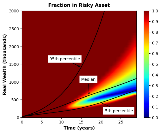
(b) $PCMo$ optimal control

Figure 8.2: Precommitment optimal control heat maps

These heat maps illustrate the optimal proportion in the risky asset as a function of current real wealth and time. The optimal proportion can be determined by comparing the color of each point to the legend on the right-hand side. Redder colors indicate a higher proportion should be invested in the risky asset, while bluer colors suggest allocating more funds to the risk-free asset.

We observe from those heatmaps in Figure 8.2 that initially the strategies recommend allocating all funds to the risky asset to maximize return. However, about 15 years later, the investment strategies begin to depend on the current wealth realized. We also note that a distinct triangular band appears in the second half of the investment horizon. This band indicates that investors should move their funds from risky to risk-free asset as their realized wealth approaches $0.6-0.8 million. Recall that the optimal threshold $W^{p\ast}$ is around $0.75 million, see Table 8.4. Financially, this threshold can be interpreted as the dollar level below which investors want to avoid falling. Therefore, if the current wealth is below this threshold, a higher allocation to risky asset is suggested to pursue the return. In contrast, if the current wealth is already at the nearby level, funds should be shifted to risk-free asset to ensure that the terminal wealth does not fall below this amount. The reason for the reallocation to risky asset in the upper right corner is that, in this area, investors have accumulated $2-3 million, which is far above the threshold level. Thus, they do not worry about falling into a poor situation and can allocate all funds to the risky asset to pursue enhanced return.

With the same optimal controls $\mathcal{U}_{0,a}^{p\ast}=\mathcal{U}_{0,o}^{p\ast}$ indicated in Figure 8.2 and the same optimal thresholds $W_{a}^{p\ast}=W_{o}^{p\ast}$ shown in Table 8.4, under the equivalence relationship presented in Lemmas 5.3 and 5.4, $PCMa$ and $PCMo$ admit the same optimal threshold/control pair $\left(W_{a}^{p\ast},\ \mathcal{U}_{0,a}^{p\ast}\right)=\left(W_{o}^{p\ast},\ \mathcal{U}_{0,o}^{p\ast}\right)$.

8.2.3 Efficient frontiers

Table 8.4 and Figure 8.2 illustrate the detailed one-to-one correspondence between $PCMa$ and $PCMo$ for a specific scalarization-optimal set. To demonstrate that this correspondence holds across the full efficient frontier, we vary the value of $\gamma$ and repeat the procedure described above. The resulting efficient frontiers are reported in Figure 8.3.

Although the two efficient frontiers shown in Figure 8.3 appear as mirror images, they plot different risk measures along the $x$-axis. In Figure 3(a), risk is quantified by $\text{CVaR}_{\alpha}(W_{T})$; increasing $\gamma_{a}$ places greater emphasis on risk reduction, resulting in strategies that increase $\text{CVaR}_{\alpha}(W_{T})$ (i.e. reduce downside risk) at the cost of lower expected terminal wealth $E[W_{T}]$. This drives the ($\text{CVaR}_{\alpha}(W_{T}),E[W_{T}])$ efficient frontier downward and to the right. In contrast, Figure 3(b) uses $\text{bPoE}_{D}(W_{T})$ as the risk measure; increasing $\gamma_{o}$ places more emphasis on lowering $\text{bPoE}_{D}(W_{T})$) at the cost of reduced $E[W_{T}]$, which drives the ($\text{bPoE}_{D}(W_{T}),E[W_{T}]$) efficient frontier downward and to the left.

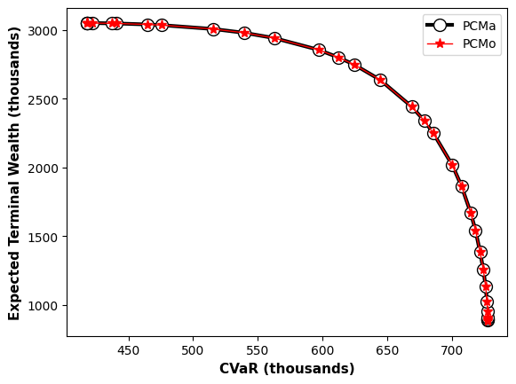
(a) Direction: $PCMa$ to $PCMo$

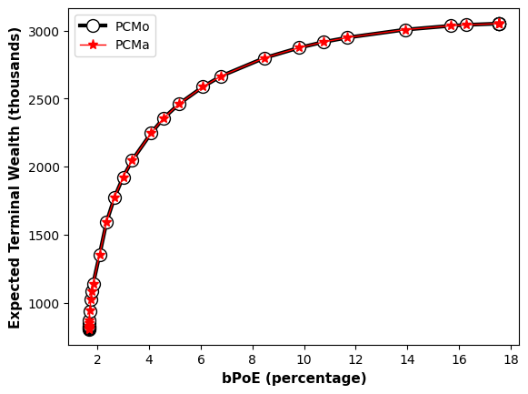
(b) Direction: $PCMo$ to $PCMa$

Figure 8.3: Equivalent efficient frontiers of $PCMa$ and $PCMo$

In Figure 3(a), each black point generated by $PCMa$ is mapped via Lemma 5.3 into a red point of $PCMa$. Conversely, Figure 3(b) starts from $PCMo$ then applies Lemma 5.4 to map to $PCMa$ points. The perfect overlap of these two frontiers in both mapping directions provides excellent numerical confirmation of the theoretical equivalence between $PCMa$ and $PCMo$ established in Lemma 5.3 and 5.4.

8.3 Time-consistent Mean–bPoE and Mean–CVaR

8.3.1 Investment outcomes

In the time-consistent setting, Remark 6.1 suggests that no global parameter mapping can preserve the same efficient frontier and optimal control/threshold structure between the TCMa and TCMb formulations. Nevertheless, we compare the investment outcomes of $TCMa$ and $TCMo$ by first matching their expected terminal wealth and then comparing other statistics, such as CVaR, bPoE, and percentiles. Specifically, for $TCMo$, we adopt the same disaster level $D$ and parameter $\gamma_{o}$ as in $PCMo$, enabling a direct comparison between $PCMo$ and $TCMo$. We then solve the $TCMo$ problem using the proposed numerical scheme to obtain its expected terminal wealth. For $TCMa$, we numerically determine the corresponding $\gamma_{a}$ using Newton’s method to match this value.

Table 8.5: Investment outcomes of $TCMa_{t_{0}}\left(\alpha,\gamma_{a}\right)$ and $TCMo_{t_{0}}\left(D,\gamma_{o}\right)$. $\alpha=0.05$, $D=668.81$, $\gamma_{a}=0.4$, $\gamma_{o}=1.6238\times 10^{4}$. Results computed using Monte Carlo simulations with $2.56\times 10^{6}$ paths. Units: thousands of dollars (real).

	$E\left[W_{T}\right]$	$\text{CVaR}_{\alpha}\left(W_{T}\right)$	$\text{bPoE}_{D}\left(W_{T}\right)$	5th $W_{T}$	50th $W_{T}$	95th $W_{T}$
$TCMa$	$2140.11$	$476.49$	$19.00\%$	$575.84$	$1618.12$	$5508.10$
$TCMo$	$2133.97$	$672.50$	$4.62\%$	$717.92$	$952.42$	$7176.15$

Table 8.5 presents the investment outcomes of $TCMa$ and $TCMo$. With the same expected terminal wealth, $TCMa$ produces a substantially lower $\text{CVaR}_{\alpha}\left(W_{T}\right)$ and a much higher $\text{bPoE}_{D}\left(W_{T}\right)$. Since a larger $\text{CVaR}_{\alpha}\left(W_{T}\right)$ and a smaller $\text{bPoE}_{D}\left(W_{T}\right)$ indicate a more favorable outcome, $TCMo$ dominates $TCMa$ in both the Mean-CVaR and Mean-bPoE sense. Thus, although the expected terminal wealth is matched, the differing risk levels imply that the scalarization optimal sets of $TCMa$ and $TCMo$ are not equivalent–as $PCMa$ and $PCMo$ are in the pre-commitment case–and no pair of efficient points coincides.

Figure 8.4: Terminal wealth distribution comparison–TCMa vs. TCMo

We note that among the other statistics reported in Table 8.5, the only metric in which $TCMa$ outperforms $TCMo$ is the median of terminal wealth. To investigate this further, we compare their terminal wealth density functions, shown in Figure 8.4. An interesting observation from this figure is that $TCMa$ concentrates more probability mass around the middle range (e.g., $0.5–2 million), whereas $TCMo$ spreads its density more into the tails.

This behavior reflects the key difference between these two risk measures. In $TCMa$, the strategy aims to minimize the average of the worst $\alpha$ fraction of outcomes at each rebalancing time, hence intuitively encouraging the portfolio to compress its distribution toward the middle to reduce extreme downside risk, which in turn elevates the median metric. By contrast, $TCMo$ enforces a fixed disaster level $D$, ensuring the wealth avoids falling below this specific wealth floor, while allowing the remainder of the distribution (including the median and upper tail) to spread more widely, if needed. Consequently, the portfolio may accept greater variance in the median or mid-range outcomes so that it can preserve or even enhance both the upside (e.g. high-end returns) and downside protection. The result is a potentially lower median outcome than Mean–CVaR, but better tail performance at the extremes (both upside and downside).

This suggests that bPoE is a strictly tail-oriented measure that prioritizes guarding against catastrophic shortfalls while still permitting meaningful upside exposure–making it especially appealing for investors focused on long-term wealth security rather than distributional tightness.

Further comparison between the $TCMo$ results in Table 8.5 and the $PCMo$ results in Table 8.4 indicates that, under the same inputs $D$ and $\gamma_{o}$, the investment outcomes of $TCMo$ closely resemble those of its precommitment counterpart. In particular, the resulting $\text{CVaR}_{\alpha}\left(W_{T}\right)$ of $TCMo$ is nearly equal to the input disaster level $D$, and its $\text{bPoE}_{D}\left(W_{T}\right)$ is close to the pre-specified confidence level $\alpha=5\%$. This consistency across the $TCMo$ and $PCMo$ formulations motivates the next investigation, which focuses on a detailed heatmap analysis of the $TCMo$ optimal rebalancing control and its comparison with that of $PCMo$.

8.3.2 Optimal rebalancing controls

Figure 8.5 displays the heat maps of the optimal controls for $TCMa$ and $TCMo$. In contrast to the precommitment case—where the optimal control heatmaps of $PCMa$ and $PCMo$ are identical—the control behaviors of $TCMa$ and $TCMo$ differ significantly.

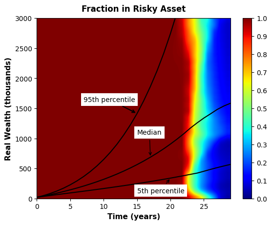
(a) $TCMa$ optimal control

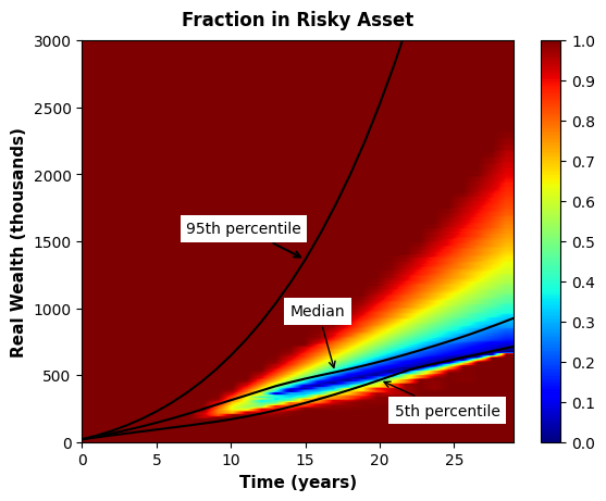
(b) $TCMo$ optimal control

Figure 8.5: Time-consistent optimal control heat maps

We highlight two key observations below.

• As shown in Figure 5(a), the $TCMa$ control depends primarily on time and exhibits a weak sensitivity to current wealth. Although our numerical experiment includes annual contributions rather than a lump-sum investment, the optimal rebalancing control remains nearly wealth-independent, consistent with the scaling property discussed earlier in Lemma 6.1 and Remark 6.1.

  Consequently, the $TCMa$ control resembles a glide-path strategy. It begins with full allocation to the risky asset to pursue growth, and gradually shifts to the risk-free asset over time to reduce risk exposure. This mirrors the principle of glide-path design: aggressive investment in early periods followed by systematic de-risking as the investment horizon shortens.

• The $TCMo$ control shown in Figure 5(b) closely resembles the $PCMo$ control in Figure 2(b). This similarity supports the idea that $TCMo$ closely mirrors $PCMo$ not only in outcomes but also in the structure of optimal rebalancing decisions. By contrast, the Mean–CVaR case shows a clear divergence between $PCMa$ and $TCMa$, with markedly different control behavior.

To better understand the structural differences between $TCMa$ and $TCMo$, we now examine the behavior of their optimal thresholds $W^{c\ast}$, which serve as the key drivers of each strategy.

8.3.3 Optimal thresholds $\bm{W^{c\ast}}$

Figure 8.6 displays heat maps of the optimal thresholds $W^{c\ast}$ for $TCMa$ and $TCMo$. In the $TCMa$ case (Figure 6(a)), $W_{a}^{c\ast}$ varies substantially, sweeping the full range from $0 to over $3.5 million as wealth increases from $0 to $3 million and time evolves.

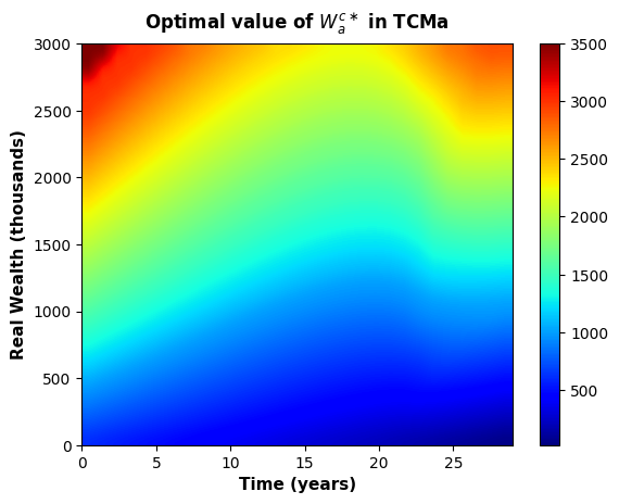
(a) $TCMa$ optimal threshold

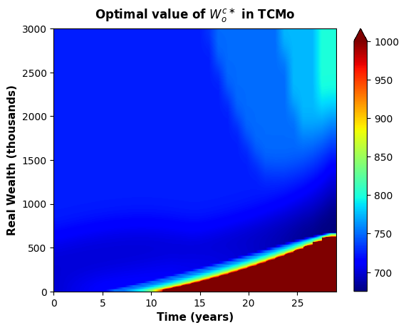
(b) $TCMo$ optimal threshold

Figure 8.6: Time-consistent optimal threshold heat maps

By contrast, in the $TCMo$ case (Figure 6(b)), more than 80% of the computed values of $W_{o}^{c\ast}$ remain within a narrow interval around the disaster level, specifically between $D\approx\$0.67$ million and $0.8 million. Interestingly, the red region in the bottom-right corner of Figure 6(b) corresponds to $W_{o}^{c\ast}=+\infty$, which arises when the current wealth is far below the disaster level $D$. In this case, the bPoE constraint $E[W_{T}]>D$ cannot be satisfied, leading to $W_{o}^{c\ast}=+\infty$ and a control of $u_{o}^{c\ast}=1$. Earlier in the investment horizon—when time to maturity is longer—the portfolio has more opportunity to satisfy the constraint, resulting in the triangular transition band observed in the lower-right portion of the heatmap.

Ignoring the singular region discussed above, we observe that $W_{o}^{c\ast}$ remains relatively stable across both time and wealth. This threshold stability implies that $TCMo$ behaves effectively like a constant-threshold policy, closely resembling its precommitment counterpart $PCMo$. The region with $W_{o}^{c\ast}=+\infty$ has little practical impact: in such low-wealth scenarios, both $PCMo$ and $TCMo$ allocate all wealth to the risky asset anyway. In contrast, the wide variation in $W_{a}^{c\ast}$ under $TCMa$ leads to rebalancing decisions that depart significantly from the constant-threshold structure of $PCMa$.

Given that $PCMo$ and $TCMo$ produce remarkably similar rebalancing controls and investment outcomes, investors may interchange the precommitment and time-consistent solutions with minimal loss of accuracy. This behavioral similarity stands in sharp contrast to the Mean–CVaR case, where time consistency leads to counterintuitive, wealth-independent controls that diverge substantially from their precommitment counterparts. The key difference lies in the structural role of the disaster level $D$: by fixing $D$ from the outset, bPoE preserves a stable tail-risk objective across time, thereby avoiding the shifting risk preferences and unintuitive rebalancing behavior commonly caused by time-consistency constraints. In this sense, bPoE not only offers intuitive tail protection but also resolves the well-known dynamic inconsistency challenges that arise in multi-period mean–risk portfolio optimization.

9 Conclusion and future work

This paper investigates the use of bPoE as a viable and intuitive alternative to CVaR in multi-period portfolio optimization for Defined Contribution plans. We formulate both pre-commitment and time-consistent Mean–bPoE and Mean–CVaR problems under realistic investment constraints and jump-diffusion dynamics, and develop a provably convergent numerical framework capable of solving all formulations.

In the pre-commitment setting, we establish a one-to-one correspondence between the scalarization optimal sets of Mean–bPoE and Mean–CVaR. Each pair of corresponding frontier points is attained by the same optimal threshold and rebalancing control, allowing bPoE to be seamlessly integrated into existing CVaR-based workflows.

In the time-consistent setting, however, this equivalence no longer holds. Mean–CVaR strategies often exhibit counterintuitive, wealth-independent controls due to dynamic threshold re-optimization. By contrast, Mean-bPoE maintains a fixed disaster level, resulting in stable shortfall thresholds and wealth-dependent rebalancing behavior that better aligns with investor preferences for a minimum acceptable terminal wealth. As a result, time-consistent Mean–bPoE closely resembles its pre-commitment counterpart—both in control structure and investment outcomes—and consistently delivers superior tail performance across a range of key metrics.

These findings show that bPoE retains the computational tractability of CVaR while offering practical advantages for long-horizon retirement planning. Its stable threshold and control structure, intuitive interpretation, and ability to resolve key limitations of time-consistent Mean–CVaR formulation make it a compelling risk measure for DC lifecycle portfolio design.

Future work may extend the bPoE framework to incorporate interim withdrawals, inflation-linked liabilities, or stochastic mortality, to assess its robustness in more realistic lifecycle settings.

Appendices

Appendix A Proof of Proposition 5.1

Consider a fixed control $\mathcal{U}_{0}\in\mathcal{A}$. Define the function

$$f(W_{o}^{p};\mathcal{U}_{0})=\mathbb{E}_{\mathcal{U}_{0}}^{X_{0}^{+},t_{0}^{+}}\left[h(W_{o}^{p};W_{T})\bigg{|}X_{0}^{-}=(s_{0},b_{0})\right],$$ (A.1)

where $h(W_{o}^{p};w)=\gamma\max\left(1-\frac{w-D}{W_{o}^{p}-D},0\right)-w$. Clearly, $h(W_{o}^{p};w)$ is continuous in $W_{o}^{p}$ for each fixed $w$. Note that $F(W_{o}^{p})=\inf_{\mathcal{U}_{0}\in\mathcal{A}}f(W_{o}^{p};\mathcal{U}_{0})$.

We now show that $f(W_{o}^{p};\mathcal{U}_{0})$ is continuous in $W_{o}^{p}$ for this fixed control $\mathcal{U}_{0}$. Specifically, for any fixed $\widehat{W}_{o}\in(D,\infty)$, and any sequence $\{W_{o}^{p\,(n)}\}$ with $W_{o}^{p\,(n)}>D$ for all $n$ and $W_{o}^{p\,(n)}\to\widehat{W}_{o}$, we will prove

$$\lim_{n\to\infty}f\bigl{(}W_{o}^{p\,(n)};\mathcal{U}_{0}\bigr{)}~=\;f\bigl{(}\widehat{W}_{o};\mathcal{U}_{0}\bigr{)}.$$ (A.2)

Equivalently, we will show

$$\lim_{n\to\infty}\mathbb{E}_{\mathcal{U}_{0}}^{X_{0}^{+},t_{0}^{+}}\Bigl{[}h\bigl{(}W_{o}^{p\,(n)};W_{T}(\omega)\bigr{)}~\big{|}~\cdot~\Bigr{]}=\mathbb{E}_{\mathcal{U}_{0}}^{X_{0}^{+},t_{0}^{+}}\Bigl{[}h\bigl{(}\widehat{W}_{o};W_{T}(\omega)\bigr{)}~\big{|}~\cdot~\Bigr{]}.$$ (A.3)

Once (A.3) is established, by the compactness of $\mathcal{A}$ and the continuity argument in parametric optimization [12], we conclude that $F(W_{o}^{p})=\inf_{\mathcal{U}_{0}\in\mathcal{A}}f(W_{o}^{p};\mathcal{U}_{0})$ is also continuous for all $W_{o}^{p}>D$.

It remains to prove (A.3), which we will do using a dominated convergence argument. In the remainder of the proofs, let $C$ and $C^{\prime}$ denote bounded constants that potentially depend only on the fixed parameters $\widehat{W}_{o}$, $\gamma$, and $D$, and are independent of $n$ and $w$. Their values may vary from line to line.

Let $\delta=\frac{1}{2}\,\bigl{(}\widehat{W}_{o}-D\bigr{)}>0$. For sufficiently large $n$, say $n\geq N_{*}$, $W_{o}^{p\,(n)}\in[\widehat{W}_{o}-\delta,\;\widehat{W}_{o}+\delta\,]~\subset~(D,\infty)$. Thus, for $n\geq N_{*}$, we have

$$W_{o}^{p\,(n)}-D~\geq~\widehat{W}_{o}-D-\delta~=~\tfrac{1}{2}\,(\widehat{W}_{o}-D).$$ (A.4)

In addition,

$$W_{o}^{p\,(n)}~\leq~\widehat{W}_{o}+\delta~=~\widehat{W}_{o}+\tfrac{1}{2}\,(\widehat{W}_{o}-D)~\leq~2\,(\widehat{W}_{o}+|D|).$$ (A.5)

Now, we bound $h(W_{o}^{p\,(n)};w)$ for sufficiently large $n$, i.e. $n\geq N_{*}$, so that $W_{o}^{p\,(n)}\in[\widehat{W}_{o}-\delta,\;\widehat{W}_{o}+\delta\,]$.

• If $w\geq W_{o}^{p\,(n)}$: we have $h(W_{o}^{p\,(n)};w)=\gamma\cdot 0-w=-w$, so $|h(W_{o}^{p\,(n)};w)|\leq|w|$.

• If $w<W_{o}^{p\,(n)}$: $\max\left(1-\tfrac{w-D}{\,W_{o}^{p\,(n)}-D},0\right)=1-\tfrac{w-D}{\,W_{o}^{p\,(n)}-D}$, so $h\bigl{(}W_{o}^{p\,(n)};w\bigr{)}~=~\gamma\,\Bigl{(}\tfrac{W_{o}^{p\,(n)}-w}{\,W_{o}^{p\,(n)}-D}\Bigr{)}\;-\;w$.

  By (A.4), for sufficiently large $n$, the denominator $(W_{o}^{p\,(n)}-D)\geq\tfrac{1}{2}\,(\widehat{W}_{o}-D)$. The numerator $(W_{o}^{p\,(n)}-w)\leq(W_{o}^{p\,(n)}+|w|)$. Thus,

  $$\Bigl{|}\gamma\,\tfrac{W_{o}^{p\,(n)}-w}{W_{o}^{p\,(n)}-D}-w\Bigr{|} \leq\gamma\,\tfrac{W_{o}^{p\,(n)}+|w|}{\tfrac{1}{2}(\widehat{W}_{o}-D)}\;+\;|w|\overset{\text{\eqref{eq:W_oD_less}}}{\leq}\tfrac{4\gamma\,\bigl{(}\widehat{W}_{o}+|D|+|w|\bigr{)}}{\widehat{W}_{o}-D}+|w|\overset{\text{(ii)}}{=}C+C^{\prime}\,|w|+|w|.$$

Hence, in either of the two cases, we can conclude that $\forall n\geq N_{*}$ and $w\geq 0$

$$\bigl{|}h\bigl{(}W_{o}^{p\,(n)};w\bigr{)}\bigr{|}~\leq~C+(C^{\prime}+1)\,\lvert w\rvert.$$

For $\omega\in\Omega$, we define $B(\omega)=C+(C^{\prime}+1)\,W_{T}(\omega)$. Hence, for $n\geq N_{*}$, $\bigl{|}h(W_{o}^{p\,(n)};W_{T}(\omega))\bigr{|}\;\leq\;B(\omega)$. By Remark 4.1, $\mathbb{E}_{\mathcal{U}_{0}}^{X_{0}^{+},t_{0}^{+}}\left[W_{T}~\big{|}~\cdot\right]<\mathcal{E}_{\max}$, so the random variable $B(\omega)$ is integrable.

By the Dominated Convergence Theorem and the pointwise continuity in $W_{o}$, we conclude that

$$\lim_{n\to\infty}\mathbb{E}_{\mathcal{U}_{0}}^{X_{0}^{+},t_{0}^{+}}\Bigl{[}h\bigl{(}W_{o}^{p\,(n)};W_{T}(\omega)\bigr{)}~\big{|}~\cdot~\Bigr{]}=\mathbb{E}_{\mathcal{U}_{0}}^{X_{0}^{+},t_{0}^{+}}\Bigl{[}\lim_{n\to\infty}h\bigl{(}W_{o}^{p\,(n)};W_{T}(\omega)\bigr{)}~\big{|}~\cdot~\Bigr{]}~=\;\mathbb{E}_{\mathcal{U}_{0}}^{X_{0}^{+},t_{0}^{+}}\Bigl{[}h\bigl{(}\widehat{W}_{o};W_{T}(\omega)\bigr{)}~\big{|}~\cdot~\Bigr{]}.$$

This is (A.3). In conclusion, for each fixed $\mathcal{U}_{0}\in\mathcal{A}$, the function $f(W_{o}^{p};\mathcal{U}_{0})$ is continuous in $W_{o}^{p}$.

Appendix B Proof of Lemma 5.1

For brevity, we will write $F(W_{o}^{p})$, with the dependence on the initial state $(s_{0},b_{0})$ understood implicitly. Let $f(W_{o}^{p};\mathcal{U}_{0})$ be as in (A.1), so $F(W_{o}^{p})=\inf_{\mathcal{U}_{0}\in\mathcal{A}}f(W_{o}^{p};\mathcal{U}_{0})$.

First, we examine the behavior of $F(W_{o}^{p})$ as $W_{o}^{p}\to D^{+}$ and $W_{o}^{p}\to\infty$. As $W_{o}^{p}\to D^{+}$, the term $\frac{1}{\,W_{o}^{p}-D\,}$ blows up, causing $F(W_{o}^{p})\to+\infty$.

For $W_{o}^{p}\rightarrow+\infty$, the term $\max\biggl{(}1-\tfrac{W_{T}-D}{\,W_{o}^{p}-D\,},\;0\biggr{)}\rightarrow 1$, and the function $F\left(W_{o}^{p}\right)$ becomes

$$\lim_{W_{o}^{p}\rightarrow+\infty}F\left(W_{o}^{p}\right) = \inf_{\mathcal{U}_{0}\in\mathcal{A}}\mathbb{E}_{\mathcal{U}_{0}}^{\,X_{0}^{+},\,t_{0}^{+}}\bigl{[}\gamma-W_{T}\bigg{|}X_{0}^{-}=(s_{0},b_{0})\bigr{]}.$$ (B.1)

The only target for optimization problem (B.1) is to maximize the expected return, so the optimal control is the strategy that fully invests in the risky asset, as noted in Remark 4.1. Denote by $\widehat{\mathcal{U}_{0}}$ the optimal control in this case. Thus, recalling $\mathcal{E}_{\max}$ from (4.3), we have

$$\lim_{W_{o}^{p}\rightarrow+\infty}F\left(W_{o}^{p}\right) = \gamma-\mathcal{E}_{\max}.$$

However, as noted in Remark 3.1, there exists a threshold value $W_{o}^{\prime}=\text{VaR}_{\mathcal{B}^{\prime}}(W_{T};\widehat{\mathcal{U}_{0}})\in(D,+\infty)$, where $\mathcal{B^{\prime}}=\mathbb{E}_{\widehat{\mathcal{U}_{0}}}^{X_{0}^{+},t_{0}^{+}}\left[\max\left(1-\frac{W_{T}-D}{W_{o}^{\prime}-D},0\right)\right]\in(0,1)$, such that

$$F\left(W_{o}^{\prime}\right)\leq f\left(W_{o}^{\prime};\widehat{\mathcal{U}_{0}}\right)=\gamma\mathcal{B}-\mathcal{E}_{\max}<\gamma-\mathcal{E}_{\max}.$$ (B.2)

Therefore, we show that $W_{o}^{p}\rightarrow+\infty$ can not be the minimizer.

By Proposition 5.1, $F(W_{o}^{p})$ is continuous on $(D,\infty)$. Combined with the boundary behavior, where $F(W_{o}^{p})\to+\infty$ as $W_{o}^{p}\to D^{+}$ and no further decrease is possible for $F(W_{o}^{p})$ as $W_{o}^{p}\to\infty$, we conclude that $\inf_{W_{o}^{p}>D}F(W_{o}^{p})$ is finite and is attained at some finite point $W_{o}^{p*}(s_{0},b_{0})\in(D,\infty)$.

Appendix C Proof of Proposition 5.2

From (5.6) and (5.3), the pre-commitment value function becomes

$$V^{p}_{o}\left(0,W_{0},t_{0}^{-}\right)=\inf_{\mathcal{U}_{0}\in\mathcal{A}}\mathbb{E}_{\mathcal{U}_{0}}^{X_{0}^{+},t_{0}^{+}}\left[\gamma\max\left(1-\frac{W_{T}-D}{W_{o}^{p*}(0,W_{0})-D},0\right)-W_{T}\bigg{|}X_{0}^{-}=(0,W_{0})\right].$$ (C.1)

Meanwhile, for $TCEQ_{t_{0}}(D,\gamma;W_{o}^{p*}(0,W_{0}))$ at $t_{0}$, the value function reads

$$\widehat{Q}^{c}_{o}(0,W_{0},t_{m})\coloneqq\inf_{\mathcal{U}_{0}}\bigg{\{}\mathbb{E}_{\mathcal{U}_{m}}^{X_{0}^{+},t_{0}^{+}}\bigg{[}\max(\widehat{W_{o}}-W_{T},\,0)-(\widehat{W_{o}}-D)\,\tfrac{W_{T}}{\gamma}\bigg{|}X_{0}^{-}=(0,W_{0})\bigg{]}\bigg{\}}.$$ (C.2)

Since $\gamma>0$, and $\widehat{W_{o}}-D>0$, any optimal control $\mathcal{U}_{0,o}^{p*}$ for (C.1) also minimizes (C.2), and vice versa. Moreover, (C.2) is solvable via standard dynamic programming over the controls. Hence, $\mathcal{U}_{0,o}^{p*}$ itself is time-consistent. This completes the proof.

Appendix D Proof of Lemma 5.2

For each fixed admissible control $\mathcal{U}_{0}\in\mathcal{A}$, we define

$$f_{a}\bigl{(}W_{a}^{p};\mathcal{U}_{0}\bigr{)}\;=\;\mathbb{E}_{\mathcal{U}_{0}}^{\,X_{0}^{+},\,t_{0}^{+}}\!\Bigl{[}\,\gamma\Bigl{(}W_{a}^{p}+\tfrac{1}{\alpha}\min(W_{T}-W_{a}^{p},\,0)\Bigr{)}+W_{T}\big{|}~\cdot~\Bigr{]}.$$

A standard dominated convergence argument (analogous to Proposition 5.1 for the pre-commitment Mean–bPoE case) shows that $f_{a}(W_{a}^{p};\mathcal{U}_{0})$ is continuous in $W_{a}^{p}$. By compactness of $\mathcal{A}$ and parametric optimization results [12], the function $F_{a}(W_{a}^{p})=\sup_{\mathcal{U}_{0}\in\mathcal{A}}f_{a}(W_{a}^{p};\,\mathcal{U}_{0})$ is continuous for all $W_{a}^{p}$ in $[0,\infty)$.

We next verify that $F_{a}(W_{a}^{p})$ cannot blow up as $W_{a}^{p}\to 0^{+}$ or $W_{a}^{p}\to\infty$. As $W_{a}^{p}\to 0^{+}$, $f_{a}$ behaves like $\mathbb{E}_{\mathcal{U}_{0}}[\gamma\,\min(W_{T},\,0)/\alpha+W_{T}|\cdot]$. Since $W_{T}$ is integrable (Remark 4.2), this expectation is finite, so no unbounded positive growth occurs.

For the case $W_{a}^{p}\to\infty$, for each fixed $W_{a}^{p}$, we partition the sample space $\Omega$ into

$$\Omega_{1}(W_{a}^{p})\;=\;\{\omega\in\Omega|\,W_{T}(\omega)\leq W_{a}^{p}\}\quad\text{and}\quad\Omega_{2}(W_{a}^{p})\;=\;\{\omega\in\Omega|\,W_{T}(\omega)>W_{a}^{p}\}.$$

On $\Omega_{1}(W_{a}^{p})$, we have $W_{T}\leq W_{a}^{p}$, so $W_{a}^{p}\;+\;\frac{1}{\alpha}\,\min(W_{T}-W_{a}^{p},\,0)~=~W_{a}^{p}\,\Bigl{(}1-\tfrac{1}{\alpha}\Bigr{)}\;+\;\tfrac{W_{T}}{\alpha}$. Since $1-\tfrac{1}{\alpha}<0$, pushing $W_{a}^{p}$ larger actually lowers this part.

On $\Omega_{2}(W_{a}^{p})$, $W_{T}>W_{a}^{p}$, so $\min(W_{T}-W_{a}^{p},0)=0$. Therefore,

$$f_{a}\bigl{(}W_{a}^{p};\mathcal{U}_{0}\bigr{)} =\mathbb{E}_{\mathcal{U}_{0}}^{\,X_{0}^{+},\,t_{0}^{+}}\left[\,\gamma\,W_{a}^{p}\;+\;W_{T}\right|~\cdot~]=\int_{\{W_{T}(\omega)>W_{a}^{p}\}}\bigl{[}\gamma\,W_{a}^{p}+W_{T}(\omega)\bigr{]}\,d\mathbb{P}(\omega)$$

$$=\gamma\,W_{a}^{p}\,\mathbb{P}\!\bigl{(}W_{T}>W_{a}^{p}\bigr{)}+\int_{\{W_{T}(\omega)>W_{a}^{p}\}}\!\!W_{T}(\omega)\,d\mathbb{P}(\omega).$$

$$\overset{(i)}{\leq}\gamma\,W_{a}^{p}\frac{\mathbb{E}_{\mathcal{U}_{0}}^{\,X_{0}^{+},\,t_{0}^{+}}[\,W_{T}\,]}{\,W_{a}^{p}\,}+\mathbb{E}_{\mathcal{U}_{0}}^{\,X_{0}^{+},\,t_{0}^{+}}\big{[}\,W_{T}\mathbb{I}_{\{W_{T}>W_{a}^{p}\}}\big{]}$$

$$\overset{(ii)}{=}\gamma\mathbb{E}_{\mathcal{U}_{0}}^{\,X_{0}^{+},\,t_{0}^{+}}[\,W_{T}\,]+\int_{W_{a}^{p}}^{\infty}\mathbb{P}(W_{T}>u)du+W_{a}^{p}\mathbb{P}(W_{T}>W_{a}^{p}).$$

Here, (i) follows from Markov’s inequality, while (ii) is due to Fubini’s theorem. Since $W_{T}$ has finite expectation, standard tail‐integration arguments imply that, as $W_{a}^{p}\to\infty$, both $\int_{W_{a}^{p}}^{\infty}\mathbb{P}(W_{T}>u)du$ and and $W_{a}^{p}\mathbb{P}(W_{T}>W_{a}^{p})$ vanish. Therefore, in all cases, no blow-up can occur as $W_{a}^{p}\to\infty$.

In summary, $F_{a}(W_{a}^{p})$ remains finite and is continuous on $[0,\infty)$, and it does not blow up at either $0$ or $+\infty$. Therefore, $\sup_{W_{a}^{p}\geq 0}F_{a}(W_{a}^{p})$ must be attained at some finite $W_{a}^{p*}\in[0,\infty)$. This completes the proof.

Appendix E Proof of Lemma 5.3

By Lemma 4.2, the scalarization optimal set $\mathcal{S}_{a}(\alpha,\gamma_{a})$ for the Mean–CVaR problem is nonempty. As such, the existence of a point $\bigl{(}\mathcal{C}_{a}^{*},\,\mathcal{E}_{a}^{*}\bigr{)}\in\mathcal{S}_{a}(\alpha,\gamma_{a})$ is guaranteed. Furthermore, the associated optimal threshold $W_{a}^{p*}$ exists by Lemma 5.2. Therefore, $\gamma_{o}$ given by (5.10) is well-defined.

Let $\mathcal{U}_{0,a}^{p\ast}$ denote the optimal control associated with $\bigl{(}\mathcal{C}_{a}^{*},\,\mathcal{E}_{a}^{*}\bigr{)}$. Then using definitions in (4.7), the point $\bigl{(}\mathcal{C}_{a}^{*},\,\mathcal{E}_{a}^{*}\bigr{)}$ can be expressed in terms of $W_{a}^{p*}$ and $\mathcal{U}_{0,a}^{p\ast}$ as follows:

$$\mathcal{C}_{a}^{*}=W_{a}^{p\ast}+\tfrac{1}{\alpha}\mathbb{E}_{\mathcal{U}_{0,a}^{p\ast}}\left[\min\left(W_{T}-W_{a}^{p\ast},0\right)\right],\quad\text{and}\quad\mathcal{E}_{a}^{*}=\mathbb{E}_{\mathcal{U}_{0,a}^{p\ast}}\left[W_{T}\right].$$ (E.1)

In order to prove that $\bigl{(}\mathcal{B}_{o}^{*},\,\mathcal{E}_{o}^{*}\bigr{)}=\bigl{(}\alpha,\,\mathcal{E}_{a}^{*}\bigr{)}$ is in $\mathcal{S}_{o}\!\bigl{(}\mathcal{C}_{a}^{*},\gamma_{o}\bigr{)}$, by definition of the Mean–bPoE scalarization optimal set given in (4.5), we need to show

$$\gamma_{o}\alpha-\mathcal{E}_{a}^{*}=\underset{\begin{subarray}{c}W_{o}^{p}>\mathcal{C}_{a}^{*},\\ \mathcal{U}_{0}\end{subarray}}{\inf}\left\{\tfrac{\gamma_{a}(W_{a}^{p*}-\mathcal{C}_{a}^{*})}{\alpha}\mathbb{E}_{\mathcal{U}_{0}}\left[\max\left(1-\tfrac{W_{T}-\mathcal{C}_{a}^{*}}{W_{o}^{p}-\mathcal{C}_{a}^{*}},\,0\right)\right]-\mathbb{E}_{\mathcal{U}_{0}}[W_{T}]\right\}.$$ (E.2)

We first carry out further manipulations on both sides of (E.2). Using (5.10) and the formula for $\mathcal{C}_{a}^{*}$ in (E.1) on the lhs of (E.2), we obtain

lhs of (E.2) $$= \gamma_{a}(\,W_{a}^{p*}\;-\;\mathcal{C}_{a}^{*}\,)-\mathcal{E}_{a}^{*}$$ (E.3)

$$= -\tfrac{\gamma_{a}}{\alpha}\mathbb{E}_{\mathcal{U}_{0,a}^{p\ast}}\left[\min\left(W_{T}-W_{a}^{p\ast},0\right)\right]-\mathcal{E}_{a}^{*}.$$

Simplifying the $\max(\cdot,0)$ term on the rhs of (E.2), noting $W_{o}^{p}-\mathcal{C}_{a}^{*}>0$, gives

rhs of (E.2) $$=\underset{\begin{subarray}{c}W_{o}^{p}>\mathcal{C}_{a}^{*},\\ \mathcal{U}_{0}\end{subarray}}{\inf}\left\{-\tfrac{\gamma_{a}(W_{a}^{p*}-\mathcal{C}_{a}^{*})}{\alpha\left(W_{o}^{p}-\mathcal{C}_{a}^{*}\right)}\mathbb{E}_{\mathcal{U}_{0}}\left[\min\left(W_{T}-W_{o}^{p},0\right)\right]-\mathbb{E}_{\mathcal{U}_{0}}\left[W_{T}\right]\right\}.$$ (E.4)

$$\overset{(i)}{=}\!-\!\underset{\begin{subarray}{c}W_{o}^{p}>\mathcal{C}_{a}^{*},\\ \mathcal{U}_{0}\end{subarray}}{\sup}\!\!\left\{\tfrac{\gamma_{a}(W_{a}^{p*}-\mathcal{C}_{a}^{*})}{\alpha\left(W_{o}^{p}-\mathcal{C}_{a}^{*}\right)}\,\mathbb{E}_{\mathcal{U}_{0}}\left[\min\left(W_{T}-W_{o}^{p},0\right)\right]+\mathbb{E}_{\mathcal{U}_{0}}\left[W_{T}\right]\right\}.$$ (E.5)

Here, (i) is due to the identity $-\underset{z\in\mathcal{X}}{\sup}\{f(z)\}=\underset{z\in\mathcal{X}}{\inf}\{-f(z)\}$ for any function $f$ and any set $\mathcal{X}$.

By noting that, with $W_{o}^{p}=W_{a}^{p\ast}$ and $\mathcal{U}_{0}=\mathcal{U}_{0,a}^{p\ast}$ in (E.4), we obtain (E.3) as a candidate for the infimum in (E.4). This leads to the following inequality

$$\underset{\begin{subarray}{c}W_{o}^{p}>\mathcal{C}_{a}^{*},\\ \mathcal{U}_{0}\end{subarray}}{\inf}\left\{\tfrac{-\gamma_{a}(W_{a}^{p*}-\mathcal{C}_{a}^{*})}{\alpha\left(W_{o}^{p}-\mathcal{C}_{a}^{*}\right)}\mathbb{E}_{\mathcal{U}_{0}}\left[\min\left(W_{T}-W_{o}^{p},0\right)\right]-\mathbb{E}_{\mathcal{U}_{0}}\left[W_{T}\right]\right\}\leq-\tfrac{\gamma_{a}}{\alpha}\mathbb{E}_{\mathcal{U}_{0,a}^{p\ast}}\left[\min\left(W_{T}-W_{a}^{p\ast},0\right)\right]\,-\,\mathcal{E}_{a}^{*}.$$

This shows that the rhs of (E.2) is less than or equal to its lhs.

To show the reverse inequality, note that the right-hand side of (E.2) equals the right-hand side of (E.5). Therefore, noting $\gamma_{a}W_{a}^{p*}$ is a constant, it suffices to show

$$\text{rhs of \eqref{eq: opt Mean_bPOE v3*}}\;\geq\;\text{lhs of \eqref{eq:scar_*}},~~\text{or equivalently},~~-\,\text{(rhs of \eqref{eq: opt Mean_bPOE v3*})}+\gamma_{a}W_{a}^{p*}\;\leq\;-\,\text{(lhs of \eqref{eq:scar_*})}+\gamma_{a}W_{a}^{p*}.$$

That is, with the lhs of (E.2) given in (E.3), we will show

$$\underset{\begin{subarray}{c}W_{o}^{p}>\mathcal{C}_{a}^{*},\\ \mathcal{U}_{0}\end{subarray}}{\sup}\left\{\gamma_{a}W_{a}^{p*}+\tfrac{\gamma_{a}(W_{a}^{p*}-\mathcal{C}_{a}^{*})}{\alpha\left(W_{o}^{p}-\mathcal{C}_{a}^{*}\right)}\,\mathbb{E}_{\mathcal{U}_{0}}\left[\min\left(W_{T}-W_{o}^{p},0\right)\right]+\mathbb{E}_{\mathcal{U}_{0}}\left[W_{T}\right]\right\}$$ (E.6)

$$\qquad\qquad\qquad\qquad\leq\gamma_{a}W_{a}^{p*}+\tfrac{\gamma_{a}}{\alpha}\mathbb{E}_{\mathcal{U}_{0,a}^{p\ast}}\left[\min\left(W_{T}-W_{a}^{p\ast},0\right)\right]+\mathcal{E}_{a}^{*}.$$

Starting from the lhs of (LABEL:eq:equ), we have

lhs of (LABEL:eq:equ) $$\overset{(i)}{\leq}\underset{\begin{subarray}{c}W_{o}^{p},\,\mathcal{U}_{0}\end{subarray}}{\sup}\left\{\gamma_{a}W_{o}^{p}+\tfrac{\gamma_{a}(W_{o}^{p}-\mathcal{C}_{a}^{*})}{\alpha\left(W_{o}^{p}-\mathcal{C}_{a}^{*}\right)}\,\mathbb{E}_{\mathcal{U}_{0}}\left[\min\left(W_{T}-W_{o}^{p},0\right)\right]+\mathbb{E}_{\mathcal{U}_{0}}\left[W_{T}\right]\right\}$$

$$\overset{(ii)}{=}\underset{\begin{subarray}{c}W_{o}^{p},\,\mathcal{U}_{0}\end{subarray}}{\sup}\left\{\gamma_{a}W_{o}^{p}+\tfrac{\gamma_{a}}{\alpha}\,\mathbb{E}_{\mathcal{U}_{0}}\left[\min\left(W_{T}-W_{o}^{p},0\right)\right]+\mathbb{E}_{\mathcal{U}_{0}}\left[W_{T}\right]\right\}$$

$$\overset{(iii)}{=}\gamma_{a}W_{a}^{p*}+\tfrac{\gamma_{a}}{\alpha}\mathbb{E}_{\mathcal{U}_{0,a}^{p\ast}}\left[\min\left(W_{T}-W_{a}^{p\ast},0\right)\right]\,+\,\mathcal{E}_{a}^{*},$$

which is the inequality (LABEL:eq:equ) we need to prove. Here, in (i), the inequality arises because $W_{a}^{p\ast}$ is replaced by a free variable $W_{o}^{p}$, and the supremum is taken over a larger set for $W_{o}^{p}$; (ii) follows from simplification; and (iii) is due to the fact that $W_{o}^{p}$ is a dummy variable for the optimization, noting $\mathcal{U}_{0,a}^{p\ast}$ and $W_{a}^{p*}$ are the optimal control/threshold pair associated with $\bigl{(}\mathcal{C}_{a}^{*},\mathcal{E}_{a}^{*}\bigr{)}$. This concludes the proof.

Appendix F Proof of Lemma 5.4

By Lemma 4.1, the existence of a point $\bigl{(}\mathcal{B}_{o}^{*},\,\mathcal{E}_{o}^{*}\bigr{)}\in\mathcal{S}_{o}\!\bigl{(}D,\gamma_{o}\bigr{)}$ is guaranteed. Furthermore, the associated optimal threshold $W_{o}^{p*}>D$ exists by Lemma 5.1. Therefore, $\gamma_{a}$ given by (5.11) is well-defined.

Let $\mathcal{U}_{0,o}^{p\ast}$ denote the optimal control associated with $\bigl{(}\mathcal{B}_{o}^{*},\,\mathcal{E}_{o}^{*}\bigr{)}$. Then using definitions in (4.1), the point $\bigl{(}\mathcal{B}_{o}^{*},\,\mathcal{E}_{o}^{*}\bigr{)}$ can be expressed in terms of $W_{o}^{p*}$ and $\mathcal{U}_{0,o}^{p\ast}$ as follows:

$$\mathcal{B}_{o}^{*}=\mathbb{E}_{\mathcal{U}_{0,o}^{p\ast}}\left[\max\left(1-\tfrac{W_{T}-D}{W_{o}^{p\ast}-D},\,0\right)\right]=-\tfrac{\mathbb{E}_{\mathcal{U}_{0,o}^{p\ast}}\left[\min\left(W_{T}-W_{o}^{p\ast},\,0\right)\right]}{W_{o}^{p\ast}-D},\quad\text{and}\quad\mathcal{E}_{o}^{*}=\mathbb{E}_{\mathcal{U}_{0,o}^{p\ast}}\left[W_{T}\right].$$ (F.1)

From (F.1), we can express the disaster level $D$ in terms of $W_{o}^{p\ast}$, $\mathcal{B}_{o}^{*}$, and the expectation as

$$D=W_{o}^{p\ast}+\tfrac{1}{\mathcal{B}_{o}^{*}}\,\mathbb{E}_{\mathcal{U}_{0,o}^{p\ast}}\left[\min\left(W_{T}-W_{o}^{p\ast},\,0\right)\right].$$ (F.2)

In order to prove that $\bigl{(}\mathcal{C}_{a}^{*},\mathcal{E}_{a}^{*}\bigr{)}=\bigl{(}D,\,\mathcal{E}_{o}^{*}\bigr{)}$ belongs to $\mathcal{S}_{a}\!\bigl{(}\mathcal{B}_{o}^{*},\gamma_{a}\bigr{)}$, by definition (4.10), we need to verify

$$\gamma_{a}D+\mathcal{E}_{o}^{\ast} = \underset{W_{a}^{p},\ \mathcal{U}_{0}}{\sup}\left\{\gamma_{a}W_{a}^{p}+\frac{\gamma_{a}}{\mathcal{B}_{o}^{\ast}}\mathbb{E}_{\mathcal{U}_{0}}\left[\min{\left(W_{T}-W_{a}^{p},0\right)}\right]+\mathbb{E}_{\mathcal{U}_{0}}\left[W_{T}\right]\right\}.$$ (F.3)

The lhs of (F.3) can be written as

$$\gamma_{a}D+\mathcal{E}_{o}^{\ast} = \gamma_{a}W_{o}^{p\ast}+\frac{\gamma_{a}}{\mathcal{B}_{o}^{\ast}}\mathbb{E}_{\mathcal{U}_{0,o}^{p\ast}}\left[\min{\left(W_{T}-W_{o}^{p\ast},0\right)}\right]+\mathcal{E}_{o}^{\ast}.$$ (F.4)

By noting that with $W_{a}^{p}=W_{o}^{p\ast}$ and $\mathcal{U}_{0}=\mathcal{U}_{0,o}^{p\ast}$, we obtain a candidate for the supremum of rhs of (F.3). This shows that

$$\gamma_{a}D+\mathcal{E}_{o}^{\ast} \leq \underset{W_{a}^{p},\ \mathcal{U}_{0}}{\sup}\left\{\gamma_{a}W_{a}^{p}+\frac{\gamma_{a}}{\mathcal{B}_{o}^{\ast}}\mathbb{E}_{\mathcal{U}_{0}}\left[\min{\left(W_{T}-W_{a}^{p},0\right)}\right]+\mathbb{E}_{\mathcal{U}_{0}}\left[W_{T}\right]\right\}.$$ (F.5)

To establish the reverse inequality, we note that the rhs of (F.3) can be written as

$$\underset{W_{a}^{p},\ \mathcal{U}_{0}}{\sup}\left\{\gamma_{a}W_{a}^{p}+\frac{\gamma_{a}}{\mathcal{B}_{o}^{\ast}}\mathbb{E}_{\mathcal{U}_{0}}\left[\min{\left(W_{T}-W_{a}^{p},0\right)}\right]+\mathbb{E}_{\mathcal{U}_{0}}\left[W_{T}\right]\right\}$$ (F.6)

$$= \underset{W_{a}^{p},\ \mathcal{U}_{0}}{\sup}\left\{\frac{\gamma_{o}\mathcal{B}_{o}^{\ast}W_{a}^{p}}{W_{o}^{p\ast}-D}+\frac{\gamma_{o}}{W_{o}^{p\ast}-D}\mathbb{E}_{\mathcal{U}_{0}}\left[\min{\left(W_{T}-W_{a}^{p},0\right)}\right]+\mathbb{E}_{\mathcal{U}_{0}}\left[W_{T}\right]\right\}\quad\left(\gamma_{a}=\frac{\gamma_{o}\mathcal{B}_{o}^{\ast}}{W_{o}^{p\ast}-D}\right)$$

$$= \underset{W_{a}^{p},\ \mathcal{U}_{0}}{\sup}\left\{\frac{\gamma_{o}\mathcal{B}_{o}^{\ast}W_{a}^{p}}{W_{o}^{p\ast}-D}-\gamma_{o}\mathbb{E}_{\mathcal{U}_{0}}\left[\max{\left(\frac{W_{a}^{p}-D}{W_{o}^{p\ast}-D}-\frac{W_{T}-D}{W_{o}^{p\ast}-D},0\right)}\right]+\mathbb{E}_{\mathcal{U}_{0}}\left[W_{T}\right]\right\}$$

$$= -\underset{W_{a}^{p},\ \mathcal{U}_{0}}{\inf}\left\{-\frac{\gamma_{o}\mathcal{B}_{o}^{\ast}W_{a}^{p}}{W_{o}^{p\ast}-D}+\gamma_{o}\mathbb{E}_{\mathcal{U}_{0}}\left[\max{\left(\frac{W_{a}^{p}-D}{W_{o}^{p\ast}-D}-\frac{W_{T}-D}{W_{o}^{p\ast}-D},0\right)}\right]-\mathbb{E}_{\mathcal{U}_{0}}\left[W_{T}\right]\right\}.$$

And lhs of (F.3) can be written as

$$\gamma_{a}D+\mathcal{E}_{o}^{\ast} = \frac{\gamma_{o}\mathcal{B}_{o}^{\ast}D}{W_{o}^{p\ast}-D}+\mathcal{E}_{o}^{\ast}$$ (F.7)

So our goal is to show

$$\gamma_{a}D+\mathcal{E}_{o}^{\ast} \geq \underset{W_{a}^{p},\ \mathcal{U}_{0}}{\sup}\left\{\gamma_{a}W_{a}^{p}+\frac{\gamma_{a}}{\mathcal{B}_{o}^{\ast}}\mathbb{E}_{\mathcal{U}_{0}}\left[\min{\left(W_{T}-W_{a}^{p},0\right)}\right]+\mathbb{E}_{\mathcal{U}_{0}}\left[W_{T}\right]\right\}$$

$$\frac{\gamma_{o}\mathcal{B}_{o}^{\ast}D}{W_{o}^{p\ast}-D}+\mathcal{E}_{o}^{\ast} \geq -\underset{W_{a}^{p},\ \mathcal{U}_{0}}{\inf}\left\{-\frac{\gamma_{o}\mathcal{B}_{o}^{\ast}W_{a}^{p}}{W_{o}^{p\ast}-D}+\gamma_{o}\mathbb{E}_{\mathcal{U}_{0}}\left[\max{\left(\frac{W_{a}^{p}-D}{W_{o}^{p\ast}-D}-\frac{W_{T}-D}{W_{o}^{p\ast}-D},0\right)}\right]-\mathbb{E}_{\mathcal{U}_{0}}\left[W_{T}\right]\right\}$$

$$-\frac{\gamma_{o}\mathcal{B}_{o}^{\ast}D}{W_{o}^{p\ast}-D}-\mathcal{E}_{o}^{\ast} \leq \underset{W_{a}^{p},\ \mathcal{U}_{0}}{\inf}\left\{-\frac{\gamma_{o}\mathcal{B}_{o}^{\ast}W_{a}^{p}}{W_{o}^{p\ast}-D}+\gamma_{o}\mathbb{E}_{\mathcal{U}_{0}}\left[\max{\left(\frac{W_{a}^{p}-D}{W_{o}^{p\ast}-D}-\frac{W_{T}-D}{W_{o}^{p\ast}-D},0\right)}\right]-\mathbb{E}_{\mathcal{U}_{0}}\left[W_{T}\right]\right\}$$

$$\frac{\gamma_{o}\mathcal{B}_{o}^{\ast}\left(W_{o}^{p\ast}-D\right)}{W_{o}^{p\ast}-D}-\mathcal{E}_{o}^{\ast} \leq \underset{W_{a}^{p},\ \mathcal{U}_{0}}{\inf}\left\{\frac{\gamma_{o}\mathcal{B}_{o}^{\ast}\left(W_{o}^{p\ast}-W_{a}^{p}\right)}{W_{o}^{p\ast}-D}+\gamma_{o}\mathbb{E}_{\mathcal{U}_{0}}\left[\max{\left(\frac{W_{a}^{p}-D}{W_{o}^{p\ast}-D}-\frac{W_{T}-D}{W_{o}^{p\ast}-D},0\right)}\right]-\mathbb{E}_{\mathcal{U}_{0}}\left[W_{T}\right]\right\}$$

$$\gamma_{o}\mathcal{B}_{o}^{\ast}-\mathcal{E}_{o}^{\ast} \leq \underset{W_{a}^{p},\ \mathcal{U}_{0}}{\inf}\left\{\frac{\gamma_{o}\mathcal{B}_{o}^{\ast}\left(W_{o}^{p\ast}-W_{a}^{p}\right)}{W_{o}^{p\ast}-D}+\gamma_{o}\mathbb{E}_{\mathcal{U}_{0}}\left[\max{\left(\frac{W_{a}^{p}-D}{W_{o}^{p\ast}-D}-\frac{W_{T}-D}{W_{o}^{p\ast}-D},0\right)}\right]-\mathbb{E}_{\mathcal{U}_{0}}\left[W_{T}\right]\right\}$$ (F.8)

Now we focus on rhs of (F.8),

$$\underset{W_{a}^{p},\ \mathcal{U}_{0}}{\inf}\left\{\frac{\gamma_{o}\mathcal{B}_{o}^{\ast}\left({\color[rgb]{0,0,0}W_{o}^{p\ast}}-W_{a}^{p}\right)}{W_{o}^{p\ast}-D}+\gamma_{o}\mathbb{E}_{\mathcal{U}_{0}}\left[\max{\left(\frac{W_{a}^{p}-D}{{\color[rgb]{0,0,0}W_{o}^{p\ast}}-D}-\frac{W_{T}-D}{{\color[rgb]{0,0,0}W_{o}^{p\ast}}-D},0\right)}\right]-\mathbb{E}_{\mathcal{U}_{0}}\left[W_{T}\right]\right\}$$

$$\overset{(i)}{\geq} \underset{W_{a}^{p},\ \mathcal{U}_{0}}{\inf}\left\{\frac{\gamma_{o}\mathcal{B}_{o}^{\ast}\left({\color[rgb]{0,0,0}W_{a}^{p}}-W_{a}^{p}\right)}{W_{o}^{p\ast}-D}+\gamma_{o}\mathbb{E}_{\mathcal{U}_{0}}\left[\max{\left(\frac{W_{a}^{p}-D}{{\color[rgb]{0,0,0}W_{a}^{p}}-D}-\frac{W_{T}-D}{{\color[rgb]{0,0,0}W_{o}^{p\ast}}-D},0\right)}\right]-\mathbb{E}_{\mathcal{U}_{0}}\left[W_{T}\right]\right\}$$

$$= \underset{\mathcal{U}_{0}}{\inf}\left\{\gamma_{o}\mathbb{E}_{\mathcal{U}_{0}}\left[\max{\left(1-\frac{W_{T}-D}{{\color[rgb]{0,0,0}W_{o}^{p\ast}}-D},0\right)}\right]-\mathbb{E}_{\mathcal{U}_{0}}\left[W_{T}\right]\right\}$$

$$\overset{(ii)}{\geq} \underset{W_{o}^{p}>D,\ \mathcal{U}_{0}}{\inf}\left\{\gamma_{o}\mathbb{E}_{\mathcal{U}_{0}}\left[\max{\left(1-\frac{W_{T}-D}{{\color[rgb]{0,0,0}W_{o}^{p}}-D},0\right)}\right]-\mathbb{E}_{\mathcal{U}_{0}}\left[W_{T}\right]\right\}$$

$$\overset{(iii)}{=} \gamma_{o}\mathcal{B}_{o}^{\ast}-\mathcal{E}_{o}^{\ast}.$$

Here, (i) arises because $W_{o}^{p\ast}$ is replaced by a free variable $W_{a}^{p}$; (ii) results from replacing $W_{o}^{p\ast}$ by a free variable $W_{o}^{p}>D$. Recall $W_{o}^{p\ast}>D$, so a free variable $W_{o}^{p}>D$ indeed provides a larger range; (iii) is due to the fact that $W_{o}^{p\ast}$ and $\mathcal{U}_{0,o}^{\ast}$ are the optimal solution associated with $\left(\mathcal{B}_{o}^{\ast},\mathcal{E}_{o}^{\ast}\right)$. This concludes the proof.

Appendix G An infinite series representation of $\bm{g(y,\Delta t)}$

Under the log-transformation, the jump-diffusion dynamics in (2.8)—where $\log(\xi)$ follows an asymmetric double-exponential distribution with density given in (2.7)—admit an infinite series representation for the conditional transition density $g(y,\Delta t)$ [60][Corollary 3.1], as presented below. Define

$$\alpha=\frac{\sigma^{2}}{2}\,\Delta t,\quad\beta=\left(\mu-\lambda\kappa-\frac{\sigma^{2}}{2}\right)\Delta t,\quad\theta=-\lambda\Delta t.$$

Then

$$g(y,\Delta t)=g_{0}(y,\Delta t)+\sum_{\ell=1}^{\infty}\Delta g_{\ell}(y,\Delta t),$$ (G.1)

where $g_{0}(y,\Delta t)=\frac{\exp\left(\theta-\frac{(\beta+y)^{2}}{4\alpha}\right)}{\sqrt{4\pi\alpha}}$, and the remaining terms $\Delta g_{\ell}(y,\Delta t)$ are given by:

$$g_{\ell}(y,\Delta t)= \frac{e^{\theta}}{\sqrt{4\pi\alpha}}\frac{\left(\lambda\Delta t\right)^{\ell}}{\ell!}\left[\sum_{k=1}^{\ell}\,Q_{1}^{\ell,k}\,\left(\eta_{1}\,\sqrt{2\alpha}\right)^{k}\,\mathrm{e}^{\eta_{1}\,\left({{\beta+y}}\right)+\eta_{1}^{2}\alpha}\,\mathrm{Hh}_{k-1}\left(\eta_{1}\sqrt{2\alpha}+\frac{{{\beta+y}}}{\sqrt{2\alpha}}\right)\right.$$

$$\qquad\qquad\qquad\left.+\sum_{k=1}^{\ell}\,Q_{2}^{\ell,k}\,\left(\eta_{2}\,\sqrt{2\alpha}\right)^{k}\,\mathrm{e}^{-\eta_{2}\,\left({{\beta+y}}\right)+\eta_{2}^{2}\alpha}\,\mathrm{Hh}_{k-1}\left(\eta_{2}\sqrt{2\alpha}-\frac{{{\beta+y}}}{\sqrt{2\alpha}}\right)\right],$$ (G.2)

where $Q_{1}^{\ell,k}$, $Q_{2}^{\ell,k}$ and $\mathrm{Hh}_{k}$ are defined as follows

$$Q_{1}^{\ell,k} =\sum_{i=k}^{\ell-1}\binom{\ell-k-1}{i-k}\binom{\ell}{i}\left(\frac{\eta_{1}}{\eta_{1}+\eta_{2}}\right)^{i-k}\left(\frac{\eta_{2}}{\eta_{1}+\eta_{2}}\right)^{\ell-i}p_{up}^{i}(1-p_{up})^{\ell-i},\quad 1\leq k\leq\ell-1,$$

$$Q_{2}^{\ell,k} =\sum_{i=k}^{\ell-1}\binom{\ell-k-1}{i-k}\binom{\ell}{i}\left(\frac{\eta_{1}}{\eta_{1}+\eta_{2}}\right)^{\ell-i}\left(\frac{\eta_{2}}{\eta_{1}+\eta_{2}}\right)^{i-k}p_{up}^{\ell-i}(1-p_{up})^{i},\quad 1\leq k\leq\ell-1,$$ (G.3)

where $Q_{1}^{\ell,\ell}=p_{up}^{\ell}$ and $Q_{2}^{\ell,\ell}=(1-p_{up})^{\ell}$, and

$$Hh_{k}(x)=\frac{1}{k!}\int_{x}^{\infty}\left(z-x\right)^{k}e^{-\frac{1}{2}z^{2}}dz,\text{ with }Hh_{-1}(x)=e^{-x^{2}/2},\text{ and }Hh_{0}(x)=\sqrt{2\pi}\text{NorCDF}(-x).$$ (G.4)

Here, NorCDF denotes CDF of standard normal distribution $\mathcal{N}(0,1)$. For this case, we note that function $Hh_{\ell}(\cdot)$ can be evaluated very efficiently using the standard normal density function and standard normal distribution function via the three-term recursion [1]

$$k\,Hh_{k}(x)=Hh_{k-2}(x)-xHh_{k-1}(x),\quad k\geq 1.$$

For computational purposes, the infinite series in (G.1) is truncated after $N_{g}$ terms, yielding the approximation $g(y,\Delta t;N_{g})$. As $N_{g}\to\infty$, the approximation becomes exact. For finite $N_{g}$, however, truncation introduces an error. As shown in [60], this truncation error can be bounded by

$$\left|g(y,\Delta t)-g(y,\Delta t;N_{g})\right|\leq\frac{\left(\lambda\Delta t\right)^{N_{g}+1}}{(N_{g}+1)!}\,\frac{1}{\sqrt{2\pi\sigma^{2}\Delta t}}.$$ (G.5)

Therefore, from (G.5), as $N_{g}\to\infty$, we have $\frac{\left(\lambda\Delta t\right)^{N_{g}+1}}{(N_{g}+1)!}\rightarrow 0$, and the truncated approximation $g(y,\Delta t;N_{g})$ converges to the exact density $g(y,\Delta t)$. For a given tolerance $\epsilon_{g}>0$, one can choose $N_{g}$ such that the truncation error satisfies $\left|g(y,\Delta t)-g(y,\Delta t;N_{g})\right|<\epsilon_{g}$. This can be ensured by requiring $N_{g}$ to satisfy $\displaystyle\frac{\left(\lambda\Delta t\right)^{N_{g}+1}}{(N_{g}+1)!}\leq\epsilon_{g}\sqrt{2\pi\sigma^{2}\Delta t}$. It then follows that if $\epsilon_{g}=\mathcal{O}(h)$, we can choose $N_{g}=\mathcal{O}(\ln(h^{-1}))$ as $h\to 0$.

Appendix H Proof of Theorem 7.1

We now present the convergence proof for the pre-commitment Mean–bPoE/CVaR formulations.

H.1 Value function convergence

We first establish the convergence of the value function: $\displaystyle\lim_{h\to 0}\bigl{|}V_{h}^{p}(s_{0},b_{0},t_{0}^{-})-V^{p}(s_{0},b_{0},t_{0}^{-})\bigr{|}=0$. The proof consists of two parts: we first establish a convergence bound for the inner optimisation problem at a fixed discrete threshold, and then analyse the convergence of the outer optimisation at time $t_{0}$ as $h\to 0$.

H.1.1 Inner optimization

For now, we fix $W^{p}\in\Gamma$ and consider the inner control problem, which corresponds to a portfolio optimization over the bounded domain $\Omega\times\mathcal{T}\cup\{T\}$. We show that the scheme for this inner problem satisfies three key properties: $\ell_{\infty}$-stability, monotonicity, and local consistency. To facilitate the analysis, we reformulate both the pre-commitment Mean–bPoE/CVaR problem in Definition 7.1 and the numerical scheme (7.15)–(7.21), including both interior and boundary equations, each in a unified operator form.

For notational convenience, let $\hat{x}=(y,b,W^{p})\in\Omega\times\Gamma$ and $\hat{x}^{m}=(\hat{x},t_{m})$ with $t_{m}\in\mathcal{T}\cup\{t_{M}=T\}$. For fixed $W^{p}\in\Gamma$, we denote by $\widehat{V}^{p}(W^{p},t_{m+1})$ the function $\widehat{V}^{p}(y,b,W^{p},t_{m+1})$. When clear from context, we write $\widehat{V}^{p}(y,b,\cdot,t_{m+1})$ or $\widehat{V}^{p}(\cdot,t_{m+1})$ in place of the full expression.

Given a state $(y,b)$ and rebalancing control $u_{m}\in\mathcal{Z}$, we recall the definitions $y^{+}=y^{+}(y,b,u_{m})$ and $b^{+}=b^{+}(y,b,u_{m})$ from (7.2). Including both interior and boundary equations, we now express the pre-commitment Mean–bPoE/CVaR problem at the reference point $\hat{x}^{m}$ (with fixed $W^{p}$) using the operator $\mathcal{D}(\cdot)$ as follows:

$$\widehat{V}^{p}\big{(}\hat{x}^{m}\big{)}=\mathcal{D}\left(\hat{x}^{m},\,\widehat{V}^{p}(\cdot,t_{m+1}^{-})\right) =\begin{cases}\underset{u_{m}\in\mathcal{Z}}{\inf}\,\widehat{V}\left(y^{+}(y,b,u_{m}),b^{+}(y,b,u_{m}),\cdot,t_{m}^{+}\right),&\text{Mean--bPoE},\\ \underset{u_{m}\in\mathcal{Z}}{\sup}\,\widehat{V}\left(y^{+}(y,b,u_{m}),b^{+}(y,b,u_{m}),\cdot,t_{m}^{+}\right),&\text{Mean--CVaR}.\end{cases}$$ (H.1)

In both cases, the quantity $\widehat{V}\in\{\widehat{V}_{o}^{p},\,\widehat{V}_{a}^{p}\}$ denotes the appropriate value function, and is given as follows: $\widehat{V}\left(y^{+}(y,b,u_{m}),b^{+}(y,b,u_{m}),\cdot,t_{m}^{+}\right)=\ldots$

$$\widehat{V}\left(y^{+}(y,be^{r\Delta t},u_{m}),b^{+}(y,be^{r\Delta t},u_{m}),\cdot,t_{m+1}^{-}\right) \quad\quad(y,b)\in\Omega_{y_{\min}},$$ (H.2a)

$$\int_{y_{\min}^{\dagger}}^{y_{\max}^{\dagger}}\widehat{V}\left(y^{+}(y^{\prime},be^{r\Delta t},u_{m}),b^{+}(y,be^{r\Delta t},u_{m}),\cdot,t_{m+1}^{-}\right)\,g(y-y^{\prime},\Delta t)~dy^{\prime} \quad\quad(y,b)\in\Omega_{\scalebox{0.7}{\text{in}}},$$ (H.2b)

$$e^{\mu\Delta t}~\widehat{V}\left(y^{+}(y,be^{r\Delta t},u_{m}),b^{+}(y,be^{r\Delta t},u_{m}),\cdot,t_{m+1}^{-}\right) \quad\quad(y,b)\in\Omega_{y_{\max}}.$$ (H.2c)

Let $\Omega^{h}\times\Gamma^{h}$ denote the computational grid parameterized by $h$. Let $\Omega_{\scalebox{0.7}{\text{in}}}^{h}$ denote the interior sub-grid, and $\Omega_{y_{\min}}^{h}$, $\Omega_{y_{\max}}^{h}$ the boundary sub-grids in $y$. Including both interior and boundary equations, we now write the numerical scheme at the reference node $\hat{x}_{n,j}^{k,m}=(y_{n},b_{j},W_{k},t_{m})\in\Omega^{h}\times\Gamma^{h}\times\{t_{m}\}$ in operator form via $\mathcal{D}_{h}(\cdot)$ as follows:

$$\widehat{V}_{h}^{p}\big{(}\hat{x}_{n,j}^{k,m}\big{)} =\mathcal{D}_{h}\left(\hat{x}_{n,j}^{k,m},\,\left\{\widehat{V}_{h}^{p}\big{(}\hat{x}_{l,j}^{k,(m+1)-}\big{)}\right\}_{l=-N^{\dagger}/2}^{N^{\dagger}/2}\right)$$

$$=\begin{cases}\underset{\{u_{i}\}}{\min}\,\widehat{V}_{h}\left(y^{+}(y_{n},b_{j},u_{i}),b^{+}(y_{n},b_{j},u_{i}),\cdot,t_{m}^{+}\right),&\text{Mean--bPoE},\\ \underset{\{u_{i}\}}{\max}\,\widehat{V}_{h}\left(y^{+}(y_{n},b_{j},u_{i}),b^{+}(y_{n},b_{j},u_{i}),\cdot,t_{m}^{+}\right),&\text{Mean--CVaR}.\end{cases}$$ (H.3)

In both cases, the quantity $\widehat{V}_{h}\in\{\widehat{V}_{o,h}^{p},\,\widehat{V}_{a,h}^{p}\}$ denotes the appropriate discrete approximation, and is defined as $\widehat{V}_{h}\left(y^{+}(y_{n},b_{j},u_{i}),b^{+}(y_{n},b_{j},u_{i}),\cdot,t_{m}^{+}\right)=\ldots$

$$\widehat{V}_{h}\left(y^{+}(y_{n},b_{j}e^{r\Delta t},u_{i}),b^{+}(y_{n},b_{j}e^{r\Delta t},u_{i}),\cdot,t_{m+1}^{-}\right) \quad(y_{n},b_{j})\in\Omega_{y_{\min}}^{h},$$ (H.4a)

$$\sum_{l=-N^{\dagger}/2}^{N^{\dagger}/2}\varphi_{l}~g(y_{n}-y_{l},\Delta t)\widehat{V}_{h}\left(y^{+}(y_{l},b_{j}e^{r\Delta t},u_{i}),b^{+}(y_{n},b_{j}e^{r\Delta t},u_{i}),\cdot,t_{m+1}^{-}\right) \quad(y_{n},b_{j})\in\Omega_{\scalebox{0.7}{\text{in}}}^{h},$$ (H.4b)

$$e^{\mu\Delta t}\widehat{V}_{h}\left(y^{+}(y_{n},b_{j}e^{r\Delta t},u_{i}),b^{+}(y_{n},b_{j}e^{r\Delta t},u_{i}),\cdot,t_{m+1}^{-}\right) \quad(y_{n},b_{j})\in\Omega_{y_{\max}}^{h},$$ (H.4c)

where $y^{+}(y^{\prime},b^{\prime},u_{m})$ and $b^{+}=b^{+}(y^{\prime},b^{\prime},u_{m})$ are given by (7.2).

Let $\epsilon_{g}$ denote the truncation error bound in approximating the transition density function $g(\cdot,\Delta t)$ by its $N_{g}$-term series expansion; that is, $|g(\cdot,\Delta t)-g(\cdot,\Delta t;N_{g})|<\epsilon_{g}$. Suppose linear interpolation is used for the intervention step. Also suppose that as $h\to 0$, $N_{y}^{\dagger},N_{b},N_{w},N_{u},N_{g},\to\infty$. Following the general framework of convergence proofs for numerical approximations of solutions in the stochastic control setting (see [32, 5]), we show that our scheme, for each fixed $W_{k}\in\Gamma^{h}$, is $\ell_{\infty}$-stable, locally consistent, and monotone. Specifically,

• $\ell_{\infty}$-stability: the scheme (7.15)–(7.21) for $V_{h}^{p}(\cdot)$ satisfies the bound:

  $$\sup_{h>0}\big{\|}\widehat{V}_{h}^{p}(W_{k},t_{m})\big{\|}_{\infty}<\infty,\quad\forall t_{m}\in\mathcal{T}\cup\{T\},\text{ as $h\to 0$}.$$ (H.5)

  Here, we have $\big{\|}\widehat{V}_{h}^{p}(W_{k},t_{m})\big{\|}_{\infty}=\max_{n,j}|\widehat{V}_{h}^{p}\big{(}\hat{x}_{n,j}^{k,m}\big{)}|$, where $(y_{n},b_{j},W_{k})\in\Omega^{h}\times\Gamma^{h}$ and $W_{k}$ is fixed.

• Local consistency: For any smooth test function $\phi\in\mathcal{C}^{\infty}(\Omega\cup\Omega_{b_{\max}}\times[0,T])$ for a sufficiently small $h,\chi$,

  $$\mathcal{D}_{h}\left(\hat{x}_{n,j}^{k,m},\left\{\widehat{V}_{h}^{p}\big{(}\hat{x}_{l,j}^{k,(m+1)-}\big{)}+\chi\right\}_{l=-N^{\dagger}/2}^{N^{\dagger}/2}\right)=\mathcal{D}\left(\hat{x}_{n,j}^{k,m},\widehat{V}^{p}(\cdot,t_{m+1}^{-})\right)+\mathcal{E}\left(\hat{x}_{n,j}^{k,m},\epsilon_{g},h\right)+\mathcal{O}\left(\chi+h\right),$$ (H.6)

  where $\mathcal{E}(\hat{x}_{n,j}^{k,m},\epsilon_{g},h)\to 0$ as $\epsilon_{g},h\to 0$.

• Monotonicity: the numerical scheme $\mathcal{D}_{h}(\cdot)$ satisfies

  $$\mathcal{D}_{h}\left(\hat{x}_{n,j}^{k,m},\left\{\varphi_{l,j}^{k,{m+1}}\right\}_{l=-N^{\dagger}/2}^{N^{\dagger}/2}\right)\leq\mathcal{D}_{h}\left(\hat{x}_{n,j}^{k,m},\left\{\psi_{l,j}^{k,m+1})\right\}_{l=-N^{\dagger}/2}^{N^{\dagger}/2}\right)$$ (H.7)

  for bounded discrete data sets $\left\{\varphi_{l,j}^{k,{m+1}}\right\}$ and $\left\{\psi_{l,j}^{k,m+1}\right\}$ having $\left\{\varphi_{l,j}^{k,{m+1}}\right\}\leq\left\{\psi_{l,j}^{k,m+1}\right\}$, where the inequality is understood in the component-wise sense.

The $\ell_{\infty}$-stability follows from a maximum-principle argument, which applies since $\Omega$ is bounded, together with the monotonicity of linear interpolation, which is preserved under the scheme’s $\min/\max$ operations. Monotonicity of the scheme itself follows from this same interpolation structure. Local consistency is established via standard interpolation error analysis, Taylor expansion of the smooth test function, truncation error from the infinite series, and compactness of the admissible control set $\mathcal{Z}$. For further details, we refer the reader to [60], which develops similar techniques in the context of pre-commitment Mean–Variance optimization.

Convergence bound for the inner problem: We now state a convergence bound for the inner problem using $h$-indexed notation to reflect the role of mesh refinement. A generic grid point in $\Omega_{\scalebox{0.7}{\text{in}}}^{h}$ is denoted by $(y_{h},b_{h})$, and we write $W_{h}\in\Gamma^{h}$ to emphasize the $h$-dependence of the discretized threshold. The following bound holds for the inner optimization problem at fixed $W_{h}\in\Gamma^{h}$:

Let $(y^{\prime},b^{\prime})\in\Omega$ be arbitrary. Suppose that linear interpolation is used for intervention step. Under the assumption that $\epsilon_{g}\to 0$ as $h\to 0$, we have: for each $m\in\{M-1,\ldots,0\}$ and any sequence $\{(y_{h},b_{h})\}$ with $(y_{h},b_{h})\in\Omega_{\scalebox{0.7}{\text{in}}}^{h}$ and $(y_{h},b_{h})\to(y^{\prime},b^{\prime})$ as $h\to 0$,

$$\bigl{|}\widehat{V}_{h}^{p}(y_{h},b_{h},W_{h},t_{m})-\widehat{V}^{p}(y^{\prime},b^{\prime},W_{h},t_{m})\bigr{|}\leq\chi_{h}^{m},\quad\chi_{h}^{m}\text{ is bounded }\forall h>0\text{ and }\chi_{h}^{m}\to 0\text{ as }h\to 0.$$ (H.8)

The result in (H.8) can be proved using $\ell_{\infty}$-stability (H.5), local consistency (H.6), monotonicity (I.5), and backward induction on $m$.

H.1.2 Outer optimization at time $\bm{t_{0}}$

At time $t_{0}$, for each fixed $W^{p}\in\Gamma$ (resp. $W_{h}\in\Gamma^{h}$), we define

$$F(W^{p})\quad\big{(}\text{resp.\ }F_{h}(W_{h})\big{)}:=\begin{cases}~~\widehat{V}_{o}^{p}(y_{0},b_{0},W_{o}^{p},t_{0})\quad\big{(}\text{resp.\ }~~~\widehat{V}_{o,h}^{p}(y_{0},b_{0},W_{h},t_{0})\big{)}&\text{Mean--bPoE},\\ -\widehat{V}_{a}^{p}(y_{0},b_{0},W^{p}_{a},t_{0})\quad\big{(}\text{resp.\ }-\widehat{V}_{a,h}^{p}(y_{0},b_{0},W_{h},t_{0})\big{)}&\text{Mean--CVaR}.\end{cases}$$ (H.9)

We include the minus sign in the Mean–CVaR case to unify both problems under a minimization framework for the outer optimization. We note that the function $F$ is continuous in $W^{p}$. Moreover, since the problem is localized, $F(W^{p})$ remains finite on $\Gamma$. For any $W^{p}\in\Gamma$, the triangle inequality yields:

$$\bigl{|}F_{h}(W_{h})-F(W^{p})\bigr{|}\leq\bigl{|}F_{h}(W_{h})-F(W_{h})\bigr{|}+\bigl{|}F(W_{h})-F(W^{p})\bigr{|}\overset{\text{(i)}}{\leq}\chi_{h}+\bigl{|}F(W_{h})-F(W^{p})\bigr{|}\overset{\text{(ii)}}{\xrightarrow[h\to 0]{}}0.$$ (H.10)

Here, (i) follows from the definitions of $F$ and $F_{h}$, and from the bound (H.8) applied at $t_{0}$, which gives $\bigl{|}F_{h}(W_{h})-F(W_{h})\bigr{|}\leq\chi_{h}$, where $\chi_{h}\to 0$ as $h\to 0$. The limit in (ii) is due to the denseness of $\Gamma^{h}$ in $\Gamma$ as $h\to 0$: for any $W^{p}\in\Gamma$, there exists a sequence $\{W_{h}\}$ with $W_{h}\in\Gamma^{h}$ and $W_{h}\to W^{p}$ as $h\to 0$, and since $F$ is continuous, it follows that $\lim_{h\to 0}F(W_{h})=F(W^{p})$.

We now show

$$\lim_{h\to 0}~\min_{W_{h}\in\Gamma_{h}}F_{h}(W_{h})=\min_{W^{p}\in\Gamma}F(W^{p})$$ (H.11)

by establishing the corresponding upper and lower bounds:

$$\limsup_{\,h\to 0}\min_{W_{h}\in\Gamma^{h}}F_{h}(W_{h})\leq\min_{W^{p}\in\Gamma}F(W^{p}),\quad\text{and}\quad\liminf_{\,h\to 0}\min_{W_{h}\in\Gamma^{h}}F_{h}(W_{h})\geq\min_{W^{p}\in\Gamma}F(W^{p}).$$ (H.12)

Once (H.11) is established, the convergence of the value function follows:

$$\lim_{h\to 0}\bigl{\lvert}V_{h}^{p}(s_{0},b_{0},t_{0}^{-})-V^{p}(s_{0},b_{0},t_{0}^{-})\bigr{\rvert}=0.$$

We first show the $\limsup$ portion of (H.12). Pick an arbitrary $\varepsilon>0$ and let $\rho=\min_{W\in\Gamma}F(W)$. By definition of $\min$, there exists $W^{\prime}\in\Gamma$ with $F(W^{\prime})\leq\rho+\tfrac{\varepsilon}{2}$. Next, because $\Gamma^{h}\to\Gamma$ as $h\to 0$, choose $W_{h}\in\Gamma^{h}$ so $\lvert W_{h}-W^{\prime}\rvert\to 0$. By continuity, $F(W_{h})\leq F(W^{\prime})+\tfrac{\varepsilon}{2}$. Recalling the inner problem convergence bound (H.8), we have $\lvert F_{h}(W_{h})-F(W_{h})\rvert\leq\chi_{h}$, where $\chi_{h}\to 0$ as $h\to 0$. Then

$$\min_{W_{i}\in\Gamma^{h}}F_{h}(W_{i})\leq F_{h}(W_{h})\leq F(W_{h})+\chi_{h}\leq F(W^{\prime})+\tfrac{\varepsilon}{2}+\chi_{h}\leq\rho+\varepsilon+\chi_{h}.$$

For sufficiently small $h$, $\chi_{h}\leq\varepsilon$. Thus $\min_{W_{i}\in\Gamma^{h}}F_{h}(W_{i})\leq\rho+2\varepsilon$. Hence, we obtain the $\limsup$ portion

$$\limsup_{h\to 0}\min_{W_{i}\in\Gamma^{h}}F_{h}(W_{i})\leq\min_{W\in\Gamma}F(W).$$

For the $\liminf$ portion of (H.12), we fix any $W_{h}\in\Gamma^{h}$. By the inner problem convergence bound (H.8), we have $F_{h}(W_{h})\geq F(W_{h})-\chi_{h}$, and since $\min_{W\in\Gamma}F(W)\leq F(W_{h})$, we have $F_{h}(W_{h})\geq\min_{W\in\Gamma}F(W)-\chi_{h}$, from which, taking the minimum over $W_{h}$ gives $\min_{W_{h}\in\Gamma^{h}}\,F_{h}(W_{k})\geq\min_{W\in\Gamma}F(W)-\chi_{h}$. Taking limit both sides of the above $h\to 0$, noting $\chi_{h}\to 0$, gives the $\liminf$ portion:

$$\liminf_{\,h\to 0}\min_{W_{h}\in\Gamma^{h}}F_{h}(W_{h})\geq\min_{W\in\Gamma}F(W).$$

H.2 Convergence to optimal threshold $\bm{W^{p\ast}}$

We denote by $W_{h}^{\ast}$ the computed optimal threshold which minimizes the discrete objective $F_{h}(\cdot)$ defined in (H.9), i.e. $F_{h}\bigl{(}W_{h}^{\ast}\bigr{)}=\min_{\,W_{h}\in\Gamma^{h}}\,F_{h}(W_{h})$. For a fixed $h>0$, as noted earlier, the value $W_{h}^{\ast}$ is obtained by exhaustive search over the discrete set $\Gamma^{h}$, ensuring that the discrete global minimiser is found. Since $\Gamma$ is compact, and the discrete thresholds $W_{h}^{\ast}\in\Gamma^{h}\subset\Gamma$ all lie in this compact set, any infinite sequence $\{W_{h}^{\ast}\}$ has a subsequence $\{W_{h_{k}}^{\ast}\}$ convergent to some $W^{\ast}\in\Gamma$, i.e. $W_{h_{k}}^{\ast}\;\xrightarrow[k\to\infty]{}W^{\ast}\in\Gamma$.

We now show that $W^{\ast}$ is indeed the optimal threshold of the pre-commitment Mean-bPoE/CVaR problem:

$$W^{\ast}\in\mathop{\rm arg\,min}_{W\in\Gamma}F(W),\quad\text{$F(\cdot)$ defined in \eqref{eq:FFh}}.$$

Because $\Gamma^{h}\subset\Gamma$ and by the convergence bound for the inner problem in (H.8), for any fixed $W\in\Gamma^{h}$, we have $\bigl{|}F_{h}(W)-F(W)\bigr{|}\to 0$ as $h\to 0$. This implies $\bigl{|}F_{h}(W_{h_{k}}^{\ast})-F(W_{h_{k}}^{\ast})\bigr{|}\;\xrightarrow[k\to\infty]{}0$. Since $W_{h_{k}}^{\ast}\to W^{\ast}$ and $F$ is continuous, we get $F(W_{h_{k}}^{\ast})\to F(W^{\ast})$. Thus, we also have $F_{h}(W_{h_{k}}^{\ast})\to F(W^{\ast})$ as $k\to\infty$. Putting together, we arrive at

$$F_{h}\bigl{(}W_{h_{k}}^{\ast}\bigr{)}\;\xrightarrow[k\to\infty]{}F\bigl{(}W^{\ast}\bigr{)}.$$ (H.13)

By convergence of the outer optimization problem at time $t_{0}$ given in (H.11):

$$\min_{W_{h}\in\Gamma^{h}}F_{h}(W_{h})\;\xrightarrow[h\to 0]{}\min_{W^{p}\in\Gamma}F(W^{p}).$$ (H.14)

From (H.14), we conclude that

$$F_{h}\bigl{(}W_{h_{k}}^{\ast}\bigr{)}=\min_{\,W\in\Gamma^{h_{k}}}F_{h_{k}}(W)\;\;\xrightarrow[k\to\infty]{}\min_{\,W^{p}\in\Gamma}F(W^{p}),$$

which, together with (H.13), gives $F(W^{\ast})=\min_{\,W^{p}\in\Gamma}F(W^{p})$, meaning $W^{\ast}\in\mathop{\rm arg\,min}_{\,W\in\Gamma}F(W)$, as wanted. This concludes the proof.

Appendix I Proof of Theorem 7.2

For the purpose of analysis, the time-consistent Mean–bPoE/CVaR formulations and their numerical schemes can be expressed using unified operators similar to $\mathcal{D}$ and $\mathcal{D}_{h}$ defined in (H.1)–(H.1.1) for the pre-commitment case. Specifically, including both interior and boundary equations, we write the time-consistent Mean–bPoE/CVaR problem at the reference point $\hat{x}^{m}=(y,b,W^{c},t_{m})$ using the operator $\mathcal{G}(\cdot)$ as follows:
$\widehat{V}^{c}\big{(}\hat{x}^{m}\big{)}=\mathcal{G}\left(\hat{x}^{m},\,\widehat{V}^{c}(\cdot,t_{m+1}^{-})\right)=\ldots$

$$\ldots=\begin{cases}\underset{W^{c}_{o}\in\Gamma_{o}}{\inf}\,\widehat{U}_{o}^{c}\left(y,b,W_{o}^{c},t_{m}^{+}\right)&\text{Mean--bPoE},\\ \quad\text{ where }\widehat{U}_{o}^{c}\left(y,b,W_{o}^{c},t_{m}^{+}\right)=\underset{u_{m}\in\mathcal{Z}}{\inf}\,\widehat{V}_{o}^{c}\left(y^{+}(y,b,u_{m}),b^{+}(y,b,u_{m}),W_{o}^{c},t_{m}^{+}\right),\\ \underset{W^{c}_{a}\in\Gamma_{a}}{\sup}\,\widehat{U}_{a}^{c}\left(y,b,W_{a}^{c},t_{m}^{+}\right)&\text{Mean--CVaR}.\\ \quad\text{ where }\widehat{U}_{a}^{c}\left(y,b,W_{a}^{c},t_{m}^{+}\right)=\underset{u_{m}\in\mathcal{Z}}{\sup}\,\widehat{V}_{a}^{c}\left(y^{+}(y,b,u_{m}),b^{+}(y,b,u_{m}),W_{a}^{c},t_{m}^{+}\right),\end{cases}$$ (I.1)

Here, in both case, the quantity $\widehat{V}\in\{\widehat{V}_{o}^{c},\,\widehat{V}_{a}^{c}\}$ denotes the appropriate value function, and is defined in (H.2), with $y^{+}(y^{\prime},b^{\prime},u_{m})$ and $b^{+}=b^{+}(y^{\prime},b^{\prime},u_{m})$ given by (7.2).

The numerical scheme at the reference node $\hat{x}_{n,j}^{k,m}=(y_{n},b_{j},W_{k},t_{m})\in\Omega^{h}\times\Gamma^{h}\times\{t_{m}\}$, including both interior and boundary cases, can be written in unified operator form via $\mathcal{G}_{h}(\cdot)$ as follows:

$$\widehat{V}_{h}^{v}\big{(}\hat{x}_{n,j}^{k,m}\big{)}=\mathcal{G}_{h}\left(\hat{x}_{n,j}^{k,m},\,\left\{\widehat{V}_{h}^{c}\big{(}\hat{x}_{l,j}^{k,(m+1)-}\big{)}\right\}_{l=-N^{\dagger}/2}^{N^{\dagger}/2}\right)$$

$$=\begin{cases}\underset{\{W_{\iota}\}}{\min}\,\widehat{U}_{h}^{c}(y_{n},b_{j},W_{\iota},t_{m}^{+})&\text{Mean--bPoE},\\ \text{ where }\widehat{U}_{h}^{c}(y_{n},b_{j},W_{\iota},t_{m}^{+})=\underset{\{u_{i}\}}{\min}\,\widehat{V}_{o,h}^{c}\left(y^{+}(y_{n},b_{j},u_{i}),b^{+}(y_{n},b_{j},u_{i}),W_{\iota},t_{m}^{+}\right),\\ \underset{\{W_{\iota}\}}{\max}\,\widehat{U}_{h}^{c}(y_{n},b_{j},W_{\iota},t_{m}^{+})&\text{Mean--CVaR}.\\ \text{ where }\widehat{U}_{h}^{c}(y_{n},b_{j},W_{\iota},t_{m}^{+})=\underset{\{u_{i}\}}{\max}\,\widehat{V}_{a,h}^{c}\left(y^{+}(y_{n},b_{j},u_{i}),b^{+}(y_{n},b_{j},u_{i}),W_{\iota},t_{m}^{+}\right),\end{cases}$$ (I.2)

In both cases, the quantity $\widehat{V}_{h}\in\{\widehat{V}_{o,h}^{c},\,\widehat{V}_{a,h}^{c}\}$ denotes the appropriate discrete approximation, and is defined in (H.4), with $y^{+}(y^{\prime},b^{\prime},u_{i})$ and $b^{+}=b^{+}(y^{\prime},b^{\prime},u_{i})$ given by (7.2).

We then establish $\ell_{\infty}$-stability, consistency, and monotonicity of our scheme. Specifically,

• $\ell_{\infty}$-stability: the scheme (7.29)–(7.33) for $V_{h}^{c}(\cdot)$ satisfies the bound:

  $$\sup_{h>0}\big{\|}\widehat{V}_{h}^{c}(W_{k},t_{m})\big{\|}_{\infty}<\infty,\quad\forall t_{m}\in\mathcal{T}\cup\{T\},\text{ as $h\to 0$}.$$ (I.3)

• Local consistency: For any smooth test function $\phi\in\mathcal{C}^{\infty}(\Omega\cup\Omega_{b_{\max}}\times[0,T])$ for a sufficiently small $h,\chi$,

  $$\mathcal{G}_{h}\left(\hat{x}_{n,j}^{k,m},\left\{\widehat{V}_{h}^{c}\big{(}\hat{x}_{l,j}^{k,(m+1)-}\big{)}+\chi\right\}_{l=-N^{\dagger}/2}^{N^{\dagger}/2}\right)=\mathcal{G}\left(\hat{x}_{n,j}^{k,m},\widehat{V}^{c}(\cdot,t_{m+1}^{-})\right)+\mathcal{E}^{\prime}\left(\hat{x}_{n,j}^{k,m},\epsilon_{g},h\right)+\mathcal{O}\left(\chi+h\right),$$ (I.4)

  where $\mathcal{E}^{\prime}(\hat{x}_{n,j}^{k,m},\epsilon_{g},h)\to 0$ as $\epsilon_{g},h\to 0$.

• Monotonicity: the numerical scheme $\mathcal{G}_{h}(\cdot)$ satisfies

  $$\mathcal{G}_{h}\left(\hat{x}_{n,j}^{k,m},\left\{\varphi_{l,j}^{k,{m+1}}\right\}_{l=-N^{\dagger}/2}^{N^{\dagger}/2}\right)\leq\mathcal{G}_{h}\left(\hat{x}_{n,j}^{k,m},\left\{\psi_{l,j}^{k,m+1})\right\}_{l=-N^{\dagger}/2}^{N^{\dagger}/2}\right)$$ (I.5)

  for bounded discrete data sets $\left\{\varphi_{l,j}^{k,{m+1}}\right\}$ and $\left\{\psi_{l,j}^{k,m+1}\right\}$ having $\left\{\varphi_{l,j}^{k,{m+1}}\right\}\leq\left\{\psi_{l,j}^{k,m+1}\right\}$, where the inequality is understood in the component-wise sense.

Proofs of these properties follow the same steps as in the pre-commitment case (see Appendix H for details), as the re-optimization of thresholds at each state–time node introduces no additional difficulty. This is because the $\min/\max$ operation over thresholds is simply a monotone transformation of real values.

By $\ell_{\infty}$-stability, local consistency, and monotonicity, we obtain a convergence bound analogous to the pre-commitment case:

Let $(y^{\prime},b^{\prime})\in\Omega$ be arbitrary. Suppose that linear interpolation is used for intervention step. Under the assumption that $\epsilon_{g}\to 0$ as $h\to 0$, we have: for a fixed discretized threshold value $W_{h}\in\Gamma^{h}$, and each $m\in\{M-1,\ldots,0\}$ and any sequence $\{(y_{h},b_{h})\}$ with $(y_{h},b_{h})\in\Omega_{\scalebox{0.7}{\text{in}}}^{h}$ and $(y_{h},b_{h})\to(y^{\prime},b^{\prime})$ as $h\to 0$,

$$\bigl{|}\widehat{V}_{h}^{c}(y_{h},b_{h},W_{h},t_{m})-\widehat{V}^{c}(y^{\prime},b^{\prime},W_{h},t_{m})\bigr{|}\leq\chi_{h}^{m},\quad\chi_{h}^{m}\text{ is bounded }\forall h>0\text{ and }\chi_{h}^{m}\to 0\text{ as }h\to 0.$$ (I.6)

Value function convergence.

To handle the threshold re-optimization (unifying both Mean-bPoE and Mean-CVaR problems), we follow the same approach as in the pre-commitment case (Section H.1.2) but do it locally at each node: fix $(y^{\prime},b^{\prime},t_{m})\in\Omega_{\scalebox{0.7}{\text{in}}}\times\{t_{m}\}$ (resp. $(y_{h},b_{h},t_{m})\in\Omega_{\scalebox{0.7}{\text{in}}}^{h}\times\{t_{m}\}$) and let the threshold $W^{c}\in\Gamma$ (resp. $W_{h}\in\Gamma^{h}$) we define $F(y^{\prime},b^{\prime},W^{c},t_{m})$ (resp. $F_{h}(y_{h},b_{h},W_{h},t_{m})$) as follows

$$F(\cdot)\quad\big{(}\text{resp.\ }F_{h}(\cdot)\big{)}:=\begin{cases}~~\widehat{U}_{o}^{c}(y^{\prime},b^{\prime},W_{o}^{c},t_{m})\quad\big{(}\text{resp.\ }~~~\widehat{U}_{o,h}^{c}(y_{h},b_{h},W_{h},t_{m})\big{)}&\text{Mean--bPoE},\\ -\widehat{U}_{a}^{c}(y^{\prime},b^{\prime},W^{c}_{a},t_{m})\quad\big{(}\text{resp.\ }-\widehat{U}_{a,h}^{c}(y_{h},b_{h},W_{h},t_{m})\big{)}&\text{Mean--CVaR}.\end{cases}$$ (I.7)

Here, the functions $\widehat{U}_{o}^{c}(\cdot)$/$\widehat{U}_{a}^{c}(\cdot)$ and $\widehat{U}_{o,h}^{c}(\cdot)$/$\widehat{U}_{a,h}^{c}(\cdot)$ are defined in (7.26) and (7.32), respectively. In the CVaR case, the (-) sign ensures we do a minimization rather than a maximization, so that we can unify both problems under a minimization framework for the re-optimization of the threshold. We note that

$$\widehat{V}^{c}(y^{\prime},b^{\prime},t_{m})\;:=\;\min_{\,W^{c}\in\Gamma}\,F\bigl{(}y^{\prime},b^{\prime},W^{c},t_{m}\bigr{)},\quad\text{and}\quad\widehat{V}_{h}^{c}(y_{h},b_{h},t_{m})\;:=\;\min_{\,W_{h}\in\Gamma^{h}}\,F_{h}\bigl{(}y_{h},b_{h},W_{h},t_{m}\bigr{)}.$$ (I.8)

We now establish

$$\lim_{h\to 0}\Bigl{\lvert}\min_{W_{h}\in\Gamma^{h}}F_{h}(y_{h},b_{h},W_{h},t_{m})\;-\;\min_{W^{c}\in\Gamma}F(y^{\prime},b^{\prime},W^{c},t_{m})\Bigr{\rvert}=0\quad\text{as }(y_{h},b_{h})\to(y^{\prime},b^{\prime})$$ (I.9)

using the $\limsup$ and $\liminf$ arguments: $(y_{h},b_{h})\to(y^{\prime},b^{\prime})$ as $h\to 0$, we have

$$\limsup_{h\to 0}\min_{W_{h}\in\Gamma^{h}}F_{h}(y_{h},b_{h},W_{h},t_{m}) \leq\min_{W^{c}\in\Gamma}F(y^{\prime},b^{\prime},W^{c},t_{m}),$$ (I.10)

$$\liminf_{h\to 0}\min_{W_{h}\in\Gamma^{h}}F_{h}(y_{h},b_{h},W_{h},t_{m}) \geq\min_{W^{c}\in\Gamma}F(y^{\prime},b^{\prime},W^{c},t_{m}).$$

Once (I.9) is established, recalling (I.8), we conclude that

$$\lim_{h\to 0}\,\Bigl{\lvert}\widehat{V}_{h}^{c}(y_{h},b_{h},t_{m})\;-\;\widehat{V}^{c}(y^{\prime},b^{\prime},t_{m})\Bigr{\rvert}\;=\;0\quad\text{as }(y_{h},b_{h})\to(y^{\prime},b^{\prime}).$$

By exponentiating $s=e^{y}$ and letting $(s_{h},b_{h})\to(s^{\prime},b^{\prime})$, we recover the value function convergence in the original coordinates stated in (7.34).

We first show the $\limsup$ portion of (I.10). This is similar to the proof for the pre-commitment case. By the definition of the continuous minimum,

$$\exists W^{\ast}\in\Gamma\text{ such that }F\bigl{(}y^{\prime},b^{\prime},W^{\ast},t_{m}\bigr{)}\leq\min_{W^{c}\in\Gamma}F(y^{\prime},b^{\prime},W^{c},t_{m})+\tfrac{\varepsilon}{2}.$$ (I.11)

Because $\Gamma^{h}\subset\Gamma$ is dense as $h\to 0$, choose $W_{h}\in\Gamma^{h}$ such that $\lvert W_{h}-W^{\ast}\rvert\to 0$. By a triangle inequality and for sufficiently small $h$, we have

$$\bigl{|}F_{h}(y_{h},b_{h},W_{h},t_{m})-F(y^{\prime},b^{\prime},W^{\ast},t_{m})\bigr{|} \leq\bigl{|}F_{h}(y_{h},b_{h},W_{h},t_{m})-F(y^{\prime},b^{\prime},W_{h},t_{m})\bigr{|}$$

$$\quad+\bigl{|}F(y^{\prime},b^{\prime},W_{h},t_{m})-F(y^{\prime},b^{\prime},W^{\ast},t_{m})\bigr{|}\overset{(i)}{\leq}\tfrac{\varepsilon}{4}+\tfrac{\varepsilon}{4}=\tfrac{\varepsilon}{2}$$

Here, in (i), by (I.6), for sufficiently small $h$, we can bound the first term by $\tfrac{\varepsilon}{4}$, while due to the continuity of $F(\cdot)$ in the threshold argument, the second term can be bounded above by $\tfrac{\varepsilon}{4}$. Thus, we have

$$F_{h}(y_{h},b_{h},W_{h},t_{m})\leq F\bigl{(}y^{\prime},b^{\prime},W^{\ast},t_{m}\bigr{)}+\tfrac{\varepsilon}{2}.$$

Therefore,

$$\min_{\,W_{h}\in\Gamma^{h}}F_{h}(y_{h},b_{h},W_{h},t_{m})\;\leq\;F_{h}(y_{h},b_{h},W_{h},t_{m})\;\leq\;F\bigl{(}y^{\prime},b^{\prime},W^{\ast},t_{m}\bigr{)}+\tfrac{\varepsilon}{2}.$$ (I.12)

Using (I.11)–(I.12), we obtain

$$\min_{W_{h}\in\Gamma^{h}}F_{h}(y_{h},b_{h},W_{h},t_{m})\leq\min_{W^{c}\in\Gamma}F(y^{\prime},b^{\prime},W^{c},t_{m})+\varepsilon,$$

from which taking $\limsup_{h\to 0}$ yields the upper bound in (I.10).

For the $\liminf$ portion of (I.10), we fix any $\widetilde{W}_{h}\in\Gamma^{h}$. By the bound (I.6), we have

$$F_{h}(y_{h},b_{h},\widetilde{W}_{h},t_{m})\geq F(y^{\prime},b^{\prime},\widetilde{W}_{h},t_{m})-\chi_{h},$$

for some small $\chi_{h}\to 0$. Since $\Gamma^{h}\subseteq\Gamma$, we have

$$\min_{W_{h}\in\Gamma^{h}}F_{h}(y_{h},b_{h},W_{h},t_{m})\geq\min_{W^{c}\in\Gamma}F(y^{\prime},b^{\prime},W^{c},t_{m})-\chi_{h}.$$

Taking $\liminf$ as $h\to 0$ and $(y_{h},b_{h})\to(y^{\prime},b^{\prime})$ yields the $\liminf$ portion of (I.10), as wanted.

Optimal threshold convergence.

Let $W_{h}^{c\ast}$ be an optimal threshold for the discrete problem $F_{h}(\cdot)$ at time $t_{m}$, i.e.

$$F_{h}\bigl{(}y_{h},b_{h},W_{h}^{c\ast},t_{m}\bigr{)}=\min_{W_{h}\in\Gamma^{h}}\,F_{h}\bigl{(}y_{h},b_{h},W_{h},t_{m}\bigr{)}.$$

Since $\Gamma$ is a compact subset of $\mathbb{R}$ and $W_{h}^{c\ast}\in\Gamma^{h}\subset\Gamma$, any infinite sequence $\{W_{h}^{c\ast}\}$ has a subsequence $\{W_{h_{k}}^{c\ast}\}$ that converges to some $W^{\ast}\in\Gamma$ as $h\to 0$. We claim that $W^{\ast}$ is indeed an optimal threshold for the exact time-consistent problem:

$$W^{\ast}\in\mathop{\rm arg\,min}_{W^{c}\,\in\,\Gamma}\,F\bigl{(}y^{\prime},b^{\prime},W^{c},t_{m}\bigr{)}.$$ (I.13)

To prove (I.13), we first note that, due to local consistency in $(y,b)$, similar to pre-commitment case, for any $W\in\Gamma$, consider $\{(y_{h},b_{h})\}$ with $(y_{h},b_{h})\in\Omega_{\scalebox{0.7}{\text{in}}}^{h}$ and $(y_{h},b_{h})\to(y^{\prime},b^{\prime})$ as $h\to 0$, we have $\bigl{|}\,F_{h}(y_{h},b_{h},W,t_{m})\,-\,F(y^{\prime},b^{\prime},W,t_{m})\bigr{|}\to 0$ as $h\to 0$. Combining this with $W_{h_{k}}^{c\ast}\;\xrightarrow[k\to\infty]{}W^{\ast}$, we have

$$F_{h}\bigl{(}y_{h_{k}},b_{h_{k}},W_{h_{k}}^{c\ast},t_{m}\bigr{)}\;\longrightarrow\;F\bigl{(}y^{\prime},b^{\prime},W^{\ast},t_{m}\bigr{)}\text{ as $k\to\infty$}.$$ (I.14)

In addition, by (I.9), we have

$$\min_{W_{h}\in\Gamma^{h}}F_{h}(y_{h},b_{h},W_{h},t_{m})\;\xrightarrow[h\to 0]{}\min_{W^{c}\in\Gamma}F(y^{\prime},b^{\prime},W^{c},t_{m}).$$ (I.15)

Consequently, by (I.14)-(I.15), we conclude

$$F\bigl{(}y^{\prime},b^{\prime},W^{\ast},t_{m}\bigr{)}\;=\;\lim_{k\to\infty}\,F_{h}\bigl{(}y_{h_{k}},b_{h_{k}},W_{h_{k}}^{c\ast},t_{m}\bigr{)}\;=\;\min_{W^{c}\in\Gamma}F\bigl{(}y^{\prime},b^{\prime},W^{c},t_{m}\bigr{)}.$$

Thus $W^{\ast}\in\mathop{\rm arg\,min}_{W^{c}\in\Gamma}\,\{\,F(y^{\prime},b^{\prime},W^{c},t_{m})\}$, proving that $W^{\ast}$ is an exact optimal threshold of the continuous problem. This concludes the proof.

References

- [1] M. Abramowitz and I. A. Stegun. Handbook of mathematical functions. Dover, New York, 1972.
- [2] Julie Agnew, Hazel Bateman, and SJ Thorp. Financial literacy and retirement planning in Australia. Numeracy, 2013.
- [3] S. Alexander, T. F. Coleman, and Y. Li. Minimizing CVaR and VaR for portfolio of derivatives. Journal of Banking and Finance, 30:583–605, 2006.
- [4] Gah-Yi Ban, Noureddine El Karoui, and Andrew EB Lim. Machine learning and portfolio optimization. Management Science, 64(3):1136–1154, 2018.
- [5] G. Barles and P.E. Souganidis. Convergence of approximation schemes for fully nonlinear equations. Asymptotic Analysis, 4:271–283, 1991.
- [6] S. Basak and G. Chabakauri. Dynamic mean-variance asset allocation. Review of Financial Studies, 23:2970–3016, 2010.
- [7] Alain Bensoussan, Kwok Chuen Wong, and Sheung Chi Phillip Yam. A paradox in time-consistency in the mean–variance problem? Finance and Stochastics, 23:173–207, 2019.
- [8] T. Bjork, M. Khapko, and A. Murgoci. On time-inconsistent stochastic control in continuous time. Finance and Stochastics, 21(2):331–360, 2017.
- [9] T. Bjork and A. Murgoci. A theory of Markovian time-inconsistent stochastic control in discrete time. Finance and Stochastics, 18(3):545–592, 2014.
- [10] Tomas Bjork, Mariana Khapko, and Agatha Murgoci. A theory of Markovian time inconsistent stochastic control in continuous time. Available at SSRN 2727480, 2016.
- [11] Tomas Bjork and Agatha Murgoci. A general theory of Markovian time inconsistent stochastic control problems. Available at SSRN 1694759, 2010.
- [12] J Frédéric Bonnans and Alexander Shapiro. Perturbation analysis of optimization problems. Springer Science & Business Media, 2000.
- [13] X. Cui, J. Gao, Y. Shi, and S. Zhu. Time-consistent and self-coordination strategies for multi-period mean-conditional value-at-risk portfolio selection. European Journal of Operational Research, 276(2):781–789, 2019.
- [14] D. Li D. Landriault, B. Li and Y.R. Young. Equilibrium strategies for the mean-variance investment problem over a random horizon. SIAM Journal on Financial Mathematics, 9(3):1046–1073, 2018.
- [15] D.M. Dang and P.A. Forsyth. Continuous time mean-variance optimal portfolio allocation under jump diffusion: An numerical impulse control approach. Numerical Methods for Partial Differential Equations, 30(2):664–698, 2014.
- [16] D.M. Dang and P.A. Forsyth. Better than pre-commitment mean-variance portfolio allocation strategies: A semi-self-financing hamilton-jacobi-bellman equation approach. European Journal of Operational Research, 250(3):827–841, 2016.
- [17] D.M. Dang, P.A. Forsyth, and Y.Li. Convergence of the embedded mean-variance optimal points with discrete sampling. Numerische Mathematik, 132:271–302, 2016.
- [18] Carlo Filippi, Gianfranco Guastaroba, and Maria Grazia Speranza. Conditional value-at-risk beyond finance: a survey. International Transactions in Operational Research, 27(3):1277–1319, 2020.
- [19] Christodoulos A Floudas and Panos M Pardalos. Encyclopedia of optimization. Springer Science & Business Media, 2008.
- [20] P.A. Forsyth. Multiperiod mean conditional value at risk asset allocation: Is it advantageous to be time consistent? SIAM Journal on Financial Mathematics, 11(2):358–384, 2020.
- [21] P.A. Forsyth and K.R. Vetzal. Dynamic mean variance asset allocation: Tests for robustness. International Journal of Financial Engineering, 4:2, 2017. 1750021 (electronic).
- [22] P.A. Forsyth and K.R. Vetzal. Robust asset allocation for long-term target-based investing. International Journal of Theoretical and Applied Finance, 20(3), 2017.
- [23] P.A. Forsyth and K.R. Vetzal. Optimal asset allocation for retirement saving: Deterministic vs. time consistent adaptive strategies. Applied Mathematical Finance, 26(1):1–37, 2019.
- [24] Peter A Forsyth. Optimal dynamic asset allocation for dc plan accumulation/decumulation: Ambition-cvar. Insurance: Mathematics and Economics, 93:230–245, 2020.
- [25] Peter A Forsyth. A stochastic control approach to defined contribution plan decumulation:”The nastiest, hardest problem in finance”. North American Actuarial Journal, 26(2):227–251, 2022.
- [26] Peter A Forsyth. Short term decumulation strategies for underspending retirees. Insurance: Mathematics and Economics, 102:56–74, 2022.
- [27] J. Gao, K. Zhou, D. Li, and X. Cao. Dynamic mean-lpm and mean-cvar portfolio optimization in continuous-time. SIAM Journal on Control and Optimization, 55(3):1377–1397, 2017.
- [28] Leora Klapper, Annamaria Lusardi, and Peter van Oudheusden. Financial literacy around the world: Insights from the standard & poor’s ratings services global financial literacy survey. https://gflec.org/initiatives/sp-global-finlit-survey/, 2015.
- [29] S.G. Kou. A jump diffusion model for option pricing. Management Science, 48:1086–1101, August 2002.
- [30] S.G. Kou and H. Wang. Option pricing under a double exponential jump diffusion model. Management Science, 50(9):1178–1192, September 2004.
- [31] Pavlo Krokhmal, Jonas Palmquist, and Stanislav Uryasev. Portfolio optimization with conditional value-at-risk objective and constraints. Journal of risk, 4:43–68, 2002.
- [32] Harold J. Kushner and Paul G. Dupuis. Numerical Methods for Stochastic Control Problems in Continuous Time. Springer, New York, 2nd edition, 2001.
- [33] D. Li and W.L. Ng. Optimal dynamic portfolio selection: Multiperiod mean-variance formulation. Mathematical Finance, 10(3):387–406, 2000.
- [34] S. Li, C. Luong, F. Angkola, and Y. Wu. Optimal asset portfolio with stochastic volatility under the mean-variance utility with state-dependent risk aversion. Journal of Industrial and Management Optimization, 12(4):1521–1533, 2016.
- [35] Annamaria Lusardi. Financial literacy and the need for financial education: evidence and implications. Swiss journal of economics and statistics, 155(1):1–8, 2019.
- [36] Annamaria Lusardi and Olivia S Mitchell. How ordinary consumers make complex economic decisions: Financial literacy and retirement readiness. Quarterly Journal of Finance, 7(03):1750008, 2017.
- [37] Khin T Lwin, Rong Qu, and Bart L MacCarthy. Mean-var portfolio optimization: A nonparametric approach. European Journal of Operational Research, 260(2):751–766, 2017.
- [38] A. Mafusalov, A. Shapiro, and S. Uryasev. Estimation and asymptotics for buffered probability of exceedance. European Journal of Operational Research, 270(3):826–836, 2018.
- [39] A. Mafusalov and S. Uryasev. Buffered probability of exceedance: mathematical properties and optimization. SIAM Journal on Optimization, 28(2):1077–1103, 2018.
- [40] Kaisa Miettinen. Nonlinear multiobjective optimization, volume 12. Springer Science & Business Media, 1999.
- [41] C.W. Miller and I. Yang. Optimal control of conditional value-at-risk in continuous time. SIAM Journal on Control and Optimization, 55(2):856–884, 2017.
- [42] M. Norton, A. Mafusalov, and S. Uryasev. Soft margin support vector classification as buffered probability minimization. Journal of Machine Learning Research, 18:1–43, 2017.
- [43] M. Norton and S. Uryasev. Maximization of auc and buffered auc in binary classification. Mathematical Programming, 174:575–612, 2019.
- [44] Matthew Norton, Valentyn Khokhlov, and Stan Uryasev. Calculating CVaR and bPOE for common probability distributions with application to portfolio optimization and density estimation. Annals of Operations Research, 299:1281–1315, 2021.
- [45] Organisation for Economic Co-operation and Development (OECD). G20/OECD INFE Report on Adult Financial Literacy in G20 Countries, 2017. Available at: https://doi.org/10.1787/04fb6571-en.
- [46] Productivity Commission. Superannuation: Assessing efficiency and competitiveness. inquiry report no. 91. Technical report, Productivity Commission, Canberra, Australia, 2018.
- [47] Martin L Puterman. Markov decision processes: discrete stochastic dynamic programming. John Wiley & Sons, 2014.
- [48] B Ritholz. Tackling the ‘nastiest, hardest problem in finance’. Bloomberg View, 2017.
- [49] R.T. Rockafellar and J.O. Royset. Random variables, monotone relations, and convex analysis. Mathematical Programming, 148:297–331, 2014.
- [50] R.T. Rockafellar and S. Uryasev. Optimization of conditional value-at-risk. Journal of Risk, 2(3):21–41, 2000.
- [51] P.M. Van Staden, D.M. Dang, and P.A. Forsyth. Time-consistent mean-variance portfolio optimization: A numerical impulse control approach. Insurance: Mathematics and Economics, 83:9–28, 2018.
- [52] P.M. Van Staden, D.M. Dang, and P.A. Forsyth. Mean-quadratic variation portfolio optimization: A desirable alternative to time-consistent mean-variance optimization? SIAM Journal on Financial Mathematics, 10(3):815–856, 2019.
- [53] P.M. Van Staden, D.M. Dang, and P.A. Forsyth. On the distribution of terminal wealth under dynamic mean-variance optimal investment strategies. SIAM Journal on Financial Mathematics, 12(2):566–603, 2021.
- [54] M.S. Strub, D. Li, X. Cui, and J. Gao. Discrete-time mean-cvar portfolio selection and time-consistency induced term structure of the cvar. Journal of Economic Dynamics and Control, 108:103751, 2019.
- [55] United Nations, Department of Economic and Social Affairs, Population Division. World population prospects 2024, data sources. UN DESA/POP/2024/DC/NO. 11, 2024.
- [56] P.M. van Staden, D.M. Dang, and P.A. Forsyth. The surprising robustness of dynamic mean-variance portfolio optimization to model misspecification errors. European Journal of Operational Research, 289(2):774–792, 2021.
- [57] E. Vigna. Tail optimality and preferences consistency for intertemporal optimization problems. SIAM Journal on Financial Mathematics, 13(1):295–320, 2022.
- [58] J. Wang and P.A. Forsyth. Continuous time mean variance asset allocation: A time-consistent strategy. European Journal of Operational Research, 209(1):184–201, 2011.
- [59] H. Jin Y. Hu and X.Y. Zhou. Time-inconsistent stochastic linear-quadratic control. SIAM Journal on Control and Optimization, 50(3):1548–1572, 2012.
- [60] H. Zhang and D.M. Dang. A monotone numerical integration method for mean-variance portfolio optimization under jump-diffusion models. Mathematics and Computers in Simulation, 219:112–140, May 2024.
- [61] X.Y. Zhou and D. Li. Continuous time mean variance portfolio selection: A stochastic LQ framework. Applied Mathematics and Optimization, 42:19–33, 2000.