On an inverse problem for tree-like networks of elastic strings

Abstract.

We consider the in-plane motion of elastic strings on tree-like network, observed from the ’leaves’. We investigate the inverse problem of recovering not only the physical properties i.e. the ’optical lengths’ of each string, but also the topology of the tree which is represented by the edge degrees and the angles between branching edges. To this end use the boundary control method for wave equations established in [3, 5]. It is shown that under generic assumptions the inverse problem can be solved by applying measurements at all leaves, the root of the tree being fixed.

1. Introduction

2. Forward dynamical and spectral problems for the two-velocity system on the tree.

In many problems in science and engineering network-like structures play a fundamental role. The most classical area of applications consists of flexible structures made of strings, beams, cable and struts. Bridges, space-structures, antennas, transmission-line posts, steel-grid structures as reinforcements of buildings and other projects in civil engineering. See Lagnese, Leugering and Schmidt [16] for an account of multi-link structures. More recently applications also on a much smaller scale came into focus. In particular hierarchical materials like ceramic or metallic foams, percolation networks and even carbon nano-tubes have attracted much attention. In the latter context, the problem is understood as a quantum-tree-problem. See e.g. Kuchment [14], Kostrykin and Schrader [13], Avdonin and Kurasov [3]. In all of these areas the topology of the underlying networks or graphs plays a dominant role. The understanding of the influence of the local topology and physical parameters, say at a given branching point, on the global mechanical or scattering properties is crucial in this area. Failure detection in mechanical multi-link structures by non-invasive methods as well as topological and material sensitivities with respect to an observer play an important role. Gaining this understanding is the central focus of this paper. Undoubtedly, the inverse problem for mechanical structural elements like membranes and plates has been discussed in the literature. The famous question by Kac [11]: ”can one hear the shape of a drum” initiated major research in this direction. This question has been repeated in the literature regarding other structures, also for string-networks on a tree by Avdonin and Kurasov [3]. However, in that work strings have been considered as deflecting out of the plane rather than in the plane. The important and in fact crucial difference is that such networks are insensitive for the topology of the graph in the sense that the coupling conditions do not reflect the angles at which the strings are ’glued’ together. Only in the case of in-plane motion are the coupling conditions dependent on the local geometry of the multiple joints. This observation is even more relevant for networks containing beams, a case that is subject to current investigation. In a more abstract setting, where also electromagnetic or quantum effects are considered on graphs, one observes that such an in-plane modeling involves multi-channel and multi-velocity models for wave propagation in thin structures.

Tackling inverse problems involves the understanding Steklov-Poincaré-operators just as in the case of domain decomposition. Such operators for problems on graphs have been investigated in Lagnese and Leugering [19]. Scattering matrices, indeed the Tichmarsh-Weyl function for in-plane-networks of strings, at that time called echo-analysis, have been investigated in Leugering [21]. In particular, the understanding of controllability properties of the underlying structures is crucial for a dynamic, and indeed real-time, detection of physical and geometrical properties. Again, exact controllability of networks of strings both in the out-of-the-plane and the more important in-plane mode has been investigated by Lagnese, Leugering and Schmidt [18, 17, 16], see also Avdonin and Ivanov [2]. There it has been shown that under generic assumptions, controllability of a rooted tree holds by controls at the leaves. Later Zuazua and Leugering [20] showed that under more refined assumptions on the nature of the out-of-the-plain string-tree exact controllability in refined spaces was even possible when the root was controlled only. This research has been extended considerably in Dager and Zuazua [10]. As it turned out in Belishev [5, 6] Avdonin and Kurasov [3] exact controllability of both the state and the velocity appeared too demanding. Indeed, their ’boundary-control-approach’ is based on controllability of the state only. The work on inverse problems by the way of the boundary-control-approach has by now become a major tool. The current paper is no exception in that direction. For inverse problems on graphs see also the work of Yurko [26].

Let $\Omega$ be a finite connected compact planar graph without cycles, i.e. a tree. The graph consists of edges $E=\{e_{1},\ldots,e_{N}\}$ connected at the vertices $V=\{v_{1}\ldots,v_{N+1}\}$, see figure 1.

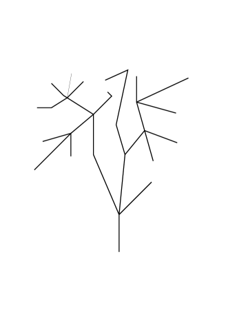
Figure 1. The tree

Every edge $e_{j}\in E$ is identified with an interval $(a_{2j-1},a_{2j})$ of the real line. The edges are connected at the vertices $v_{j}$ which can be considered as equivalence classes of the edge end points $\{a_{j}\}$. The boundary $\Gamma=\{\gamma_{1},\ldots,\gamma_{m}\}$ of $\Omega$ is a set of vertices having multiplicity one (the exterior nodes). We suppose that the each edge of the graph is equipped with the densities

(2.1) $$\frac{1}{k^{2}_{i1}},\,\frac{1}{k^{2}_{i2}}\quad\text{on $e_{i}$},\ i=1\ldots,N.$$

The densities on the edges determine the density on the graph by the rule: for $x\in e_{i}\subset\Omega\backslash V$, $\rho(x)$ is a constant which is equal to $\max{\left\{\frac{1}{k^{2}_{i1}},\,\frac{1}{k^{2}_{i2}}\right\}}$.

Since the graph under consideration is a tree, for every $a,b\in\Omega,$ $a\not=b,$ there exist the unique path $\pi[a,b]$ connecting these points. The density determines the optical metric and the optical distance

$$d\,\sigma^{2}:=\rho(x)|d\,x|^{2},\quad x\in\Omega\backslash V,$$

$$\sigma(a,b)=\int\limits_{\pi[a,\,b]}\sqrt{\rho(x)}|d\,x|,\quad a,b\in\Omega,$$

The optical diameter of the graph $\Omega$ is defined as

$$d(\Omega)=\max_{a,\,b\in\Gamma}\sigma(a,b).$$

The graph $\Omega$ and the optical metric determine the metric graph denoted by $\{\Omega,\rho\}$. For a rigorous definition of the metric graph see, e.g. [13, 14, 15, 23, 25]. The densities can also be considered as reciprocals of a stiffness parameter $k_{i1}^{2},k_{i2}^{2}$ related to a horizontal and vertical displacement $u^{i},\,w^{i}$ of an elastic string along the edge with index $i$. Each edge carries along an individual coordinate system $e_{i},\;e_{i}^{\perp}$ such that the displacement

$$r^{i}(x):=u^{i}(x)e_{i}+w^{i}(x)e_{i}^{\perp}$$

splits into a longitudinal displacement $u^{i}(x)$ and a vertical displacement $w^{i}(x)$ at the material point $x\in[a_{2i-1},a_{2i}]$. See figure 2.

Figure 2. Representation of planar displacement

The stiffness matrix can then be expressed as

$$K_{i}=k_{i1}^{2}e_{i}e_{i}^{T}+k_{i2}^{2}e_{i}^{\perp}(e_{i}^{\perp})^{T}.$$

For the sake of completeness we describe in more detail the full set of equations in more generality than we actually need later. Given a node $v_{J}$ we define

$$\mathcal{I}_{J}:=\{i\in\mathcal{I}|e_{i}\text{ is incident at }v_{J}\}$$

the incidence set, and $d_{J}=|\mathcal{I}_{J}|$ the edge degree of $v_{J}$. The set $\mathcal{J}=\{J|v_{J}\in V\}$ of node indices splits into simple nodes $\mathcal{J}_{S}$ and multiple nodes $\mathcal{J}_{M}$ according to $d_{J}=1$ and $d_{J}>1$, respectively. We introduce the subsets of boundary nodes according to tangential and vertical motions:

$$\mathcal{J}_{D}^{t}:=\{J\in\mathcal{J}_{S}|r^{i}(v_{J})\cdot e_{i}=0\}$$

$$\mathcal{J}_{D}^{n}:=\{J\in\mathcal{J}_{S}|r^{i}(v_{J})\cdot e_{i}^{\perp}=0\}$$

$$\mathcal{J}_{N}^{t}:=\{J\in\mathcal{J}_{S}|d_{iJ}K_{i}r^{i}_{x}(v_{J})\cdot e_{i}=0\}$$

$$\mathcal{J}_{N}^{n}:=\{J\in\mathcal{J}_{S}|d_{iJ}K_{i}r^{i}_{x}(v_{J})\cdot e_{i}^{\perp}=0\},$$

where

$$d_{iJ}=\begin{cases}-1&\text{ edge i starts at }v_{J}\\ 1&\text{ edge i ends at }v_{J}\end{cases},\;\;x_{iJ}=\begin{cases}0&d_{iJ}=-1\\ \ell_{i}&d_{iJ}=1.\end{cases}$$

and $r^{i}(v_{J}):=r^{i}(x_{iJ}$.

Notice that these sets are not necessarily disjoint. Obviously, the set of completely clamped vertices can be expressed as

(2.2) $$\mathcal{J}_{D}^{0}:=\mathcal{J}_{D}^{t}\cap\mathcal{J}_{D}^{n}$$

Similarly, a vertex with completely homogenous Neumann conditions is expressed as $\mathcal{J}_{N}^{n}\cap\mathcal{J}_{N}^{t}$. At tangential Dirchlet nodes in $\mathcal{J}_{D}^{t}$ we may, however, consider normal Neumann-conditions as in $\mathcal{J}_{N}^{n}$ and so on. We may then consider time dependent displacements $r^{i}(x,t)$, $t\in[0,T]$. The system of equations governing the full transient motion is then given by

(2.3) $$\left\{\begin{gathered}r^{i}_{tt}-K_{i}r^{i}_{xx}+c_{i}r^{i}=f^{i}\quad\in(0,\ell_{i})\\ r^{i}(v_{D})=u_{D},\;i\in\mathcal{I}_{D},D\in\mathcal{J}_{D}\\ d_{iJ}r^{i}_{x}(v_{N})=g_{J}\quad i\in\mathcal{I}_{N},N\in\mathcal{J}_{N}\;\\ r^{i}(v_{J})=r^{j}(v_{J})\quad i,j\in\mathcal{I}_{J},J\in\mathcal{J}_{M}\;\\ \sum\limits_{i\in\mathcal{I}_{J}}d_{iJ}K_{i}r^{i}_{x}(v_{J})=0\quad J\in\mathcal{J}_{M},\\ r^{i}(\cdot,0)=r^{i}_{0},\;{r}^{i}_{t}(\cdot,0)=r^{i}_{1}\end{gathered}\right.$$

In this representation we used capital letters for vertices in order to improve the readability of the formulae. It important to understand the coupling conditions (2.3)_4,5. Indeed, the first of these conditions simply expresses the continuity of displacements across the vertex $v_{J}$. Without this condition the network falls apart. The second condition reflects the physical law that the forces at the vertex $v_{J}$, in the absence of additional external forces acting on $v_{J}$, should add up to zero. Notice that the coupling at multiple nodes $v_{J}$, those where $|I_{J}|>1$, is a vectorial equation. This is in contrast to the out-of-the-plane model, where no such vectorial couplings occur which, in turn, makes the problem then independent of the particular geometry. In the case treated here the geometry, represented by the pairs $(e_{i},e_{i}^{\perp})$ does play a crucial role.

In Leugering and Sokolowski [22] the static system i.e. (2.3) without time-dependence, has been investigated with respect to topological sensitivities, such that the potential energy or other functionals are considered under variation of the edge-degree, nodal positions and edge-deletion. Like in this paper the analysis of the Steklov-Poincaré operators play a crucial role.

Another remark about model (2.3) is in order. If the system is static, the stiffness only active for longitudinal displacements, and if the state is edge-wise linear, then (2.3) comes down to a truss-model.

In the global Cartesian coordinate system one can represent each edge by a rotation matrix

$$R_{\alpha_{i}}=\begin{pmatrix}\cos{\alpha_{i}}&-\sin{\alpha_{i}}\\ \sin{\alpha_{i}}&\cos{\alpha_{i}}\end{pmatrix}$$

where $e_{i}=(\cos\alpha_{i},\sin\alpha_{i})^{T}$. In fact, it is the global coordinate system that we will use throughout the paper, as we are going to identify the angles $\alpha_{ij}$ between two branching edges.

2.1. Spectral settings

Let us introduce the spaces of functions on the graph $\Omega$:

(2.4) $$L_{2}(\Omega)=\bigoplus_{i=1}^{N}L_{2}(e_{i},\mathbb{R}^{2})$$

For the element $U\in L_{2}(\Omega)$ we write

(2.5) $$U=\left\{u,w\right\}=\left\{\begin{pmatrix}u^{i}\\ w^{i}\end{pmatrix}\right\}_{i=1}^{N},\quad u^{i},w^{i}\in L_{2}(e_{i}).$$

Let us consider the internal vertex $v\in V\backslash\Gamma$ and the edges $e_{1},\ldots e_{K}$ incident at $v$. We denote by $\alpha_{ij}$ the angle between two edges $e_{i}$ and $e_{j}$ counting from $e_{i}$ counterclockwise. Let $R_{\alpha}$ be the matrix corresponding to the rotation on the angle $\alpha$:

(2.6) $$R_{\alpha}=\begin{pmatrix}\cos{\alpha}&-\sin{\alpha}\\ \sin{\alpha}&\cos{\alpha}\end{pmatrix}$$

Let us introduce the matrices

(2.7) $$D^{\prime}_{i}=\begin{pmatrix}k_{i1}^{2}&0\\ 0&k_{i2}^{2}\end{pmatrix},\quad i=1,\ldots N.$$

We can now reformulate the compatibility conditions in (2.3) at multiple nodes (vertices) $v$ using global coordinates. For the sake of self-consistency in this framework we put this in the format of definitions.

Definition 1.

We say that the edge-wise continuous function $U$ satisfy the first condition (continuity) at the (multiple node) internal vertex $v$ if

(2.8) $$\begin{pmatrix}u^{i}(v)\\ w^{i}(v)\end{pmatrix}=R_{\alpha_{ij}}\begin{pmatrix}u^{j}(v)\\ w^{j}(v)\end{pmatrix},\quad 1\leqslant i,j\leqslant K,\,\,\,i\not=j.$$

Definition 2.

We say that the edge-wise continuously differentiable function $U$ satisfies the second condition (force balance) at the internal vertex $v$ if

(2.9) $$D^{\prime}_{1}\begin{pmatrix}u^{1}_{x}(v)\\ w^{1}_{x}(v)\end{pmatrix}=\sum_{j=2}^{K}R_{\alpha_{1j}}D^{\prime}_{j}\begin{pmatrix}u^{j}_{x}(v)\\ w^{j}_{x}(v)\end{pmatrix}.$$

We associate the following spectral problem to the graph:

(2.12) $$\left.\begin{array}[]{r}-k_{i1}^{2}\phi_{xx}^{i}=\lambda\phi^{i}\\ -k_{i2}^{2}\psi_{xx}^{i}=\lambda\psi^{i}\end{array}\right\}\quad x\in e_{i},\quad i=1\ldots,N,$$

(2.13) $$\left\{\phi,\psi\right\}$$ satisfies (2.8), (2.9) at all internal vertices,

(2.14) $$\left\{\phi,\psi\right\}=0\quad\text{on $\Gamma$}.$$

Definition 3.

By $\mathbf{S}$ we denote the spectral problem described by (2.12)–(2.14).

It is known that the problem $\mathbf{S}$ has a discrete spectrum of eigenvalues $0<\lambda_{1}\leqslant\lambda_{1}\leqslant\lambda_{2}\leqslant\ldots,\lambda_{k}\to\infty$. Corresponding eigenfunctions $\{\phi,\psi\}$ can be chosen such that they form an orthonormal basis in $L_{2}(\Omega).$ Indeed, for scalar problems, i.e. out-of-the-plane displacements in the mechanical context or conductivity, the spectral behavior has been explored by von Below [7], Nicaise [24] and others. The in-plane case discussed here has been treated in Lagnese, Leugering and Schmidt [16]. As a matter of fact, the spectrum consists of strings of eigenvalues coming from individual edges and strings of eigenvalues associated with the spectrum of the adjacency matrix.

2.2. Dynamical settings.

Along with the spectral, we consider dynamical system, described by the two-velocity problem on the each edge of the graph:

(2.15) $$\frac{1}{k_{i1}^{2}}u_{tt}^{i}-u_{xx}^{i}=0,\quad t>0,\ x\in e_{i}$$

(2.16) $$\frac{1}{k_{i2}^{2}}w_{tt}^{i}-w_{xx}^{i}=0,\quad t>0,\ x\in e_{i}.$$

Here the coefficients $k_{i1}$, $k_{i2}$ play the role of velocities on the edge $e_{i}$, $i=1,\ldots N$ in the first and second channels.

By $\mathcal{F}^{T}_{\Gamma}=L_{2}([0,T],\mathbb{R}^{2m})$ we denote the space of controls acting on the boundary of the tree. For the element $F\in\mathcal{F}^{T}_{\Gamma}$ we write

$$F=\{f,g\}=\left\{\begin{pmatrix}f^{i}\\ g^{i}\end{pmatrix}\right\}_{i=1}^{m},\quad f^{i},g^{i}\in L_{2}(0,T).$$

We will deal with the Dirichlet boundary conditions::

(2.17) $$\{u,w\}=\{f,g\},\quad\text{on $\Gamma\times[0,T]$}.$$

where ${f,g}\in\mathcal{F}^{T}_{\Gamma}$.

Definition 4.

By $\mathbf{D}$ we denote the dynamical problem on the graph $\Omega$, described by equations on the edges (2.15), (2.16) which satisfies compatibility conditions (2.8), (2.9) at all internal vertexes for any $t>0$, Dirichlet boundary condition (2.17) and zero initial conditions $\{u(\cdot,0),w(\cdot,0)\}=\{0,0\}$, $\{u_{t}(\cdot,0),w_{t}(\cdot,0)\}=\{0,0\}$.

It is known that for any $T>0,\ \{u,w\}\in C([0,T];L^{2}(\Omega))$. See e.g. [16, 19].

3. Inverse dynamical and spectral problems. Connection of the inverse data.

We use the Titchmarsh-Weyl (TW) matrix as the data for the inverse spectral problem. For the spectral problem on an interval and on the half line the TW function is a classical object. For the inverse spectral problem for the wave equation on trees it was used in [3, 26]. The general properties of the $M-$operator for self-adjoint operators are considered in [1, 9, 8].

Let us choose $\lambda\notin\mathbb{R}$. We define $\{\phi^{1},\psi^{1}\}$, $\{\phi^{2},\psi^{2}\}$ — two solutions of (2.12), (2.13) and the following boundary conditions:

(3.1) $$\{\phi^{1},\psi^{1}\}=\begin{pmatrix}(0,0)\\ {1}\\ (1,0)\\ (0,0)\end{pmatrix},\quad\{\phi^{2},\psi^{2}\}=\begin{pmatrix}(0,0)\\ {1}\\ (0,1)\\ (0,0)\end{pmatrix},\quad\text{on $\Gamma$},$$

where nonzero elements are located at the $i-$th row. Then the TW matrix $\mathbf{M}(\lambda)$ is defined as $\mathbf{M}(\lambda)=\{M_{ij}(\lambda)\}_{i,j=1}^{n}$ where each $M_{ij}(\lambda)$ is a $2\times 2$ matrix defined by

(3.2) $$M_{ij}(\lambda)=\begin{pmatrix}\phi^{1}_{x}(v_{j},\lambda)&\psi^{1}_{x}(v_{j},\lambda)\\ \phi^{2}_{x}(v_{j},\lambda)&\psi^{2}_{x}(v_{j},\lambda)\end{pmatrix},\quad 1\leqslant i,j\leqslant m.$$

Let us consider the nonhomogeneous Dirichlet boundary condition

(3.3) $$\{\phi,\psi\}=\{\zeta,\nu\},$$

and let $\{\phi,\psi\}$ be the solution to (2.12), (2.13), (3.3). The Titchmarsh-Weyl matrix connects the values of $\{\phi,\psi\}$ on the boundary and the values of its derivative $\{\phi_{x},\psi_{x}\}$ on the boundary:

(3.4) $$\{\phi_{x},\psi_{x}\}=\mathbf{M}(\lambda)\{\zeta,\nu\},\quad\text{on $\Gamma$}.$$

We set up the spectral inverse problem as follows: given the TW matrix $\mathbf{M}(\lambda)$, $\lambda\notin\mathbb{R}$, to recover the graph (lengths of edges, connectivity and angles between edges) and parameters of the system (2.12), i.e. the set of coefficients $\{k_{i1},k_{i2}\}_{i=1}^{N}$.

Let $\{u,w\}$ be the solution to the problem $\mathbf{D}$ with the boundary control $\{f,g\}\in\mathcal{F}^{T}_{\Gamma}$. We introduce the dynamical response operator (the dynamical Dirichlet-to-Neumann map) to the problem $\mathbf{D}$ by the rule

(3.5) $$R^{T}\{f,g\}(t)=\{u_{x}(\cdot,t),w_{x}(\cdot,t)\}\Bigl{|}_{\Gamma},\quad 0\leqslant t\leqslant T.$$

The response operator has the form of a convolution:

(3.6) $$\left(R^{T}\{f,g\}\right)\left(t\right)=\left(\mathbf{R}*\{f,g\}\right)\left(t\right),\quad 0\leqslant t\leqslant T$$

where $\mathbf{R}(t)=\{R_{ij}(t)\}_{i,j=1}^{n}$ and each $R_{i,j}(t)$ is a $2\times 2$ matrix. The entries $R_{ij}(t)$ are defined by the following procedure. We set up two dynamical problems (2.15), (2.16), (2.8), (2.9) and the boundary conditions given by

(3.7) $$\{U^{1}(\cdot,t),W^{1}(\cdot,t)\}=\begin{pmatrix}(0,0)\\ {1}\\ (\delta(t),0)\\ (0,0)\end{pmatrix},\,\,\{U^{2}(\cdot,t),W^{2}(\cdot,t)\}=\begin{pmatrix}(0,0)\\ {1}\\ (0,\delta(t))\\ (0,0)\end{pmatrix},\,\,\text{on $\Gamma$}.$$

In the above notations, the only nonzero rows is $i-$th. Then

(3.8) $$R_{ij}(t)=\begin{pmatrix}U^{1}_{x}(v_{j},t)&W^{1}_{x}(v_{j},t)\\ U^{2}_{x}(v_{j},t)&W^{2}_{x}(v_{j},t)\end{pmatrix}.$$

So, to construct the entries of $\mathbf{R}$, we need to set up the boundary condition at $i-$th boundary point in the first and second channels, while having other boundary points fixed (impose homogeneous Dirichlet conditions there) and measure the response at $j-$th boundary point in the first and second channels.

We set up the dynamical inverse problem as follows: given the response operator $R^{T}$ (3.5) (or what is equivalent, the matrix $\mathbf{R}(t)$, $t\in[0,T]$), for large enough $T,$ to recover the graph (lengths of edges, connectivity and angles between edges) and parameters for the dynamical system (2.15), (2.16), i.e. velocities on the edges.

The connection of the spectral and dynamical data is known and was used for studying the inverse spectral and dynamical problems, see for example [12, 3, 4]. Let $\{f,g\}\in\mathcal{F}^{T}_{\Gamma}\cap(C_{0}^{\infty}(0,+\infty))^{2m}$ and

$$\widehat{\{f,g\}}(k):=\int_{0}^{\infty}\{f(t),g(t)\}e^{ikt}\,dt$$

be its Fourier transform. The equations (2.15), (2.16) and (2.12) are connected by the Fourier transformation: going formally in (2.15), (2.16) over to the Fourier transform, we obtain (2.12) with $\lambda=k^{2}$. It is not difficult to check (see, e.g. [4, 3] that the response operator (response function) and Titchmarsh-Weyl matrix are connected by the same transformation:

(3.9) $$\mathbf{M}(k^{2})=\int_{0}^{\infty}\mathbf{R}(t)e^{ikt}\,dt.$$

4. Solution of the inverse problem. The case of two intervals.

We start with the inverse problem for two connected intervals. For the two-velocity system even this simple situation is nontrivial.

Suppose that a tree consists of two edges, $e_{1}$ and $e_{2}$ with the (unknown) lengths $l_{1}$ and $l_{2}$. The angle between edges we denote by $\alpha:=\alpha_{12}$ and $\Gamma=\partial\Omega=\{v_{1},v_{2}\}$ and the only internal point is $v_{3}$. We consider the dynamical problem $\mathbf{D}$ on the tree and show that we need to know response operator or TW function associated with one boundary vertex only to recover the graph.

Let us consider the problem (2.15), (2.16), (2.8), (2.9) with the boundary conditions given by

(4.1) $$\{u,w\}=\begin{pmatrix}(\delta(t),0)\\ (0,0)\end{pmatrix},\quad\text{on $\Gamma$}.$$

The solution of the above problem can be evaluated explicitly. For $0\leqslant t\leqslant\frac{l_{1}}{k_{11}}$ it is given by

$$u^{1}(x,t)=\delta\left(t-\frac{x}{k_{11}}\right),$$

$$w^{1}(x,t)=0.$$

On the time interval $\frac{l_{1}}{k_{11}}<t<\frac{2l_{2}}{\min{\{k_{21},k_{22\}}}}$ on the first edge we have

$$u^{1}(x,t)=\delta\left(t-\frac{x}{k_{11}}\right)+a_{1}\delta\left(t+\frac{x}{k_{11}}-\frac{2l_{1}}{k_{11}}\right),$$

$$w^{1}(x,t)=b_{1}\delta\left(t+\frac{x}{k_{12}}-\gamma_{12}\right),\quad\gamma_{12}=\frac{l_{1}}{k_{11}}+\frac{l_{1}}{k_{12}}.$$

and on the second edge

$$u^{2}(x,t)=a_{2}\delta\left(t-\frac{x}{k_{21}}-\gamma_{21}\right),\quad\gamma_{21}=\frac{l_{1}}{k_{11}}-\frac{l_{1}}{k_{21}},$$

$$w^{2}(x,t)=b_{2}\delta\left(t-\frac{x}{k_{22}}-\gamma_{22}\right),\quad\gamma_{22}=\frac{l_{1}}{k_{11}}-\frac{l_{1}}{k_{22}}.$$

In the formulas above, the coefficients $a_{1}$, $a_{2}$, $b_{1}$, $b_{2}$ are unknown.

¿From the condition (2.8) we obtain that

(4.2) $$\begin{pmatrix}1+a_{1}\\ b_{1}\end{pmatrix}=R_{\alpha}\begin{pmatrix}a_{2}\\ b_{2}\end{pmatrix}.$$

Condition (2.9) implies

(4.3) $$D_{1}^{\prime}\begin{pmatrix}-\frac{1}{k_{11}}+\frac{a_{1}}{k_{11}}\\ \frac{1}{k_{12}}\end{pmatrix}=R_{\alpha}D_{2}^{\prime}\begin{pmatrix}-\frac{a_{2}}{k_{21}}\\ -\frac{b2}{k_{22}}\end{pmatrix}.$$

After introducing the notation

$$D_{i}=\begin{pmatrix}k_{i1}&0\\ 0&k_{i2}\end{pmatrix},\quad i=1,\ldots N,$$

we can rewrite (4.3) as

(4.4) $$D_{1}\begin{pmatrix}-1+a_{1}\\ b_{1}\end{pmatrix}=-R_{\alpha}D_{2}\begin{pmatrix}a_{2}\\ b_{2}\end{pmatrix}.$$

Combining (4.2) and (4.4), we obtain

(4.5) $$D_{1}\begin{pmatrix}-1+a_{1}\\ b_{1}\end{pmatrix}=-R_{\alpha}D_{2}R_{-\alpha}\begin{pmatrix}1+a_{1}\\ b_{1}\end{pmatrix}.$$

Let us now consider the problem (2.15), (2.16), (2.8), (2.9) with the following boundary condition at the second channel:

(4.6) $$\{u,v\}=\begin{pmatrix}(0,\delta(t))\\ (0,0)\end{pmatrix},\quad\text{on $\Gamma$}.$$

The computations similar to ones for the case of the boundary condition at the first channel show that the following condition must hold:

(4.7) $$D_{1}\begin{pmatrix}\widetilde{b}_{1}\\ -1+\widetilde{a}_{1}\end{pmatrix}=-R_{\alpha}D_{2}R_{-\alpha}\begin{pmatrix}\widetilde{b}_{1}\\ 1+\widetilde{a}_{1}\end{pmatrix},$$

where the coefficients $\widetilde{a}_{1}$, $\widetilde{a}_{2}$, $\widetilde{b}_{1}$, $\widetilde{b}_{2}$ are unknown.

The function $u^{1}(x,t)$, the first component of the solution to (2.15), (2.16), (2.8), (2.9), (4.1) has the following representation on the time interval $\frac{2l_{1}}{k_{11}}<t<\frac{2l_{1}}{k_{11}}+2\min_{i,j}\{\frac{l_{i}}{k_{ij}}\}$

(4.8) $$u^{1}(x,t)=\delta\left(t-\frac{x}{k_{11}}\right)+a_{1}\delta\left(t+\frac{x}{k_{11}}-\frac{2l_{1}}{k_{11}}\right)-a_{1}\delta\left(t-\frac{x}{k_{11}}-\frac{2l_{1}}{k_{11}}\right)$$

Thus (see the definition of the response operator (3.8)) for such $t$:

(4.9) $$\{R_{11}\}_{11}(t)=u^{1}_{x}(0,t)=-\frac{1}{k_{11}}\delta^{\prime}(t)+\frac{2a_{1}}{k_{11}}\delta^{\prime}\left(t-\frac{2l_{1}}{k_{11}}\right).$$

A similar argument shows that for $\frac{l_{1}}{k_{11}}+\frac{l_{1}}{k_{12}}<t<\frac{l_{1}}{k_{11}}+\frac{l_{1}}{k_{12}}+2\min_{i,j}\{\frac{l_{i}}{k_{ij}}\}$

(4.10) $$\{R_{11}\}_{12}(t)=w^{1}_{x}(0,t)=2\frac{b_{1}}{k_{12}}\delta^{\prime}\left(t-\gamma_{12}\right).$$

Thus using the $\{R_{11}\}_{12}$, $\{R_{11}\}_{12}$ components of the response operator on the described time intervals, we can determine $k_{11}$, $k_{12}$, $a_{1}$, $b_{1}$, $l_{1}$. Applying the same argument to the problem (2.15), (2.16), (2.8), (2.9), (4.6), we conclude that $\{R_{11}\}_{21}$, $\{R_{11}\}_{22}$ components of the response function determine $\widetilde{a}_{1}$, $\widetilde{b}_{1}$.

Let us introduce the notations

$$\xi_{1}=1+a_{1},\quad\eta_{1}=b_{1},$$

$$\widetilde{\xi}_{1}=\widetilde{b}_{1},\quad\widetilde{\eta}_{1}=1+\widetilde{a}_{1},$$

and rewrite (4.5), (4.7) as

(4.11) $$\left(R_{\alpha}D_{2}R_{-\alpha}+D_{1}\right)\begin{pmatrix}\xi_{1}\\ \eta_{1}\end{pmatrix}=2D_{1}\begin{pmatrix}1\\ 0\end{pmatrix},$$

(4.12) $$\left(R_{\alpha}D_{2}R_{-\alpha}+D_{1}\right)\begin{pmatrix}\widetilde{\xi}_{1}\\ \widetilde{\eta}_{1}\end{pmatrix}=2D_{1}\begin{pmatrix}0\\ 1\end{pmatrix}.$$

In the forward problem, the equations (4.11) and (4.12) can be used for the determination of the reflection and transmission coefficients $a_{1}$, $b_{1}$, $\widetilde{a}_{1}$, $\widetilde{b}_{1}$. Since the (given) matrixes $R_{\alpha}D_{2}R_{-\alpha}+D_{1}$ and $D_{1}$ are positive definite (it is easy to check that $R_{\alpha}D_{j}R_{-\alpha}\geqslant\min\{k_{j1},k_{j2}\}I$), these coefficients are uniquely determined from (4.11), (4.12). Moreover, we necessarily have

(4.13) $$\begin{pmatrix}\xi_{1}\\ \eta_{1}\end{pmatrix}\not=\begin{pmatrix}\widetilde{\xi}_{1}\\ \widetilde{\eta}_{1}\end{pmatrix}$$

On the other hand, in the inverse problem we know $D_{1}$, $\xi_{1}$, $\eta_{1}$, $\widetilde{\xi}_{1}$, $\widetilde{\eta}_{1}$ (we can determine all these coefficients from $R_{11}$ component of the response operator). Thus equations (4.11), (4.12) determine the matrix $A=R_{\alpha}D_{2}R_{-\alpha}$. Using the invariants of matrix — the determinant and trace, we can find the matrix $D_{2}$ from the equations

(4.14) $$k_{21}+k_{22}=\operatorname{tr}{A},\quad k_{21}k_{22}=\det{A}.$$

The existence of angle $\alpha$ follows from the spectral theorem — $R_{\alpha}$ “diagonalize” operator $A$.

Notice that if $D_{2}=\gamma I,$ there is no dependence on $\alpha$ in equations (4.11), (4.12).

We point out that we still need to determine the length of the second edge. For this aim we could analyze the representation of the solutions $u^{1}$, $w^{1}$ on a sufficiently large time interval. It would lead to an increasing number of terms in (4.8) and (4.9), (4.10). Instead of that we will develop the method which works for general trees following ideas of [3]. Let us consider the new tree, consisting of one edge: $\widetilde{\Omega}=e_{2}$. Idea of the method is to recalculate the TW matrix for the new tree using the TW matrix and response operator for the whole tree $\Omega$ and the data that we obtained on the first step, i.e. parameters of the first edge and the angle between edges.

Let $\{U,W\}$ be the solution of (2.12), (2.13) on $\Omega$ with boundary conditions

(4.15) $$\{U,W\}=\{\zeta,\nu\},\,\,\text{at $v_{1}$},\quad\{U,W\}=\{0,0\},\,\,\text{at $v_{2}$}.$$

The compatibility conditions at the internal vertex $v_{3}$ are:

(4.16) $$\begin{pmatrix}U^{1}(v_{3},\lambda)\\ W^{1}(v_{3},\lambda)\end{pmatrix}=R_{\alpha}\begin{pmatrix}U^{2}(v_{3},\lambda)\\ W^{2}(v_{3},\lambda)\end{pmatrix},$$

(4.17) $$D^{\prime}_{1}\begin{pmatrix}U^{1}_{x}(v_{3},\lambda)\\ W^{1}_{x}(v_{3},\lambda)\end{pmatrix}=R_{\alpha}D^{\prime}_{2}\begin{pmatrix}U^{2}_{x}(v_{3},\lambda)\\ W^{2}_{x}(v_{3},\lambda)\end{pmatrix}.$$

Let $\widetilde{M}(\lambda)$ be the TW matrix for the tree $\widetilde{\Omega}$. We see that $\widetilde{M}_{11}(\lambda)$ – component associated with the “new” boundary point $v_{3}$ satisfies equation:

(4.18) $$\begin{pmatrix}U^{2}_{x}(v_{3},\lambda)\\ W^{2}_{x}(v_{3},\lambda)\end{pmatrix}=\widetilde{M}_{11}(\lambda)\begin{pmatrix}U^{2}(v_{3},\lambda)\\ W^{2}(v_{3},\lambda)\end{pmatrix}.$$

¿From (4.16)–(4.18) it follows

(4.19) $$D^{\prime}_{1}\begin{pmatrix}U^{1}_{x}(v_{3},\lambda)\\ W^{1}_{x}(v_{3},\lambda)\end{pmatrix}=R_{\alpha}D^{\prime}_{2}\widetilde{M}_{11}(\lambda)R_{-\alpha}\begin{pmatrix}U^{1}(v_{3},\lambda)\\ W^{1}(v_{3},\lambda)\end{pmatrix}.$$

We emphasize that in (4.19) we know everything but the matrix $\widetilde{M}(\lambda)$. Choosing different boundary conditions for the problem in (4.15), we can get linear independent vectors $\begin{pmatrix}U^{1}(v_{3},\lambda)\\ W^{1}(v_{3},\lambda)\end{pmatrix}$ in (4.19). Thus (4.19) determines the matrix $\widetilde{M}_{11}(\lambda)$. The matrix $\widetilde{M}_{11}$ uniquely determines the corresponding component of the response operator $\widetilde{R}_{11}$ (see (3.9)). The latter operator in turn, allows us to find the parameters of the second edge, exactly as $R_{11}$ determines the parameters of the first edge. (In our simple case of the two edge tree, the only parameter which we need to recover is the length of the second edge.)

We conclude the results of the present section in the following statement

Theorem 1.

Let $\Omega$ be the tree consisted of two edges. Then the tree and the parameters of the systems (2.15), (2.16) and (2.12) are determined by the $2\times 2$ matrix $M_{11}(\lambda)$ the diagonal element of the TW matrix, associated with the first boundary point.

In the remaining part of the paper we will deal with the dynamical approach to the inverse problem. We will prove the following statement:

Remark 1.

The $2\times 2$ matrix $R_{11}(t)$ for $t\in[0,T]$ where $T>2d(\Omega)$ determines the tree and the parameters of the systems (2.15), (2.16) and (2.12)

5. Solution of the inverse problem. The case of a star graph.

Suppose that the tree is a star graph with edges $e_{1},\ldots e_{n}$, $e_{i}=[z_{i},z_{0}]$, $i=1,\ldots n$. To recover the graph and the parameters of the system (2.15), (2.16) we use the diagonal elements of the response operator (or diagonal elements of the Weil matrix), associated to the boundary vertices $z_{1},\ldots z_{n-1}$.

Let us set up the initial-value problem (2.15), (2.16), (2.8), (2.9) with the boundary conditions given by the first equation in (3.7). We suppose that the only nonzero boundary conditions are given at the first channel of the $i-th$ boundary vertex, $i\not=n$. Analyzing the solution $\{u,w\}$ of these problems in a way we did for the case of the graph of two edges, we obtain that on the time interval $\frac{l_{i}}{k_{i1}}<t<\frac{l_{i}}{k_{i1}}+2\min_{i,j}\{\frac{l_{i}}{k_{ij}}\}$ on the $i-$th edge we have

$$u^{i}(x,t)=\delta\left(t-\frac{x}{k_{i1}}\right)+a^{i}_{i}\delta\left(t+\frac{x}{k_{i1}}-\frac{2l_{i}}{k_{i1}}\right),$$

$$w^{i}(x,t)=b^{i}_{i}\delta\left(t+\frac{x}{k_{i2}}-\gamma_{i2}\right),\quad\gamma_{i2}=\frac{l_{i}}{k_{i1}}+\frac{l_{i}}{k_{i2}}.$$

and on other edges ($j=1\ldots n$, $j\not=i$):

$$u^{j}(x,t)=a^{i}_{j}\delta\left(t-\frac{x}{k_{j1}}-\gamma_{j1}\right),\quad\gamma_{j1}=\frac{l_{i}}{k_{i1}}-\frac{l_{i}}{k_{j1}},$$

$$w^{j}(x,t)=b^{i}_{j}\delta\left(t-\frac{x}{k_{j2}}-\gamma_{j2}\right),\quad\gamma_{j2}=\frac{l_{i}}{k_{i1}}-\frac{l_{i}}{k_{j2}}.$$

Where $a^{i}_{j}$, $b^{i}_{j}$, $i=1,\ldots,n-1$, $j=1,\ldots,n$ are reflection and transmission coefficients associated with the $i-th$ vertex. Let us introduce new parameters

(5.1) $$\xi_{i}=1+a^{i}_{i},\quad\eta_{i}=b^{i}_{i},\quad i=1,\ldots,n-1.$$

The compatibility conditions (2.8), (2.9) at the internal vertex $z_{0}$ (we need to rewrite them in a way we did for the case of two edges) lead to the following equalities (cf. (4.11)):

(5.2) $$\left(\sum_{j\not=i}R_{\alpha_{ij}}D_{j}R_{-\alpha_{ij}}+D_{i}\right)\begin{pmatrix}\xi_{i}\\ \eta_{i}\end{pmatrix}=2D_{i}\begin{pmatrix}1\\ 0\end{pmatrix},\quad i=1,\ldots n-1.$$

Let us now set up the initial-value problem with the delta function in the second channel at $i-$th boundary point, $i\not=n$, which is given by (2.15), (2.16), (2.8), (2.9) and the boundary conditions given by the second equation in (3.7). We can obtain and analyze the representation for the solutions $\{\widetilde{u},\widetilde{w}\}$ of these problems. Let $\widetilde{a}_{i}$, $\widetilde{b}_{i}$, $i=1,\ldots,n-1$, $j=1,\ldots,n$ be the reflection and transmission coefficients. Introducing new parameters

(5.3) $$\widetilde{\xi}_{i}=\widetilde{b}^{i}_{i},\quad\widetilde{\eta}_{i}=1+\widetilde{a}^{i}_{i},\quad i=1,\ldots n-1$$

and making use of the compatibility conditions (2.8), (2.9) at the internal vertex $z_{0}$, we obtain the following equalities (cf. (4.12)):

(5.4) $$\left(\sum_{j\not=i}R_{\alpha_{ij}}D_{j}R_{-\alpha_{ij}}+D_{i}\right)\begin{pmatrix}\widetilde{\xi}_{i}\\ \widetilde{\eta}_{i}\end{pmatrix}=2D_{i}\begin{pmatrix}0\\ 1\end{pmatrix},\quad i=1,\ldots n-1.$$

The matrices $\left(\sum_{j\not=i}R_{\alpha_{ij}}D_{j}R_{-\alpha_{ij}}+D_{i}\right)$, $i=1,\ldots,n-1$ are positive definite. If all angles between edges and all matrices $D_{j}$ are known, the systems (5.2), (5.4) can be solved for $\xi_{i}$, $\eta_{i}$, $\widetilde{\xi}_{i}$, $\widetilde{\eta}_{i}$. Note that necessarily

$$\begin{pmatrix}\widetilde{\xi}_{i}\\ \widetilde{\eta}_{i}\end{pmatrix}\not=\begin{pmatrix}\xi_{i}\\ \eta_{i}\end{pmatrix},\quad i=1,\ldots n-1.$$

In the situation of the inverse problem, using the diagonal elements $\{R_{ii}\}$, $i=1,\ldots,n-1$ of the response operator, we can determine the reflection and transmission coefficients $a^{i}_{i}$, $b^{i}_{i}$, $\widetilde{a}^{i}_{i}$, $\widetilde{b}^{i}_{i}$, as well as $l_{i}$, $D_{i}$ for $i=1,\ldots,n-1$. Indeed: analyzing the solution to the dynamical system $\mathbf{D}$ with the boundary condition given by the delta function in the first channel at the $i-$th boundary vertex, it is easy to see (cf. (4.9), (4.10)) that:

$$\{R_{ii}\}_{11}(t)={u^{i}}_{x}(0,t)=-\frac{1}{k_{i1}}\delta^{\prime}(t)+\frac{2a^{i}_{i}}{k_{i1}}\delta^{\prime}\left(t-\frac{2l_{i}}{k_{i1}}\right),$$

$$\quad\frac{2l_{i}}{k_{i1}}<t<\frac{2l_{i}}{k_{i1}}+2\min_{i,j}\{\frac{l_{i}}{k_{ij}}\},$$

$$\{R_{ii}\}_{12}(t)={w^{i}}_{x}(0,t)=\frac{b^{i}_{i}}{k_{i2}}\delta^{\prime}\left(t-\gamma_{i2}\right),$$

$$\quad\gamma_{i2}<t<\gamma_{i2}+2\min_{i,j}\{\frac{l_{i}}{k_{ij}}\}.$$

The above representation allows one to determine $a^{i}_{i}$, $b^{i}_{i}$, $l_{i}$, $k_{i1}$ for $i=1,\ldots,n-1$. Analyzing the solutions to the dynamical system $\mathbf{D}$ with the boundary condition given by the delta function at the second channel of the $i-$th boundary vertex, we can determine $\widetilde{a}^{i}_{i}$, $\widetilde{b}^{i}_{i}$, $k_{i2}$ for $i=1,\ldots,n-1$.

Thus, since the vectors $\begin{pmatrix}\widetilde{\xi}_{i}\\ \widetilde{\eta}_{i}\end{pmatrix}$ and $\begin{pmatrix}\xi_{i}\\ \eta_{i}\end{pmatrix}$ in (5.2), (5.4) are known and necessarily different, equations (5.2), (5.4) completely determines the matrixes $A_{i}$,

(5.5) $$A_{i}=\sum_{j\not=i}R_{\alpha_{ij}}D_{j}R_{-\alpha_{ij}}+D_{i},\quad i=1\ldots n.$$

In (5.5) we do not know $n-1$ angles between edges and the matrix $D_{n}$. We use the system (5.5) to determine them in the same way we did it for the case of two intervals, but calculations are more involved.

Let us consider the condition (5.5) for $i=k$ and for $i=l$:

(5.6) $$D_{k}+R_{\alpha_{kl}}D_{l}R_{-\alpha_{kl}}+\sum_{j\not=k,\,l}R_{\alpha_{kj}}D_{j}R_{-\alpha_{kj}}=A_{k},$$

(5.7) $$D_{l}+R_{\alpha_{lk}}D_{k}R_{-\alpha_{lk}}+\sum_{j\not=k,\,l}R_{\alpha_{lj}}D_{j}R_{-\alpha_{lj}}=A_{l},$$

where the matrices $A_{k}$ and $A_{l}$ are known. Note that after the multiplication of (5.7) by $R_{\alpha_{kl}}$ from the left and by $R_{-\alpha_{kl}}$ from the right, and using that $R_{\alpha_{kl}}=R_{-\alpha_{lk}}$, $R_{\alpha_{kl}}R_{\alpha_{lj}}=R_{\alpha_{kj}}$, we obtain

$$A_{k}=R_{\alpha_{kl}}A_{l}R_{-\alpha_{kl}}.$$

The angle $\alpha_{kl}$ can now be found using the spectral theorem. Repeating this procedure for various $i$, $l$ we can determine all angles. After that we can use any of the conditions (5.5) to determine $D_{n}$. Indeed, taking $i=k$ we have

(5.8) $$R_{\alpha_{kn}}D_{n}R_{-\alpha_{kn}}=B_{k}$$

for some known matrix $B_{k}$. Then

(5.9) $$k_{n1}+k_{n2}=\operatorname{tr}{B_{k}},\quad k_{n1}k_{n2}=\det{B_{k}}.$$

The next step is crucial for solving the inverse problem: we have already recovered a part of the tree, and our next aim is to find the inverse data for the smaller “new” tree, using the initial inverse data and information that we obtained on the previous steps.

Let us consider the new tree, consisting of the one edge $\widetilde{\Omega}=e_{n}=[z_{0},z_{n}]$. By $\{\Phi,\Psi\}$ we denote the solution to (2.12), (2.13) and the following boundary conditions

(5.10) $$\{\Phi,\Psi\}=\{\zeta,\nu\},\,\,\text{at $z_{1}$},\quad\{\Phi,\Psi\}=\{0,0\},\,\,\text{at $z_{i},\,\,2\leqslant i\leqslant n$}.$$

As in the case of a graph consisting of two intervals, our goal is to obtain the coefficient $\widetilde{M}_{11}$ of the TW-matrix for $\widetilde{\Omega}$, associated with the “new” boundary edge $z_{0}$. Note that we can assume that we have already recovered the information about all other edges and angles between them. So we have in hands the matrices $D_{i}^{\prime}$, and $\alpha_{i,n}$ for $i=1,\ldots n$.

Note that solution to 2.12), (2.13), (5.10) on the edge $e_{1}$ solves the Cauchy problem

(5.11) $$-k_{11}^{2}\Phi_{xx}^{1}=\lambda\Phi^{1},\quad-k_{12}^{2}\Psi_{xx}^{1}=\lambda\Psi^{1},\quad x\in e_{1}$$

(5.12) $$\{\Phi^{1}(z_{1}),\Psi^{1}(z_{1})\}=\{\zeta,\nu\},$$

(5.13) $$\begin{pmatrix}\Phi^{1}_{x}(z_{1})\\ \Psi^{1}_{x}(z_{1})\end{pmatrix}=\{M_{11}(\lambda)\}\begin{pmatrix}\zeta\\ \nu\end{pmatrix},$$

and on edges $e_{2},\ldots,e_{n-1}$ solves the Cauchy problems

(5.14) $$-k_{i1}^{2}\Phi_{xx}^{i}=\lambda\Phi^{i},\quad-k_{i2}^{2}\Psi_{xx}^{i}=\lambda\Psi^{i},\quad x\in e_{i}$$

(5.15) $$\{\Phi^{1}(z_{i}),\Psi^{1}(z_{i})\}=\{0,0\},$$

(5.16) $$\begin{pmatrix}\Phi^{i}_{x}(z_{i})\\ \Psi^{i}_{x}(z_{i})\end{pmatrix}=\{M_{1i}(\lambda)\}\begin{pmatrix}\zeta\\ \nu\end{pmatrix}.$$

Thus the function $\{\Phi,\Psi\}$ and its derivative is known on the edges $e_{1},\ldots,e_{n-1}$. At the internal vertex $z_{0}$ compatibility conditions hold:

(5.17) $$\begin{pmatrix}\Phi^{1}(z_{0},\lambda)\\ \Psi^{1}(z_{0},\lambda)\end{pmatrix}=R_{\alpha_{in}}\begin{pmatrix}\Phi^{n}(z_{0},\lambda)\\ \Psi^{n}(z_{0},\lambda)\end{pmatrix},$$

(5.18) $$D^{\prime}_{1}\begin{pmatrix}\Phi^{1}_{x}(z_{0},\lambda)\\ \Psi^{1}_{x}(z_{0},\lambda)\end{pmatrix}=\sum_{j\not=1,n}R_{\alpha_{1j}}D^{\prime}_{j}\begin{pmatrix}\Phi^{j}_{x}(z_{0},\lambda)\\ \Psi^{j}_{x}(z_{0},\lambda)\end{pmatrix}+R_{\alpha_{1n}}D^{\prime}_{n}\begin{pmatrix}\Phi^{n}_{x}(z_{0},\lambda)\\ \Psi^{n}_{x}(z_{0},\lambda)\end{pmatrix}.$$

Using these conditions and the definition of the component of TW-matrix associated with the $n-$th edge:

(5.19) $$\begin{pmatrix}\Phi^{n}_{x}(z_{0},\lambda)\\ \Psi^{n}_{x}(z_{0},\lambda)\end{pmatrix}=\widetilde{M}_{11}(\lambda)\begin{pmatrix}\Phi^{n}(z_{0},\lambda)\\ \Psi^{n}(z_{0},\lambda)\end{pmatrix},$$

we get the equations

(5.20) $$D^{\prime}_{i}\begin{pmatrix}\Phi^{1}_{x}(z_{0},\lambda)\\ \Psi^{1}_{x}(z_{0},\lambda)\end{pmatrix}=\sum_{j\not=1,n}R_{\alpha_{1j}}D^{\prime}_{j}\begin{pmatrix}\Phi^{j}_{x}(z_{0},\lambda)\\ \Psi^{j}_{x}(z_{0},\lambda)\end{pmatrix}+$$

$$R_{\alpha_{1n}}D^{\prime}_{n}\widetilde{M}_{11}(\lambda)R_{-\alpha_{1n}}\begin{pmatrix}\Phi^{1}(z_{0},\lambda)\\ \Psi^{1}(z_{0},\lambda)\end{pmatrix}.$$

Choosing the different boundary conditions at the $i-$th boundary point, we can get vectors $\begin{pmatrix}\Phi^{i}(z_{0},\lambda)\\ \Psi^{i}(z_{0},\lambda)\end{pmatrix}$ in (5.20) to be linearly independent. Since we know all other terms in (5.20), this equation determines $\widetilde{M}_{11}(\lambda)$. Using the connection of the dynamical and spectral data (3.9), we can recover the $\widetilde{R}_{11}$ component of the response function associated with $\widetilde{\Omega}$ and reduce our problem to the inverse problem for one edge. (Really we still need to recover only the length of the $n-$th edge.)

We combine all results of this section in

Theorem 2.

Let $\Omega$ be the a star graph consisted of $n$ edges. Then the graph and the parameters of the systems (2.15), (2.16) and (2.12), are determined by the diagonal elements ($2\times 2$ matrices) $M_{ii}(\lambda)$ $1\leqslant i\leqslant n-1$ of the $TM$ matrix.

We proceed to prove the following statement:

Remark 2.

The diagonal elements ($2\times 2$ matrices) $R_{ii}(t)$ $1\leqslant i\leqslant n-1$ of the response function for $t>d(\Omega)$ determine the tree and the parameters of the systems (2.15), (2.16) and (2.12)

6. Solution of the inverse problem. The case of an arbitrary tree.

Let $\Omega$ be a finite tree with $m$ boundary points $\Gamma=\{\gamma_{1},\ldots,\gamma_{m}\}$. Without loss of generality we can assume that the boundary vertex $\gamma_{m}$ is a root of the tree. We consider the dynamical problem $\mathbf{D}$ and the spectral problem $\mathbf{S}$ on $\Omega$. Then the response function $\mathbf{R}(t)=\{R_{ij}(t)\}_{i,j=1}^{m-1}$ and the TW matrix $\mathbf{M}(\lambda)=\{M_{ij}(\lambda)\}_{i,j=1}^{m-1}$ associated with all other boundary points are constructed in the same way as in the section 3.

Let us take two boundary edges, $e_{i}$ with the length $l_{i}$ and velocities in channels $k_{i1}$, $k_{i2}$ and $e_{j}$ with the length $l_{j}$ and velocities in channels $k_{j1}$, $k_{j2}$. These two edges have one common point if and only if

(6.1) $$\{R_{ij}\}_{11}(t)=\left\{\begin{array}[]{l}=0,\quad\text{for $t<\frac{l_{i1}}{k_{i1}}+\frac{l_{j1}}{k_{j1}}$}\\ \not=0,\quad\text{for $t>\frac{l_{i1}}{k_{i1}}+\frac{l_{j1}}{k_{j1}}$}\end{array}\right.,\quad 1\leqslant i,j\leqslant m-1.$$

Note that one can use other components of $R_{ij}$ to determine the connectivity of edges.

This method allows us to divide the boundary edges into groups, such that edges from one group have a common vertex. Let us take the first of such groups, say $e_{1}=[z_{1},z_{0}],\ldots,e_{m_{0}}=[z_{m_{0}},z_{0}]$ with boundary vertices $\gamma_{1},\ldots,\gamma_{m_{0}}$. These edges together with another edge $e=[z_{0},z_{m_{0}^{\prime}}]$ form a star graph, the subgraph of $\Omega$. Note, that using the diagonal elements of the response operator $\{R_{ii}(t)\}$ or the diagonal elements of the TW-matrix $M(\lambda)$, $i=1,\ldots,m_{0}$ by the same method as in the case of star graph, we can determine angles and velocities for all edges $e_{1},\ldots,e_{m_{0}},[z_{0},z_{m_{0}^{\prime}}]$ and lengths all boundary edges $e_{1},\ldots,e_{m_{0}}$.

We take the new tree $\widetilde{\Omega}=\Omega\backslash\bigcup_{i=1}^{m_{0}}e_{i}$. Our goal as in the previous cases is to calculate $\widetilde{M}(\lambda)$, the TW-matrix associated with $\widetilde{\Omega}$.

By $\{\Phi,\Psi\}$ we denote the solution to (2.12), (2.13) and the following boundary conditions

(6.2) $$\{\Phi,\Psi\}=\{\zeta,\nu\},\,\,\text{at $\gamma_{1}$},\quad\{\Phi,\Psi\}=\{0,0\},\,\,\text{at $\gamma_{i},\,\,2\leqslant i\leqslant m$}.$$

Note that the solution to (2.12), (2.13), (6.2) on the edge $e_{1}$ solves the Cauchy problem

(6.3) $$-k_{11}^{2}\Phi_{xx}^{1}=\lambda\Phi^{1},\quad-k_{12}^{2}\Psi_{xx}^{1}=\lambda\Psi^{1},\quad x\in e_{1}$$

(6.4) $$\{\Phi^{1}(z_{1}),\Psi^{1}(z_{1})\}=\{\zeta,\nu\},$$

(6.5) $$\begin{pmatrix}\Phi^{1}_{x}(z_{1})\\ \Psi^{1}_{x}(z_{1})\end{pmatrix}=\{M_{11}(\lambda)\}\begin{pmatrix}\zeta\\ \nu\end{pmatrix},$$

and on the edges $e_{2},\ldots,e_{m_{0}}$ solves

(6.6) $$-k_{i1}^{2}\Phi_{xx}^{i}=\lambda\Phi^{i},\quad-k_{i2}^{2}\Psi_{xx}^{i}=\lambda\Psi^{i},\quad x\in e_{i}$$

(6.7) $$\{\Phi^{i}(z_{i}),\Psi^{i}(z_{i})\}=\{0,0\},$$

(6.8) $$\begin{pmatrix}\Phi^{i}_{x}(z_{i})\\ \Psi^{i}_{x}(z_{i})\end{pmatrix}=\{M_{1i}(\lambda)\}\begin{pmatrix}\zeta\\ \nu\end{pmatrix}.$$

Thus the function $\{\Phi,\Psi\}$ and its derivative is known on edges $e_{1},\ldots,e_{m_{0}}$.

At the internal vertex $z_{0}$ compatibility conditions hold:

(6.9) $$\begin{pmatrix}\Phi^{1}(z_{0},\lambda)\\ \Psi^{1}(z_{0},\lambda)\end{pmatrix}=R_{\alpha_{1m_{0}^{\prime}}}\begin{pmatrix}\Phi^{m_{0}^{\prime}}(z_{0},\lambda)\\ \Psi^{m_{0}^{\prime}}(z_{0},\lambda)\end{pmatrix},$$

(6.10) $$D^{\prime}_{1}\begin{pmatrix}\Phi^{1}_{x}(z_{0},\lambda)\\ \Psi^{1}_{x}(z_{0},\lambda)\end{pmatrix}=\sum_{j\not=1,m_{0}^{\prime}}R_{\alpha_{1j}}D^{\prime}_{j}\begin{pmatrix}\Phi^{j}_{x}(z_{0},\lambda)\\ \Psi^{j}_{x}(z_{0},\lambda)\end{pmatrix}+$$

$$R_{\alpha_{1m_{0}^{\prime}}}D^{\prime}_{m_{0}^{\prime}}\begin{pmatrix}\Phi^{m_{0}^{\prime}}_{x}(z_{0},\lambda)\\ \Psi^{m_{0}^{\prime}}_{x}(z_{0},\lambda)\end{pmatrix}.$$

Using these conditions and the definition of the TW-matrix associated with the $m_{0}^{\prime}-$th edge:

(6.11) $$\begin{pmatrix}\Phi^{m_{0}^{\prime}}_{x}(z_{0},\lambda)\\ \Psi^{m_{0}^{\prime}}_{x}(z_{0},\lambda)\end{pmatrix}=\widetilde{M}_{{m_{0}^{\prime}}{m_{0}^{\prime}}}(\lambda)\begin{pmatrix}\Phi^{m_{0}^{\prime}}(z_{0},\lambda)\\ \Psi^{m_{0}^{\prime}}(z_{0},\lambda)\end{pmatrix},$$

we obtain that

(6.12) $$D^{\prime}_{1}\begin{pmatrix}\Phi^{1}_{x}(z_{0},\lambda)\\ \Psi^{1}_{x}(z_{0},\lambda)\end{pmatrix}=\sum_{j=2}^{m_{0}^{\prime}}R_{\alpha_{1j}}D^{\prime}_{j}\begin{pmatrix}\Phi^{j}_{x}(z_{0},\lambda)\\ \Psi^{j}_{x}(z_{0},\lambda)\end{pmatrix}+$$

$$R_{\alpha_{1{m_{0}^{\prime}}}}D^{\prime}_{m_{0}^{\prime}}\widetilde{M}_{{m_{0}^{\prime}}{m_{0}^{\prime}}}(\lambda)R_{-\alpha_{1{m_{0}^{\prime}}}}\begin{pmatrix}\Phi^{1}(z_{0},\lambda)\\ \Psi^{1}(z_{0},\lambda)\end{pmatrix}.$$

Equation (6.12) determines the matrix $\widetilde{M}_{{m_{0}^{\prime}}{m_{0}^{\prime}}}(\lambda)$. By definition of the TW-matrix we have

(6.13) $$\{M_{1j}(\lambda)\}\begin{pmatrix}\zeta\\ \nu\end{pmatrix}=\begin{pmatrix}\Phi^{j}(e_{j})\\ \Psi^{j}(e_{j})\end{pmatrix},\quad m_{0}<j<m.$$

On the other hand, by the definition for the TW-matrix for the new tree $\widetilde{\Omega}$,

(6.14) $$\begin{pmatrix}\Phi^{j}(e_{j})\\ \Psi^{j}(e_{j})\end{pmatrix}=\{\widetilde{M}_{m_{0}^{\prime}j}(\lambda)\}\begin{pmatrix}\Phi^{m_{0}^{\prime}}(z_{0})\\ \Psi^{m_{0}^{\prime}}(z_{0})\end{pmatrix},\quad m_{0}<j<m.$$

Thus $\{\widetilde{M}_{m_{0}^{\prime}j}(\lambda)\}$ component of the TW matrix can be found from the equation

(6.15) $$\{\widetilde{M}_{m_{0}^{\prime}j}(\lambda)\}\begin{pmatrix}\Phi^{m_{0}^{\prime}}(z_{0})\\ \Psi^{m_{0}^{\prime}}(z_{0})\end{pmatrix}=\{M_{1j}(\lambda)\}\begin{pmatrix}\zeta\\ \nu\end{pmatrix},\quad m_{0}<j<m.$$

To find the components $\widetilde{M}_{im_{0}^{\prime}}(\lambda)$, $m_{0}<i<m$, we fix $\gamma_{i}$ and denote by $\{\Phi,\Psi\}$ the solution to (2.12), (2.13) with the boundary conditions

(6.16) $$\{\Phi,\Psi\}=\{\zeta,\nu\},\,\,\text{at $\gamma_{i}$},\quad\{\Phi,\Psi\}=\{0,0\},\,\,\text{at $\gamma_{j},\,\,j\not=i$}.$$

Note that on the edges $e_{1},\ldots,e_{m_{0}}$ $\{\Phi,\Psi\}$ satisfies the equations

(6.17) $$-k_{j1}^{2}\Phi_{xx}^{j}=\lambda\Phi^{j},\quad-k_{j2}^{2}\Psi_{xx}^{j}=\lambda\Psi^{j},\quad x\in e_{j}$$

(6.18) $$\{\Phi^{j}(z_{j}),\Psi^{j}(z_{j})\}=\{0,0\},$$

(6.19) $$\begin{pmatrix}\Phi^{j}_{x}(z_{j})\\ \Psi^{j}_{x}(z_{j})\end{pmatrix}=\{M_{ij}(\lambda)\}\begin{pmatrix}\zeta\\ \nu\end{pmatrix}.$$

Thus, the function $\{\Phi,\Psi\}$ and its derivative are known on the edges $e_{1},\ldots,e_{m_{0}}$. Using the compatibility conditions at the internal vertex $z_{0}$, for every $\begin{pmatrix}\zeta\\ \nu\end{pmatrix}$ we can find the vectors $\begin{pmatrix}\Phi^{m_{0}^{\prime}}(z_{0},\lambda)\\ \Psi^{m_{0}^{\prime}}(z_{0},\lambda)\end{pmatrix}$, $\begin{pmatrix}\Phi^{m_{0}^{\prime}}_{x}(z_{0},\lambda)\\ \Psi^{m_{0}^{\prime}}_{x}(z_{0},\lambda)\end{pmatrix}$. We emphasize that the function $\{\Phi,\Psi\}$ does not satisfy zero Dirichlet conditions at $z_{0}$. Components $\widetilde{M}_{im_{0}^{\prime}}(\lambda)$, $i=m_{0}+1,\ldots,m$ can be obtained from the equations

(6.20) $$\begin{pmatrix}\Phi^{m_{0}^{\prime}}_{x}(z_{0},\lambda)\\ \Psi^{m_{0}^{\prime}}_{x}(z_{0},\lambda)\end{pmatrix}-\widetilde{M}_{m_{0}^{\prime}m_{0}^{\prime}}(\lambda)\begin{pmatrix}\Phi^{m_{0}^{\prime}}(z_{0},\lambda)\\ \Psi^{m_{0}^{\prime}}(z_{0},\lambda)\end{pmatrix}=\widetilde{M}_{i{m_{0}^{\prime}}}(\lambda)\begin{pmatrix}\zeta\\ \nu\end{pmatrix},$$

The procedure described reduces the initial problem to the inverse problem on the smaller subgraph. By repeating the steps a sufficient amount of times we recover the whole graph and all parameters. We conclude this section with

Theorem 3.

Let $\Omega$ be the an arbitrary tree. Then the tree and the parameters of the systems (2.15), (2.16) and (2.12), are determined by the elements ($2\times 2$ matrices) $M_{ij}(\lambda)$ $1\leqslant i,j\leqslant n-1$ of the TW matrix.

We also infer the following statement:

Remark 3.

Let $\Omega$ be the an arbitrary tree. Then the tree and the parameters of the systems (2.15), (2.16) and (2.12), are determined by the elements ($2\times 2$ matrices) $R_{ij}(t)$ $1\leqslant i,j\leqslant m-1$ of the response matrix for $t>d(\Omega)$.

7. Conclusion and further work and open problems

We have investigated the inverse problem of recovering the material properties and the geometrical determinants of the topology of a tree constituted by linear elastic two-velocity channels or in-plane-models of elastic strings. For a rooted tree this problem can be solved using measurements at all leaves (besides the root). The most remarkable novelty is the detection of the angles between two consecutive elements.

Problems of the same type with varying coefficients will be treated in a forthcoming publication. Also the numerical recovery of these quantities is on its way. Clearly, problems involving frames of Euler-Benroulli and Timoshenko-beams are of great importance too. Moreover, the question as to which of the properties are detectable, if the network contains a circuit appears to be an open problem.

8. Acknowledgments

We acknowledge the support of the Elite-Network of Bavaria (ENB) and the DFG-Cluster of Excellence: Engineering of Advanced Materials.

References

- [1] W.O. Amrein and D.B. Pearson, operators: a generalization of Weyl-Titchmarsh theory J. Comput. Appl. Math. 171 (2004), no. 1-2, 1–26.
- [2] S.A. Avdonin and S.A. Ivanov, Families of exponentials. The method of moments in controllability problems for distributed parameter systems. Cambridge Univ. Press. xv, 302 p., 1995.
- [3] S. A. Avdonin and P. B. Kurasov, Inverse problems for quantum trees, Inverse Problems and Imaging. 2 (2008), no. 1, 1–21.
- [4] S. A. Avdonin, V. S. Mikhaylov and A. V. Rybkin, The boundary control approach to the Titchmarsh-Weyl function, Comm. Math. Phys. 275 (2007), no. 3, 791–803.
- [5] M.I. Belishev, Boundary spectral inverse problem on a class of graphs (trees) by the BC method, Inverse Problems 20 (2004), 647–672.
- [6] M.I. Belishev, A.F. Vakulenko, Inverse problems on graphs: recovering the tree of strings by the BC-method, J. Inv. Ill-Posed Problems 14 (2006), 29–46.
- [7] J. von Below, A characteristic equation associated to an eigenvalue problem on -networks, Linear Algebra and Appl. 71 (1985), 309–325.
- [8] J. Behrndt, M.M. Malamud and H. Neidhardt, Scattering matrices and Weyl functions, Proc. Lond. Math. Soc. (3) 97 (2008), no. 3, 568–598.
- [9] J.F. Brasche, M.M. Malamud and H. Neidhardt, Weyl function and spectral properties of self-adjoint extensions, Integral Equations Operator Theory 43 (2002), no. 3, 264–289.
- [10] R. Dáger and E. Zuazua, Wave propagation, observation and control in 1- flexible multi-structures. Series: Mathématiques & Applications 50. Springer-Verlag, Berlin. ix, 219 p. 2006.
- [11] M. Kac, Can one hear the shape of a drum?, Am. Math. Mon. 73 (1966), No.4, Part II, 1-23.
- [12] A. Kachalov, Y. Kurylev, M. Lassas and N. Mandache, Equivalence of time-domain inverse problems and boundary spectral problems, Inverse Problems, 20 (2004), 491–436.
- [13] V. Kostrykin and R. Schrader, Kirchhoff’s rule for quantum wires, J. Phys A: Math. Gen. 32 (1999), 595–630.
- [14] P. Kuchment, Quantum graphs: an introduction and a brief survey, in: Analysis on Graphs and its Applications, P. Exner, J. Keating, P. Kuchment, T. Sunada, A. Teplyaev (eds.), Proceedings of Symposia in Pure Mathematics, AMS, to appear.
- [15] P. Kurasov and F. Stenberg, On the inverse scattering problem on branching graphs, J. Phys. A: Math. Gen. 35 (2002), 101–121.
- [16] J.E. Lagnese, G. Leugering and E.J.P.G Schmidt, Modeling, analysis and control of dynamic elastic multi-link structures, Birkhäuser Boston, Systems and Control: Foundations and Applications 1994.
- [17] J.E. Lagnese, G. Leugering and E.J.P.G. Schmidt, On the analysis and control of hyperbolic systems associated with vibrating networks. Proc. R. Soc. Edinb., Sect. A 124, No.1, 77-104 (1994).
- [18] J.E. Lagnese, G. Leugering and E.J.P.G. Schmidt, Control of planar networks of Timoshenko beams. SIAM J. Control Optimization 31, No.3, 780-811 (1993).
- [19] Lagnese, J. E. and Leugering, G., Domain decomposition methods in optimal control of partial differential equations., ISNM. International Series of Numerical Mathematics 148. Basel: Birkhauser. xiii, 443 p.,2004.
- [20] G. Leugering and E. Zuazua, On exact controllability of generic trees., ESAIM, Proc. 8 (2000),95-105.
- [21] G. Leugering, Reverberation analysis and control of networks of elastic strings.,in: Casas, Eduardo (ed.), Control of partial differential equations and applications. Proceedings of the IFIP TC7/WG-7.2 international conference, Laredo, Spain, 1994. New York, NY: Marcel Dekker. Lect. Notes Pure Appl. Math. 174, 193-206 (1996).
- [22] G. Leugering and J. Sokolowski, Topological sensitivities for elliptic problem on graphs, Control and Cybernetics (2009) to appear.
- [23] F. Ali Mehmeti, A characterization of generalized notion on nets, Integral Eq. and Operator Theory 9 (1986), 753–766.
- [24] S. Nicaise, Elliptic problems on polygonial domains, Pitman 1995
- [25] Yu.V. Pokornyi, O.M. Penkin, V.L. Pryadev, A.V. Borovskikh, K.P. Lazarev, and S.A. Shabrov, Differential Equations on Geometric Graphs, Fizmatlit, Moscow, (2005) (in Russian).
- [26] V. Yurko, Inverse Sturm-Lioville operator on graphs, Inverse Problems 21 (2005) 1075-1086