Efficient Dynamic Shielding
for Parametric Safety Specifications

Abstract

Shielding has emerged as a promising approach for ensuring safety of AI-controlled autonomous systems. The algorithmic goal is to compute a shield, which is a runtime safety enforcement tool that needs to monitor and intervene the AI controller’s actions if safety could be compromised otherwise. Traditional shields are designed statically for a specific safety requirement. Therefore, if the safety requirement changes at runtime due to changing operating conditions, the shield needs to be recomputed from scratch, causing delays that could be fatal. We introduce dynamic shields for parametric safety specifications, which are succinctly represented sets of all possible safety specifications that may be encountered at runtime. Our dynamic shields are statically designed for a given safety parameter set, and are able to dynamically adapt as the true safety specification (permissible by the parameters) is revealed at runtime. The main algorithmic novelty lies in the dynamic adaptation procedure, which is a simple and fast algorithm that utilizes known features of standard safety shields, like maximal permissiveness. We report experimental results for a robot navigation problem in unknown territories, where the safety specification evolves as new obstacles are discovered at runtime. In our experiments, the dynamic shields took a few minutes for their offline design, and took between a fraction of a second and a few seconds for online adaptation at each step, whereas the brute-force online recomputation approach was up to 5 times slower.

1 Introduction

Most critical autonomous systems like self-driving cars are nowadays controlled by machine-learned (ML) controllers, and ensuring their safety is an important agenda in artificial intelligence and formal methods research. Unfortunately, the traditional static safety verification tools from formal methods usually do not scale to the size and complexity of ML-based systems. One promising alternative is shielding [4, 1, 3, 13], where we deploy a formally verified runtime enforcement tool—the shield—that monitors the actions of the ML controller and overrides them whenever safety could be at risk. Usually shield synthesis is cheaper than verifying the entire system, because the synthesis happens on a small system abstraction that concerns only the safety aspects. More importantly, the synthesis process treats the ML controller as a black-box, thereby bypassing the scalability issues faced by the traditional model-based formal approaches. In the recent past, shielding has been successfully applied in tandem with complex machine-learned controllers in a large variety of applications, including safe human-robot interactions [9] and safe autonomous driving [23].

State-of-the-art shielding approaches offer statically designed shields, crafted for a specific safety objective provided at the design time. In reality, safety specifications often vary over time, and there are no principled approaches to dynamically adapt a (statically designed) shield as new safety objectives are uncovered at runtime. For instance, consider a mobile robot placed in a workspace whose map is unknown apriori. The workspace is filled with static obstacles, and the robot must avoid colliding with them at all time. However, the visibility of the robot is limited by the range of its sensors, and therefore it can see the obstacles only when it gets close to them. If the entire map were visible to the shield, it could use the locations of the obstacles to define its safety specification. However, due to limited visibility, the safety specification would only concern the visible immediate neighborhood of the robot, and it would keep changing in real-time as new obstacles are uncovered.

We present a novel framework of dynamic shielding with respect to evolving safety specifications. We assume that we are given a perturbed, discrete-time dynamical model of the system, and a parameterized (finite) set of all possible safety specifications that could be encountered at runtime. To be more specific, for the specification part, we are given a finite collection of safety objectives of the form $\left\{\Box\,G_{i}\right\}_{i}$, called the parameter set, where $G_{i}$ is a set of safe states of the system, and $\Box\,G_{i}$ is a linear temporal logic (LTL) formula specifying that $G_{i}$ must not be left at any time. Each formula $\Box\,G_{i}$ represents an atomic safety objective, and the actual safety specification encountered at runtime will be the conjunction of an arbitrary subset of atomic safety objectives. The aim is to statically design a shield for the statically provided parameter set $\left\{\Box\,G_{i}\right\}_{i}$, such that the shield can dynamically adapt itself for every dynamically generated safety specification.

Naturally, shielding against parametric safety would require coordination between the offline and online design phases, and the two extreme ends of the coordination spectrum are as follows. The pure offline approach would design one (static) shield for each subset of $\left\{\Box G_{i}\right\}_{i}$, so that the right shield could be deployed at no additional time at runtime. However, this would require solving an exponential number of offline shield synthesis problems which will not scale if the parameter set is large. In contrast, the pure online approach would perform no computation in the offline phase, and at runtime, whenever a new safety specification is revealed, it would compute a (static) shield to be deployed immediately. This would increase the computational delays in the shield deployment, which may not be feasible in systems with fast dynamics.

We present an efficient dynamic shielding algorithm that creates a harmony between the offline and online design phases. In the offline design phase, one (static) atomic shield $\mathcal{S}_{i}$ is computed for each atomic safety specification $\Box G_{i}$, solving a linear number of shield synthesis problems as opposed to the exponential case of the pure offline algorithm. In the online deployment phase, as a new safety specification $\Phi=\Box\,G_{j}\cap\Box\,G_{k}\cap\ldots$ is encountered, the respective atomic shields $\mathcal{S}_{j},\mathcal{S}_{k},\ldots$ are composed to obtain the shield for the specification $\Phi$. This composition operation is the main technical novelty of this paper. It utilizes simple known features like maximal permissiveness of safety shields, giving rise to a fast composition algorithm involving shield “intersections” followed by iterative deadlock removals. As a result, we obtain a lightweight online adaptation procedure that is significantly cheaper than the pure online algorithm, which would instead compute a new shield for $\Phi$ from scratch.

We propose abstraction-based synthesis algorithms for our dynamic shields, though other alternatives could also be pursued [28]. Concretely, we first create an abstract model of the system by following standard procedure [24], namely discretizing the system’s state and input space using uniform grids, and then conservatively approximating the system dynamics over the discrete spaces. Afterwards, we adapt existing abstraction-based synthesis algorithms [24] for the offline design and online adaptation of our dynamic shields. These procedures are compatible with symbolic data structures, particularly binary decision diagrams (BDD), giving rise to efficient implementation of our dynamic shields.

We also provide practical strategies to address the following safe handover question that naturally arises: if the safety specification evolves at each step, how can we be sure that the current actions of the shield will keep the future system states within the domain of subsequent shield adaptations? We address this question for the specific problem of safe robot navigation in unknown territories, where the shield may encounter previously unknown obstacles from time to time. We propose the most conservative solution to the safe handover problem, namely at each step, the shield needs to assume that the entire unobservable part of the state space is unsafe. This is not as restrictive as it sounds, because the faraway obstacles (in the unobservable part) have hardly any influence on the shield’s actions. As the robot starts moving, states which were earlier assumed unsafe turn out to be actually safe, and it is guaranteed that the future states of the robot will be within the domain of future shield adaptations.

Finally, we demonstrate the practical effectiveness and feasibility of the dynamic shields using a prototype implementation based on the tool Mascot-SDS [15]. The safety rate of the shields were $100\%$, which is unsurprising since they are correct by construction. Furthermore, the offline design of our dynamic shields ended within minutes, and the online adaption per step on an average took between a fraction of a second upto a few seconds, which was upto $5$ times faster compared to the pure online baseline. This demonstrates the practical feasibility of our dynamic shields.

In summary, our contributions are as follows:

1. We propose the problem of dynamic shielding for evolving safety specifications.

2. We present a novel algorithm for dynamic shielding, which orchestrates offline shield synthesis with lightweight online adaptation procedure.

3. We show how our algorithms can be symbolically implemented using the abstraction-based control paradigm.

4. We present a practical approach to address the safe handover question for dynamic shields in navigation tasks.

5. We present the superior computational performance of our dynamic shields using a prototype implementation.

Related Works

Shielding has become one of the enabling technologies in guaranteeing safety of arbitrarily complex machine-learned controllers in autonomous systems [11, 1, 3, 13, 5]. It has been studied in two operational settings, namely pre-shielding and post-shielding. In pre-shielding, the shield is deployed during the learning process, so that the learner does not violate safety while exploring new actions. In post-shielding, the shield is deployed during deployment, i.e., after the learning process has ended, so that the potentially dangerous actions of the learned agents could be corrected at runtime. Besides, shields can be designed for either qualitative safety specifications or quantitative specifications. Our dynamic shields consider qualitative safety specifications, which makes them usable either as a pre-shield or as a post-shield [20].

Early works proposed only statically designed shields, while recent literature has seen a surge of dynamic shielding frameworks. This is to keep up with the increasing uncertainties as shields have shown applicability in wide-ranging real-world use cases. Some examples of dynamic shields follow. When the underlying model parameters like environment probability distributions are apriori unknown or partially known, shields will need to dynamically adapt to account for newly discovered model parameters [21, 29, 6]. When an exhaustive computation of the shield for all possible state-action pairs is computationally infeasible, shields could be dynamically computed at runtime by only analyzing the relatively small set of forward reachable states upto a given horizon [12]. When shields’ objectives are quantitative, e.g., requiring to keep some cost metric below a given threshold, they may need to adapt to changing requirements like changing cost thresholds under different conditions [10]. Surprisingly, none of the existing works considered our setting of changing qualitative safety specifications. This was an important gap, since runtime controller adaptation due to changing safety goals is an important topic in AI and control systems research [14, 7, 22, 17].

Our synthesis algorithms are powered by abstraction-based control (ABC), which is a collection of model-based synthesis algorithms for formally verified controllers of nonlinear and hybrid dynamical systems [26, 24, 18]. Our work uses a particular ABC algorithm based on feedback refinement relations [24], whose strength is a fast refinement process that was crucial for the fast runtime deployment of our shields. Incidentally, to the best of our knowledge, our work is the first to use ABC for shield synthesis.

2 Preliminaries

Notation. Given an alphabet $X$, we will write $X^{*}$ and $X^{\omega}$ to respectively denote the set of finite and infinite sequences over $X$, and will write $X^{\infty}$ to denote $X^{*}\cup X^{\omega}$. Given a set $S\subseteq X^{\infty}$, we will write $\mathit{Pref}(S)$ to denote the set of every finite prefix of $S$, i.e., $\mathit{Pref}(S)\coloneqq\left\{w\in X^{*}\mid\exists w^{\prime}\in X^{\infty}\;.\;ww^{\prime}\in S\right\}$.

Control systems. We consider continuous-state, discrete-time control systems, described as tuples of the form $\left(\mathcal{X},\mathcal{U},\mathcal{W},f\right)$, where $\mathcal{X}\subset\mathbb{R}^{n}$, $\mathcal{U}\subset\mathbb{R}^{m}$, and $\mathcal{W}\subset\mathbb{R}^{p}$ are all compact sets respectively called the state space, the control input space, and the disturbance input space, and the function $f\colon\mathcal{X}\times\mathcal{U}\times\mathcal{W}\to\mathcal{X}$ is called the transition function. The constants $n$, $m$, and $p$ are all positive integers and are called the dimensions of the respective spaces.

The semantics of the control system $\Sigma=\left(\mathcal{X},\mathcal{U},\mathcal{W},f\right)$ is described using its transitions and trajectories. For any given state $x\in\mathcal{X}$, control input $u\in\mathcal{U}$, and disturbance input $w\in\mathcal{W}$ of $\Sigma$ at a given time step, the new state at the next time step is given by $x^{\prime}=f(x,u,w)$, and we will express this as the transition $x\xrightarrow{u,w}x^{\prime}$ The trajectory $\xi$ of $\Sigma$ starting at a given initial state $x_{0}\in\mathcal{X}$ and caused by control and disturbance input sequences $u_{0},u_{1},\ldots$ and $w_{0},w_{1},\ldots$ is a sequence of transitions $x_{0}\xrightarrow{u_{0},w_{0}}x_{1}\xrightarrow{u_{1},w_{1}}x_{2}\ldots$. The sequence of states $x_{0},x_{1},\ldots\in\mathcal{X}^{\infty}$ appearing in the trajectory $\xi$ will be called the path of $\xi$. Trajectories and paths can be either finitely or infinitely long.

Controllers. Let $\Sigma=\left(\mathcal{X},\mathcal{U},\mathcal{W},f\right)$ be a control system. A controller of $\Sigma$ is a partial function of the form $\mathcal{X}^{*}\to 2^{\mathcal{U}}$, which determines the set of allowed control inputs given the history of past states at each point in time. Every controller $\mathcal{C}$ of $\Sigma$ produces a set of paths from a given initial state $x_{0}\in\mathcal{X}$, defined as

$$\mathit{Paths}(\Sigma,\mathcal{C},x_{0})\coloneqq\Big{\{}x_{0}x_{1}\ldots\in\mathcal{X}^{\infty}\Big{|}\exists w_{0}w_{1}\ldots\in\mathcal{W}^{\infty}\;.\;\\ x_{0}\xrightarrow{u_{0},w_{0}}{x_{1}}\xrightarrow{u_{1},w_{1}}{x_{2}}\ldots\text{ is a trajectory of }\Sigma\text{ where }u_{i}\in\mathcal{C}(x_{0}\ldots x_{i})\text{ for all }i\geq 0\Big{\}}.$$

We will encounter the following three orthogonal subclasses of controllers, where each subclass can be combined with other subclasses.

• A state-feedback (memoryless) controller is a controller $\mathcal{C}$ that only considers the current state while selecting control inputs, not the entire history. Formally, $\mathcal{C}(y)=\mathcal{C}(y^{\prime})$ for every pair $y,y^{\prime}\in\mathcal{X}^{*}$ for which the last states are the same. We will represent state-feedback controllers as functions of the form $\mathcal{C}\colon\mathcal{X}\to 2^{\mathcal{U}}$, whose domain is defined as the set of every $x\in\mathcal{X}$ for which $\mathcal{C}(x)$ is defined, and written as $\mathit{Dom}(\mathcal{C})$.

• A deterministic controller is a controller $\mathcal{C}$ that selects a single control input at each step, i.e., has the form $\mathcal{X}^{*}\to\mathcal{U}$.

• A nonblocking controller is a controller $\mathcal{C}$ if every finite path generated by $\mathcal{C}$ has an infinite extension, i.e., $\mathit{Paths}(\Sigma,\mathcal{C},x_{0})\cap\mathcal{X}^{*}\subseteq\mathit{Pref}\left(\mathit{Paths}(\Sigma,\mathcal{C},x_{0})\cap\mathcal{X}^{\omega}\right)$. In other words, every nonblocking controller $\mathcal{C}$ must disallow every control input $u$ for every finite path $x_{0}\ldots x_{k}$ if there exists a disturbance $w\in\mathcal{W}$ with $x_{k+1}=f(x_{k},u,w)$ such that $\mathcal{C}(x_{0}\ldots x_{k}x_{k+1})$ is undefined.

Safety specifications. Let $\Sigma=\left(\mathcal{X},\mathcal{U},\mathcal{W},f\right)$ be a control system, and let $G\subseteq\mathcal{X}$ be a set of states, designated as the set of safe states. The complement of the safe states will be called the unsafe states. The safety specification (with respect to $\Sigma$ and $G$) is the set of every sequence of states of $\Sigma$ that never leaves $G$, formally written as $\mathit{Safety}_{\Sigma}(G)\coloneqq\left\{\rho=x_{0}x_{1}\ldots\in\mathcal{X}^{\infty}\mid\forall i\geq 0\;.\;x_{i}\in G\right\}$. When the system is clear from the context, we will drop the suffix and write $\mathit{Safety}(G)$.

Safety controllers. Let $\Sigma=\left(\mathcal{X},\mathcal{U},\mathcal{W},f\right)$ be a control system and $\mathit{Safety}(G)$ be a safety specification. A state-feedback controller $\mathcal{C}$ of $\Sigma$ is called a safety controller for $\mathit{Safety}(G)$, if, intuitively, $\mathcal{C}$ guarantees that all paths of the system stay forever inside $G$ no matter what disturbance inputs are experienced; formally, $\mathcal{C}$ must fulfill $\mathit{Paths}(\Sigma,\mathcal{C},x_{0})\subseteq\mathit{Safety}(G)$ for every $x_{0}\in\mathit{Dom}(\mathcal{C})$. It is known that for fulfilling safety specifications of the form $\mathit{Safety}(G)$, state-feedback controllers suffice [28]. It is also easy to see that $\mathit{Dom}(\mathcal{C})\subseteq G$. From now on, we will denote a safety controller for $\mathit{Safety}(G)$ using $\mathcal{C}_{G}$, where the subscript “$G$” makes it explicit that $\mathcal{C}_{G}$ is attached to the particular specification $\mathit{Safety}(G)$.

We add one final subclass of controllers to the list of other subclasses presented earlier. For this, we say a controller $\mathcal{C}^{\prime}$ is a sub-controller of $\mathcal{C}$, written $\mathcal{C}^{\prime}\sqsubseteq\mathcal{C}$, if (a) $\mathit{Dom}(\mathcal{C}^{\prime})\subseteq\mathit{Dom}(\mathcal{C})$ and (b) for every state $x\in\mathit{Dom}(\mathcal{C}^{\prime})$, $\mathcal{C}^{\prime}(x)\subseteq\mathcal{C}(x)$. Equivalently, we say $\mathcal{C}$ is the super-controller of $\mathcal{C}^{\prime}$.

• For a given safety specification $\mathit{Safety}(G)$, a maximally permissive safety controller is a safety controller $\mathcal{C}^{*}_{G}$ such that every other safety controller $\mathcal{C}_{G}$ for $\mathit{Safety}(G)$ is a sub-controller of $\mathcal{C}^{*}_{G}$, i.e., $\mathcal{C}_{G}\sqsubseteq\mathcal{C}^{*}_{G}$.

It is known that if safety specifications admit controllers, then these controllers are unique nonblocking, maximally permissive (and state-feedback) controllers [28], written n.m.p. controllers in short. Specifications other than safety (like liveness) lack this feature, even though workarounds exist that require significantly more sophisticated type of controllers [2].

3 Dynamic Shielding for Parametric Safety Specifications

3.1 Preliminaries: The Existing (Safety) Shielding Framework

Shielding is an emerging technology for safety assurance of autonomous systems. Most autonomous systems need to accomplish their assigned functional tasks, like navigation, while fulfilling a given set of safety constraints, like collision avoidance. Shielding helps us to create a separation between fulfilling functional tasks and fulfilling safety constraints. In particular, the functional tasks can be delegated to a learned state-feedback controller treated as a black-box, while the safety constraints are enforced by the shield, which monitors the learned controller’s decisions and overrides them if safety would be at risk otherwise.

Definition 1 (Shields)

Suppose $\Sigma=\left(\mathcal{X},\mathcal{U},\mathcal{W},f\right)$ is a control system and $\mathit{Safety}(G)$ is a given safety specification. A shield is a partial function $\mathcal{S}_{G}\colon\mathcal{X}\times\mathcal{U}\to\mathcal{U}^{\prime}$ with $\mathcal{U}^{\prime}\subseteq\mathcal{U}$, such that for every $x\in\mathcal{X}$, $\mathcal{S}_{G}(x,u)$ is defined either for every $u\in\mathcal{U}$ or for none of $u\in\mathcal{U}$. The domain of the shield $\mathcal{S}_{G}$ is defined as: $\mathit{Dom}(\mathcal{S}_{G})\coloneqq\left\{x\in\mathcal{X}\mid\mathcal{S}_{G}(x,u)\text{ is defined for all }u\in\mathcal{U}\right\}$.

Suppose the shield $\mathcal{S}_{G}$ is deployed with the learned controller $\overline{\mathcal{C}}\colon\mathcal{X}^{*}\to\mathcal{U}$. Let $x$ be the current state at a given time point. First, $\overline{\mathcal{C}}$ proposes the control input $u=\overline{\mathcal{C}}(\ldots x)$, and then, the shield $\mathcal{S}_{G}$ takes into account the pair $(x,u)$, and selects the control input $u^{\prime}=\mathcal{S}_{G}(x,u)$ that is possibly different from $u$. The set of resulting paths starting at a given initial state $x_{0}\in\mathcal{X}$ is given as:

$$\mathit{Paths}(\Sigma,\overline{\mathcal{C}},\mathcal{S}_{G},x_{0})\coloneqq\Big{\{}x_{0}x_{1}\ldots\in\mathcal{X}^{\infty}\,\Big{|}\,\exists w_{0}w_{1}\ldots\in\mathcal{W}^{\infty}\;.\;\\ x_{0}\xrightarrow{\mathcal{S}_{G}(x_{0},\overline{\mathcal{C}}(x_{0})),w_{0}}{x_{1}}\xrightarrow{\mathcal{S}_{G}(x_{1},\overline{\mathcal{C}}(x_{0}x_{1})),w_{1}}{x_{2}}\ldots\text{ is a trajectory of }\Sigma\Big{\}}.$$

The shield $\mathcal{S}_{G}$ guarantees safety under the learned controller $\overline{\mathcal{C}}$ from the initial state $x_{0}$ if $\mathit{Paths}(\Sigma,\overline{\mathcal{C}},\mathcal{S}_{G},x_{0})\subseteq\mathit{Safety}(G)$.

Whenever the output $u^{\prime}$ of the shield $\mathcal{S}_{G}$ is different from the output of the controller $\overline{\mathcal{C}}$, we say that $\mathcal{S}_{G}$ has intervened, and we want minimal interventions while fulfilling safety. Formally, a shield is said to be minimally intervening if every intervention is a necessary intervention, i.e., without the intervention, disturbances could push the trajectory outside of the shield’s domain, and therefore safety guarantees would be lost. Our definition of minimal intervention is adapted from the definition by Bloem et al. [4], which formalizes minimal intervention with respect to a generic intervention-penalizing cost metric.

Problem 1 (Minimally intervening shield synthesis)

Inputs: A control system $\Sigma$ and a safety specification $\mathit{Safety}(G)$.
Output: A shield $\mathcal{S}_{G}^{*}$ such that for every learned controller $\overline{\mathcal{C}}$ and for every $x_{0}\in\mathit{Dom}(\mathcal{S}_{G}^{*})$:

Safety:

$\mathit{Paths}(\Sigma,\overline{\mathcal{C}},\mathcal{S}_{G}^{*},x_{0})\subseteq\mathit{Safety}(G)$;

Minimal interventions:

for every finite path $x_{0}\ldots x_{k}\in\mathit{Paths}(\Sigma,\overline{\mathcal{C}},\mathcal{S}_{G}^{*},x_{0})$, if an intervention happens, i.e., if $\mathcal{S}_{G}^{*}(x_{k},\overline{\mathcal{C}}(x_{0}\ldots x_{k}))\neq\overline{\mathcal{C}}(x_{0}\ldots x_{k})$, then for every $u\in\mathcal{U}$ there exists a $w\in\mathcal{W}$ such that $f(x,u,w)\notin\mathit{Dom}(\mathcal{S}_{G}^{*})$.

The output of Problem 1 will be called the minimally intervening shield for $\Sigma$ and $\mathit{Safety}(G)$, and can be obtained from n.m.p. safety controllers.

Theorem 3.1

Let $\Sigma=\left(\mathcal{X},\mathcal{U},\mathcal{W},f\right)$ be a control system, $\mathit{Safety}(G)$ be a safety specification, and $\mathcal{C}^{*}_{G}$ be the (unique) nonblocking, maximally permissive (n.m.p.) controller of $\Sigma$ for $\mathit{Safety}(G)$. Then, every minimally intervening shield $\mathcal{S}_{G}^{*}$ for $\Sigma$ and $\mathit{Safety}(G)$ fulfills:

$$\mathcal{S}_{G}^{*}(x,u)=\begin{cases}u&\text{if }u\in\mathcal{C}^{*}_{G}(x)\\ u^{\prime}\in\mathcal{C}^{*}_{G}(x)&\text{otherwise}.\end{cases}$$ (1)

for every $(x,u)\in\mathcal{X}\times\mathcal{U}$.

Proof

By virtue of maximal permissiveness of $\mathcal{C}^{*}_{G}$, we can infer that every $u\notin\mathcal{C}^{*}_{G}(x)$ may potentially violate safety, since otherwise we could construct a safe super-controller of $\mathcal{C}^{*}_{G}$ that would allow $u$ from $x$, and would otherwise mimic $\mathcal{C}^{*}_{G}$. This is not possible since it would contradict the maximal permissiveness assumption of $\mathcal{C}^{*}_{G}$. Since $\mathcal{S}_{G}^{*}$ needs to guarantee safety with its choice of control inputs, therefore it must select control inputs allowed by $\mathcal{C}^{*}_{G}$.

Now for the given $x,u$, if $u\in\mathcal{C}^{*}_{G}(x)$ but $\mathcal{S}_{G}^{*}(x,u)\neq u$, then the shield violates the minimal intervention requirement, since we know that selecting $u$ instead would not lead to a violation of safety.∎

Minimally intervening shields are not unique, since any $u^{\prime}\in\mathcal{C}^{*}_{G}(x)$ can be selected when $u\notin\mathcal{C}^{*}_{G}(x)$ in Eqn. (1). We will use the heuristics of selecting the $u^{\prime}$ that minimizes the Euclidean distance from the original input $u$. However, this does not provide any long-run optimality guarantees, and selecting the best intervening input is still an open problem in shield synthesis.

Remark 1

We consider the so-called post-shielding framework, where the shield operates alongside an already learned controller In contrast, in the pre-shielding framework, shields are used already during the training phase of the controller to prevent safety violations. It is known that safety shields—and by extension our dynamic safety shields—can be used in both pre and post settings [20], though we will only use the post-shielding view for a simplicity.

3.2 Problem Statement

A major drawback of traditional shielding is that the computed shield depends on the given safety specification, as can be seen from the statement of Problem 1. If the safety specification changes, then the shield needs to be redesigned. This is especially problematic if the precise safety specification is unknown apriori, and the shield needs to adapt as new safety requirements are discovered during runtime.

We propose the dynamic shielding problem, where the actual safety objective to be encountered during deployment is unknown apriori, though it is known that it will belong to a parametric family of safety specifications.

We formalize parametric safety specifications. Suppose $\Sigma=\left(\mathcal{X},\mathcal{U},\mathcal{W},f\right)$ is a control system, and $R$ is a finite set of subsets of $\mathcal{X}$, i.e., $R=\left\{G_{0},\ldots,G_{l}\right\}\subset 2^{\mathcal{X}}$, where $R$ behaves like a set of parameters and is called the set of atomic safe sets. The parametric safety specification $\mathrm{P}\text{-}\mathit{Safety}(R)$ on $R$ is the family of all safety specifications generated by the safe sets that are conjunctions of subsets of $R$, i.e., $\mathrm{P}\text{-}\mathit{Safety}(R)=\left\{\mathit{Safety}(G)\mid\exists S\subseteq R\;.\;G=\cap_{S^{\prime}\in S}S^{\prime}\right\}$. Clearly, the size of $\mathrm{P}\text{-}\mathit{Safety}(R)$ is $2^{|R|}$.

A dynamic shield for $R$ is a function mapping every safety specification $\mathit{Safety}(G)\in\mathrm{P}\text{-}\mathit{Safety}(R)$ to a regular, static shield for $\mathit{Safety}(G)$. We assume that the set $R$ is provided statically during the design of the dynamic shield, while the actual safety specification $\mathit{Safety}(G)\in\mathrm{P}\text{-}\mathit{Safety}(R)$ is chosen dynamically during runtime.

Problem 2 (Dynamic shield synthesis)

Inputs: A control system $\Sigma=(\mathcal{X},\mathcal{U},\mathcal{W},f)$ and a finite set $R\subset 2^{\mathcal{X}}$ of atomic safe sets.
Output: A dynamic shield $\mathcal{S}_{R}^{*}$ such that for every safety specification $\mathit{Safety}(G)\in\mathrm{P}\text{-}\mathit{Safety}(R)$, $\mathcal{S}_{R}^{*}(G)$ is a minimally intervening (static) shield for $\Sigma$ and $\mathit{Safety}(G)$.

With the help of Theorem 3.1, Problem 2 boils down to the dynamic safety controller synthesis problem, where dynamic safety controllers are functions that map every safety specification $\mathit{Safety}(G)\in\mathrm{P}\text{-}\mathit{Safety}(R)$ to an n.m.p. safety controller for $\mathit{Safety}(G)$.

Problem 3 (Dynamic safety controller synthesis)

Inputs: A control system $\Sigma=(\mathcal{X},\mathcal{U},\mathcal{W},f)$ and a finite set $R\subset 2^{\mathcal{X}}$ of atomic safe sets.
Output: A dynamic safety controller $\mathcal{C}^{*}_{R}$ such that for every safety specification $\mathit{Safety}(G)\in\mathrm{P}\text{-}\mathit{Safety}(R)$, $\mathcal{C}^{*}_{R}(G)$ is a nonblocking, maximally permissive (static) safety controller for $\Sigma$ and $\mathit{Safety}(G)$.

Clearly, every solution to Problem 3 can be transformed via Eqn. (1) to obtain a solution to Problem 2. Therefore, in what follows, we shift our focus to solving Problem 3.

3.3 Efficient Dynamic Safety Controller Synthesis

In theory, Problem 3 can be solved using two different types of brute-force approaches: The first one is a pure offline algorithm, where we iterate over the set of all safety specifications in $\mathrm{P}\text{-}\mathit{Safety}(R)$, and for each of them, compute an n.m.p. (static) safety controller. The second one is a pure online algorithm, where we compute a new n.m.p. (static) safety controller after observing the current safety specification at each time point during runtime. While the pure offline algorithm would be prohibitively expensive, owing to the exponential size of $\mathrm{P}\text{-}\mathit{Safety}(R)$, the pure online algorithm would be expensive enough to be deployed during runtime, especially for systems with fast dynamics.

Our dynamic algorithm strikes a balance between offline design and online adaptation, and proves to be significantly more efficient compared to both brute-force algorithms. Our new algorithm has an offline design phase and an online deployment phase. During the offline design phase, we compute the n.m.p. safety controller $\mathcal{C}^{*}_{G}$ for each atomic safety specification $\mathit{Safety}(G)$ for $G\in R$. These controllers may be called the atomic safety controllers. During the online deployment phase, at each step the true safe set $G=G^{\prime}\cap G^{\prime\prime}\cap\ldots$ is revealed, where $G^{\prime},G^{\prime\prime},\ldots\in R$, and the required safety controller for $\mathit{Safety}(G)$ is obtained by dynamically composing the corresponding atomic safety controllers $\mathcal{C}^{*}_{G^{\prime}},\mathcal{C}^{*}_{G^{\prime\prime}},\ldots$.

The process of composing atomic safety controllers at runtime involve two steps, namely a controller product operation, followed by enforcing non-blockingness. We describe the two steps one by one in the following; an illustration is provided in Figure 1.

Definition 2 (Controller product)

Let $\mathcal{C}$ and $\mathcal{C}^{\prime}$ be a pair of state-feedback controllers of a given control system $\Sigma=\left(\mathcal{X},\mathcal{U},\mathcal{W},f\right)$. We define the product $\mathcal{C}$ and $\mathcal{C}^{\prime}$ as the state-feedback controller $\mathcal{C}\bigotimes\mathcal{C}^{\prime}$ such that for every $x\in\mathit{Dom}(\mathcal{C})\cap\mathit{Dom}(\mathcal{C}^{\prime})$, $\mathcal{C}\bigotimes\mathcal{C}^{\prime}(x)=\mathcal{C}(x)\cap\mathcal{C}^{\prime}(x)$, and for every $x\notin\mathit{Dom}(\mathcal{C})\cap\mathit{Dom}(\mathcal{C}^{\prime})$, $\mathcal{C}\bigotimes\mathcal{C}^{\prime}(x)$ is undefined.

Intuitively, the product controller $\mathcal{C}\bigotimes\mathcal{C}^{\prime}$ outputs only those control inputs that are safe for both $\mathcal{C}$ and $\mathcal{C}^{\prime}$, and suppresses those that are unsafe for at least one of them. This, however, does not guarantee the nonblockingness of $\mathcal{C}\bigotimes\mathcal{C}^{\prime}$ itself, as is illustrated in Figure 1(b), where the product controller $\mathcal{C}^{*}_{G}\bigotimes\mathcal{C}^{*}_{H}$ blocks at the state $e$. Luckily, we will apply the product on the atomic safety controllers, which are n.m.p., and it follows that all nonblocking safety controllers for the overall safety specification will be sub-controllers of the product.

(a) $\mathit{Dom}(\mathcal{C}^{*}_{G})$ is in red and $\mathit{Dom}(\mathcal{C}^{*}_{H})$ is in blue.

(b) Product construction: $\mathit{Dom}(\mathcal{C}^{*}_{G}\bigotimes\mathcal{C}^{*}_{H})$

(c) Ensuring nonblockingness: The domain of the largest nonblocking sub-controller of $\mathcal{C}^{*}_{G}\bigotimes\mathcal{C}^{*}_{H}$.

Figure 1: Illustration of the two steps involved in the online composition of atomic safety controllers. The automaton represents a finite-state control system with two control inputs $u_{1},u_{2}$ and no disturbance inputs. The nodes are the states and the arrows represent the transition function. Suppose there are two safety specifications $\mathit{Safety}(G)$ and $\mathit{Safety}(H)$, where $G=\left\{a,b,c,d,e,f\right\}$ and $H=\left\{a,b,c,d,e,g\right\}$. The colored regions represent the domains of the respective controllers, and each controller’s output at a given state is the set of control inputs for which the next state is in the domain.

Theorem 3.2

Let $\Sigma=\left(\mathcal{X},\mathcal{U},\mathcal{W},f\right)$ be a given control system, $\mathit{Safety}(G)$ and $\mathit{Safety}(H)$ be safety specifications, and $\mathcal{C}_{G}^{*}$ and $\mathcal{C}_{H}^{*}$ be the nonblocking, maximally permissive (n.m.p.) controllers for $\mathit{Safety}(G)$ and $\mathit{Safety}(H)$, respectively. A nonblocking controller is a safety controller for $\mathit{Safety}(G\cap H)$ if and only if it is a nonblocking sub-controller of $\mathcal{C}^{*}_{G}\bigotimes\mathcal{C}^{*}_{H}$.

Proof

First, observe that $\mathit{Safety}(G\cap H)=\mathit{Safety}(G)\cap\mathit{Safety}(H)$. This follows from the definition of safety specifications.

[If:] Suppose $\mathcal{C}$ is a nonblocking sub-controller of $\mathcal{C}^{*}_{G}\bigotimes\mathcal{C}^{*}_{H}$. Since this is a sub-controller of $\mathcal{C}^{*}_{G}\bigotimes\mathcal{C}^{*}_{H}$, which outputs control inputs that are allowed by both $\mathcal{C}_{G}^{*}$ and $\mathcal{C}_{H}^{*}$, it follows that $\mathcal{C}$ satisfies both $\mathit{Safety}(G)$ and $\mathit{Safety}(H)$, and therefore it satisfies $\mathit{Safety}(G\cap H)$. (Moreover, $\mathcal{C}$ is already assumed to be nonblocking.)

[Only if:] Suppose $\mathcal{C}$ is a nonblocking safety controller for $\mathit{Safety}(G\cap H)$. Therefore $\mathcal{C}$ is a nonblocking safety controller for both $\mathit{Safety}(G)$ and $\mathit{Safety}(H)$, separately. I.e., the control inputs selected by $\mathcal{C}$ fulfill both $\mathit{Safety}(G)$ and $\mathit{Safety}(H)$ simultaneously, and therefore they are also allowed by $\mathcal{C}^{*}_{G}\bigotimes\mathcal{C}^{*}_{H}$. Therefore, $\mathcal{C}$ is a (nonblocking, by assumption) sub-controller of $\mathcal{C}^{*}_{G}\bigotimes\mathcal{C}^{*}_{H}$.∎

Theorem 3.2 dramatically narrows down the search space for the sought n.m.p. safety controller for $\mathit{Safety}(G\cap H)$. In particular, as the sought controller has to be nonblocking, it is now guaranteed to be a sub-controller of $\mathcal{C}^{*}_{G}\bigotimes\mathcal{C}^{*}_{H}$. The maximal permissiveness on the other hand will be guaranteed by selecting the specific nonblocking sub-controller $\mathcal{C}^{*}_{G}\bigotimes\mathcal{C}^{*}_{H}$ that is the super-controller of all other nonblocking sub-controllers of $\mathcal{C}^{*}_{G}\bigotimes\mathcal{C}^{*}_{H}$. We summarize this below.

Corollary 1

The nonblocking, maximally permissive (n.m.p.) safety controller $\mathcal{C}^{*}_{G\cap H}$ for $\mathit{Safety}(G\cap H)$ fulfills:

1. $\mathcal{C}^{*}_{G\cap H}$ is nonblocking,

2. $\mathcal{C}^{*}_{G\cap H}\sqsubseteq\mathcal{C}^{*}_{G}\bigotimes\mathcal{C}^{*}_{H}$, and

3. for every nonblocking $\mathcal{C}$ with $\mathcal{C}\sqsubseteq\mathcal{C}^{*}_{G}\bigotimes\mathcal{C}^{*}_{H}$, $\mathcal{C}\sqsubseteq\mathcal{C}^{*}_{G\cap H}$.

The nonblocking sub-controller of $\mathcal{C}^{*}_{G}\bigotimes\mathcal{C}^{*}_{H}$ fulfilling (b) and (c) in Corollary 1 will be referred to as the largest nonblocking sub-controller of $\mathcal{C}^{*}_{G}\bigotimes\mathcal{C}^{*}_{H}$.

The computation of n.m.p. safety controllers and largest nonblocking sub-controllers may or may not be decidable, depending on the nature of the state space (finite or infinite) and the nature of the transition function (linear or nonlinear) of the system [28]. We will present a sound but incomplete abstraction-based synthesis algorithm in the next section. For the moment, assuming largest nonblocking sub-controllers can be algorithmically computed, we summarize the overall dynamic safety controller synthesis algorithm in the following.

 

Inputs: Control system $\Sigma$, set $R$ of atomic safe sets
Output: Dynamic safety controller $\mathcal{C}^{*}_{R}$ for the parameterized safety specification $\mathrm{P}\text{-}\mathit{Safety}(R)$
The algorithm:

1. The offline design phase: Compute the set of atomic safety controllers $\left\{\mathcal{C}^{*}_{G_{i}}\right\}_{{G_{i}}\in R}$, where $\mathcal{C}^{*}_{G_{i}}$ is the n.m.p. safety controller for $G_{i}$.

2. The online deployment phase: Let $x$ be the current state and $G=G_{1}\cap\ldots\cap G_{k}$ be the current obstacle, where $G_{i}\in R$ for all $i\in[1;k]$. We need to output $\mathcal{C}^{*}_{R}(G)(x)$, which is obtained by composing the atomic safety controllers $\mathcal{C}^{*}_{G_{1}},\ldots,\mathcal{C}^{*}_{G_{k}}$ using the following two-step process:

   1. Compute the product $\mathcal{C}\coloneqq\mathcal{C}^{*}_{G_{1}}\bigotimes\ldots\bigotimes\mathcal{C}^{*}_{G_{k}}$.

   2. Compute the largest nonblocking sub-controller $\mathcal{C}^{\prime}$ of $\mathcal{C}$, and output $\mathcal{C}^{*}_{R}(G)(x)\coloneqq\mathcal{C}^{\prime}(x)$.

 

4 Synthesis Algorithm using Abstraction-Based Control

In Section 3.3, we presented the theoretical steps for synthesizing dynamic safety controllers, which involves computing atomic safety controllers (Step A), the product operation (Step B1), and computing the largest nonblocking sub-controller of a given controller (Step B2). We now present a sound but incomplete algorithm for implementing these steps using grid-based finite abstraction of the given control system. Most of the results in this section are closely related to the existing works from the literature, but are adapted to our setting.

4.1 Preliminaries: Abstraction-Based Control (ABC)

Abstraction-based control (ABC) is a collection of controller synthesis algorithms, which use systematic grid-based abstractions of continuous control systems and performs synthesis over these abstractions using automata-based approaches. The strengths of ABC algorithms are in their expressive power, namely they support almost all widely used control system models alongside rich temporal logic specifications [16, 24]. Besides, ABC algorithms are usually implementable using efficient symbolic data structures, such as BDDs, helping us to devise efficient push-button controller synthesis algorithms in practice.

The typical workflow of an ABC algorithm has three stages, namely abstraction, synthesis, and (controller) refinement. We describe each stage one by one in the following, where we assume that we are given a control system $\Sigma=\left(\mathcal{X},\mathcal{U},\mathcal{W},f\right)$ and a generic specification $\Phi\subseteq\mathcal{X}^{\infty}$ as inputs, and the aim is to compute a controller $\mathcal{C}_{\Phi}\colon\mathcal{X}\to 2^{\mathcal{U}}$ whose domain is as large as possible such that $\mathit{Paths}(\Sigma,\mathcal{C}_{\Phi},x_{0})\subseteq\Phi$ for all $x_{0}\in\mathit{Dom}(\mathcal{C}_{\Phi})$.

Abstraction. In the abstraction stage, the given control system $\Sigma$ is approximated by a finite grid-based abstraction. There are many alternative approaches to construct the abstraction, and we use the one based on feedback refinement relations (FRR) [24]. In FRR, the abstraction is modeled as a separate control system $\widehat{\Sigma}=\left(\widehat{\mathcal{X}},\widehat{\mathcal{U}},\widehat{f}\right)$ without disturbances, where $\widehat{\mathcal{X}}$ and $\widehat{\mathcal{U}}$ are finite sets, and $\widehat{f}$ is a nondeterministic transition function, i.e., has the form $\widehat{\mathcal{X}}\times\widehat{\mathcal{U}}\to 2^{\widehat{\mathcal{X}}}$. The set $\widehat{\mathcal{X}}$ is obtained as the collection of the finitely many grid cells created by partitioning the continuous state space $\mathcal{X}$; therefore, every element of $\widehat{\mathcal{X}}$ is a subset of $\mathcal{X}$. The set $\widehat{\mathcal{U}}$ is obtained as the collection of finitely many usually equidistant points selected from $\mathcal{U}$, i.e., $\widehat{\mathcal{U}}$ is a finite subset of $\mathcal{U}$.

Suppose $Q\colon x\mapsto\widehat{x}$ with $x\in\widehat{x}$ is a mapping that maps every continuous state of $\Sigma$ to the (unique) cell of $\widehat{\mathcal{X}}$ it belongs to. We will extend $Q$ to map sets of states and sets of state sequences of $\Sigma$ to their counterparts for $\widehat{\Sigma}$ in the obvious manner. We say $Q$ is an FRR from $\Sigma$ to $\widehat{\Sigma}$, written $\Sigma\preccurlyeq_{Q}\widehat{\Sigma}$, if for every $x\in\mathcal{X}$, for every $\widehat{u}\in\widehat{\mathcal{U}}$, and for every $w\in\mathcal{W}$, there exists $\widehat{x}^{\prime}\in\widehat{f}\left(Q(x),\widehat{u}\right)$ such that $(f(x,\widehat{u},w),\widehat{x}^{\prime})\in Q$. We omit the details of how to construct $\widehat{f}$ such that $\Sigma\preccurlyeq_{Q}\widehat{\Sigma}$ holds, and refer the reader to the original paper [24].

When $\Sigma\preccurlyeq_{Q}\widehat{\Sigma}$, it is guaranteed that for every controller $\mathcal{C}\colon\mathcal{X}\to\widehat{\mathcal{U}}$ of the system $\Sigma$ and for every initial state $x_{0}$, $Q\left(\mathit{Paths}(\Sigma,\mathcal{C},x_{0})\right)\subseteq\mathit{Paths}(\widehat{\Sigma},\mathcal{C},Q(x_{0}))$. In other words, the paths of the abstraction $\widehat{\Sigma}$ conservatively over-approximates (with respect to the mapping $Q$) the paths of the control system $\Sigma$ under the same controller $\mathcal{C}$ and for every sequence of disturbance inputs.

Synthesis. In the synthesis stage, first, the given specification $\Phi$ is conservatively abstracted to the specification $\widehat{\Phi}$ for $\widehat{\Sigma}$ such that $\widehat{\Phi}\subseteq Q(\Phi)$. When $\Phi$ is a safety specification $\mathit{Safety}(G)$ for some $G\subseteq\mathcal{X}$, the abstract specification can be chosen as $\widehat{\Phi}=\mathit{Safety}_{\widehat{\Sigma}}(Q(G))$, i.e., the paths of $\widehat{\Sigma}$ which avoid $Q(G)$ at all time.

Next, we treat the abstraction $\widehat{\Sigma}$ as a two-player, turn-based adversarial game arena, where the controller player chooses a control input $\widehat{u}$ at each state $\widehat{x}$, while the environment player resolves the nondeterminism in $\widehat{f}(\widehat{x},\widehat{u})$. The objective of the controller player is to come up with an abstract controller $\widehat{\mathcal{C}}_{\widehat{\Phi}}\colon\widehat{\mathcal{X}}\to 2^{\widehat{\mathcal{U}}}$ such that no matter what the environment player does, the resulting sequence of states remains inside the set $\widehat{\Phi}$. In the next subsection, we will describe the algorithm for finding such abstract controllers for safety specifications.

Refinement. The (controller) refinement is the stage where the abstract controller $\widehat{\mathcal{C}}_{\widehat{\Phi}}$ of $\widehat{\Sigma}$ for $\widehat{\Phi}$ is mapped back to a concrete controller $\mathcal{C}_{\Phi}$ for the system $\Sigma$, which amounts to simply defining $\mathcal{C}_{\Phi}(x)\coloneqq\widehat{\mathcal{C}}_{\widehat{\Phi}}(Q(x))$ for every $x\in\mathit{Dom}(\mathcal{C})=\cup_{\widehat{x}\in\mathit{Dom}(\widehat{\mathcal{C}}_{\widehat{\Phi}})}\widehat{x}$. By virtue of the FRR $Q$ between $\Sigma$ and $\widehat{\Sigma}$, it is guaranteed that $\mathit{Paths}(\Sigma,\mathcal{C}_{\Phi},x_{0})\subseteq\Phi$ for all $x_{0}\in\mathit{Dom}(\mathcal{C}_{\Phi})$; in other words, $\mathcal{C}_{\Phi}$ is a sound controller of $\Sigma$. It is worthwhile to mention that such a simple refinement stage is one unique strength of FRR, since the other alternatives [26, 19] usually require a significantly more involved refinement mechanism.

Remark 2

Even though ABC produces sound controllers, it lacks completeness. This means that sometimes it will not be able to find a controller even if there exist one, and sometimes the domain of the computed controller will be strictly smaller than the controller with the largest possible domain that exists in reality. This is unavoidable if we are uncompromising with soundness, since temporal logic control of nonlinear control systems is undecidable in general [8]. The side-effect of using ABC to solve Problem 3 is that the maximal permissiveness guarantee can no longer be achieved, though our safety controllers will be maximally permissive with respect to the abstraction. One way to improve the permissiveness would be to reduce the discretization granularity in the abstraction, though this will increase the computational complexity due to larger abstraction size.

4.2 ABC-Based Dynamic Safety Control

We now present ABC-based algorithms to solve the steps A, B1, and B2 of the dynamic safety controller synthesis algorithm (Section 3.3). For this, we fix the abstraction $\widehat{\Sigma}$ of the system $\Sigma$, assuming $\Sigma\preccurlyeq_{Q}\widehat{\Sigma}$ for a given FRR $Q$, and present our algorithms on $\widehat{\Sigma}$. Using the standard refinement process of ABC, we will obtain an dynamic safety controller for $\Sigma$.

Algorithm 1 SafetyControl

1:$\widehat{\Sigma}=\left(\widehat{\mathcal{X}},\widehat{\mathcal{U}},\widehat{f}\right)$, $\mathit{Safety}_{\widehat{\Sigma}}(\widehat{G_{i}})$

2:Safety controller $\widehat{\mathcal{C}}_{\widehat{G_{i}}}$ of $\widehat{\Sigma}$

3:$S\leftarrow\widehat{\mathcal{X}}$

4:do

5:  $S_{\mathsf{old}}\leftarrow S$

6:  $S\leftarrow\mathit{CPre}(S)\cap\widehat{G_{i}}$

7:while $S\neq S_{\mathsf{old}}$

8:$\forall\widehat{x}\in S\;.\;\widehat{\mathcal{C}}_{\widehat{G_{i}}}(\widehat{x})\leftarrow\left\{\widehat{u}\in\widehat{\mathcal{U}}\mid\widehat{f}(\widehat{x},\widehat{u})\subseteq S\right\}$

9:return $\widehat{\mathcal{C}}_{\widehat{G_{i}}}$

Algorithm 2 NBControl

1:$\widehat{\Sigma}=\left(\widehat{\mathcal{X}},\widehat{\mathcal{U}},\widehat{f}\right)$, $\widehat{\mathcal{C}}\colon\widehat{\mathcal{X}}\to 2^{\widehat{\mathcal{U}}}$

2:Largest nonblocking sub-controller $\widehat{\mathcal{C}}^{\prime}$ of $\widehat{\mathcal{C}}$

3:$\widehat{\mathcal{X}}^{\prime}\leftarrow\widehat{\mathcal{X}}\cup\left\{\bot\right\}$

4:Define $\widehat{f}^{\prime}\colon\widehat{\mathcal{X}}^{\prime}\times\widehat{\mathcal{U}}\to 2^{\widehat{\mathcal{X}}^{\prime}}$:

5:$\forall\widehat{x}\in\widehat{\mathcal{X}}\;.\;\forall\widehat{u}\in\widehat{\mathcal{C}}(\widehat{x})\;.\;\widehat{f}^{\prime}(\widehat{x},\widehat{u})\leftarrow\widehat{f}(\widehat{x},\widehat{u})$

6:$\forall\widehat{x}\in\widehat{\mathcal{X}}\;.\;\forall\widehat{u}\notin\widehat{\mathcal{C}}(\widehat{x})\;.\;\widehat{f}^{\prime}(\widehat{x},\widehat{u})\leftarrow\left\{\bot\right\}$

7:$\forall\widehat{u}\in\widehat{\mathcal{U}}\;.\;\widehat{f}^{\prime}(\bot,\widehat{u})\leftarrow\left\{\bot\right\}$

8:$\widehat{\Sigma}^{\prime}\leftarrow\left(\widehat{\mathcal{X}}^{\prime},\widehat{\mathcal{U}},\widehat{f}^{\prime}\right)$

9:return $\texttt{SafetyControl}(\widehat{\Sigma}^{\prime},\widehat{\mathcal{X}}=\widehat{\mathcal{X}}^{\prime}\setminus\left\{\bot\right\})$

Step A: Computing Atomic Safety Controllers. Suppose $G_{i}\subseteq\mathcal{X}$ be an atomic unsafe set of states of $\Sigma$. As described above, the abstract atomic safety specification $\mathit{Safety}_{\widehat{\Sigma}}(\widehat{G_{i}})$ is the set of paths of $\widehat{\Sigma}$ that remain safe with respect to $\widehat{G_{i}}=Q(G_{i})=\left\{\widehat{x}\in\widehat{\mathcal{X}}\mid\widehat{x}\cap G\neq\emptyset\right\}$. The respective n.m.p. abstract controller $\widehat{\mathcal{C}}_{\widehat{G_{i}}}$ (n.m.p. with respect to $\widehat{\Sigma}$) can be computed using a standard iterative procedure from the literature [28] and presented using the function SafetyControl in Algorithm 1. SafetyControl uses the set $S$ as an over-approximation of the set of states from which the safety specification can be fulfilled (aka, controlled invariant set). Initially $S$ spans the entire state space $\widehat{\mathcal{X}}$ of $\widehat{\Sigma}$ (Line 3). Afterwards, the over-approximation $S$ is iteratively refined (the do-while loop) as states from the current $S$ are discarded owing to inability of fulfilling safety from them. This is implemented using the $\mathit{CPre}\colon 2^{\widehat{\mathcal{X}}}\to 2^{\widehat{\mathcal{X}}}$ operator defined as $\mathit{CPre}(S)\coloneqq\left\{\widehat{x}\in\widehat{\mathcal{X}}\mid\exists\widehat{u}\in\widehat{\mathcal{U}}\;.\;\widehat{f}(\widehat{x},\widehat{u})\subseteq S\right\}.$ When no more refinement of $S$ is possible, we stop the iteration and extract the safety controller $\widehat{\mathcal{C}}_{\widehat{G_{i}}}$ (Line 8) as the one that keep the abstract system inside $S$. It is guaranteed that $\widehat{\mathcal{C}}_{\widehat{G_{i}}}$ is an n.m.p. safety controller of $\widehat{\Sigma}$ for $\mathit{Safety}_{\widehat{\Sigma}}(\widehat{G_{i}})$, and that its refinement is a nonblocking safety controller for $\mathit{Safety}_{\Sigma}(G_{i})$. Unfortunately, the maximal permissiveness is not guaranteed with respect to $\Sigma$, as explained in Remark 2.

Step B1: Computing the Product. Computing the product involves the straightforward application of Definition 2 on two abstract safety controllers.

Step B2: Computing Largest Nonblocking Sub-Controllers. The largest nonblocking sub-controller is computed using the function NBControl, presented in Algorithm 2. NBControl first modifies $\widehat{\Sigma}$ to a new system $\widehat{\Sigma}^{\prime}$ by keeping those transitions that are allowed by $\widehat{\mathcal{C}}$, and redirecting the rest to a new sink state $\bot$ (Line 4). With this modification, any safety controller of $\widehat{\Sigma}^{\prime}$ that is nonblocking and avoids the unsafe state $\bot$ is by construction a nonblocking sub-controller of $\widehat{\mathcal{C}}$. If the subcontroller is in addition maximally permissive with respect to the unsafe state $\bot$, then it follows that it is the largest nonblocking sub-controller of $\widehat{\mathcal{C}}$. Therefore, the largest nonblocking sub-controller of $\widehat{\mathcal{C}}$ is obtained by invoking the subroutine SafetyControl with arguments $\widehat{\Sigma}^{\prime}$ and $\mathit{Safety}_{\widehat{\Sigma}^{\prime}}(\widehat{\mathcal{X}})$.

In contrast, the pure online shielding algorithm would run $\texttt{SafetyControl}(\widehat{\Sigma},\mathit{Safety}_{\Sigma}(\widehat{\mathcal{X}}))$ at each step, which is significantly slower compared to executing the steps B1 and B2 described above. This is because in B2 (dominates B1), each invocation of $\mathit{CPre}(\cdot)$ in SafetyControl is significantly faster on $\widehat{\Sigma}^{\prime}$ compared to invoking $\mathit{CPre}(\cdot)$ on $\widehat{\Sigma}$ (the pure online case), as the complexity of $\mathit{CPre}(\cdot)$ is linear in the number of transitions of the abstract system, and this number effectively becomes small for $\widehat{\Sigma}^{\prime}$ since we can ignore all the transitions that lead to “$\bot$” (surely unsafe transitions). The smaller effective number of transitions also contributes to a smaller number of iterations of the while loop in SafetyControl, creating a compounding effect in reducing the overall complexity.

4.3 Symbolic Implementation

Our dynamic safety controller synthesis algorithm is implemented symbolically using BDDs, where the states and inputs and transitions of abstract control systems are modeled using boolean formulas represented by BDDs, and all the steps of Algorithm 1 and 2 and the product operation are implemented using logical operations over the BDDs and existential and universal quantifications. The implementation details follow standard procedures used by ABC algorithms from the literature [25, 15]. In particular, our tool is built upon the ABC tool Mascot-SDS [15], which supports efficient, parallelized BDD libraries like Sylvan [27]. These implementation details enabled us to create a prototype dynamic shielding tool that whose offline computation stage takes a few minutes, and, more importantly, the online computations finish within just a few seconds on an average at each step. More details on the experiments are included in Section 6.

5 Dynamic Shields for Robot Navigation in
Unknown Territories

We consider a mobile robot placed in an unknown world filled with static obstacles. The robot is controlled by an unknown AI controller with unknown motives. We want to design a shield whose safety objective is to avoid colliding with the obstacles at all time. We assume that the shield only has limited observation of the world, and it can only observe obstacles that are within a certain distance $d$ along each dimension of the X-Y coordinate axes. This creates a visible region that is a square whose sides have the length $2d$ centered around the current location of the robot at each time step. This is a realistic scenario experienced by many mobile agents, including self-driving cars and exploratory robots.

The dynamic shield assumes that the robot’s state space spans only the size of the visible region. At the design time, the shield assumes that obstacles can be arranged in all possible ways within this visible region at each step. At runtime, the shield observes the obstacles in the current snapshot of visible region, and does its online computations to quickly deploy the suitable shield. This shield is deployed just for the current time step. In the next step, the obstacle arrangements may have shifted, because the robot and its visible region has moved, and therefore the shield must dynamically adapt and recompute the safe control inputs. And the process repeats.

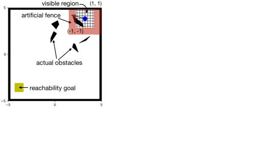
Figure 2: Illustration of dynamic shielding of the robot (blue dot) in an unknown environment. Dynamic shields are computed using ABC, but not over the entire state space, rather over the the tiny visible region of the robot. The corners “$(-1,-1)$” and “$(1,1)$” of the visible region are in the robot’s own reference coordinates.

We need to ensure a safe handover of two dynamically adapted shields at consecutive steps, i.e., every action that a shield allows must guarantee that the new state is in the domain of the shield at the next step. We take a conservative approach. We add artificial fences in the outer periphery of the visible region, to model the uncertainty that awaits in the unobservable parts. This is the worst possible scenario for which the shield must be prepared in the next step. As the robot moves one step after the shield has acted, some states that were previously outside of the visible region may become visible, and some of the states that were previously assumed as unsafe will turn out to actually be safe, thus guaranteeing a safe handover.

We summarize the setting of the dynamic shield synthesis problem to be also used in Section 6. The state space of the robot spans the visible region extended with the artificial fences of a given thickness $\epsilon>0$, i.e., $\mathcal{X}=[-d-\epsilon,d+\epsilon]\times[-d-\epsilon,d+\epsilon]$ with respect to the robot’s own reference coordinate frame, in which the robot’s initial state is always the origin. We use the grid-based abstraction $\widehat{\mathcal{X}}$ of $\mathcal{X}$, and assume that each element of $\widehat{\mathcal{X}}$ is an atomic unsafe state set. This is because at runtime, no matter what obstacles are encountered within the visible region, it can be over-approximated as the union of the right subset of $\widehat{\mathcal{X}}$. In addition, the fence is included in each atomic unsafe set. Therefore, the set of atomic safe sets is $\left\{\mathcal{X}\setminus(\left\{\widehat{x}\right\}\cup\mathit{fence})\mid\widehat{x}\in\widehat{\mathcal{X}}\right\}$ where $\mathit{fence}=\mathcal{X}\setminus[-d,d]\times[-d,d]$.

6 Experiments

The Experimental Setup. The dynamics of the mobile robot is modeled using the discrete-time Dubins vehicle model. The system has three state variables $x$, $y$, and $\theta$, where $x$ and $y$ represent the location in the X-Y coordinate, and $\theta$ represents the heading angle in radians (measured counter-clockwise from the positive X axis); two control input variables $v$ and $a$, representing the forward velocity and the angular velocity of the steering; and three disturbance variables $w^{1},w^{2},w^{3}$, which affect the dynamics in the three individual states. The transitions are:

$$x^{\prime} =x+(v\cos\theta)\tau+w^{1},\qquad y^{\prime} =y+(v\sin\theta)\tau+w^{2},\qquad\theta^{\prime} =\theta+a\tau+w^{3},$$

where the primed variables on the left side represent the states at the next time step, and $\tau$ represents the sampling time. We use the following spaces for the states, control inputs, and disturbance inputs: $x\in[-1,1]$, $y\in[-1,1]$, $\theta\in[-\pi,\pi]$, $v\in\{-0.4,-0.2,\ldots,0.2,0.4\}$, $a\in\{-4,-3.5,\ldots,3.5,4\}$, $w^{1}\in[-0.01,0.01]$, $w^{2}\in[-0.01,0.01]$, and $w^{3}\in[-0.02,0.02]$. Furthermore, we fix $\tau=0.1\,s$, and the thickness of the fence to $\epsilon=0.3$.

The underlying AI controller is generated using reinforcement learning (RL) with reach-avoid objectives. In our experiments, the RL controller is made aware of the entire map, even though the shield’s visibility range is limited to a tiny region ranging $[-1,1]\times[-1,1]$ in its own reference frame.

Table 1: Computation times of the offline phase (atomic shield synthesis) of dynamic shields.

Grid size		Computation time
$\widehat{\mathcal{X}}$	$\widehat{\mathcal{U}}$	Abstraction	Synthesis
$[0.10,0.10,0.30]$	$[0.2,0.5]$	$2\,m\ 12\,s$	$1\,m$
$[0.08,0.08,0.25]$	$[0.2,0.5]$	$4\,m\,40\ s$	$2\,m\ 35\,s$
$[0.06,0.06,0.20]$	$[0.2,0.5]$	$9\,m\ 35\,s$	$9\,m\ 25\,s$

Performance Evaluations. We report the offline and online computation times of our dynamic shields for three different levels of abstraction coarseness used in the ABC algorithms. The abstraction coarseness is measured as the (uniform) grid size used for discretizing the state and input spaces, which are respectively $3$ and $2$-dimensional vectors representing the dimension-wise side lengths of the square-shaped grid elements. All synthesized shields are by-construction safe and minimally permissive, and therefore these aspects are not reported. The code was run on a personal computer powered by Intel Core Ultra 7 255U processor and 32 GB RAM.

We report the offline computation times for the three different abstractions in Table 1. As expected, as the abstraction gets finer (smaller grid sizes), the computation time increases. Nonetheless, all computation finished within reasonable amount of time. In comparison, the pure offline baseline would timeout even for the coarsest abstraction, because with its X-Y state variables’ grid sizes $[0.10,0.10]$, it would create $20\times 20=400$ grid cells in the domain $[-1,1]\times[-1,1]$, and since we choose the number of atomic safety specifications to be equal to the number of grid cells, we would need to solve $2^{400}$ instances of safety controller synthesis problems! Although the pure online baseline takes zero time in the offline phase, it will take more time at the online phase as we discuss next.

For each of the three abstraction classes, we deployed the pure online and dynamic shields alongside a learned controller and tested them on 70 randomly generated reach-avoid control problem instances. In each instance and for each shield, we measured the computation time per step on an average, and report them in Figure 3. We observe that the dynamic shields are almost always faster than the pure online shields, and as the abstraction gets finer, their difference becomes more prominent. With the finest abstraction, the dynamic shield was upto five times faster! Furthermore, any efficiency improvement of the pure online shield would benefit the dynamic shield too, because both rely on the SafetyControl algorithm for their online computation phase.

Figure 3: Average online computation times of the pure online algorithm (the baseline) and our dynamic algorithm. Each point in the scatter plots represents one randomly generated problem instance for the navigation task. The three plots correspond to three different abstraction granularities used in the ABC procedure, with the leftmost plot representing the coarsest (Row 1, Table 1) and the rightmost plot representing the finest (Row 3, Table 1) abstraction sizes.

7 Discussions and Future Work

We propose dynamic shields that can adapt to changing safety specifications at runtime. While the problem can be solved using pure offline or pure online approaches using brute force, our dynamic approach is significantly more efficient and combines both offline and online computations. We presented concrete algorithms using the abstraction-based control framework, and demonstrated the effectiveness of dynamic shields on a robot motion planning problem.

Several future directions exist. Firstly, in our work, we use the atomic safe set as it is given, and we will investigate if this set can be first processed in a way that the online deployment phase of shield computation can be benefited (e.g., by simplifying the nonblockingness process). Secondly, in our simulations of the experiments, sometimes the system would get stuck and would not be able to make progress. This is a known issue in shielding and we will study how to eliminate this by taking inspiration from other works dealing with similar problems [12]. Thirdly, we proposed a conservative but simple approach to the safe handover problem, and more advanced procedures [17] will be incorporated in subsequent versions. Finally, extending to richer settings, like dynamic obstacles and quantitative safety specifications would be a major step.

7.0.1 Acknowledgements

This work was funded in part by the DECO Project (PID2022-138072OB-I00) funded by MCIN/AEI/10.13039/501100011033 and by the ESF+.

References

- [1] Alshiekh, M., Bloem, R., Ehlers, R., Könighofer, B., Niekum, S., Topcu, U.: Safe reinforcement learning via shielding. In: Proceedings of the AAAI conference on artificial intelligence. vol. 32 (2018)
- [2] Anand, A., Nayak, S.P., Schmuck, A.K.: Synthesizing permissive winning strategy templates for parity games. In: International Conference on Computer Aided Verification. pp. 436–458. Springer (2023)
- [3] Bharadwaj, S., Bloem, R., Dimitrova, R., Konighofer, B., Topcu, U.: Synthesis of minimum-cost shields for multi-agent systems. In: 2019 American Control Conference (ACC). pp. 1048–1055. IEEE (2019)
- [4] Bloem, R., Könighofer, B., Könighofer, R., Wang, C.: Shield synthesis: Runtime enforcement for reactive systems. In: International conference on tools and algorithms for the construction and analysis of systems. pp. 533–548. Springer (2015)
- [5] ElSayed-Aly, I., Bharadwaj, S., Amato, C., Ehlers, R., Topcu, U., Feng, L.: Safe multi-agent reinforcement learning via shielding. arXiv preprint arXiv:2101.11196 (2021)
- [6] Feng, Y., Zhu, J., Platzer, A., Laurent, J.: Adaptive shielding via parametric safety proofs. Proceedings of the ACM on Programming Languages 9(OOPSLA1), 816–843 (2025)
- [7] Fridovich-Keil, D., Herbert, S.L., Fisac, J.F., Deglurkar, S., Tomlin, C.J.: Planning, fast and slow: A framework for adaptive real-time safe trajectory planning. In: 2018 IEEE International Conference on Robotics and Automation (ICRA). pp. 387–394. IEEE (2018)
- [8] Henzinger, T.A., Raskin, J.F.: Robust undecidability of timed and hybrid systems. In: International Workshop on Hybrid Systems: Computation and Control. pp. 145–159. Springer (2000)
- [9] Hu, H., Nakamura, K., Fisac, J.F.: Sharp: Shielding-aware robust planning for safe and efficient human-robot interaction. IEEE Robotics and Automation Letters 7(2), 5591–5598 (2022)
- [10] Jansen, N., Könighofer, B., Junges, S., Bloem, R.: Shielded decision-making in mdps. arXiv preprint arXiv:1807.06096 (2018)
- [11] Könighofer, B., Alshiekh, M., Bloem, R., Humphrey, L., Könighofer, R., Topcu, U., Wang, C.: Shield synthesis. Formal Methods in System Design 51, 332–361 (2017)
- [12] Könighofer, B., Rudolf, J., Palmisano, A., Tappler, M., Bloem, R.: Online shielding for reinforcement learning. Innovations in Systems and Software Engineering 19(4), 379–394 (2023)
- [13] Li, S., Bastani, O.: Robust model predictive shielding for safe reinforcement learning with stochastic dynamics. In: 2020 IEEE International Conference on Robotics and Automation (ICRA). pp. 7166–7172. IEEE (2020)
- [14] Majumdar, A., Tedrake, R.: Funnel libraries for real-time robust feedback motion planning. The International Journal of Robotics Research 36(8), 947–982 (2017)
- [15] Majumdar, R., Mallik, K., Rychlicki, M., Schmuck, A.K., Soudjani, S.: A flexible toolchain for symbolic rabin games under fair and stochastic uncertainties. In: International Conference on Computer Aided Verification. pp. 3–15. Springer (2023)
- [16] Majumdar, R., Mallik, K., Schmuck, A.K., Soudjani, S.: Symbolic control for stochastic systems via finite parity games. Nonlinear Analysis: Hybrid Systems 51, 101430 (2024)
- [17] Nayak, S.P., Egidio, L.N., Della Rossa, M., Schmuck, A.K., Jungers, R.M.: Context-triggered abstraction-based control design. IEEE Open Journal of Control Systems 2, 277–296 (2023)
- [18] Nilsson, P., Ozay, N., Liu, J.: Augmented finite transition systems as abstractions for control synthesis. Discrete Event Dynamic Systems 27(2), 301–340 (2017)
- [19] Pola, G., Tabuada, P.: Symbolic models for nonlinear control systems: Alternating approximate bisimulations. SIAM Journal on Control and Optimization 48(2), 719–733 (2009)
- [20] Pranger, S., Könighofer, B., Posch, L., Bloem, R.: Tempest-synthesis tool for reactive systems and shields in probabilistic environments. In: Automated Technology for Verification and Analysis: 19th International Symposium, ATVA 2021, Gold Coast, QLD, Australia, October 18–22, 2021, Proceedings 19. pp. 222–228. Springer (2021)
- [21] Pranger, S., Könighofer, B., Tappler, M., Deixelberger, M., Jansen, N., Bloem, R.: Adaptive shielding under uncertainty. In: 2021 American Control Conference (ACC). pp. 3467–3474. IEEE (2021)
- [22] Quan, L., Zhang, Z., Zhong, X., Xu, C., Gao, F.: Eva-planner: Environmental adaptive quadrotor planning. In: 2021 IEEE International Conference on Robotics and Automation (ICRA). pp. 398–404. IEEE (2021)
- [23] Raeesi, H., Khosravi, A., Sarhadi, P.: Safe reinforcement learning by shielding based reachable zonotopes for autonomous vehicles. International Journal of Engineering 38(1), 21–34 (2025)
- [24] Reissig, G., Weber, A., Rungger, M.: Feedback refinement relations for the synthesis of symbolic controllers. IEEE Transactions on Automatic Control 62(4), 1781–1796 (2016)
- [25] Rungger, M., Zamani, M.: Scots: A tool for the synthesis of symbolic controllers. In: Proceedings of the 19th international conference on hybrid systems: Computation and control. pp. 99–104 (2016)
- [26] Tabuada, P.: An approximate simulation approach to symbolic control. IEEE Transactions on Automatic Control 53(6), 1406–1418 (2008)
- [27] Van Dijk, T., Van De Pol, J.: Sylvan: Multi-core decision diagrams. In: Tools and Algorithms for the Construction and Analysis of Systems: 21st International Conference, TACAS 2015, Held as Part of the European Joint Conferences on Theory and Practice of Software, ETAPS 2015, London, UK, April 11-18, 2015, Proceedings 21. pp. 677–691. Springer (2015)
- [28] Vidal, R., Schaffert, S., Lygeros, J., Sastry, S.: Controlled invariance of discrete time systems. In: International Workshop on Hybrid Systems: Computation and Control. pp. 437–451. Springer (2000)
- [29] Waga, M., Castellano, E., Pruekprasert, S., Klikovits, S., Takisaka, T., Hasuo, I.: Dynamic shielding for reinforcement learning in black-box environments. In: International Symposium on Automated Technology for Verification and Analysis. pp. 25–41. Springer (2022)