ReinFlow: Fine-tuning Flow Matching Policy
with Online Reinforcement Learning

Abstract

We propose ReinFlow, a simple yet effective online reinforcement learning (RL) framework that fine-tunes a family of flow matching policies for continuous robotic control. Derived from rigorous RL theory, ReinFlow injects learnable noise into a flow policy’s deterministic path, converting the flow into a discrete-time Markov Process for exact and straightforward likelihood computation. This conversion facilitates exploration and ensures training stability, enabling ReinFlow to fine-tune diverse flow model variants stably, including Rectified Flow [35] and Shortcut Models [19], particularly at very few or even one denoising step. We benchmark ReinFlow in representative locomotion and manipulation tasks, including long-horizon planning with visual input and sparse reward. The episode reward of Rectified Flow policies obtained an average net growth of 135.36% after fine-tuning in challenging legged locomotion tasks while saving denoising steps and 82.63% of wall time compared to state-of-the-art diffusion RL fine-tuning method DPPO [43]. The success rate of the Shortcut Model policies in state and visual manipulation tasks achieved an average net increase of 40.34% after fine-tuning with ReinFlow at four or even one denoising step, whose performance is comparable to fine-tuned DDIM policies while saving computation time for an average of 23.20%. Project webpage: https://reinflow.github.io/

1 Introduction

Recent years have seen rapid progress in training robotic models via imitation learning. Flow matching models, combining the trifecta of precise modeling, fast inference, and minimal implementation, have emerged as a robust alternative to diffusion policies and a popular choice for robot action generation [8, 6, 58].

However, due to the scarcity of robot data and the embodiment gap, flow policies and many other imitation learning policies are often trained from datasets with mixed quality [13], incurring sub-optimal success rates even after supervised fine-tuning [6]. Although collecting more data may alleviate this issue, recent work [32] suggests that scaling data quantity may not be the panacea because, in a given environment, the success rate quickly plateaus when we solely increase the demonstration number. Worse still, as an imitation learning method, flow policies lack a built-in exploration mechanism, implying that robots trained on imperfect data could struggle to complete challenging tasks where the agent needs to surpass expert demonstrations [5].

Online reinforcement learning (RL) offers a promising solution to these challenges. By learning through trial and error, RL promises to overcome limitations associated with imperfect expert data and even achieve superhuman performance. While recent studies have shown that it is possible to fine-tune diffusion policies via RL [31, 43], training flow models with online RL remains technically challenging.

First, the theory has established that refining a stochastic policy is vital for continuous control problems [50]. However, for conditional flows, whose sample path is governed by a neural ordinary differential equation (ODE), even the log probability-a key factor that measures this stochasticity-could be challenging to obtain and unstable to back-propagate through. This problem is exacerbated when we infer flow policies at very few denoising steps, where the discretization error becomes large at a low inference cost. Second, compared with offline RL methods, online RL fine-tuning requires the policy to balance exploration and exploitation, especially in sparse reward settings [21]. However, how to design a principled exploration mechanism remains elusive for conditional flows with a deterministic path.

This paper addresses these challenges head-on and proposes the first online RL approach to fine-tune a pre-trained flow matching policy. The contributions of this work are summarized as follows:

• Algorithm Design. We propose ReinFlow, the first online RL algorithm to stably fine-tune a family of flow matching policies, especially at very few or even one denoising step. We train a noise injection network to convert flows to a discrete-time Markov Process with Gaussian transition probabilities for exact and tractable likelihood computation. Our design allows the noise net to balance exploration with exploitation automatically; it enjoys lightweight implementation, built-in exploration, and broad applicability to various flow policy variants, including those parameterized with Rectified Flow [35] and Shortcut Models [19].

• Empirical Validation. We perform extensive experiments in representative robot locomotion and manipulation tasks, with the agent receiving state or pixel observations and possibly accepting sparse rewards. Without reward shaping or scaling off-line data, our method, on average, improves the success rate over the pre-trained manipulation policy by 40.34% and increases the reward of locomotion policies by 135.36%. We achieve this improvement with a wall time reduction of 62.82% for all tasks compared to the state-of-the-art RL fine-tuning method for diffusion policies “DPPO” [43].

• Scientific Understanding. We establish a general policy gradient theory for discrete-time Markov process policies that receive partial observations and discounted rewards, which explains our algorithm design for flow matching policies. We also conduct systematic sensitivity analysis on the design choices and key factors that affect the performance of our method, ReinFlow, including the scale of pre-trained data, the number of denoising steps, noise network conditioning, noise level, and the type and intensity of different regularizations.

2 Related Work

In this section, we provide an outline for the relevant works. We defer a detailed introduction for several key baselines to Appendix B.

Online RL for improving diffusion-based policies.

Training diffusion-based policies [3, 12, 40, 44, 51, 54, 57] from demonstrations has recently shown promising results in robot learning tasks. However, their effectiveness is often limited by the quality of demonstrations, especially in settings with mixed or suboptimal data, motivating the need for online fine-tuning.

We can adapt several offline diffusion-based RL methods to online settings. For instance, Diffusion Q Learning (DQL) [55] and Implicit Diffusion Q Learning (IDQL) [24] treat diffusion models as action policies and generally apply Q-learning. DIPO [56] implements a diffusion policy for online RL using a critic to directly update sampled actions via an action gradient. These methods rely on Q-function approximation to guide updates to the diffusion actor, but inaccurate Q estimates can bias updates and destabilize training. Alternatively, methods such as Q Score Matching (QSM) [42], and Diffusion Policy Policy Optimization (DPPO) [43] fine-tune pre-trained diffusion policies with the policy gradient method. While many online RL methods exist for diffusion-based policies, few exist for flow models. The mathematical differences between the two prevent direct transfer of techniques [34], making it challenging to design online RL algorithms for flow policies.

RL for flow matching models.

Flow matching models have demonstrated greater efficiency than diffusion models, offering faster training and sampling and improved generalization [33, 59]. Motivated by their recent success in robot learning [8, 58], image [33, 17] and video generation [28, 53], researchers have explored incorporating these models into RL. Flow Q Learning (FQL) [39] trains a flow policy via offline reinforcement learning (RL) and distills it into a one-step policy for fine-tuning, achieving robust performance in robotic locomotion and manipulation tasks. However, FQL lacks an inherent exploration mechanism for online fine-tuning, which could result in suboptimal, locally convergent solutions [39]. In contrast, our method, ReinFlow, injects bounded and learnable noise into the deterministic trajectory of a flow policy to promote compelling exploration during online fine-tuning. While Flow-GRPO [34] and ORW-CFM-W2 [18] also apply online RL to flow matching, they target computer vision tasks, such as text-to-image generation or image compression, which are distinct from ReinFlow, which is tailored for real-time continuous control in robot learning. Moreover, ReinFlow is a general policy gradient framework that features a small, learnable noise network and performs exact likelihood computation at arbitrarily few denoising steps. However, Flow-GRPO adopts GRPO as a specific policy gradient method and does not learn a noise-injection net; ORW-CFM-W2 is based on reward-weighted regression, which is not a standard policy gradient method.

3 Problem Formulation

Notations

For a positive integer $d$, $\mathbb{R}^{d}$ denotes the $d$-dimensional Euclidean space. For $p\in[1,\infty]$ and $v\in\mathbb{R}^{d}$, $\norm{v}_{p}$ represents the $p$-norm of vector $v$, while $v^{p}$ refers to a vector in $\mathbb{R}^{d}$ created by raising each coordinate of $v$ to the power $p$. $\mathbb{Z}_{\geq 0}$ stands for the set of non-negative integers, and $\mathscr{D}(\mathcal{X})$ denotes the set of probability distributions over the set $\mathcal{X}$. The differential entropy of a continuous random variable $X:\Omega\to\mathcal{X}$ with density $p_{X}(\cdot)$ is given by $\mathbf{h}(X):=-\int_{x\in\mathcal{X}}p_{X}(x)\ln p_{X}(x)\,\mathrm{d}\mu(x)$, where $\mu(\cdot)$ is the Lebesgue measure. We use $\mathcal{N}(\mu,\Sigma)$ to denote a normal distribution with mean $\mu$ and covariance matrix $\Sigma$. With a slight abuse of notation, $\mathbf{h}\circ\mathcal{N}(\mu,\Sigma)$ also represents the differential entropy of a Gaussian random variable.

Robot Learning as a Decision Process

We formulate robot learning as an infinite-horizon Partially Observable Markov Decision Process (POMDP) in continuous state space $\mathcal{S}\in\mathbb{R}^{d_{S}}$, action space $\mathcal{A}\in\mathbb{R}^{d_{A}}$, observation space $\mathcal{O}\in\mathbb{R}^{d_{O}}$, with a discount factor $\gamma\in(0,1)$. The robot plays in an environment with unknown transition kernel $\mathbb{T}_{h,a}(\cdot|s)$ and emission kernel $\mathbb{O}_{h}(\cdot|s)$. The interactions start with an initial state $S_{0}$ drawn from a distribution $\rho\in\mathscr{D}(\mathcal{S})$. In step $h\in\mathbb{Z}_{\geq 0}$, agent observes $o_{h}\sim\mathbb{O}_{h}(\cdot|s_{h})$, takes an action $a_{h}$, before the state $s_{h}$ transitions to $s_{h+1}\sim\mathbb{T}_{h,a_{h}}(\cdot|s_{h})$ with reward $r_{h}$. For simplicity, we study reactive policies, which map the latest observation to an action distribution. The agent aims to maximize the discounted accumulated reward $J(\pi)=\mathbb{E}^{\pi}\left[\sum_{h=1}^{+\infty}\gamma^{h}r_{h}(a_{h},o_{h})\right]$. The Q function $Q_{h}^{\pi}$, value function $V_{h}^{\pi}$ and the advantage function $A_{h}^{\pi}$ are defined as

$$Q_{h}^{\pi}(o_{h},a_{h})= \mathbb{E}^{\pi}\left[\sum_{\tau=h}^{+\infty}\gamma^{\tau-h}r_{\tau}\mid o_{h},a_{h}\right],\ V_{h}^{\pi}(o_{h})=\mathbb{E}^{\pi}[Q_{h}^{\pi}(o_{h},a_{h})|o_{h}],\ A_{h}^{\pi}=Q^{\pi}_{h}-V_{h}^{\pi}$$ (1)

We drop the subscript $h$ for $V^{\pi}_{h}$, $Q^{\pi}_{h}$, and $A^{\pi}_{h}$ when the policy and POMDP are stationary.

Flow Matching Models

Flow matching  [33] transforms random variables from one distribution $p_{0}$ to another $p_{1}$ with flow mappings $\psi:[0,1]\times\mathcal{X}\to\mathcal{X}$, where $X_{t}:=\psi_{t}(X_{0}),t\in[0,1]$. This process is associated with an ODE: $\frac{d}{dt}\psi_{t}(X_{0})=v(t,\psi_{t}(X_{0}))$ where $X_{0}\sim p_{0}$. Rectified flow (ReFlow) [35] is a simple flow model with a straight ODE path $X_{t}=tX_{1}+(1-t)X_{0}$. The velocity field for Rectified Flow satisfies $v(t,X_{t})=\frac{d}{dt}X_{t}=X_{1}-X_{0}$, implying that the training objective for Rectified Flow:

$$\hat{\theta}=\underset{\theta}{\arg\min}\ \mathbb{E}_{X_{0}\sim p_{0},X_{1}\sim p_{1},t\sim\mathrm{Unif}[0,1]}\norm{X_{1}-X_{0}-v_{\theta}\left(t,X_{t}\right)}_{2}^{2}$$ (2)

Practitioners also sample $t$ from beta distribution [7] or logit normal distribution [17]. [19] proposes “Shortcut Models” to further improve the generation quality of Rectified Flow at very few denoising steps by enforcing the velocity generated by two steps to align with that generated by a single step.

During inference, we numerically solve the transport equation by integrating the learned velocity field: $\hat{X}_{1}=X_{0}+\sum_{k=0}^{K-1}v_{\theta}(t_{i},X_{t_{i}})\Delta t_{i}$, where $K$ is the denoising step number, $0=t_{0}<t_{1}<\ldots<t_{K-1}<1=t_{K}$ are the discretized time steps, $\Delta t_{i}=t_{i+1}-t_{i}$ is the step size.

Flow Matching Policy

When we instantiate a flow-matching model in the action generation setting, we obtain a flow-matching policy for robot learning. We denote by $a_{h}^{t}$ the denoised action at time $t$ generated during the $h$-th step of the episode. $\mathcal{X}$ will be the action space $\mathcal{A}$, $p_{0}$ will be the standard normal distribution, and $X_{t}$ corresponds to the robot’s denoised actions. The velocity field $v_{\theta}$ also conditions the observations.

The frequency of inference is a critical factor that affects the dexterity of robot policies, and a faster rollout also reduces the wall time of RL fine-tuning. However, the fewer steps adopted during inference, the higher the discretization error will be, which results in degraded generation quality. We are interested in using RL to improve flow policies with few or even one denoising step so that, after fine-tuning, we get the best of both worlds: fast inference and a high success rate.

4 Algorithm Design

In this section, we elaborate on the design of our algorithm “ReinFlow”.

Algorithm 1 ReinFlow

1:Input pre-trained flow matching policy’s velocity field $v_{\theta}$; denoising step number $K$, discount factor $\gamma$, batch size $B$, discretization scheme $0=t_{0}<t_{1}<\ldots<t_{K}=1\}$ with $\Delta t_{k}:=t_{k+1}-t_{k}$ regularization function ${\mathcal{R}}$ with intensity coefficient $\alpha\in\mathbb{R}$.

2:Initialize noise injection network $\theta^{\prime}$.

3:while not converged do

4:  Restore last iteration’s parameters: $\bar{\theta}_{\mathrm{old}}\leftarrow\mathrm{stop\_grad}([\theta,\theta^{\prime}])$

5:  Reset environment and receive initial observation $o$.

6:  while not $\mathrm{done}$ do$\triangleright$ Rollout policy $\pi$.

7:   Sample $a^{0}\sim\mathcal{N}(0,\mathbb{I}_{d_{A}})$

8:   for denoising step k in $\{0,1,\ldots,K-1\}$ do$\triangleright$ Inject noise and integrate.

9:     $a^{k+1}\leftarrow a^{k}+v_{\theta}(t_{k},a^{k},o)\Delta t_{k}+{{\color[rgb]{0,0,1}\sigma_{\theta^{\prime}}(t_{k},a^{k},o)\epsilon}}$,   $\epsilon\sim\mathcal{N}(0,\mathbb{I}_{d_{A}})$

10:   end for

11:   Record denoised actions $a^{0},a^{1},\ldots,a^{K}$ in a buffer.

12:   Play action $a=a^{K}$, receive reward $r$ and $\mathrm{done}$ flag $d$, update observation $o$.

13:   Store $\{\mathbf{a},o,r,d\}$ to buffer, where $\mathbf{a}:=(a^{0},a^{1},\ldots,a^{K})$

14:  end while

15:  Sample a batch of data $\{\mathbf{a}_{i},o_{i},r_{i},d_{i}\}_{i=1}^{B}$ from buffer. $\triangleright$ Policy Optimization

16:  Compute the policy’s transition probability for each denoising step $k$ and tuple $(\mathbf{a}_{i},o_{i},r_{i},d_{i})$ by Eq. (7):

17:  

$${\color[rgb]{0,0,1}{\ln\pi^{\bar{\theta}}(a_{i}^{k+1}|a_{i}^{k},o_{i})=\ln\mathcal{N}\left(a_{i}^{k+1}|a_{i}^{k}+v_{\theta}\left(t_{k},a_{i}^{k},o_{i}\right)\Delta t_{k}\ ,\ \sigma_{\theta^{\prime}}^{2}\left(t_{k},a_{i}^{k},o_{i}\right)\right)}}$$

18:  Compute the regularization function $\mathcal{R}$ evaluated on each tuple, denoted as $\mathcal{R}(\mathbf{a}_{i},o_{i};\bar{\theta},\bar{\theta}_{\mathrm{old}})$.

19:  Call a policy gradient sub-routine, such as Alg. 2, to jointly optimize $\theta$ and $\theta^{\prime}$ by Eq. (9):

$$\theta,\theta^{\prime}= \ \underset{\theta,\theta^{\prime}}{\mathrm{argmin}}\frac{1}{B}\sum_{i=1}^{B}\left[-A^{\bar{\theta}_{\mathrm{old}}}(o_{i},a_{i}){\color[rgb]{0,0,1}\sum_{k=0}^{K-1}\ln\pi^{\bar{\theta}}(a^{k+1}_{i}|a^{k}_{i},o_{i})}+\alpha\cdot\mathcal{R}(\mathbf{a}_{i},o_{i};\bar{\theta},\bar{\theta}_{\mathrm{old}})\right],\text{where $\bar{\theta}:=[\theta,\theta^{\prime}]$}$$ (3)

20:end while

21:Return fine-tuned flow matching policy’s velocity field $v_{\theta}$.

Algorithm 2 ReinFlow Subroutine for Policy Optimization (PPO implementation)

1:Input clipping range $\epsilon\in(0,1)$, policy parameters at the current iteration $\bar{\theta}:=[\theta,\theta^{\prime}]$ and the last iteration $\bar{\theta}_{\mathrm{old}}$, data $\{\mathbf{a}_{i},o_{i},r_{i},d_{i}\}_{i=1}^{B}$, regularization function values $\{\mathcal{R}(\mathbf{a}_{i},o_{i};{\bar{\theta}},\bar{\theta}_{\mathrm{old}})\}_{i=1}^{B}$, with intensity $\alpha\in\mathbb{R}$.

2:Compute the advantage estimates $\widehat{A}_{i}:=\widehat{A}(o_{i},a_{i}^{K})$ by methods such as GAE [46]

3:Jointly optimize the velocity net $\theta$ and noise net $\theta^{\prime}$ by taking gradient step on the clipped surrogate loss:

$$\nabla_{\bar{\theta}}\ \frac{1}{B}\sum_{i=1}^{B}\left[-\min\left(\frac{\pi_{\bar{\theta}}(\mathbf{a}_{i}|o_{i})}{\pi_{{\bar{\theta}}_{\mathrm{old}}}(\mathbf{a}_{i}|o_{i})}\widehat{A}_{i}\ ,\ \mathrm{clip}\left(\frac{\pi_{\bar{\theta}}(\mathbf{a}_{i}|o_{i})}{\pi_{{\bar{\theta}}_{\mathrm{old}}}(\mathbf{a}_{i}|o_{i})},1-\epsilon,1+\epsilon\right)\widehat{A}_{i}\right)+\alpha\cdot\mathcal{R}(\mathbf{a}_{i},o_{i};{\bar{\theta}},\bar{\theta}_{\mathrm{old}})\right]$$

4:Return updated parameters $\theta,\theta^{\prime}$

4.1 Likelihood Computation over a Short Denoising Trajectory

It is difficult to derive a simple expression for flow matching policy’s log probability at few denoising steps, a vital component for many policy gradient methods [47, 49].

Theory has established an exact expression for the log probability of a continuous-time flow model[11]:

$$\log p_{1}\left(\psi_{1}(x)\right)=\log p_{0}\left(\psi_{0}(x)\right)-\int_{0}^{1}\nabla\cdot v(t,\psi_{t}(x))\ \mathrm{d}t$$ (4)

where $x\sim p_{0}(\cdot)$ is the initial sample. When we discretize the continuous time into sufficiently small time steps, we can adopt the Hutchinson’s trace estimator [25] to approximate Eq. (4):

$$\widehat{\log p_{1}}(x_{1})=\log p_{0}(x_{0})-\sum_{k=0}^{K-1}\tr\left[Z^{\top}\partial_{X}v_{\theta}\left(t_{i},X_{t_{i}}\right)Z\right]\Delta t_{i}$$ (5)

where $Z$ is any zero-mean random vector with identity covariance matrix.

However, it is risky to adopt Eq. (5) directly to compute the likelihood for a flow model with very few denoising steps: Despite the Monte Carlo noise, the time discretization error could be severely high when we reduce the number of steps, which is essential for fast robot action generation.

Although we can alleviate this issue by treating the flow process at inference as a discrete-time Markov process, the intermediate variables follow a deterministic transition, $p(X_{t+\Delta t}=x|X_{t})=\delta\left(x-X_{t}-v_{\theta}(t,X_{t})\Delta t\right)$, making it impossible to compute the probability.

Our approach is different from previous attempts. We inject learnable noise into the flow model’s trajectory, converting flow models into a discrete-time Markov Process. During generation, we sample actions from a normal distribution, whose mean is determined by the velocity field, and the standard deviation is specified by a noise injection network $\theta^{\prime}$. For robot policies, we have

$$a^{0}\sim\mathcal{N}(0,\mathbb{I}_{d_{A}}),\ \ a^{k+1}\sim\mathcal{N}\left(\ \cdot\ |a^{k}+v_{\theta}(t_{i},a^{k},o)\Delta{t_{i}},\ \ \sigma_{\theta^{\prime}}^{2}(t_{i},a^{k},o)\right)$$ (6)

We condition $\theta^{\prime}$ on the generated sigma algebra of $a_{t}$ and $t$ to preserve the Markov property, and consequently, the joint log probability of the noise-injected process admits the following simple and exact expression:

$$\ln\pi(a^{0},\ldots,a^{K}|o;\theta,\theta^{\prime})=\log\mathcal{N}(0,\mathbb{I}_{d_{A}})+\sum_{k=0}^{K-1}\log\ \mathcal{N}\left(a^{k+1}|a_{h}^{k}+v_{\theta}\left(t_{k},a_{h}^{k},o\right)\Delta t_{k}\ ,\ \sigma_{\theta^{\prime}}^{2}\left(t_{k},a^{k},o\right)\right)$$ (7)

where $t_{k}=\frac{k}{K}$ and $\Delta t_{k}=\frac{1}{K}$ under uniform discretization scheme.

Unlike the estimate in Eq. (5), the joint probability expression in Eq. (7) is exact for arbitrarily large step sizes (or equivalently, arbitrarily few denoising steps), which is beneficial for fine-tuning policies with fast inference speed.

4.2 Policy Gradient of a Discrete-time Markov Process

Although Eq. (7) provides the joint probability for the discrete-time Markov process that generates the action via denoising, it does not describe the marginal probability of the last action that the robot will truly execute in the environment. Thankfully, we establish a similar policy gradient theorem for policies parameterized with a discrete-time Markov process, including the noise-injected flow.

Theorem 4.1 (Policy Gradient Theorem for Markov Process Policy).

For a POMDP with a reactive policy $\pi^{\theta}$ described by a discrete-time Markov Process $o_{h}\to a_{h}^{0}\to a_{h}^{1}\to\ldots\to a_{h}^{K}=a_{h}$, the policy gradient is

$$\nabla_{\theta}J(\pi^{\theta})=\mathbb{E}^{\pi^{\theta}}\left[\sum_{h=0}^{+\infty}\gamma^{h}A_{h}^{\pi^{\theta}}(o_{h},a_{h})\nabla_{\theta}\ln\pi^{\theta}(a_{h}^{0},a_{h}^{1},\ldots,a_{h}^{K}|o_{h})\right]$$ (8)

Further assuming that the policy and POMDP are stationary, the policy gradient takes the form of

$$\nabla_{\theta}J(\pi^{\theta}) =\frac{1}{1-\gamma}\mathbb{E}_{o\sim d_{\rho}^{\pi^{\theta}}(\cdot)}\mathbb{E}_{a^{0},a^{1},\ldots,a^{K}\sim\pi^{\theta}(\cdot|o)}\left[Q^{\pi^{\theta}}(o,a)\nabla_{\theta}\sum_{k=0}^{K-1}\ln\pi^{\theta}(a^{k+1}|a^{k},o)\right]$$ (9a)

$$=\frac{1}{1-\gamma}\mathbb{E}_{o\sim d_{\rho}^{\pi^{\theta}}(\cdot)}\mathbb{E}_{a^{0},a^{1},\ldots,a^{K}\sim\pi^{\theta}(\cdot|o)}\left[A^{\pi^{\theta}}(o,a)\nabla_{\theta}\sum_{k=0}^{K-1}\ln\pi^{\theta}(a^{k+1}|a^{k},o)\right]$$ (9b)

where $d_{\rho}^{\pi}$ is the discounted observation visitation frequency, defined as

$$d_{\rho}^{\pi}(o)=(1-\gamma)\mathbb{E}_{s_{1}\sim\rho(\cdot)}\left[\sum_{h=0}^{+\infty}\gamma^{h}\ p(o_{h}=o|s_{1};\pi)\right]$$ (10)

Theorem 4.1 builds on Theorem B.1 in [41] and established results in policy gradient theory [2]. For completeness, we provide the proofs in Appendix A.

Using Eq. (7), we enable the application of various modern deep policy gradient algorithms to optimize a policy parameterized by a discrete-time Markov process, including the noise-injected flows introduced in Section 4.1, which are of particular interest. Specifically, we can optimize the policy using either Eq. (9a) or Eq. (9b). In this work, we implement Eq. (9b) with the clipped surrogate loss [47] due to its stability.

By combining Eq. (7) with Eq. (9), we derive our algorithm, “ReinFlow”, outlined in Alg. 1. We also present one possible policy optimization subroutine in Alg. 2. In Alg. 1, we denote the denoised action sequence $a^{0},\ldots,a^{K}$ as a boldfaced $\mathbf{a}$ and represent the combined parameters of the velocity and noise networks as $\bar{\theta}=[\theta,\theta^{\prime}]$.

We also note that, beyond the implementations in Alg. 1 and Alg. 2, other approaches, such as GRPO [49], can be adopted as a subroutine to implement Eq. (9a). Alternatively, we can optimize Eq. (9b) by replacing Eq. (3) with:

$$\theta,\theta^{\prime}= \ \underset{\theta,\theta^{\prime}}{\mathrm{argmin}}\frac{1}{B}\sum_{i=1}^{B}\left[-Q^{\bar{\theta}_{\mathrm{old}}}(o_{i},a_{i}){\sum_{k=0}^{K-1}\ln\pi^{\bar{\theta}}(a^{k+1}_{i}|a^{k}_{i},o_{i})}+\alpha\cdot\mathcal{R}(\mathbf{a}_{i},o_{i};{\bar{\theta}})\right],\text{where $\bar{\theta}:=[\theta,\theta^{\prime}]$}$$ (11)

and employ off-policy methods, such as SAC [23], to update the policy.

In practice, we adopt “action chunking” during policy execution [30], in which the policy outputs multiple actions in a batch given an observation. We explain how action chunking affects likelihood computation in Appendix A.2.

4.3 Noise Injection Network

We can choose to condition the noise injection network $\sigma$ on $o$, $(o,t)$, or even force it to output fixed constants. We provide a comparative study in Section 6 to analyze how $\sigma$’s inputs affect ReinFlow’s performance.

When the noise injection network is learnable, it uses features from the pre-trained flow policy to save parameters and ensure consistency. It outputs a bounded vector indicating the standard deviation of the Gaussian noise added to each coordinate of the action. We determine the bounds on the noise by a set of key hyperparameters that vary according to the mechanical structural constraints of each joint. We study the effect of the bounds on the noise in Section 5. We also demonstrate in Table 2 that our noise injection network utilizes only a fraction of the parameters of the pre-trained policy.

During fine-tuning, the noise injection network $\theta^{\prime}$ is trained with the velocity network $\theta$ to add diversity to the sample path for better exploration. The loss function for $\theta^{\prime}$ is the policy gradient loss (Eq. (9)), the same for the velocity net. After fine-tuning, we discard the noise net $\theta^{\prime}$ and recover the flow matching policy, which is still composed of deterministic maps.

4.4 Regularization

ReinFlow also supports various ways to regularize the fine-tuned policy.

$W_{2}$ regularization.

One approach is to adopt Wasserstein regularization [29, 39], which constrains the Wasserstein-2 distance from the fine-tuned policy to the pre-trained policy. Studies show that $W_{2}$ regularization could improve training stability for generative models [4, 29]. In practice, we minimize a tractable upper bound on this distance to enforce such constraint:

$$\mathcal{R}_{\text{W}_{2}}(\theta,\theta_{\mathrm{old}}) =\mathbb{E}_{o}\mathbb{E}_{a\sim\pi_{\theta}(\cdot|o),a_{\mathrm{old}}\sim\pi_{\theta_{\mathrm{old}}}(\cdot|o)}\left[\tfrac{1}{2}\norm{a-a_{\mathrm{old}}}_{2}^{2}\right]$$ (12)

$$\geq\mathbb{E}_{o}\left[\inf_{\lambda\in\Lambda}\mathbb{E}_{x,y\sim\lambda_{o}}\left[\tfrac{1}{2}\norm{|x-y}_{2}^{2}\right]\right]=\mathbb{E}_{o}\left[W_{2}^{2}(\pi_{\theta_{\mathrm{old}}}(\cdot|o),\pi_{\theta}(\cdot|o))\right]$$

In Eq. (12), $\Lambda_{o}$ indicates the set of distributions over $\mathcal{A}^{2}$ whose marginals are $\pi_{\theta_{\mathrm{old}}}(\cdot|o)$ and $\pi_{\theta}(\cdot|o)$. To implement Eq. (12), we replace the expectations with the sample mean over a batch of data. Inspired by [39], we integrate $a$ and $a_{\mathrm{old}}$ from the same starting noise $a_{0}\sim\mathcal{N}(0,\mathbb{I}_{d_{A}})$, to control the stochasticity of the initial denoise action. We also note that when computing $\mathcal{R}_{W_{2}}$, we do not inject noise when sampling $a$ from $\pi_{\theta}$.

Entropy regularization.

Another technique is entropy regularization, which theory has shown accelerates convergence [1, 10] and encourages exploration [23] for simple policy classes. For a flow matching policy parameterized with a discrete-time Markov process, we adopt the negative per-symbol entropy rate (or block entropy) [48] as the entropy regularizer. For a stationary POMDP and policy, we define the regularizer as follows:

$$\mathcal{R}_{\mathbf{h}}(\bar{\theta})= -\frac{1}{K+1}\mathbb{E}\ \left[\mathbf{h}(a^{0},a^{1},\ldots,a^{K}|o,\bar{\theta})\right]$$

$$= -\frac{1}{K+1}\mathbb{E}\ \left[\mathbf{h}\circ\mathcal{N}(0,\mathbb{I}_{d_{A}})+\sum_{k=0}^{K-1}\mathbf{h}\circ\mathcal{N}\left(a^{k}+v_{\theta}(t_{k},a^{k},o)\Delta t_{k}\ ,\sigma_{\theta^{\prime}}^{2}(t_{k},a^{k},o)\right)\right]$$

Here, the last step is due to the definition of the noise-injected flow process in Eq. (6). $\mathbf{h}$ is the differential entropy operator [14], of which normal distributions possess a simple closed-form expression (see, e.g. Lemma 7.4 in [15]). According to [48], the per-symbol entropy measures the Shannon entropy of a finite symbol sequence with long-range correlations. By minimizing $\mathcal{R}_{\mathbf{h}}$, we promote the agent to seek more diverse actions, enhancing exploration.

We carry out experiments in Section 5 to compare the effects of different regularizations on the performance of ReinFlow. By default, we adopt entropy regularization in Algorithm 1 for state-input tasks and do not adopt regularization for visual manipulation tasks.

5 Experiments

We run simulated robot learning experiments to test the effectiveness and flexibility of our method, ReinFlow. We aim to adopt ReinFlow to significantly enhance the success rate of pre-trained flow matching policies trained on mediocre expert data. We also managed to fine-tune at very few or even one denoising step for Rectified Flow (indicated by “ReinFlow-R”) and Shortcut Models (indicated by “ReinFlow-S”), where fine-tuning the two types of pre-trained models shares the same training hyperparameters.

We adopt a PPO-based implementation of our algorithm due to its stability. While alternative implementations may offer higher sample efficiency, we prioritize wall time efficiency in simulated environments over sample cost. Exploring more sample-efficient RL algorithms for ReinFlow, especially in real-world scenarios where data collection is expensive, is an interesting direction for future work.

We compare ReinFlow against various RL methods for fine-tuning diffusion and flow-based policies, particularly DPPO and FQL. DPPO is a strong online RL algorithm for diffusion policies, developed under a bi-level MDP formulation [43]. FQL represents state-of-the-art offline RL for flow-matching policies and applies to offline-to-online fine-tuning. Comparisons to other baselines are provided in Appendix E.

5.1 Environment Setup and Data Curation

We compare the algorithms in locomotion tasks and four manipulation tasks. In locomotion tasks, the agent receives state input and dense reward, and it resembles how we train legged robots via sim2real RL in modern applications [45]. We also consider more challenging and realistic manipulation tasks, where agents receive pixel and/or state inputs with sparse rewards.

OpenAI Gym [9].

We fine-tuned flow matching policies with ReinFlow in “Hopper-v2”, “Walker2d-v2”, “Ant-v2” and “Humanoid-v3” where these tasks are listed in ascending difficulty. “Ant-v2” and “Humanoid-v3” environments involve high-dimensional state inputs and challenge continuous control problems. The expert data are demonstrations collected from the D4RL dataset [20]   at medium or medium-expert level.

Franka Kitchen [22].

In Franka Kitchen, a 9-DoF Franka robot learns long-horizon multitask planning by sequentially completing four state-based manipulation tasks. We pre-train the models with human-teleoperated data with complete, mixed, or partial demonstrations of the four tasks.

Robomimic [37].

We train agents in visual manipulation tasks in Robomimic, including a simple pick-and-place task “PickPlaceCan” (Can), assembly task “NutAssemblySquare”(Square), and bi-manual manipulation task “TwoArmTransport”(Transport). Data are collected via human teleportation. The Robomimic datasets are further processed like DPPO [43], which contains data of lower quantity and/or quality than proficient human demonstrations.

5.2 Performance Evaluation

ReinFlow demonstrates strong training stability with a significant reward or success rate net increase in all tasks. In Gym and Franka Kitchen benchmarks, it achieves the best overall efficiency and performance improvement.

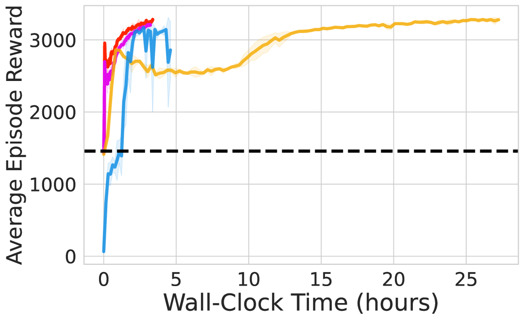
(a) Hopper-v2

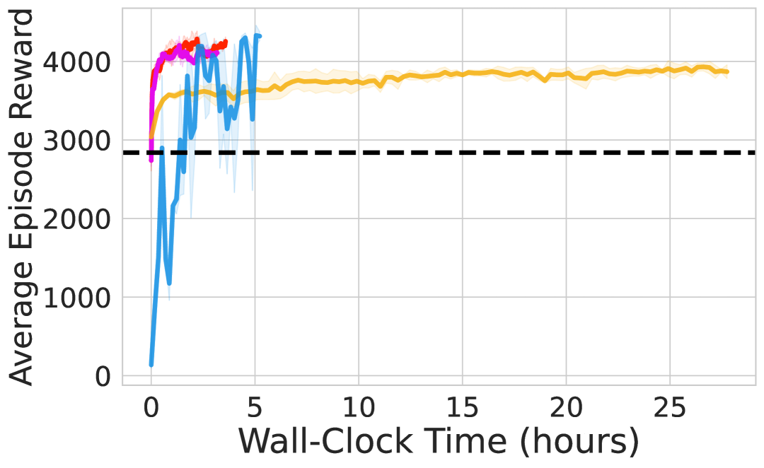
(b) Walker-v2

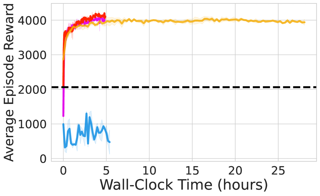
(c) Ant-v2

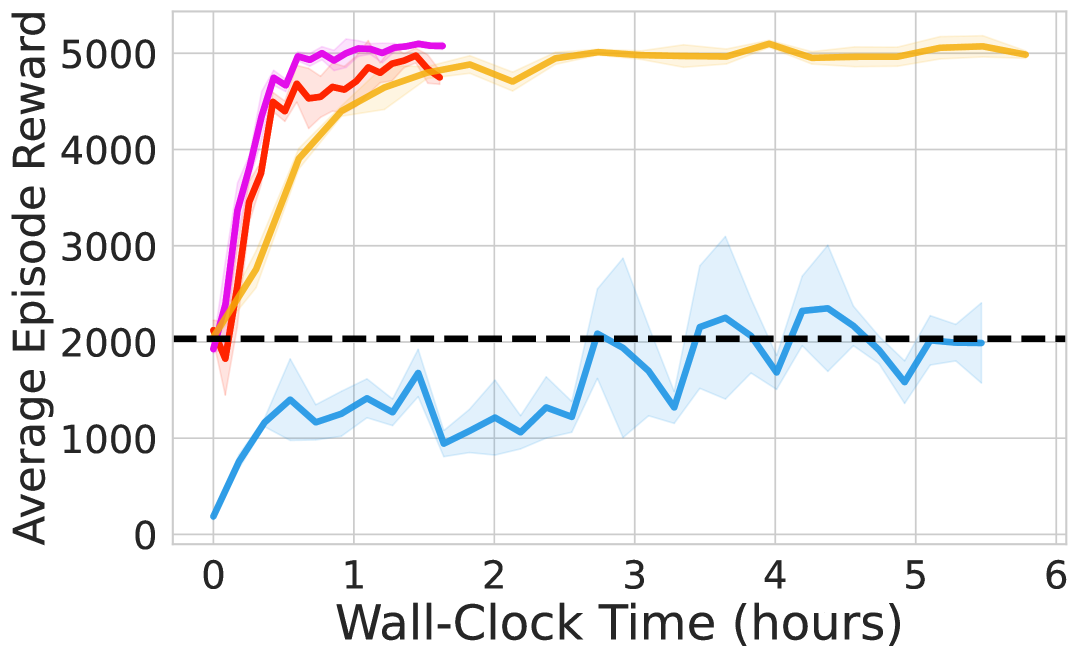
(d) Humanoid-v3

Figure 1: Wall time efficiency results of state-based locomotion tasks in OpenAI Gym. Dashed lines indicate the behavior cloning level.

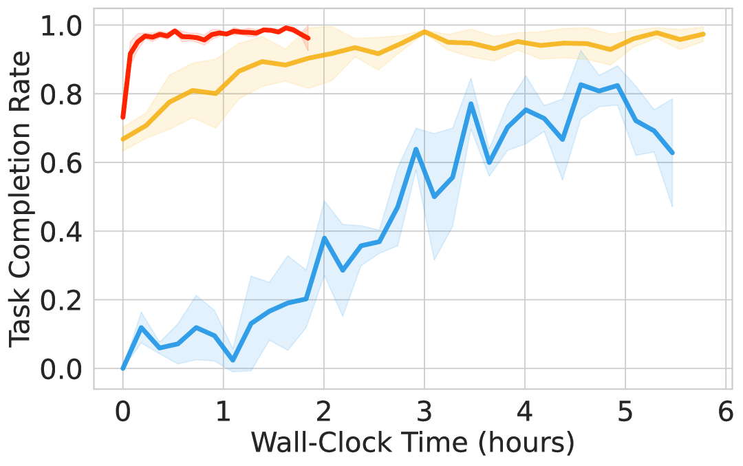
(a) Kitchen-complete

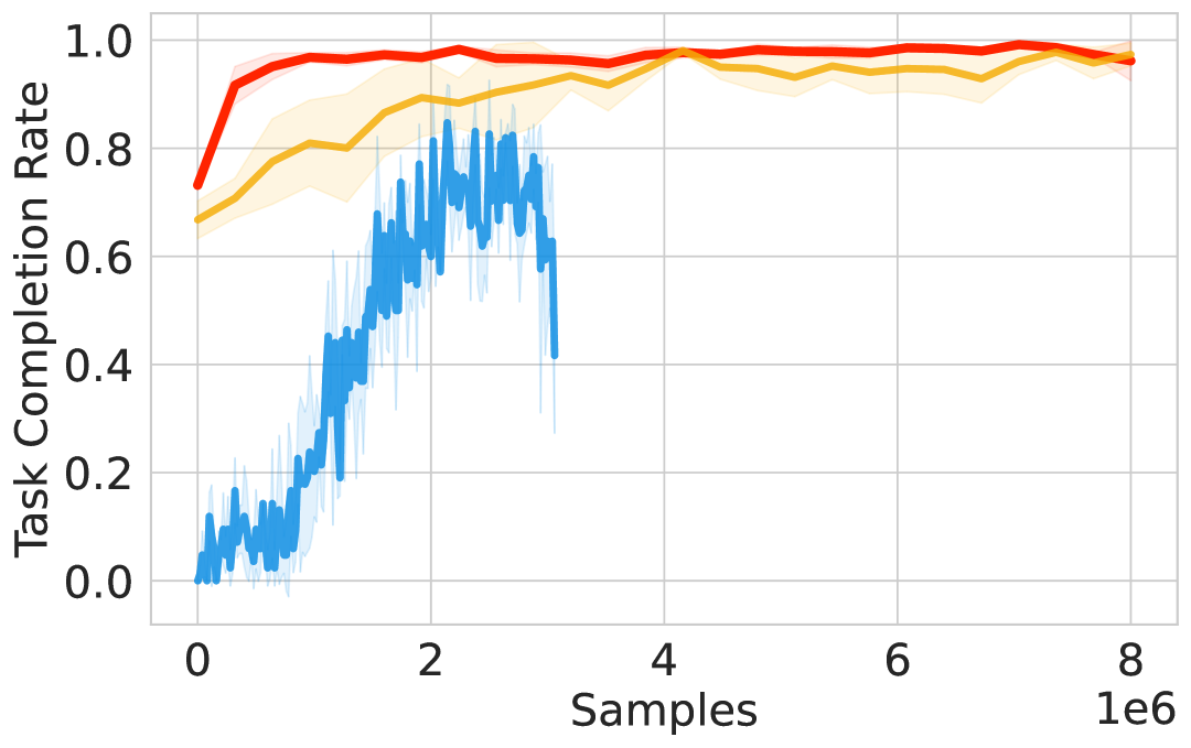
(b) Kitchen-complete

(c) Kitchen-mixed

(d) Kitchen-partial

Figure 2: Task completion rates of state-input manipulation tasks in Franka Kitchen. (a) and (b) show the completion rates against the wall time and sample cost. We only show the sample cost plots for agents trained on mixed and partial datasets for brevity.

Across three Robomimic visual manipulation tasks, ReinFlow-S and ReinFlow-R improve the success rate of the pre-trained policy by an average of 45.77%. ReinFlow achieves success rates comparable to DPPO, requiring significantly fewer fine-tuning steps and less wall-clock time. Notably, it uses fewer denoising steps: just one in can and square, and a four-step flow in transport, compared to the five-step DDIM used by DPPO.

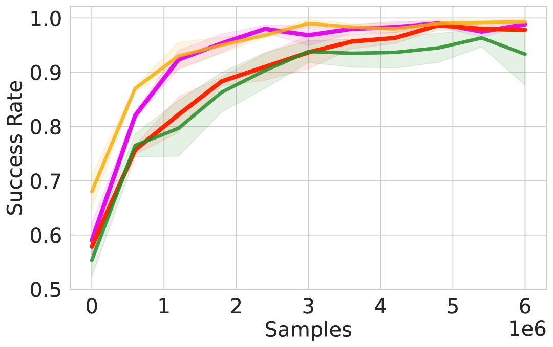
(a) Can

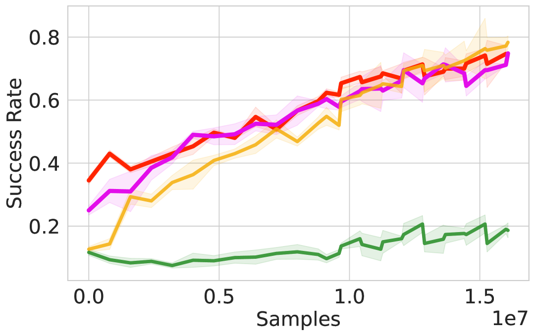
(b) Square

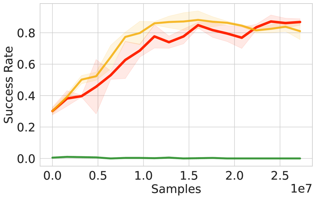
(c) Transport

Figure 3: Success rates in visual manipulation tasks in Robomimic.

6 The Design Choice and Key Factors Affecting ReinFlow

This section analyzes how the pre-trained model and denoising steps affect our algorithm. We also study the effects of the noise level, the type, and the intensity of regularization.

Scaling.

We fine-tune flow matching policies trained on datasets with different numbers of episodes and test the performance of pre-trained and fine-tuned models at different denoising steps. Fig 4(a) reveals that scaling inference steps and/or pre-training data quantity does not consistently improve the reward, which is consistent with the findings in  [32]. However, ReinFlow consistently improves the success rate or reward over the pre-trained policies regardless of the pre-training scale.

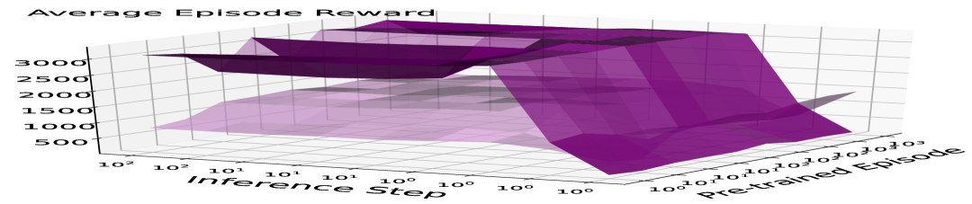
(a) ReFlow Policy in Hopper-v2

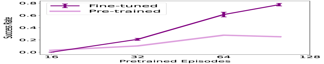
(b) Shortcut Policy in Square

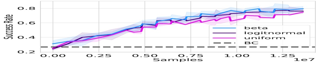
(c) ReFlow Policy in Square

Figure 4: RL provides another way of scaling apart from increasing pre-training data and inference consumption, which has a plateauing effect. The improvement is invariant of flow policy’s time distribution and is achievable at four steps in Hopper (Fig. 4(a)) and one step in Square (Figs. 4(b),  4(c)).

Flow Matching’s Time Distribution.

The effectiveness of ReinFlow is not affected by altering the time sampling distribution of the pre-trained flow matching policy. However, beta distribution is slightly stronger when fine-tuning at one denoising step, as in the case in Fig. 4(c).

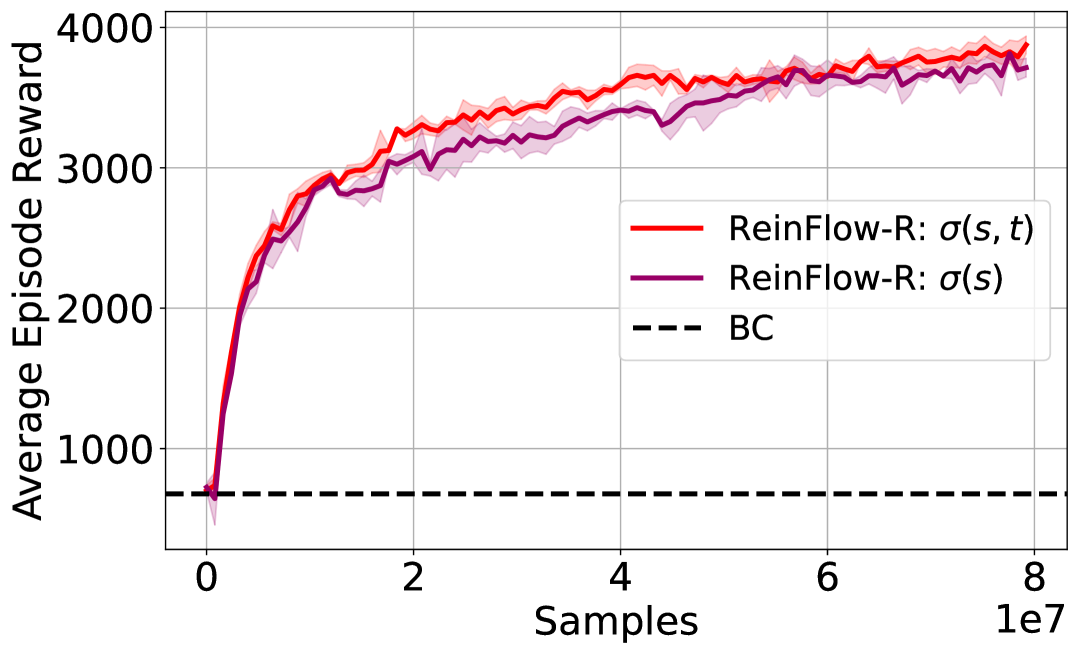
(a) Noise Input’s Effect in Ant-v0

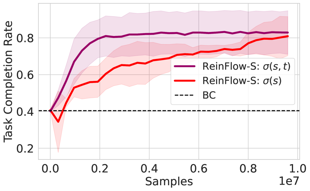
(b) Noise Condition’s Effect in Kitchen-partial

Figure 5: Conditioning on state and time yields a higher success rate than only conditioning on states.

Noise Network Inputs.

The inputs of the noise injection network affect the performance of fine-tuned flow policies. As shown in Fig. 5, conditioning on both observations and the time often yields a higher success rate, as this approach allows the noise network to learn how to create more diverse actions by altering the noise intensity at different denoising steps.

Noise Level and Exploration.

We find that the magnitude of the injected noise is the most significant factor affecting ReinFlow’s performance. In Fig. 6(a), we add constant noise in ’Ant-v0’ with different standard deviation levels. When the noise is minimal ($\mathrm{std}=0.01$), the policy’s reward remains around the pre-trained baseline, showing limited exploration. After enlarging the noise to a certain threshold, we find that the agent quickly explores new policies that are three times stronger than the base policy, after which ReinFlow becomes less sensitive to changes in noise level. We also discover that tuning down the noise is beneficial for visuomotor policies, complex tasks, long denoising chains, and policies with poor pre-training performance.

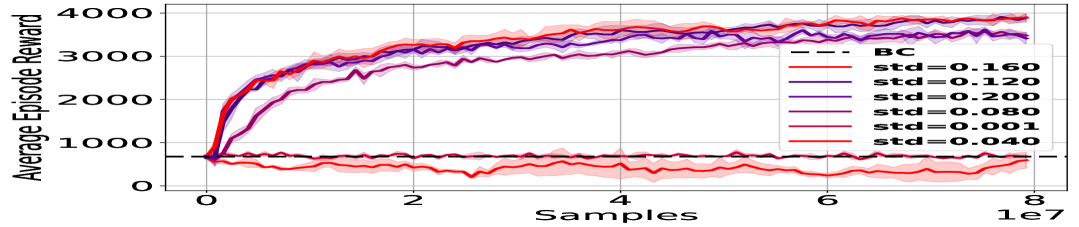
(a) Noise Level Affects Exploration in Ant-v0

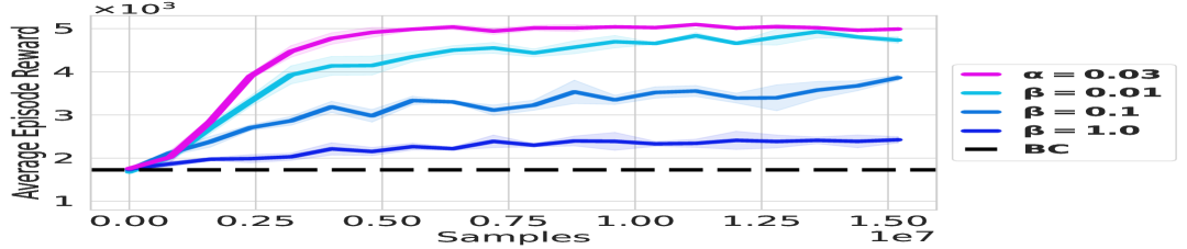
(b) Regularization Affects ReinFlow in Humanoid-v3

Figure 6: Noise level and regularization’s Effect. Fig. 6(a) demonstrates constant noise with different standard deviation affects ReinFlow’s exploration. In Fig. 6(b), we show how entropy regularization with coefficient $\alpha$ and $W_{2}$ regularization with different coefficients $\beta$ influences ReinFlow.

Regularization and Exploration.

ReinFlow admits various regularizations, and we find that it is generally unnecessary to constrain the policy with a Wasserstein-2 regularizer while adding entropy regularization, which is beneficial in locomotion tasks. In Fig. 6(b), we train ReinFlow in a “Humanoid-v3” environment. By gradually tuning down the $W_{2}$ regularization coefficient $\beta$, the fine-tuned policy leaves the behavior cloning (BC) baseline and discovers significantly more robust actions, approaching the curve trained with entropy regularization of intensity $\alpha=0.03$. This finding also partially explains why the offline RL method FQL, which adopts $W_{2}$ distillation loss to restrict online exploration, performs worse than our pure online RL method ReinFlow.

7 Conclusion and Future Work

This work introduces ReinFlow, the first online reinforcement learning framework that stably fine-tunes a family of flow matching policies for continuous robotic control at arbitrarily few denoising steps. In state-input locomotion and visual manipulation tasks, ReinFlow surpasses existing methods that fine-tune diffusion or flow models using RL while reducing wall-clock time by 62.82% in all tasks compared to the state-of-the-art diffusion RL fine-tuning algorithm DPPO. We also provide rigorous theoretical support for our algorithm design and conduct a comprehensive sensitivity analysis to identify the key factors affecting ReinFlow’s performance.

It is a promising future direction to implement ReinFlow with other policy gradient methods, and deploy the fine-tuned policy in the real world. We leave these to future work.

Acknowledgements

This work was supported by National Natural Science Foundation of China (No.62406159, 62325405), Postdoctoral Fellowship Program of CPSF under Grant Number (GZC20240830, 2024M761676), China Postdoctoral Science Special Foundation 2024T170496. The authors are grateful to Shu’ang Yu for reviewing the earlier versions of the paper. We also thank Feng Gao, Cheng Yin, and Ningyuan Yang for many fruitful discussions and comments.

We provide a schematic in Fig 7 to illustrate the procedure of fine-tuning a flow matching policy with ReinFlow.

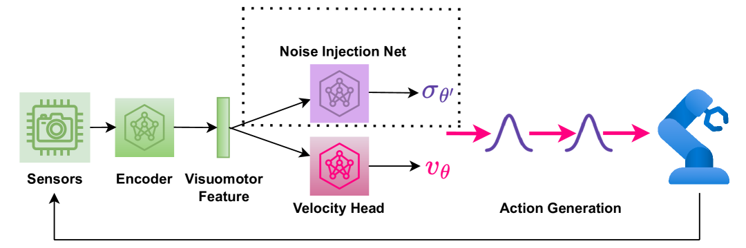
Figure 7: Fine-tuning a flow matching policy with online RL algorithm ReinFlow (Alg. 1). Through interactions with the environment, the robot collects visual and proprioceptive signals, from which a pre-trained policy extracts features and outputs the velocity field of the following action, $v_{\theta}$. A noise injection network $\sigma_{\theta^{\prime}}$ shares the extracted features with $v_{\theta}$ and outputs a Gaussian noise that smoothens the flow’s deterministic ODE path, converting flows to a discrete-time Markov process with Gaussian transition probabilities. The noise injection yields an exact and straightforward likelihood expression at any denoising steps, which is friendly for policy gradient optimization. The noise injection net $\sigma_{\theta^{\prime}}$, surrounded by the dot lines, co-trained with $v_{\theta}$ but will be discarded after fine-tuning. The size of $\sigma_{\theta^{\prime}}$ is only a fraction of the pre-trained flow policy.

We outline our findings on a webpage: https://reinflow.github.io/. In what follows, we provide the theoretical background of our algorithm, report the findings omitted by the main text, and elaborate on the implementation details required to reproduce our experimental results.

Appendix A Theoretical Support

A.1 Proof of Theorem 4.1

In this section, we prove Theorem 4.1, the policy gradient theorem for discrete-time Markov process policies.

For notation simplicity, we only consider an infinite-horizon POMDP with a reactive policy. We obtain the result for the finite-horizon setting by imposing $r_{h}=0$ for $h$ larger than the finite horizon $H$. For the reader’s convenience, we recall several fundamental definitions of RL. The objective function for RL is given by $J(\pi)=\mathbb{E}^{\pi}\left[\sum_{h=0}^{+\infty}\gamma^{h}r_{h}(o_{h},a_{h})\right]$, The value function, Q function, and the advantage functions are defined as

$$V^{\pi}_{h}(o_{h})= \mathbb{E}^{\pi}\left[\sum_{\tau=h}^{+\infty}\gamma^{\tau-h}r_{\tau}(a_{\tau},o_{\tau})\mid o_{h}\right]$$ (13)

$$Q^{\pi}_{h}(o_{h},a_{h})= \mathbb{E}^{\pi}\left[\sum_{\tau=h}^{+\infty}\gamma^{\tau-h}r_{\tau}(a_{\tau},o_{\tau})\mid o_{h},a_{h}\right]\quad A_{h}^{\pi}(o_{h},a_{h})=Q^{\pi}_{h}(o_{h},a_{h})-V^{\pi}(o_{h})$$

We first show that we can express the policy gradient for POMDP in terms of the advantage function and the action log probability’s gradient:

$$\nabla_{\theta}J(\pi^{\theta})=\mathbb{E}^{\pi^{\theta}}\left[\sum_{\tau=0}^{+\infty}\gamma^{\tau}A_{\tau}^{\pi^{\theta}}(o_{\tau},a_{\tau})\nabla_{\theta}\ln\pi_{\theta}(a_{\tau}|o_{\tau})\right]$$ (14)

Remark A.1.

In Eq. (14), we use $\theta$ to indicate general policy parameters. $\theta$ should be understood as $\bar{\theta}=[\theta,\theta^{\prime}]$, that is, the combination of the velocity and noise nets when we instantiate the policy as a noise-injected flow matching policy.

Proof.

$$\nabla_{\theta}J(\pi^{\theta})= \sum_{h=0}^{+\infty}\gamma^{h}\int_{\mathcal{O\times A}^{h}}r_{h}(o_{h},a_{h})\cdot\nabla_{\theta}p(o_{1:h},a_{1:h}|\pi^{\theta})$$

$$= \sum_{h=0}^{+\infty}\gamma^{h}\int_{\mathcal{O\times A}^{h}}r_{h}(o_{h},a_{h})\cdot\nabla_{\theta}\exp\ln p(o_{1:h},a_{1:h}|\pi^{\theta})$$

$$= \sum_{h=0}^{+\infty}\gamma^{h}\int_{\mathcal{O\times A}^{h}}r_{h}(o_{h},a_{h})\cdot p(o_{1:h},a_{1:h}|\pi^{\theta})\nabla_{\theta}\ln p(o_{1:h},a_{1:h}|\pi^{\theta})$$

$$\overset{(i)}{=} \sum_{h=0}^{+\infty}\gamma^{h}\int_{\mathcal{O\times A}^{h}}r_{h}(o_{h},a_{h})\cdot p(o_{1:h},a_{1:h}|\pi^{\theta})\sum_{\tau=1}^{h}\nabla_{\theta}\ln\pi_{\theta}(a_{\tau}|o_{\tau})$$

$$= \mathbb{E}^{\pi^{\theta}}\left[\sum_{h=0}^{+\infty}\gamma^{h}r_{h}(o_{h},a_{h})\sum_{\tau=1}^{h}\nabla_{\theta}\ln\pi_{\theta}(a_{\tau}|o_{\tau})\right]$$

$$= \mathbb{E}^{\pi^{\theta}}\left[\sum_{\tau=0}^{+\infty}\sum_{h=\tau}^{+\infty}\gamma^{h}r_{h}(o_{h},a_{h})\nabla_{\theta}\ln\pi_{\theta}(a_{\tau}|o_{\tau})\right]\quad\text{// Change summation order}$$

$$= \mathbb{E}^{\pi^{\theta}}\left[\sum_{\tau=0}^{+\infty}\gamma^{\tau}\nabla_{\theta}\ln\pi_{\theta}(a_{\tau}|o_{\tau})\sum_{h=\tau}^{+\infty}\gamma^{h-\tau}r_{h}(o_{h},a_{h})\right]$$

$$= \mathbb{E}^{\pi^{\theta}}\left[\sum_{\tau=0}^{+\infty}\gamma^{\tau}\nabla_{\theta}\ln\pi_{\theta}(a_{\tau}|o_{\tau})\mathbb{E}\left[\sum_{h=\tau}^{+\infty}\gamma^{h-\tau}r_{h}(o_{h},a_{h})\mid a_{\tau},o_{\tau}\right]\right]$$

$$= \mathbb{E}^{\pi^{\theta}}\left[\sum_{\tau=0}^{+\infty}\gamma^{\tau}Q_{\tau}^{\pi^{\theta}}(o_{\tau},a_{\tau})\nabla_{\theta}\ln\pi_{\theta}(a_{\tau}|o_{\tau})\right]\quad\text{// Definition in Eq.~\eqref{eq:q_value_def_reiterate}}$$

$$= \mathbb{E}^{\pi^{\theta}}\left[\sum_{\tau=0}^{+\infty}\gamma^{\tau}Q_{\tau}^{\pi^{\theta}}(o_{\tau},a_{\tau})\nabla_{\theta}\ln\pi_{\theta}(a_{\tau}|o_{\tau})\right]-\underbrace{\sum_{\tau=0}^{+\infty}\frac{\gamma^{\tau}V^{\pi^{\theta}}}{\pi_{\theta}(a_{\tau}|o_{\tau})}\nabla_{\theta}\int_{\mathcal{A}}\mathrm{d}a_{\tau}\pi_{\theta}(a_{\tau}|o_{\tau})}_{=0}$$

$$= \mathbb{E}^{\pi^{\theta}}\left[\sum_{\tau=0}^{+\infty}\gamma^{\tau}A_{\tau}^{\pi^{\theta}}(o_{\tau},a_{\tau})\nabla_{\theta}\ln\pi_{\theta}(a_{\tau}|o_{\tau})\right]\quad\text{// Definition in Eq.~\eqref{eq:q_value_def_reiterate}}$$

where (i) is due to the Markov property:

$$\nabla_{\theta}\ln p(o_{1:t},a_{1:t}|\pi^{\theta})$$ (15)

$$= \nabla_{\theta}\left(\ln\left(\rho(s_{1})\cdot\mathbb{O}_{1}(o_{1}|s_{1})\cdot\pi_{\theta}(a_{1}|o_{1})\cdot\mathbb{T}_{h}(s_{2}|s_{1},a_{1})\cdot\ldots\cdot\mathbb{O}_{h}(o_{h}|a_{h})\cdot\pi_{\theta}(a_{h}|o_{h})\right)\right)$$

$$= \nabla_{\theta}\ln\pi_{\theta}(a_{1}|o_{1})+\nabla_{\theta}\ln\pi_{\theta}(a_{2}|o_{2})+\ldots+\nabla_{\theta}\ln\pi_{\theta}(a_{t}|o_{t})$$

∎

Next, we extend Theorem 1 in [41] and study the case when the action is generated via a Markov Process. The action probability is expressed by

$$\pi_{\theta}(a_{h}|o_{h})= \int_{\mathcal{A}^{K}}{\mathrm{d}a}_{h}^{0}{\mathrm{d}a}_{h}^{1}\ldots{\mathrm{d}a}_{h}^{K-1}\ \pi_{\theta}(a_{h}^{0},a_{h}^{1},\ldots,a_{h}^{K}|o_{h})$$ (16)

$$= \int_{\mathcal{A}^{K}}{\mathrm{d}a}_{h}^{0}{\mathrm{d}a}_{h}^{1}\ldots{\mathrm{d}a}_{h}^{K-1}\ \pi_{\theta}(a_{h}^{0}|o_{h})\cdot\prod_{k=0}^{K-1}\pi_{\theta}(a_{h}^{k+1}|a_{h}^{k},o_{h})$$

where we write $a_{h}=a_{h}^{K}$. Bringing Eq. (16) to Eq. (14), we obtain

$$\nabla_{\theta}J(\pi^{\theta})$$ (17)

$$= \mathbb{E}^{\pi^{\theta}}\left[\sum_{\tau=0}^{+\infty}\gamma^{\tau}A_{\tau}^{\pi^{\theta}}(o_{\tau},a_{\tau})\nabla_{\theta}\ln\pi_{\theta}(a_{\tau}|o_{\tau})\right]$$

$$= \sum_{\tau=0}^{+\infty}\gamma^{\tau}\int_{\mathcal{A}}\mathrm{d}a_{\tau}\cancel{\pi_{\theta}(a_{\tau}|o_{\tau})}A_{\tau}^{\pi^{\theta}}(o_{\tau},a_{\tau})\frac{1}{\cancel{\pi_{\theta}(a_{\tau}|o_{\tau})}}\nabla_{\theta}\pi_{\theta}(a_{\tau}|o_{\tau})$$

$$= \sum_{\tau=0}^{+\infty}\gamma^{\tau}\int_{\mathcal{A}}\mathrm{d}a_{\tau}^{K}A_{\tau}^{\pi^{\theta}}(o_{\tau},a_{\tau})\cdot\left[\int_{\mathcal{A}^{K}}\mathrm{d}a_{\tau}^{0}\mathrm{d}a_{\tau}^{1}\ldots\mathrm{d}a_{\tau}^{K-1}\ \nabla_{\theta}\left(\pi_{\theta}(a_{\tau}^{0}|o_{\tau})\cdot\prod_{t=0}^{K-1}\pi_{\theta}(a_{\tau}^{t+1}|a_{\tau}^{t},o_{\tau})\right)\right]$$

$$= \sum_{\tau=0}^{+\infty}\gamma^{\tau}\int_{\mathcal{A}^{K+1}}\mathrm{d}a_{\tau}^{0}\cdots\mathrm{d}a_{\tau}^{K}\cdot A_{\tau}^{\pi^{\theta}}(o_{\tau},a_{\tau})\cdot\left[\nabla_{\theta}\exp\ln\pi_{\theta}(a_{\tau}^{0},a_{\tau}^{1},\ldots,a_{\tau}^{K}|o_{\tau})\right]$$

$$= \sum_{\tau=0}^{+\infty}\gamma^{\tau}\int_{\mathcal{A}^{K+1}}\mathrm{d}a_{\tau}^{0}\cdots\mathrm{d}a_{\tau}^{K}\cdot A_{\tau}^{\pi^{\theta}}(o_{\tau},a_{\tau})\cdot\left[\pi_{\theta}(a_{\tau}^{0},a_{\tau}^{1},\ldots,a_{\tau}^{K}|o_{\tau})\cdot\nabla_{\theta}\ln\pi_{\theta}(a_{\tau}^{0},a_{\tau}^{1},\ldots,a_{\tau}^{K}|o_{\tau})\right]$$

$$= \mathbb{E}^{\pi^{\theta}}\left[\sum_{\tau=0}^{+\infty}\gamma^{\tau}A_{\tau}^{\pi^{\theta}}(o_{\tau},a_{\tau})\nabla_{\theta}\ln\pi_{\theta}(a_{\tau}^{0},a_{\tau}^{1},\ldots,a_{\tau}^{K}|o_{\tau})\right]$$

$$= \mathbb{E}^{\pi^{\theta}}\left[\sum_{\tau=0}^{+\infty}\gamma^{\tau}A_{\tau}^{\pi^{\theta}}(o_{\tau},a_{\tau})\nabla_{\theta}\sum_{k=0}^{K-1}\ln\pi_{\theta}(a_{\tau}^{k+1}|a_{\tau}^{k},o_{\tau})\right]$$

In what follows, we consider the case where the POMDP has stationary transition kernels, and the policy is reactivate and stationary. This setting makes $A^{\pi},Q^{\pi},V^{\pi}$ time independent, so we drop their subscripts $h$ for brevity:

$$\nabla_{\theta}J(\pi^{\theta})=\mathbb{E}^{\pi^{\theta}}_{o,a^{0},a^{1},\ldots,a^{K}}\left[\sum_{\tau=0}^{+\infty}\gamma^{\tau}A^{\pi^{\theta}}(o,a^{K})\nabla_{\theta}\sum_{k=0}^{K-1}\ln\pi_{\theta}(a^{k+1}|a^{k},o)\right]$$ (18)

To proceed from the $\mathrm{RHS}$ of Eq. (18), we first show that for any function $f(\cdot,\cdot):\mathcal{O\times A}\to\mathbb{R}$ and a reactive, stationary policy $\pi$, the following relation holds:

$$\mathbb{E}^{\pi}\left[\sum_{h=0}^{+\infty}\gamma^{h}f(o_{h},a_{h})\right]=\frac{1}{1-\gamma}\mathbb{E}_{o\sim d^{\pi}_{\rho}(\cdot)}\left[\mathbb{E}_{a\sim\pi(\cdot|o)}\left[f(o,a)\right]\right]$$ (19)

where we take the expectation of observation $o$ with respect $d^{\pi}_{\rho}(o)$, the discounted average visitation frequency to that observation given initial state distribution. Concretely speaking, $d^{\pi}_{\rho}(o)$, which we call the “observation visitation measure”, is defined by

$$d_{s_{1}}^{\pi}(o):= (1-\gamma)\sum_{h=0}^{+\infty}\gamma^{h}\int_{\mathcal{O}}\mathrm{d}o\ p(o_{h}=o|s_{1};\pi)$$ (20a)

$$d^{\pi}_{\rho}(o):= \mathbb{E}_{s_{1}\sim\rho(\cdot)}\ \left[d_{s_{1}}^{\pi}(o)\right]$$ (20b)

The MDP version for this result can be found in classical RL theory textbooks, such as Eq. (0.10) on page 27 of [1]. Below, we extend the MDP result to POMDPs.

Proof.

$$\mathrm{LHS}= \int_{\mathcal{S}}\mathrm{d}s_{1}\ \rho(s_{1})\ \sum_{h=0}^{+\infty}\gamma^{h}\int_{\mathcal{O\times A}}\mathrm{d}o_{h}\mathrm{d}a_{h}\ \ p(o_{h},a_{h}|s_{1})f(o_{h},a_{h})$$

$$= \int_{\mathcal{S}}\mathrm{d}s_{1}\ \rho(s_{1})\ \sum_{h=0}^{+\infty}\gamma^{h}\int_{\mathcal{O\times A}}\mathrm{d}o_{h}\mathrm{d}a_{h}\ \ p(o_{h}|s_{1})\pi_{h}(a_{h}|o_{h})f(o_{h},a_{h})$$

$$= \frac{1}{1-\gamma}\int_{\mathcal{S}}\mathrm{d}s_{1}\ \rho(s_{1})\ (1-\gamma)\sum_{h=0}^{+\infty}\gamma^{h}\int_{\mathcal{O}}\mathrm{d}o_{h}\ p(o_{h}|s_{1})\int_{\mathcal{A}}\mathrm{d}a_{h}\ \pi_{h}(a_{h}|o_{h})f(o_{h},a_{h})$$

$$= \frac{1}{1-\gamma}\mathbb{E}_{s_{1}\sim\rho(\cdot)}(1-\gamma)\sum_{h=0}^{+\infty}\gamma^{h}\int_{\mathcal{O}}\mathrm{d}o\ p(o_{h}=o|s_{1})\mathbb{E}_{a\sim\pi_{h}(\cdot|o_{h})}f(o,a)\quad\text{//Re-labeling}$$

$$= \frac{1}{1-\gamma}\mathbb{E}_{s_{1}\sim\rho(\cdot)}\mathbb{E}_{o\sim d_{s_{1}}(\cdot)}\mathbb{E}_{a\sim\pi_{h}(\cdot|o_{h})}f(o,a)\quad\text{//Eq.~\eqref{eq:d_s_definition}}$$

$$= \frac{1}{1-\gamma}\mathbb{E}_{o\sim d_{\rho}(\cdot)}\mathbb{E}_{a\sim\pi_{h}(\cdot|o_{h})}f(o,a)\quad\text{//Eq.~\eqref{eq:d_rho_definition}}$$

$$= \frac{1}{1-\gamma}\mathbb{E}_{o\sim d_{\rho}(\cdot)}\mathbb{E}_{a\sim\pi(\cdot|o)}f(o,a)\quad\text{//Stationary Policy}$$

∎

Instantiate the function $f$ in Eq. (19) as the product of the advantage function times and the gradient of the joint log probability, we arrive at the following result by plugging Eq. (19) into Eq. (18):

$$\nabla_{\theta}J(\pi^{\theta})=\frac{1}{1-\gamma}\mathbb{E}_{o\sim d_{\rho}^{\pi^{\theta}}(\cdot)}\mathbb{E}_{a^{0},a^{1},\ldots,a^{K}\sim\pi^{\theta}(\cdot|o)}\left[A^{\pi^{\theta}}(o,a)\nabla_{\theta}\sum_{k=0}^{K-1}\ln\pi_{\theta}(a^{k+1}|a^{k},o)\right]$$ (21)

where $a$ stands for $aK$. We take the expectation of observation concerning its visitation measure and the expectation of intermediate actions for the distribution induced by the policy’s Markov Process.

We remind the reader that Eq. (21) holds only for POMDPs with a stationary and reactive policy.

A.2 Action Chunking

In practice, we implement a flow matching policy with action chunking, which slightly alters how we compute the policy’s log probability. Our robots interact with the environment in a manner similar to Diffusion Policy [12], where the agent receives one observation, outputs a sequence of actions, executes each action, collects rewards per step, and accumulates them for optimization.

This interaction protocol implies that actions in a chunk are fixed after the first observation and remain unaffected by later observations that may change during execution. Thus, actions within a chunk are conditionally independent, given the initial observation. In our setup, we flatten the actions of the chunk into a single vector as the actor’s output, ensuring that the actions in the chunk are independent given the network’s inputs, which include the action chunk at the last denoising step, the observation, and the denoising time. Hence, the log probability of a chunk of size $C$ is the sum of the log probabilities of its internal actions. Formally:

$$\ln\pi_{\bar{\theta}}\left(a^{k+1}_{h:h+C-1}|t_{k},a^{k}_{h:h+C-1},o_{h}\right)$$ (22)

$$= \sum_{c=0}^{C-1}\ln\pi_{\bar{\theta}}\left(a^{k+1}_{h+c}|t_{k},a^{k}_{h:h+C-1},o_{h}\right)\quad\text{//Conditional Independence}$$

$$= \sum_{c=0}^{C-1}\ln\mathcal{N}\left(a^{k+1}_{h+c}\ \bigg{|}\ a^{k}_{h+c}+\left[v_{\theta}\right]_{h+c}\cdot\Delta t_{k}\ ,\ \left[\sigma_{\theta^{\prime}}\right]^{2}_{h+c}\right)$$

In Eq. (LABEL:eq:action_chunk), the terms $v_{\theta}$ and $\sigma_{\theta^{\prime}}$ are conditioned on $(t_{k},a^{k}_{h:h+C-1},o_{h})$. We use $[u]_{i}$ to denote the $i$-th element of vector $u$, and $u_{i:j}$ to represent the sub-vector formed by concatenating the $i$-th to the $j$-th coordinates of $u$.

Appendix B Extended Related Work

Diffusion Policy Policy Optimization [43]

Diffusion Policy Policy Optimization (DPPO) trains DDIM policies with PPO. They design the algorithm on top of a bi-level MDP formulation, which involves calculating the advantage function for the denoised actions.

$$\mathcal{L}_{\theta}=\mathbb{E}\min\left(\hat{A}^{\bar{\pi}_{\theta_{\text{old }}}}\left(\bar{s}_{\bar{t}},\bar{a}_{\bar{t}}\right)\frac{\bar{\pi}_{\theta}\left(\bar{s}_{\bar{t}},\bar{a}_{\bar{t}}\right)}{\bar{\pi}_{\theta_{\text{old }}}\left(\bar{s}_{\bar{t}},\bar{a}_{\bar{t}}\right)},\hat{A}^{\pi_{\theta_{\text{old }}}}\left(\bar{s}_{\bar{t}},\bar{a}_{\bar{t}}\right)\operatorname{clip}\left(\frac{\bar{\pi}_{\theta}\left(\bar{s}_{\bar{t}},\bar{a}_{\bar{t}}\right)}{\bar{\pi}_{\theta_{\text{old }}}\left(\bar{s}_{\bar{t}},\bar{a}_{\bar{t}}\right)},1-\varepsilon,1+\varepsilon\right)\right)$$ (23)

The term $\bar{t}=\bar{t}(t,k)$ represents the $k$-th denoising step in the $t$-th interaction. They define the advantage function at these denoising steps by applying an additional discount factor, $\gamma_{\mathrm{denoise}}^{k}$, to the advantage function of the action taken.

DPPO does not provide a theoretical guarantee for its design in Eq. (23). Computing the advantage function at denoised steps also slows down computation. Our method does not perform such calculations, and we derive our algorithm from rigorous reinforcement learning theory for POMDPs elaborated in Appendix A.

Empirically, Section 5 shows our method, ReinFlow, outperforms DPPO in almost all tasks in Gym and Franka Kitchen while reducing the denoising step count from 10 in DPPO to 4 in ReinFlow, significantly reducing wall time as shown in Table 3. Shortcut Model policies trained in visual manipulation tasks achieved a comparable or slightly better success rate than DPPO, using as few as one step in Can and Square and four steps in Transport. DDIM policies in DPPO adopt five steps for these tasks.

Flow Q Learning [39]

Flow Q Learning (FQL) is an offline reinforcement learning algorithm designed for flow matching policies, which can also be used for offline-to-online fine-tuning.

Unlike our approach, FQL does not directly fine-tune a flow model with multiple denoising steps. Instead, it first trains a multi-step flow policy $\pi_{\theta}$ using the objective in Eq. (2). Then, it learns a Q function $Q_{\phi}$ from an offline RL dataset using one-step temporal difference (TD) learning, as described in [52].

$$\mathcal{L}(\phi)=\mathbb{E}\left[\left(Q_{\phi}(s,a)-r-\gamma Q_{\bar{\phi}}(s^{\prime},\pi_{\omega}(s^{\prime},z)\right)^{2}\right]$$ (24)

At the same time, FQL distills a one-step policy $\pi_{\omega}$ from the pre-trained flow via minimizing the following loss:

$$\mathcal{L}(\omega)=\ \mathbb{E}\left[-Q_{\phi}\left(s,\mu_{\omega}(s,z)\right)+\alpha\norm{\mu_{\omega}(s,z)-\mu_{\theta}(s,z)}_{2}^{2}\right]$$ (25)

The one-step policy will be deployed after FQL fine-tuning.

In the official FQL implementation, gradients flow to the multi-step policy during the distillation of the one-step policy, which can interfere with the pre-trained loss. As a result, we discover that even when we align the sample consumption during the offline RL phase, the multi-step FQL policy may struggle to match the reward achieved by pure behavior cloning pre-training.

In contrast, ReinFlow’s method directly and stably fine-tunes a multi-step flow matching policy, offering richer representation capabilities than one-step distilled models in FQL. Empirically, ReinFlow outperforms FQL asymptotically and converges faster regarding wall-clock time, as shown in Figures 1 and 2. Additionally, ReinFlow does not rely on distillation. As a purely online RL algorithm, ReinFlow does not require labeled rewards for expert demonstrations.

Other Methods

DPPO [43] and FQL [39] provided an excellent introduction to a line of algorithms that fine-tune diffusion models with online RL and flow models with offline RL, including IDQL [24], QSM [41], DAWR [43], DIPO [56], DRWR [43], DQL [55], IFQL [39], etc. DPPO and FQL are generally superior to these methods regarding asymptotic reward, training stability, and wall time.

Although we have shown the advantage of ReinFlow over DPPO and FQL in Section 5, for completeness, we provide a brief comparison between the diffusion RL baselines with our method in a few representative continuous control tasks with the same set of hyperparameters indicated in [43]. Please refer to Appendix E for details.

Appendix C Environment and Dataset Configuration

Tasks.

Figures 8 and 9 demonstrate the locomotion and manipulation tasks considered in this work.

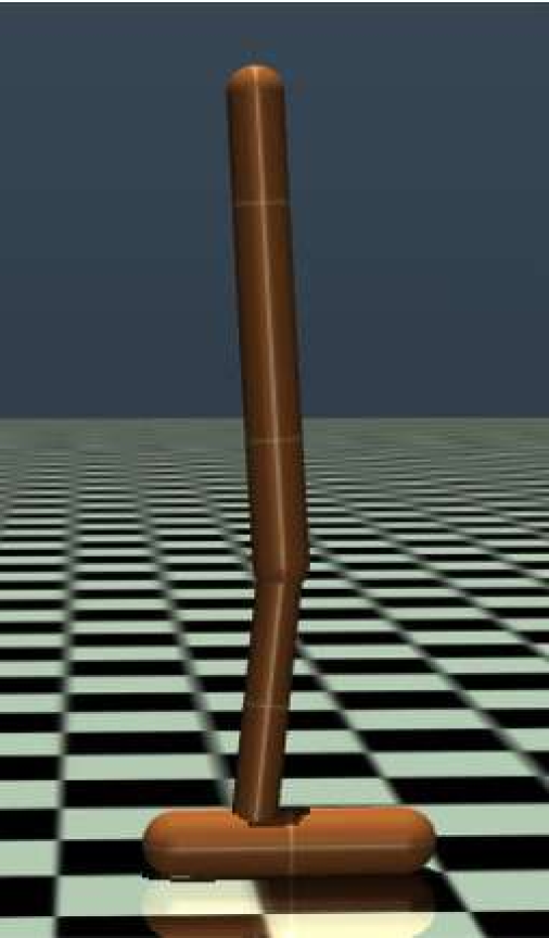
(a) Hopper

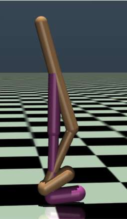
(b) Walker2d

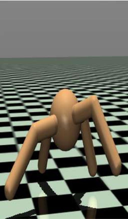
(c) Ant

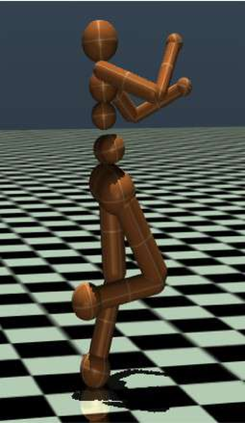
(d) Humanoid

Figure 8: Four OpenAI Gym locomotion Tasks: Hopper, Walker2d, Ant, and Humanoid.

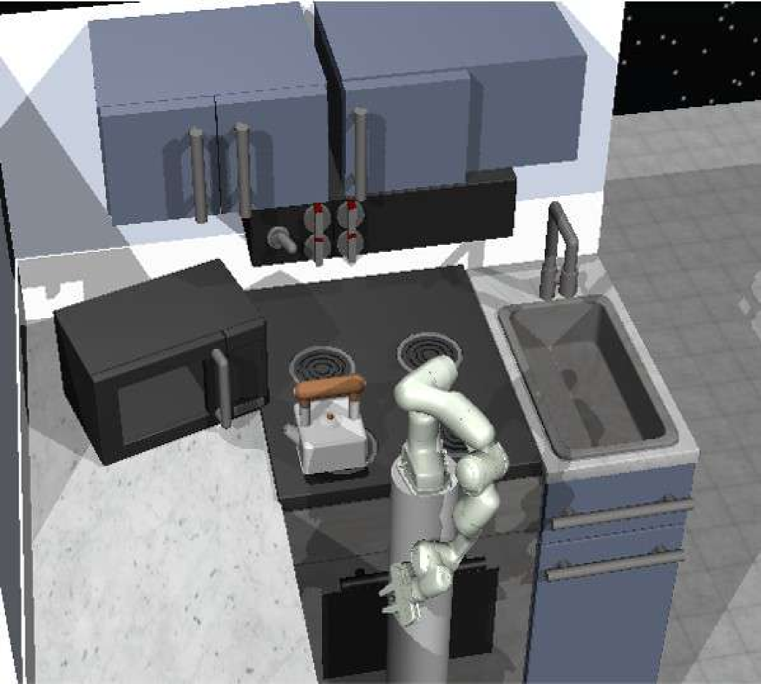
(a) Franka Kitchen

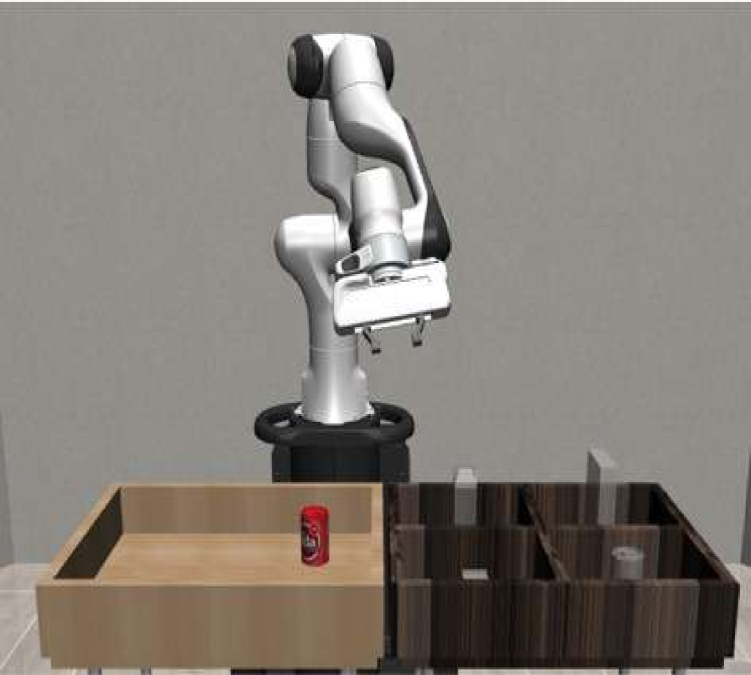
(b) PickPlaceCan

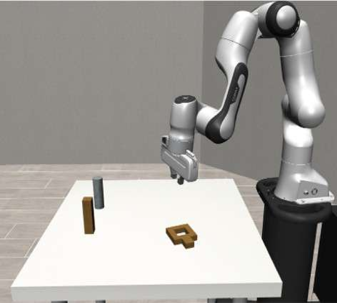
(c) NutAssemblySquare

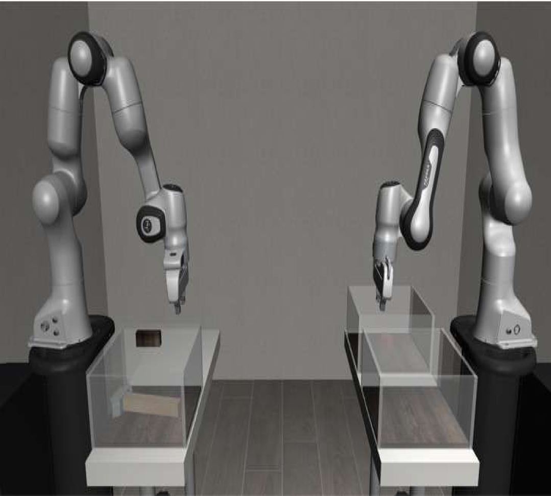
(d) TwoArmTransport

Figure 9: Four manipulation tasks in state-input Franka Kitchen and pixel-input Robomimic environments.

Environment Configuration.

We also list the environment configurations in different tasks in Table 1.

Table 1: Environment Configuration

Environment	Task or Dataset	State Dim	Image Shape	Action Chunk	Max. Eps. Len.$H$	Reward
OpenAI Gym	Hopper-v2	11	-	3 $\times$ 4	1000	Dense
	Walker2d-v2	17	-	6 $\times$ 4	1000	Dense
	Ant-v0	111	-	8 $\times$ 4	1000	Dense
	Humanoid-v3	376	-	17 $\times$ 4	1000	Dense
Franka Kitchen	Kitchen-Complete-v0	60	-	9 $\times$ 4	280	Sparse
	Kitchen-Mixed-v0	60	-	9 $\times$ 4	280	Sparse
	Kitchen-Partial-v0	60	-	9 $\times$ 4	280	Sparse
Robomimic	Can	9	[3,96,96] $\times$ 1	7 $\times$ 4	300	Sparse
	Square	9	[3,96,96] $\times$ 1	7 $\times$ 4	400	Sparse
	Transport	18	[3,96,96] $\times$ 2	14 $\times$ 8	800	Sparse

In Tab. 1, the “State Dim” indicates the dimension of proprioception inputs. “Action Chunk” expresses the dimension of a single action and the size of the action chunk. “Max.Eps.Len. $H$” indicates the maximum steps a robot can take in a single rollout. When the reward is “sparse, we award the agent a reward of $+1$ only upon task completion. Otherwise, the agent receives a $0$ reward. The sparse reward is realistic, straightforward, and directly associated with the success rate of manipulation tasks. A “dense” reward system assigns the reward based on the robot’s dynamics and kinematic properties. It is usually a floating number after each step of action execution. Dense reward systems need careful design. We adopt them primarily in sim2real training for legged locomotion tasks.

The Robomimic Dataset Provided by DPPO [43]

We remark that, in Robomimic environments, we adhere to the configuration of DPPO [43], which makes the shapes of the state vector smaller than the official default implementation in [37]. This processing simplifies robot learning and makes the pre-trained data provided by [43] smaller and simpler than Robomimic’s official datasets. As acknowledged by the authors of DPPO, the datasets provided by [43] are of lower quality and/or quantity than the official release, so the pre-trained policy is trained on inferior data. Consequently, the pre-trained checkpoints of both DDPM and Shortcut policies have a lower success rate than the best-reported results in the literature [19].

We can train flow matching or diffusion policies with RoboMimic’s default configuration and datasets, which will help us align with state-of-the-art results in the imitation learning literature. However, we may need to adopt larger neural networks and spend more time pre-training and fine-tuning.

Datasets for OpenAI Gym Tasks

To faithfully replicate the results of DPPO [43], we trained both DPPO and ReinFlow agents using the behavior cloning (BC) dataset provided by Ren et al. (2024) [43]. For consistency, we followed their dataset choices for all experiments in the Appendix that do not involve offline reinforcement learning (RL) algorithms, such as FQL.

However, the DPPO dataset for OpenAI Gym tasks lacks the offline rewards necessary to train an FQL agent, and the authors did not specify how they constructed their Gym dataset. We hypothesize that their BC datasets were derived and augmented from D4RL [20]. Therefore, in the experiments that involve FQL (described in Section 5.2 of the main text), we adopted D4RL offline RL datasets to train DPPO, FQL, and ReinFlow agents. We also remark that while we chose the “Ant-v2” environment in these experiments, we switched to “Ant-v0” in the sensitivity analysis in Section 4.3 and the Appendix.

The minor differences in OpenAI Gym Tasks mentioned above resulted in minimal discrepancy in reward curves.

Appendix D Implementation Details

D.1 Model Architecture

For a fair comparison, we try to make the model architecture of flow matching policies align with diffusion policies proposed in DPPO [43] as much as possible.

State-input Tasks.

In state-input tasks (OpenAI Gym and Franka Kitchen), the velocity nets $v_{\theta}$ of 1-ReFlow policies are parameterized with Multi-layer Perceptrons (MLP) that receive action chunk, state, and time features. The time input $t\in(0,1)$ is encoded by sinusoidal positional embedding [26] and linear projections, with a Mish [38] activation function in between. We implement Shortcut Models similarly, passing the time and inference step counts through the same sinusoidal positional embedding and concatenating. At the same time, we also encode the state input with a small MLP and add the state feature with the time-step features. The sizes of Shortcut Models are often slightly smaller than 1-ReFlow policies in the same task. Critic networks are also MLPs with the same or half the width.

Pixel-input Tasks.

In Robomimic, where the agent receives pixel and proprioception inputs, the actor and the critic adopt a single-layer Visual Transformer [16] with random shift augmentation as the visual encoder and compresses the proprioception information with a small MLP. We pass the features of the visuomotor condition, time embedding, and the raw action chunk through the actor’s velocity head, which outputs a velocity estimate. The critic only receives features from time and condition.

Noise-injection Net

The noise injection network $\theta^{\prime}$ shares the input features with the actor and outputs the standard deviation of the noise at each coordinate of the actions in the action chunk. The output of network $\theta^{\prime}$ is passed through a $\mathrm{Tanh}$ function coupled with affine transform, to ensure bounded output and smooth gradients. The upper and lower bounds of the noise standard deviation $\sigma_{\max},\sigma_{\min}$ are a group of essential hyperparameters of ReinFlow, and we have provided an analysis in Section 6 to study how they influence exploration.

We discard $\sigma_{\theta^{\prime}}$ after fine-tuning. Although a noise-injected process exists during RL, ReinFlow still returns a policy with an ODE inference path.

During the evaluation, we also did not inject noise into the flow policy; We observed that the reward is often higher than the noise-injected version, aligning with findings in classical RL literature [23].

Parameter Scale

We summarize the sizes of the actor, critic, and noise injection networks in Table 2, which shows that for state-input tasks, a negligible parameter increase ($<6\%$) brought by the noise injection network returns promises a 135.36%  net increase in reward and a 31.29% net increase in success rate.

For complex visual manipulation tasks beyond robomimic, since the noise network $\theta^{\prime}$ shares the same representation backbone as the velocity network, the parameter increase should also remain minimal when scaling to larger models with more complex backbones, such as multi-layer Transformers, instead of the single-layer Transformer used in our experiments.

Designing an efficient noise injection network architecture that balances reward improvement and parameter count is an interesting problem, which we leave for future work.

Table 2: Model Parameter Counts

Task	Model	Pre-trained Actor $\theta$/M	Noise Net $\theta^{\prime}$/M	Fine-tuned Actor $\bar{\theta}$/M	Critic /M	Total /M	Noise/ Velocity
Hopper-v2	1-ReFlow	0.55	0.01	0.56	0.13	0.69	1.22%
Walker2d-v2	1-ReFlow	0.57	0.01	0.58	0.14	0.71	1.39%
Ant-v3	1-ReFlow	0.62	0.01	0.64	0.16	0.80	2.31%
Humanoid-v3	1-ReFlow	0.80	0.03	0.83	0.23	1.06	4.23%
Kitchen	Shortcut	0.16	0.01	0.17	0.15	0.31	5.46%
Can	Shortcut	1.01	0.15	1.16	0.59	1.74	14.59%
Square	Shortcut	1.69	0.32	2.01	0.59	2.59	18.91%
Transport	Shortcut	1.87	0.35	2.22	0.66	2.87	18.84%

D.2 Enhancing Training Stability

Clipping probability ratio

For stability reasons, we clip the log probability ratio in Algorithm 1 with $\epsilon=0.01$ for state-input tasks and $\epsilon=0.001$ for pixel-input tasks. This choice follows DPPO [43].

Clipping denoised actions

Although unnecessary for the pre-trained flow policies, we discover that during fine-tuning, it is beneficial to clip the denoised actions of a flow matching policy because this helps prevent the injected noise from interrupting the integration path too violently. After fine-tuning with ReinFlow, policies should also clip the denoised actions during inference; otherwise, performance may likely deteriorate.

Critic Warmup

Training the critic network for several iterations before updating the actor is crucial for stable training and rapid convergence, particularly for larger models with visual inputs. We refer to this phase as “critic warm-up”. Since we use RL as a fine-tuning approach, the critic should output a reasonably large value (at least positive) before the policy gradient starts. An excessively small or even negative initial output misleads the actor into considering its current actions as excessively unsatisfying, resulting in rapidly degrading rewards and value function estimates during the fine-tuning process.

Empirically, we recommend initializing the critic and/or adjusting the critic warm-up iteration number according to the initial reward of the pre-trained policy, the rollout step number, and the discount factor.

Critic Overfitting and Initialization

An excessively long warm-up period may lead to overfitting of the critic network, especially in cases where the critic is significantly smaller than the pre-trained policy (Table 2). When the critic overfits, the policy gradient loss could oscillate violently during fine-tuning.

One possible solution to address critic overfitting is to incorporate regularizations into the critic’s training procedure. Another method is to limit the warm-up iterations and initialize the critic’s last fully connected layer with a positive bias. The bias can be estimated by the pre-trained success rate. With a positive initial output, the critic requires fewer warm-up iterations to output an appropriate value estimate without overfitting the pre-trained policy’s distributions.

Appendix E Additional Experimental Results

Random seeds

Unless specified, we train all the RL algorithms with seeds 0, 42, and 3407 for all tasks except for Franka Kitchen with mixed or partial data, where we adopt two extra seeds, 509 and 2025, in the main experiment section 5. These tasks involve long-horizon multi-task planning, and we discover that DPPO and ReinFlow exhibit high variations across different runs.

The RL fine-tuning curves show the reward or success rate averaged over these seeds, with shading representing the mean ± standard deviation to indicate variability across runs.

Rendering Backend

During training and wall time testing, the MuJoCo graphics rendering backend ($\mathrm{MUJOCO\_GL}$) is set to Embedded System Graphics Library ($\mathrm{EGL}$) to accelerate the computation with GPU. If users do not have EGL support and they switch to software rendering ($\mathrm{osmesa}$), or if multiple threads are running together on the same group of CPU kernels or the same GPU, the compute time may be longer than that described in Table 3.

Wall-clock Time

Table 3: Per Iteration Wall-clock Time

Task	Algorithm	Single Iteration Time/second			Average
		seed=0	seed=42	seed=3407	Mean $\pm$ Std
Hopper-v2	ReinFlow-R	11.598	11.704	11.843	11.715 $\pm$ 0.123
	ReinFlow-S	12.051	12.127	12.372	12.290 $\pm$ 0.141
	DPPO	99.502	99.616	98.021	99.046 $\pm$ 0.890
	FQL	4.373	4.366	4.515	4.418 $\pm$ 0.084
Walker2d-v2	ReinFlow-R	11.861	11.446	11.382	11.563 $\pm$ 0.260
	ReinFlow-S	12.393	12.690	13.975	13.019 $\pm$ 0.841
	DPPO	101.151	106.125	98.470	101.915 $\pm$ 3.884
	FQL	5.248	4.597	5.207	5.017 $\pm$ 0.365
Ant-v0	ReinFlow-R	17.210	17.685	17.524	17.473 $\pm$ 0.242
	ReinFlow-S	17.291	17.821	18.090	17.734 $\pm$ 0.407
	DPPO	102.362	104.632	99.042	102.012 $\pm$ 2.811
	FQL	5.242	4.950	5.3086	5.167 $\pm$ 0.191
Humanoid-v3	ReinFlow-R	31.437	30.223	31.088	30.916 $\pm$ 0.625
	ReinFlow-S	30.499	30.058	31.029	30.529 $\pm$ 0.486
	DPPO	109.884	105.455	113.358	109.566 $\pm$ 3.961
	FQL	5.245	4.981	5.522	5.249 $\pm$ 0.271
Franka Kitchen	ReinFlow-S	26.655	26.328	26.628	26.537 $\pm$ 0.182
	DPPO	81.584	84.646	83.245	83.158 $\pm$ 1.533
	FQL	5.245	4.981	5.522	5.249 $\pm$ 0.271
Can (image)	ReinFlow-S	219.943	216.529	217.711	218.061 $\pm$ 1.734
	DPPO	310.974	307.811	308.014	308.933 $\pm$ 1.771
Square (image)	ReinFlow-S	313.457	312.3	313.862	313.206 $\pm$ 0.811
	DPPO	438.506	440.212	434.773	437.830 $\pm$ 2.782
Transport (image)	ReinFlow-S	554.196	557.712	559.006	558.359 $\pm$ 0.915
	DPPO	406.607	439.268	412.077	419.317 $\pm$ 17.493

For a fair comparison, we measure all algorithms’ wall-clock time in all the tasks (except Transport) on a single NVIDIA RTX 3090 GPU with EGL rendering. We evaluate the wall time of Robomimic Transport on two NVIDIA A100 GPUs with EGL rendering, as this task occupies significantly more memory than a single RTX 3090 GPU. The measurement is taken sequentially for three random seeds without interfering with other processes. We obtain the total wall-clock time for each algorithm by multiplying the average iteration time by the number of iterations. Table 3 provides a detailed record of these measurements, where the results are recorded in seconds and accurate to three decimal places.

Although FQL’s per-iteration wall time is significantly shorter than other methods, this does not imply that it is more efficient overall: FQL’s batch size is considerably smaller than that of PPO-based methods, including ReinFlow and DPPO, and its total training iterations are significantly larger than those of the other two methods; neither is FQL designed for parallel computing like DPPO and ReinFlow.

Performance Increase

We report the performance improvement after fine-tuning flow matching policies with ReinFlow across various simulation tasks in Table 4.

For locomotion tasks, we compute the reward increase ratio as follows:

$$\text{Locomotion Reward Net Increase Ratio}=\frac{\text{Fine-tuned Reward}-\text{Fine-tuned Reward}}{\text{Pre-trained Reward}}$$ (26)

For manipulation tasks, we compute the success rate increase:

$$\text{Manipulation Success Rate Net Increase}=\text{Fine-tuned Success Rate}-\text{Pre-trained Success Rate}$$ (27)

Policies fine-tuned with ReinFlow achieved an average episode reward net increase of $\mathbf{135.36}\%$ in OpenAI Gym locomotion tasks using D4RL datasets, with an average success rate increase of $\mathbf{31.29}\%$ in Franka Kitchen, $\mathbf{45.77}\%$ in Robomimic, and $\mathbf{40.34}\%$ in all manipulation tasks. The results are accurate to two decimal places.

Table 4: Performance Metrics for ReinFlow Across Tasks.

(a) Average Episode Reward in Locomotion Tasks.

Task	Algorithm	Pre-trained Episode Reward	Fine-tuned Episode Reward	Reward Net Increase Ratio
Hopper-v2	ReinFlow-R	1431.80±27.57	3205.33±32.09	123.87%
	ReinFlow-S	1528.34±14.91	3283.27±27.48	114.83%
Walker2d-v2	ReinFlow-R	2739.90±74.57	4108.57±51.77	49.95%
	ReinFlow-S	2739.19±134.30	4254.87±56.56	55.33%
Ant-v2	ReinFlow-R	1230.54±8.18	4009.18±44.60	225.81%
	ReinFlow-S	2088.06±79.34	4106.31±79.45	225.81%
Humanoid-v3	ReinFlow-R	1926.48±41.48	5076.12±37.47	163.49%
	ReinFlow-S	2122.03±105.01	4748.55±70.71	123.77%

(b) Average Success Rate in Manipulation Tasks.

Environment and Task	Algorithm	Pre-trained Success Rate	Fine-tuned Success Rate	Success Rate Net Increase
Kitchen-complete	ReinFlow-S	73.16±0.84%	96.17±3.65%	23.01%
Kitchen-mixed	ReinFlow-S	48.37±0.78%	74.63±0.36%	26.26%
Kitchen-partial	ReinFlow-S	40.00±0.28%	84.59±12.38%	44.59%
Can (image)	ReinFlow-R	59.00±3.08%	98.67±0.47%	39.67%
	ReinFlow-S	57.83±1.25%	98.50±0.71%	40.67%
Square (image)	ReinFlow-R	25.00±1.47%	74.83±0.24%	49.83%
	ReinFlow-S	34.50±1.22%	74.67±2.66%	40.17%
Transport (image)	ReinFlow-S	30.17±2.46%	88.67±4.40%	58.50%

Sample Complexity in Gym Tasks

Here, we also compare the sample complexity in OpenAI Gym tasks omitted in the main text.

H

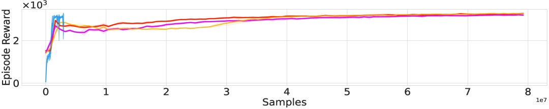
(a) Hopper-v2

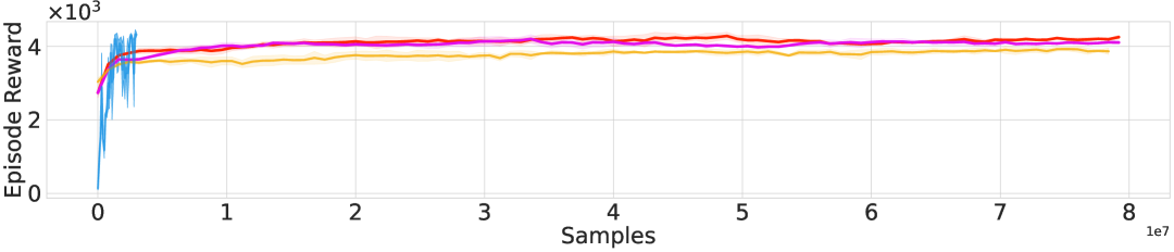
(b) Walker2d-v2

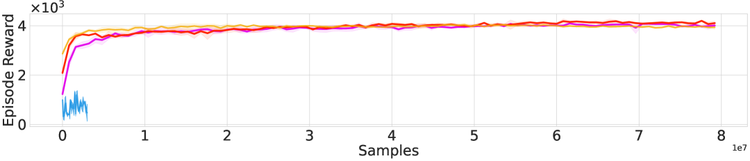
(c) Ant-v2

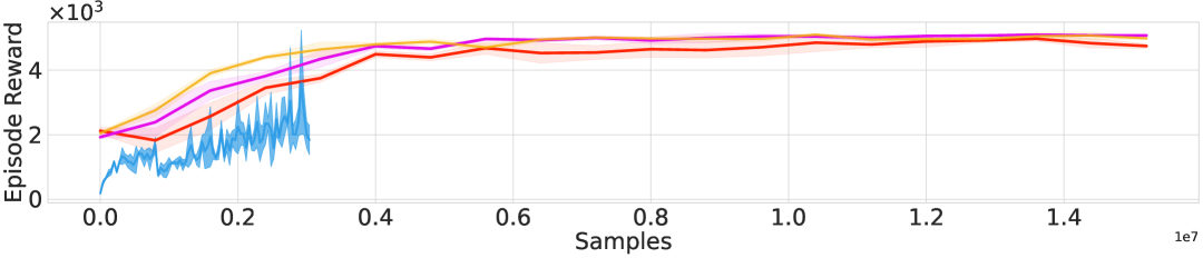
(d) Humanoid-v3

Figure 10: Sample efficiency results of state-based locomotion tasks in OpenAI Gym. For better visualization, we down-sampled FQL’s data by five times in the first three tasks and three times in “Humanoid-v3”. Although FQL is more sample-efficient than DPPO and ReinFlow in simpler tasks, it struggles to achieve high reward in more challenging locomotion tasks.

While FQL is more sample efficient in simpler tasks such as Hopper and Walker2d, it generally struggles to tackle more complex locomotion task, where it is asymptotically inferior to DPPO and ReinFlow.

Comparison with Other Diffusion RL Methods

We compare the diffusion RL baselines with our method in a few representative continuous control tasks. For these baselines, we adopt the same set of hyperparameters described in [43].

Figs 11 and 12 show that ReinFlow overall outperforms other methods concerning the stability w.r.t random seeds and asymptotic performance.

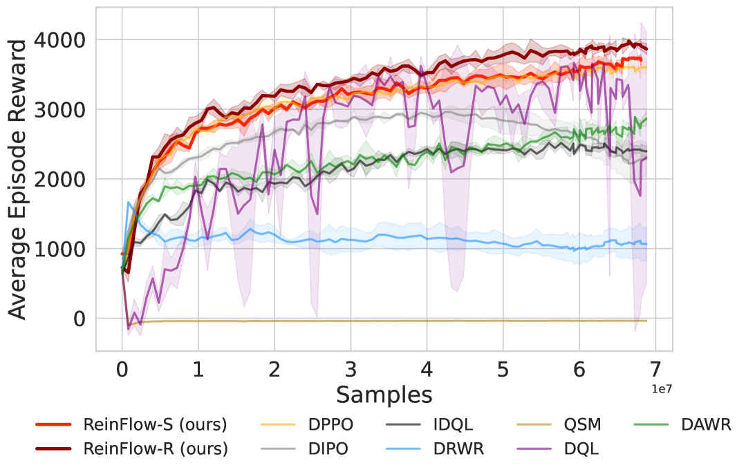
Figure 11: Fine-tuning locomotion task Ant-v0 with Diffusion RL baselines and ReinFlow.

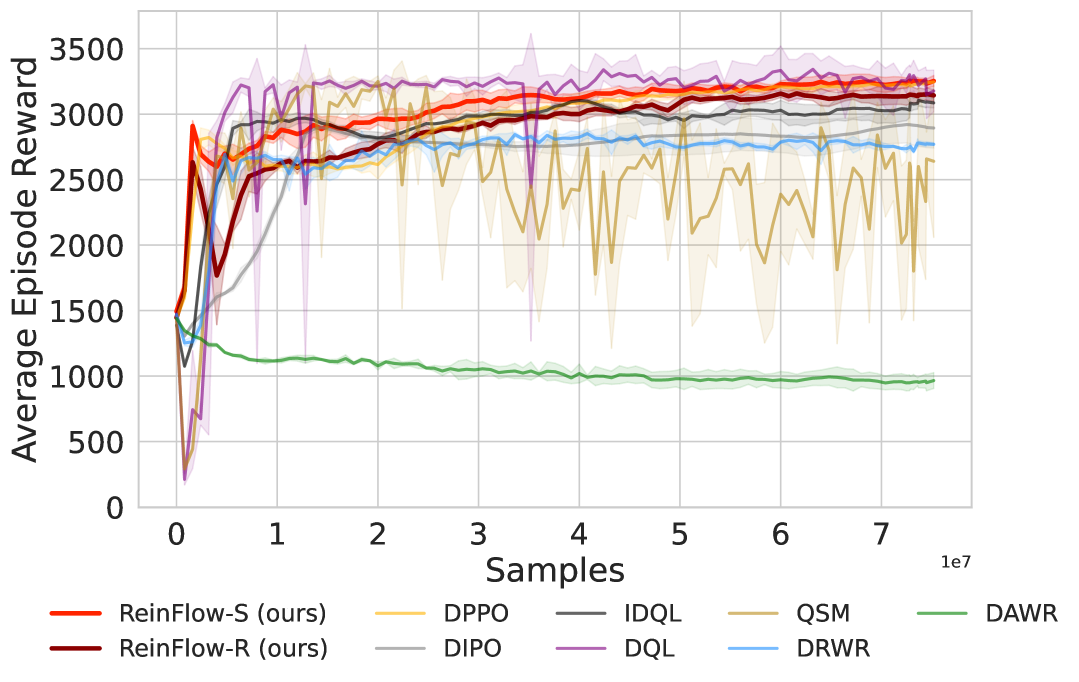
(a) Hopper-v2

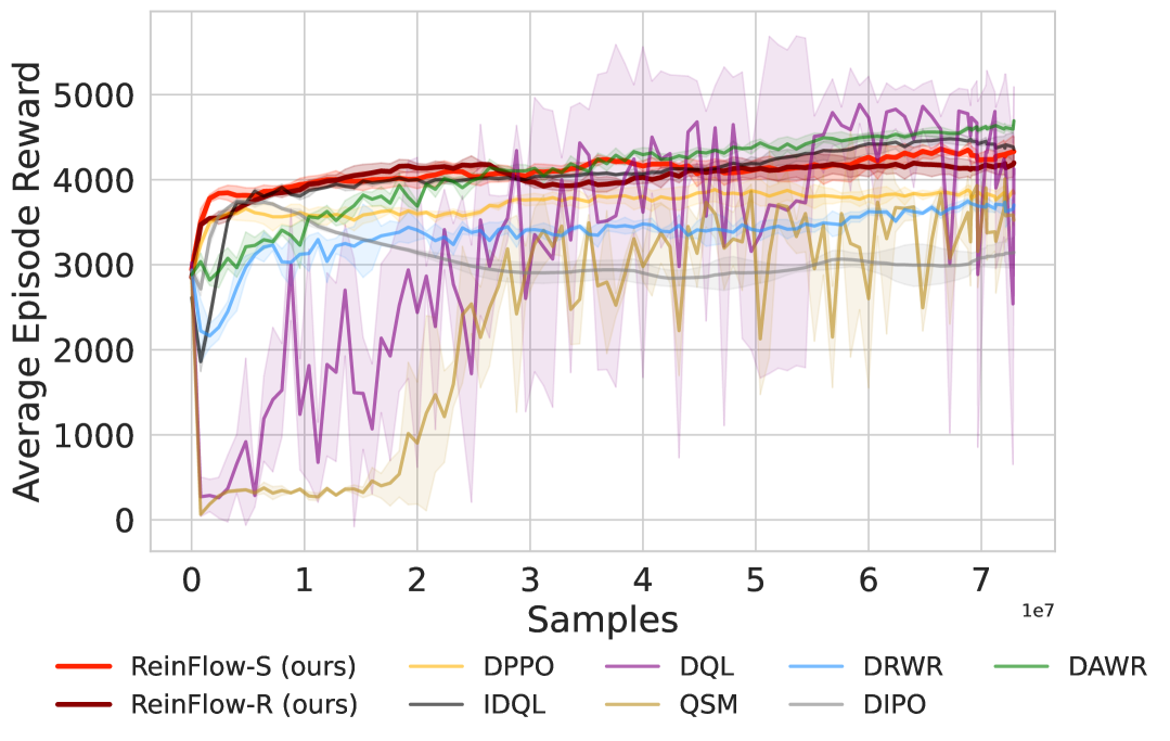
(b) Walker2d-v2

Figure 12: Fine-tuning locomotion task Hopper-v2 and Walker2d-v2 with Diffusion RL baselines and ReinFlow.

Changing the Behavior Cloning Dataset’s Scale in Square

Tab. 5 shows how the fine-tuned performance of ReinFlow is affected by the scale of the behavior cloning dataset in robomimic square. Fine-tuning the policy trained on 16 episodes failed due to an overly low initial success rate. We adopt the same hyperparameter set when fine-tuning policies trained on 64 and 100 episodes, restricting the noise standard deviation to $\mathrm{std}\in[0.08,0.14]$ with entropy coefficient $0.01$. We slightly tuned down the noise to $\mathrm{std}\in[0.06,0.10]$ and removed entropy regularization, as we find it is more beneficial to limit exploration when the pre-trained policy performs poorly.

Table 5: Fine-tuned Success Rates in Square Across Different Pre-trained Episodes

Pre-trained Episodes	Pre-trained Success Rate	Fine-tuned Success Rate			Average Fine-tuned Success Rate
		seed=42	seed=0	seed=3407	Mean	Std
16	3.08 %	0.00 %	0.00 %	0.00 %	3.08 %	0.00 %
32	10.15%	22.20%	22.00%	18.50%	20.90%	1.70 %
64	27.67%	65.50%	62.20%	56.20%	61.30%	3.85 %
100	25.14%	79.50%	78.20%	74.50%	77.40%	2.12 %

Changing the Number of Fine-tuned Denoising Steps

Altering the fine-tuned denoising step number $K$ could affect ReinFlow’s performance since the pre-trained policy has different rewards when evaluated at different steps.

Fig. 13 shows the difference when fine-tuning a Shortcut Policy in Franka Kitchen at $K=1,2,$ and $4$ denoising steps.

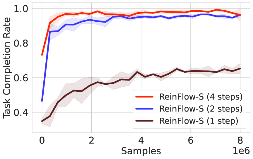
Figure 13: Fine-tuning Shortcut Policy in Kitchen-complete-v0 at Different Denoising Steps $1,2,$ and $4$. The result averaged over three seeds $0,42,3407$.

In Fig. 13, all the run hyperparameters except $K$ and random seeds are the same. The pre-trained policy adopts complete demonstration data.

Increasing $K$ improves the reward at the beginning of fine-tuning. A better starting point shrinks the space of exploration and thus accelerates convergence. However, a longer denoising trajectory also consumes more simulation time. Fig. 13 and Fig. 4(a) also show that the success rate or episode reward quickly plateaus when scaling $K$.

In more challenging tasks such as visual manipulation, we also find that reducing the noise standard deviation is beneficial when we increase the number of denoising steps $K$, especially when the pre-trained policy has a low success rate.

Appendix F Reproducing Our Findings

We list the key hyper-parameters and model architectures needed to reproduce the experiment results of ReinFlow and other baseline algorithms.

F.1 Hyperparameters of ReinFlow

We adopt the same batch size suggested in DPPO [43] and follow their implementation to normalize the reward with time-reversed running variance.

It is essential to adjust the number of critic warmup iterations according to the performance of the pre-trained policy. A larger initial reward requires more warmup steps.

We clipped the denoised actions within $[-1,1]$ to enhance training stability in implementation. Table 7 indicates this option with “clip intermediate actions”. We also find it beneficial to slightly reduce the maximum noise standard deviation in the latter training course to postpone the reward decrease. $\mathrm{cos}(r_{1},r_{2})$ indicates a learning rate that decays in the rate of a cosine function from $r_{1}$ to $r_{2}$.

Table 6: ReinFlow’s Shared Hyperparameters Across All Tasks

Parameter	Value
critic loss coefficient	0.50
GAE lambda $\lambda$	0.95
reward scale	1.0
reward normalization	True
actor optimizer	Adam [27]
actor learning rate weight decay	0
actor learning rate scheduler	CosineAnnealingWarmupRestart [36]
actor learning rate cycle steps	100
critic optimizer	Adam
critic learning rate scheduler	CosineAnnealingWarmupRestart
critic scheduler warmup	10
critic learning rate cycle steps	100

Table 7: ReinFlow’s Hyperparameters in OpenAI Gym Locomotion Tasks

(a) Shared Hyperparameters Across OpenAI Gym Tasks

Parameter	Value
critic learning rate weight decay	1e-5
number of parallel environments	40
reward discount factor $\gamma$	0.99
action chunking size	4
condition stacking number	1
batch size	50k
maximum episode steps	1000
number of rollout steps	500
update epochs	5
number of training iterations	1000
number of denoising steps	4
clipping ratio $\epsilon$	0.01
clip intermediate actions	True
target KL divergence	1.0
noise std upper bound hold for	35% of total iteration
noise std upper bound decay to	$0.3\times\sigma_{\mathrm{min}}+0.7\times\sigma_{\mathrm{max}}$
entropy coefficient $\alpha$	0.03
BC loss ($W_{2}$ regularization) coefficient $\beta$	0.00

(b) Task-Specific Hyperparameters in OpenAI Gym Environment

Parameter	Hopper-v2	Walker2d-v2	Ant-v0 Humanoid-v3
minimum noise std $\sigma_{\mathrm{min}}$	0.10	0.10	0.08
maximum noise std $\sigma_{\mathrm{max}}$	0.24	0.24	0.16
critic warmup iters	0	5	0
actor learning rate	cos(4.5e-5, 2.0e-5)	cos(4.5e-4, 4.0e-4)	cos(4.5e-5, 2.0e-5)
critic learning rate	cos(6.5e-4, 3.0e-4)	cos(4.0e-3, 4.0e-3)	cos(6.5e-4, 3.0e-4)

Table 8: ReinFlow’s Hyperparameters in Franka Kitchen State-input Manipulation Tasks

Parameter	Value
critic learning rate weight decay	1e-5
number of parallel environments	40
reward discount factor $\gamma$	0.99
action chunking size	4
condition stacking number	1
batch size	5600
maximum episode steps	280
number of rollout steps	200
update epochs	10
number of training iterations	301
number of denoising steps	4
clipping ratio $\epsilon$	0.01
clip intermediate actions	True
minimum noise std $\sigma_{\mathrm{min}}$	0.05
maximum noise std $\sigma_{\mathrm{max}}$	0.12
noise std upper bound hold for	100% of total iteration
noise std upper bound decay to	$\sigma_{\mathrm{max}}$
entropy regularization coefficient $\alpha$	0.00
BC loss ($W_{2}$ regularization) coefficient $\beta$	0.00

Table 9: ReinFlow’s Hyperparameters in Robomimic Visual Manipulation Tasks

(a) Shared Hyperparameters Across Robomimic Tasks

Parameter	Value
critic learning rate weight decay	0
number of parallel environments	50
reward discount factor $\gamma$	0.999
condition stacking number	1
pixel input shape	[3, 96, 96]
image augmentation	RandomShift (padding=4)
gradient accumulation steps	15
batch size	500
update epochs	10
clipping ratio $\epsilon$	0.001
clip intermediate actions	True
target KL divergence	1e-2
noise std upper bound hold for	100% of total iteration
noise std upper bound decay to	$\sigma_{\mathrm{max}}$
BC loss ($W_{2}$ regularization) coefficient $\beta$	0.00

(b) Task-Specific Hyperparameters in Robomimic Environment

Parameter	PickPlaceCan	NutAssemblySquare	TwoArmTransport
minimum noise std $\sigma_{\mathrm{min}}$	0.08	0.08	0.05
maximum noise std $\sigma_{\mathrm{max}}$	0.14	0.14	0.10
number of denoising steps	1	1	4
entropy coefficient $\alpha$	0.00	0.01	0.00
critic warmup iters	2	2	5
critic output layer bias	0.0	0.0	4.0
actor learning rate warmup	10	25	10
actor learning rate	cos(2.0e-5, 1.0e-5)	cos(3.5e-6, 3.5e-6)	cos(3.5e-5, 3.5e-5)
critic learning rate	cos(6.5e-4, 3.0e-4)	cos(4.5e-4, 3.0e-4)	cos(3.2e-4, 3.0e-4)
action chunking size	4	4	8
number of cameras	1	1	2
maximum episode steps	300	400	800
number of rollout steps	300	400	400
number of training iterations	150	300	200

F.2 Hyperparameters of DPPO

We strictly follow the hyperparameter setting of the official implementation of DPPO. Please refer to Section E.10 of [43] for details.

The only changes we make are incorporating seeds $509$ and $2025$ for furniture tasks and elongating the rollout steps from $70$ to $200$ (while we still keep the maximum episode length as $280$ in the environment configuration). DPPO and ReinFlow exhibit higher variability in Franka kitchen tasks across random seeds and even different runs, so we adopt five random seeds. We also find that a longer sampling trajectory helps the DPPO agent discover optimal strategies. For this reason, DPPO achieves a higher task completion rate than that reported by DPPO’s original paper.

F.3 Hyperparameters of FQL

We list the hyperparameters adopted by FQL in Table 10. We set the number of offline pre-training steps such that the total sample consumption during the offline phase is no less than the pre-trained consumption of DPPO or ReinFlow in Gym (D4RL) and Franka Kitchen tasks.

As described in [39], the temperature coefficient, $\alpha_{\mathrm{FQL}}$, is the most important hyperparametero f FQL. We followed the instructions of the original paper and scanned $\alpha_{\mathrm{FQL}}$ in $[0.03,0.1,0.3,1,3,10]$ to obtain a proper value for the temperature in Hopper-v2. and adopted the same value for all state-input tasks.

Table 10: Hyperparameters for FQL in Gym and Franka Kitchen Tasks

(a) Shared Hyperparameters for FQL

Parameter	Value
number of denoising steps of the base policy $\pi_{\theta}$	4
number of steps for evaluation	500
number of evaluation episodes	10
reward discount factor $\gamma$	0.99
actor learning rate	$1e-4$
actor weight decay	0
actor learning rate cycle steps	1000
actor scheduler warmup	10
critic learning rate	$3e{-4}$
critic learning rate weight decay	0
critic scheduler warmup	10
batch size	256
target EMA rate	0.005
reward scale	1.0
buffer size	$1e6$
Behavior cloning coefficient	3.0
actor update repeat	1
online steps	569,936

(b) Task-Specific Hyperparameters in Robomimic Environment

Parameter	Gym and Kitchen-complete-v0	Kitchen-mixed-v0 and Kitchen-partial-v0
offline steps	200,000	600,000

References

- [1] A. Agarwal, N. Jiang, S. M. Kakade, and W. Sun. Reinforcement learning: Theory and algorithms. CS Dept., UW Seattle, Seattle, WA, USA, Tech. Rep, 32, 2019.
- [2] A. Agarwal, S. M. Kakade, J. D. Lee, and G. Mahajan. On the theory of policy gradient methods: Optimality, approximation, and distribution shift. Journal of Machine Learning Research, 22(98):1–76, 2021.
- [3] L. Ankile, A. Simeonov, I. Shenfeld, and P. Agrawal. Juicer: Data-efficient imitation learning for robotic assembly, 2024.
- [4] M. Arjovsky, S. Chintala, and L. Bottou. Wasserstein generative adversarial networks. In D. Precup and Y. W. Teh, editors, Proceedings of the 34th International Conference on Machine Learning, volume 70 of Proceedings of Machine Learning Research, pages 214–223. PMLR, 06–11 Aug 2017.
- [5] S. Belkhale, Y. Cui, and D. Sadigh. Data quality in imitation learning. In A. Oh, T. Naumann, A. Globerson, K. Saenko, M. Hardt, and S. Levine, editors, Advances in Neural Information Processing Systems, volume 36, pages 80375–80395. Curran Associates, Inc., 2023.
- [6] K. Black, N. Brown, D. Driess, A. Esmail, M. Equi, C. Finn, N. Fusai, L. Groom, K. Hausman, B. Ichter, S. Jakubczak, T. Jones, L. Ke, S. Levine, A. Li-Bell, M. Mothukuri, S. Nair, K. Pertsch, L. X. Shi, J. Tanner, Q. Vuong, A. Walling, H. Wang, and U. Zhilinsky. : A vision-language-action flow model for general robot control, 2024.
- [7] K. Black, N. Brown, D. Driess, A. Esmail, M. Equi, C. Finn, N. Fusai, L. Groom, K. Hausman, B. Ichter, S. Jakubczak, T. Jones, L. Ke, S. Levine, A. Li-Bell, M. Mothukuri, S. Nair, K. Pertsch, L. X. Shi, J. Tanner, Q. Vuong, A. Walling, H. Wang, and U. Zhilinsky. : A vision-language-action flow model for general robot control, 2024.
- [8] M. Braun, N. Jaquier, L. Rozo, and T. Asfour. Riemannian flow matching policy for robot motion learning. In 2024 IEEE/RSJ International Conference on Intelligent Robots and Systems (IROS), pages 5144–5151, 2024.
- [9] G. Brockman, V. Cheung, L. Pettersson, J. Schneider, J. Schulman, J. Tang, and W. Zaremba. Openai gym, 2016.
- [10] S. Cen, C. Cheng, Y. Chen, Y. Wei, and Y. Chi. Fast global convergence of natural policy gradient methods with entropy regularization. Oper. Res., 70(4):2563–2578, July 2022.
- [11] R. T. Q. Chen, Y. Rubanova, J. Bettencourt, and D. K. Duvenaud. Neural ordinary differential equations. In S. Bengio, H. Wallach, H. Larochelle, K. Grauman, N. Cesa-Bianchi, and R. Garnett, editors, Advances in Neural Information Processing Systems, volume 31. Curran Associates, Inc., 2018.
- [12] C. Chi, Z. Xu, S. Feng, E. Cousineau, Y. Du, B. Burchfiel, R. Tedrake, and S. Song. Diffusion policy: Visuomotor policy learning via action diffusion, 2024.
- [13] O. X.-E. Collaboration, A. O’Neill, A. Rehman, A. Gupta, A. Maddukuri, A. Gupta, A. Padalkar, A. Lee, A. Pooley, A. Gupta, A. Mandlekar, A. Jain, A. Tung, A. Bewley, A. Herzog, A. Irpan, A. Khazatsky, A. Rai, A. Gupta, A. Wang, A. Kolobov, A. Singh, A. Garg, A. Kembhavi, A. Xie, A. Brohan, A. Raffin, A. Sharma, A. Yavary, A. Jain, A. Balakrishna, A. Wahid, B. Burgess-Limerick, B. Kim, B. Schölkopf, B. Wulfe, B. Ichter, C. Lu, C. Xu, C. Le, C. Finn, C. Wang, C. Xu, C. Chi, C. Huang, C. Chan, C. Agia, C. Pan, C. Fu, C. Devin, D. Xu, D. Morton, D. Driess, D. Chen, D. Pathak, D. Shah, D. Büchler, D. Jayaraman, D. Kalashnikov, D. Sadigh, E. Johns, E. Foster, F. Liu, F. Ceola, F. Xia, F. Zhao, F. V. Frujeri, F. Stulp, G. Zhou, G. S. Sukhatme, G. Salhotra, G. Yan, G. Feng, G. Schiavi, G. Berseth, G. Kahn, G. Yang, G. Wang, H. Su, H.-S. Fang, H. Shi, H. Bao, H. B. Amor, H. I. Christensen, H. Furuta, H. Bharadhwaj, H. Walke, H. Fang, H. Ha, I. Mordatch, I. Radosavovic, I. Leal, J. Liang, J. Abou-Chakra, J. Kim, J. Drake, J. Peters, J. Schneider, J. Hsu, J. Vakil, J. Bohg, J. Bingham, J. Wu, J. Gao, J. Hu, J. Wu, J. Wu, J. Sun, J. Luo, J. Gu, J. Tan, J. Oh, J. Wu, J. Lu, J. Yang, J. Malik, J. Silvério, J. Hejna, J. Booher, J. Tompson, J. Yang, J. Salvador, J. J. Lim, J. Han, K. Wang, K. Rao, K. Pertsch, K. Hausman, K. Go, K. Gopalakrishnan, K. Goldberg, K. Byrne, K. Oslund, K. Kawaharazuka, K. Black, K. Lin, K. Zhang, K. Ehsani, K. Lekkala, K. Ellis, K. Rana, K. Srinivasan, K. Fang, K. P. Singh, K.-H. Zeng, K. Hatch, K. Hsu, L. Itti, L. Y. Chen, L. Pinto, L. Fei-Fei, L. Tan, L. J. Fan, L. Ott, L. Lee, L. Weihs, M. Chen, M. Lepert, M. Memmel, M. Tomizuka, M. Itkina, M. G. Castro, M. Spero, M. Du, M. Ahn, M. C. Yip, M. Zhang, M. Ding, M. Heo, M. K. Srirama, M. Sharma, M. J. Kim, N. Kanazawa, N. Hansen, N. Heess, N. J. Joshi, N. Suenderhauf, N. Liu, N. D. Palo, N. M. M. Shafiullah, O. Mees, O. Kroemer, O. Bastani, P. R. Sanketi, P. T. Miller, P. Yin, P. Wohlhart, P. Xu, P. D. Fagan, P. Mitrano, P. Sermanet, P. Abbeel, P. Sundaresan, Q. Chen, Q. Vuong, R. Rafailov, R. Tian, R. Doshi, R. Mart’in-Mart’in, R. Baijal, R. Scalise, R. Hendrix, R. Lin, R. Qian, R. Zhang, R. Mendonca, R. Shah, R. Hoque, R. Julian, S. Bustamante, S. Kirmani, S. Levine, S. Lin, S. Moore, S. Bahl, S. Dass, S. Sonawani, S. Tulsiani, S. Song, S. Xu, S. Haldar, S. Karamcheti, S. Adebola, S. Guist, S. Nasiriany, S. Schaal, S. Welker, S. Tian, S. Ramamoorthy, S. Dasari, S. Belkhale, S. Park, S. Nair, S. Mirchandani, T. Osa, T. Gupta, T. Harada, T. Matsushima, T. Xiao, T. Kollar, T. Yu, T. Ding, T. Davchev, T. Z. Zhao, T. Armstrong, T. Darrell, T. Chung, V. Jain, V. Kumar, V. Vanhoucke, W. Zhan, W. Zhou, W. Burgard, X. Chen, X. Chen, X. Wang, X. Zhu, X. Geng, X. Liu, X. Liangwei, X. Li, Y. Pang, Y. Lu, Y. J. Ma, Y. Kim, Y. Chebotar, Y. Zhou, Y. Zhu, Y. Wu, Y. Xu, Y. Wang, Y. Bisk, Y. Dou, Y. Cho, Y. Lee, Y. Cui, Y. Cao, Y.-H. Wu, Y. Tang, Y. Zhu, Y. Zhang, Y. Jiang, Y. Li, Y. Li, Y. Iwasawa, Y. Matsuo, Z. Ma, Z. Xu, Z. J. Cui, Z. Zhang, Z. Fu, and Z. Lin. Open X-Embodiment: Robotic learning datasets and RT-X models. https://arxiv.org/abs/2310.08864, 2023.
- [14] T. M. Cover. Elements of information theory. John Wiley & Sons, 1999.
- [15] I. Csiszár, P. C. Shields, et al. Information theory and statistics: A tutorial. Foundations and Trends® in Communications and Information Theory, 1(4):417–528, 2004.
- [16] A. Dosovitskiy, L. Beyer, A. Kolesnikov, D. Weissenborn, X. Zhai, T. Unterthiner, M. Dehghani, M. Minderer, G. Heigold, S. Gelly, J. Uszkoreit, and N. Houlsby. An image is worth 16x16 words: Transformers for image recognition at scale. In International Conference on Learning Representations, 2021.
- [17] P. Esser, S. Kulal, A. Blattmann, R. Entezari, J. Müller, H. Saini, Y. Levi, D. Lorenz, A. Sauer, F. Boesel, et al. Scaling rectified flow transformers for high-resolution image synthesis. In Forty-first international conference on machine learning, 2024.
- [18] J. Fan, S. Shen, C. Cheng, Y. Chen, C. Liang, and G. Liu. Online reward-weighted fine-tuning of flow matching with wasserstein regularization, 2025.
- [19] K. Frans, D. Hafner, S. Levine, and P. Abbeel. One step diffusion via shortcut models. arXiv preprint arXiv:2410.12557, 2024.
- [20] J. Fu, A. Kumar, O. Nachum, G. Tucker, and S. Levine. D4{rl}: Datasets for deep data-driven reinforcement learning, 2021.
- [21] Y. Guo, J. Gao, Z. Wu, C. Shi, and J. Chen. Reinforcement learning with demonstrations from mismatched task under sparse reward. In K. Liu, D. Kulic, and J. Ichnowski, editors, Proceedings of The 6th Conference on Robot Learning, volume 205 of Proceedings of Machine Learning Research, pages 1146–1156. PMLR, 14–18 Dec 2023.
- [22] A. Gupta, V. Kumar, C. Lynch, S. Levine, and K. Hausman. Relay policy learning: Solving long-horizon tasks via imitation and reinforcement learning. In L. P. Kaelbling, D. Kragic, and K. Sugiura, editors, Proceedings of the Conference on Robot Learning, volume 100 of Proceedings of Machine Learning Research, pages 1025–1037. PMLR, 30 Oct–01 Nov 2020.
- [23] T. Haarnoja, A. Zhou, P. Abbeel, and S. Levine. Soft actor-critic: Off-policy maximum entropy deep reinforcement learning with a stochastic actor. In J. Dy and A. Krause, editors, Proceedings of the 35th International Conference on Machine Learning, volume 80 of Proceedings of Machine Learning Research, pages 1861–1870. PMLR, 10–15 Jul 2018.
- [24] P. Hansen-Estruch, I. Kostrikov, M. Janner, J. G. Kuba, and S. Levine. Idql: Implicit q-learning as an actor-critic method with diffusion policies, 2023.
- [25] M. F. Hutchinson. A stochastic estimator of the trace of the influence matrix for laplacian smoothing splines. Communications in Statistics-Simulation and Computation, 18(3):1059–1076, 1989.
- [26] M. Janner, Y. Du, J. B. Tenenbaum, and S. Levine. Planning with diffusion for flexible behavior synthesis. In International Conference on Machine Learning, 2022.
- [27] D. P. Kingma and J. Ba. Adam: A method for stochastic optimization, 2017.
- [28] W. Kong, Q. Tian, Z. Zhang, R. Min, Z. Dai, J. Zhou, J. Xiong, X. Li, B. Wu, J. Zhang, K. Wu, Q. Lin, J. Yuan, Y. Long, A. Wang, A. Wang, C. Li, D. Huang, F. Yang, H. Tan, H. Wang, J. Song, J. Bai, J. Wu, J. Xue, J. Wang, K. Wang, M. Liu, P. Li, S. Li, W. Wang, W. Yu, X. Deng, Y. Li, Y. Chen, Y. Cui, Y. Peng, Z. Yu, Z. He, Z. Xu, Z. Zhou, Z. Xu, Y. Tao, Q. Lu, S. Liu, D. Zhou, H. Wang, Y. Yang, D. Wang, Y. Liu, J. Jiang, and C. Zhong. Hunyuanvideo: A systematic framework for large video generative models, 2025.
- [29] A. Korotin, V. Egiazarian, A. Asadulaev, A. Safin, and E. Burnaev. Wasserstein-2 generative networks. In International Conference on Learning Representations, 2021.
- [30] L. Lai, A. Z. Huang, and S. J. Gershman. Action chunking as conditional policy compression, Sep 2022.
- [31] S. Li, R. Krohn, T. Chen, A. Ajay, P. Agrawal, and G. Chalvatzaki. Learning multimodal behaviors from scratch with diffusion policy gradient. Advances in Neural Information Processing Systems, 37:38456–38479, 2024.
- [32] F. Lin, Y. Hu, P. Sheng, C. Wen, J. You, and Y. Gao. Data scaling laws in imitation learning for robotic manipulation. In The Thirteenth International Conference on Learning Representations, 2025.
- [33] Y. Lipman, R. T. Q. Chen, H. Ben-Hamu, M. Nickel, and M. Le. Flow matching for generative modeling. In The Eleventh International Conference on Learning Representations, 2023.
- [34] J. Liu, G. Liu, J. Liang, Y. Li, J. Liu, X. Wang, P. Wan, D. Zhang, and W. Ouyang. Flow-grpo: Training flow matching models via online rl, 2025.
- [35] X. Liu, C. Gong, and Q. Liu. Flow straight and fast: Learning to generate and transfer data with rectified flow. arXiv preprint arXiv:2209.03003, 2022.
- [36] I. Loshchilov and F. Hutter. Sgdr: Stochastic gradient descent with restarts. CoRR, abs/1608.03983, 2016.
- [37] A. Mandlekar, D. Xu, J. Wong, S. Nasiriany, C. Wang, R. Kulkarni, L. Fei-Fei, S. Savarese, Y. Zhu, and R. Martín-Martín. What matters in learning from offline human demonstrations for robot manipulation. In A. Faust, D. Hsu, and G. Neumann, editors, Proceedings of the 5th Conference on Robot Learning, volume 164 of Proceedings of Machine Learning Research, pages 1678–1690. PMLR, 08–11 Nov 2022.
- [38] D. Misra. Mish: A self regularized non-monotonic activation function, 2020.
- [39] S. Park, Q. Li, and S. Levine. Flow q-learning, 2025.
- [40] T. Pearce, T. Rashid, A. Kanervisto, D. Bignell, M. Sun, R. Georgescu, S. V. Macua, S. Z. Tan, I. Momennejad, K. Hofmann, and S. Devlin. Imitating human behaviour with diffusion models, 2023.
- [41] M. Psenka, A. Escontrela, P. Abbeel, and Y. Ma. Learning a diffusion model policy from rewards via q-score matching, 2024.
- [42] M. Psenka, A. Escontrela, P. Abbeel, and Y. Ma. Learning a diffusion model policy from rewards via q-score matching, 2025.
- [43] A. Z. Ren, J. Lidard, L. L. Ankile, A. Simeonov, P. Agrawal, A. Majumdar, B. Burchfiel, H. Dai, and M. Simchowitz. Diffusion policy policy optimization, 2024.
- [44] M. Reuss, M. Li, X. Jia, and R. Lioutikov. Goal-conditioned imitation learning using score-based diffusion policies, 2023.
- [45] N. Rudin, D. Hoeller, P. Reist, and M. Hutter. Learning to walk in minutes using massively parallel deep reinforcement learning. In Conference on Robot Learning, pages 91–100. PMLR, 2022.
- [46] J. Schulman, P. Moritz, S. Levine, M. Jordan, and P. Abbeel. High-dimensional continuous control using generalized advantage estimation, 2018.
- [47] J. Schulman, F. Wolski, P. Dhariwal, A. Radford, and O. Klimov. Proximal policy optimization algorithms, 2017.
- [48] T. Schürmann and P. Grassberger. Entropy estimation of symbol sequences. Chaos: An Interdisciplinary Journal of Nonlinear Science, 6(3):414–427, 1996.
- [49] Z. Shao, P. Wang, Q. Zhu, R. Xu, J. Song, X. Bi, H. Zhang, M. Zhang, Y. K. Li, Y. Wu, and D. Guo. Deepseekmath: Pushing the limits of mathematical reasoning in open language models, 2024.
- [50] M. Simchowitz, D. Pfrommer, and A. Jadbabaie. The pitfalls of imitation learning when actions are continuous, 2025.
- [51] A. Sridhar, D. Shah, C. Glossop, and S. Levine. Nomad: Goal masked diffusion policies for navigation and exploration, 2023.
- [52] R. S. Sutton and A. G. Barto. Reinforcement learning: An introduction. MIT press, 2018.
- [53] T. Wan, A. Wang, B. Ai, B. Wen, C. Mao, C.-W. Xie, D. Chen, F. Yu, H. Zhao, J. Yang, J. Zeng, J. Wang, J. Zhang, J. Zhou, J. Wang, J. Chen, K. Zhu, K. Zhao, K. Yan, L. Huang, M. Feng, N. Zhang, P. Li, P. Wu, R. Chu, R. Feng, S. Zhang, S. Sun, T. Fang, T. Wang, T. Gui, T. Weng, T. Shen, W. Lin, W. Wang, W. Wang, W. Zhou, W. Wang, W. Shen, W. Yu, X. Shi, X. Huang, X. Xu, Y. Kou, Y. Lv, Y. Li, Y. Liu, Y. Wang, Y. Zhang, Y. Huang, Y. Li, Y. Wu, Y. Liu, Y. Pan, Y. Zheng, Y. Hong, Y. Shi, Y. Feng, Z. Jiang, Z. Han, Z.-F. Wu, and Z. Liu. Wan: Open and advanced large-scale video generative models, 2025.
- [54] L. Wang, J. Zhao, Y. Du, E. H. Adelson, and R. Tedrake. Poco: Policy composition from and for heterogeneous robot learning, 2024.
- [55] Z. Wang, J. J. Hunt, and M. Zhou. Diffusion policies as an expressive policy class for offline reinforcement learning, 2023.
- [56] L. Yang, Z. Huang, F. Lei, Y. Zhong, Y. Yang, C. Fang, S. Wen, B. Zhou, and Z. Lin. Policy representation via diffusion probability model for reinforcement learning, 2023.
- [57] Y. Ze, G. Zhang, K. Zhang, C. Hu, M. Wang, and H. Xu. 3d diffusion policy: Generalizable visuomotor policy learning via simple 3d representations, 2024.
- [58] F. Zhang and M. Gienger. Affordance-based robot manipulation with flow matching, 2025.
- [59] Q. Zheng, M. Le, N. Shaul, Y. Lipman, A. Grover, and R. T. Q. Chen. Guided flows for generative modeling and decision making, 2023.