Leaner Transformers: More Heads, Less Depth

Abstract

Transformers have reshaped machine learning by utilizing attention mechanisms to capture complex patterns in large datasets, leading to significant improvements in performance. This success has contributed to the belief that “bigger means better”, leading to ever-increasing model sizes. This paper challenge this ideology by showing that many existing transformers might be unnecessarily oversized. We discover a theoretical principle that redefines the role of multi-head attention. An important benefit of the multiple heads is in improving the conditioning of the attention block. We exploit this theoretical insight and redesign popular architectures with an increased number of heads. The improvement in the conditioning proves so significant in practice that model depth can be decreased, reducing the parameter count by up to 30-50% while maintaining accuracy. We obtain consistent benefits across a variety of transformer-based architectures of various scales, on tasks in computer vision (ImageNet-1k) as well as language and sequence modeling (GLUE benchmark, TinyStories, and the Long-Range Arena benchmark).

1 Introduction

⚫   Ours (more heads, fewer layers)    ⚫   Original

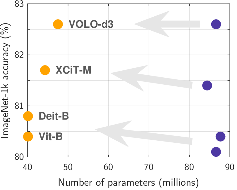
Figure 1: We redesign popular transformers models with an increased number of heads, using the theoretical insight that multi-head attention contributes to improving the conditioning of attention blocks. The benefits are so significant that we can reduce model depth while maintaining or improving accuracy, using about 50% fewer parameters.

Transformers [36] have become the dominant architecture across a wide range of fields, including natural language processing (NLP) [36, 6, 45, 43], computer vision [8, 4, 22, 34], and robotics [10, 24, 29]. At the heart of their success lies the attention mechanism, which dynamically assigns relevance scores to input elements, enabling the model to generate highly contextualized outputs. This ability allows transformers to capture complex dependencies in data more effectively than traditional architectures.

As transformers continue to scale, the prevailing belief is that heavy overparameterization is necessary for strong performance. A standard decoder-only transformer increases capacity through three primary means: (1) expanding the number of attention heads, (2) widening the feedforward layers, and (3) deepening the network by adding more layers. However, no well-established guidelines exist for balancing these components to achieve optimal performance. Extensive research has explored the role of width and depth in improving optimization for convolutional and feedforward networks [1, 3, 44, 16, 20, 21, 15]. For transformers however, our understanding of the trade-offs between width and depth remains incomplete [19, 18, 26, 30].

In this paper, we challenge the conventional approach to transformer design and ask whether these models are structured optimally. We introduce a theoretical principle that offers a new perspective on the role of multi-head attention, demonstrating that it inherently improves the conditioning of attention layers. This produces a matrix with a low condition number, which is the ratio of a matrix’s largest to smallest singular values. This quantifies its stability: a high condition number indicates ill-conditioning, which can hinder convergence of gradient-based optimization [25]. We theoretically show that using multiple heads lowers the condition number of attention layers and therefore facilitates the optimization of transformers.

We verify empirically that increasing the number of attention heads in transformers significantly improves the condition number of the attention block. We then use these insights to guide the design of transformer models, focusing on trade-offs with depth, one of the main choice in architecture design. We find empirically that transformers can often be redesigned with more attention heads and fewer layers while maintaining both optimization stability and accuracy. Since each layer corresponds to a large number of parameters, trading additional heads for fewer layers enables a substantial reduction in model size without compromising performance.

We validate our findings by modifying and re-training a range of existing models for vision and NLP tasks. We show that attention heads can be consistently traded for depth, resulting in more parameter-efficient architectures without sacrificing performance (see Fig. 1). While we lack a full theoretical explanation for this trade-off, our results raise important questions. Are transformers unnecessarily over-parameterized? Are other trade-offs possible by improving the conditioning of existing architectures? These results open multiple opportunities for future empirical and theoretical work.

Our contributions are summarized as follows.

1. A theoretical framework offering a new perspective on multi-head attention, indicating that one of its core functions is to better condition the attention block.

2. An empirical design principle for transformers derived from our theoretical insights, suggesting that model depth can be traded for additional heads to reduce parameter count without compromising accuracy.

3. A comprehensive empirical validation of downstream benefits for a variety of existing models on standard vision and NLP tasks: image classification with ImageNet-1k [32], language modeling with TinyStories [9] and GLUE benchmark [38], and long-context reasoning with the LRA benchmark [33].

2 Related Work

Efficient attention-based architectures.

Numerous approaches have been proposed to enhance the efficiency and effectiveness of transformers, particularly by reducing the computational complexity of the attention layer. DeiT (Data-Efficient Image Transformer) [34] improves training efficiency by leveraging distillation tokens, enabling strong performance with significantly fewer data requirements. XCiT (Cross-Covariance Image Transformer) [2] introduces a novel attention mechanism that operates on spatial feature cross-covariances, improving feature interactions while substantially reducing computational overhead. VOLO (Vision Outlooker) [42] incorporates outlook attention, which efficiently captures long-range dependencies, outperforming traditional vision transformers (ViTs) while maintaining computational efficiency. Nyströmformer [41] tackles the quadratic complexity of self-attention using a Nyström-based approximation, reducing it to near-linear time while preserving key attention properties. Other efficient transformer variants have further addressed attention-related bottlenecks. Linformer [39] approximates self-attention with low-rank projections, achieving linear complexity by compressing the sequence length dimension. Performer [5] employs kernelized attention with random feature projections, enabling scalable attention with linear time complexity. Reformer [17] utilizes locality-sensitive hashing to significantly reduce memory and computational costs, making attention efficient even for long sequences.

We take a different approach, exploring whether the inherent complexity of transformers can be reduced to create more compact models that maintain strong performance. Our insights on conditioning are orthogonal to the above methods and we demonstrate benefits on several of the aforementioned architectures (ViTs, Nyströmformers).

Network width and depth.

A vast literature has explored the roles of width and depth [23, 27, 35] and their interplay with gradient-based optimization. For example, Liu et al. [22] demonstrated that increasing the width of multi-layer perceptrons (MLPs) enhances the conditioning of their neural tangent kernel (NTK) [15], leading to more effective optimization. Arora et al. [3] showed that, in linear MLPs, depth serves as a preconditioner for stochastic gradient descent, improving optimization as depth increases. Similarly, Agarwal et al. [1] found that depth enhances the conditioning of non-linear MLPs, provided that activations are properly normalized, thereby facilitating better convergence with gradient-based algorithms.

The above studies underscore the importance of both width and depth in achieving good optimization for MLPs. A similar theoretical understanding for transformers is lacking [19, 18, 26, 30] and our work helps fill this gap. We also reveal a crucial role of the multi-head attention in the optimization of transformers and explore its empirical relationship with model depth.

3 Theoretical Findings

3.1 Preliminaries

Transformers.

We first briefly review the the transformer architecture [36, 8]. A transformer is composed of stacked layers, also known as “transformer blocks”. Each layer is formally represented as a mapping $\mathbf{T}:\mathbb{R}^{N\times D}\rightarrow\mathbb{R}^{N\times D}$ defined by the expression $\mathbf{T}(X)=\mathbf{F}(\mathbf{A}(X)+X)$. The component $\mathbf{F}$ denotes a feedforward multi-layer perceptron (MLP, typically with one hidden layer and a residual connection), and $\mathbf{A}$ represents the self-attention mechanism.

The self-attention mechanism $\mathbf{A}$ uses three learnable matrices, the query ($Q$), key ($K$), and value ($V$) matrices. Given an input sequence $X\in\mathbb{R}^{N\times D}$, the matrices are first applied as follows: $q\!=\!QX$, $k\!=\!KX$, $v\!=\!VX$, where $Q,K\in\mathbb{R}^{D\times d}$  and $V\in\mathbb{R}^{D\times M}$. These are then combined to produce the output of the self-attention head as follows: $\mathbf{A}(X):=\operatorname{\mathbf{softmax}}(\,q\,k^{T})\,v$, where the softmax is applied row-wise. In this paper, whenever we speak of an attention matrix we will mean the matrix $\operatorname{\mathbf{softmax}}(\,q\,k^{T})\,v$. Multiple parallel attention heads $\mathbf{A}_{i}$ are typically used ($1\leq i\leq h$), each of dimension $N\times\frac{D}{h}$. Their outputs are concatenated as $[\mathbf{A}_{1},\cdots,\mathbf{A}_{h}]$, which is then fed into the MLP. Additional normalizations and residual connections are often interleaved depending on the model’s specific details.

Condition number.

The condition number of a matrix is the ratio of its largest to smallest singular values. In gradient-based optimization of linear and non-linear systems, the condition number serves as a quantitative measure of how well the optimizer will converge. Lower values indicate a more stable and efficient convergence. Conversely, a matrix is said to be ill-conditioned if the condition number is high. Ill-conditioned matrices in non-linear systems lead to difficulties for gradient descent to converge [25].

Definition 3.1.

The condition number of a full-rank, $n\times m$ matrix $A$ is defined as $\kappa(A)\!:=\!\sigma_{1}(A)\;/\;\sigma_{k}(A)$, with the singular values $\sigma_{1}(A)\geq\dots\geq\sigma_{k}(A)$ and $k=\min(m,n)$.

Since $A$ is of full rank, all singular values are positive and the condition number is thus well defined. And since $\sigma_{1}(A)\geq\sigma_{k}(A)$, the condition number satisfies $\kappa(A)\geq 1$.

3.2 Main Theoretical Result

Our main finding states that multi-head attention has the implicit effect of conditioning the self-attention block within a transformer layer, which leads to attention matrices ($A_{i}$) with a low condition number. This in turn facilitates the optimization of transformers by gradient descent.

Theorem 3.2.

Let $\mathbf{A}_{i}\in\mathbb{R}^{N\times\frac{D}{h}}$ be i.i.d Gaussian random variables ($1\leq i\leq h$). We define the multi-head matrix block $\mathbf{A}=[\mathbf{A}_{1},\cdots,\mathbf{A}_{h}]$ of dimension $N\times D$ and assume $D>>N$. Then, the condition number

$$\kappa(\mathbf{A})\approx 1.$$ (1)

Moreover, if we fix the dimension of the attention heads $d>0$ such that $\mathbf{A}_{i}\in\mathbb{R}^{N\times d}$, we have:

$$\kappa(\mathbf{A})\rightarrow 1\text{ ~~as~~ }h\rightarrow\infty.$$ (2)

To prove Theorem 3.2 we will need the following lemma.

Lemma 3.3.

Let $X$ be a matrix in $\mathbb{R}^{m\times n}$ with $n>>m$ whose entries are i.i.d drawn from a Gaussian distribution. Then $X$ is full rank with probability 1.

The proof of Lemma 3.3 is given in Appendix A.

Proof of Theorem 3.2.

The proof will proceed by using some well known facts about random matrices, see [37] for proofs. Firstly given a random Gaussian matrix $X$ of full rank and size $m\times n$ with $n>>m$ we have that the minimum singular value, $\sigma_{m}(X)$, and maximum singular value of $X$, $\sigma_{1}(X)$, satisfy

$$\sigma_{m}(X)\approx\sqrt{n}-\sqrt{m}\text{ and }\sigma_{m}(X)\approx\sqrt{n}+\sqrt{m}.$$ (3)

We start by proving the first part of the theorem. Observe that, by assumption, the multi-head matrix

$$\mathbf{A}=[\mathbf{A}_{1},\cdots,\mathbf{A}_{h}]$$ (4)

has shape $N\times D$ where $D>>N$. Furthermore, since each $\mathbf{A}_{1}$ is drawn i.i.d. from a Gaussian distribution, we have from Lemma 3.3 that $\mathbf{A}$ has full rank which is $N$. Then, applying Eq. (3) we have that

$$\sigma_{N}(\mathbf{A})\approx\sqrt{D}-\sqrt{N}\text{ and }\sigma_{1}(\mathbf{A})\approx\sqrt{D}+\sqrt{N}.$$ (5)

By the definition of the condition number, we then find that

$$\kappa(\mathbf{A}):=\frac{\sigma_{1}(\mathbf{A})}{\sigma_{N}(\mathbf{A})}\approx\frac{\sqrt{D}+\sqrt{N}}{\sqrt{D}-\sqrt{N}}.$$ (6)

Since $D>>N$, we have $\frac{\sqrt{N}}{\sqrt{D}-\sqrt{N}}\approx 0$ and

$$\frac{\sqrt{D}}{\sqrt{D}-\sqrt{N}} =\frac{\sqrt{D}-\sqrt{N}}{\sqrt{D}-\sqrt{N}}+\frac{\sqrt{N}}{\sqrt{D}-\sqrt{N}}$$ (7)

$$\approx\frac{\sqrt{D}-\sqrt{N}}{\sqrt{D}-\sqrt{N}}$$ (8)

$$=1$$ (9)

This then implies that

$$\kappa(\mathbf{A}) \approx\frac{\sqrt{D}+\sqrt{N}}{\sqrt{D}-\sqrt{N}}$$ (10)

$$=\frac{\sqrt{D}}{\sqrt{D}-\sqrt{N}}+\frac{\sqrt{N}}{\sqrt{D}-\sqrt{N}}$$ (11)

$$\approx 1$$ (12)

which proves the first part of the theorem.

To prove the second part of the theorem, observe that if $h\rightarrow\infty$ then, using Eq. (3), the condition number is given by

$$\kappa(\mathbf{A})\approx\frac{\sqrt{dh}+\sqrt{N}}{\sqrt{dh}-\sqrt{N}}\rightarrow 1\text{ as }h\rightarrow\infty.\vskip-5.0pt$$ (13)

∎

The theorem highlights that, while an individual attention matrix $\mathbf{A}_{i}$ of dimension $N\times\frac{D}{h}$ may not be well-conditioned, the concatenation of multiple such matrices improves their overall condition number. This insight offers a new perspective on multi-head attention: it functions as an implicit conditioner, enhancing the conditioning of each attention block within a transformer.

Observation.

We observe that in Eq. 2 we could have also let $d$ go to infinity and the same proof shows that the matrix $\mathbf{A}$ would have condition number going to $1$. However, observe that, when $d$ is fixed, each attention head computes an $N\!\times\!d\,$ projection independently. With $h$ heads, these computations can be parallelized, allowing efficient scaling. In contrast, increasing $d$ while keeping $h$ fixed enlarges each head’s computation, leading to slower training due to reduced parallelism. Therefore in this paper, we will focus on lowering the condition number of $\mathbf{A}$ by increasing the number of heads.

3.3 Trading Depth for Heads

We demonstrated in Theorem 3.2 that additional heads improve the conditioning of an attention layer. We now examine how this can translate into tangible performance gains.

Conditioning in MLPs.

The existing literature provides theoretical support for improved performance of MLPs with better-conditioned weight matrices trained with gradient descent. Liu et al. [21] used the Neural Tangent Kernel (NTK) framework [15] to show that increasing network width reduces the NTK’s condition number, thereby enhancing convergence. As MLPs widen, their weight matrices enter the regime described in Theorem 3.2 where the condition number approaches $1$. By direct application of the chain rule, this implies that the improved conditioning of the weight matrices leads to a better-conditioned NTK. Complementary studies [1, 3] reveal that increasing depth also helps conditioning for gradient-based optimizers. Together, these results underscore the dual importance of both width and depth in the optimization of MLPs.

What about transformers?

Each transformer layer consists of a multi-head attention and an MLP. Transformers employ wide MLPs, typically 2$\times$ to 4$\times$ the dimension of token embeddings. They are thus likely to be well conditioned. We therefore focus on widening the attention block by increasing the number of heads. According to Theorem 3.2, we expect this to bring the condition number of each attention block towards $1$. We will verify empirically in Sec. 4 that this is indeed the case (Fig. 2).

Trading depth and width.

The literature discussed above suggests that depth and width have complementary roles for the optimization of neural models. We therefore hypothesize that increasing the number of attention heads could be matched with a reduction in depth while maintaining performance. The motivation stems from the fact that each layer uses a large amount of parameters, hence a reduction in depth quickly decreases the model size. In other words, additional attention heads could enable the design of compact transformers that perform comparably to deeper ones.

The experiments in Sec. 4 will extensively validate this hypothesis across a range of architectures and tasks. A theoretical explanation as to why reducing depth yields such strong performance is still incomplete. Our results open important questions for future work about optimal architecture design from both theoretical and empirical perspectives.

4 Experiments

We perform extensive experiments with a variety of transformer-based models. Our goals are (1) to empirically verify the prediction of Theorem 3.2 about improvements in conditioning and (2) to evaluate the downstream benefits on standard vision and NLP tasks: image classification with ImageNet-1k [32], language modeling with TinyStories [9], and long-context reasoning with the LRA benchmark [33].

4.1 Image Classification

We consider standard large vision transformers (ViTs) from the literature. We modify their architecture according to the findings from Sec. 3 and re-train them from scratch on ImageNet-1k [32]. Our approach enables reductions in parameter count by up to 30%–50% of existing models without compromising their accuracy. The explicit training details, implementation and hardware used for all experiments in this subsection can be found in Sec. B.1.

4.1.1 Standard ViTs

We use the ViT-Base (ViT-B) architecture [8], a popular model for image classification. The model processes an input image as non-overlapping patches of $16\!\times\!16$ pixels. They are linearly projected into token embeddings of dimension $768$ that serve as input to the transformer layers. ViT-B uses $12$ layers, each with $12$ attention heads of dimension $64$ ($12\times 64\!=\!768$, the initial token embedding size). Its MLPs use hidden layers of size $4\times 768\!=\!3,072$.

Validating the effects on conditioning.

To validate Theorem 3.2, we systematically vary the number of heads in a ViT-B and re-train the model on ImageNet-1k. We train each model to convergence i.e. for about 300 epochs. For each training run, every 50 epochs, we compute the condition number of each layer’s attention matrix and average them across layers. We examine the results in Fig. 2 and observe that the condition number decreases markedly as the number of heads increases, thus validating Theorem 3.2.

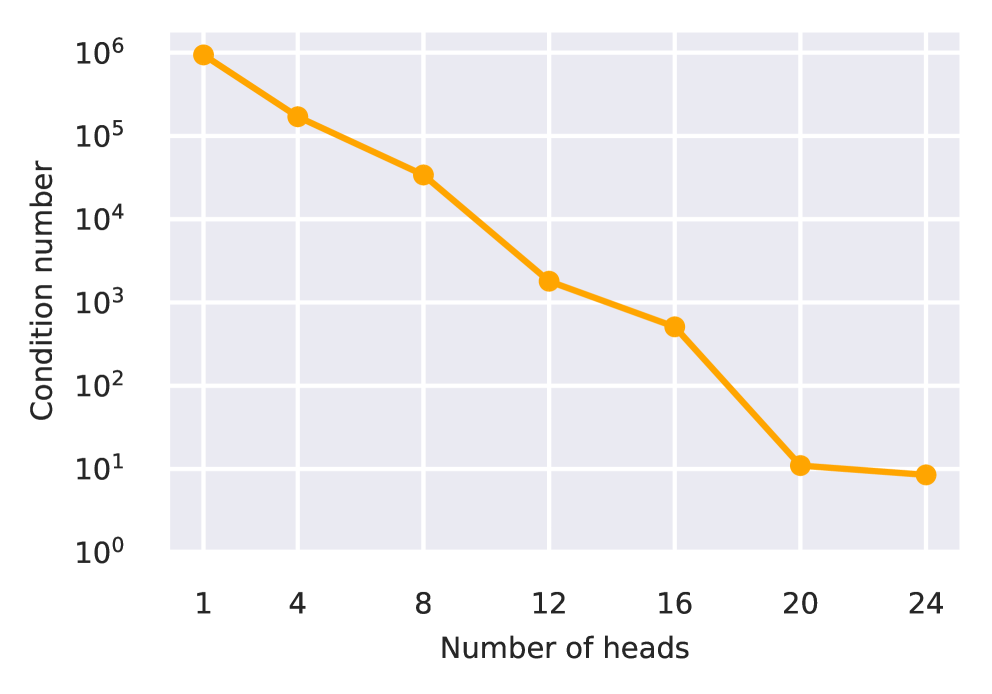
Figure 2: Empirical measurement of the condition number of the attention layers in ViT-Bs with different numbers of heads. The conditioning improves (lower number) with additional heads, following the predictions of Theorem 3.2.

12 Layers                             8 Layers

Figure 3: Accuracy on ImageNet-1k of variants of ViT-B with the original depth (12 layers, left) or reduced to 8 layers (right). Each point is annotated with the model’s total number of parameters (in millions). According to our predictions, the number of heads correlates with performance. Remarkably, our models with reduced depth (right) and $\geq$12 heads (green dots) all obtain a higher test accuracy with fewer parameters than the original model (dotted line).

12 Layers                             8 Layers

Figure 4: Similar experiments as Fig. 3, where each model is now a variant of ViT-B with a different MLP width (X axes, reported as a factor of the token-embedding size). According to our predictions, increasing the width of MLPs has a weaker effect than adding attention heads. The slight benefit observed with 12 layers (left) cannot compensate for a reduction of depth to 8 layers (right), unlike what was observed with additional heads in Fig. 3.

New model configurations.

We first fix the depth at $12$ layers as in the original model, and vary the number of heads from $2$ to $18$, keeping a constant head dimension of $64$. Following the discussion in Sec. 3.3, we then consider a reduced depth of $8$ layers, and vary again the number of heads from $2$ to $18$. We train each configuration on ImageNet-1k and measure the top-1% accuracy. Training uses the AdamW optimizer for $300$ epochs following standard strategy from prior work [32] (details in Appendix B).

The results in Fig. 3 (left) show a clear improvement in accuracy as the number of heads increases, including higher performance than the original model with $>$12 layers, at the cost of additional parameters. We then examine a model with a depth reduced from 12 to 8 layers (Fig. 3, right). The accuracy is again correlated with the number of heads. The smaller number of layers largely makes up for those in additional heads, and all configurations with $>$12 heads surpass the accuracy of the original one with a much smaller parameter count (61.2 – 67.4 M vs. 86.6 M).

MLP hidden-layer width:  ◼ 2$\times$   ⚫ 4$\times$ token embedding size

Figure 5: Additional variants of ViT-B with different numbers of layers and heads, and MLP width. Each model is annotated with its reduction in parameters. For 6–-8 layers, doubling the MLP width yields little benefit, indicating that the number of heads is more important.

⚫ Ours (more heads, fewer layers)    ⚫ Original
    

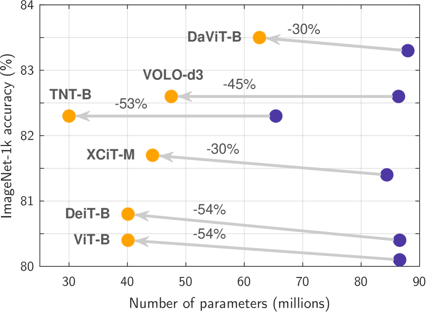
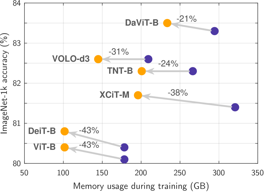
Figure 6: Other vision transformer architectures. We plot improvements in accuracy against reductions in parameter count (top) and memory usage during training (bottom). All models benefit significantly from our approach.

⚫ Ours (more heads, fewer layers)    ⚫ Original

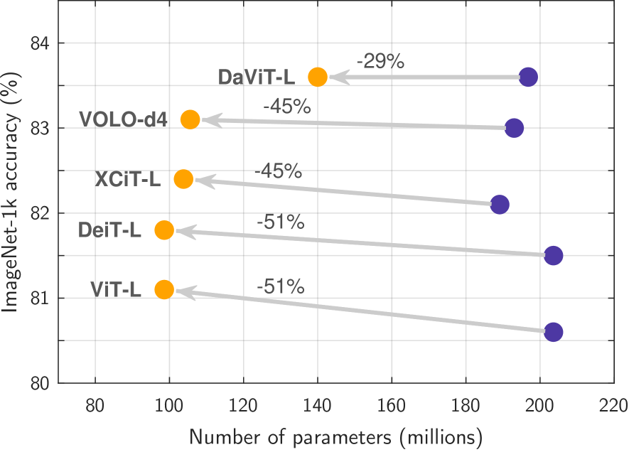
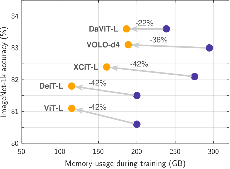
Figure 7: Large vision transformer architectures. We observe the same improvements in accuracy, parameter count, and memory usage as with other models.

MLP width.

We now consider variations of the hidden-layer size of the MLPs inside a ViT-B model, as an alternative strategy to affect the width of the model. The original model uses a size of $768\!\times\!4\,=\,3,072$, where 768 is the token embedding size and 4 is referred to as the “MLP ratio”. We train models with a ratio between 1 and 8. Fig. 4 shows a limited impact on accuracy that contrasts with the clear large effects of the number of heads from Fig. 3. This agrees with the hypothesis made in Sec. 3.3 that MLPs are likely to be already well-conditioned and do not benefit in this regard as much as attention blocks in transformers.

Best configurations.

We evaluate additional configurations with depths below $8$ in Fig. 5. We adjust the number of heads to match the accuracy of the original ViT-B ($\geq 80.1\%$). All configurations still use much fewer parameters than the original model with a better accuracy.

4.1.2 Other Vision Transformers

We apply our strategy to a variety of alternative transformer-based architectures in the 60–90 M parameter range: DeiT [34], XCiT [2], TNT [14], VOLO [42], and DaViT [7], all pretrained on ImageNet-1k. We report our best configurations in Fig. 6 . In all cases, reducing depth and increasing the number heads leads to models with similar or higher accuracy with substantial reductions in parameter count. This indicates that many models are unnecessarily oversized. This also corresponds to substantial reductions in memory during training (reported separately in Fig. 6).

Larger models.

We also evaluate models in the 180 – 200 M parameter range. Fig. 7 shows similar improvements in accuracy, parameter count, and memory usage.

4.2 Language Modeling

We evaluate our approach on two language models.

Crammed BERT.

We first consider the Crammed-BERT architecture [13]. trained on the Pile dataset [11] following Geiping and Goldstein [13]. We evaluate these models on the GLUE benchmark [38].

	MNLI	SST-2	STSB	RTE	QNLI	QQP	MRPC	CoLA	GLUE	Parameters	Memory
Crammed BERT (original)	83.8	92.3	86.3	55.1	90.1	87.3	85.0	48.9	78.6	$119$ M	$13.8$ GB
Crammed BERT (ours)	83.7	92.3	86.3	55.3	90.0	87.3	85.2	48.9	78.6	$84$ M ($-29\%$)	$10.3$ GB ($-25\%$)

Table 1: Comparison of a pretrained original Crammed BERT (16 layers, 12 heads per layer) with our leaner variant (10 layers, 24 heads) on the GLUE benchmark. For each task our learner variant achieves comparable performance with much less parameters.

We train several variants of Crammed BERT with different numbers of attention heads and layers. The original model uses 12 heads and 16 layers. As hypothesized, we find that increasing the number of heads leads to better performance, so much so that the depth can be reduced and still match the performance of the original model (see Tab. 1). In particular, we find that 24 attention heads and 10 layers produce a compact architecture that performs similarly on GLUE as the original model.

GPT-2.

We proceed similarly with a GPT-2 architecture trained on the TinyStories dataset [9]. As the original configuration, we use the 12-layer, 12-head model (89 M parameters) from Eldan and Li [9]. We then increase the number of heads to 16 while reducing the depth to 4 layers. As shown in Tab. 2, our variant outperforms the original one in validation loss. Moreover, it achieves these improvements with significantly fewer parameters and reduced memory usage during training.

	Val. loss	Parameters	Memory
GPT-2 (original)	2.47	$89$ M	$12.8$ GB
GPT-2 (ours)	2.41	$64$ M (-$28\%$)	$9.7$ GB (-$24\%$)

Table 2: GPT-2 models trained on the TinyStories dataset. We compare a baseline model with 12 layers and 12 attention heads [9] and our variant with 4 layers and 16 heads. We achieve superior performance at a much smaller size and memory usage.

4.3 LRA Benchmark with Nyströmformers

2 Layers                               1 Layer 

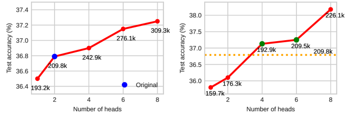
Figure 8: Accuracy on the ListOps task of the LRA benchmark with variants of the Nyströmformer. The original model from Xiong et al. [41] uses 2 layers (left) and we also evaluate models with a single layers (right). Each model is annotated with its total number of parameters. According to our predictions, the number of heads correlates with performance. Remarkably, our models with just 1 layer and $\geq$ 4 heads (green dots) all obtain a higher test accuracy with fewer parameters than the original model (dotted line).

2 Layers                               1 Layer 

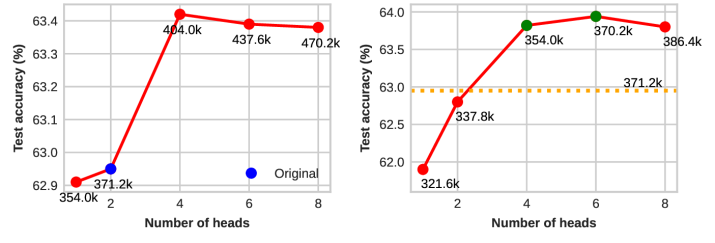
Figure 9: Accuracy on the text classification task of the LRA benchmark with variants of the Nyströmformer. The original model from Xiong et al. [41] uses 2 layers (left) and we also evaluate models with a single layers (right). Each model is annotated with its total number of parameters. According to our predictions, the number of heads correlates with performance. Remarkably, our models with just 1 layer and $\geq$ 4 heads (green dots) all obtain a higher test accuracy with fewer parameters than the original model (dotted line).

We evaluate our approach on Nyströmformers [41], a transformer-like architecture that uses an approximation of the self-attention with better computational complexity. Our objective is to evaluate the relevance of our findings to an architecture that slightly departs from the original transformer architecture of Vaswani [36]. Nyströmformers are well suited to long sequences and we therefore evaluate them on the Long-Range Arena (LRA) benchmark [33].

Our base model follows the original paper [41] and uses 2 layers and 2 attention heads per layer. We also train variants with 2-8 heads and 1-2 layers. The results on the ListOps task (see Fig. 8) and the Text classification task (see Fig. 9) show that additional heads increase the accuracy. This allows reducing the depth to a single layer while improving its accuracy. These results hold across other tasks of the LRA benchmark (see Tab. 3).

ListOps
(Depth, heads)	Top-1% Acc.	Parameters
(2, 2)	36.79	209.8k
(1,4)	37.13	192.9k	(-9%)
Text Classification
(Depth, heads)	Top-1% Acc.	Parameters
(2, 2)	62.95	371.2k
(1,4)	63.82	354.0k	(-5%)
Document Retrieval
(Depth, heads)	Top-1% Acc.	Parameters
(2, 2)	79.3	394.8k
(1,4)	79.5	394.8k	(same)
Image Classification
(Depth, heads)	Top-1% Acc.	Parameters
(2, 2)	37.2	191.2k
(1,4)	38.2	191.2k	(same)
Pathfinder
(Depth, heads)	Top-1% Acc.	Parameters
(2, 2)	69.8	190.2k
(1,4)	69.9	190.2k	(same)

Table 3: Evaluation of variants of the Nyströmformer [41] on different datasets of the Long-Range Arena (LRA) benchmark [33]. We compare the original model (2 layers, 2 heads) with our variant (1 layer, 4 heads). On every task, it outperforms the original model with the same number or slightly fewer parameters.

5 Conclusions

In this work, we reexamined the role of multi-head attention in transformers. Our theoretical analysis revealed that increasing the number of heads improves the conditioning of the attention matrices, a finding we confirmed empirically on vision transformers. Building on previous studies of MLP conditioning, we hypothesized that an increase of the number of heads could reduce the depth required to achieve high performance. We tested this idea on tasks including image classification, language generation, and long sequence modeling, and found that leaner, shallower architectures with more attention heads perform comparably to their deeper counterparts. These results suggest a promising avenue for designing more efficient transformers without sacrificing performance.

Limitations and Open Questions

• We empirically demonstrated that depth can be traded off for more attention heads while maintaining performance. However, a theoretical explanation for this balance is still missing. Can we quantitatively predict the trade-offs of specific architectural variations?

• Our main theorem shows that increasing the number of heads improves the condition number of attention layers. The subsequent effect on task accuracy then rests on empirical results. How exactly does this form of conditioning impact training dynamics and downstream performance?

• Are there other architectural interventions that could achieve similar effects to the additional attention heads? Alternative methods for conditioning the attention layers could further improve the efficiency of transformers.

• Our resources allowed experiments on models with up to $\sim$200M parameters. Do the observed benefits persist at larger scales such as in $\sim$1B-parameter models?

Supplementary Material / Appendix

Appendix A Theoretical Framework

In Sec. 3 we used Lemma 3.3 in the proof of our main Theorem 3.2. We give the proof of the lemma.

Proof of Lemma 3.3.

We first note that any measure defined via a Gaussian or probability distribution is absolutely continuous with respect to the Lebesgue measure [31]. Meaning they have the same sets of measure zero as the Lebesgue measure.

Write $X=[X_{1},\ldots,X_{n}]$ where each $X_{i}\in\mathbb{R}^{m}$ for $1\leq i\leq n$. We first prove the case that that $\{X_{1},\ldots,X_{n}\}$ are vectors of unit length. Since the vectors were drawn independently, we can first assume we drew $X_{1}$. The probability that this is the zero vector is $0$ w.r.t the Lebesgue measure on the closed unit ball $B_{N}(0)$ about the origin in $\mathbb{R}^{N}$ and hence any other measure absolutely continuous to it. Then draw $X_{2}$ and note that the probability that $X_{2}$ lies in $span\{X_{1}\}\cap B_{N}(0)$ is also $0$ since $span\{X_{1}\}\cap B_{N}(0)$ forms a set of $0$ Lebesgue measure in $B_{N}(0)$. Continuing in this way we find that $\{X_{1},\ldots,X_{n}\}$ will be linearly independent with probability $1$ implying that the matrix $X$ has full rank.

For the general case where $\{X_{1},\ldots,X_{n}\}$ are not drawn to have unit length i.e. drawn on the sphere in $\mathbb{R}^{N}$, we simply note that we can draw each one and then divide by its norm producing one of unit length. Since normalizing by the norm doesn’t affect linear independence we get by the above case that $\{X_{1},\ldots,X_{n}\}$ must be linearly independent with probability $1$. ∎

Appendix B Experimental Details

B.1 Vision transformers on ImageNet-1k

Detailed results for vision transformers

In Sec. 4.1.2, we demonstrated that several base vision transformers from the literature, ranging from 60 to 90 million parameters, benefit from our approach of increasing the number of heads in each attention layer while reducing the overall depth. In every instance, our configuration performed on par with or better than the original architecture while significantly lowering both parameter count and memory usage (see Fig. 6). The detailed configurations are provided in Tab. 4.

We also showed that our methodology could be applied to larger vision transformers with roughly 180-200 million parameters (Fig. 7). The configurations for these larger ViTs are given in Tab. 5.

ViT-B on ImageNet-1k
(Depth, Heads)	MLP dim.	Top-1% Acc.	Top-5% Acc.	Params. (millions)	Memory (GB)
(12, 12)	3072	80.1	94.2	86.6	178.4
(7,16)	1536	80.4	94.9	40.1	101.6
DeiT-B on ImageNet-1k
(Depth, Heads)	MLP dim.	Top-1% Acc.	Top-5% Acc.	Params. (millions)	Memory (GB)
(12, 12)	3072	80.4	95.1	86.6	178.4
(7,16)	1536	80.8	95.3	40.1	101.6 $\color[rgb]{0,1,0}\downarrow$
XCiT-Medium on ImageNet-1k
(Depth, Heads)	MLP dim.	Top-1% Acc.	Top-5% Acc.	Params. (millions)	Memory (GB)
(24, 8)	2048	81.4	95.5	84.4	320.8
(12,16)	2048	81.7	95.6	59.0	196
TNT-B on ImageNet-1k
(Depth, Heads)	MLP dim.	Top-1% Acc.	Top-5% Acc.	Params. (millions)	Memory (GB)
(12, 10)	2560	82.3	95.7	65.4	266.4
(8,16)	2560	82.3	95.8	30.9	200.8
VOLO-d3 on ImageNet-1k
(Depth, Heads)	MLP dim.	Top-1% Acc.	Top-5% Acc.	Params. (millions)	Memory (GB)
([8, 8, 16, 4], [8, 16, 16, 16])	(1024, 2048, 2048, 2048)	82.6	95.6	86	209.2
([4, 4, 8, 2], [16, 32, 32, 32])	(768, 1536, 1536, 1536)	82.6	95.7	47.5	144.8
DaViT-B on ImageNet-1k
(Depth, Heads)	MLP dim.	Top-1% Acc.	Top-5% Acc.	Params. (millions)	Memory (GB)
([1,1,9,1], [4, 8, 16, 32])	(512, 1024, 2048, 4096)	83.3	96.0	88.0	294.4
([1, 1, 5, 1], [4, 8, 32, 32])	(512, 1024, 2048, 4096)	83.5	96.1	62.0	233.6

Table 4: Detailed configurations for a variety of base vision transformers from the literature. Increasing the heads and reducing depth (green) we obtain several transformers that outperform their original counterparts (red) with less parameters and less memory for training.

ViT-L on ImageNet-1k
(Depth, Heads)	MLP dim.	Top-1% Acc.	Top-5% Acc.	Params. (millions)	Memory (GB)
(24, 16)	4096	80.6	94.4	203.6	200.0
(8,30)	2048	81.1	95.1	98.6	115.2
DeiT-L on ImageNet-1k
(Depth, Heads)	MLP dim.	Top-1% Acc.	Top-5% Acc.	Params. (millions)	Memory (GB)
(24, 16)	4096	81.5	95.3	203.6	200.0
(8,30)	2048	81.8	95.4	98.6	115.2 $\color[rgb]{0,1,0}\downarrow$
XCiT-L on ImageNet-1k
(Depth, Heads)	MLP dim.	Top-1% Acc.	Top-5% Acc.	Params. (millions)	Memory (GB)
(24, 16)	3072	82.1	95.9	189.1	275.2
(12,24)	3072	82.4	95.9	103.8	160.8
VOLO-d4 on ImageNet-1k
(Depth, Heads)	MLP dim.	Top-1% Acc.	Top-5% Acc.	Params. (millions)	Memory (GB)
([8, 8, 16, 4], [12, 16, 16, 16])	(1536, 3072, 3072, 3072)	83.0	96.1	193.0	294.4
([4, 4, 8, 2], [24, 32, 32, 32])	(768, 1536, 1536, 1536)	83.1	96.2	105.6	188.8
DaViT-L on ImageNet-1k
(Depth, Heads)	MLP dim.	Top-1% Acc.	Top-5% Acc.	Params. (millions)	Memory (GB)
([1,1,9,1], [6, 12, 24, 48])	(768, 1536, 3072, 6144)	83.6	96.5	196.8	238.4
([1, 1, 5, 1], [6, 12, 48, 48])	(768, 1536, 3072, 6144)	83.6	96.6	140.0	186.4

Table 5: Detailed configurations for a variety of large vision transformers from the literature. Increasing the heads and reducing depth (green) we obtain several transformers that outperform their original counterparts (red) with less parameters and less memory for training.

Hardware and implementation.

All models were trained on 8 Nvidia A100 GPUs using the code base from huggingface: https://github.com/huggingface/pytorch-image-models. Note that we couldn’t find an implementation of a TNT large architecture in this code base and that is why we did not have TNT large in our analysis for large vision transformers. The training of each vision transformer architecture we considered follows [32] with explicit hyperparameter choices given in Tab. 6.

Hyperparameter	Value
Batch size	1024 for base and 512 for large
Number of epochs	300
Learning rate	3.00e-03
Optimizer	AdamW
Weight decay	0.3
Label smoothing	0.1
Number of warm-up epochs	20
Warmup learning rate	1.00e-05
Mixup	0.8
Cutmix	1
Drop path	0.1
RandAug	9, 0.5

Table 6: Hyperparameter settings for all vision transformer models.

B.2 Language Models

Hardware and implementation.

Both the Crammed BERT and GPT-2 models from Sec. 4.2 were trained on one Nvidia A6000 GPU. The implementation, training and hyperparameters of the Crammed BERT model followed the original GitHub repo [12]. The GPT-2 models were trained following the paper [9] and the github repo [28].

B.3 Nyströmformer

Hardware and implementation.

The Nyströmformer experiments carried out in Sec. 4.3 were done on one Nvidia A6000 GPU. The implementation followed the original paper [41] and its GitHub repo [40].

References

- Agarwal et al. [2021] Naman Agarwal, Pranjal Awasthi, and Satyen Kale. A deep conditioning treatment of neural networks. In Algorithmic Learning Theory, pages 249–305. PMLR, 2021.
- Ali et al. [2021] Alaaeldin Ali, Hugo Touvron, Mathilde Caron, Piotr Bojanowski, Matthijs Douze, Armand Joulin, Ivan Laptev, Natalia Neverova, Gabriel Synnaeve, Jakob Verbeek, et al. Xcit: Cross-covariance image transformers. Advances in neural information processing systems, 34:20014–20027, 2021.
- Arora et al. [2018] Sanjeev Arora, Nadav Cohen, and Elad Hazan. On the optimization of deep networks: Implicit acceleration by overparameterization. In International conference on machine learning, pages 244–253. PMLR, 2018.
- Carion et al. [2020] Nicolas Carion, Francisco Massa, Gabriel Synnaeve, Nicolas Usunier, Alexander Kirillov, and Sergey Zagoruyko. End-to-end object detection with transformers. In European conference on computer vision, pages 213–229. Springer, 2020.
- Choromanski et al. [2021] Krzysztof Choromanski, Valerii Likhosherstov, David Dohan, Xingyou Song, Alex Gane, Tamas Sarlos, Peter Hawkins, Jared Davis, Afroz Mohiuddin, Lukasz Kaiser, et al. Rethinking attention with performers. In International Conference on Learning Representations (ICLR), 2021.
- Devlin et al. [2018] Jacob Devlin, Ming-Wei Chang, Kenton Lee, and Kristina Toutanova. Bert: Pre-training of deep bidirectional transformers for language understanding. arXiv preprint arXiv:1810.04805, 2018.
- Ding et al. [2022] Mingyu Ding, Bin Xiao, Noel Codella, Ping Luo, Jingdong Wang, and Lu Yuan. Davit: Dual attention vision transformers. In European conference on computer vision, pages 74–92. Springer, 2022.
- Dosovitskiy et al. [2020] Alexey Dosovitskiy, Lucas Beyer, Alexander Kolesnikov, Dirk Weissenborn, Xiaohua Zhai, Thomas Unterthiner, Mostafa Dehghani, Matthias Minderer, Georg Heigold, Sylvain Gelly, et al. An image is worth 16x16 words: Transformers for image recognition at scale. arXiv preprint arXiv:2010.11929, 2020.
- Eldan and Li [2023] Ronen Eldan and Yuanzhi Li. Tinystories: How small can language models be and still speak coherent english? arXiv preprint arXiv:2305.07759, 2023.
- Fu et al. [2024] Daocheng Fu, Xin Li, Licheng Wen, Min Dou, Pinlong Cai, Botian Shi, and Yu Qiao. Drive like a human: Rethinking autonomous driving with large language models. In Proceedings of the IEEE/CVF Winter Conference on Applications of Computer Vision, pages 910–919, 2024.
- Gao et al. [2021] Leo Gao, Stella Biderman, Sid Black, Laurence Golding, Travis Hoppe, Charles Foster, Jason Phang, Horace He, Aadi Thite, Eric Nabeshima, et al. The pile: An 800gb dataset of diverse text for language modeling. arXiv preprint arXiv:2101.00027, 2021.
- Geiping [2023] Jonas Geiping. Cramming. https://github.com/JonasGeiping/cramming, 2023.
- Geiping and Goldstein [2023] Jonas Geiping and Tom Goldstein. Cramming: Training a language model on a single gpu in one day. In International Conference on Machine Learning, pages 11117–11143. PMLR, 2023.
- Han et al. [2021] Kai Han, An Xiao, Enhua Wu, Jianyuan Guo, Chunjing Xu, and Yunhe Wang. Transformer in transformer. Advances in neural information processing systems, 34:15908–15919, 2021.
- Jacot et al. [2018] Arthur Jacot, Franck Gabriel, and Clément Hongler. Neural tangent kernel: Convergence and generalization in neural networks. Advances in neural information processing systems, 31, 2018.
- Kabkab et al. [2016] Maya Kabkab, Emily Hand, and Rama Chellappa. On the size of convolutional neural networks and generalization performance. In 2016 23rd International Conference on Pattern Recognition (ICPR), pages 3572–3577. IEEE, 2016.
- Kitaev et al. [2020] Nikita Kitaev, Łukasz Kaiser, and Anselm Levskaya. Reformer: The efficient transformer. In International Conference on Learning Representations (ICLR), 2020.
- Levine et al. [2020a] Yoav Levine, Noam Wies, Or Sharir, Hofit Bata, and Amnon Shashua. The depth-to-width interplay in self-attention. arXiv preprint arXiv:2006.12467, 2020a.
- Levine et al. [2020b] Yoav Levine, Noam Wies, Or Sharir, Hofit Bata, and Amnon Shashua. Limits to depth efficiencies of self-attention. NeurIPS, 33:22640–22651, 2020b.
- Li et al. [2018] Xingguo Li, Junwei Lu, Zhaoran Wang, Jarvis Haupt, and Tuo Zhao. On tighter generalization bound for deep neural networks: Cnns, resnets, and beyond. arXiv preprint arXiv:1806.05159, 2018.
- Liu et al. [2022] Chaoyue Liu, Libin Zhu, and Mikhail Belkin. Loss landscapes and optimization in over-parameterized non-linear systems and neural networks. Applied and Computational Harmonic Analysis, 59:85–116, 2022.
- Liu et al. [2021] Ze Liu, Yutong Lin, Yue Cao, Han Hu, Yixuan Wei, Zheng Zhang, Stephen Lin, and Baining Guo. Swin transformer: Hierarchical vision transformer using shifted windows. In Proceedings of the IEEE/CVF international conference on computer vision, pages 10012–10022, 2021.
- Lu et al. [2017] Zhou Lu, Hongming Pu, Feicheng Wang, Zhiqiang Hu, and Liwei Wang. The expressive power of neural networks: A view from the width. Advances in neural information processing systems, 30, 2017.
- Maiti et al. [2023] Abhisek Maiti, Sander Oude Elberink, and George Vosselman. Transfusion: Multi-modal fusion network for semantic segmentation. In Proceedings of the IEEE/CVF Conference on Computer Vision and Pattern Recognition, pages 6536–6546, 2023.
- Nocedal and Wright [1999] Jorge Nocedal and Stephen J Wright. Numerical optimization. Springer, 1999.
- Petty et al. [2023] Jackson Petty, Sjoerd van Steenkiste, Fei Sha, Ishita Dasgupta, Dan Garrette, and Tal Linzen. The impact of depth and width on transformer language model generalization. openreview, 2023.
- Poole et al. [2016] Ben Poole, Subhaneil Lahiri, Maithra Raghu, Jascha Sohl-Dickstein, and Surya Ganguli. Exponential expressivity in deep neural networks through transient chaos. Advances in neural information processing systems, 29, 2016.
- [28] Praveen Raja. Tiny-stories-gpt. https://github.com/PraveenRaja42/Tiny-Stories-GPT.
- Salzmann et al. [2020] Tim Salzmann, Boris Ivanovic, Punarjay Chakravarty, and Marco Pavone. Trajectron++: Multi-agent generative trajectory forecasting with heterogeneous data for control. arXiv preprint arXiv:2001.03093, 2, 2020.
- Sanford et al. [2023] Clayton Sanford, Daniel J Hsu, and Matus Telgarsky. Representational strengths and limitations of transformers. NeurIPS, 36:36677–36707, 2023.
- Stein and Shakarchi [2009] Elias M Stein and Rami Shakarchi. Real analysis: measure theory, integration, and Hilbert spaces. Princeton University Press, 2009.
- Steiner et al. [2021] Andreas Steiner, Alexander Kolesnikov, Xiaohua Zhai, Ross Wightman, Jakob Uszkoreit, and Lucas Beyer. How to train your vit? data, augmentation, and regularization in vision transformers. arXiv preprint arXiv:2106.10270, 2021.
- Tay et al. [2021] Yi Tay, Mostafa Dehghani, Samira Abnar, Yikang Shen, Dara Bahri, Philip Pham, Jinfeng Rao, Julian Heinrich, Dai Hua, and Donald Metzler. Long range arena: A benchmark for efficient transformers. arXiv preprint arXiv:2011.04006, 2021.
- Touvron et al. [2021] Hugo Touvron, Matthieu Cord, Matthijs Douze, Francisco Massa, Alexandre Sablayrolles, and Hervé Jégou. Training data-efficient image transformers & distillation through attention. In International conference on machine learning, pages 10347–10357. PMLR, 2021.
- Vardi et al. [2022] Gal Vardi, Gilad Yehudai, and Ohad Shamir. Width is less important than depth in relu neural networks. In Conference on learning theory, pages 1249–1281. PMLR, 2022.
- Vaswani [2017] A Vaswani. Attention is all you need. Advances in Neural Information Processing Systems, 2017.
- Vershynin [2018] Roman Vershynin. High-dimensional probability: An introduction with applications in data science. Cambridge university press, 2018.
- Wang et al. [2018] Alex Wang, Amanpreet Singh, Julian Michael, Felix Hill, Omer Levy, and Samuel R Bowman. Glue: A multi-task benchmark and analysis platform for natural language understanding. arXiv preprint arXiv:1804.07461, 2018.
- Wang et al. [2020] Sinong Wang, Belinda Z Li, Madian Khabsa, Han Fang, and Hao Ma. Linformer: Self-attention with linear complexity. In Advances in Neural Information Processing Systems (NeurIPS), 2020.
- Xiong et al. [2021a] Yunyang Xiong, Zhanpeng Zeng, Rudrasis Chakraborty, Fei Tan, Glenn Fung, Vikas Singh, Xiaodong Yuan, Sungsoo Ahn Wang, Dimitris Papailiopoulos, and Katerina Fragkiadaki. Github repository, 2021a.
- Xiong et al. [2021b] Yunyang Xiong, Zhanpeng Zeng, Rudrasis Chakraborty, Mingxing Tan, Glenn Fung, Yin Li, and Vikas Singh. Nyströmformer: A nyström-based algorithm for approximating self-attention. Proceedings of the AAAI Conference on Artificial Intelligence, 2021b.
- Yuan et al. [2022] Li Yuan, Qibin Hou, Zihang Jiang, Jiashi Feng, and Shuicheng Yan. Volo: Vision outlooker for visual recognition. IEEE transactions on pattern analysis and machine intelligence, 45(5):6575–6586, 2022.
- Zhen et al. [2022] Q Zhen, W Sun, H Deng, D Li, Y Wei, B Lv, J Yan, L Kong, and Y Zhong. cosformer: rethinking softmax in attention. In International Conference on Learning Representations, 2022.
- Zhou and Feng [2018] Pan Zhou and Jiashi Feng. Understanding generalization and optimization performance of deep cnns. In International Conference on Machine Learning, pages 5960–5969. PMLR, 2018.
- Zhuang et al. [2021] Liu Zhuang, Lin Wayne, Shi Ya, and Zhao Jun. A robustly optimized bert pre-training approach with post-training. In Proceedings of the 20th chinese national conference on computational linguistics, pages 1218–1227, 2021.