Causal inference with dyadic data in randomized experiments

Abstract

Estimating the treatment effect within network structures is a key focus in online controlled experiments, particularly for social media platforms. We investigate a scenario where the unit-level outcome of interest comprises a series of dyadic outcomes, which is pervasive in many social network sources, spanning from microscale point-to-point messaging to macroscale international trades. Dyadic outcomes are of particular interest in online controlled experiments, capturing pairwise interactions as basic units for analysis. The dyadic nature of the data induces interference, as treatment assigned to one unit may affect outcomes involving connected pairs. We propose a novel design-based causal inference framework for dyadic outcomes in randomized experiments, develop estimators of the global average causal effect, and establish their asymptotic properties under different randomization designs. We prove the central limit theorem for the estimators and propose variance estimators to quantify the estimation uncertainty. The advantages of integrating dyadic data in randomized experiments are manifested in a variety of numerical experiments, especially in correcting interference bias. We implement our proposed method in a large-scale experiment on WeChat Channels, assessing the impact of a recommendation algorithm on users’ interaction metrics.

Keywords: Dyadic data; interference; online controlled experiment; social network.

1 Introduction

A randomized experiment is a study design in which participants are randomly assigned to different treatment groups to ensure reliable results. This methodology is widely adopted in online randomized controlled experiments (A/B testing), where it helps accurately assess the impact of various interventions on basic functional tests, user experiences, and other facets of digital platforms (Gupta et al.,, 2019; Kohavi et al.,, 2020). Thousands of large-scale online controlled experiments are conducted daily on major experimentation platforms. A key characteristic of such experiments in social networks is that an individual’s treatment may influence other users’ outcomes, which is referred to as interference. Interference dramatically increases the complexity of potential outcomes and possibly undermines the validity of causal inference because the stable unit treatment value assumption (SUTVA, Rubin,, 1980) no longer holds. It is crucial in problems involving social networks and is prevalent in various applications, such as communication and sharing behaviour among individuals mediated by a complex social network, and the spread of an infectious disease through a network of human interactions. For example, interference occurs when treatments influence outcomes through pairwise interactions, as exemplified by features like content sharing, collaborative tools, voice over internet protocol (VoIP) services, and matching games that necessitate mutual access (Karrer et al.,, 2021; Weng et al.,, 2024). In these scenarios, traditional unit-level randomization and corresponding estimators risk yielding biased feature value assessments due to interference effects.

Researchers have made significant progress in causal inference with interference, including various types of causal estimands (Hudgens and Halloran,, 2008; VanderWeele and Tchetgen,, 2011; Hu et al.,, 2022), models for interference mechanisms, and methods for identification and estimation (Eckles et al.,, 2016; Aronow and Samii,, 2017; Liu et al.,, 2016; Bhattacharya et al.,, 2020; Tchetgen Tchetgen et al.,, 2021; Leung,, 2022; Li and Wager,, 2022; Ogburn et al.,, 2024, 2020). Exposure mappings are proposed to fully or approximately describe the interference patterns and reduce the complexity of potential outcomes (Manski,, 2013; Aronow and Samii,, 2017; Chin,, 2019), which sometimes may not be available in real-world studies. For example, Sävje, (2024) quantified the potential influence of misspecified exposure mappings. In the context of randomized experiments with network interference, researchers also propose some methods to handle complicated interference at the design stage, such as cluster randomizations (Ugander et al.,, 2013; Ugander and Yin,, 2023), ego-cluster experiments (Saint-Jacques et al.,, 2019), or staggered rollout experiments (Cortez-Rodriguez et al.,, 2022; Han et al.,, 2023). In addition, there are other types of interference beyond network interference, such as carryover effects (Bojinov and Shephard,, 2019; Han et al.,, 2024) and peer effects (Goldsmith-Pinkham and Imbens,, 2013; Egami and Tchetgen Tchetgen,, 2024; Luo et al.,, 2025). This expanding corpus of research highlights the importance of addressing interference for reliable causal inference.

The previous proposals for handling interference in social networks have mainly focused on the analysis of unit-level data. However, dyadic data that capture interactions and relationships between pairs of units are becoming increasingly popular due to the proliferation of social media, which offer new opportunities for causal inference with interference. For example, some traditional unit-level outcomes, such as the number of received messages of a user, can be disaggregated into dyadic data recording the number of messages sent within each pair of users. The use of dyad-level information provides researchers with valuable insight into the complex interactions and intricate dynamics of units, thus improving the accuracy of policy decisions. Beyond social networks, the analysis of dyadic data is also appealing in various scientific fields, including cross-border equity flows (Portes and Rey,, 2005), international trade relations (Carlson et al.,, 2024), hunter-gatherer behaviours (Apicella et al.,, 2012), and network analysis in public health (Luke and Harris,, 2007).

In contrast to the vast literature on causal inference with unit-level outcomes, the research on causal inference with dyadic data is relatively sparse. Fafchamps and Gubert, (2007) studied the identification issues in dyadic data regression and developed a dyadic-robust variance estimator as an extension of the spatial heteroskedasticity and autocorrelation consistent (HAC) estimator. The dyadic-robust variance estimator has been successfully applied in the analysis of trade data by Cameron and Miller, (2014). Aronow et al., (2015) proposed a sandwich-type robust variance estimator for linear regression to account for complex clustering structure in dyadic data. Tabord-Meehan, (2019) established the statistical inference for dyadic robust $t$-statistics under more general conditions and asymptotic regimes. Canen and Sugiura, (2024) provided an alternative linear dyadic regression model that explicitly accounts for dependence across indirectly linked dyads. For nonparametric dyadic regression, Graham et al., (2021) presented the minimax lower bound of the mean regression function for dyadic data and provided a dyadic analogue of the familiar Nadaraya-Watson kernel regression estimator. Recently, Graham et al., (2024); Chiang and Tan, (2023); Cattaneo et al., (2024) studied kernel density estimation for dyadic data. These previous proposals have focused on the estimation and inference in dyadic regression or correlation rather than engaging deeply with the causal aspects of dyadic data.

Several previous proposals are closely related to our work. D’Amour and Airoldi, (2019) considered causal inference with dyadic data where the treatment is implemented on the dyad level. However, we primarily focus on the conventional randomized experiment setting where the treatment is assigned at the unit level. Bajari et al., (2023) considered dyadic outcomes in a bipartite setting, particularly in bipartite marketplaces, and designed a novel multiple randomization experimental design for buyer-seller pairs. They primarily focused on the dyadic outcomes defined on two populations, e.g., user-seller pairs. In the setting we consider, dyadic outcomes are defined within the same population, e.g., user-user pairs. Weng et al., (2024) investigated experimental design problems in one-sided matching platforms such as those in the online gaming industry and anonymous social networks by constructing a stochastic market model. Shi and Ding, (2024) established a central limit theorem for dyadic assignment procedures and developed hypothesis testing methods for correlation coefficients of dyadic outcomes.

In this paper, we focus on the global average treatment effect. We establish a design-based causal inference framework for randomized experiments with dyadic data, without invoking the linear model. Our primary contributions include introducing the dyadic interference problems, formalising the inference framework for dyadic data, and providing estimators with theoretical groundings. Specifically, in Section 2, we formalise randomized experiments with dyadic outcomes and develop unbiased estimators of the global average treatment effect under different randomization designs. In contrast, we show that a class of conventional estimators based on unit-level outcomes is in general, biased under the dyadic interference setting. In Section 3, we provide a comprehensive analysis of the proposed estimators and establish their theoretical properties. In Section 4, we discuss the confidence statement for the estimators proposed under Bernoulli randomization and complete randomization, including a class of variance estimators. In Sections 5, we illustrate the proposed methods with numerical simulations. In Section 6, we apply the proposed methods to analyse an experiment in WeChat that aims to promote interactions among users with a new recommendation algorithm.

2 Dyadic interference

Although most of the existing causal inference literature focused on unit-level outcomes, in some situations, the unit-level outcomes can be disaggregated into interactions between units. For example, the total volume of messages received by a user can be decomposed into message counts from individual contacts. Similarly, a user’s total call duration within a given week can be disaggregated into the contributions of each connected peer. Consider a finite population of $n$ units. We introduce the dyadic outcome $Y_{ij}$ to encode some pairwise interaction between units $i,j\in\{1,\dots,n\}$. The dyadic outcome can be an indicator of a binary, count-valued, or continuous-valued variable recording the observed interactions. The interaction can be either directed, where $Y_{ij}\neq Y_{ji}$, e.g., number of messages sent and received, or undirected, where $Y_{ij}=Y_{ji}$, e.g., the duration time of VoIP. Although some unit-level outcomes $Y_{ii}$ may exist in practice, we primarily focused on the dyadic outcomes $Y_{ij}$ with $i\neq j$ in the main text, and leave the discussions about the use of $Y_{ii}$ to Section 7.

Let $\bm{Z}=(Z_{1},Z_{2},\dots,Z_{n})\in\{0,1\}^{n}$ denote a vector of binary treatments assigned to the units, where $Z_{i}=1$ if unit $i$ receives the treatment and $Z_{i}=0$ if unit $i$ receives the control. In a randomized experiment, the treatment vector $\bm{Z}=\bm{z}$ is assigned according to a predetermined distribution $\operatorname{pr}(\bm{z})$. Although it is possible to do dyad-level randomization, i.e., assigning each pair of units to either treatment or control during each interaction, this approach may lead to an inconsistent user experience. Specifically, a given user may simultaneously experience both treatment and control conditions during interactions with distinct peers, thereby introducing estimation bias due to potential inconsistencies in user behaviour across differing experimental exposures.

We define the upstream and downstream neighbor sets for unit $i$ based on the directionality of dyadic outcomes: $\mathcal{U}_{i}=\{j:Y_{ji}\neq 0\}$ and $\mathcal{D}_{i}=\{j:Y_{ij}\neq 0\}$, respectively. The total neighbour set of unit $i$ is the union $\mathcal{N}_{i}=\mathcal{U}_{i}\cup\mathcal{D}_{i}$. We focus on inference with dyadic outcomes that are additive. There are mainly three types of unit-level outcomes when the dyadic data can be aggregated by summation

$$U_{i}=\sum_{j\in\mathcal{U}_{i}}Y_{ji},\quad D_{i}=\sum_{j\in\mathcal{D}_{i}}Y_{ij},\quad Y_{i}=\sum_{j\in\mathcal{N}_{i}}(Y_{ij}+Y_{ji})=U_{i}+D_{i}.$$ (1)

Example 1.

In a content-sharing platform, the dyadic outcome $Y_{ij}$ counts links shared by user $i$ and clicked by user $j$. The upstream aggregate $U_{i}$ counts links received and clicked by user $i$, while the downstream aggregate $D_{i}$ counts links shared by user $i$ and clicked by other users.

Example 2.

For a VoIP service testing pairwise call durations $Y_{ij}$, the user-level aggregates $U_{i}$ stands for the duration of calls received by user $i$, $D_{i}$ for the duration of calls made by user $i$, and $Y_{i}$ for the overall duration of user $i$.

Although some dyadic outcomes may not be additive, such as the predicted click-through rate of a shared link. In this case, we consider a certain transformation of the dyadic outcomes so that the summation is meaningful.

Example 3 (Continuum of Example 1).

Consider the probability that user $i$ clicks at least one shared link. Let ${\operatorname{pr}}_{ij}\in(0,1)$ be the predicted click-through probability for user $j$ on links from $i$. Assuming independence across links, this probability equals $1-\prod_{j\in\mathcal{U}_{i}}(1-\operatorname{pr}_{ji})$. Define $Y_{ij}=\log(1-\operatorname{pr}_{ij})$. The unit-level outcome $U_{i}$ represents the log-likelihood of user $i$ not clicking any shared content.

Dyadic outcomes can be embedded in a directed graph. Units are viewed as nodes of the graph, and a directed edge $(i,j)$ exists if and only if $Y_{ij}\neq 0$. Figure 1 presents a graph illustration for the connection between unit-level and dyad-level outcomes.

Figure 1: Illustration of dyadic outcomes and unit-level outcomes. The upstream and downstream neighbour sets for unit $i=1$ are $\mathcal{U}_{1}=\{2,3\}$ and $\mathcal{D}_{1}=\{3,4\}$, respectively.

Following the potential outcome framework, we let $Y_{ij}(\bm{z})$ denote the potential dyadic outcome that would be observed had the treatment vector been set to $\bm{Z}=\bm{z}$. In the presence of interference, $Y_{ij}(\bm{z})$ can depend on the entire treatment vector $\bm{z}$. In this paper, we adopt the design-based causal inference framework and view the potential dyadic outcomes $Y_{ij}(\bm{z})$ as fixed quantities. Thus, randomness is only from the treatment assignment. We let $\mathcal{U}_{i}(\bm{z})=\{j:Y_{ji}(\bm{z})\neq 0\},\mathcal{D}_{i}(\bm{z})=\{j:Y_{ij}(\bm{z})\neq 0\}$ and $\mathcal{N}_{i}(\bm{z})=\mathcal{U}_{i}(\bm{z})\cup\mathcal{D}_{i}(\bm{z})$ denote the potential neighbour sets, and $U_{i}(\bm{z}),D_{i}(\bm{z}),Y_{i}(\bm{z})$ denote the unit-level potential outcomes defined according to the potential neighbour sets. Note that we allow the neighbourhood sets to vary with the treatment status, which differs from the majority of existing literature that assumes a fixed interference structure before and after the experiments.

The global average treatment effect for unit-level outcomes is defined as

$${\tau}=\frac{1}{n}\sum_{i=1}^{n}\{U_{i}(\bm{1})-U_{i}(\bm{0})\}=\frac{1}{n}\sum_{i=1}^{n}\{D_{i}(\bm{1})-D_{i}(\bm{0})\},$$ (2)

where $\bm{1},\bm{0}$ denote vectors of 1 or 0 of length $n$, respectively. The global average treatment effect is the contrast of unit-level potential outcomes of $U_{i}$ or $D_{i}$ between two treatment assignments: had all users adopted the treatment or the control. Although it is defined on the unit-level outcome, it can be equivalently defined with dyadic outcomes as follows by noting the relationship between unit-level and dyadic outcomes,

$${\tau}=\frac{1}{n}\sum_{i=1}^{n}\Big{\{}\sum_{j\in\mathcal{U}_{i}(\bm{1})}Y_{ji}(\bm{1})-\sum_{j\in\mathcal{U}_{i}(\bm{0})}Y_{ji}(\bm{0})\Big{\}}=\frac{1}{n}\sum_{i=1}^{n}\Big{\{}\sum_{j\in\mathcal{D}_{i}(\bm{1})}Y_{ij}(\bm{1})-\sum_{j\in\mathcal{D}_{i}(\bm{0})}Y_{ij}(\bm{0})\Big{\}}.$$

Beyond the global average treatment effect $\tau$, there are other meaningful causal estimands (VanderWeele and Tchetgen,, 2011; Sävje et al.,, 2021; Hu et al.,, 2022), which also have similar dyad-level representations. We primarily focus on the inference about (2) in this paper.

As established by Basse and Airoldi, (2018), identification and inference of the global average treatment effect $\tau$ is impossible without any assumption on the interference structure. For dyadic data, the identification and inference of $\tau$ have the same difficulties when the interference structure is arbitrary. To achieve identification, we introduce a novel dyadic interference assumption that is practical in some online controlled experiment settings.

Assumption 1 (Dyadic interference).

$Y_{ij}(\bm{z})=Y_{ij}(z_{i},z_{j})$ for $i\neq j$ and $Y_{ii}(\bm{z})=0$.

Assumption 1 posits that the potential dyadic outcome $Y_{ij}(\bm{z})$ depends solely on the treatment status of relevant units $i$ and $j$. The dyadic interference assumption holds in many social media applications. For instance, in Example 2, the call counts or durations are determined by the treatment status of both caller and receiver, but not on the other units’. Similarly, consider a treatment involving a redesigned webpage interface. The new interface may influence the sharer’s willingness to distribute content and the receiver’s engagement (e.g., dwell time on the shared page). Thus, the dwell time $Y_{ij}$ primarily depends on whether both $i$ and $j$ experience the new or old interface.

We also impose a common positivity assumption on the treatment assignment in randomized experiments. Let $p_{i}=\operatorname{pr}(Z_{i}=1)$ and $q_{i}=\operatorname{pr}(Z_{i}=0)$, and define $P_{1}=\min_{1\leq i\leq n}p_{i}$ and $P_{0}=\min_{1\leq i\leq n}q_{i}$ as the minimum of treatment and control probabilities, respectively.

Assumption 2 (Positivity).

$P_{1}>0$ and $P_{0}>0$ for all $n$.

Assumption 2 requires that the treatment and control probabilities are bounded away from zero and one. Note that $P_{1},P_{0}$ can depend on $n$ in some randomization designs. For example, under complete randomization, $P_{1}=n_{1}/n$ with $n_{1}$ being the number of treated units that is determined in advance.

A key observation is that the interference structure becomes much less complicated at the dyadic outcomes level. Assumption 1 only restricts the interference structure on the dyadic outcomes; however, under this assumption, the interference structure on the unit-level outcomes can be arbitrary. First, the interfered units set on the unit-level can be much larger. Assumption 1 and Equation (1) implies that the unit-level potential outcomes $U_{i}(\bm{z}),D_{i}(\bm{z})$ and $Y_{i}(\bm{z})$ depend on treatments of both unit $i$ and $\mathcal{U}_{i}(\bm{z})$, $\mathcal{D}_{i}(\bm{z})$ and $\mathcal{N}_{i}(\bm{z})$, respectively. Hence, the dyadic interference implies neighbourhood interference for unit-level outcomes, where a unit’s potential outcome depends on the treatments of its neighbours (see e.g., Eckles et al.,, 2016; Aronow and Samii,, 2017; Yu et al.,, 2022). However, unlike the previous neighbourhood interference defined on a static network, in our setting, the set of neighbours depends on the treatment status. Second, the interference effects on the unit-level can be heterogeneous across neighbours. Note that under Assumption 1,

$$U_{i}(\bm{z})=\sum_{j\in\mathcal{U}_{i}(\bm{z})}Y_{ji}(z_{j},z_{i})=U_{i}(\bm{0})+\alpha_{i}z_{i}+\sum_{j\in\mathcal{U}_{i}(\bm{z})}(\eta_{ji}z_{j}+\lambda_{ji}z_{i}z_{j}),$$

$$D_{i}(\bm{z})=\sum_{j\in\mathcal{D}_{i}(\bm{z})}Y_{ij}(z_{i},z_{j})=D_{i}(\bm{0})+\beta_{i}z_{i}+\sum_{j\in\mathcal{D}_{i}(\bm{z})}(\gamma_{ij}z_{j}+\lambda_{ij}z_{i}z_{j}),$$

where $\alpha_{i}=\sum_{j\in\mathcal{U}_{i}(\bm{z})}\{Y_{ji}(0,1)-Y_{ji}(0,0)\}$ and $\beta_{i}=\sum_{j\in\mathcal{D}_{i}(\bm{z})}\{Y_{ij}(1,0)-Y_{ij}(0,0)\}$ are the upstream and downstream direct effects on unit $i$, respectively; $\eta_{ji}=Y_{ji}(1,0)-Y_{ij}(0,0)$ and $\gamma_{ij}=Y_{ij}(0,1)-Y_{ij}(0,0)$ represent the upstream and downstream indirect effects of treatment $Z_{j}$ on $D_{i}(\bm{z})$; and $\lambda_{ij}=Y_{ij}(1,1)-Y_{ij}(1,0)-Y_{ij}(0,1)+Y_{ij}(0,0)$ represents the interactive effect between treatments $Z_{i}$ and $Z_{j}$. We also define the dyadic treatment effect as $\tau_{ij}=Y_{ij}(1,1)-Y_{ij}(0,0)$, capturing the causal contrast when both units are treated versus untreated. The global average treatment effect aggregates these dyadic treatment effects $\tau=n^{-1}\sum_{i=1}^{n}\sum_{j\neq i}\tau_{ij}.$ The unit-level effects and dyad-level effects are heterogeneous as the parameters $(\alpha_{i},\beta_{i})$ and $(\lambda_{ij},\eta_{ij},\gamma_{ij})$ vary across units and dyads. Yu et al., (2022) discussed the implausibility of estimating the global average effect of treatment with a heterogeneous additive model and constructed an unbiased estimator with additional information from historical data or pilot studies. They introduced an additive network effect assumption where $\lambda_{ij}=0$. However, Assumption 1 not only admits neighbourhood interference with a possibly varying network structure, but also allows for heterogeneity of unit-level effects without any specific exposure mapping.

For the estimation of $\tau$, an intuitive approach is to leverage the unit-level outcomes, such as constructing a class of Horvitz-Thompson type estimators,

$$\tilde{\tau}(\bm{Y})=\frac{1}{n}\sum_{i=1}^{n}\left(\frac{Z_{i}}{a_{i}}-\frac{1-Z_{i}}{b_{i}}\right)Y_{i},$$ (3)

where $a_{i},b_{i}$ denote some pre-specified weights for units. Alternatively, one could also use either upstream or downstream unit-level outcomes and construct estimators $\tilde{\tau}(\bm{U})$ and $\tilde{\tau}(\bm{D})$. Under Assumption 1, we have the following result.

Theorem 1.

Under Assumptions 1-2, we have (i) for any choices of $a_{i},b_{i}$, $\tilde{\tau}(\bm{U})$ and $\tilde{\tau}(\bm{D})$ are biased and inconsistent for $\tau$; (ii) $\tilde{\tau}(\bm{Y})$ is unbiased for $\tau$ if and only if $p_{i}=a_{i}=b_{i}=0.5$ for $1\leq i\leq n$.

Theorem 1 states that the unit-level weighted estimators in (3) are inconsistent in general, except when the units are assigned to treatment and control with equal probability. Result (i) is an extension of the results by Yu et al., (2022) under the heterogeneous additive network effect. However, the treatment regime in Result (ii) may be of limited interest because, in practice, the proportion of treated units is often limited by the high cost or other design issues. In the next section, we resort to using dyadic data for the estimation of the global average treatment effect.

3 Estimation of the global average treatment effect with dyadic data

3.1 Estimators

We consider using dyadic outcomes for the estimation of the global average treatment effect. Let $Z_{ij}=Z_{i}Z_{j}$ and $\overline{Z}_{ij}=(1-Z_{i})(1-Z_{j})$ be the indicators for unit $(i,j)$ both receiving the treatment or the control, respectively. Suppose $p_{ij}=E(Z_{ij})$ and $q_{ij}=E(\overline{Z}_{ij})$ are known under the randomized experiments. We first propose a Horvitz-Thompson type estimator of the global average treatment effect $\tau$,

$$\hat{\tau}_{\rm HT}=\frac{1}{n}\sum_{i=1}^{n}\sum_{j\in\mathcal{D}_{i}}\left(\frac{Z_{ij}}{p_{ij}}-\frac{\overline{Z}_{ij}}{q_{ij}}\right)Y_{ij}.$$ (4)

This estimator is a contrast of two parts, the first part is a weighted average of the dyadic outcomes for unit pairs that both receive the treatment, and the second part is a weighted average of the dyadic outcomes for unit pairs that both receive the control. The estimator accommodates possibly unequal assignment probabilities, which allows for more complicated designs $\operatorname{pr}(\bm{z})$. In addition, a Hájek type estimator (Hájek,, 1971) is proposed

$$\hat{\tau}_{\rm H\acute{A}}= \frac{1}{\hat{n}_{1}}\sum_{i=1}^{n}\sum_{j\in\mathcal{D}_{i}}\frac{Z_{ij}Y_{ij}}{p_{ij}}-\frac{1}{\hat{n}_{0}}\sum_{i=1}^{n}\sum_{j\in\mathcal{D}_{i}}\frac{\overline{Z}_{ij}Y_{ij}}{q_{ij}},$$ (5)

where $\hat{n}_{1}=\sum_{i=1}^{n}p_{i}^{-1}Z_{i}$ and $\hat{n}_{0}=\sum_{i=1}^{n}q_{i}^{-1}(1-Z_{i})$. The Hájek estimator $\hat{\tau}_{\rm H\acute{A}}$ is more robust against extreme outcome values and enhances estimation stability through normalisation of weights when certain inclusion probabilities or the sample size are small, while the efficiency gain is not guaranteed. This property is well known in estimation with unit-level outcomes in the survey sampling literature (Särndal et al.,, 2003). We further illustrate this with numerical examples in Section 5.1.

3.2 Asymptotic properties

In this section, we focus on the asymptotic properties of the proposed estimators (4) and (5) under Bernoulli randomization and complete randomization. Note that in the design-based framework, randomness is only from the treatment assignment. The Bernoulli randomization follows ${\rm pr}(\bm{z})=\prod_{i=1}^{n}p_{i}^{z_{i}}q_{i}^{1-z_{i}}$, that is, each $Z_{i}$ independent follows ${\rm Bernoulli}(p_{i})$ for some given assignment probabilities $p_{i}$ for $1\leq i\leq n$. It is pervasive in online controlled experiments. Complete randomization first determines the number of treated units, say $n_{1}$, and then randomly assigns $n_{1}$ units to the treatment group with probability ${\rm pr}(\bm{z})=\binom{n}{n_{1}}\text{ if }\sum_{i=1}^{n}z_{i}=n_{1}$ and ${\rm pr}(\bm{z})=0$ otherwise. The dyadic outcomes with a unit $i$ are correlated due to the treatment assignment $Z_{i}$. Therefore, the convergence rate and asymptotic distribution of the proposed estimator rely on the dependence structure within dyadic outcomes induced by the treatment assignment and network complexity. We introduce the following quantities to characterise the degree of complexity of the network defined by the neighbour sets. We let $|\mathcal{S}|$ denote the cardinality of set $\mathcal{S}$.

Definition 1.

For $\mathsf{z}\in\{0,1\}$ and $\bm{\mathsf{z}}=(\mathsf{z},\ldots,\mathsf{z})$ of length $n$,

• Average number of neighbours: $d_{1}(\mathsf{z})=n^{-1}\sum_{i=1}^{n}|\mathcal{N}_{i}(\bm{\mathsf{z}})|.$

• Mean squared number of neighbours: $d_{2}(\mathsf{z})=n^{-1}\sum_{i=1}^{n}|\mathcal{N}_{i}(\bm{\mathsf{z}})|^{2}.$

• Maximum number of neighbours: $d_{\infty}(\mathsf{z})=\max_{1\leq i\leq n}|\mathcal{N}_{i}(\bm{\mathsf{z}})|.$

These quantities characterise the degree of complexity of two counterfactual networks induced by the potential dyadic outcomes when all units receive the treatment or when all units receive the control, respectively. The quantity $d_{1}(\mathsf{z})$ is the average number of degrees of the counterfactual network had all units received treatment assignment $\bm{z}=\mathsf{z}$; similarly, $d_{2}(\mathsf{z})$ is the mean squared of the degrees, which also represents the average number of 2-hop neighbours $d_{2}(\mathsf{z})=n^{-1}\sum_{i=1}^{n}\sum_{j\in\mathcal{N}_{i}(\bm{\mathsf{z}})}|\mathcal{N}_{j}(\bm{\mathsf{z}})|$ (de Caen,, 1998). The quantity $d_{\infty}(\mathsf{z})$ represents the maximum number of neighbours of all units from the counterfactual population under $\bm{z}=\bm{\mathsf{z}}$. It is straightforward to show that $d_{1}(\mathsf{z})^{2}\leq d_{2}(\mathsf{z})\leq d_{1}(\mathsf{z})d_{\infty}(\mathsf{z})$.

Assumption 3.

The potential dyadic outcomes are uniformly bounded, i.e., for all $n\geq 2$, $\max_{1\leq i,j\leq n}\max_{\bm{z}\in\{0,1\}^{n}}|Y_{ij}(\bm{z})|\leq K$ for some constant $K>0$.

The boundedness assumption is common in design-based causal inference but can be relaxed under certain conditions, such as moment restrictions on dyadic outcomes. Boundedness of the dyadic outcome is much weaker than boundedness of unit-level outcomes $Y_{i}(\bm{z})$, because the number of neighbours in $\mathcal{N}_{i}(\bm{{z}})$ may grow with $n$. The boundedness of dyadic outcomes is common in online controlled experiments. For example, each click action is a binary dyadic outcome, and the duration time during a VoIP call is a bounded continuous dyadic outcome.

Theorem 2.

Under Assumptions 1-3, with Bernoulli randomization or complete randomization, (i). the estimator $\hat{\tau}_{\rm HT}$ is unbiased; (ii). $\hat{\tau}_{\rm HT}-\tau={O}_{p}\left(r_{n}\right)$ and $\hat{\tau}_{\rm H\acute{A}}-\tau={O}_{p}\left(r_{n}\right)$ where

$$r_{n}=\max_{\mathsf{z}\in\{0,1\}}\left\{P_{\mathsf{z}}^{-1}d_{1}(\mathsf{z})^{1/2},P_{\mathsf{z}}^{-1/2}d_{2}(\mathsf{z})^{1/2}\right\}n^{-1/2}.$$

Hereafter, ${O}_{p}(1)$ means that a sequence of random variables is bounded in probability, and $o_{p}(1)$ means convergence to zero in probability. Theorem 2 establishes the convergence rate of estimators based on dyadic outcomes. We retain the probability $P_{\mathsf{z}}$ in the asymptotic bound and allow it to diminish with sample size, reflecting practical constraints where the number of treated units may be limited due to cost. This is particularly relevant in settings with a tight treatment budget with a small $P_{1}$. Besides, when evaluating a new treatment post-launch, researchers may conduct a holdout experiment with a small control group, i.e., $P_{0}$ is small. Despite the dependencies induced by complete randomization both in assignments and dyadic outcomes, the resulting convergence rate typically matches that of Bernoulli randomization.

The convergence rate is governed by two key terms $d_{1}(\mathsf{z})^{1/2}P_{\mathsf{z}}^{-1}$ and $d_{2}(\mathsf{z})^{1/2}{P_{\mathsf{z}}}^{-1/2}$ for $\mathsf{z}\in\{0,1\}$. When both $d_{1}(\mathsf{z})$ and $d_{2}(\mathsf{z})$ are large, indicating strong interactions among units, the variation in the proposed estimators is amplified, leading to a slower convergence rate. For illustration, consider a simple scenario in which all units have an identical number of neighbors $|\mathcal{N}_{i}(\bm{z})|=d$ and treatment probability $p_{i}=P_{1}$ for all $1\leq i\leq n$. In this case, $d_{1}(\mathsf{z})=d_{2}(\mathsf{z})^{1/2}=d$, and the convergence rate simplifies to $\max\{d^{1/2}(P_{1}P_{0})^{-1},d(P_{1}P_{0})^{-1/2}\}n^{-1/2}.$ Under bounded treatment probabilities, when $d$ remains bounded as the population size $n$ increases, the estimators achieve $n^{1/2}$-consistency; otherwise, when $d$ increases with $n$, the convergence rate becomes $dn^{-1/2}$. If $P_{\mathsf{z}}$ is extremely small, then the convergence rate is also inflated by the factors $d^{1/2}P_{\mathsf{z}}^{-1}$ and $dP_{\mathsf{z}}^{-1/2}$. In the remainder of the paper, we assume that $\min(P_{1},P_{0})>c$ for some fixed $c>0$, which is practical in most applications. This simplifies the convergence rate in Theorem 2, summarised in the following result.

Theorem 3.

For Bernoulli randomization or complete randomization with $\min(P_{1},P_{0})>c$ for some $c>0$, under Assumptions 1 and 3, we have $\hat{\tau}_{\rm HT}-\tau={O}_{p}\left(\max_{\mathsf{z}\in\{0,1\}}d_{2}(\mathsf{z})^{1/2}n^{-1/2}\right)$ and $\hat{\tau}_{\rm H\acute{A}}-\tau={O}_{p}\left(\max_{\mathsf{z}\in\{0,1\}}d_{2}(\mathsf{z})^{1/2}n^{-1/2}\right).$

Theorem 3 presents a simplified convergence rate when the treatment probabilities remain bounded as the sample size grows. The mean square of number counterfactual neighbours $d_{2}(\mathsf{z})$ highlights the estimation challenges posed by both the complexity of the network and the imbalance in neighbour distribution. For a star network where one central unit connects to all others and the remaining units are mutually disconnected, we have $d_{2}(\mathsf{z})=\{n(n-1)\}^{1/2}$ and $\max_{\mathsf{z}\in\{0,1\}}d_{2}(\mathsf{z})^{1/2}n^{-1/2}={O}(1)$. Remarkably, even with modest average degree $d_{1}(\mathsf{z})<2$, the proposed estimators become inconsistent under such extreme cases. The convergence rate of the proposed estimator is analogous to a unit-level estimator akin to the variance of estimators $\tilde{\tau}(\bm{Y})$ (Sävje et al.,, 2021, Propositions 2-3). However, the proposed estimators $\hat{\tau}_{\rm HT}$ and $\hat{\tau}_{\rm H\acute{A}}$ are asymptotically unbiased for $\tau$ but $\tilde{\tau}(\bm{Y})$ is in general biased. We also demonstrate the aforementioned results and compare convergence rates via simulation, with cluster randomization extensions in the Supplementary Material. In addition to the convergence rates, we further investigate the asymptotic distribution of $\hat{\tau}_{\rm HT}$ and $\hat{\tau}_{\rm H\acute{A}}$ under the following assumption.

Assumption 4.

$\max_{\mathsf{z}\in\{0,1\}}d_{\infty}(\mathsf{z})n^{-2/3}\operatorname{var}(\hat{\tau}_{\rm HT})^{-1/2}=o(1)$.

Theorem 4.

For Bernoulli randomization and complete randomization, under Assumptions 1-4, we have $\operatorname{var}(\hat{\tau}_{\rm HT})^{-1/2}(\hat{\tau}_{\rm HT}-\tau)\stackrel{{\scriptstyle d}}{{\rightarrow}}N(0,1)$ and $\operatorname{var}(\hat{\tau}_{\rm H\acute{A}})^{-1/2}(\hat{\tau}_{\rm\rm H\acute{A}}-\tau)\stackrel{{\scriptstyle d}}{{\rightarrow}}N(0,1).$

Assumption 4 restricts the maximum number of counterfactual neighbours, and as a result, bounds the higher-order cumulants of the sequence of dyadic outcomes. This assumption has also been used in previous dyadic regression literature (Tabord-Meehan,, 2019, Condition 2.1), and more generally, plays a key role in the central limit theorem for graph-dependent random variables (Janson,, 1988).

For $\hat{\tau}_{\rm HT}$, the proof for asymptotic normality under Bernoulli randomization is an extension of Stein’s method with dependent neighbours; see Theorem 3.6 of Ross, (2011). Then we use Hájek coupling method to bridge the complete randomization and Bernoulli randomization (Hájek,, 1960), and derive the limiting distribution of $\hat{\tau}_{\rm H\acute{A}}$ based on the limiting distribution of $\hat{\tau}_{\rm HT}$. The estimator $\hat{\tau}_{\rm HT}$ can be viewed as the difference of two quadratic forms. Consider the special case where all units have identical potential neighbour counts $|\mathcal{N}_{i}(\bm{z})|=d$ and $Y_{ij}(z_{i},z_{j})$ are independent and identically distributed. In this setting, Assumption 4 holds with $\max_{\mathsf{z}\in\{0,1\}}d_{\infty}(\mathsf{z})n^{-2/3}\operatorname{var}(\hat{\tau}_{\rm HT})^{-1/2}=O(n^{-1/6})$, which no longer involves $d$. This result highlights a key feature of dyadic interference: asymptotic normal estimation is possible with growing network degrees, as the effective sample size $nd_{1}$ outpaces both the number of units $n$ and average degree $d_{1}$. For instance, the $n(n-1)$ dyadic outcomes exhibit limited dependence in a fully interconnected network since each $Y_{ij}$ depends on at most $2(n-1)$ others and the dependency-to-sample ratio vanishes as $n$ diverges. However, normality may fail under severe neighbour imbalance. In the star network, we have $d_{\infty}(\mathsf{z})=n-1$ and $\operatorname{var}(\hat{\tau}_{\rm HT})=O(1)$, thus invalidating asymptotic normality guarantees in Assumption 4.

4 Variance and confidence interval

To assess the uncertainty of point estimates and construct confidence intervals for the global average treatment effect, we need to construct estimators of the asymptotic variance. However, complex randomization designs often hinder consistent variance estimation, which is often the case in design-based causal inference (Imbens and Rubin,, 2015, Chapter 6), and the difficulty is amplified in the presence of interference (Sävje et al.,, 2021, Section 6). In this case, one can best expect to obtain an asymptotically conservative variance estimator that is greater than the true variance of the point estimators. Confidence intervals and hypothesis testing based on such conservative variance estimators can still have both coverage rate guarantee and type I error control. We focus on the variance of $\hat{\tau}_{\rm HT}$ under Bernoulli randomization. Defining $S_{ij}=Y_{ij}+Y_{ji}$ and $S_{ij}(z_{i},z_{j})=Y_{ij}(z_{i},z_{j})+Y_{ji}(z_{j},z_{i})$, the variance is

$$\operatorname{var}(\hat{\tau}_{\rm HT})= \frac{1}{n^{2}}\sum_{i=1}^{n}\sum_{j\neq i}\bigg{\{}5\left(\frac{S_{ij}(1,1)^{2}}{p_{ij}}+\frac{S_{ij}(0,0)^{2}}{q_{ij}}-(\tau_{ij}+\tau_{ji})^{2}\right)$$ (6)

$$+ \sum_{\begin{subarray}{c}\begin{subarray}{c}k\neq i\\ k\neq j\end{subarray}\end{subarray}}\left(\frac{S_{ij}(1,1)S_{ik}(1,1)}{p_{i}}+\frac{S_{ij}(0,0)S_{ik}(0,0)}{q_{i}}\right)-(\tau_{ij}+\tau_{ji})(\tau_{ki}+\tau_{ik})\bigg{\}},$$

which not only depends on dyadic terms $(i,j)$, but also involves triadic dependencies between units $(i,j,k)$. This dependence arises because dyadic outcomes like $Y_{ij}$ and $Y_{ik}$ are correlated through their shared treatment $Z_{i}$. We start with an intuitive variance estimator,

$$\widehat{V}= \frac{1}{n^{2}}\sum_{i=1}^{n}\sum_{j\neq i}\bigg{\{}5\left(\frac{Z_{ij}}{p_{ij}^{2}}+\frac{\overline{Z}_{ij}}{q_{ij}^{2}}\right)S_{ij}^{2}+\sum_{\begin{subarray}{c}k\neq i\\ k\neq j\end{subarray}}\left(\frac{Z_{ijk}}{p_{ij}p_{ik}}+\frac{\overline{Z}_{ijk}}{q_{ij}q_{ik}}\right)S_{ij}S_{ik}\bigg{\}},$$ (7)

where $Z_{ijk}=Z_{i}Z_{j}Z_{k}$ and $\overline{Z}_{ijk}=(1-Z_{i})(1-Z_{j})(1-Z_{k})$ indicate that triads $(i,j,k)$ are all assigned to treatment or control, respectively. The variance estimator $\widehat{V}$ and $\operatorname{var}(\hat{\tau}_{\rm HT})$ both consist of two types of components: variance and covariance terms within each dyadic outcomes pairs $Y_{ij}$ and $Y_{ji}$, and covariance terms between $Y_{ij}$ and other dyadic outcomes $\{Y_{ik},Y_{ki},Y_{jk},Y_{kj}\}$ sharing a common unit index. The estimator $\widehat{V}$ replaces the counterfactual outcomes with its weighted observable counterparts, e.g., replacing $p^{-1}_{ij}S_{ij}(1,1)^{2}$ with $p_{ij}^{-2}Z_{ij}S_{ij}^{2}$. However, the asymptotic bias of (7) is non-negligible in the presence of interference. To characterise the asymptotic behaviour of the variance estimator $\widehat{V}$, we make the following assumption.

Assumption 5.

$\max_{\mathsf{z}\in\{0,1\}}\{d_{\infty}(\mathsf{z})d_{2}(\mathsf{z})^{-1/2}\}n^{-1/2}=o(1)$.

Assumption 5 restricts the degree distribution of potential dyadic outcome networks under fully treated or control. When the network structure is balanced, for example, in the case of uniform degrees where $|\mathcal{N}_{i}(\bm{z})|=d$ for $1\leq i\leq n$, then the quantity $\max_{\mathsf{z}\in\{0,1\}}\{d_{\infty}(\mathsf{z})d_{2}(\mathsf{z})^{-1/2}\}n^{-1/2}$ has rate $O_{p}(n^{-1/2})$. However, Assumption 5 fails in extreme network configurations. In a star network, $\max_{\mathsf{z}\in\{0,1\}}\{d_{\infty}(\mathsf{z})d_{2}(\mathsf{z})^{-1/2}\}n^{-1/2}=0.5n^{1/2}$, which does not meet the requirement of this assumption.

Theorem 5.

For Bernoulli randomization, under Assumptions 1-3 and 5, we have

$$\max_{\mathsf{z}\in\{0,1\}}nd_{2}(\mathsf{z})^{-1}\{\widehat{V}-\operatorname{var}(\hat{\tau}_{\rm HT})-{\rm bias}(\widehat{V})\}=o_{p}(1),$$

where ${\rm bias}(\widehat{V})=n^{-2}\sum_{i=1}^{n}\sum_{j\neq i}\{0.5(\tau_{ij}+\tau_{ji})^{2}+\sum_{\begin{subarray}{c}k\neq i\\ k\neq j\end{subarray}}(\tau_{ij}+\tau_{ji})(\tau_{ik}+\tau_{ki})\}.$

The bias term ${\rm bias}(\widehat{V})$ includes products of dyad-level treatment effects: products of symmetric dyadic effects ${\tau}_{ij}+\tau_{ji}$, and cross-interaction terms between dyads sharing a common unit such as $\tau_{ij}\tau_{ik}$, where recall that $\tau_{ij}=Y_{ij}(1,1)-Y_{ij}(0,0)$ represents the dyadic treatment effect. When dyadic treatment effects are uniformly non-negative, i.e., $\tau_{ij}\geq 0$ for all $(i,j)$, ${\rm bias}(\widehat{V})\geq 0$ is non-negative and $\widehat{V}$ is asymptotically conservative. However, in general, the sign of the bias term is indeterminate, and the variance estimator (7) is not guaranteed to be asymptotically conservative.

To address this difficulty, we construct the following variance estimator based on (7),

$$\widehat{V}(\Delta)= \frac{1}{n^{2}}\sum_{i=1}^{n}\sum_{j\neq i}\bigg{\{}5\bigg{(}\frac{Z_{ij}}{p_{ij}^{2}}+\frac{\overline{Z}_{ij}}{q_{ij}^{2}}\bigg{)}S_{ij}^{2}+\Delta\bigg{(}\frac{Z_{ij}}{p_{ij}}+\frac{\overline{Z}_{ij}}{q_{ij}}\bigg{)}S_{ij}^{2}+\sum_{\begin{subarray}{c}k\neq i\\ k\neq j\end{subarray}}\bigg{(}\frac{q_{i}Z_{ijk}}{p_{ij}p_{ik}}+\frac{p_{i}\overline{Z}_{ijk}}{q_{ij}q_{ik}}\bigg{)}S_{ij}S_{ik}\bigg{\}}.$$ (8)

Here $\Delta$ is a user-specified value, which is viewed as a sensitivity parameter characterising the magnitude of interference. This variance estimator (8) is obtained by bounding the product of counterfactual outcomes in (7) with Young’s inequality. Specifically, ${\rm bias}(\widehat{V})$ involves the summation of product terms, such as $\tau_{ij}\tau_{ik}=Y_{ij}(1,1)Y_{ik}(1,1)-Y_{ij}(1,1)Y_{ik}(0,0)-Y_{ij}(0,0)Y_{ik}(1,1)+Y_{ij}(0,0)Y_{ik}(0,0)$. The middle two terms $Y_{ij}(1,1)Y_{ik}(0,0)$ and $Y_{ij}(0,0)Y_{ik}(1,1)$ involve products of cross-world counterfactual dyadic outcomes, and can be bounded by Young’s inequality: $Y_{ij}(1,1)Y_{ik}(0,0)\leq 0.5\{Y_{ij}(1,1)^{2}+Y_{ik}(0,0)^{2}\}$. Then, each counterfactual dyadic outcomes $Y_{ij}(1,1)^{2}$ is replaced with its weighted observable counterparts $p_{ij}^{-1}Z_{ij}Y_{ij}^{2}$. In this way, we bound the summation $\sum_{j\neq i}\sum_{\begin{subarray}{c}k\neq i\\ k\neq j\end{subarray}}Y_{ij}(1,1)Y_{ik}(0,0)$ by $\sum_{j\neq i}\Delta(p_{ij}^{-1}Z_{ij}Y_{ij}^{2}+q^{-1}_{ik}\overline{Z}_{ik}Y_{ik}^{2})$ for some $\Delta\geq 0$, which is part of the middle term in (8). The calculation of the variance estimators $\widehat{V}$ and $\widehat{V}(\Delta)$ requires iterative summation over all possible triads. Therefore, the computation complexity of the variance estimator is $O(nd_{2})$.

Theorem 6.

For Bernoulli randomization, under Assumptions 1-2 and 5, if $\Delta\geq\max_{\mathsf{z}\in\{0,1\}}d_{\infty}(\mathsf{z})$, then ${\rm pr}\{\widehat{V}(\Delta)\geq\operatorname{var}(\hat{\tau}_{\rm HT})\}\rightarrow 1$ as $n\rightarrow\infty$, i.e., $\widehat{V}(\Delta)$ is asymptotically conservative.

Theorem 6 offers an approach to obtain a conservative variance estimator with proper choice of $\Delta$. Although the requirement for $\Delta$ depends on the potential degree $d_{\infty}(\mathsf{z})$ that is unknown, there are several practical ways for selecting $\Delta$. In certain situations, the interaction represented by the dyadic outcome only exists on the edges $\mathcal{E}$ of some known network $\mathcal{G}=(\mathcal{V},\mathcal{E})$, i.e., $Y_{ij}(\bm{z})>0$ only if edge $(i,j)\in\mathcal{E}$; for example, $\mathcal{E}$ represents the friendship in social networks. Then $\max_{\mathsf{z}\in\{0,1\}}d_{\infty}(\mathsf{z})$ defined on the dyadic outcomes is no larger than the maximum degree of $\mathcal{G}$, and we can use the latter as $\Delta$. Alternatively, one could plug in an estimate of the maximum degree of neighbours $\hat{d}_{\infty}=\max_{1\leq i\leq n}\sum_{j\neq i}\mathbf{I}(Y_{ij}\neq 0\text{ or }Y_{ji}\neq 0)(p^{-1}_{ij}Z_{ij}+q_{ij}^{-1}\overline{Z}_{ij})$ where $\mathbf{I}(\cdot)$ is the indicator function. It can be shown that $E(\hat{d}_{\infty})\geq\max_{\mathsf{z}\in\{0,1\}}d_{\infty}(\mathsf{z})$ by Jensen’s inequality.

Based on the proposed point and variance estimators, we can construct a Wald-type confidence interval $[\hat{\tau}_{\rm HT}-z_{\alpha/2}\widehat{V}(\Delta),\hat{\tau}_{\rm HT}+z_{\alpha/2}\widehat{V}(\Delta)]$ of level $\alpha$ with different choices of $\Delta$, where $z_{\alpha/2}$ denotes the upper $\alpha/2$ quantile of the standard normal distribution. Statistical tests of the null hypothesis $\mathbb{H}_{0}:\tau=0$ can be conducted using a Wald-type confidence interval approach. In practice, one can also assess the robustness of testing results with a sensitivity analysis by varying $\Delta$ in a plausible range.

5 Simulation study

5.1 Simulation with varying sample size, treatment probability, and network degree

We conduct numerical simulations to evaluate the performance of the proposed estimators and compare them with competing estimators based on unit-level outcomes. We first generate a directed network $\mathcal{G}$ based on Barabási–Albert scale-free model (Albert and Barabási,, 2002) with average degree $d_{1}$. Then, we generate potential dyadic outcomes with $Y_{ij}(z_{i},z_{j})=Y_{ij}(0,0)+\beta_{ij}z_{i}+\gamma_{ij}z_{j}+\lambda_{ij}z_{i}z_{j}$, for $z_{i},z_{j}\in\{0,1\}$ for each edge $(i,j)$ in $\mathcal{G}$. For each pair $(i,j)$, we generate the parameters independently and identically according to $Y_{ij}(0,0)\sim U(0,1)$, $\beta_{ij}\sim U(0,0.5)$, $\gamma_{ij}\sim U(-0.5,0)$, and $\lambda_{ij}\sim U(0,0.5)$. The parameters are fixed in replicate simulations. The treatments are assigned according to a Bernoulli randomization design with $Z_{i}\sim{\rm Bernoulli}(p)$. We consider several simulation scenarios with varying sample size, treatment probability, and the degree of the network $\mathcal{G}$. For the first scenario, we vary sample size $n\in\{200,500,1000,1500,2000\}$ while keeping $p=0.3$ and $d_{1}=10$. For the second scenario, we vary $p\in\{0.1,0.2,0.3,0.4,0.5\}$ while keeping $d_{1}=10$ and $n=1000$. For the third scenario, we consider different choices of $d_{1}\in\{2,5,10,15,20\}$ while keeping $p=0.3$ and $n=1000$. For each scenario, we replicate simulations $500$ times.

We implement and compare with three competing estimators based on unit-level outcomes: the first is the weighted estimator based on the unit-level outcome $\tilde{\tau}(\bm{Y})$; the second one is an exposure threshold Horvitz-Thompson estimator (Thiyageswaran et al.,, 2024)

$$\tilde{\tau}_{\rm TR}(\bm{Y})= \frac{\sum_{i=1}^{n}\mathbf{I}(|\mathcal{N}_{i}|^{-1}\sum_{j\in\mathcal{N}_{i}}Z_{j}\geq\lambda_{1})Z_{i}Y_{i}}{\sum_{i=1}^{n}\mathbf{I}(|\mathcal{N}_{i}|^{-1}\sum_{j\in\mathcal{N}_{i}}Z_{j}\geq\lambda_{1})Z_{i}}-\frac{\sum_{i=1}^{n}\mathbf{I}(|\mathcal{N}_{i}|^{-1}\sum_{j\in\mathcal{N}_{i}}(1-Z_{j})\geq\lambda_{0})(1-Z_{i})Y_{i}}{\sum_{i=1}^{n}\mathbf{I}(|\mathcal{N}_{i}|^{-1}\sum_{j\in\mathcal{N}_{i}}(1-Z_{j})\geq\lambda_{0})(1-Z_{i})},$$

for some user-specified threshold $\lambda_{1},\lambda_{0}\in(0,1)$. We choose $\lambda_{1}=p$ and $\lambda_{0}=1-p$. The estimator $\tilde{\tau}_{\rm TR}(\bm{Y})$ modifies the $\tilde{\tau}(\bm{Y})$ by only incorporating users which has the proportion of neighbours assigned to treated or control groups greater than $P_{1}$ and $P_{0}$, respectively. The last one is the pseudo-inverse estimator (Cortez-Rodriguez et al.,, 2023)

$$\tilde{\tau}_{\rm PI}(\bm{Y})=\frac{1}{n}\sum_{i=1}^{n}Y_{i}\sum_{j\in\mathcal{N}_{i}}\left(\frac{Z_{j}}{p_{j}}-\frac{1-Z_{j}}{1-p_{j}}\right).$$

Figure 2 shows the boxplots for the relative bias of the estimators and the mean squared errors in the simulation settings we consider. We exclude $\tilde{\tau}_{\rm PI}$ from the figure because it has a significantly larger variance compared with the other estimators under our settings. The proposed $\hat{\tau}_{\rm HT}$ and $\hat{\tau}_{\rm H\acute{A}}$ have little bias and smaller mean squared error under all settings; however, the estimators based on unit-level outcomes, $\tilde{\tau}(\bm{Y})$ and $\tilde{\tau}_{\rm TR}(\bm{Y})$ have large bias. As the sample size increases, the relative bias and mean squared errors for $\hat{\tau}_{\rm HT}$ and $\hat{\tau}_{\rm H\acute{A}}$ decrease, and significantly outperform the estimators based on unit-level outcomes in moderate to large sample sizes. The mean squared error of $\hat{\tau}_{\rm HT}$ is larger than that of $\hat{\tau}_{\rm H\acute{A}}$ in finite sample, but the difference becomes smaller as the sample size increases. The mean squared error of the estimators increases as the average degree increases from 2 to 20. As the treatment probability varies, $\tilde{\tau}(\bm{Y})$ is biased in general, but the bias attenuates toward zero as the treatment probability $p$ approaches 0.5. It is worth noting that when the treatment probability is close to zero, the variances of the proposed estimators can be large, while the bias is much smaller than $\tilde{\tau}(\bm{Y})$. In practice, we recommend using $\hat{\tau}_{\rm H\acute{A}}$ or $\hat{\tau}_{\rm HT}$ for estimating the average global treatment effect when dyadic outcomes are available.

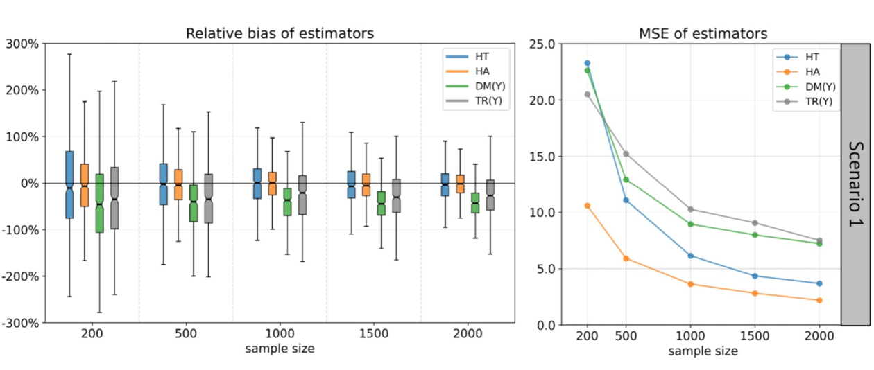
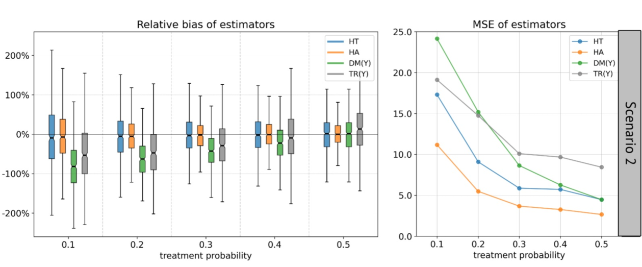
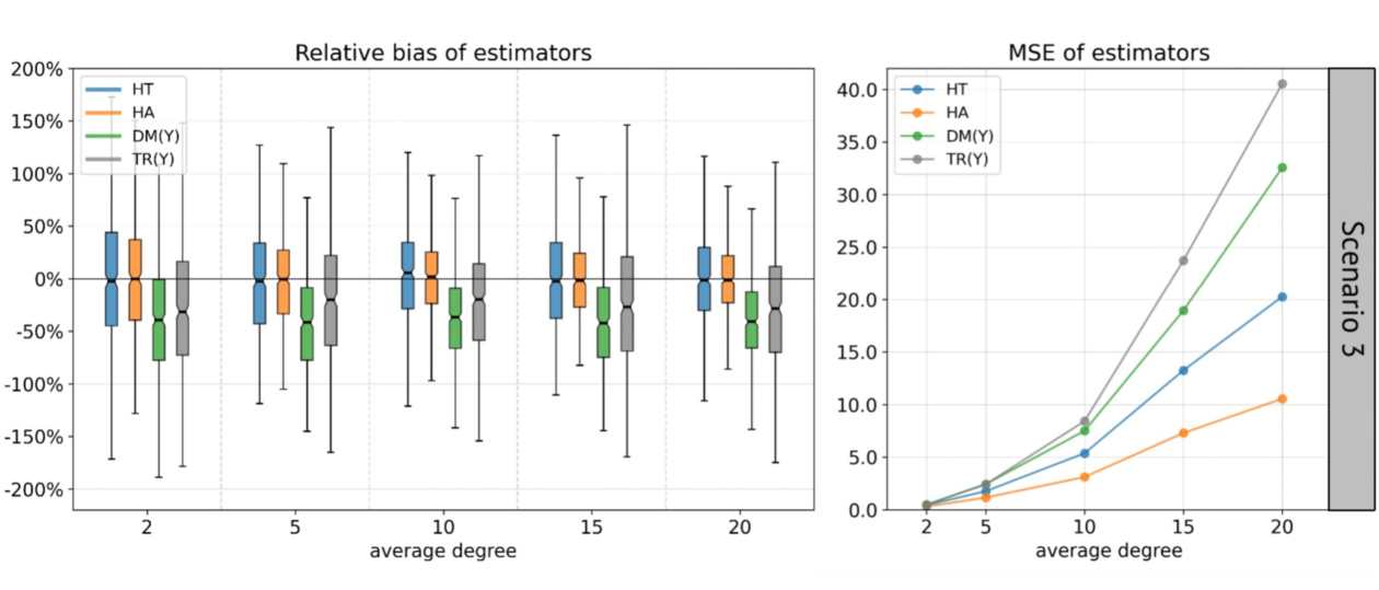
Figure 2: Relative bias and mean squared error of estimators. The legends HT, HA, DM(Y) and TR(Y) correspond to $\hat{\tau}_{\rm HT}$, $\hat{\tau}_{\rm H\acute{A}},\tilde{\tau}(\bm{Y})$ and $\tilde{\tau}_{\rm TR}(\bm{Y})$, respectively.

Figure 3 summarizes the coverage rate of the Wald-type confidence intervals based on different variance estimators $\widehat{V}$, $\widehat{V}(d_{2})$, and $\widehat{V}(\hat{d}_{\infty})$. Under our simulation settings, the 95% confidence intervals based on the variance estimator $\widehat{V}$ could have coverage rates well below the nominal level of $0.95$. The 95% confidence intervals based on $\widehat{V}(d_{2})$ and $\widehat{V}(\hat{d}_{\infty})$ have coverage rates well above the nominal level and sometimes close to 100%, suggesting that these two variance estimators can be overly conservative.

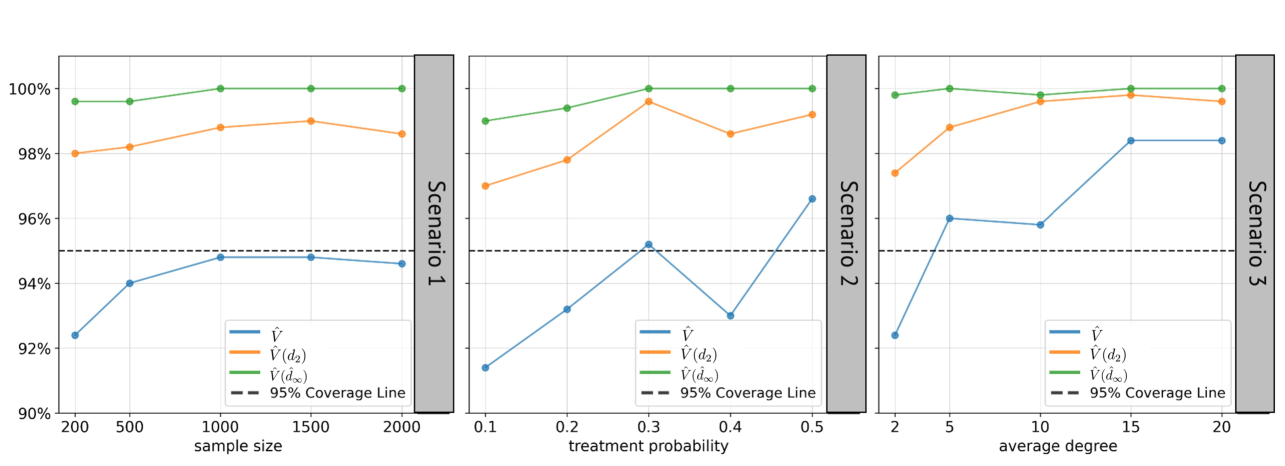
Figure 3: Coverage rate for the 95% confidence intervals based on different variance estimators with varying sample size, degree of network, and treatment probability.

5.2 Performance under different randomization designs

We also compare the proposed estimators under Bernoulli randomization and complete randomization designs. We adopt the Caltech network socfb-Caltech36 from the category of Facebook Networks (Rossi and Ahmed,, 2015), with $n=769$, $d_{2}=43$, and $d_{\infty}=248$. The data-generating process is identical to that in Section 5.1, and we consider treatment probability $p\in\{0.1,0.2,0.3,0.4,0.5\}$. Figure 4 summarises the simulation results. As expected, when the treatment probability $p$ increases, both the relative bias and the mean square errors of estimators $\hat{\tau}_{\rm HT}$ and $\hat{\tau}_{\rm H\acute{A}}$ decrease. Under complete randomization, $\hat{\tau}_{\rm HT}$ and $\hat{\tau}_{\rm H\acute{A}}$ are identical, and all estimators have smaller mean square errors than under the Bernoulli randomization, but the gap becomes smaller as the treatment probability increases. When the sample size $n$ is sufficiently large, which is common in online experiments, the difference between the estimators of the complete randomization and Bernoulli randomization becomes negligible.

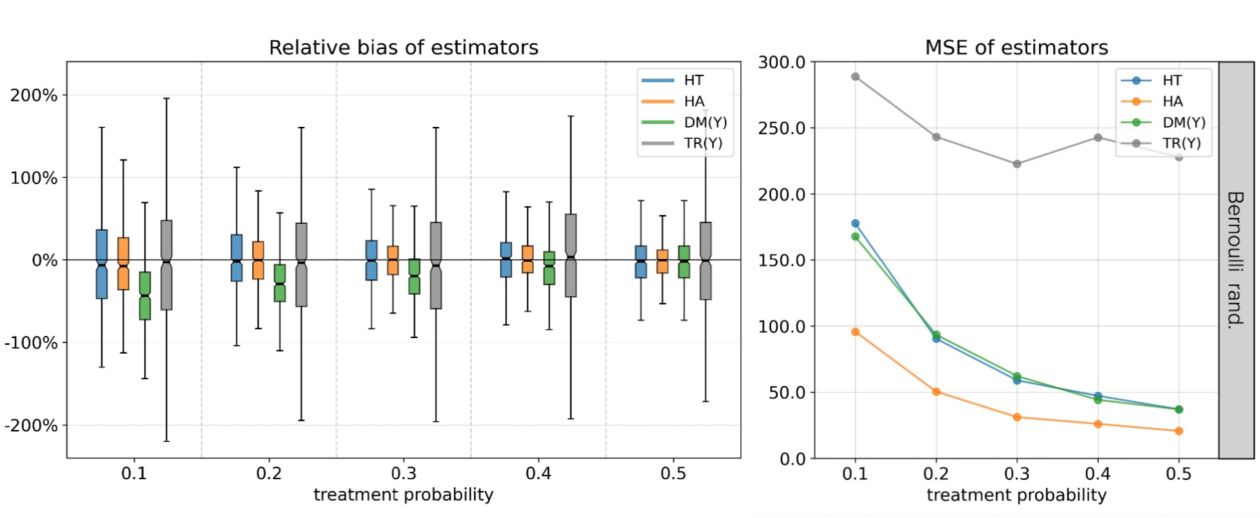
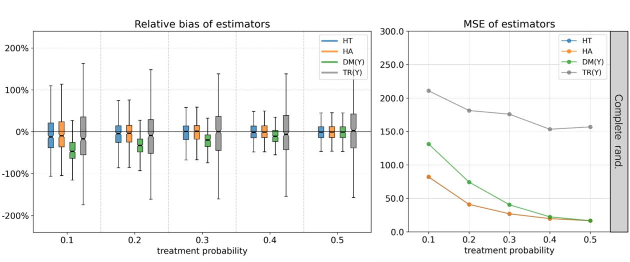
Figure 4: Relative bias and mean squared error of different estimators under Bernoulli and complete randomization.

6 Empirical application

A massive number of A/B tests have been conducted in modern technology companies to evaluate the impact of product updates, such as new user interface designs or recommendation algorithms, on basic functions, user experiences, and other facets of digital platforms. We demonstrate the proposed methods to analyse an A/B test conducted by Weixin Channels, which is a built-in function of Weixin (WeChat in China), enabling all users from Weixin to create and share videos or pictures, and discover content from all users rather than just friends, similar to a news feed. In this A / B test, users in the treatment group (or B) could use an updated version of the recommendation algorithm, aiming to promote the sharing and clicking activity by increasing the ranking of contents liked by both users and their friends, while users in the control group (or A) continued with the previous version. In this experiment, $n=\{4\%$ of all users} are assigned to treatment or control groups by Bernoulli randomization with treatment probability $p_{i}=2/3$. The online experiment lasted for two weeks and elicited over three million interactions among users enrolled in the experiment. Three types of dyadic outcomes $Y_{a,ij}$ for $a=1,2,3$ that measure user interaction activity level and system performance during experimentation periods are of primary interest. The corresponding metrics, defined as $\mathsf{Metric}_{a}=n^{-1}\sum_{i=1}^{n}\sum_{j\in\mathcal{D}_{i}}Y_{a,ij}$ are used to quantify overall user behaviour and system performance. The relative difference of the global average treatment effect is defined as the contrast of metrics in two counterfactual worlds, that is, $\mathsf{RD}_{a}=\sum_{i=1}^{n}\{\sum_{j\in\mathcal{D}_{i}(\bm{1})}Y_{a,ij}(\bm{1})-\sum_{j\in\mathcal{D}_{i}(\bm{0})}Y_{a,ij}(\bm{0})\}/\sum_{i=1}^{n}\sum_{j\in\mathcal{D}_{i}(\bm{0})}Y_{a,ij}(\bm{0})$, which is preferred in A/B tests because it amplifies the effects of small absolute treatment effects into interpretable proportional changes and is also comprehensive for practitioners. The definition of dyadic outcomes and the choice of metrics are closely related to whether the A/B test can detect meaningful differences and support decision-making. For example, if $Y_{a,ij}$ represents the number of messages shared from user $i$ to user $j$, then $\mathsf{Metric}_{a}$ measures the number of messages sent and received per user. However, due to commercial restrictions, we cannot disclose the details of the outcomes and metrics. All data are collected after user approvals and de-identified to protect user privacy. Both A/A tests, where users were randomized into two identical versions of an element, and sample ratio mismatch tests have been performed to check the validity of the treatment allocation and data gathering process.

We are interested in estimating the relative difference of global average treatment effect $\mathsf{RD}_{a}$ and testing the null hypothesis $\mathbb{H}_{0}:\mathsf{RD}_{a}=0$ for $a=1,2,3$. We implement the point estimators $\hat{\tau}_{a,{\rm H\acute{A}}}$ based on dyadic outcomes and $\tilde{\tau}(\bm{Y}_{a})$ based on unit-level outcomes and test the null hypotheses with variance estimators $\widehat{V}_{a},\widehat{V}_{a}(d_{1})$, and $\widehat{V}_{a}(\hat{d}_{\infty})$. The estimator of relative difference $\mathsf{RD}_{a}$ using dyadic outcomes is $\widehat{\mathsf{RD}}_{a,{\rm H\acute{A}}}=(\hat{n}_{0}^{-1}\sum_{i=1}^{n}\sum_{j\neq i}q^{-1}_{ij}\overline{Z}_{ij}Y_{a,ij})^{-1}\hat{\tau}_{a,{\rm H\acute{A}}}$. Similarly, the estimator of $\mathsf{RD}_{a}$ based on unit-level outcomes is $\widetilde{\mathsf{RD}}_{a}=(n^{-1}\sum_{i=1}^{n}q^{-1}_{i}\overline{Z}_{i}Y_{a,i})^{-1}\tilde{\tau}(\bm{Y}_{a})$. The variances of $\widehat{\mathsf{RD}}_{a,{\rm H\acute{A}}},\widetilde{\mathsf{RD}}_{a}$ are estimated using delta method.

Table 1: Relative difference and corresponding p-values of unit-level dyad-level estimators

Quantity	$a=1$		$a=2$		$a=3$
$\widehat{\mathsf{RD}}_{a,{\rm H\acute{A}}}$	1.012%		0.624%		1.124%
p-value $[\widehat{V}_{a}]$	0.193		$0.042$		0.024
p-value [$\widehat{V}_{a}(d_{1})$]	0.230		0.061		0.055
p-value [$\widehat{V}_{a}(\hat{d}_{\infty})$]	0.576		0.383		0.245
$\widetilde{\mathsf{RD}}_{a}$	0.076%		-0.120%		0.285%
p-value	0.821		0.713		0.567

Table 1 reports the relative difference based on unit-level estimator $\tilde{\tau}(\bm{Y}_{a})$ and dyadic estimator $\hat{\tau}_{a,{\rm H\acute{A}}}$, and the corresponding p-values with different variance estimators. The analysis reveals minimal relative difference for $a=1,2$ with relative differences calculated based on $\tilde{\tau}(\bm{Y}_{a})$ statistically indistinguishable from zero, while showing a small positive relative difference ($0.285\%$) for $a=3$. Results based on estimators using dyadic outcomes yield substantially larger relative differences. When using the variance estimator $\widehat{V}_{a}$ for testing the null hypothesis, the test results show that $\mathsf{RD}_{a},a=2,3$ are significantly non-zero at level $\alpha=0.05$; although, using conservative variance estimators $\widehat{V}_{a}(d_{1})$ and $\widehat{V}_{a}(\hat{d}_{\infty})$ leads to less or non-significant results. These analysis results provide empirical evidence in favour of the updated recommendation algorithm, which improves the user experience and ultimately increases user activity. The proposed estimators feature computationally and operationally efficient online implementation using online analytical processing engines such as Spark, and have been seamlessly integrated into the WeChat experimentation platform monitoring for concurrent experiments.

7 Dicussion

Motivated by empirical observations from large-scale online controlled experiments involving message transmission, content dissemination, and VoIP communication systems, this research develops a rigorous methodological framework for analyzing network interference effects at the dyadic level, thereby extending the scope of causal frameworks to account for interdependent outcomes within paired units, particularly in randomized experiments. Our approach addresses the inherent challenges of spillover and mutual influence along dyads, offering novel methodological tools to disentangle interference under dependence structures.

In certain situations, in addition to the dyadic outcomes $Y_{ij}$, some outcomes defined on the users are also of interest at the same time. Building upon the link-sharing scenario in Example 1, we formalize the outcome metrics as follows: let $Y_{ij}$ represent the count of videos shared by user $i$ and viewed by user $j$, while $Y_{ii}$ denotes the number of videos user $i$ watched through external channels (e.g., search engine results). Then we can redefine the upstream aggregated outcomes as $U_{i}=Y_{ii}+\sum_{j\in\mathcal{U}_{i}}Y_{ji}$, and the global average treatment effect are still defined as in (2), representing the total visit views of user $i$. When there is no interference on $Y_{ii}$, i.e., $Y_{ii}(\bm{z})=Y_{ii}(z_{i})$, the Horvitz-Thompson estimator $\hat{\tau}_{\rm HT}$ in (4) can be modified accordingly

$$\hat{\tau}_{\operatorname{Mix-HT}}=\hat{\tau}_{\rm HT}+\frac{1}{n}\sum_{i=1}^{n}\left(\frac{Z_{i}}{p_{i}}-\frac{1-Z_{i}}{q_{i}}\right)Y_{ii}.$$

The theoretical properties can be analogously established for the estimator $\hat{\tau}_{\operatorname{Mix-HT}}$.

Pre-experiment covariates may be involved in the experimental design stage. For example, the treatment assignment probability is determined according to certain covariates, such as stratified randomization and matched-pairs designs. Beyond that, in observational studies, the treatment assignment probability is not available and has to be estimated. It is of interest to extend the proposed framework to such situations to incorporate observed covariates and develop efficient estimation methods. The proposed methods rely on the dyadic interference assumption. However, this assumption may not hold or its validity is diminished in situations where domain knowledge on the interference mechanism is absent. To address this issue, sensitivity analysis is a promising approach, and we briefly illustrate the idea. Suppose $Y_{ij}$ is influenced not only by the treatments applied to units $(i,j)$, but also by the treatments of surrounded upstream neighbors$,i.e.,Y_{ij}(\bm{z})=\alpha_{ij}+\beta_{ij}z_{i}+\gamma_{ij}z_{j}+\lambda_{ij}z_{ij}+\zeta_{ij}\sum_{j\in\mathcal{U}_{i}(\bm{z})}z_{j}.$ This adds an additional layer of complexity to statistical analysis and may introduce bias to the proposed estimators. Suppose there exists some constant $\zeta$ such that the heterogeneous neighbourhood effects can be bounded by a sensitivity parameter $\zeta$, e.g., $\zeta\geq\max_{1\leq i,j\leq n}|\zeta_{ij}|$. In this vein, it is possible to develop a sensitivity analysis approach to assess the robustness of estimators against the violation of dyadic interference within the range of $\zeta$. We plan to pursue such extensions in future work.

Supplementary material

Supplementary Material online includes a detailed analysis of the estimator’s properties under cluster randomization, useful lemmas and detailed proof of the theorems, and additional simulation results under various settings.

Supplementary material for causal inference with dyadic data in randomized experiments 

Yilin Li, Lu Deng, Yong Wang, and Wang Miao

Section A analyzes estimator properties under cluster randomization. Section B contains supporting lemmas and theorem proofs. Additional simulations demonstrating estimator performance are presented in Section C.

Appendix A Estimator under cluster randomization design

A.1 Setting and theoretical discoveries

In the main text, we primarily focused on unit-level randomization designs. However, many other randomization designs also account for network interference. A widely used approach is cluster randomization: suppose $n$ units are partitioned into $L$ disjoint clusters $\{\mathcal{C}_{\ell}\}_{\ell=1}^{L}$ with $\mathcal{C}_{k}\cap\mathcal{C}_{\ell}=\emptyset$ for $1\leq k\neq\ell\leq L$, where the partitioning is derived from the structure of the network structure induced by dyadic outcomes. Under this design, treatment is assigned at the cluster level, with all units within a cluster receiving the same intervention. Formally, for each unit $i\in\mathcal{C}_{\ell}$, the treatment indicator $Z_{i}\sim{\rm Bernoulli}(p_{\ell})$, and $Z_{i}=Z_{j}$ when $i,j\in\mathcal{C}_{\ell}$. For the existence of clusters with any given network sequence, we refer to Leung, (2023).

We define some standard quantities that measure any cluster $\mathcal{C}$ from spectral graph theory (Chung,, 1997). For $\mathsf{z}\in\{0,1\}$ and $\bm{\mathsf{z}}=(\mathsf{z},\ldots,\mathsf{z})$ of length $n$,

Definition S.1 (Number of boundary dyads of cluster).

$\partial_{\mathcal{C}}(\mathsf{z})=\sum_{i\in\mathcal{C}}|\mathcal{N}_{i}(\bm{\mathsf{z}})\setminus\mathcal{C}|$.

Definition S.2 (Number of neighbors within a cluster).

$I_{\mathcal{C}}(\mathsf{z})=\sum_{i\in\mathcal{C}}|\mathcal{N}_{i}(\bm{\mathsf{z}})\cap\mathcal{C}|$.

Definition S.3 (Squared number of neighbors within a cluster).

$S_{\mathcal{C}}(\mathsf{z})=\sum_{i\in\mathcal{C}}|\mathcal{N}_{i}(\bm{\mathsf{z}})\cap\mathcal{C}|^{2}$.

These quantities are defined with respect to a cluster $\mathcal{C}$ and potential neighbors $\mathcal{N}_{i}(\bm{\mathsf{z}})$ under the fully treated ($\bm{\mathsf{z}}=\bm{1}$) or fully control ($\bm{\mathsf{z}}=\bm{0}$) cases. Number of boundary dyads $\partial_{\mathcal{C}}(\mathsf{z})$ counts potential dyadic outcomes where one unit belongs to $\mathcal{C}$ and the other does not. This metric quantifies inter-cluster connectivity. It characterises the degree of separation between clusters, e.g., $\partial_{\mathcal{C}_{\ell}}(\mathsf{z})=0$ implies perfect cluster separation (no edges cross cluster boundaries). The number of internal neighbours $I_{\mathcal{C}}(\mathsf{z})$ is equivalent to twice the number of non-zero dyadic outcomes within $\mathcal{C}$. $S_{\mathcal{C}}(\mathsf{z})$ is defined as the number of squared neighbours, which is also equivalent to the count of 2-hop neighbours within $\mathcal{C}$, reflecting higher-order connectivity. When scaled by cluster size $|\mathcal{C}|$, $|\mathcal{C}|^{-1}I_{\mathcal{C}}(\mathsf{z})$ and $|\mathcal{C}|^{-1}S_{\mathcal{C}}(\mathsf{z})$ mirror the network statistics $d_{1}(\mathsf{z})$ and $d_{2}(\mathsf{z})$ respectively, for the subnetwork induced by $\mathcal{C}$.

Parallel to Theorem 2, we provide the convergence rate of estimators under cluster randomization designs.

Theorem S.1.

Under Assumptions 1 and 2, with cluster randomization design,

$$\hat{\tau}_{\rm HT}-\tau=O_{p}\bigg{(}\max_{\mathsf{z}\in\{0,1\}}\bigg{\{}P_{\mathsf{z}}^{-1}\bigg{(}\sum_{\ell=1}^{L}\{I_{\mathcal{C}_{\ell}}(\mathsf{z})+\partial_{\mathcal{C}_{\ell}}(\mathsf{z})\}\partial_{\mathcal{C}_{\ell}}(\mathsf{z})\bigg{)}^{1/2},P_{\mathsf{z}}^{-1/2}\bigg{(}\sum_{\ell=1}^{L}I^{2}_{\mathcal{C}_{\ell}}(\mathsf{z})\bigg{)}^{1/2}\bigg{\}}n^{-1}\bigg{)},$$

$$\hat{\tau}_{\rm H\acute{A}}-\tau=O_{p}\bigg{(}\max_{\mathsf{z}\in\{0,1\}}\bigg{\{}P_{\mathsf{z}}^{-1}\bigg{(}\sum_{\ell=1}^{L}\{I_{\mathcal{C}_{\ell}}(\mathsf{z})+\partial_{\mathcal{C}_{\ell}}(\mathsf{z})\}\partial_{\mathcal{C}_{\ell}}(\mathsf{z})\bigg{)}^{1/2},P_{\mathsf{z}}^{-1/2}\bigg{(}\sum_{\ell=1}^{L}I^{2}_{\mathcal{C}_{\ell}}(\mathsf{z})\bigg{)}^{1/2}\bigg{\}}n^{-1}\bigg{)}.$$

The convergence rate of the estimator depends on three key factors: $L$, $\partial_{\mathcal{C}_{l}}(\mathsf{z})$ and $I_{\mathcal{C}_{l}}(\mathsf{z})$ for $1\leq l\leq L$. For fixed $L$, the estimator fails to converge, as asymptotic consistency requires $L\rightarrow\infty$. While cluster randomization typically does not achieve faster convergence than unit-level randomization, it can match their rates when the dyadic network satisfies specific structural conditions, e.g., weak inter-cluster dependence or bounded edge boundaries.

Assumption S.1 (Negligible maximum conductance).

$\max_{\mathsf{z}\in\{0,1\}}\max_{1\leq\ell\leq L}\partial_{\mathcal{C}_{\ell}}(\mathsf{z})I^{-1}_{\mathcal{C}_{\ell}}(\mathsf{z})=o(P_{1}P_{0})$.

Conductance $\partial_{\mathcal{C}_{\ell}}(\mathsf{z})I^{-1}_{\mathcal{C}_{\ell}}(\mathsf{z})$ quantifies inter-cluster connectivity relative to intra-cluster density. The requirement $o(P_{1}P_{0})$ ensures that inter-cluster interference becomes asymptotically negligible compared to treatment/control contrasts. Unlike strong assumptions of perfect clustering, this allows sparse cross-cluster interactions, provided they diminish sufficiently fast.

Assumption S.2.

$\max_{\mathsf{z}\in\{0,1\}}\max_{1\leq\ell\leq L}I^{2}_{\mathcal{C}_{\ell}}(\mathsf{z})S^{-1}_{\mathcal{C}_{\ell}}(\mathsf{z})=O(1)$.

(a) Fully-connected clusters

(b) Star-shaped clusters

Figure S.5: Comparison of cluster randomization with different types of clusters.

Recall Definitions S.2 and S.3. $\binom{I_{\mathcal{C}_{\ell}}(\mathsf{z})}{2}$ enumerates all possible pairs of potential dyadic outcomes, while $S_{\mathcal{C}_{\ell}}$ counts the number of 2-hop neighbors in cluster $\mathcal{C}_{\ell}$. Therefore, Assumption S.2 requires that for any two randomly selected dyadic outcomes in a cluster, the probability they share at least one common unit is bounded below. This implies network cohesion where clusters exhibit non-vanishing connectivity. For example, in Figure S.5, the units within each cluster are fully connected on the left, while the clusters are star-shaped on the right. For the fully-connected clusters, if all units has degree $d$ and perferectly clustered, then $I^{2}_{\mathcal{C}_{\ell}}(\mathsf{z})S^{-1}_{\mathcal{C}_{\ell}}(\mathsf{z})=|\mathcal{C}_{\ell}|$. In this case, Assumption S.2 implies bounded cluster size and yields $\hat{\tau}_{\rm HT}$ convergence at $O_{p}(dn^{-1/2})$. For the star-shaped clusters, $I^{2}_{\mathcal{C}_{\ell}}(\mathsf{z})S^{-1}_{\mathcal{C}_{\ell}}(\mathsf{z})\leq 4$ holds naturally due to centralized connectivity. The assumption holds for clusters centralised around focal units, e.g., influencer-centric communities. While cluster randomization typically slows convergence, we identify that under certain network structures, $\hat{\tau}_{\rm HT}$ and $\hat{\tau}_{\rm H\acute{A}}$ match the rate $r_{n}$ under unit-level randomization.

Theorem S.2.

For cluster randomization, under Assumptions 1-2 and S.1-S.2, we have $\hat{\tau}_{\rm HT}-\tau=O_{p}(r_{n})$ and $\hat{\tau}_{\rm H\acute{A}}-\tau=O_{p}(r_{n})$ with $r_{n}$ defined in Theorem 2.

A.2 Numerical demonstration of cluster randomization

We construct synthetic networks $\mathcal{G}$ with $L\in\{100,200,\dots,500\}$ clusters, where each cluster comprises 5 fully connected nodes. A global hub connects to one randomly selected node from every cluster (Figure S.6). This hybrid structure (dense clusters plus star topology) inherently satisfies Assumption S.2 as $L\to\infty$, since intra-cluster cohesion dominates inter-cluster edges through the hub, and the hub ensures $I_{\mathcal{C}_{\ell}}^{2}(\mathsf{z})S^{-1}_{\mathcal{C}_{\ell}}(\mathsf{z})$ remains bounded.

For each edge $(i,j)$ from $\mathcal{G}$, we generate

$$Y_{ij}(z_{i},z_{j})=\underbrace{Y_{ij}(0,0)}_{\text{Baseline}}+\underbrace{\beta_{ij}z_{i}}_{\text{Direct effect of }i}+\underbrace{\gamma_{ij}z_{j}}_{\text{Direct effect of }j}+\underbrace{\lambda_{ij}z_{i}z_{j}}_{\text{Interaction}},$$

with parameters drawn independently as:

$$Y_{ij}(0,0)\sim U(0,1),\quad\beta_{ij}\sim U(0,1),\quad\gamma_{ij}\sim U(-0.5,0),\quad\lambda_{ij}\sim U(0,0.5).$$

The model features heterogeneous effects with varied direct ($\beta_{ij},\gamma_{ij}$) and interaction ($\lambda_{ij}$) terms, where $\gamma_{ij}\leq 0$ captures dampening effects from treated neighbors. The data is fixed once generated. For complete randomization, we assign $n_{1}=\lfloor 5L/3\rfloor$ units to treatment. For cluster randomization, we first apply the Leiden algorithm (Traag et al.,, 2019) with resolution parameter $50$ to partition the network, then randomly assign each cluster to treatment with probability $1/3$. Each randomization design is replicated 500 times with fixed potential outcomes. The design ensures network sparsity through the hub-and-spoke structure, and negative spillover effects via $\gamma_{ij}\in(-0.5,0)$, and (3) bounded cluster influence through the Leiden algorithm’s high-resolution partitioning. The fixed potential outcomes enable direct comparison between randomization schemes.

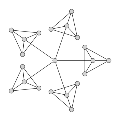
Figure S.6: Visualisation of network with one central unit and five clusters.

As the main text, we evaluate the proposed estimators against two baseline approaches: unit-level weighted estimator $\tilde{\tau}(\bm{Y})$ and exposure threshold estimator $\tilde{\tau}_{\rm TR}(\bm{Y})$. Figure S.7 summarises the simulation results, revealing three key findings. First, the proposed estimator $\hat{\tau}_{\rm H\acute{A}}$ maintains the same MSE magnitudes across different randomization designs. Second, $\hat{\tau}_{\rm HT}$ achieves comparable convergence rates under both complete and cluster randomization schemes for the given network structure. Third, unit-level outcome estimators demonstrate significantly degraded performance when applied to cluster-randomized designs. The robustness of $\hat{\tau}_{\rm H\acute{A}}$ across designs suggests its advantage in handling interference, while the strong performance of $\hat{\tau}_{\rm HT}$ confirms the theoretical rate derived in Theorem S.2.

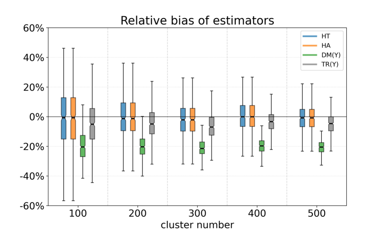
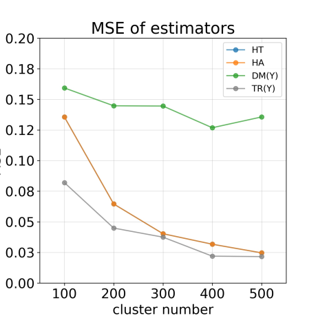
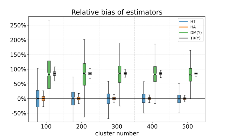
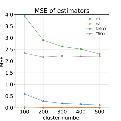
Figure S.7: Relative bias and MSE of different estimators with varying number of clusters $L$ under complete randomization (first row) and cluster randomization (second row).

Appendix B Proof of lemmas and theorems

B.1 Proof of Theorem 1

Proof. Consider the unit-level aggregated outcome variables, namely, the upstream aggregated outcome $U_{i}=\sum_{j\neq i}Y_{ji}$, the downstream aggregated outcome $D_{i}=\sum_{j\neq i}Y_{ij}$, and the sum of these two outcomes $Y_{i}=\sum_{j\neq i}(Y_{ij}+Y_{ji})$. For the unit-level outcome linear weighted estimator in (3), we show that it is biased and inconsistent for the global average treatment effect $\tau$ in general. Recall that we define the following quantities in Section 2,

$$\alpha_{i}=\sum_{j\neq i}\{Y_{ji}(0,1)-Y_{ji}(0,0)\}, \eta_{ji}=Y_{ji}(1,0)-Y_{ji}(0,0),$$

$$\beta_{i}=\sum_{j\neq i}\{Y_{ij}(1,0)-Y_{ij}(0,0)\}, \gamma_{ij}=Y_{ij}(0,1)-Y_{ij}(0,0),$$

$$\lambda_{ij}=Y_{ij}(1,1)-Y_{ij}(1,0)-Y_{ij}(0,1)+Y_{ij}(0,0), \tau_{ij}=Y_{ij}(1,1)-Y_{ij}(0,0).$$

1. For the upstream aggregated potential outcome $U_{i}(\bm{z})$, it can be rewritten as

$$U_{i}(\bm{z})=\sum_{j\neq i}Y_{ji}(z_{j},z_{i})=U_{i}(\bm{0})+\alpha_{i}z_{i}+\sum_{j\neq i}(\eta_{ji}z_{j}+\lambda_{ji}z_{i}z_{j}).$$

The expectation of the estimator $\tilde{\tau}(\bm{U})$ in (3) is

$$E\{\tilde{\tau}(\bm{U})\}= \frac{1}{n}\sum_{i=1}^{n}E\left(\frac{Z_{i}U_{i}}{a_{i}}-\frac{(1-Z_{i})U_{i}}{b_{i}}\right)$$

$$= \frac{1}{n}\sum_{i=1}^{n}E\left\{\left(\frac{Z_{i}}{a_{i}}-\frac{1-Z_{i}}{b_{i}}\right)U_{i}(\bm{Z})\right\}$$

$$= \frac{1}{n}\sum_{i=1}^{n}E\bigg{\{}\left(\frac{Z_{i}}{a_{i}}-\frac{1-Z_{i}}{b_{i}}\right)\bigg{(}U_{i}(\bm{0})+\alpha_{i}Z_{i}+\sum_{j\neq i}(\eta_{ji}Z_{j}+\lambda_{ji}Z_{ji})\bigg{)}\bigg{\}}$$

$$= \frac{1}{n}\sum_{i=1}^{n}\bigg{\{}\bigg{(}\frac{(a_{i}+b_{i})p_{i}-a_{i}}{a_{i}b_{i}}\bigg{)}U_{i}(\bm{0})+\frac{p_{i}}{a_{i}}\alpha_{i}+\sum_{j\neq i}\bigg{(}\frac{(a_{i}+b_{i})p_{ij}-a_{i}p_{j}}{a_{i}b_{i}}\bigg{)}\eta_{ji}+\sum_{j\neq i}\frac{p_{ij}}{a_{i}}\lambda_{ji}\bigg{\}}.$$

Next, we compare each term from the above expectation with the global average treatment effect $\tau$. By definition,

$$\tau=\frac{1}{n}\sum_{i=1}^{n}\bigg{\{}\alpha_{i}+\sum_{j\neq i}(\eta_{ji}+\lambda_{ji})\bigg{\}}.$$

If $E\{\tilde{\tau}(\bm{U})\}=\tau$ for arbitrary choices of parameters, then the following equations must hold

$$(a_{i}+b_{i})p_{i}-a_{i} =0\quad \text{ if }U_{i}(\bm{0})\neq 0,$$ (S.1)

$$p_{i} =a_{i}\quad \text{ if }\alpha_{i}\neq 0,$$

$$p_{ij} =a_{i}\quad \text{ if }\eta_{ji}\neq 0,$$

$$(a_{i}+b_{i})p_{ij}-a_{i}p_{j} =a_{i}b_{i}\quad \text{ if }\lambda_{ji}\neq 0,$$

for all $(i,j)$ pairs.
(A). When the upstream indirect effect or the interactive effect exists ($\eta_{ji}\neq 0$ or $\lambda_{ji}\neq 0$), the possible solutions to the equations are
(a). $\operatorname{pr}(Z_{j}=1\mid Z_{i}=1)=1$ for $(i,j)\in\{(i,j):\eta_{ji}\neq 0\}\cup\{(i,j):\lambda_{ji}\neq 0\}$, and $a_{i}=1$;
(b). $\operatorname{pr}(Z_{j}=0\mid Z_{i}=0)=1$ for $(i,j)\in\{(i,j):\eta_{ji}\neq 0\}\cup\{(i,j):\lambda_{ji}\neq 0\}$.
This is equivalent to always assigning the units with non-zero upstream interference effects to the same group.
(B). When both upstream indirect effect and interactive effect do not exist ($\eta_{ji}=0,\lambda_{ji}=0$), the possible solution to the equations is $a_{i}=p_{i}$ and $b_{i}=1-p_{i}$.

Since the estimator should be unbiased under different choices of parameters, there does not exist a treatment vector $\bm{Z}$ and $a_{i},b_{i}\in(0,1)$ for $1\leq i\leq n$ such that $E\{\tilde{\tau}(\bm{U})\}=\tau$.

2. Similarly, for the downstream aggregated potential outcome $D_{i}(\bm{z})$, we have

$$D_{i}(\bm{z})=\sum_{j\neq i}Y_{ij}(z_{i},z_{j})=D_{i}(\bm{0})+\beta_{i}z_{i}+\sum_{j\neq i}(\gamma_{ij}z_{j}+\lambda_{ij}z_{i}z_{j}),$$

and the expectation of $\tilde{\tau}(\bm{D})$ is

$$E\{\tilde{\tau}(\bm{D})\}=\frac{1}{n}\sum_{i=1}^{n}\bigg{\{}\bigg{(}\frac{(a_{i}+b_{i})p_{i}}{a_{i}b_{i}}-\frac{1}{b_{i}}\bigg{)}D_{i}(\bm{0})+\frac{p_{i}}{a_{i}}\beta_{i}+\sum_{j\neq i}\bigg{(}\frac{(a_{i}+b_{i})p_{ij}}{a_{i}b_{i}}-\frac{p_{j}}{b_{i}}\bigg{)}\gamma_{ij}+\sum_{j\neq i}\frac{p_{ij}}{a_{i}}\lambda_{ij}\bigg{\}}.$$

We also match each coefficient from the above expectation with $\tau$

$$\tau=\frac{1}{n}\sum_{i=1}^{n}\bigg{\{}\beta_{i}+\sum_{j\neq i}(\gamma_{ij}+\lambda_{ij})\bigg{\}}.$$

Therefore, we have the following cases:
(A). When the downstream indirect effect or the interactive effect exists ($\gamma_{ij}\neq 0$ or $\lambda_{ij}\neq 0$), the possible solutions to the equations are
(a). $\operatorname{pr}(Z_{j}=1\mid Z_{i}=1)=1$ for $(i,j)\in\{(i,j):\gamma_{ij}\neq 0\}\cup\{(i,j):\lambda_{ij}\neq 0\}$, and $a_{i}=1$;
(b). $\operatorname{pr}(Z_{j}=0\mid Z_{i}=0)=1$ for $(i,j)\in\{(i,j):\gamma_{ij}\neq 0\}\cup\{(i,j):\lambda_{ij}\neq 0\}$.
(B). When both downstream indirect effect and interactive effect do not exist ($\gamma_{ij}=0,\lambda_{ij}=0$), the possible solution to the equations is $a_{i}=p_{i}$ and $b_{i}=1-p_{i}$.

Hence, there does not exist treatment vector $\bm{Z}$ and $a_{i},b_{i}$ for $1\leq i\leq n$ such that $E\{\tilde{\tau}(\bm{D})\}=\tau$.

3. For the unit-level aggregated potential outcomes $Y_{i}(\bm{z})$,

$$Y_{i}(\bm{z})=Y_{i}(\bm{0})+(\alpha_{i}+\beta_{i})z_{i}+\sum_{j\neq i}\left(\eta_{ji}z_{j}+\lambda_{ji}z_{i}z_{j}+\gamma_{ij}z_{j}+\lambda_{ij}z_{i}z_{j}\right).$$

Then the expectation of $\tilde{\tau}(\bm{Y})$ is

$$E\{\tilde{\tau}(\bm{Y})\}=E\{\tilde{\tau}(\bm{D})+\tilde{\tau}(\bm{U})\}= \frac{1}{n}\sum_{i=1}^{n}\bigg{[}\bigg{(}\frac{(a_{i}+b_{i})p_{i}}{a_{i}b_{i}}-\frac{1}{b_{i}}\bigg{)}Y_{i}(\bm{0})+\frac{p_{i}}{a_{i}}(\alpha_{i}+\beta_{i})$$

$$+\sum_{j\neq i}\bigg{(}\frac{(a_{i}+b_{i})p_{ij}}{a_{i}b_{i}}-\frac{p_{j}}{b_{i}}\bigg{)}(\gamma_{ij}+\eta_{ji})+\sum_{j\neq i}\frac{p_{ij}}{a_{i}}(\lambda_{ij}+\lambda_{ji})\bigg{]}.$$

The following equations hold due to the symmetry of the upstream and downstream aggregation

$$\sum_{i=1}^{n}\alpha_{i}=\sum_{i=1}^{n}\sum_{j\neq i}\gamma_{ij},\quad\sum_{i=1}^{n}\beta_{i}=\sum_{i=1}^{n}\sum_{j\neq i}\eta_{ji},\quad\sum_{i=1}^{n}\sum_{j\neq i}\lambda_{ij}=\sum_{i=1}^{n}\sum_{k\neq i}\lambda_{ki}.$$

Therefore, the following restrictions suffice for $E\{\tilde{\tau}(\bm{Y})\}=\tau$

$$(a_{i}+b_{i})p_{i} =a_{i}\quad \text{ if }\alpha_{i}\neq 0\text{ or }\beta_{i}\neq 0$$

$$p_{i} =a_{i}\quad \text{ if }\alpha_{i}+\beta_{i}\neq 0,$$

$$2p_{ij} =a_{i}\quad \text{ if }\gamma_{ij}+\eta_{ji}\neq 0,$$

$$(a_{i}+b_{i})p_{ij} =0\quad \text{ if }\lambda_{ij}+\lambda_{ji}\neq a_{i}p_{j}.$$

The unique solution to the above equations is $a_{i}=b_{i}=p_{i}=1/2$ and $Z_{i}\sim\text{Bernoulli}(1/2)$ independently for $1\leq i\leq n$.

For the inconsistency of the estimators, we adopt a similar argument as Proposition 1 and 2 of Sävje et al., (2021) and claim that the estimators in (3) have either infinite variance or are consistent for the mean $E\{\tilde{\tau}(\bm{Y})\}$, which is unequal to $\tau$ except that $a_{i}=b_{i}=p_{i}=1/2$ and $Z_{i}\sim\text{Bernoulli}(1/2)$ independently for $1\leq i\leq n$ under Assumption 1 and 2.

B.2 Proof of Theorem 2

Proof. For notational simplicity, we let

$${\mu}_{1}=\frac{1}{n}\sum_{i=1}^{n}\sum_{j\neq i}Y_{ij}(1,1), {\mu}_{0}=\frac{1}{n}\sum_{i=1}^{n}\sum_{j\neq i}Y_{ij}(0,0),$$

$$\hat{\mu}_{1}=\frac{1}{n}\sum_{i=1}^{n}\sum_{j\neq i}Z_{ij}Y_{ij}/p_{ij}, \hat{\mu}_{0}=\frac{1}{n}\sum_{i=1}^{n}\sum_{j\neq i}\overline{Z}_{ij}Y_{ij}/q_{ij},$$ (S.2)

$$\hat{\mu}_{1,\operatorname{H\acute{A}}}=\sum_{i=1}^{n}\sum_{j\neq i}\frac{Z_{ij}Y_{ij}}{p_{ij}}\Big{/}\sum_{i=1}^{n}\frac{Z_{i}}{p_{i}}, \hat{\mu}_{0,\operatorname{H\acute{A}}}=\sum_{i=1}^{n}\sum_{j\neq i}\frac{\overline{Z}_{ij}Y_{ij}}{q_{ij}}\Big{/}\sum_{i=1}^{n}\frac{\overline{Z}_{i}}{q_{i}}.$$

For the estimator $\hat{\tau}_{\rm HT}=\hat{\mu}_{1}-\hat{\mu}_{0}$, it is unbiased under Bernoulli randomization, and the variance is

$$\operatorname{var}(\hat{\tau}_{\rm HT})=\operatorname{var}(\hat{\mu}_{1})+\operatorname{var}(\hat{\mu}_{0})-2\operatorname{cov}(\hat{\mu}_{1},\hat{\mu}_{0}).$$

We calculate the above three terms. For the variance of $\hat{\mu}_{1}$, we have

$$\operatorname{var}(\hat{\mu}_{1})=\operatorname{var}\left(\frac{1}{n}\sum_{i=1}^{n}\sum_{j\neq i}\frac{Z_{ij}Y_{ij}}{p_{ij}}\right)=\frac{1}{n^{2}}\sum_{i=1}^{n}\sum_{j\neq i}\sum_{k=1}^{n}\sum_{l\neq k}\operatorname{cov}\left(\frac{Z_{ij}Y_{ij}}{p_{ij}},\frac{Z_{kl}Y_{kl}}{p_{kl}}\right).$$ (S.3)

Next, we analyse the estimator under Bernoulli and complete randomization designs.

1. (Bernoulli randomization) We let $\zeta_{i}=q_{i}/p_{i}$ denote the odds of treated probability of unit $i$ and $\zeta_{ij}=(1-p_{ij})/p_{ij}$ denote the odds of treated probability that unit $(i,j)$ are both treated. The variance decomposition terms in (S.3) can be categorised by subscript overlap patterns:
(A). Both subscripts overlap:
(a). If $i=k$ and $j=l$, we have

$$\operatorname{cov}\left(\frac{Z_{ij}Y_{ij}}{p_{ij}},\frac{Z_{kl}Y_{kl}}{p_{kl}}\right)=p_{ij}^{-2}\operatorname{var}\left(Z_{ij}Y_{ij}\right)=p_{ij}^{-2}Y_{ij}(1,1)^{2}\operatorname{var}\left(Z_{ij}\right)=\zeta_{ij}Y_{ij}(1,1)^{2}.$$

(b). If $i=l$ and $j=k$,

$$\operatorname{cov}\left(\frac{Z_{ij}Y_{ij}}{p_{ij}},\frac{Z_{kl}Y_{kl}}{p_{kl}}\right)=p_{ij}^{-2}\operatorname{cov}\left(Z_{ij}Y_{ij},Z_{ji}Y_{ji}\right)=\zeta_{ij}Y_{ij}(1,1)Y_{ji}(1,1).$$

(B). One entry of the subscripts is identical, while the other one is not:
(a). If $i=k$ and $j\neq l$,

$$\operatorname{cov}\left(\frac{Z_{ij}Y_{ij}}{p_{ij}},\frac{Z_{kl}Y_{kl}}{p_{kl}}\right)=\frac{Y_{ij}(1,1)Y_{il}(1,1)\operatorname{cov}\left(Z_{ij},Z_{il}\right)}{p_{i}^{2}p_{j}p_{l}}=\zeta_{i}Y_{ij}(1,1)Y_{il}(1,1).$$

(b). If $i=l$ and $j\neq k$,

$$\operatorname{cov}\left(\frac{Z_{ij}Y_{ij}}{p_{ij}},\frac{Z_{kl}Y_{kl}}{p_{kl}}\right) = \zeta_{i}Y_{ij}(1,1)Y_{ki}(1,1).$$

(c). If $i\neq k$ and $j=l$,

$$\operatorname{cov}\left(\frac{Z_{ij}Y_{ij}}{p_{ij}},\frac{Z_{kl}Y_{kl}}{p_{kl}}\right) = \zeta_{j}Y_{ij}(1,1)Y_{kj}(1,1).$$

(d). If $i\neq l$ and $j=k$,

$$\operatorname{cov}\left(\frac{Z_{ij}Y_{ij}}{p_{ij}},\frac{Z_{kl}Y_{kl}}{p_{kl}}\right) = \zeta_{j}Y_{ij}(1,1)Y_{jl}(1,1).$$

(C). None of the subscripts is identical, e.g., $i\neq k$ and $j\neq l$. The covariance is

$$\operatorname{cov}\left(\frac{Z_{ij}Y_{ij}}{p_{ij}},\frac{Z_{kl}Y_{kl}}{p_{kl}}\right)=\frac{Y_{ij}(1,1)Y_{kl}(1,1)}{p_{ij}p_{kl}}\operatorname{cov}\left(Z_{ij},Z_{kl}\right)=0,$$ (S.4)

since $Z_{ij}$ and $Z_{kl}$ are independent under Bernoulli randomization.
Combining all above, the variance of $\hat{\mu}_{1}$ is

$$\operatorname{var}(\hat{\mu}_{1})=\frac{1}{n^{2}}\sum_{i=1}^{n}\sum_{j\neq i}\bigg{(} \zeta_{ij}Y_{ij}(1,1)\{Y_{ij}(1,1)+Y_{ji}(1,1)\}$$ (S.5)

$$+\sum_{\begin{subarray}{c}k\neq i\\ k\neq j\end{subarray}}\zeta_{i}\{Y_{ij}(1,1)+Y_{ji}(1,1)\}\left\{Y_{ik}(1,1)+Y_{ki}(1,1)\right\}\bigg{)}.$$

Recall that the sets of upstream, downstream and total neighbors of unit $i$ defined by the potential dyadic outcomes are $\mathcal{D}_{i}(\bm{1})=\{j:Y_{ij}(1,1)\neq 0\},\mathcal{U}_{i}(\bm{1})=\{j:Y_{ji}(1,1)\neq 0\}$ and $\mathcal{N}_{i}(\bm{1})=\mathcal{D}_{i}(\bm{1})\cup\mathcal{U}_{i}(\bm{1})$, respectively. Under Assumption 2, the variance can be upper bounded by

$$\operatorname{var}(\hat{\mu}_{1}) = \frac{1}{n^{2}}\sum_{i=1}^{n}\zeta_{ij}\bigg{(}\sum_{j\in\mathcal{D}_{i}(\bm{1})}Y_{ij}(1,1)^{2}+\sum_{j\in\mathcal{U}_{i}(\bm{1})\cap\mathcal{D}_{i}(\bm{1})}Y_{ji}(1,1)Y_{ij}(1,1)\bigg{)}$$

$$+\frac{1}{n^{2}}\sum_{i=1}^{n}\sum_{j\in\mathcal{D}_{i}(\bm{1})}\zeta_{i}\bigg{(}\sum_{k\in\mathcal{D}_{i}(\bm{1})}Y_{ij}(1,1)Y_{ik}(1,1)+\sum_{k\in\mathcal{U}_{i}(\bm{1})}Y_{ij}(1,1)Y_{ki}(1,1)\bigg{)}$$

$$+\frac{1}{n^{2}}\sum_{i=1}^{n}\sum_{j\in\mathcal{U}_{i}(\bm{1})}\zeta_{i}\bigg{(}\sum_{k\in\mathcal{D}_{i}(\bm{1})}Y_{ji}(1,1)Y_{ik}(1,1)+\sum_{k\in\mathcal{U}_{i}(\bm{1})}Y_{ji}(1,1)Y_{ki}(1,1)\bigg{)}$$

$$\leq \frac{2K^{2}}{n^{2}P_{1}}\bigg{(}\sum_{i=1}^{n}P_{1}^{-1}|\mathcal{N}_{i}(\bm{1})|+\sum_{i=1}^{n}\sum_{j\in\mathcal{N}_{i}(\bm{1})}|\mathcal{N}_{i}(\bm{1})|\bigg{)}$$

$$= \frac{2K^{2}}{n}\left(\frac{d_{1}(1)}{P_{1}^{2}}+\frac{d_{2}(1)}{P_{1}}\right)$$

$$= O\left(\left\{P_{1}^{-2}d_{1}(1)+P_{1}^{-1}d_{2}(1)\right\}n^{-1}\right).$$

The first inequality holds since $\max_{1\leq i\neq j\leq n}\max_{z_{i},z_{j}\in\{0,1\}}|Y_{ij}(z_{i},z_{j})|\leq K$, $\max_{1\leq i\leq n}\zeta_{i}\leq P_{1}^{-1}$ and $\max_{1\leq i,j\leq n}\zeta_{ij}\leq P_{1}^{-2}$. Similarly, one can show that $\operatorname{var}(\hat{\mu}_{0})=O\left(\left\{P_{0}^{-2}d_{1}(0)+P_{0}^{-1}d_{2}(0)\right\}n^{-1}\right).$ It is clear that $E(\hat{\mu}_{\mathsf{z}})=\mu_{\mathsf{z}}$ for $\mathsf{z}\in\{0,1\}$. By applying the Markov’s inequality, for $\epsilon=\{d_{1}(1)^{1/2}P_{1}^{-1}+d_{2}(1)^{1/2}P_{1}^{-1/2}\}Kn^{-1/2}$, we have

$$\operatorname{pr}\left(|\hat{\mu}_{1}-\mu_{1}|>\epsilon\right)\leq\frac{\operatorname{var}\left(\hat{\mu}_{1}\right)}{\epsilon^{2}}=O(1).$$

Therefore,

$$\hat{\mu}_{1}-\mu_{1}=O_{p}\left(\left\{P_{1}^{-1}d_{1}(1)^{1/2}+P_{1}^{-1/2}d_{2}(1)^{1/2}\right\}n^{-1/2}\right).$$

Similarly, we have

$$\hat{\mu}_{0}-\mu_{0}=O_{p}\left(\left\{P_{0}^{-1}d_{1}(0)^{1/2}+P_{0}^{-1/2}d_{2}(0)^{1/2}\right\}n^{-1/2}\right).$$

Hence, the Horvitz-Thompson estimator $\hat{\tau}_{\rm HT}-\tau=\hat{\mu}_{1}+\hat{\mu}_{0}-\mu_{1}-\mu_{0}={O}_{p}\left(r_{n}\right).$

For the Hájek-type estimator, the variances of the denominator $\hat{n}_{1}$ and $\hat{n}_{0}$ are

$$\operatorname{var}\left(\hat{n}_{1}\right) = \operatorname{var}\left(\sum_{i=1}^{n}\frac{Z_{i}}{p_{i}}\right)=\sum_{i=1}^{n}\frac{p_{i}q_{i}}{p_{i}}=\sum_{i=1}^{n}q_{i},$$

$$\operatorname{var}\left(\hat{n}_{0}\right) = \operatorname{var}\left(\sum_{i=1}^{n}\frac{(1-Z_{i})}{E(1-Z_{i})}\right)=\sum_{i=1}^{n}\frac{p_{i}q_{i}}{q_{i}}=\sum_{i=1}^{n}p_{i}.$$

Letting $\bar{p}=n^{-1}\sum_{i=1}^{n}p_{i}$, we see that $\hat{n}_{1}/n-1=O_{p}((1-\bar{p})^{1/2}n^{-1/2})$ and $\hat{n}_{0}/n-1=O_{p}(\bar{p}^{1/2}n^{-1/2})$ by applying the Markov’s inequality. Hence, the first part of Hájek estimator converges as follows

$$\hat{\mu}_{\rm 1,H\acute{A}}-\mu_{1} = \frac{n-\hat{n}_{1}}{\hat{n}_{1}}\hat{\mu}_{\rm 1}+\hat{\mu}_{\rm 1}-\mu_{1}=O_{p}\left(\left\{P_{1}^{-1}d_{1}(1)^{1/2}+P_{1}^{-1/2}d_{2}(1)^{1/2}\right\}n^{-1/2}\right).$$ (S.6)

Similar arguments hold for $\hat{\mu}_{\rm 0,H\acute{A}}$. The Hájek estimator exhibits the same convergence rate, that is,

$$\hat{\tau}_{\rm H\acute{A}}-\tau=\hat{\mu}_{1,\operatorname{H\acute{A}}}-\hat{\mu}_{0,\operatorname{H\acute{A}}}-\mu_{1}+\mu_{0}={O}_{p}\left(r_{n}\right).$$

2. (Complete randomization) It is direct to show that the estimator $\hat{\tau}_{\rm HT}$ is unbiased. Next, we consider each covariance term in (S.3) under complete randomization. Akin to the proof of Bernoulli randomization, there are three categories in terms of subscript overlap:
(A). The subscripts are identical:
(a). If $i=k$ and $j=l$, we have

$$\operatorname{cov}\left(\frac{Z_{ij}Y_{ij}}{p_{ij}},\frac{Z_{kl}Y_{kl}}{p_{kl}}\right)=\frac{\operatorname{var}\left(Z_{ij}Y_{ij}\right)}{p_{ij}^{2}}=\frac{(1-p_{ij})Y_{ij}(1,1)^{2}}{p_{ij}}=\left(\frac{n(n-1)}{n_{1}(n_{1}-1)}-1\right)Y_{ij}(1,1)^{2}.$$

(b). If $i=l$ and $j=k$,

$$\operatorname{cov}\left(\frac{Z_{ij}Y_{ij}}{p_{ij}},\frac{Z_{kl}Y_{kl}}{p_{kl}}\right)=\frac{\operatorname{cov}\left(Z_{ij}Y_{ij},Z_{ji}Y_{ji}\right)}{p_{ij}^{2}}=\left(\frac{n(n-1)}{n_{1}(n_{1}-1)}-1\right)Y_{ij}(1,1)Y_{ji}(1,1).$$

(B). One entry of the subscripts is identical, while the other one is different:
(a). If $i=k$ and $j\neq l$,

$$\operatorname{cov}\left(\frac{Z_{ij}Y_{ij}}{p_{ij}},\frac{Z_{kl}Y_{kl}}{p_{kl}}\right)=\left(\frac{n(n-1)(n_{1}-2)}{n_{1}(n_{1}-1)(n-2)}-1\right)Y_{ij}(1,1)Y_{il}(1,1).$$

(b). If $i=l$ and $j\neq k$,

$$\operatorname{cov}\left(\frac{Z_{ij}Y_{ij}}{p_{ij}},\frac{Z_{kl}Y_{kl}}{p_{kl}}\right)=\left(\frac{n(n-1)(n_{1}-2)}{n_{1}(n_{1}-1)(n-2)}-1\right)Y_{ij}(1,1)Y_{ki}(1,1).$$

(c). If $i\neq k$ and $j=l$,

$$\operatorname{cov}\left(\frac{Z_{ij}Y_{ij}}{p_{ij}},\frac{Z_{kl}Y_{kl}}{p_{kl}}\right)=\left(\frac{n(n-1)(n_{1}-2)}{n_{1}(n_{1}-1)(n-2)}-1\right)Y_{ij}(1,1)Y_{kj}(1,1).$$

(d). If $i\neq l$ and $j=k$,

$$\operatorname{cov}\left(\frac{Z_{ij}Y_{ij}}{p_{ij}},\frac{Z_{kl}Y_{kl}}{p_{kl}}\right)=\left(\frac{n(n-1)(n_{1}-2)}{n_{1}(n_{1}-1)(n-2)}-1\right)Y_{ij}(1,1)Y_{jl}(1,1).$$

(C). None of the subscripts is identical, e.g., $i\neq k$ and $j\neq l$. The covariance is

$$\operatorname{cov}\left(\frac{Z_{ij}Y_{ij}}{p_{ij}},\frac{Z_{kl}Y_{kl}}{p_{kl}}\right)=\frac{Y_{ij}(1,1)Y_{kl}(1,1)\operatorname{cov}\left(Z_{ij},Z_{kl}\right)}{p_{ij}p_{jk}}=\frac{n(n-1)(n_{1}-2)(n_{1}-3)}{n_{1}(n_{1}-1)(n-2)(n-3)}-1.$$

Recalling that under complete randomization, we have $P_{1}=n_{1}/n$ and $P_{0}=n_{0}/n$. Hence,

$$\frac{n(n-1)}{n_{1}(n_{1}-1)} =P_{1}^{-2}\left(1+\frac{P_{0}}{nP_{1}-1}\right)=P_{1}^{-2}+O\left(n^{-1}p^{-3}\right),$$

$$\frac{n(n-1)(n_{1}-2)}{n_{1}(n_{1}-1)(n-2)} =P_{1}^{-2}\left(1+\frac{P_{0}}{nP_{1}-1}\right)\left(P_{1}+\frac{2(P_{1}-1)}{n-2}\right)=P_{1}^{-1}+O\left(n^{-1}P_{1}^{-1}\right),$$

$$\frac{n(n-1)(n_{1}-2)(n_{1}-3)}{n_{1}(n_{1}-1)(n-2)(n-3)} =P_{1}^{-2}\left(1+\frac{P_{0}}{nP_{1}-1}\right)\left(P_{1}+\frac{2(P_{1}-1)}{n-2}\right)\left(P_{1}+\frac{3(P_{1}-1)}{n-3}\right)=1+O\left(n^{-1}P_{1}^{-1}\right).$$

Combining all above, the variance of $\hat{\mu}_{1}$ is

$$\operatorname{var}(\hat{\mu}_{1}) \lesssim \frac{1}{n^{2}}\sum_{i=1}^{n}\left(P_{1}^{-2}-1\right)\bigg{(}\sum_{j\in\mathcal{D}_{i}(\bm{1})}Y_{ij}(1,1)^{2}+\sum_{j\in\mathcal{U}_{i}(\bm{1})\cap\mathcal{D}_{i}(\bm{1})}Y_{ji}(1,1)Y_{ij}(1,1)\bigg{)}$$

$$+\frac{1}{n^{2}}\sum_{i=1}^{n}\sum_{j\in\mathcal{D}_{i}(\bm{1})}\left(P_{1}^{-1}-1\right)\bigg{(}\sum_{k\in\mathcal{D}_{i}(\bm{1})}Y_{ij}(1,1)Y_{ik}(1,1)+\sum_{k\in\mathcal{U}_{i}(\bm{1})}Y_{ij}(1,1)Y_{ki}(1,1)\bigg{)}$$

$$+\frac{1}{n^{2}}\sum_{i=1}^{n}\sum_{j\in\mathcal{U}_{i}(\bm{1})}\left(P_{1}^{-1}-1\right)\bigg{(}\sum_{k\in\mathcal{D}_{i}(\bm{1})}Y_{ji}(1,1)Y_{ik}(1,1)+\sum_{k\in\mathcal{U}_{i}(\bm{1})}Y_{ji}(1,1)Y_{ki}(1,1)\bigg{)}$$

$$+\frac{1}{n^{3}}\sum_{i=1}^{n}\sum_{j\in\mathcal{D}_{i}(\bm{1})}\sum_{k\neq i,k\neq j}\sum_{l\in\mathcal{D}_{k}(\bm{1}),l\neq i,l\neq j}P_{1}^{-1}Y_{ij}(1,1)Y_{kl}(1,1)$$

$$\leq \frac{2K^{2}}{n^{2}P_{1}}\bigg{[}\sum_{i=1}^{n}P_{1}^{-1}|\mathcal{N}_{i}(\bm{1})|+\sum_{i=1}^{n}|\mathcal{N}_{i}(\bm{1})|^{2}+\sum_{i=1}^{n}\sum_{j\in\mathcal{N}_{i}(\bm{1})}|\mathcal{N}_{j}(\bm{1})|+\left\{\binom{nd_{1}(1)}{2}-nd_{2}(1)\right\}n^{-1}\bigg{]}$$

$$= \frac{2K^{2}}{n}\left(\frac{d_{1}(1)}{P_{1}^{2}}+\frac{2d_{2}(1)}{P_{1}}+\frac{d_{1}(1)^{2}}{2P_{1}}-\frac{d_{1}(1)^{2}}{2nP_{1}}-\frac{d_{2}(1)}{n^{2}P_{1}}\right)$$

$$= O\left(\left\{P_{1}^{-2}d_{1}(1)+P_{1}^{-1}d_{2}(1)\right\}n^{-1}\right).$$

The last equation holds since $d_{2}(\mathsf{z})\geq d_{1}(\mathsf{z})^{2}$. Similarly, one can show that under complete randomization $\operatorname{var}(\hat{\mu}_{0})=O\left(\left\{P_{0}^{-2}d_{1}(0)+P_{0}^{-1}d_{2}(0)\right\}n^{-1}\right).$ Therefore, we have $E(\hat{\tau}_{\rm HT}-\tau)^{2}=O(r_{n}^{2})$. Similar as Bernoulli randomization, we claim that the Horvitz-Thompson estimator converges by $\hat{\tau}_{\rm HT}-\tau={O}_{p}\left(r_{n}\right).$ For the Hájek estimator, notice that $\hat{n}_{1}=\sum_{i=1}^{n}Z_{i}/p_{i}=n_{1}/(n_{1}/n)=n$ and $\hat{n}_{0}=n$, so the $\hat{\tau}_{\operatorname{H\acute{A}}}$ and $\hat{\tau}_{\rm HT}$ are identical, which directly implies $\hat{\tau}_{\operatorname{H\acute{A}}}-\tau={O}_{p}\left(r_{n}\right).$

B.3 Proof of Theorem 3

Proof. By Assumption 2, the treated probabilities lie within $[P_{1},1-P_{0}]$. If $P_{1},P_{0}$ are fixed, then

$$\hat{\tau}_{\rm HT}-\tau=O_{p}\left(\max_{\mathsf{z}\in\{0,1\}}\{d_{1}(\mathsf{z}),d_{2}(\mathsf{z})^{1/2}\}n^{-1/2}\right).$$

For $\mathsf{z}\in\{0,1\}$, $d_{1}(\mathsf{z})=n^{-1}\sum_{i=1}^{n}|\mathcal{N}_{i}(\bm{\mathsf{z}})|\leq n^{-1}\sum_{i=1}^{n}|\mathcal{N}_{i}(\bm{\mathsf{z}})|^{2}=d_{2}(\mathsf{z})$ by the fact that $|\mathcal{N}_{i}(\bm{\mathsf{z}})|$ is non-negative integers for $1\leq i\leq n$. Hence, we have

$$\hat{\tau}_{\rm HT}-\tau=O_{p}\left(\max_{\mathsf{z}\in\{0,1\}}d_{2}(\mathsf{z})^{1/2}n^{-1/2}\right)\quad\text{and }\quad\hat{\tau}_{\operatorname{H\acute{A}}}-\tau=O_{p}\left(\max_{\mathsf{z}\in\{0,1\}}d_{2}(\mathsf{z})^{1/2}n^{-1/2}\right).$$

To show the asymptotic normality of $\hat{\tau}_{\rm HT}$ and $\hat{\tau}_{\rm H\acute{A}}$ under Bernoulli randomization, we apply Stein’s method with dependency neighbours. The results collected from Theorem 3.6 of Ross, (2011) are summarised here.

Lemma S.1.

Let $X_{1},\dots,X_{n}$ be random variables with $E(X_{i})=0,\sigma_{n}^{2}={\rm var}(\sum_{i=1}^{n}X_{i})>0$, and $E(X_{i}^{4})<\infty$. The dependency neighbors of $X_{i}$ is $\mathcal{O}_{i}$ for $1\leq i\leq n$. Then,

$$d\big{(}\sigma_{n}^{-1}\sum_{i=1}^{n}X_{i},Z\big{)}\leq\sigma_{n}^{-3/2}\sum_{i=1}^{n}\sum_{j,k\in\mathcal{O}_{i}}E\left|X_{i}X_{j}X_{k}\right|+3\sigma_{n}^{-2}\max_{1\leq i\leq n}|\mathcal{O}_{i}|^{3/2}\bigg{(}\sum_{i=1}^{n}E(X_{i}^{4})\bigg{)}^{1/2}.$$ (S.7)

where $Z$ is a standard normal random variable and

$$d(X,Y)=\sup_{h:|h(x)-h(y)|\leq|x-y|}\left|\int h(x)dF_{X}(x)-\int h(x)dF_{Y}(x)\right|,$$

denotes the Wasserstein metric of two random variables $X,Y$.

Lemma S.2.

With Bernoulli randomization design under Assumptions 1-2, the Wasserstein metric of estimator $\hat{\tau}_{\rm HT}$ and a standard normal random variable $Z$ is bounded by

$$d(\hat{\tau}_{\rm HT},Z) \lesssim {\rm var}(\hat{\tau}_{\rm HT})^{-3/2}n^{-2}\max_{\mathsf{z}\in\{0,1\}}\{d_{1}(\mathsf{z})d_{\infty}(\mathsf{z})^{2}\}\max_{\mathsf{z}\in\{0,1\}}P_{\mathsf{z}}^{-2}$$ (S.8)

$$+ {\rm var}(\hat{\tau}_{\rm HT})^{-1}n^{-3/2}\max_{\mathsf{z}\in\{0,1\}}\{d_{1}(\mathsf{z})^{1/2}d_{\infty}(\mathsf{z})^{3/2}\}\max_{\mathsf{z}\in\{0,1\}}P_{\mathsf{z}}^{-3}.$$

Proof. We apply Lemma S.1 to estimator $\hat{\tau}_{\rm HT}$ in the following. We let $W_{ij}=p_{ij}^{-1}Z_{ij}-1$ and $\overline{W}_{ij}=q_{ij}^{-1}\overline{Z}_{ij}-1$, and define $R_{ij}=W_{ij}Y_{ij}(1,1)-\overline{W}_{ij}Y_{ij}(0,0).$ Hence, $\hat{\tau}_{\rm HT}-\tau=n^{-1}\sum_{i=1}^{n}\sum_{j\neq i}R_{ij}$. We replace the random variables $X_{i}$ in Lemma S.1 with $R_{ij}$. For each dyad $(i,j)$, the corresponding dependency neighbors $\mathcal{O}_{ij}$ of $(i,j)$ belongs to one of the four sets,

$$\mathcal{O}_{ij}\subseteq \left\{(k,i):k\in\mathcal{U}_{i}(\bm{0})\cup\mathcal{U}_{i}(\bm{1})\right\}\cup\left\{(i,k):k\in\mathcal{D}_{i}(\bm{0})\cup\mathcal{D}_{i}(\bm{1})\right\}$$

$$\cup \left\{(k,j):k\in\mathcal{U}_{j}(\bm{0})\cup\mathcal{U}_{j}(\bm{1})\right\}\cup\left\{(j,k):k\in\mathcal{D}_{j}(\bm{0})\cup\mathcal{D}_{j}(\bm{1})\right\}.$$

Therefore, the number of dependency neighborhood $\mathcal{O}_{ij}$ is upper bounded by

$$|\mathcal{O}_{ij}|\leq|\mathcal{N}_{i}(\bm{0})|+|\mathcal{N}_{i}(\bm{1})|+|\mathcal{N}_{j}(\bm{0})|+|\mathcal{N}_{j}(\bm{1})|\leq 4\max_{\mathsf{z}\in\{0,1\}}d_{\infty}(\mathsf{z}).$$

We restate the results in Lemma S.1 with our notations,

$$d(\hat{\tau}_{\rm HT},Z)\leq {\rm var}(\hat{\tau}_{\rm HT})^{-3/2}\sum_{i=1}^{n}\sum_{j\in\mathcal{D}_{i}(\bm{0})\cup\mathcal{D}_{i}(\bm{1})}\sum_{\begin{subarray}{c}(k,l)\in\mathcal{O}_{ij}\\ (m,t)\in\mathcal{O}_{ij}\end{subarray}}E\left|R_{ij}R_{kl}R_{mt}\right|$$ (S.9)

$$+2\max_{\mathsf{z}\in\{0,1\}}d_{\infty}(\mathsf{z})^{3/2}{\rm var}(\hat{\tau}_{\rm HT})^{-1}\bigg{(}\sum_{i=1}^{n}\sum_{j\in\mathcal{D}_{i}(\bm{0})\cup\mathcal{D}_{i}(\bm{1})}E(R_{ij}^{4})\bigg{)}^{1/2}.$$

Next, we verify the conditions in Lemma S.1 and show the right-hand side of (S.9) converging to zero under the given assumption.

First, notice that $E(R_{ij})=0$. Since $(k,l),(m,t)\in\mathcal{O}_{ij}$, there are multiple possible choices of indexes. For example, when $k=i$ and $m=i$ while $l\neq j,t\neq j$, the inside term is

$$E\left|R_{ij}R_{kl}R_{mt}\right|$$

$$= E\left|\left\{W_{ij}Y_{ij}(1,1)-\overline{W}_{ij}Y_{ij}(0,0)\right\}\left\{W_{il}Y_{il}(1,1)-\overline{W}_{il}Y_{il}(0,0)\right\}\left\{W_{it}Y_{it}(1,1)-\overline{W}_{it}Y_{it}(0,0)\right\}\right|$$

$$\leq E|W_{ij}W_{il}W_{it}Y_{ij}(1,1)Y_{il}(1,1)Y_{it}(1,1)|+E|\overline{W}_{ij}W_{il}W_{it}Y_{ij}(0,0)Y_{il}(1,1)Y_{it}(1,1)|$$

$$+E|W_{ij}\overline{W}_{il}W_{it}Y_{ij}(1,1)Y_{il}(0,0)Y_{it}(1,1)|+E|W_{ij}W_{il}\overline{W}_{it}Y_{ij}(1,1)Y_{il}(1,1)Y_{it}(0,0)|$$

$$+E|\overline{W}_{ij}\overline{W}_{il}W_{it}Y_{ij}(0,0)Y_{il}(0,0)Y_{it}(1,1)|+E|\overline{W}_{ij}W_{il}\overline{W}_{it}Y_{ij}(0,0)Y_{il}(1,1)Y_{it}(0,0)|$$

$$\left.+E|W_{ij}\overline{W}_{il}\overline{W}_{it}Y_{ij}(1,1)Y_{il}(0,0)Y_{it}(0,0)|+E|\overline{W}_{ij}\overline{W}_{il}\overline{W}_{it}Y_{ij}(0,0)Y_{il}(0,0)Y_{it}(0,0)|\right)$$

$$\leq K^{3}\big{(}E|W_{ij}W_{il}W_{it}|+E|\overline{W}_{ij}W_{il}W_{it}|+E|W_{ij}\overline{W}_{il}W_{it}Y_{ij}|+E|W_{ij}W_{il}\overline{W}_{it}|$$

$$+E|\overline{W}_{ij}\overline{W}_{il}W_{it}|+E|\overline{W}_{ij}W_{il}\overline{W}_{it}|+E|W_{ij}\overline{W}_{il}\overline{W}_{it}|+E|\overline{W}_{ij}\overline{W}_{il}\overline{W}_{it}|\big{)}.$$

Notice that

$$E|W_{ij}W_{il}W_{it}|=E\left|\frac{Z_{ij}Z_{il}Z_{it}}{p_{ij}p_{il}p_{it}}-\frac{Z_{ij}Z_{il}}{p_{ij}p_{il}}-\frac{Z_{it}Z_{il}}{p_{it}p_{il}}-\frac{Z_{ij}Z_{it}}{p_{ij}p_{it}}+\frac{Z_{ij}}{p_{ij}}+\frac{Z_{il}}{p_{il}}+\frac{Z_{il}}{p_{il}}-1\right|\lesssim P_{1}^{-2}.$$

The arguments are similar for the other cases. Hence, there exists a constant $C_{1}$ such that

$$E\left|R_{ij}R_{kl}R_{mt}\right|\leq C_{1}K^{3}\max_{\mathsf{z\in\{0,1\}}}P_{\mathsf{z}}^{-2}.$$

The first part in (S.9) (without ${\rm var}(\hat{\tau}_{\rm HT})^{-3/2}$) is

$$\sum_{i=1}^{n}\sum_{j\in\mathcal{D}_{i}(\bm{0})\cup\mathcal{D}_{i}(\bm{1})}\sum_{\begin{subarray}{c}(k,l)\in\mathcal{O}_{ij}\\ (m,t)\in\mathcal{O}_{ij}\end{subarray}}E\left|R_{ij}R_{kl}R_{mt}\right|\leq 6C_{1}nK^{3}\max_{\mathsf{z}\in\{0,1\}}\{d_{1}(\mathsf{z})d_{\infty}(\mathsf{z})^{2}\}\max_{\mathsf{z\in\{0,1\}}}P_{\mathsf{z}}^{-2}.$$

For the second term, the fourth-order moment of $R_{ij}$ can be upper bounded by

$$E(R_{ij}^{4}) = E\left\{W_{ij}Y_{ij}(1,1)-\overline{W}_{ij}Y_{ij}(0,0)\right\}^{4}$$ (S.10)

$$\leq K^{4}E\left(|W_{ij}|+|\overline{W}_{ij}|\right)^{4}$$ (S.11)

$$= K^{4}E\left(W_{ij}^{4}+4|W_{ij}|^{3}|\overline{W}_{ij}|+6(W_{ij}\overline{W}_{ij})^{2}+4|W_{ij}||\overline{W}_{ij}|^{3}+\overline{W}_{ij}^{4}\right),$$ (S.12)

where each term can be bounded by

$$E(W_{ij}^{4})\lesssim{P_{1}^{-6}}, E(|W_{ij}|^{3}|\overline{W}_{ij}|)\lesssim{P_{1}^{-4}},\quad E(W_{ij}^{2}\overline{W}_{ij}^{2})\lesssim\min(P_{1}^{-2},P_{0}^{-2}),$$

$$E(\overline{W}_{ij}^{4})\lesssim P_{0}^{-6}, E(|W_{ij}||\overline{W}_{ij}|^{3})\lesssim P_{0}^{-4}.$$

Therefore, there exists a constant $C_{2}$, such that $E(R_{ij}^{4})\leq C_{2}K^{4}\max_{\mathsf{z}\in\{0,1\}}P_{\mathsf{z}}^{-6}$. Therefore, the second term in (S.9) (without ${\rm var}(\hat{\tau}_{\rm HT})$) can be upper bounded by

$$12\max_{\mathsf{z}\in\{0,1\}}d_{\infty}(\mathsf{z})^{3/2}\bigg{(}\sum_{i=1}^{n}\sum_{j\in\mathcal{D}_{i}(\bm{0})\cup\mathcal{D}_{i}(\bm{1})}E(R_{ij}^{4})\bigg{)}^{1/2}\lesssim n^{1/2}\max_{\mathsf{z}\in\{0,1\}}\{d_{1}(\mathsf{z})^{1/2}d_{\infty}(\mathsf{z})^{3/2}\}\max_{\mathsf{z}\in\{0,1\}}P_{\mathsf{z}}^{-3}.$$

Combining all the above, we have

$$d(\hat{\tau}_{\rm HT},Z) \lesssim {\rm var}(\hat{\tau}_{\rm HT})^{-3/2}n^{-2}\max_{\mathsf{z}\in\{0,1\}}\{d_{1}(\mathsf{z})d_{\infty}(\mathsf{z})^{2}\}\max_{\mathsf{z}\in\{0,1\}}P_{\mathsf{z}}^{-2}$$

$$+ {\rm var}(\hat{\tau}_{\rm HT})^{-1}n^{-3/2}\max_{\mathsf{z}\in\{0,1\}}\{d_{1}(\mathsf{z})^{1/2}d_{\infty}(\mathsf{z})^{3/2}\}\max_{\mathsf{z}\in\{0,1\}}P_{\mathsf{z}}^{-3}.$$

B.4 Proof of Theorem 4

Proof. We first show the asymptotic normality of $\hat{\tau}_{\rm HT}$ under Bernoulli randomization. Then we use Hájek coupling for the central limit theorem under complete randomization. Finally, we verify the normality of $\hat{\tau}_{\rm H\acute{A}}$ by bounding the difference $\hat{\tau}_{\rm HT}-\hat{\tau}_{\rm H\acute{A}}$ under the given condition.

$\blacktriangleright$ For the Horvitz-Thompson estimator $\hat{\tau}_{\rm HT}$, we investigate its asymptotic distribution under two randomizations.

1. (Bernoulli randomization) If the treatment probabilities $P_{1},P_{0}$ are bounded, then the upper bound in Lemma S.2 can be further reduced into

$$d(\hat{\tau}_{\rm HT},Z)^{2}\lesssim {\rm var}(\hat{\tau}_{\rm HT})^{-2}n^{-3}\max_{\mathsf{z}\in\{0,1\}}\{d_{1}(\mathsf{z})d_{\infty}(\mathsf{z})^{3}\}\max\left(1,{\rm var}(\hat{\tau}_{\rm HT})^{-1}n^{-1}\max_{\mathsf{z}\in\{0,1\}}\{d_{1}(\mathsf{z})d_{\infty}(\mathsf{z})\}\right).$$

Since $d_{1}(\mathsf{z})\leq d_{\infty}(\mathsf{z})$, and $\operatorname{var}(\hat{\tau}_{\rm HT})^{-1/2}n^{-2/3}\max_{\mathsf{z}\in\{0,1\}}d_{\infty}(\mathsf{z})=o(1)$, the Wasserstein distance

$$d(\hat{\tau}_{\rm HT},Z)\lesssim{\rm var}(\hat{\tau}_{\rm HT})^{-3/2}n^{-2}\max_{\mathsf{z}\in\{0,1\}}d_{\infty}(\mathsf{z})^{3}=o(1),$$

which implies the central limit theorem, i.e., ${\rm var}(\hat{\tau}_{\rm HT})^{-1/2}(\hat{\tau}_{\rm HT}-\tau)\stackrel{{\scriptstyle d}}{{\rightarrow}}N(0,1)$.

2. (Complete randomization) For complete randomized treatment vector $\bm{Z}$, we first introduce the Hájek coupling technique between Bernoulli sampling and simple random sampling (Hájek,, 1960). Given some fixed $n_{1}$, we let $\bm{T}=(T_{1},T_{2},\ldots,T_{n})\in\{0,1\}^{n}$ be the indicator vector for a Bernoulli random sample with inclusion probability $p_{i}=n^{-1}n_{1}$ for all units. Define $\mathcal{T}=\{i:T_{i}=1\}$ and let $\tilde{n}_{1}=|\mathcal{T}|$. We construct the indicator vector $\bm{Z}$ for a simple random sample of size $n$ under following three cases:
(i). If $\tilde{n}_{1}=n_{1}$, set $\bm{Z}=\bm{T}$.
(ii). If Bernoulli randomization oversamples $\tilde{n}_{1}>n_{1}$, we let $\mathcal{T}_{0}$ be a simple random sample of size $\tilde{n}_{1}-n_{1}$ from $\mathcal{T}$, and $Z_{i}=\mathbf{I}(i\in\mathcal{T}\setminus\mathcal{T}_{0})$.
(iii). If Bernoulli randomization undersamples, i.e., $\tilde{n}_{1}<n_{1}$, we let $\mathcal{T}_{1}$ be a simple random sample of size $n_{1}-\tilde{n}_{1}$ from $\{1,\ldots,n\}\setminus\mathcal{T}$ and $Z_{i}=\mathbf{I}(i\in\mathcal{T}\cup\mathcal{T}_{1})$.
It is direct to verify that the constructed $\bm{Z}$ is an indicator for a simple random sample of size $n$. Next, we consider the difference between the estimators with two randomization designs. Let

$$\tilde{\tau}_{\rm HT}=\frac{1}{n}\sum_{i=1}^{n}\sum_{j\in\mathcal{D}_{i}}\left(\frac{T_{ij}}{p_{ij}}-\frac{\overline{T}_{ij}}{q_{ij}}\right)Y_{ij}.$$

As we have proved in Bernoulli randomization case 1 that ${\rm var}(\tilde{\tau}_{\rm HT})^{-1/2}(\tilde{\tau}_{\rm HT}-\tau)\stackrel{{\scriptstyle d}}{{\rightarrow}}N(0,1)$ under the given conditions, it suffices to show that ${\rm var}(\hat{\tau}_{\rm HT}-\tilde{\tau}_{\rm HT})/{\rm var}(\hat{\tau}_{\rm HT})=o(1)$. By the law of total expectation and total variance, the variance can be decomposed into

$${\rm var}\left(\hat{\tau}_{\rm HT}-\tilde{\tau}_{\rm HT}\right)={\rm var}\left\{E\left(\hat{\tau}_{\rm HT}-\tilde{\tau}_{\rm HT}\mid\tilde{n}_{1}\right)\right\}+E\{{\rm var}\left(\hat{\tau}_{\rm HT}-\tilde{\tau}_{\rm HT}\mid\tilde{n}_{1}\right)\}.$$ (S.13)

We check each term of the decomposition. For the first term in (S.13), we use the fact that given $\tilde{n}_{1}$, $T_{i}$ follows complete randomization with treatment probability $\tilde{n}_{1}/n$, then

$$E\left(\hat{\tau}_{\rm HT}-\tilde{\tau}_{\rm HT}\mid\tilde{n}_{1}\right)=\tau-E\left(\tilde{\tau}_{\rm HT}\mid\tilde{n}_{1}\right)=\left(1-\frac{\tilde{n}_{1}(\tilde{n}_{1}-1)}{n_{1}(n_{1}-1)}\right)\mu_{1}-\left(1-\frac{\tilde{n}_{0}(\tilde{n}_{0}-1)}{n_{0}(n_{0}-1)}\right)\mu_{0}.$$

Since $\tilde{n}_{\mathsf{z}}/n-n_{\mathsf{z}}/n=O_{p}(n^{-1/2})$, with some additional expansion, we get

$${\rm var}\left\{E\left(\hat{\tau}_{\rm HT}-\tilde{\tau}_{\rm HT}\mid\tilde{n}_{1}\right)\right\}=O(n^{-1}).$$ (S.14)

For the second term in (S.13), we further bound $\hat{\tau}_{\rm HT}-\tilde{\tau}_{\rm HT}$ into two terms as

$${\rm var}\left(\hat{\tau}_{\rm HT}-\tilde{\tau}_{\rm HT}\mid\tilde{n}_{1}\right) \leq 2{\rm var}\left(\frac{1}{n}\sum_{i=1}^{n}\sum_{j\in\mathcal{D}_{i}}\frac{(T_{ij}-Z_{ij})Y_{ij}}{p_{ij}}{\ \biggm{|}\ }\tilde{n}_{1}\right)$$ (S.15)

$$+ 2{\rm var}\left(\frac{1}{n}\sum_{i=1}^{n}\sum_{j\in\mathcal{D}_{i}}\frac{(\overline{T}_{ij}-\overline{Z}_{ij})Y_{ij}}{q_{ij}}{\ \biggm{|}\ }\tilde{n}_{1}\right).$$

Similar as (S.3),

$${\rm var}\left(\frac{1}{n}\sum_{i=1}^{n}\sum_{j\in\mathcal{D}_{i}}\frac{(T_{ij}-Z_{ij})Y_{ij}}{p_{ij}}{\ \biggm{|}\ }\tilde{n}_{1}\right)=\frac{1}{n^{2}}\sum_{i=1}^{n}\sum_{j\neq i}\sum_{k=1}^{n}\sum_{l\neq k}\operatorname{cov}\left(\frac{(T_{ij}-Z_{ij})Y_{ij}}{p_{ij}},\frac{(T_{kl}-Z_{kl})Y_{kl}}{p_{kl}}{\ \biggm{|}\ }\tilde{n}_{1}\right).$$

The subsequent case-by-case analysis follows the same classification as in part 2 in the proof of Theorem 2, with the key difference being the need to incorporate $T_{ij}-Z_{ij}$ instead of $Z_{ij}$ into the discussion. We take the case (A) where the subscripts of $(i,j)$ and $(k,l)$ are identical, for example,

$$\operatorname{cov}\left(\frac{(T_{ij}-Z_{ij})Y_{ij}}{p_{ij}},\frac{(T_{kl}-Z_{kl})Y_{kl}}{p_{kl}}{\ \biggm{|}\ }\tilde{n}_{1}\right)$$

$$=\left(\frac{n(n-1)}{n_{1}(n_{1}-1)}|\tilde{n}_{1}(\tilde{n}_{1}-1)-n_{1}(n_{1}-1)|-\frac{\{\tilde{n}_{1}(\tilde{n}_{1}-1)-n_{1}(n_{1}-1)\}^{2}}{n_{1}^{2}(n_{1}-1)^{2}}\right)Y_{ij}(1,1)^{2}.$$

The remaining cases in the proof can be similarly derived with some calculation. The expectation of the covariance term can be upper bounded by

$$E\left\{\operatorname{cov}\left(\frac{(T_{ij}-Z_{ij})Y_{ij}}{p_{ij}},\frac{(T_{kl}-Z_{kl})Y_{kl}}{p_{kl}}{\ \biggm{|}\ }\tilde{n}_{1}\right)\right\}:=c_{ijkl}\leq\left\{\begin{array}[]{ll}C_{3}n^{-1/2},&\text{ for case (A) and (B)},\\ C_{4}n^{-1},&\text{ for case (C)}.\end{array}\right.$$

and similarly for the second term in (S.15)

$$E\left\{\operatorname{cov}\left(\frac{(\overline{T}_{ij}-\overline{Z}_{ij})Y_{ij}}{q_{ij}},\frac{(\overline{T}_{kl}-\overline{Z}_{kl})Y_{kl}}{q_{kl}}{\ \biggm{|}\ }\tilde{n}_{1}\right)\right\}:=d_{ijkl}\leq\left\{\begin{array}[]{ll}C_{3}n^{-1/2},&\text{ for case (A) and (B)},\\ C_{4}n^{-1},&\text{ for case (C)}.\end{array}\right.$$

Therefore, the variance of $\hat{\tau}_{\rm HT}-\tilde{\tau}_{\rm HT}$ conditional on $\tilde{n}_{1}$ can be upper bounded by

$$E\{{\rm var}\left(\hat{\tau}_{\rm HT}-\tilde{\tau}_{\rm HT}\mid\tilde{n}_{1}\right)\}\leq\frac{2}{n^{2}}\sum_{i=1}^{n}\sum_{j\neq i}\sum_{k=1}^{n}\sum_{l\neq k}(c_{ijkl}+d_{ijkl})$$ (S.16)

$$\leq\frac{2}{n^{2}}\sum_{\mathsf{z}\in\{0,1\}}\sum_{i=1}^{n}\bigg{[}\bigg{(}|\mathcal{N}_{i}(\bm{\mathsf{z}})|+|\mathcal{N}_{i}(\bm{\mathsf{z}})|^{2}+\sum_{j\in\mathcal{N}_{i}(\bm{\mathsf{z}})}|\mathcal{N}_{j}(\bm{\mathsf{z}})|\bigg{)}C_{3}n^{-1/2}+\bigg{\{}\binom{nd_{1}(\mathsf{z})}{2}-nd_{2}(\mathsf{z})\bigg{\}}C_{4}n^{-1}\bigg{]}$$

$$\leq\frac{2}{n}\sum_{\mathsf{z}\in\{0,1\}}\left[C_{3}\{d_{1}(\mathsf{z})+d_{2}(\mathsf{z})+d_{1}(\mathsf{z})^{2}\}n^{-1/2}-C_{4}\{d_{1}(\mathsf{z})^{2}-d_{1}(\mathsf{z})n^{-1}-d_{2}(\mathsf{z})n^{-1}\}\right]$$

$$=O\left(\max_{\mathsf{z}\in\{0,1\}}d_{1}(\mathsf{z})^{2}n^{-1}\right).$$

Combining (S.14) and (S.16), we have ${\rm var}\left(\hat{\tau}_{\rm HT}-\tilde{\tau}_{\rm HT}\right)/{\rm var}\left(\hat{\tau}_{\rm HT}\right)=o(1).$ Combining all above, we conclude that under complete randomization, the estimator $\hat{\tau}_{\rm HT}$ has the same limiting distribution as $\tilde{\tau}_{\rm HT}$, that is ${\rm var}(\hat{\tau}_{\rm HT})^{-1/2}(\hat{\tau}_{\rm HT}-\tau)\stackrel{{\scriptstyle d}}{{\rightarrow}}N(0,1)$.

$\blacktriangleright$ For the Hájek type estimator $\hat{\tau}_{\rm H\acute{A}}$, we show that it is also asymptotically normal under Bernoulli randomization. Consider the function $f(x_{1},y_{1},x_{0},y_{0})=x_{1}y_{1}+x_{1}+y_{1}\mu_{1}-x_{0}y_{0}-x_{0}-y_{0}\mu_{0}$. We have

$$\hat{\tau}_{\rm H\acute{A}}-\tau=f(\hat{\mu}_{1}-\mu_{1},\hat{n}_{1}^{-1}n-1,\hat{\mu}_{0}-\mu_{0},\hat{n}_{0}^{-1}n-1),$$

where the notations are defined in (B.2). The asymptotic normality of $\hat{\mu}_{\mathsf{z}}-\mu_{\mathsf{z}}$ is shown above and it is straightforward to show that $\hat{n}_{\mathsf{z}}^{-1}n-1$ converges at $n^{1/2}$, which is not slower than $\hat{\mu}_{\mathsf{z}}-\mu_{\mathsf{z}}$. Therefore, we obtain ${\rm var}(\hat{\tau}_{\rm H\acute{A}})^{-1/2}(\hat{\tau}_{\rm H\acute{A}}-\tau)\stackrel{{\scriptstyle d}}{{\rightarrow}}N(0,1)$ by the delta method with function $f$. Recall that $\hat{\tau}_{\rm HT}$ and $\hat{\tau}_{\rm H\acute{A}}$ are identical under complete randomization, so asymptotic normality also holds as shown above.

Lemma S.3.

Let $\hat{\tau}_{ij}=p_{ij}^{-1}Z_{ij}Y_{ij}-q_{ij}^{-1}\overline{Z}_{ij}Y_{ij}$. Under Assumptions 1-2,

$$\operatorname{cov}\left(\hat{\tau}_{ij},\hat{\tau}_{kl}\right)=p_{ij}^{-1}p_{kl}^{-1}E(Z_{ij}Z_{kl})Y_{ij}(1,1)Y_{kl}(1,1)+q_{ij}^{-1}q_{kl}^{-1}E(\overline{Z}_{ij}\overline{Z}_{kl})Y_{ij}(0,0)Y_{kl}(0,0)-\tau_{ij}\tau_{kl}.$$

Proof. We expand the covariance terms and get

$$\operatorname{cov}\left(\hat{\tau}_{ij},\hat{\tau}_{kl}\right) =E\left(\hat{\tau}_{ij}\hat{\tau}_{kl}\right)-\tau_{ij}\tau_{kl}$$

$$=E\left(p_{ij}^{-1}p_{kl}^{-1}Z_{ij}Z_{kl}Y_{ij}Y_{kl}+q_{ij}^{-1}q_{kl}^{-1}\overline{Z}_{ij}\overline{Z}_{kl}Y_{ij}Y_{kl}\right)-\tau_{ij}\tau_{kl}$$

$$=p_{ij}^{-1}p_{kl}^{-1}E(Z_{ij}Z_{kl})Y_{ij}(1,1)Y_{kl}(1,1)+q_{ij}^{-1}q_{kl}^{-1}E(\overline{Z}_{ij}\overline{Z}_{kl})Y_{ij}(0,0)Y_{kl}(0,0)-\tau_{ij}\tau_{kl}.$$

B.5 Proof of Theorem 5

Proof. We first show the asymptotic bias of the variance estimator $\widehat{V}$ under Bernoulli randomization. By Lemma S.3, the variance of $\hat{\tau}$ is

$${\rm var}(\hat{\tau}_{\rm HT})= \frac{1}{n^{2}}\sum_{i=1}^{n}\sum_{j\neq i}\bigg{\{}\frac{S_{ij}(1,1)^{2}}{2p_{ij}}+\frac{S_{ij}(0,0)^{2}}{2q_{ij}}-(\tau_{ij}+\tau_{ji})^{2}$$

$$+\sum_{\begin{subarray}{c}\begin{subarray}{c}k\neq i\\ k\neq j\end{subarray}\end{subarray}}\left(\frac{S_{ij}(1,1)S_{ik}(1,1)}{p_{i}}+\frac{S_{ij}(0,0)S_{ik}(0,0)}{q_{i}}\right)-(\tau_{ij}+\tau_{ji})(\tau_{ki}+\tau_{ik})\bigg{\}}.$$

Recall that

$${\rm bias}(\widehat{V})=\frac{1}{n^{2}}\sum_{i=1}^{n}\sum_{j\neq i}(\tau_{ij}+\tau_{ji})\bigg{(}\tau_{ij}+\tau_{ji}+\sum_{\begin{subarray}{c}k\neq i\\ k\neq j\end{subarray}}(\tau_{ik}+\tau_{ki})\bigg{)}.$$

It can be directly derived that the expectation of $\widehat{V}$ is $E(\widehat{V})={\rm var}(\hat{\tau}_{\rm HT})+{\rm bias}(\widehat{V})$. By Cauchy-Schwarz inequality, we have ${\rm var}(\sum_{k=1}^{K}X_{k})\leq K\sum_{k=1}^{K}{\rm var}(X_{k})$. Hence, the asymptotic variance can be upper bounded by

$$\operatorname{var}\left(n\widehat{V}\right) \lesssim\operatorname{var}\left(\frac{1}{n}\sum_{i=1}^{n}\sum_{j\neq i}\frac{Z_{ij}S_{ij}^{2}}{2p_{ij}^{2}}\right)+\operatorname{var}\bigg{(}\frac{1}{n}\sum_{i=1}^{n}\sum_{j\neq i}\sum_{\begin{subarray}{c}k\neq i\\ k\neq j\end{subarray}}\frac{Z_{ijk}S_{ij}S_{ik}}{p_{ij}p_{ik}}\bigg{)}$$ (S.17)

$$+\operatorname{var}\bigg{(}\frac{1}{n}\sum_{i=1}^{n}\sum_{j\neq i}\frac{\overline{Z}_{ij}S_{ij}^{2}}{2q_{ij}^{2}}\bigg{)}+\operatorname{var}\bigg{(}\frac{1}{n}\sum_{i=1}^{n}\sum_{j\neq i}\sum_{\begin{subarray}{c}k\neq i\\ k\neq j\end{subarray}}\frac{\overline{Z}_{ijk}S_{ij}S_{ik}}{q_{ij}q_{ik}}\bigg{)}.$$

The first term in Equation (S.17) is

$$\operatorname{var}\left(\frac{1}{n}\sum_{i=1}^{n}\sum_{j\neq i}\frac{Z_{ij}S_{ij}^{2}}{2p_{ij}^{2}}\right)=\frac{1}{n^{2}}\sum_{i=1}^{n}\sum_{j\in\mathcal{N}_{i}(\bm{1})}\sum_{k=1}^{n}\sum_{l\in\mathcal{N}_{k}(\bm{1})}\operatorname{cov}\left(\frac{Z_{ij}S_{ij}^{2}}{2p_{ij}^{2}},\frac{Z_{kl}S_{kl}^{2}}{2p_{kl}^{2}}\right).$$ (S.18)

Akin to the proof of Theorem 2, we consider two overlap cases of subscripts:
1. If none of the subscripts is identical, i.e., $\{i,j\}\cap\{k,l\}=\emptyset$, then the covariance is

$$\operatorname{cov}\left(\frac{Z_{ij}S_{ij}^{2}}{2p_{ij}^{2}},\frac{Z_{kl}S_{kl}^{2}}{2p_{kl}^{2}}\right)=0,$$

since $Z_{ij}$ and $Z_{kl}$ are independent random variables under Bernoulli randomization.
2. Otherwise, if at least one of the subscripts in $\{i,j\}$ and $\{k,l\}$ overlaps, for instance, $(i=k,j\neq l)$, it can be upper bounded by

$$\left|\operatorname{cov}\left(\frac{Z_{ij}S_{ij}^{2}}{2p_{ij}^{2}},\frac{Z_{kl}S_{kl}^{2}}{2p_{kl}^{2}}\right)\right|= \left|S_{ij}(1,1)^{2}S_{kl}(1,1)^{2}\operatorname{cov}\left(\frac{Z_{ij}}{2p_{ij}^{2}},\frac{Z_{kl}}{2p_{kl}^{2}}\right)\right|\leq C_{5}K^{4},$$ (S.19)

where $C_{5}$ is a constant. Combining (S.18) and (S.19), we have

$$\operatorname{var}\left(\frac{1}{n}\sum_{i=1}^{n}\sum_{j\neq i}\frac{Z_{ij}S_{ij}^{2}}{2p_{ij}^{2}}\right)\leq \left(\frac{1}{n^{2}}\sum_{i=1}^{n}|\mathcal{N}_{i}(\bm{1})|^{2}+\frac{1}{n^{2}}\sum_{i=1}^{n}\sum_{j\in\mathcal{N}_{i}(\bm{1})}|\mathcal{N}_{j}(\bm{1})|\right)C_{5}K^{4}=O\left(d_{2}(1)n^{-1}\right).$$

Next, for the second term in (S.17), we have

$$\operatorname{var}\bigg{(}\frac{1}{n}\sum_{i=1}^{n}\sum_{j\neq i}\sum_{\begin{subarray}{c}k\neq i\\ k\neq j\end{subarray}}\frac{Z_{ijk}S_{ij}S_{ik}}{p_{ij}p_{ik}}\bigg{)}=\frac{1}{n^{2}}\sum_{i=1}^{n}\sum_{j\neq i}\sum_{\begin{subarray}{c}\begin{subarray}{c}k\neq i\\ k\neq j\end{subarray}\end{subarray}}\sum_{l=1}^{n}\sum_{m\neq l}\sum_{\begin{subarray}{c}n\neq m\\ n\neq l\end{subarray}}\operatorname{cov}\left(\frac{Z_{ijk}S_{ij}S_{ik}}{p_{ij}p_{ik}},\frac{Z_{lmn}S_{lm}S_{ln}}{p_{lm}p_{ln}}\right).$$ (S.20)

Again, consider two cases of subscripts:
1. If none of the subscripts is identical, i.e., $\{i,j,k\}\cap\{l,m,n\}=\emptyset$. The covariance is

$$\operatorname{cov}\left(\frac{Z_{ijk}S_{ij}S_{ik}}{p_{ij}p_{ik}},\frac{Z_{lmn}S_{lm}S_{ln}}{p_{lm}p_{ln}}\right)=0,$$

since $Z_{ijk}$ and $Z_{lmn}$ are independent random variables under Bernoulli randomization.
2. Otherwise, if at least one of the subscripts overlaps, i.e., $\{i,j,k\}\cap\{l,m,n\}\neq\emptyset$, then it can be upper bounded by

$$\left|\operatorname{cov}\left(\frac{Z_{ijk}S_{ij}S_{ik}}{p_{ij}p_{ik}},\frac{Z_{lmn}S_{lm}S_{ln}}{p_{lm}p_{ln}}\right)\right|\leq 6K^{4}\left|\operatorname{cov}\left(\frac{Z_{ijk}}{p_{ij}p_{ik}},\frac{Z_{lmn}}{p_{lm}p_{ln}}\right)\right|\leq C_{6}K^{4},$$

where $C_{6}$ is another constant.

For (S.20), we have

$$\operatorname{var}\bigg{(}\frac{1}{n}\sum_{i=1}^{n}\sum_{j\neq i}\sum_{\begin{subarray}{c}k\neq i\\ k\neq j\end{subarray}}\frac{Z_{ijk}S_{ij}S_{ik}}{p_{ij}p_{ik}}\bigg{)}\leq \frac{1}{n^{2}}\sum_{i=1}^{n}\sum_{j\in\mathcal{N}_{i}(\bm{1})}\sum_{\begin{subarray}{c}k\in\mathcal{N}_{i}(\bm{1})\setminus\{j\}\end{subarray}}C_{6}K^{4}d_{\infty}^{2}(1)=O\left(d_{2}(1)d_{\infty}^{2}(1)n^{-1}\right).$$

Similarly, the third and fourth terms can be bounded by

$$\operatorname{var}\left(\frac{1}{n}\sum_{i=1}^{n}\sum_{j\neq i}\frac{\overline{Z}_{ij}S_{ij}^{2}}{2q_{ij}^{2}}\right)=O\left(d_{2}(0)n^{-1}\right),\ \operatorname{var}\bigg{(}\frac{1}{n}\sum_{i=1}^{n}\sum_{j\neq i}\sum_{\begin{subarray}{c}k\neq i\\ k\neq j\end{subarray}}\frac{\overline{Z}_{ijk}S_{ij}S_{ik}}{q_{ij}q_{ik}}\bigg{)}=O\left(d_{2}(0)d_{\infty}^{2}(0)n^{-1}\right).$$

Combining the two rates above, we conclude that

$$n\left(\mathrm{E}\big{\{}\widehat{V}-{\rm var}(\hat{\tau}_{\rm HT})-{\rm bias}(\widehat{V})\big{\}}^{2}\right)^{1/2}=\operatorname{var}\big{(}n\widehat{V}\big{)}^{1/2}=O\left(\max_{\mathsf{z}\in\{0,1\}}\{d_{2}(\mathsf{z})^{1/2}d_{\infty}(\mathsf{z})\}n^{-1/2}\right).$$

Hence, as long as $\max_{\mathsf{z}\in\{0,1\}}\{d_{2}(\mathsf{z})^{-1/2}d_{\infty}(\mathsf{z})\}n^{-1/2}=o_{p}(1)$, by using Chebyshev’s inequality, the asymptotic of variance estimator $\widehat{V}$ is

$$\max_{\mathsf{z}\in\{0,1\}}nd_{2}(\mathsf{z})^{-1}\{\widehat{V}-\operatorname{var}(\hat{\tau}_{\rm HT})-{\rm bias}(\widehat{V})\}=o_{p}(1).$$

B.6 Proof of Theorem 6

Proof. Recall that the variance estimator with parameter $\Delta$ has the following form

$$\widehat{V}(\Delta) = \frac{1}{n^{2}}\sum_{i=1}^{n}\sum_{j\neq i}\bigg{\{}\left(\frac{Z_{ij}}{2p_{ij}^{2}}+\frac{\overline{Z}_{ij}}{2q_{ij}^{2}}\right)S_{ij}^{2}+\Delta\left(\frac{Z_{ij}}{p_{ij}}+\frac{\overline{Z}_{ij}}{q_{ij}}\right)S_{ij}^{2}+\sum_{\begin{subarray}{c}k\neq i\\ k\neq j\end{subarray}}\left(\frac{q_{i}Z_{ijk}}{p_{ij}p_{ik}}+\frac{p_{i}\overline{Z}_{ijk}}{q_{ij}q_{ik}}\right)S_{ij}S_{ik}\bigg{\}}$$

$$= \widehat{V}+\frac{1}{n^{2}}\sum_{i=1}^{n}\sum_{j\neq i}\bigg{\{}\Delta\left(\frac{Z_{ij}}{p_{ij}}+\frac{\overline{Z}_{ij}}{q_{ij}}\right)S_{ij}^{2}-\sum_{\begin{subarray}{c}k\neq i\\ k\neq j\end{subarray}}\left(\frac{Z_{ijk}}{p_{i}p_{j}p_{k}}+\frac{\overline{Z}_{ijk}}{q_{i}q_{j}q_{k}}\right)S_{ij}S_{ik}\bigg{\}}.$$

Hence, the bias is

$$E\{\widehat{V}(\Delta)\}-{\rm var}(\hat{\tau}_{\rm HT})$$

$$={\rm bias}(\widehat{V})+E\bigg{[}\frac{1}{n^{2}}\sum_{i=1}^{n}\sum_{j\neq i}\bigg{\{}\Delta\left(\frac{Z_{ij}}{p_{ij}}+\frac{\overline{Z}_{ij}}{q_{ij}}\right)S_{ij}^{2}-\sum_{\begin{subarray}{c}k\neq i\\ k\neq j\end{subarray}}\left(\frac{Z_{ijk}}{p_{i}p_{j}p_{k}}+\frac{\overline{Z}_{ijk}}{q_{i}q_{j}q_{k}}\right)S_{ij}S_{ik}\bigg{\}}\bigg{]}$$

$$={\rm bias}(\widehat{V})+\frac{1}{n^{2}}\sum_{i=1}^{n}\sum_{j\neq i}\bigg{(}\Delta\{S_{ij}(1,1)^{2}+S_{ij}(0,0)^{2}\}-\sum_{\begin{subarray}{c}k\neq i\\ k\neq j\end{subarray}}\{S_{ij}(1,1)S_{ik}(1,1)+S_{ij}(0,0)S_{ik}(0,0)\}\bigg{)}$$

$$=\frac{1}{n^{2}}\sum_{i=1}^{n}\sum_{j\neq i}\bigg{(}(\tau_{ij}+\tau_{ji})^{2}+\Delta\{S_{ij}(1,1)^{2}+S_{ij}(0,0)^{2}\}-\sum_{\begin{subarray}{c}k\neq i\\ k\neq j\end{subarray}}\{S_{ij}(1,1)S_{ik}(0,0)+S_{ij}(0,0)S_{ik}(1,1)\}\bigg{)}.$$

If $\Delta\geq\max_{\mathsf{z}\in\{0,1\}}d_{\infty}(\mathsf{z})$, we have

$$\sum_{j\neq i}\sum_{\begin{subarray}{c}k\neq i\\ k\neq j\end{subarray}}\{S_{ij}(1,1)S_{ik}(0,0)+S_{ij}(0,0)S_{ik}(1,1)\}$$

$$= \sum_{j\in\mathcal{N}_{i}(\bm{1})}\sum_{\begin{subarray}{c}k\in\mathcal{N}_{i}(\bm{0})\\ k\neq j\end{subarray}}S_{ij}(1,1)S_{ik}(0,0)+\sum_{j\in\mathcal{N}_{i}(\bm{0})}\sum_{\begin{subarray}{c}k\in\mathcal{N}_{i}(\bm{1})\\ k\neq j\end{subarray}}S_{ij}(0,0)S_{ik}(1,1)$$

$$\leq \sum_{j\in\mathcal{N}_{i}(\bm{1})}|\mathcal{N}_{i}(\bm{0})|S_{ij}(1,1)^{2}+\sum_{j\in\mathcal{N}_{i}(\bm{0})}|\mathcal{N}_{i}(\bm{1})|S_{ij}(0,0)^{2}$$

$$\leq \sum_{j\in\mathcal{N}_{i}(\bm{0})}d_{\infty}(1)S_{ij}(0,0)^{2}+\sum_{j\in\mathcal{N}_{i}(\bm{1})}d_{\infty}(0)S_{ij}(1,1)^{2}$$

$$\leq \sum_{j\neq i}\Delta\{S_{ij}(1,1)^{2}+S_{ij}(0,0)^{2}\},$$

where the first inequality holds by applying Young’s inequality. Therefore, we claim that

$$E\{\widehat{V}(\Delta)\}-{\rm var}(\hat{\tau}_{\rm HT})\geq\frac{1}{n^{2}}\sum_{i=1}^{n}\sum_{j\neq i}(\tau_{ij}+\tau_{ji})^{2}\geq 0,\quad\text{for }\Delta\geq\max_{\mathsf{z}\in\{0,1\}}d_{\infty}(\mathsf{z}).$$

Akin to the proof of Theorem 5, the variance of $\widehat{V}(\Delta)$ has convergence rate

$${\rm var}\{n\widehat{V}(\Delta)\}\lesssim n^{-1}\max_{\mathsf{z}\in\{0,1\}}\{d_{2}(\mathsf{z})\Delta^{2},d_{2}(\mathsf{z})d_{\infty}^{2}(\mathsf{z})\}=n^{-1}\Delta^{2}\max_{\mathsf{z}\in\{0,1\}}d_{2}(\mathsf{z}).$$

If the inflating parameter $\Delta=o(\max_{\mathsf{z}\in\{0,1\}}n^{1/2}d_{2}(\mathsf{z})^{1/2})$ and $\Delta\geq\max_{\mathsf{z}\in\{0,1\}}d_{\infty}(\mathsf{z})$, then for any $\epsilon>0$, we apply Chebyshev’s inequality

$$\operatorname{pr}\left(\frac{n\{\widehat{V}(\Delta)-{\rm var}(\hat{\tau}_{\rm HT})\}}{\max_{\mathsf{z}\in\{0,1\}}d_{2}(\mathsf{z})}\leq-\epsilon\right) \leq \operatorname{pr}\left(\frac{n[\widehat{V}(\Delta)-E\{\widehat{V}(\Delta)\}]}{\max_{\mathsf{z}\in\{0,1\}}d_{2}(\mathsf{z})}\leq-\epsilon\right)$$

$$\leq \frac{{\rm var}\{n\widehat{V}(\Delta)\}}{\max_{\mathsf{z}\in\{0,1\}}d_{2}(\mathsf{z})^{2}\epsilon^{2}}$$

$$\leq \frac{\Delta^{2}}{n\max_{\mathsf{z}\in\{0,1\}}d_{2}(\mathsf{z})\epsilon^{2}}$$

$$= o(1),$$

showing $\widehat{V}(\Delta)$ is an asymptotically conservative estimator of ${\rm var}(\hat{\tau}_{\rm HT})$.

B.7 Proof of Theorem S.1

Proof. For cluster randomization, Equation (S.3) can be further factorised at cluster-level:

$$\operatorname{var}(\hat{\mu}_{1}) = \frac{1}{n^{2}}\sum_{i=1}^{n}\sum_{j\neq i}\sum_{k=1}^{n}\sum_{l\neq k}\operatorname{cov}\left(\frac{Z_{ij}Y_{ij}}{p_{ij}},\frac{Z_{kl}Y_{kl}}{p_{kl}}\right)$$

$$= \frac{1}{n^{2}}\sum_{l_{1}=1}^{L}\sum_{i\in\mathcal{C}_{l_{1}}}\sum_{l_{2}=1}^{L}\sum_{\begin{subarray}{c}j\in\mathcal{C}_{l_{2}}\\ j\neq i\end{subarray}}\sum_{l_{3}=1}^{L}\sum_{k\in\mathcal{C}_{l_{3}}}\sum_{l_{4}=1}^{L}\sum_{\begin{subarray}{c}l\in\mathcal{C}_{l_{4}}\\ l\neq k\end{subarray}}\operatorname{cov}\left(\frac{Z_{ij}Y_{ij}}{p_{ij}},\frac{Z_{kl}Y_{kl}}{p_{kl}}\right).$$

1. When units $(i,j,k,l)$ are from the same cluster $\mathcal{C}_{u}$, we have

$$\operatorname{cov}\left(\frac{Z_{ij}Y_{ij}}{p_{ij}},\frac{Z_{kl}Y_{kl}}{p_{kl}}\right)\leq\frac{(1-p_{u})}{p_{u}}\leq P_{1}^{-1}.$$

There are $\sum_{u=1}^{L}\binom{I_{\mathcal{C}_{u}}(1)}{2}$ choices of dyads $(i,j)$ and $(k,l)$ in this case.
2. When three of the subscripts $(i,j,k,l)$ are from the same cluster $\mathcal{C}_{u}$ while the remaining one is from the another cluster $\mathcal{C}_{v}$, we have

$$\operatorname{cov}\left(\frac{Z_{ij}Y_{ij}}{p_{ij}},\frac{Z_{kl}Y_{kl}}{p_{kl}}\right)\leq\frac{(1-p_{u})}{p_{u}^{2}}\leq P_{1}^{-2}.$$

There are $\sum_{u=1}^{L}I_{\mathcal{C}_{u}}(1)\partial_{\mathcal{C}_{u}}(1)$ choices of dyads $(i,j)$ and $(k,l)$ in this case.
3. When two of the subscripts are from the same cluster $\mathcal{C}_{u}$ while the other two are from another cluster $\mathcal{C}_{v}$:
(a). $(i,k)$ are from the same cluster while and $(j,l)$ are from another cluster:

$$\operatorname{cov}\left(\frac{Z_{ij}Y_{ij}}{p_{ij}},\frac{Z_{kl}Y_{kl}}{p_{kl}}\right)\leq\frac{(1-p_{u}p_{v})}{p_{u}p_{v}}\leq P_{1}^{-2}.$$

(b). $(i,j)$ are from the same cluster while and $(k,l)$ are from another cluster:

$$\operatorname{cov}\left(\frac{Z_{ij}Y_{ij}}{p_{ij}},\frac{Z_{kl}Y_{kl}}{p_{kl}}\right)=0.$$

There are $\sum_{u=1}^{L}\sum_{v=1,v\neq u}^{L}I_{\mathcal{C}_{u}}(1)I_{\mathcal{C}_{v}}(1)$ choices of dyads $(i,j)$ and $(k,l)$ in this case.
4. When two of the subscripts are from the same cluster $\mathcal{C}_{u}$ while the other two are from the different clusters $\mathcal{C}_{v}$ and $\mathcal{C}_{w}$, e.g., $(i,k)$ are from the same cluster while and $(j,l)$ are from different clusters:

$$\operatorname{cov}\left(\frac{Z_{ij}Y_{ij}}{p_{ij}},\frac{Z_{kl}Y_{kl}}{p_{kl}}\right)\leq\frac{(1-p_{u})}{p_{u}}\leq P_{1}^{-1}.$$

Case 3.(a) and 4 together have less than $\sum_{u=1}^{L}\partial_{\mathcal{C}_{u}}(1)^{2}$ choices of dyads $(i,j)$ and $(k,l)$ in this case.
5. When four subscripts are from the four different clusters:

$$\operatorname{cov}\left(\frac{Z_{ij}Y_{ij}}{p_{ij}},\frac{Z_{kl}Y_{kl}}{p_{kl}}\right)=0.$$

Combining the above five cases, the variance of $\hat{\mu}_{1}$ under cluster randomization can be upper bounded by

$$\operatorname{var}(\hat{\mu}_{1})\lesssim n^{-2}\bigg{\{}\sum_{u=1}^{L}\bigg{(}\binom{I_{\mathcal{C}_{u}}(1)}{2}+\partial_{\mathcal{C}_{u}}(1)^{2}\bigg{)}P_{1}^{-1}+\sum_{u=1}^{L}\big{\{}I_{\mathcal{C}_{u}}(1)\partial_{\mathcal{C}_{u}}(1)+\partial_{\mathcal{C}_{u}}(1)^{2}\big{\}}P_{1}^{-2}\bigg{\}}$$

$$= O\left(\sum_{u=1}^{L}P_{1}^{-1}I_{\mathcal{C}_{u}}(1)^{2}+P_{1}^{-2}\left\{I_{\mathcal{C}_{u}}(1)\partial_{\mathcal{C}_{u}}(1)+\partial_{\mathcal{C}_{u}}(1)^{2}\right\}n^{-2}\right).$$

Similarly, the variance of $\hat{\mu}_{0}$ is upper bounded by

$$\operatorname{var}(\hat{\mu}_{0})=O\left(\sum_{u=1}^{L}P_{0}^{-1}I_{\mathcal{C}_{u}}(0)^{2}+P_{0}^{-2}\left\{I_{\mathcal{C}_{u}}(0)\partial_{\mathcal{C}_{u}}(0)+\partial_{\mathcal{C}_{u}}(0)^{2}\right\}n^{-2}\right).$$

Using Chebyshev’s inequality, we have

$$\hat{\tau}_{\rm HT}-\tau=O_{p}\bigg{(}\max_{\mathsf{z}\in\{0,1\}}\bigg{\{}P_{\mathsf{z}}^{-1}\bigg{(}\sum_{\ell=1}^{L}\{I_{\mathcal{C}_{\ell}}(\mathsf{z})+\partial_{\mathcal{C}_{\ell}}(\mathsf{z})\}\partial_{\mathcal{C}_{\ell}}(\mathsf{z})\bigg{)}^{1/2},P_{\mathsf{z}}^{-1/2}\bigg{(}\sum_{\ell=1}^{L}I^{2}_{\mathcal{C}_{\ell}}(\mathsf{z})\bigg{)}^{1/2}\bigg{\}}n^{-1}\bigg{)}.$$

Following the arguments in (S.6), we have

$$\hat{\tau}_{\rm H\acute{A}}-\tau=O_{p}\bigg{(}\max_{\mathsf{z}\in\{0,1\}}\bigg{\{}P_{\mathsf{z}}^{-1}\bigg{(}\sum_{\ell=1}^{L}\{I_{\mathcal{C}_{\ell}}(\mathsf{z})+\partial_{\mathcal{C}_{\ell}}(\mathsf{z})\}\partial_{\mathcal{C}_{\ell}}(\mathsf{z})\bigg{)}^{1/2},P_{\mathsf{z}}^{-1/2}\bigg{(}\sum_{\ell=1}^{L}I^{2}_{\mathcal{C}_{\ell}}(\mathsf{z})\bigg{)}^{1/2}\bigg{\}}n^{-1}\bigg{)}.$$

B.8 Proof of Theorem S.2

Proof. We first compare the two terms in the convergence rate of estimators under a cluster randomization design

$$P_{\mathsf{z}}^{-1}\bigg{(}\sum_{\ell=1}^{L}\{I_{\mathcal{C}_{\ell}}(\mathsf{z})+\partial_{\mathcal{C}_{\ell}}(\mathsf{z})\}\partial_{\mathcal{C}_{\ell}}(\mathsf{z})\bigg{)}^{1/2}\bigg{/}P_{\mathsf{z}}^{-1/2}\bigg{(}\sum_{\ell=1}^{L}I^{2}_{\mathcal{C}_{\ell}}(\mathsf{z})\bigg{)}^{1/2}\lesssim \left(\frac{P_{1}P_{0}\sum_{\ell=1}^{L}I^{2}_{\mathcal{C}_{\ell}}(\mathsf{z})}{P_{\mathsf{z}}\sum_{\ell=1}^{L}I^{2}_{\mathcal{C}_{\ell}}(\mathsf{z})}\right)^{1/2}\leq 1,$$

where the inequality holds under Assumption S.1.
Second, we compare the second term with $d_{2}(\mathsf{z})^{1/2}P_{\mathsf{z}}^{-1/2}$. Under Assumption S.2, we have

$$\bigg{(}\frac{\sum_{\ell=1}^{L}I^{2}_{\mathcal{C}_{\ell}}(\mathsf{z})}{nP_{\mathsf{z}}}\bigg{)}^{1/2}\bigg{/}\left(\frac{d_{2}(\mathsf{z})}{P_{\mathsf{z}}}\right)^{1/2}=\left(\frac{\sum_{\ell=1}^{L}I^{2}_{\mathcal{C}_{\ell}}(\mathsf{z})}{\sum_{i=1}^{n}|\mathcal{N}_{i}(\bm{\mathsf{z}})|^{2}}\right)^{1/2}\leq\left(\frac{\sum_{\ell=1}^{L}I^{2}_{\mathcal{C}_{\ell}}(\mathsf{z})}{\sum_{\ell=1}^{L}S_{\mathcal{C}_{\ell}}(\mathsf{z})}\right)^{1/2}=O(1).$$

We show that the convergence rate of $\hat{\tau}_{\rm HT}$ and $\hat{\tau}_{\rm H\acute{A}}$ under cluster randomization is at least of the same order $r_{n}$ as Bernoulli and complete randomization under Assumption S.1 and S.2.

Appendix C Additional simulations

The simulation scenarios in this section adopt a similar setup to those analysed as Section 5 in the main text, with parameters generated according to the Bernoulli and lognormal distributions specified in Table S.2. Our numerical results demonstrate strong alignment with the theoretical findings, thereby providing further validation of the analytical framework. Two notable observations emerge: First, under Bernoulli-distributed parameters, the observed dyadic network structure becomes treatment assignment-dependent. In such cases, conventional exposure-truncated estimators $\hat{\tau}_{\rm TR}(\bm{Y})$ exhibit severe bias due to misspecification of interference patterns. Second, our proposed estimators maintain both unbiasedness and consistency even in settings with treatment-induced network dependencies, demonstrating their robustness to network endogeneity.

Table S.2: Choices of parameters for different simulation settings

	$Y_{ij}(0,0)$	$\beta_{ij}$	$\gamma_{ij}$	$\lambda_{ij}$
Binary	0	${\rm Bernoulli}(0.2)$	${\rm Bernoulli}(0.1)$	${\rm Bernoulli}(0.1)$
Log-normal	${\log}N(1,0.5)$	${\log}N(0.2,0.1)$	${\log}N(0.2,0.1)$	${\log}N(0.2,0.1)$

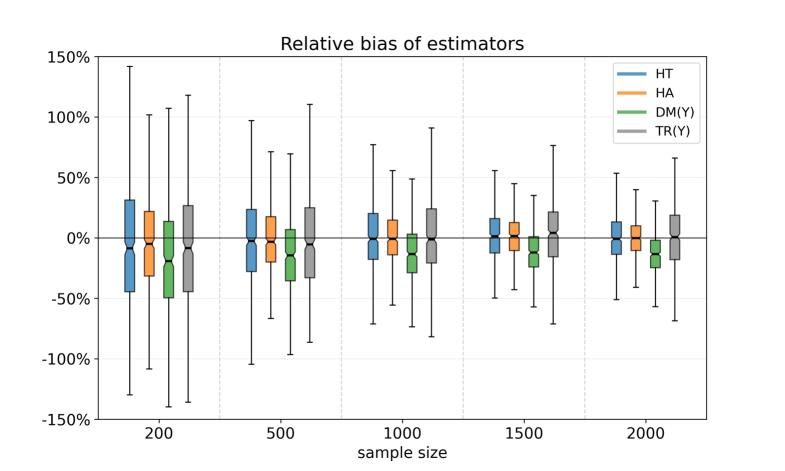
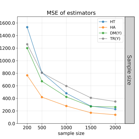
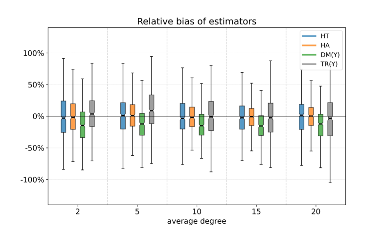
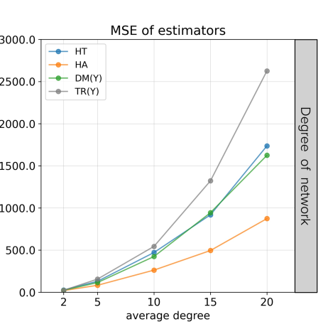
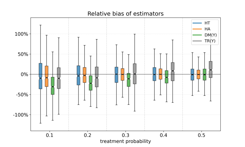
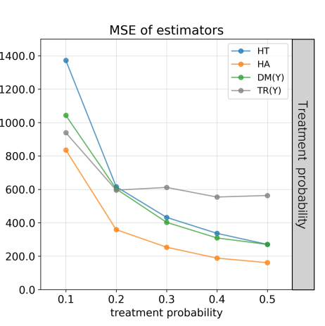
Figure S.8: (Lognormal setting) Relative bias and mean squared error of different estimators with varying sample size, degree of network and treatment probability.

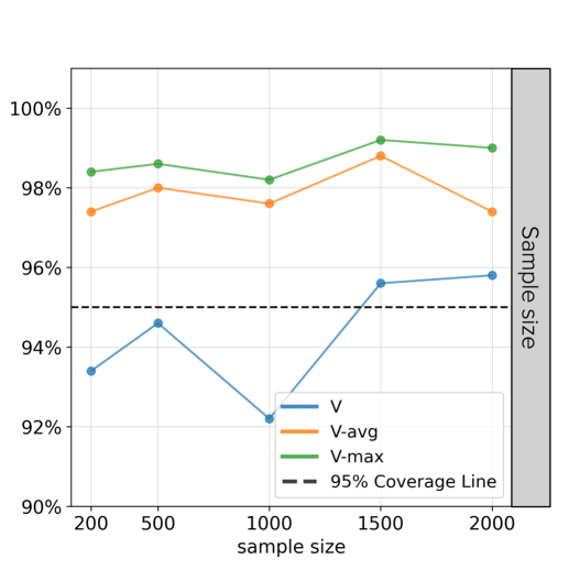
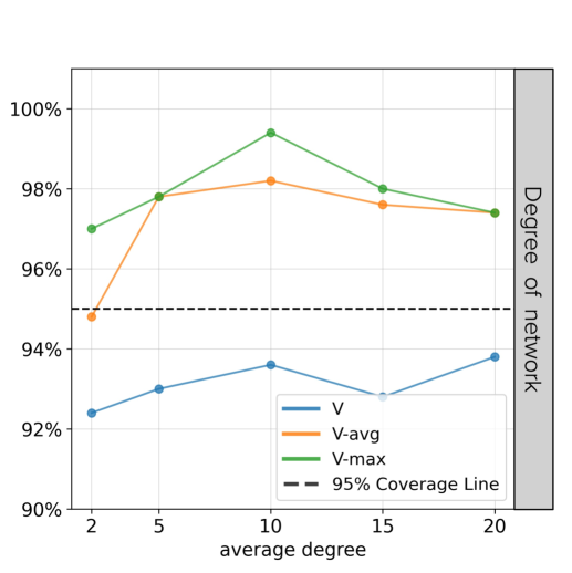
Figure S.9: (Lognormal setting) Coverage rate for the confidence interval based on different variance estimators with varying sample size, degree of network and treatment probability.

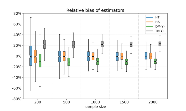
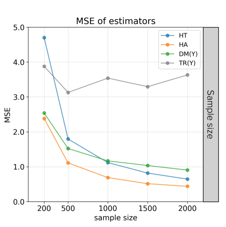
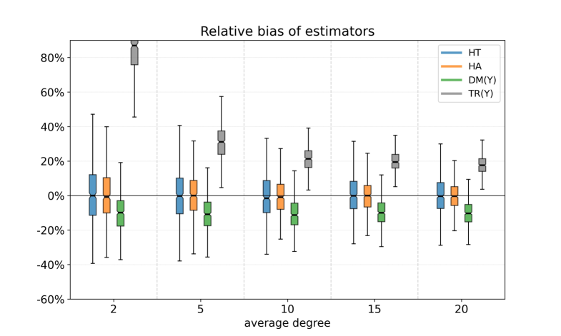
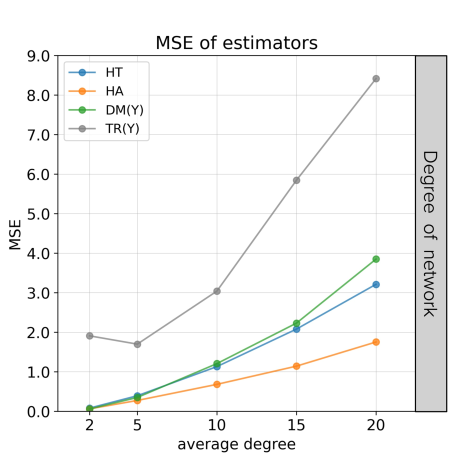
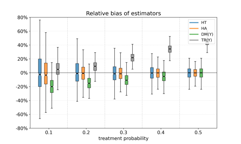
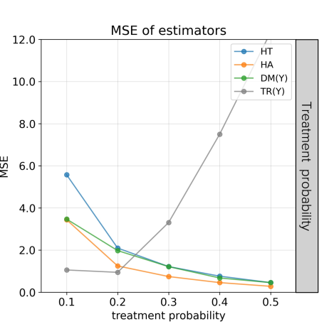
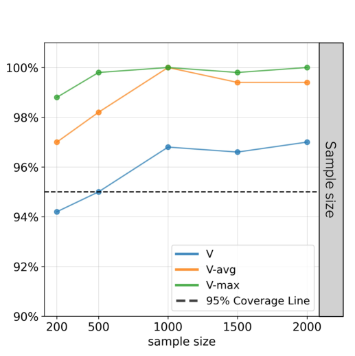
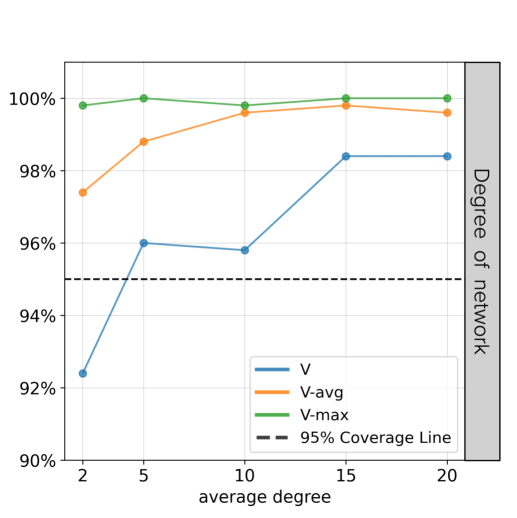
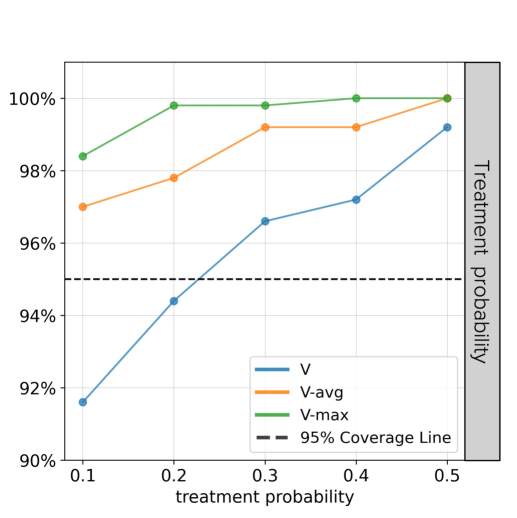
Figure S.10: (Binary setting) Relative bias and mean squared error of different estimators with varying sample size, degree of network and treatment probability.

Figure S.11: (Binary setting) Coverage rate for the confidence interval based on different variance estimators with varying sample size, degree of network and treatment probability.

References

• Albert and Barabási, (2002) Albert, R. and Barabási, A.-L. (2002). Statistical mechanics of complex networks. Reviews of Modern Physics, 74(1):47.
• Apicella et al., (2012) Apicella, C. L., Marlowe, F. W., Fowler, J. H., and Christakis, N. A. (2012). Social networks and cooperation in hunter-gatherers. Nature, 481(7382):497–501.
• Aronow and Samii, (2017) Aronow, P. M. and Samii, C. (2017). Estimating average causal effects under general interference, with application to a social network experiment. The Annals of Applied Statistics, 11(4):1912.
• Aronow et al., (2015) Aronow, P. M., Samii, C., and Assenova, V. A. (2015). Cluster–robust variance estimation for dyadic data. Political Analysis, 23(4):564–577.
• Bajari et al., (2023) Bajari, P., Burdick, B., Imbens, G. W., Masoero, L., McQueen, J., Richardson, T. S., and Rosen, I. M. (2023). Experimental design in marketplaces. Statistical Science, 38(3):458–476.
• Basse and Airoldi, (2018) Basse, G. W. and Airoldi, E. M. (2018). Limitations of design-based causal inference and a/b testing under arbitrary and network interference. Sociological Methodology, 48(1):136–151.
• Bhattacharya et al., (2020) Bhattacharya, R., Malinsky, D., and Shpitser, I. (2020). Causal inference under interference and network uncertainty. In Uncertainty in Artificial Intelligence, pages 1028–1038. PMLR.
• Bojinov and Shephard, (2019) Bojinov, I. and Shephard, N. (2019). Time series experiments and causal estimands: exact randomization tests and trading. Journal of the American Statistical Association, 114(528):1665–1682.
• Cameron and Miller, (2014) Cameron, A. C. and Miller, D. L. (2014). Robust inference for dyadic data. Unpublished manuscript, University of California-Davis, 15.
• Canen and Sugiura, (2024) Canen, N. and Sugiura, K. (2024). Inference in linear dyadic data models with network spillovers. Political Analysis, 32(3):311–328.
• Carlson et al., (2024) Carlson, J., Incerti, T., and Aronow, P. M. (2024). Dyadic clustering in international relations. Political Analysis, 32(2):186–198.
• Cattaneo et al., (2024) Cattaneo, M. D., Feng, Y., and Underwood, W. G. (2024). Uniform inference for kernel density estimators with dyadic data. Journal of the American Statistical Association, 119(548):2695–2708.
• Chiang and Tan, (2023) Chiang, H. D. and Tan, B. Y. (2023). Empirical likelihood and uniform convergence rates for dyadic kernel density estimation. Journal of Business & Economic Statistics, 41(3):906–914.
• Chin, (2019) Chin, A. (2019). Regression adjustments for estimating the global treatment effect in experiments with interference. Journal of Causal Inference, 7(2):20180026.
• Chung, (1997) Chung, F. R. (1997). Spectral graph theory, volume 92. American Mathematical Soc.
• Cortez-Rodriguez et al., (2022) Cortez-Rodriguez, M., Eichhorn, M., and Yu, C. L. (2022). Staggered rollout designs enable causal inference under interference without network knowledge. Advances in Neural Information Processing Systems, 35:7437–7449.
• Cortez-Rodriguez et al., (2023) Cortez-Rodriguez, M., Eichhorn, M., and Yu, C. L. (2023). Exploiting neighborhood interference with low-order interactions under unit randomized design. Journal of Causal Inference, 11(1):20220051.
• D’Amour and Airoldi, (2019) D’Amour, A. and Airoldi, E. M. (2019). Causal inference for dyadic outcomes in social network analysis.
• de Caen, (1998) de Caen, D. (1998). An upper bound on the sum of squares of degrees in a graph. Discrete Mathematics, 185(1-3):245–248.
• Eckles et al., (2016) Eckles, D., Karrer, B., and Ugander, J. (2016). Design and analysis of experiments in networks: Reducing bias from interference. Journal of Causal Inference, 5(1):20150021.
• Egami and Tchetgen Tchetgen, (2024) Egami, N. and Tchetgen Tchetgen, E. J. (2024). Identification and estimation of causal peer effects using double negative controls for unmeasured network confounding. Journal of the Royal Statistical Society Series B: Statistical Methodology, 86(2):487–511.
• Fafchamps and Gubert, (2007) Fafchamps, M. and Gubert, F. (2007). Risk sharing and network formation. American Economic Review, 97(2):75–79.
• Goldsmith-Pinkham and Imbens, (2013) Goldsmith-Pinkham, P. and Imbens, G. W. (2013). Social networks and the identification of peer effects. Journal of Business & Economic Statistics, 31(3):253–264.
• Graham et al., (2021) Graham, B. S., Niu, F., and Powell, J. L. (2021). Minimax risk and uniform convergence rates for nonparametric dyadic regression. Technical report, National Bureau of Economic Research.
• Graham et al., (2024) Graham, B. S., Niu, F., and Powell, J. L. (2024). Kernel density estimation for undirected dyadic data. Journal of Econometrics, 240(2):105336.
• Gupta et al., (2019) Gupta, S., Kohavi, R., Tang, D., Xu, Y., Andersen, R., Bakshy, E., Cardin, N., Chandran, S., Chen, N., Coey, D., et al. (2019). Top challenges from the first practical online controlled experiments summit. ACM SIGKDD Explorations Newsletter, 21(1):20–35.
• Hájek, (1960) Hájek, J. (1960). Limiting distributions in simple random sampling from a finite population. Publications of the Mathematical Institute of the Hungarian Academy of Sciences, 5:361–374.
• Han et al., (2024) Han, K., Basse, G., and Bojinov, I. (2024). Population interference in panel experiments. Journal of Econometrics, 238(1):105565.
• Han et al., (2023) Han, K., Li, S., Mao, J., and Wu, H. (2023). Detecting interference in online controlled experiments with increasing allocation. In Proceedings of the 29th ACM SIGKDD Conference on Knowledge Discovery and Data Mining, pages 661–672.
• Hu et al., (2022) Hu, Y., Li, S., and Wager, S. (2022). Average direct and indirect causal effects under interference. Biometrika, 109(4):1165–1172.
• Hudgens and Halloran, (2008) Hudgens, M. G. and Halloran, M. E. (2008). Toward Causal Inference With Interference. Journal of the American Statistical Association, 103(482):832–842.
• Hájek, (1971) Hájek, J. (1971). Comment on “an essay on the logical foundations of survey sampling, part one”. In The Foundations of Survey Sampling, (Eds., V.P. Godambe and D.A. Sprott), Holt, Rinehart, and Winston, Toronto, 236.
• Imbens and Rubin, (2015) Imbens, G. W. and Rubin, D. B. (2015). Causal Inference in Statistics, Social, and Biomedical Sciences. Cambridge University Press.
• Janson, (1988) Janson, S. (1988). Normal convergence by higher semiinvariants with applications to sums of dependent random variables and random graphs. The Annals of Probability, 16(1):305–312.
• Karrer et al., (2021) Karrer, B., Shi, L., Bhole, M., Goldman, M., Palmer, T., Gelman, C., Konutgan, M., and Sun, F. (2021). Network experimentation at scale. In Proceedings of the 27th ACM SIGKDD Conference on Knowledge Discovery and Data Mining, pages 3106–3116.
• Kohavi et al., (2020) Kohavi, R., Tang, D., and Xu, Y. (2020). Trustworthy Online Controlled Experiments: A Practical Guide to A/B Testing. Cambridge University Press.
• Leung, (2022) Leung, M. P. (2022). Causal inference under approximate neighborhood interference. Econometrica, 90(1):267–293.
• Leung, (2023) Leung, M. P. (2023). Network cluster-robust inference. Econometrica, 91(2):641–667.
• Li and Wager, (2022) Li, S. and Wager, S. (2022). Random graph asymptotics for treatment effect estimation under network interference. The Annals of Statistics, 50(4):2334–2358.
• Liu et al., (2016) Liu, L., Hudgens, M. G., and Becker-Dreps, S. (2016). On inverse probability-weighted estimators in the presence of interference. Biometrika, 103(4):829–842.
• Luke and Harris, (2007) Luke, D. A. and Harris, J. K. (2007). Network analysis in public health: history, methods, and applications. Annual Review of Public Health, 28(1):69–93.
• Luo et al., (2025) Luo, S., Shuai, K., Zhang, Y., Li, W., and He, Y. (2025). Identification and estimation of causal peer effects using instrumental variables. arXiv: 2504.05658.
• Manski, (2013) Manski, C. F. (2013). Identification of treatment response with social interactions. The Econometrics Journal, 16(1):1–23.
• Ogburn et al., (2020) Ogburn, E. L., Shpitser, I., and Lee, Y. (2020). Causal inference, social networks and chain graphs. Journal of the Royal Statistical Society Series A: Statistics in Society, 183:1659–1676.
• Ogburn et al., (2024) Ogburn, E. L., Sofrygin, O., Diaz, I., and Van der Laan, M. J. (2024). Causal inference for social network data. Journal of the American Statistical Association, 119(545):597–611.
• Portes and Rey, (2005) Portes, R. and Rey, H. (2005). The determinants of cross-border equity flows. Journal of International Economics, 65(2):269–296.
• Ross, (2011) Ross, N. (2011). Fundamentals of Stein’s method. Probability Surveys, 8:210–293.
• Rossi and Ahmed, (2015) Rossi, R. and Ahmed, N. (2015). The network data repository with interactive graph analytics and visualization. In Proceedings of the AAAI Conference on Artificial Intelligence, volume 29.
• Rubin, (1980) Rubin, D. B. (1980). Comment: Randomization analysis of experimental data: The Fisher randomization test. Journal of the American Statistical Association, 75(371):591–593.
• Saint-Jacques et al., (2019) Saint-Jacques, G., Varshney, M., Simpson, J., and Xu, Y. (2019). Using ego-clusters to measure network effects at linkedin. arXiv: 1903.08755.
• Särndal et al., (2003) Särndal, C.-E., Swensson, B., and Wretman, J. (2003). Model Assisted Survey Sampling. Springer Science & Business Media.
• Sävje, (2024) Sävje, F. (2024). Causal inference with misspecified exposure mappings: Separating definitions and assumptions. Biometrika, 111(1):1–15.
• Sävje et al., (2021) Sävje, F., Aronow, P., and Hudgens, M. (2021). Average treatment effects in the presence of unknown interference. The Annals of Statistics, 49(2):673.
• Shi and Ding, (2024) Shi, L. and Ding, P. (2024). Asymptotic theory for the quadratic assignment procedure. arXiv: 2411.00947.
• Tabord-Meehan, (2019) Tabord-Meehan, M. (2019). Inference with dyadic data: Asymptotic behavior of the dyadic-robust t-statistic. Journal of Business & Economic Statistics, 37(4):671–680.
• Tchetgen Tchetgen et al., (2021) Tchetgen Tchetgen, E. J., Fulcher, I. R., and Shpitser, I. (2021). Auto-g-computation of causal effects on a network. Journal of the American Statistical Association, 116(534):833–844.
• Thiyageswaran et al., (2024) Thiyageswaran, V., McCormick, T., and Brennan, J. (2024). Data-adaptive exposure thresholds for the Horvitz-Thompson estimator of the Average Treatment Effect in experiments with network interference. arXiv: 2405.15887.
• Traag et al., (2019) Traag, V. A., Waltman, L., and Van Eck, N. J. (2019). From Louvain to Leiden: guaranteeing well-connected communities. Scientific Reports, 9(1):1–12.
• Ugander et al., (2013) Ugander, J., Karrer, B., Backstrom, L., and Kleinberg, J. (2013). Graph cluster randomization: Network exposure to multiple universes. In Proceedings of the 19th ACM SIGKDD International Conference on Knowledge Discovery and Data Mining, pages 329–337.
• Ugander and Yin, (2023) Ugander, J. and Yin, H. (2023). Randomized graph cluster randomization. Journal of Causal Inference, 11(1):20220014.
• VanderWeele and Tchetgen, (2011) VanderWeele, T. J. and Tchetgen, E. J. T. (2011). Effect partitioning under interference in two-stage randomized vaccine trials. Statistics & Probability Letters, 81(7):861–869.
• Weng et al., (2024) Weng, C., Lei, X., and Si, N. (2024). Experimental design in one-sided matching platforms. Available at SSRN 4890353.
• Yu et al., (2022) Yu, C. L., Airoldi, E. M., Borgs, C., and Chayes, J. T. (2022). Estimating the total treatment effect in randomized experiments with unknown network structure. Proceedings of the National Academy of Sciences, 119(44):e2208975119.