Scalar perturbations to naked singularities of perfect fluid
Abstract.
In this paper, we study the instability of naked singularities arising in the Einstein equations coupled with isothermal perfect fluid. We show that the spherically symmetric self-similar naked singularities of this system, are unstable to trapped surface formation, under perturbations of an external massless scalar field. We viewed this as a toy model in studying the instability of these naked singularities under gravitational perturbations in the original Einstein–Euler system which is non-spherically symmetric.
1. Introduction
1.1. Previous works and a rough version of the main result
The weak cosmic censorship conjecture, one of the main conjectures in general relativity, asserts that naked singularities will not appear in gravitational collapse generically. The original statement proposed by Penrose [19] said that naked singularities will not appear in any cases, but soon examples of naked singularities in gravitational collapses were found in spherically symmetric massless scalar field collapsing (for example [3] and [7]). To insist on the validity of weak cosmic censorship, one hopes to prove that naked singularities are unstable under small perturbations, and therefore can only appear in very exceptional cases.
Soon after the discovery of naked singularities, Christodoulou [8] was able to show all possible naked singularities (not only those constructed in [7]) are unstable in the context of spherically symmetric solutions of Einstein–scalar field equations. Hence the weak cosmic censorship conjecture is true in this context, which is also studied in spherically symmetric collapse of charged scalar field by An–Tan [2]. In [15], we were able to give a constructive argument based on apriori estimates of Christodoulou’s proof in [8], instead of contradiction argument there, and show that [13] all possible spherically symmetric naked singularities are unstable to trapped surface formation under small gravitational perturbations (which must be outside spherically symmetric by Birkhoff Theorem). A recent work by An [1] showed that when the background naked singularity solutions are those constructed by Christodoulou in [7], which are continuously self-similar, fully anisotropic apparent horizon (not only trapped surfaces) can form under small gravitational perturbations in scale–critical norm.
In this paper we focus on the naked singularity model which is not of zero rest mass. The main difference from the before mentioned systems is that the matter field itself has a slower wave speed than light. Christodoulou [4] showed that spherically symmetric collapse of inhomogenuous dust cloud starting at rest would lead to stable formation of naked singularities, and more general cases were considered (see for example [22] and the references therein). This model may not be physical since pressure will not vanish at the final stage of a collapsing star. When the pressure comes in, the corresponding Einstein–Euler system is rather complicated, a general picture of gravitational collapse cannot be easily obtained. Nevertheless, naked singularities in Einstein–Euler were still found by Ori–Piran (see [18] and the references therein) by numerical method, assuming spherical symmetry and continuous self-similarity of the spacetime, and the rigorous proof of this existence was provided recently by Guo–Hazic–Jang [12].
It is then natural to ask about the instability of such kind of naked singularities, arising in gravitational collapse of (spherically symmetric) perfect fluid. At first glance, this problem is about the long time dynamic of self-gravitating relativistic fluid, which is not well-understood even in spherical symmetry in the literature. Nevertheless, we will try to study whether we can produce instability from the left hand side of the Einstein equations, i.e., the gravity part, as we are treating the whole Einstein–Euler system. The price is that we should go beyond spherical symmetry due to Birkhoff Theorem. To illustrate our main ideas, we will study the instability under spherically symmetric perturbations from an external massless real scalar field in this paper. As stated in Christodoulou’s survey [9], this is a good simplified model problem of Einstein’s theory of gravitation in case we impose spherical symmetry. In a further work [14], we will drop the scalar field and study the original Einstein–Euler system.
More precisely, we will study the following system of Einstein equations
| (1.1) |
where the energy momentum tensors of the coupled scalar field and perfect fluid are
and
here the equation of state for the fluid is the isothermal one: where is a constant, the square of sound speed. are the density, pressure and -velocity of the fluid, and . The spherically symmetric and continuously self-similar naked singularity solutions of isothermal perfect fluid (for example, those in [18, 12])) are solutions of (1.1) with . A rough version of the main result of this paper is the following.
Theorem 1.1.
The precise version is Theorem 1.2, presented in the Section 1.3. Although the naked singularities constructed in [18, 12] are the only known examples, we remark that our theorem (see precise version below) applies to much wider class of spherically symmetric naked singularity solutions that could be far from being continuously self-similar.
1.2. The geometry of the past null cone of the singularity
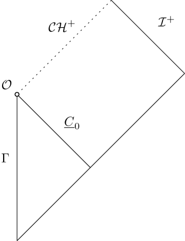
In the proof of naked singularity instability before, the most important feature is the geometry of the past null cone. Suppose that is the past null cone of the singularity (see Figure 1), in the case of Einstein–scalar field system, is a singularity (of solution, see [6]) if and only if the mass ratio when approaching from the past of . This implies the integral along , which is a measurement of the blue-shift of light received by ,
| (1.2) |
is infinite. Christodoulou’s proof in [8] makes essential use of this quantity. In our new proof [15], we observed that the divergence of (1.2) implies that the lapse function of a double null foliation around , with on , tends to zero as approaching along , which is one of the most important ingredients of our proof in [15].
We are thus led to see whether other naked singularity solutions we are interested in verify the same condition. In order to check the behavior of along , we turn to the Raychaudhuri equation along incoming direction, the equation (2.2) in the section below. Together with the gauge choice
| (1.3) |
along , we have and hence (2.2) becomes
| (1.4) |
The question then reduces to see whether the integral of the right hand side on diverges. It turns out that it is related to the so-called strength of the singularity, introduced by Tipler in [23], which was widely investigated in physics literature. Roughly speaking, a singularity is called a strong curvature singularity (along some causal geodesic approaching it, say ), if the volume form generated by Jacobi fields along tends to zero. A sufficient condition for the singularity being strong along , derived in [11], is
| (1.5) |
where is the affine parameter of , and represents the singularity. It had been checked in [18] that in the naked singularity solutions considered there, condition (1.5) is true along radial null geodesics emerge from and terminate at . It can then be seen from equation (1.4) that . This is because if , then it has a positive lower bound since it is monotonely decreasing by negativity of the right hand side of (1.4). Then because , we know and . Therefore (1.5) implies that the right hand side of (1.4) looks like , then by integrating (1.4), we have , a contradiction. It should be noted that is simply the volume form of the -dimensional quotient spacetime generated by and .
In fact, we have a more direct argument to see , and moreover an accurate rate. Recall that a spherically symmetric spacetime is called (continuously) self-similar, if there exists a conformal Killing field such that
and in particular , where is the Lorentzian metric induced on the -dimensional quotient spacetime, is the area radius of the orbit spheres. Let us assume that, which is true as checked in [18], , the past null cone of the singularity , is invariant under the flow generated by 111In fact, the meaning of the term “the past null cone of the singularity ” should be clarified since is not included in the spacetime. However, we can simply take to be the level set of self-similar parameter that is null, if it exists.. Then on we have . The self-similarity also implies that , and hence . Restricted on , we will have
| (1.6) |
Plugging in (1.4), the right hand side then looks like , and then
| (1.7) |
Note that this argument applies to all kinds of Einstein–matter field systems since we only use the invariance of the Ricci tensor under self-similarity. It also applies in vacuum if we simply replace the Ricci tensor (which vanishes in vacuum) by the shear tensor (see naked singularity solutions in vacuum constructed in [20]). Of course, for a particular matter field system, the variables of matter field should also obey self-similarity. For example, in self-similar Einstein–Euler system with isothermal perfect fluid under consideration, the fluid variables verify on that
| (1.8) |
These conditions are of course consistent with (1.6).
1.3. The precise statement of the main result and comments
Now we are going to give the precise statement we want to prove. The same to before, we consider a double null characteristic problem of the system (1.1), with initial data given on two intersecting null cone, and , where is the past null cone of the singularity , and is the outgoing null cone whose intersection with is the sphere .
The data on is induced from the naked singularity solutions in [18, 12], satisfies (1.8). In fact, our method is robust and we will allow and being only bounded above and below by positive constants, together with their derivatives being bounded. In this case, on is bounded above and below by positive constants, and hence
| (1.9) |
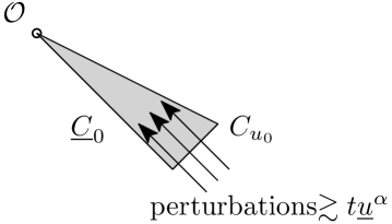
holds with , instead of (1.7). In the proof, we only need the upper bound of . We remark that in our previous works [15, 13] on Einstein–scalar field system, only is needed, no other informations about and even no informations on the data on are needed. The data on is spherically symmetric, consists of the fluid variables and the scalar field , or more precisely, the derivative along . For we only consider smooth solution and vanishes on , is required to be smooth up to where . The main result of this paper is the following (also see Figure 2).
Theorem 1.2.
Consider double null characteristic problem of the system (1.1) in spherical symmetry. Suppose that on the incoming null cone , endowed with a parameter , and there is an such that on ,
We also assume the Hawking mass and all spherical sections of are not trapped222If there is a trapped section on , then the vertex singularity is not naked.. Then there is a one-parameter family of initial (for sufficiently small) on , endowed with a parameter such that
in topology (as a function of ), for some depending on , and the maximal future development of such initial data has a closed trapped surface preceding for .
Moreover, the perturbations are generic in the following sense: the set of all data on such that there is a closed trapped surface preceding in its maximal future development, contains an open set of which zero data (leading to naked singularity solution) is its limit point in topology.
Remark 1.1.
The non-negativity of the mass on holds true in naked singularity solutions, which admit a regular central line. In fact, in this double null setting, our proof also applies to the case when is bounded below by a negative constant, in which case the solution cannot admit a regular central line.
The proof of this theorem contains the following two main ingredients:
-
•
The instability mechanism: This part is similar to the previous work [15]. Roughly speaking, once we can prove that in the region , all dimensionless variables of the system (such as expansions of null cones , derivatives of scalar field and fluid variables ) are suitably bounded (in spherical symmetry, this can be done by method of characteristic), then by integrating the wave equation (2.9), that is,
along direction, we expect that on for is as large as its value on the initial null cone . Then the Raychaudhuri equation along , equation (2.5) written in the following form
tells us that the right hand side becomes sufficiently large when because . So can become negative when integrating along when is sufficiently small. A slight difference from [15] is that we don’t have a criterion of trapped surface formation like that in [5], which is crucial in Christodoulou’s original proof [8]. Nevertheless, we can still prove trapped surface formation in a direct way.
-
•
The estimates for fluid variables: According to our setting (the perturbations are added exterior to the past null cone of ), perturbations from fluid cannot produce trapped surface around the singularity since it has slower wave speed than light, then the past sound cone of points near will not intersect . On the other hand, since the background geometry changes a lot (trapped surfaces form due to perturbations of scalar field), we must carefully show that, in the region we are working in, the fluid variables still behave well (for example, shocks will not form) and obey the self-similar estimates which are needed in the previous ingredient. The main reason why this works is that solving the Euler equations in the region is a local problem (we will prove that both characteristic curves have length ), while solving Einstein–scalar field equations is semi-global.
We close this section by some final remarks.
Remark 1.2.
Though the perturbations are measured in , we only consider smooth solutions to avoid details in establishing local–wellposedness of weak solution of the system (1.1), which is possible because we don’t need to close the apriori estimates. Local wellposedness of smooth solutions of spherically symmetric Einstein–Euler system in double null setting was established in [12]. If passing to weak solutions, the perturbations looks like when and the apparent horizon emerging from the singularity can be found, just as the original Einstein–scalar field system. Smooth perturbations are obtained by cutting off.
Remark 1.3.
In the current paper, the reason why we can establish instability (which is better than all previous related works) is rooted in the quantitative behavior (1.9), in which only the upper bound is needed. But it should be noted that the Hölder index depends on particular background naked singularity solution. Finding the optimal Hölder index is an interesting problem. See more detailed discussions in [21].
Remark 1.4.
We expect that our method apply to most matter fields that have a slower sound speed than light, showing that the corresponding naked singularity solutions, when the singularities are strong, are unstable to trapped surface formation under gravitational perturbations. This will support a conjecture formulated by Newman [17] that naked singularities appearing in gravitational collapse are in some sense gravitationally weak. Note that the naked singularity solutions of spherically symmetric inhomogeneous dust collapse () constructed by Christodoulou [4] has a weak naked singularity along radial past and future null geodesics [16]. There exist some exceptional choices of initial configurations of spherically symmetric inhomogeneous dust collapse such that the resulting naked singularities are strong along past and future null geodesics (see for example [22]), in which case our argument can also apply. We can also consider the case of stiff fluid (), even though we don’t have a precise example of naked singularity solution in this case. But in this case, the existence of the fluid part becomes semi-global and then it raises new difficulties. Moreover, because the sound speed of stiff fluid is the same to the light speed, one may hope to show instability without external scalar field.
Acknowledgement
This work is supported by National Key R&D Program of China (No. 2022YFA1005400), NSFC (12326602, 12141106).
2. Double null coordinate and equations
2.1. Double null coordinate
In a spherically symmetric spacetime, let us introduce the double null coordinate , where , are optical functions, which means that their level sets and are incoming and outgoing null cones respectively, invariant under the action representing spherical symmetry. We denote , which is an orbit sphere. In the quotient spacetime, and are then incoming and outgoing null lines respectively. We denote
to be the coordinate vector fields, and the lapse function is defined by
The metric then takes the following form
where the area radius function is defined by
and is the standard metric of the unit sphere.
2.2. Equations
The estimates are done using the null structure equations. In spherical symmetric case, the non-vanishing components of connections are
where and are the restrictions on the orbit spheres of the Lie derivatives along and . When applying on functions, and are simply the ordinary derivatives. Here and are the null expansions relative to the normalized pair of null vectors , . Then null structure equations are333These equations can be derived as in [10], in which the equations without any symmetries in vacuum are obtained. One only needs to carefully bring back the Ricci tensor. Readers can also see [5] in which the notations are slightly different.
| (2.1) | ||||
| (2.2) | ||||
| (2.3) | ||||
| (2.4) |
Here represents the trace of taken on the orbit spheres.
For the Einstein-scalar field-Euler system (1.1), the energy momentum tensor reads
where
and
From (1.1), we then have
Plugging in the above expressions of the Ricci tensor, equations (2.1)-(2.4) become:
| (2.5) | ||||
| (2.6) | ||||
| (2.7) | ||||
| (2.8) |
We turn to the equations satisfied the matter fields. The scalar field obeys the wave equation
and the fluid variables obey the relativistic Euler equations
with , where
is the acoustical metric.
We should decompose the wave and Euler equations in double null coordinate. Let us introduce
then the wave equation can be written in the following form:
| (2.9) | ||||
| (2.10) |
These two equations are in fact the same equation. For fluid variables, we denote
where is such that . We then have
We have and since is a future directed unit timelike vector.
We should write the relativistic Euler equations in the form allowing us to use the method of characteristics.
Lemma 2.1.
A regular solution of the relativistic Euler equations verify the following equations whenever :
| (2.11) |
| (2.12) |
where are the outgoing and incoming future directed acoustical-null vectors () of unit length:
| (2.13) |
Remark 2.1.
The crucial fact is that the right hand sides contain no derivatives of . The expressions (2.13) of can be seen in the course of the proof, or directly obtained by the method of undetermined coefficients by and .
Proof.
These equations can also be found in [12] written in different notations. For completeness, we outline the computations here. The Euler equations are simply the conservation law of the energy momentum tensor:
Using the frame where are spherical, its components are
| (2.14) |
where is the round metric of radius induced on spherical sections. By direct checking, we have the following formulas of connections:
and the only non-vanishing components of :
where we use in evaluating . Then (2.14) becomes
Dividing the first by and the second by we have (using again )
| (2.15) |
where is to be determined. We then multiply the second equation by and then compare the coefficient of the second term, that is,
| (2.16) |
Then we can sum up two equations to obtain equations for and . The positive root of (2.16) is simply , as indicated in (2.11), (2.12). The negative root of (2.16) leads to the same equations.
3. A priori estimates
We begin to prove Theorem 1.2. In this section, we are going to derive a priori estimates. Recall that we consider double null characteristic problem of Einstein–scalar field-Euler system (1.1) in spherical symmetry. The incoming cone is endowed with the parameter , where is one of the optical functions in the spacetime we consider, and also on . We denote
to be the restriction of and on . Note that since is decreasing when by (1.4) and energy condition, by rescaling , we can set and then for . Note also that we have , which is equivalent to the positivity of the Hawking mass (on we have ) and since has no closed trapped surfaces on it. In the following, we use
to denote for some constant , depending only on .
Theorem 3.1.
There exists a constant depending on such that the following statement is true. Let be such that
Then for any such that
| (3.1) |
the following estimates holds for ,
| (3.2) |
| (3.3) | ||||
| (3.4) | ||||
| (3.5) | ||||
| (3.6) |
| (3.7) | ||||
| (3.8) | ||||
| (3.9) | ||||
| (3.10) |
Proof.
It suffices to prove the estimates under the bootstrap assumptions
| (3.11) | ||||
| (3.12) | ||||
| (3.13) | ||||
| (3.14) |
| (3.15) | ||||
| (3.16) |
where is small ( is sufficient) and is sufficiently large and to be determined.
From the equation , using (3.1) and the bound (3.13), we have
If is sufficiently large, and the estimate (3.2) for follows. Here we use the fact that and .
To estimate , note that if is sufficiently large,
| (3.17) |
where we have used (3.1), (3.2) for and . Then from , we have
Then if is sufficiently large, the estimate (3.2) for holds.
Next we estimate the matter fields. From the wave equation , using (3.1), (3.15) and (3.17),
and from the other version of the wave equation , using the above estimate,
where we have used
| (3.18) |
Next we turn to the estimates for the fluid variables. For each , let be the integral curve of passing through , with (The existence of such a point can be argued as follows: For an inextendible timelike curve with unit tangent, it must intersect the past boundary of a global hyperbolic spacetime). Note that for different (those on the same integral curve), can be the same. We denote be the parameter of at .
In order to estimate the fluid variables, we need to estimate the length of in the spacetime region that we consider, and the variation of and along . We begin by assuming that, for any ,
| (3.19) |
which is an estimate of the variation of the function along the integral curves of . The the equation (2.6) restricted on (where and hence ) reads
| (3.20) |
Particularly, we can see again this implies that is monotonically decreasing along . On we have , then by integrating it from to , we have
where the last inequality is by (3.19). This implies that, for ,
By the monotonicity of , the above can be replaced by for any , then using (3.2) we have
| (3.21) |
for . This is the variation of along .
Then we are going to estimate , representing the length of . Note that
by integrating the right hand side along from to , we have
where we have used (3.16) and and (3.21). This implies that
| (3.22) |
Now we are going to retrieve the estimate (3.19). From
the difference of the values of at the starting point and ending point of is estimated by
where we have used (3.16) and (3.22) in the first inequality and (3.1) in the second inequality (Note that , and ). We also use . If is chosen sufficiently large, we then have, for ,
which improves the estimate (3.19). This implies that (3.19) is in fact true for each with replaced by and hence the subsequent estimates are also true. Moreover, we have
| (3.23) |
for . The estimates (3.21) and (3.23) together tells us that when integrating along , we can simply replace and in the integrants by their values at the end points .
We introduce an additional bootstrap assumption
| (3.24) |
for , , which guarantees that throughout the spacetime region we consider. Also, since , we can refer to the Euler equations (2.11), (2.12), denoting the right hand sides by :
| (3.25) |
| (3.26) |
Using (3.14), (3.16) and (3.2), (3.17), (3.18), the right hand sides of the above two equations are bounded by
Using (3.22) and (3.1), we find
By choosing sufficiently large, we have
By integrating the Euler equations, we have
and
which implies that
and
By these two relations, we have
where we have used the initial bound of and (3.23). The same procedure gives the same bound for :
which improves (3.24). This implies that the bound (3.9) is true without assuming (3.24). Similarly, we have
and the same for . So we have proved (3.10). In particular, we can drop the factor in (3.22), by using the bound (3.10) and go through the estimates there again. That is, it holds that
| (3.27) |
which is an estimate of the length of inside the spacetime region we consider.
Finally we consider the connection coefficients. From the equation (2.5), and the bounds (3.2), (3.7), (3.9), (3.10), we have
This proves (3.3). From the equation (2.7), and the bounds (3.2), (3.17), (3.18) and (3.9), we have
This proves (3.4). By (3.2), (3.17), (3.18), (3.7), (3.8) and (3.9), the right hand side of equation (2.8) is estimated by
where in the last inequality we use (3.1). Then by the initial bound of on , the estimate (3.5) of follows by integrating above bound relative to . For , we will need its initial bound on :
where we use the equation (3.20) on . Then by (2.8), we have
We have closed the estimates of the geometric quantities , derivatives of the scalar function and the fluid variables in the region for satisfying (3.1). To construct a regular solution, we also need to consider the first derivatives of the fluid variables.
Theorem 3.2.
Remark 3.1.
Here is geodesic. Recalling , from the relation , in fact we have . We estimate derivative of instead of simply because estimating the latter one will involve an estimate of , which we want to avoid.
Remark 3.2.
Proof.
We will commute with the Euler equations. To avoid estimating , we rewrite the Euler equation as
| (3.30) |
| (3.31) |
The left hand sides are about and instead of and , and instead of appears at the right hand sides. A simple way to derive these equations is taking the “conjugates” of (3.25) and (3.26), that is, changing “” to “” and vice versa, “” to “” and “” to “”. One can also use directly the expressions of in (2.13), the original Euler equations (3.25), (3.26) and write and .
Commuting , we have
| (3.32) |
| (3.33) |
By direct computation, recalling (2.13) and the relation , we have
| (3.34) |
Using (2.13) again and , we have
Plugging in the equations (3.30), (3.31), the equations (3.32), (3.33) become
| (3.35) |
| (3.36) |
where are defined in (3.30), (3.31) and
We only need to prove (3.29) under the bootstrap assumptions:
| (3.37) |
Using the estimates derived in Theorem 3.1, and (3.17), (3.18), we know
And then by (3.6), (3.10) and (3.37), we have
| (3.38) |
and
| (3.39) |
By equations (2.7) and (2.8), and using (3.1), (3.17), (3.18) and the estimates derived in Theorem 3.1, we have
furthermore, by (2.6) and the relation , we have
and by (3.37), we have
By combining these estimates, we have
| (3.40) |
Using (3.27), the estimate (3.39) integrating along gives
where we have used (3.28) and (3.1) in the last inequality. By choosing sufficiently large, we will have
| (3.41) |
By integrating the estimates (3.38) and (3.40) along , we have
| (3.42) |
where we have used (3.1) in the last inequality. (3.28) is not needed here because the inhomogeneous term is linear to the first order derivative.
The bounds for higher order derivatives of and can be estimated by commuting more and to the equations. The resulting equations are linear relative to the higher order derivatives, so the estimates can be derived directly in terms of the corresponding bounds on , in the region for satisfies (3.1) and (3.28). The higher order bounds need not to have a self-similar form as those in Theorem 3.1 and 3.2. Then a regular solution of the system (1.1) in double null coordinates in this region can be constructed by standard argument (see for example [12] without scalar field).
4. Formation of trapped surfaces and instability
In the last section we will find the trapped surface formed in the solution by requiring that the initial scalar field on satisfies certain lower bound condition.
Theorem 4.1.
Proof.
then (3.1) and (3.28) hold, and hence the solution exists and all estimates of Theorems 3.1, 3.2 hold.
From the wave equation,
we have, for some universal constant , using (3.8) and (3.17),
Thus we have
and then
By integrating relative to , we have
where we have used (4.4) at the second step and set .
From the equation (2.5),
we have, on , using (3.2) and (4.1),
since , we have , which completes the proof.
We finally turn to the proof of Theorem 1.2.
Proof of Theorem 1.2.
It is easy to see there are depending on and in Theorem 1.2 such that the assumptions of bounds for initial data on in Theorems 3.1, 3.2 hold, and the bounds for initial data on are trivially true, by choosing possibly larger and . Therefore we can apply Theorem 4.1. We will construct verifying all requirements in Theorem 4.1.
From the assumptions of Theorem 1.2, we can find depending on and such that the right hand side of (3.20), the restriction of (2.6) on , is bounded from above by . We therefore have, for ,
So we will have, for some depending on and ,
Set . Note that under the relation (4.4), the condition (4.3) becomes
for some constant . Therefore, given any , and any sufficiently small, we can find depending on various constants, including , such that
| (4.5) |
and defined by as in (4.4) verifies (4.2). We moreover choose a such that
Now we may choose a smooth such that
Note that for all small , can be chosen independent of . Then such verifies all requirements in Theorem 4.1 and hence is a closed trapped surface in the corresponding maximal development.
To show the last statement in Theorem 1.2, given any such constructed above, let be a smooth function in be such that and
Then in particular we have
we then have
for sufficiently small. By choosing smaller such that the number is replaced by in (4.5), we then have
Then if we set another initial data , it still verifies all requirement in Theorem 4.1 and hence a close trapped surface still forms. Then the open set in the last statement in Theorem 1.2 can be chosen as
which is open as a union of open sets. The proof is then completed.
References
- [1] X. An, Naked Singularity Censoring with Anisotropic Apparent Horizon, arXiv:2401.02003.
- [2] X. An, H. K. Tan, A Proof of Weak Cosmic Censorship Conjecture for the Spherically Symmetric Einstein-Maxwell-Charged Scalar Field System, arXiv:2402.16250
- [3] M.W. Choptuik, Universality and scaling in gravitational collapse of a massless scalar field, Phys. Rev. Lett., 70, 9–12, (1993).
- [4] D. Christodoulou, Violation of cosmic censorship in the gravitational collapse of a dust cloud, Commun. Math. Phys. 93, 171–195 (1984).
- [5] D. Christodoulou, The formation of black holes and singularities in spherically symmetric gravitational collapse, Communications on Pure and Applied Mathematics 44, no. 3 (1991): 339-373.
- [6] D. Christodoulou, Bounded variation solutions of the spherically symmetric einstein-scalar field equations, Communications on Pure and Applied Mathematics 46, no. 8 (1993): 1131-1220.
- [7] D. Christodoulou, Examples of Naked Singularity Formation in the Gravitational Collapse of a Scalar Field, Annals of Mathematics, (1994) 140(3), 607–653.
- [8] D. Christodoulou, The instability of naked singularities in the gravitational collapse of a scalar field, Ann. of Math. 149, 183-217 (1999).
- [9] D. Christodoulou, On the global initial value problem and the issue of singularities, Class. Quantum Grav. (1999) 16 A23.
- [10] D. Christodoulou, The Formation of Black Holes in General Relativity, Monographs in Mathematics, European Mathematical Soc. 2009.
- [11] C.J.S. Clarke, A. Królak, Conditions for the occurence of strong curvature singularities, Journal of Geometry and Physics, Volume 2, Issue 2, 127–142, 1985.
- [12] Y. Guo, M. Hadzic, M., J. Jang, Naked Singularities in the Einstein-Euler System, Ann. PDE 9, 4 (2023).
- [13] J. Li, and J. Liu Instability of spherical naked singularities of a scalar field under gravitational perturbations, Journal of Differential Geometry, 120(1): 97-197, 2022.
- [14] J. Li and X. P. Zhu, in preparation.
- [15] J. Liu and J. Li, A robust proof of the instability of naked singularities of a scalar field in spherical symmetry, Comm. Math. Phys. 363 (2018), no. 2, 561–578
- [16] R. P. Newman, Strengths of naked singularities in Tolman-Bondi spacetimes, Classical and Quantum Gravity, 3, 527-539, 1986.
- [17] R. P. Newman, Cosmic Censorship and the Strengths of Singularities. In: Bergmann, P.G., De Sabbata, V. (eds) Topological Properties and Global Structure of Space-Time. NATO ASI Series. Springer, Boston, MA, 1986.
- [18] A. Ori, T. Piran, Naked singularities and other features of self-similar general-relativistic gravitational collapse, Phys. Rev. D 42, 1068, 1990
- [19] R. Penrose, Gravitational collapse: the role of general relativity, Noovo Cimento 1, 252 - 276 (1969).
- [20] I. Rodnianski, Y. Shlapentokh-Rothman, Naked singularities for the Einstein vacuum equations: The exterior solution, Ann. Math., 198 (2023), 1, 231-391
- [21] J. Singh, High regularity waves on self-similar naked singularity interiors: decay and the role of blue-shift, arXiv: 2402.00062
- [22] T. P. Singh, P. S. Joshi, The final fate of spherical inhomogeneous dust collapse, Class. Quantum Grav. 13 559, 1996
- [23] F. J. Tipler, Singularities in conformally flat spacetimes, Physics Letters A, 64, 1, 8–10, 1977