Practical estimation of the optimal classification error
with soft labels and calibration

Abstract

While the performance of machine learning systems has experienced significant improvement in recent years, relatively little attention has been paid to the fundamental question: to what extent can we improve our models? This paper provides a means of answering this question in the setting of binary classification, which is practical and theoretically supported. We extend a previous work that utilizes soft labels for estimating the Bayes error, the optimal error rate, in two important ways. First, we theoretically investigate the properties of the bias of the hard-label-based estimator discussed in the original work. We reveal that the decay rate of the bias is adaptive to how well the two class-conditional distributions are separated, and it can decay significantly faster than the previous result suggested as the number of hard labels per instance grows. Second, we tackle a more challenging problem setting: estimation with corrupted soft labels. One might be tempted to use calibrated soft labels instead of clean ones. However, we reveal that calibration guarantee is not enough, that is, even perfectly calibrated soft labels can result in a substantially inaccurate estimate. Then, we show that isotonic calibration can provide a statistically consistent estimator under an assumption weaker than that of the previous work. Our method is instance-free, i.e., we do not assume access to any input instances. This feature allows it to be adopted in practical scenarios where the instances are not available due to privacy issues. Experiments with synthetic and real-world datasets show the validity of our methods and theory. The code is available at https://github.com/RyotaUshio/bayes-error-estimation.

1 Introduction

It is a common practice in the field of machine learning research to assess the performance of a newly proposed algorithm using one or more metrics and compare them to the previous state-of-the-art (SOTA) performance to show its effectiveness (Neu, 2024; Int, 2025a, b). In classification, arguably the most common one is the error rate, i.e., the expected frequency of misclassification for future data.

While the SOTA performance continues to improve for a wide range of benchmarks over time, there is a limit on the prediction performance that any machine learning model can achieve, which is determined by the underlying data distribution. It is important to know this limit, or the best achievable performance. For example, if the current SOTA performance is close enough to the limit, there is no point in seeking further improvement. It is not only wasteful in terms of time and financial resources but also harmful to the environment, since large-scale machine learning models are notorious for their high energy consumption (Strubell et al., 2020; Luccioni et al., 2023). Knowing the best possible performance also provides a practical check for test-set overfitting (Recht et al., 2018; Ishida et al., 2023): if a model’s score on the test set approaches or even exceeds the upper bound, it may be a signal of the model directly training on the test set.

In classification, the best achievable error rate for a given data distribution is called the Bayes error, and the estimation of the Bayes error has a rich history of research (Fukunaga and Hostetler, 1975; Devijver, 1985; Berisha et al., 2014; Moon et al., 2018; Noshad et al., 2019; Theisen et al., 2021; Ishida et al., 2023; Jeong et al., 2023). In the case of binary classification, the existing approaches can be roughly categorized into two groups: the majority of estimation from instance-label pairs $(x_{1},y_{1}),\dots,(x_{n},y_{n})\in\mathcal{X}\times\left\{{0,1}\right\}$ (Fukunaga and Hostetler, 1975; Devijver, 1985; Berisha et al., 2014; Moon et al., 2018; Noshad et al., 2019; Theisen et al., 2021), where $\mathcal{X}$ is the space of instances, and the recently proposed methods of estimation from soft labels $\eta_{1},\dots,\eta_{n}\in[0,1]$ (Ishida et al., 2023; Jeong et al., 2023). A soft label is a special type of supervision that represents the posterior class probability $\eta_{i}\coloneqq\mathbb{P}(y=1\mid x=x_{i}),\ i\in\left\{{1,\dots,n}\right\}$, and it quantifies the uncertainty of class labels associated with each instance $x_{i}$. The strength of the methods proposed in (Ishida et al., 2023; Jeong et al., 2023) based on soft labels is that they are instance-free, i.e., they do not require access to the instances $\left\{{x_{i}}\right\}_{i=1}^{n}$. Since the instances themselves are not used for estimation, these methods do not suffer from the curse of dimensionality even when dealing with very high-dimensional data. Moreover, the instance-free property is practically valuable since it makes the methods easy to apply to real-world problems, such as medical diagnoses, where the instances are often inaccessible due to privacy concerns. However, these methods have a crucial limitation: they assume that we have direct access to clean soft labels $\eta_{i}=\mathbb{P}(y=1\mid x=x_{i})$, which only an oracle would know. Ishida et al. (2023) also discussed a scenario where each soft label $\eta_{i}$ is approximated by an average $\widehat{\eta}_{i}=\frac{1}{m}\sum_{j=1}^{m}y_{i}^{(j)}$ of $m$ hard labels $y_{i}^{(1)},\dots,y_{i}^{(m)}$ per instance. They showed that, for a fixed number $n$ of samples, the bias of the resulting estimator approaches zero as $m$ tends to infinity. However, their bound on the bias is prohibitively large for practical values of $m$, and thus the theoretical guarantee for this estimator is weak.

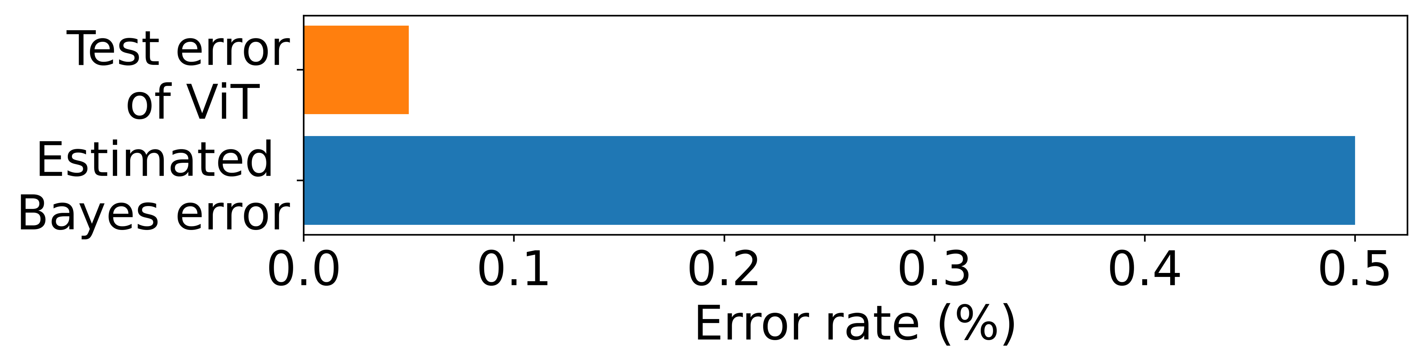
Figure 1: The Bayes error estimated with the method of Ishida et al. (2023) is larger than the test error of a Vision Transformer (Dosovitskiy et al., 2021).

Another issue is labeling distribution shift. For example, whereas the images in the original CIFAR-10 dataset (C-10) (Krizhevsky, 2009) can be regarded as though they were annotated before they were downscaled, the images in the CIFAR-10H dataset (C-10H) (Peterson et al., 2019) were annotated after downscaling, making the task more challenging and thus increasing label uncertainty. Given that the Bayes error can be interpreted as the average label uncertainty, we will get an unreasonably high estimate of the Bayes error if we just plug the soft labels in C-10H into their estimator, as shown in Figure˜1. In general, a similar issue can arise due to subjectivity of human soft labelers, or the bias of using large language models (LLMs) as annotators (Gilardi et al., 2023; Tjuatja et al., 2024). Recent work has explored a range of techniques to obtain soft labels and confidence scores from LLMs, but constructing a high-quality soft label remains to be a challenge (Xie et al., 2024; Kadavath et al., 2022; Argyle et al., 2023). This distortion issue due to the distribution shift was also mentioned by Ishida et al. (2023), but no solution was shown in their paper.

Contribution of this paper We extend the previous work by Ishida et al. (2023) that utilizes soft labels for estimating the Bayes error, the optimal error rate, in two important ways.

First, we deepen the theoretical understanding of the bias of the hard-label-based estimator discussed in the original work. Specifically, we show that the decay speed of the bias depends on how well the two class-conditional distributions are separated, and it can approach zero significantly faster than the previous result suggested as the number $m$ of hard labels per instance grows. On the journey of our proof, we extend an existing result (Liao and Berg, 2019) to tailor a generalized version of the classical Jensen inequality, which might deserve an independent interest.

Second, we discuss a new, more challenging problem of estimation from corrupted soft labels. In this scenario, we are given a distorted version of the clean soft labels. The distortion can arise from a shifted labeling distribution or subjectivity of human/LLM soft labelers. It reflects many real-world problems including the estimation of best achievable performances for benchmark datasets and estimation from soft labels obtained from subjective confidence. One might be tempted to use calibrated soft labels in place of clean ones. However, we reveal that calibration guarantee is not enough, i.e., even perfectly calibrated soft labels can result in a substantially inaccurate Bayes error estimate, which highlights the importance of choosing appropriate calibration algorithms. Then, we show that a classical calibration algorithm called isotonic calibration (Zadrozny and Elkan, 2002) can provide a statistically consistent estimator as long as the original soft labels are correctly ordered.

2 Fine-grained analysis of the bias

We first explain the preliminaries for this section and then present our main results.

2.1 Preliminaries

Formulation and notations  Let $\mathcal{X}\subset\mathbb{R}^{d}$ and $\mathcal{Y}$ be the spaces of instances and output labels, respectively. In this paper, we confine ourselves to binary classification problems and thus we set $\mathcal{Y}=\left\{{0,1}\right\}$. Classes 1 and 0 are also called the positive and negative classes, respectively. Let $\mathbb{P}$ be a distribution over $\mathcal{X}\times\mathcal{Y}$ and $(x,y)$ be a pair of random variables following $\mathbb{P}$, where $x\in\mathbb{R}^{d}$ is an input instance and $y\in\left\{{0,1}\right\}$ is the corresponding class label. Throughout this paper, $x_{1},\ldots,x_{n}$ are $n$ i.i.d. samples drawn from the marginal distribution $\mathbb{P}_{\mathcal{X}}$ over the input space $\mathcal{X}$. We denote by $\mathbb{P}_{1},\ \mathbb{P}_{0}$ two class-conditional distributions over the input space $\mathcal{X}$ given $y=1$ and $y=0$, respectively. Note that $\mathbb{P}_{\mathcal{X}}=\theta\mathbb{P}_{1}+(1-\theta)\mathbb{P}_{0}$, where $\theta\coloneqq\mathbb{P}(y=1)\in(0,1)$ is the base rate. $\eta(x)$ is the clean soft label for an instance $x$, i.e., the posterior probability $\mathbb{P}(y=1\mid x)$ of $y=1$ given $x$. The expectation and the variance with respect to the marginal $\mathbb{P}_{\mathcal{X}}$ are denoted by $\mathbb{E}$ and $\mathrm{Var}$, respectively.

For any positive integer $n$, we denote $[n]:=\left\{{1,\ldots,n}\right\}$. An indicator function is denoted by $\mathbbm{1}\left[{\cdot}\right]$. Given a sequence of $n$ random variables $z_{1},\ldots,z_{n}$, we use a shorthand $z_{1:n}=(z_{1},\ldots,z_{n})$. For $\mu\in\mathbb{R}^{d}$ and $\Sigma\in\mathbb{R}^{d\times d}$, $N(\mu,\Sigma)$ is the Gaussian distribution with mean $\mu$ and covariance $\Sigma$.

Estimating the best possible performance with soft labels  Among the most commonly used performance measures would be the error rate. The error rate of a classifier $h:\mathcal{X}\to\mathcal{Y}$ is defined as $\mathrm{Err}(h):=\operatorname*{\mathbb{E}}_{(x,y)\sim\mathbb{P}}\left[{\mathbbm{1}\left[{y\neq h(x)}\right]}\right]$, where $(x,y)$ is a test instance-label pair drawn independently of training data. The best possible error rate $\mathrm{Err}^{*}:=\inf_{h:\mathcal{X}\to\mathcal{Y}}\mathrm{Err}(h)$ is called the Bayes error (Mohri et al., 2018).

Recall that $\eta(x)\coloneqq\mathbb{P}(y=1\mid x)$. Ishida et al. (2023) proposed a direct approach to estimating the Bayes error $\mathrm{Err}^{*}$ assuming access to the soft labels $\left\{{\eta(x_{i})}\right\}_{i=1}^{n}$ rather than instance-label pairs $\left\{{(x_{i},y_{i})}\right\}_{i=1}^{n}$. Its derivation is outlined as follows. First, it is well-known that the Bayes error can be expressed as $\mathrm{Err}^{*}=\operatorname*{\mathbb{E}}_{x\sim\mathbb{P}_{\mathcal{X}}}\left[{\min{\left\{{\eta(x),\ 1-\eta(x)}\right\}}}\right]$ (Cover, 1968). Replacing the expectation with a sample average over $\left\{{x_{i}}\right\}_{i=1}^{n}$, they obtained an unbiased estimator

$$\widehat{\mathrm{Err}^{*}}\left({\eta_{1:n}}\right)\coloneqq\frac{1}{n}\sum_{i=1}^{n}\min\left\{{\eta_{i},1-\eta_{i}}\right\}\text{,}$$ (1)

where $\eta_{i}\coloneqq\eta(x_{i})$. It is also statistically consistent, or more specifically, for any $\delta\in(0,1)$, with probability at least $1-\delta$, we have $\left\lvert{\widehat{\mathrm{Err}^{*}}\left({\eta_{1:n}}\right)-\mathrm{Err}^{*}}\right\rvert\leq\sqrt{\frac{\log(2/\delta)}{8n}}$.

In practical terms, the instance-free nature of this method exhibits considerable advantages over existing methods described in Appendix˜A despite its simplicity. It can be applied to settings where input instances themselves are unavailable, e.g., due to privacy issues. On the other hand, one of the crucial drawbacks of this method is that clean soft labels are usually inaccessible in practice. Therefore, we have no choice but to substitute some estimates for them. Ishida et al. (2023) also considered a setting where $\eta_{i}$ is approximated by an average of hard labels $\widehat{\eta}_{i}:=\frac{1}{m}\sum_{j=1}^{m}y_{i}^{(j)}$, where $y_{i}^{(1)},\ldots,y_{i}^{(m)}$ are $m$ hard labels each of which is drawn independently from the posterior distribution of the class labels given the instance $x_{i}$. In practice, $y_{i}^{(1)},\ldots,y_{i}^{(m)}$ could be collected by asking $m$ different human labelers to answer whether $x_{i}$ belongs to class $1$. C-10H (Peterson et al., 2019) and Fashion-MNIST-H (Ishida et al., 2023) are examples of a dataset constructed as such. By plugging $\widehat{\eta}_{i}$ in place of $\eta_{i}$, they obtained the estimator $\widehat{\mathrm{Err}^{*}}(\widehat{\eta}_{1:n})=\frac{1}{n}\sum_{i=1}^{n}\min\left\{{\widehat{\eta}_{i},1-\widehat{\eta}_{i}}\right\}$. They showed that the bias is bounded as

$$\left\lvert{\operatorname*{\mathbb{E}}\left[{\widehat{\mathrm{Err}^{*}}(\widehat{\eta}_{1:n})}\right]-\mathrm{Err}^{*}}\right\rvert\leq\frac{1}{2\sqrt{m}}+\sqrt{\frac{\log(2n\sqrt{m})}{m}}\text{,}$$ (2)

and thus vanishes as $m\to\infty$ given $n$ fixed. However, the rate $\tilde{\mathcal{O}}\left({1/\sqrt{m}}\right)$ is quite slow given that $m$ is typically much smaller than $n$. For example, in the case of the C-10H dataset, each image is given only around $50$ hard labels. Later in Section˜2.2, we will show that this rate can be significantly improved for well-conditioned distributions. In addition, the second term on the right-hand side of (2) increases as $n$ grows, which appears to be unnatural. We also show that the bias can be upper-bounded by a quantity irrelevant to $n$.

2.2 Main results

Improved bound on the bias The following theorem provides a new bound on the bias of the estimator $\widehat{\mathrm{Err}^{*}}(\widehat{\eta}_{1:n})$. The proofs for all results in this section can be found in Appendix˜B.

Theorem 1 (restate=avghardlabelsasymptoticunbiasednes ).

We have

$$-\operatorname*{\mathbb{E}}_{x\sim\mathbb{P}_{\mathcal{X}}}\left[{\min\left\{{\frac{L_{\mathrm{Err}}(\eta(x))}{m},\ \sqrt{\frac{\pi}{2m}}}\right\}}\right]\leq\operatorname*{\mathbb{E}}\left[{\widehat{\mathrm{Err}^{*}}(\widehat{\eta}_{1:n})}\right]-\mathrm{Err}^{*}\leq 0\text{,}$$ (3)

where

$$L_{\mathrm{Err}}(q)=\begin{dcases*}\frac{q(1-q)}{\left\lvert{2q-1}\right\rvert}&if $q\neq 0.5$,\\ +\infty&if $q=0.5$.\end{dcases*}$$ (4)

Remark.

Our proof employs a sharpened version of Jensen’s inequality, which we newly tailored by extending the result by Liao and Berg (2019) and might be of independent interest. See Section˜B.3 for details.

First of all, we note that our upper bound does not contain $n$ unlike the existing result (2) by Ishida et al. (2023). More importantly, our bound (3) indeed improves upon theirs (Proposition˜1). We only need a weaker version of (3) to show the improvement: $-\sqrt{\frac{\pi}{2m}}\leq\operatorname*{\mathbb{E}}\left[{\widehat{\mathrm{Err}^{*}}(\widehat{\eta}_{1:n})}\right]-\mathrm{Err}^{*}\leq 0$.

Although the $\frac{L_{\mathrm{Err}}(\eta(x))}{m}$ term in the left-hand side of (3) is unnecessary to improve the previous result (2), it provides further insights. Figure˜5 in Appendix˜B shows the graph of the function $L_{\mathrm{Err}}(p)$. It takes a near-zero value when $p$ is close to $0$ or $1$ and diverges to infinity as $p\to 0.5$. This means that $L_{\mathrm{Err}}(\eta(x))$ is large for instances $x$ close to the Bayes-optimal decision boundary $\eta(x)=0.5$, while it is close to zero for instances far away from it. Therefore, the rate at which the bias decays can be understood as a mixture of the fast rate $1/m$ and the slower rate $1/\sqrt{m}$, whose weights are determined by how well the two classes are separated. We validate this with numerical expeirments in Section˜B.4.

Well-separated cases Here we note that real-world datasets often have well-separated classes; see, e.g., Figure˜6 in Appendix˜B. If the two classes are perfectly separated, the bias can decay at the fast rate $\mathcal{O}(1/m)$, as opposed to the worst cases rate $\mathcal{O}(1/\sqrt{m})$.

Corollary 1 (restate=avghardlabelsasymptoticunbiasednessseparated, name=).

Suppose there exists a constant $c>0$ such that $\left\lvert{\eta(x)-0.5}\right\rvert\geq c$ holds almost surely. Then, we have

$$-\frac{1-4c^{2}}{8cm}\leq\operatorname*{\mathbb{E}}\left[{\widehat{\mathrm{Err}^{*}}\left({\widehat{\eta}_{1:n}}\right)}\right]-\mathrm{Err}^{*}\leq 0\text{.}$$ (5)

The assumption of Corollary˜1 is satisfied by, for example, the following distribution.

Example 1 (Perfectly separated distributions with label noise).

Consider two continuous distributions $\mathcal{F}_{0},\mathcal{F}_{1}$ over $\mathcal{X}$ with disjoint supports. An instance-label pair $(x,y)$ is generated as follows. First, an index $k$ is selected from $\left\{{0,1}\right\}$ with equal probability. Given $k$, $x$ and $y$ are generated conditionally independently as follows: 1. The instance $x$ is sampled from $\mathcal{F}_{k}$. 2. The label $y$ is set to $1-k$ with conditional probability $\nu$ and $k$ with conditional probability $1-\nu$, where $\nu\neq 0.5$. Then, the assumption of Corollary˜1 is satisfied for $c=\left\lvert{\nu-0.5}\right\rvert$.

Computable bound for general cases Our results so far (Theorem˜1 and Corollary˜1) provide tigher bounds and a more detailed perspective on the bias. However, a downside of those results is that, in order to compute the numerical values of the lower bounds directly, we need to know some characteristics of the data distribution that might not be available in most practical scenarios. The good news is that we can still derive a computable bound that only requires an upper bound on the Bayes error, e.g., the error rate of the SOTA model, from Theorem˜1.

Corollary 2.

Assume that $\mathrm{Err}^{*}\leq E$. Then, we have $-B(E,m)\leq\operatorname*{\mathbb{E}}\left[{\widehat{\mathrm{Err}^{*}}(\widehat{\eta}_{1:n})}\right]-\mathrm{Err}^{*}\leq 0$, where

$$B(E,m)\coloneqq\inf_{t\in(0,1/2)}\left(\frac{t(1-t)}{1-2t}\frac{1}{m}+\min\left\{{1,\frac{E}{t}}\right\}\sqrt{\frac{\pi}{2m}}\right)\text{.}$$ (6)

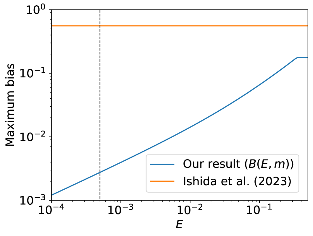
Figure 2: A comparison of our bias bound (Corollary˜2) and the existing bound by Ishida et al. (2023) with $n=10000,\ m=50$. The dashed line indicates the test error ($0.05$%) of the SOTA model for the binarized CIFAR-10 dataset, which we can use as $E$ in Corollary˜2. Our bound is over 200 times tighter than the existing one in this setup.

The function $B(E,m)$ can be computed numerically without any information about the data distribution, except for an upper bound of the Bayes error, $E$. Figure˜2 shows the magnitude of our lower bound, $B(E,m)$, for various values of $E$ (the blue line). It also shows the existing bias bound by Ishida et al. (2023) (the orange line). This comparison demonstrates that Corollary˜2 is a substantial improvement over the existing result across the entire range of the parameter $E$.

Let us take the binarized CIFAR-10 test set as an example. It consists of $n=10000$ instances, each of which has a soft label obtained as the average of around $m=50$ hard labels from the CIFAR-10H dataset. As the parameter $E$, we can use the Vision Transformer (Dosovitskiy et al., 2021)’s empirical error rate of $0.0005$ reported by Ishida et al. (2023), which is shown by the black dashed line in Figure˜2. While the existing bound suggests the bias of the hard-label-based estimator $\widehat{\mathrm{Err}^{*}}(\widehat{\eta}_{1:n})$ could be as large as $0.557$, our bound reveals the estimator is not that bad; indeed, it implies the bias is never larger than $0.00276$. In this case, our result is over $200$ times tighter than theirs.

Statistical consistency Theorem˜1 also implies the estimator $\widehat{\mathrm{Err}^{*}}(\widehat{\eta}_{1:n})$ is statistically consistent.

Corollary 3.

1. For any $\delta\in(0,1)$, with probability at least $1-\delta$, we have

   $$\left\lvert{\widehat{\mathrm{Err}^{*}}(\widehat{\eta}_{1:n})-\mathrm{Err}^{*}}\right\rvert\leq\sqrt{\frac{\log(2/\delta)}{2n}}+\sqrt{\frac{\pi}{2m}}\text{.}$$ (7)

2. Suppose there exists a constant $c>0$ such that $\left\lvert{\eta(x)-0.5}\right\rvert\geq c$ holds almost surely. Then, for any $\delta\in(0,1)$, with probability at least $1-\delta$, we have

   $$\left\lvert{\widehat{\mathrm{Err}^{*}}(\widehat{\eta}_{1:n})-\mathrm{Err}^{*}}\right\rvert\leq\sqrt{\frac{\log(2/\delta)}{2n}}+\frac{1-4c^{2}}{8cm}\text{.}$$ (8)

3 Estimation from currupted soft labels

This section tackles a more challenging setting where we do not have access to the true posterior probability $\eta$. This setting reflects many real-world problems, such as in medical diagnosis where a doctor’s subjective confidence in their decision can be regarded as a soft label, or when practitioners provide automated soft labels with LLMs in place of human annotators. However, there is no guarantee that it exactly reflects the true underlying probability.

In this section, we consider a problem setting where each instance $x_{i}$ is given a real number $\tilde{\eta}_{i}\in[0,1]$, which is expected to approximate the clean soft label $\eta_{i}$ in some sense but not necessarily identical to $\eta_{i}$. We call $\left\{{\tilde{\eta}_{i}}\right\}_{i=1}^{n}$ corrupted soft labels. How can we estimate the Bayes error when only corrupted soft labels are available instead of clean ones? Estimation with a provable guarantee will be impossible without some assumption on the quality of the soft labels. Then, what guarantee can be provided under what assumption?

3.1 Preliminaries

In addition to the preliminaries introduced in Section˜2.1, we briefly review a few more required for the discussion in this section.

Calibration  Predicting accurate class labels is not always sufficient in classification problems. It is often crucial to obtain reliable probability estimates, especially in high-stakes applications including personalized medicine (Jiang et al., 2012) and meteorological forecasting (Murphy, 1973; DeGroot and Fienberg, 1983).

A popular notion to capture the quality of probability estimates is calibration. A probabilistic classifier $c$ is said to be well-calibrated if the predicted probabilities closely match the actual frequencies of the class labels (Kull et al., 2017), i.e., $c(x)=\operatorname*{\mathbb{E}}\left[{y\mid c(x)}\right]$ almost surely. While one might hope that a perfectly calibrated output $c(x)$ matches the posterior probability $\operatorname*{\mathbb{E}}\left[{y\mid x}\right]=\mathbb{P}(y=1\mid x)$, it is not necessarily true. Indeed, calibration is a weaker notion and just a necessary condition for $c(x)=\operatorname*{\mathbb{E}}\left[{y\mid x}\right]$. For example, even a constant predictor $c(x)\equiv\operatorname*{\mathbb{P}}\left({y=1}\right)$ is well-calibrated although it can be far from $\operatorname*{\mathbb{P}}\left({y=1\mid x}\right)$.

It is known that many machine learning models, including modern neural networks, are not calibrated out of the box (Zadrozny and Elkan, 2001; Guo et al., 2017). Therefore, their outputs have to be recalibrated in post-processing, and various methods have been proposed to achieve this goal. They can be roughly categorized into two groups, namely parametric and nonparametric methods. The former includes Platt scaling (Platt, 1999), also known as logistic calibration (Kull et al., 2017), and beta calibration (Kull et al., 2017). Among the latter category are histogram binning (Zadrozny and Elkan, 2001) and isotonic calibration (Zadrozny and Elkan, 2002). Each of these methods requires a dataset $\left\{{(c_{i},y_{i})}\right\}_{i=1}^{n}$ to obtain a function that takes the output of an uncalibrated predictor $c$ and transforms it into a reliable probability estimate. This function is sometimes called a calibration map (Kull et al., 2017, 2019). Here, $c_{i}=c(x_{i})$ is the output of $c$ for an instance $x_{i}$, and $y_{i}$ is the corresponding class label. To avoid overfitting, each $(x_{i},y_{i})$ needs to be sampled independently of the training set used to obtain the predictor $c$.

Isotonic calibration Here, we briefly describe the algorithm of isotonic calibration (Zadrozny and Elkan, 2002), arguably one of the most commonly used nonparametric recalibration methods, as it plays an important role in this paper. Suppose a dataset $\left\{{(c_{i},y_{i})}\right\}_{i=1}^{n}$ is given. The algorithm proceeds as follows. First, the dataset $(c_{1},y_{1}),\dots,(c_{n},y_{n})$ is reordered into $\left({c_{(1)},y_{(1)}}\right),\dots,\left({c_{(n)},y_{(n)}}\right)$ so that the resulting sequence $c_{(1)},\dots,c_{(n)}$ of outputs becomes non-decreasing. Then, we find a non-decreasing sequence $0\leq c^{\prime}_{(1)}\leq\dots\leq c^{\prime}_{(n)}\leq 1$ such that it minimizes the squared error $\frac{1}{n}\sum_{i=1}^{n}\left({y_{(i)}-c^{\prime}_{(i)}}\right)^{2}$. Finally, for each $i\in[n]$, $c^{\prime}_{(i)}$ is assigned as the calibrated version of $c_{(i)}$. This procedure is a special case of isotonic regression, one of the most well-studied shape-constrained regression problems.

3.2 Proposed method

We propose a simple approach where we first calibrate the corrupted soft labels and then plug them into the formula (1) for clean soft labels. Although calibration was originally developed for transforming the output scores of classifiers into reliable probability estimates, here we suggest using it for corrupted soft labels. We assume that, for each $i\in[n]$, we are given a corrupted soft label $\tilde{\eta}_{i}\in[0,1]$ and a single hard label $y_{i}\in\left\{{0,1}\right\}$ sampled from the true posterior distribution $\mathbb{P}(y\mid x=x_{i})$. We use the hard labels $\left\{{y_{i}}\right\}_{i=1}^{n}$ to calibrate the soft labels $\left\{{\tilde{\eta}_{i}}\right\}_{i=1}^{n}$ using some calibration algorithm $\mathcal{A}$. We write $\widehat{\eta}_{i}^{\mathcal{A}}$ to represent the resulting calibrated soft labels. Finally, we estimate the Bayes error $\mathrm{Err}^{*}$ by $\widehat{\mathrm{Err}^{*}}\left({\widehat{\eta}_{1:n}^{\mathcal{A}}}\right)=\frac{1}{n}\sum_{i=1}^{n}\min\left\{{\widehat{\eta}_{i}^{\mathcal{A}},1-\widehat{\eta}_{i}^{\mathcal{A}}}\right\}$.

However, as we mentioned earlier, even perfect calibration does not necessarily imply that the resulting soft labels are accurate estimates of the clean soft labels. A simple example illustrates this limitation:

Example 2.

Consider drawing instances from a mixture of two distributions over $\mathcal{X}$ with disjoint supports, and let us set the mixture rate $\theta$ to be $0.5$. The true Bayes error is trivially $0$. If $\mathcal{A}$ is a calibration algorithm that produces constant soft labels $\widehat{\eta}_{i}^{\mathcal{A}}=\theta=0.5$ for all $i\in[n]$, it indeed achieves perfect calibration. However, the resulting estimate of the Bayes error is $\min\left\{{\theta,1-\theta}\right\}=0.5$, which deviates significantly from the true value $0$.

Therefore, estimation with a provable guarantee will not be possible for arbitrary calibration algorithms or without any assumptions on the soft labels. What calibration algorithm can achieve reliable estimation under what assumption? In Section˜3.3, we provide the first answer to this question.

3.3 Theoretical guarantee for isotonic calibration

Here, we propose choosing isotonic calibration (Zadrozny and Elkan, 2002) as the calibration algorithm $\mathcal{A}$ and indentify a condition under which we can consistently estimate the Bayes error with our method. Specifically, we estimate the Bayes error by the following procedure:

1. Reorder $(\tilde{\eta}_{1},y_{1}),\dots,(\tilde{\eta}_{n},y_{n})$ into $\left({\tilde{\eta}_{(1)},y_{(1)}}\right),\dots,\left({\tilde{\eta}_{(n)},y_{(n)}}\right)$ so that the resulting sequence $\tilde{\eta}_{(1)},\dots,\tilde{\eta}_{(n)}$ of outputs becomes non-decreasing.

2. Find a non-decreasing sequence $0\leq\widehat{\eta}^{\mathrm{iso}}_{(1)}\leq\dots\leq\widehat{\eta}^{\mathrm{iso}}_{(n)}\leq 1$ such that it minimizes the squared error $\frac{1}{n}\sum_{i=1}^{n}\left({y_{(i)}-\widehat{\eta}^{\mathrm{iso}}_{(i)}}\right)^{2}$. This gives us isotonic-calibrated soft labels $\widehat{\eta}_{(1)}^{\mathrm{iso}},\dots,\widehat{\eta}_{(n)}^{\mathrm{iso}}$.

3. Estimate the Bayes error as $\widehat{\mathrm{Err}^{*}}(\widehat{\eta}_{1:n}^{\mathrm{iso}})=\frac{1}{n}\sum_{i=1}^{n}\min\left\{{\widehat{\eta}_{(i)}^{\mathrm{iso}},1-\widehat{\eta}_{(i)}^{\mathrm{iso}}}\right\}$.

The next theorem is the main theoretical result of this section, which states that we can construct a consistent estimator of the Bayes error using isotonic calibration as long as the soft labels’ order is preserved. See Appendix˜C for the proof.

Theorem 2.

Suppose that there exists an increasing function $f$ such that $\tilde{\eta}_{i}=f(\eta_{i})$ almost surely. Then, for any $\delta\in(0,1)$, with probability at least $1-\delta$, we have

$$\left\lvert{\widehat{\mathrm{Err}^{*}}(\widehat{\eta}_{1:n}^{\mathrm{iso}})-\mathrm{Err}^{*}}\right\rvert\leq\frac{C}{n^{1/3}}+2\sqrt{\frac{2\log(2/\delta)}{n}}\text{,}$$ (9)

where $C>0$ is a constant.

Note that the assumption of Theorem˜2 is a relaxation of the availability of clean soft labels since we can take the identity map as $f$ when $\tilde{\eta}_{i}=\eta_{i}$. In other words, the original work by Ishida et al. (2023) assumes that we have access to the exact values of the clean soft labels, whereas our proposed method only requires the knowledge of their order.

4 Experiments

In this section, we perform an experiment where we estimate the Bayes error of synthetic and real-world datasets using our proposed method.

4.1 Experimental settings

The methods employed in this experiment are the following: 1. clean: the estimator with clean soft labels, i.e., $\widehat{\mathrm{Err}^{*}}\left({\eta_{1:n}}\right)$, 2. hard: the estimator with approximate soft labels obtained as averaged hard labels, i.e., $\widehat{\mathrm{Err}^{*}}\left({\widehat{\eta}_{1:n}}\right)$, 3. corrupted: the estimator with corrupted soft labels, i.e., $\widehat{\mathrm{Err}^{*}}\left({\tilde{\eta}_{1:n}}\right)$, and 4. The estimator with soft labels obtained by calibrating the corrupted soft labels, i.e., $\widehat{\mathrm{Err}^{*}}\left({\widehat{\eta}_{1:n}^{\mathcal{A}}}\right)$. We use the following as the calibration algorithm $\mathcal{A}$: isotonic calibration (isotonic; Zadrozny and Elkan (2002)), uniform-mass histogram binning (Zadrozny and Elkan, 2001) with $10,25,50$ and $100$ bins (hist-10, hist-25, hist-50 and hist-100), and beta calibration (beta; Kull et al. (2017)). We use $1000$ bootstrap resamples to compute a 95% confidence interval for each method.

Datasets We conduct our experiments using several datasets. The first one is a two-dimensional synthetic dataset of size $n=10000$ generated from a Gaussian mixture $\mathbb{P}_{\mathcal{X}}=0.6\cdot\mathbb{P}_{0}+0.4\cdot\mathbb{P}_{1}$, where $\mathbb{P}_{0}=N\left({(0,0),I_{2}}\right)$, $\mathbb{P}_{1}=N\left({(2,2),I_{2}}\right)$ and $I_{d}$ is the $d$-by-$d$ identity matrix. We use $m=50$ hard labels per instance in the hard setup. For each $i\in[n]$, we generated the corrupted version $\tilde{\eta}_{i}$ of the soft label $\eta_{i}$ by $\tilde{\eta}_{i}=f(\eta_{i};2,0.7)$, where $f(p;a,b)=\left({1+\left({\frac{1-p}{p}}\right)^{1/a}\frac{1-b}{b}}\right)^{-1},\ 0<p<1,\ a\geq 0,\ 0<b<1$. The function $f$ is the inverse function of the two-parameter beta calibration map (Kull et al., 2017) and can express various continuous increasing transformations on the interval $(0,1)$ depending on the parameters $a$ and $b$. Figure˜3 shows the graph of the corruption function $f$. As can be seen in the figure, it pushes probability values away from zero or one, making the soft labels ‘‘unconfident.’’ It also distorts soft labels so that $\eta_{i}=0.5$ is mapped to $\tilde{\eta}_{i}=f(\eta_{i})=b$. Note that $f$ satisfies the assumption of Theorem˜2 since it is increasing. We also explored other sets of parameters and other types of corruption; see Appendix˜D for details.

Figure 3: The corruption function $f(p;a,b)$ with parameters $a=2,\ b=0.7$.

The second dataset is the test set of CIFAR-10 (Krizhevsky, 2009) with soft labels taken from the CIFAR-10H dataset (Peterson et al., 2019). Since they are originally multi-class datasets, we reconstruct a binary dataset by relabeling the animal-related classes (bird, cat, deer, dog, frog and horse) as positive and the rest as negative, similarly to what Ishida et al. (2023) did in their experiments. We cannot experiment with the clean setup as clean soft labels are unavailable for real-world datasets. Therefore, we conduct our experiment only for corrupted/isotonic/hist/beta using soft labels from CIFAR-10H as corrupted ones. Recall that the CIFAR-10H soft labels can be considered to be corrupted because of the mismatched labeling distributions, as we mentioned in Section˜1. We compare the estimated Bayes error with the test error of a Vision Transformer (ViT) (Dosovitskiy et al., 2021) on this dataset reported by Ishida et al. (2017), which is 0.05%.

We also experimented with the Fashion-MNIST dataset (Xiao et al., 2017) and its soft-labeled counterpart, Fashion-MNIST-H (Ishida et al., 2023). Following Ishida et al. (2023), we binarized the dataset by treating T-shirt/top, pullover, dress, coat and shirt as the positive class. The rest proceeds similarly to the CIFAR-10 experiment except that we newly trained a ResNet-18 (He et al., 2016) in place of the ViT. Details such as training parameters can be found in Appendix˜D.

(a) Synthetic dataset

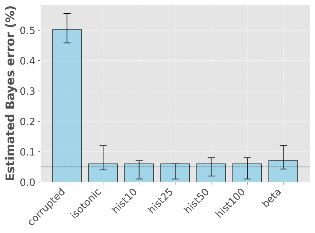
(b) CIFAR-10

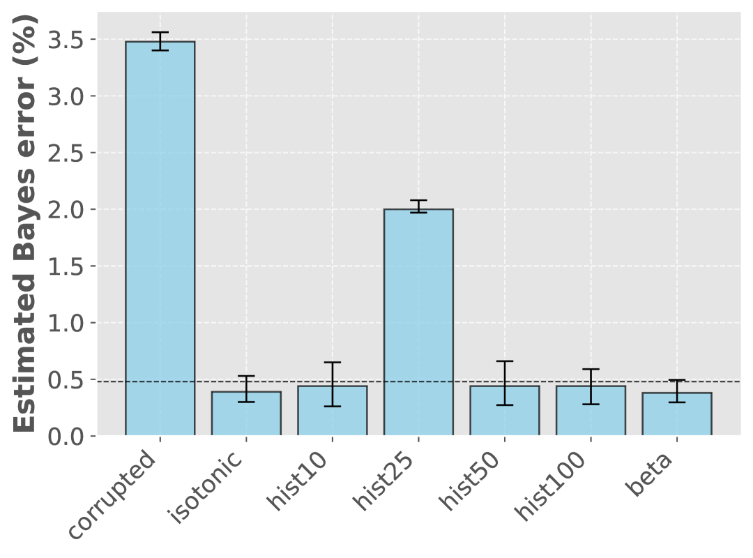
(c) Fashion-MNIST

Figure 4: The estimated Bayes error for the synthetic dataset, CIFAR-10, and Fashion-MNIST, obtained with various methods. Error bars denote 95% bootstrap confidence intervals. For CIFAR-10, the ViT test error is indicated by a horizontal dashed line, while for Fashion-MNIST the dashed line marks the ResNet-18 test error.

4.2 Results

Figure˜4 shows the result of the experiments. The black dashed lines in Figure˜4(b) and Figure˜4(c) indicate the test error of a classifier trained for each dataset. As expected, the unconfidence of the corrupted soft labels results in a severe overestimation of the Bayes error. All the calibration methods (isotonic/hist-*/beta) produce far more reasonable estimates compared with the baseline corrupted. For Fashion-MNIST, however, histogram binning sometimes fails to offer rational estimates, as you can see in Figure˜4(c). Specifically, hist-25 results in a Bayes error estimate substantially larger than the ResNet’s test error. This might be highlighting the necessity for a carefully chosen calibration method, as we mentioned in Section˜3.2. On the other hand, isotonic and beta consistently produce reasonable estimates.

4.3 Discussion

Although our calibration-based methods successfully mitigate over- or underestimation of the Bayes error, it is difficult to truly assess the validity of the estimates for real-world datasets since we do not have access to the underlying distributions. This is a fundamental challenge common across the field of Bayes error estimation. Early attempts to solve it have appeared in recent years, e.g., Renggli et al. (2021), and we see advancing these approaches as an important direction for future work. Another limitation is that the theoretical guarantee in Theorem˜2 relies on the assumption that corruption does not change the order of soft labels, which might not always be satisfied in practice. We have not yet reached a theoretical understanding of how much violating this assumption hurts the estimation accuracy. However, we do attempt to investigate this problem empirically; see Section˜D.3 for details.

5 Conclusion

In this paper, we discussed the estimation of the Bayes error in binary classification. In Section˜2, we significantly improved the existing bound on the bias of the hard-label-based estimator. We also revealed that the decay rate of the bias depends on how well the two class-conditional distributions are separated, and it can decay in a much faster rate than the previous result suggested. In Section˜3, we tackled a challenging problem of Bayes error estimation from corrupted soft labels and proposed an estimator based on calibration. After presenting an example highlighting the importance of choosing appropriate calibration algorithms, we proved that we can construct a statistically consistent estimator using isotonic calibration as long as the original soft labels are correctly ordered. Then, our theory was validated by numerical experiments with synthetic and real-world datasets in Section˜4.

Finally, we discuss possible future directions. As we mentioned in Section˜4.3, it is still unclear from Theorem˜2 how much the estimation accuracy of the calibration-based estimator is degraded when the assumption that the order of soft labels are preserved. Seeking for such understandings is our important future work. Another possible direction is the extension to multi-class problems. Investigating theoretical guarantees for calibration algorithms other than isotonic calibration is also an interesting direction.

Appendix A Related work

Estimation of the Bayes error $\mathrm{Err}^{*}$ (see Section 2.1 for the definition) is a classical problem in the field of machine learning and pattern recognition. Existing methods for Bayes error estimation can be categorized based on the type of data used, specifically as either instance-label pair-based or soft label-based estimation.

Most of the existing methods require a dataset $\left\{{(x_{i},y_{i})}\right\}_{i=1}^{n}$ composed of instances $x_{i}\in\mathcal{X}$ paired with their respective labels $y_{i}\in\mathcal{Y}=\left\{{0,1}\right\}$. Assuming the two class-conditional distributions of instances have densities satisfying certain conditions, Berisha et al. (2014), Moon et al. (2018) and Noshad et al. (2019) proposed approaches based on the estimation of $f$-divergence between the class-conditional densities. Specifically, Berisha et al. (2014) and Moon et al. (2018) suggested estimating upper or lower bounds and thus their methods suffer from relatively large biases. Although Noshad et al. (2019) succeeded in estimating the exact Bayes error instead of bounds on it, they assumed that the class-conditional densities $p_{0},p_{1}$ are Hölder-continuous and satisfy $0<L\leq p_{i}\leq U\ (i=0,1)$ for some constants $L$ and $U$, and their estimator requires the knowledge of the values of these constants, which can be unpractical.

On the other hand, Theisen et al. (2021) proposed a Bayes error estimation method based on normalizing flow models (Papamakarios et al., 2021; Kingma and Dhariwal, 2018). They first showed that the Bayes error is invariant under invertible transformations. Using this result, they suggested approximating the data distribution with a normalizing flow and then computing the Bayes error for its base Gaussian distribution, which can be done using the Holmes--Diaconis--Ross integration scheme (Diaconis and Holmes, 1995; Gessner et al., 2020). One of the drawbacks of their approach is that it is prohibitively memory-intensive for high-dimensional data, as mentioned in their paper.

The method proposed by Ishida et al. (2023), described in Section˜2.1, was unique in that it utilized the soft labels $\eta_{i}=\eta(x_{i})$ instead of the instances $x_{i}$ themselves. Jeong et al. (2023) extended the approach of Ishida et al. (2023) to the estimation of the Bayes error in multi-class classification problems.

Appendix B Supplementary for Section 2

B.1 Proof of Theorem˜1

For each $i=1,\ldots,d$, let $\widehat{p}_{i}=\frac{1}{m}\sum_{j=1}^{m}Z_{i}^{(j)}$ where $Z_{i}^{(1)},\ldots,Z_{i}^{(m)}\in\left\{{0,1}\right\}$ are independent Bernoulli random variables with mean $p_{i}$. For ease of notation, we denote $\widehat{p}=(\widehat{p}_{1},\ldots,\widehat{p}_{d})$ and $p=(p_{1},\ldots,p_{d})$. Noting that $\operatorname*{\mathbb{E}}\left[{\widehat{p}}\right]=p$, $\widehat{p}$ is an unbiased and consistent estimator of $p$.

Suppose that we would like to estimate the value $\phi(p)$ for some function $\phi:\mathbb{R}^{d}\to\mathbb{R}$. It is natural to consider a plug-in estimator $\phi(\widehat{p})$. We can evaluate its bias $\operatorname*{\mathbb{E}}\left[{\phi(\widehat{p})}\right]-\phi(p)=\operatorname*{\mathbb{E}}\left[{\phi(\widehat{p})}\right]-\phi\left({\operatorname*{\mathbb{E}}\left[{\widehat{p}}\right]}\right)$ using Theorem˜3, which is a sharpened version of Jensen’s inequality that we newly tailored by extending the result by Liao and Berg (2019). We spare a separate subsection for its proof and further discussions as it might be of independent interest; see Section˜B.3 for more details.

Lemma 1.

Suppose $\phi$ is differentiable at $\mu$. Then, for any $a\in\mathbb{R}^{d}$, we have

$$\frac{\inf_{z}h(z;a)}{m}\sum_{i=1}^{d}p_{i}(1-p_{i})\leq\operatorname*{\mathbb{E}}\left[{\phi(\widehat{p})}\right]-\phi(p)\leq\frac{\sup_{z}h(z;a)}{m}\sum_{i=1}^{d}p_{i}(1-p_{i})\text{,}$$ (10)

where $h$ is defined in (52).

Proof.

For any $i,j\in[d]$, we have

$$\operatorname*{\mathbb{E}}\left[{(\widehat{p}_{i}-p_{i})(\widehat{p}_{j}-p_{j})}\right]=\frac{1}{m}p_{i}(1-p_{i})\delta_{ij}\text{,}$$ (11)

where $\delta_{ij}=\mathbbm{1}\left[{i=j}\right]$ is the Kronecker delta. This implies

$$\operatorname{tr}\left({\operatorname*{\mathrm{Cov}}\left[{\,\widehat{p}\,}\right]}\right)=\frac{1}{m}\sum_{i=1}^{d}p_{i}(1-p_{i})\text{.}$$ (12)

Plugging this into our generalized Jensen inequality (Theorem˜3) concludes the proof. ∎

It is often the case that the function $\phi$ in question is Lipschitz continuous. For example, every convex function is locally Lipschitz on any convex compact subset of the relative interior of its domain (see e.g. Hiriart-Urruty and Lemaréchal, 1993, Theorem 3.1.2 in Chapter IV). In such cases, we can derive another type of bound based on Lipschitzness.

Lemma 2 (Lipschitzness-based bounds for the bias).

If $\phi$ is $L$-Lipschitz with respect to the $1$-norm, we have

$$\left\lvert{\operatorname*{\mathbb{E}}\left[{\phi(\widehat{p})}\right]-\phi(p)}\right\rvert\leq Ld\sqrt{\frac{\pi}{2m}}\text{.}$$ (13)

Proof.

First of all, it holds that

$$\left\lvert{\operatorname*{\mathbb{E}}\left[{\phi(\widehat{p})}\right]-\phi(p)}\right\rvert\leq \operatorname*{\mathbb{E}}\left[{\left\lvert{\phi(\widehat{p})-\phi(p)}\right\rvert}\right]$$ (14)

$$\leq L\operatorname*{\mathbb{E}}\left[{\sum_{i=1}^{d}\left\lvert{\widehat{p}_{i}-p_{i}}\right\rvert}\right]\quad\text{(by Lipschitzness)}$$ (15)

$$= L\sum_{i=1}^{d}\operatorname*{\mathbb{E}}\left[{\left\lvert{\widehat{p}_{i}-p_{i}}\right\rvert}\right]\text{.}$$ (16)

Each summand can be bounded by integrating Hoeffding’s tail bound (see, e.g., Theorem 2.2.6 of (Vershynin, 2018)):

$$\operatorname*{\mathbb{E}}\left[{\left\lvert{\widehat{p}_{i}-p_{i}}\right\rvert}\right] =\int_{0}^{\infty}\operatorname*{\mathbb{P}}\left({\left\lvert{\widehat{p}_{i}-p_{i}}\right\rvert\geq t}\right)\,dt$$ (17)

$$\leq\int_{0}^{\infty}2\exp(-2mt^{2})\,dt$$ (18)

$$=\sqrt{\frac{\pi}{2m}}\text{.}$$ (19)

Hence the result follows. ∎

Lemma˜2 suggests that the bias is at most $\mathcal{O}(1/\sqrt{m})$, whereas Lemma˜1 indicates a faster convergence rate of $\mathcal{O}(1/m)$ whenever the supremum and infimum are finite.

Now, define

$$\phi_{\mathrm{Err}}(z)\coloneqq\min\left\{{z,1-z}\right\}$$ (20)

for $z\in[0,1]$. We choose $\phi=\phi_{\mathrm{Err}}$ and apply Lemma˜1 and Lemma˜2 to show the following lemma.

Lemma 3.

For each $i\in[d]$, we have

$$-\sqrt{\frac{\pi}{2m}}\leq\operatorname*{\mathbb{E}}\left[{\phi_{\mathrm{Err}}(\widehat{p}_{i})}\right]-\phi_{\mathrm{Err}}(p_{i})\leq 0\text{.}$$ (21)

Furthermore, if $p_{i}\neq 0.5$, it holds that

$$-\frac{p_{i}(1-p_{i})}{m\lvert 2p_{i}-1\rvert}\leq\operatorname*{\mathbb{E}}\left[{\phi_{\mathrm{Err}}(\widehat{p}_{i})}\right]-\phi_{\mathrm{Err}}(p_{i})\leq 0\text{.}$$ (22)

Proof.

The lower bound of the first inequality is a direct consequences of Lemma˜2 and the fact that $\phi_{\mathrm{Err}}$ is $1$-Lipschitz. The upper bound follows from the concavity of $\phi_{\mathrm{Err}}$ and the classic Jensen inequality.

To prove the second inequality, we first assume $0\leq p_{i}<0.5$. For any $z\in[0,1]\setminus\left\{{p_{i}}\right\}$, we have

$$h\left({z;1}\right)=\frac{\phi_{\mathrm{Err}}(z)-\phi_{\mathrm{Err}}(p_{i})-\left({z-p_{i}}\right)}{(z-p_{i})^{2}}=\begin{dcases*}0&for $z\in[0,0.5]$,\\ \frac{1-2z}{(z-p_{i})^{2}}&for $z\in[0.5,1]$.\end{dcases*}$$ (23)

Taking $h(p_{i};1)\coloneqq 0$, some calculation reveals that

$$-\frac{1}{1-2p_{i}}\leq h(z;1)\leq 0\text{,}\quad\forall\,z\in[0,1]\text{.}$$ (24)

Therefore, Lemma˜1 implies

$$-\frac{p_{i}(1-p_{i})}{m(1-2p_{i})}\leq\operatorname*{\mathbb{E}}\left[{\phi_{\mathrm{Err}}(\widehat{p}_{i})}\right]-\phi_{\mathrm{Err}}(p_{i})\leq 0\text{.}$$ (25)

Next, we assume $0.5<p_{i}\leq 1$. A similar argument proves $-\frac{1}{2p_{i}-1}\leq h(z;-1)\leq 0$ and

$$-\frac{p_{i}(1-p_{i})}{m(2p_{i}-1)}\leq\operatorname*{\mathbb{E}}\left[{\phi_{\mathrm{Err}}(\widehat{p}_{i})}\right]-\phi_{\mathrm{Err}}(p_{i})\leq 0\text{.}$$ (26)

Combining (25) and (26) proves the second bound. ∎

Note that Lemma˜3 can be rewritten as

$$-\min\left\{{\frac{L_{\mathrm{Err}}(p_{i})}{m},\ \sqrt{\frac{\pi}{2m}}}\right\}\leq\operatorname*{\mathbb{E}}\left[{\phi_{\mathrm{Err}}(\widehat{p}_{i})}\right]-\phi_{\mathrm{Err}}(p_{i})\leq 0\text{,}$$ (27)

where

$$L_{\mathrm{Err}}(q)=\begin{dcases*}\frac{q(1-q)}{\left\lvert{2q-1}\right\rvert}&if $q\neq 0.5$,\\ +\infty&if $q=0.5$.\end{dcases*}$$ (28)

Figure˜5 shows the graph of the function $L_{\mathrm{Err}}$. Finally, Theorem˜1 is proved as follows.

Proof of Theorem˜1.

Conditioning on $x$, let $\left\{{y^{(j)}}\right\}_{j=1}^{m}$ be independent Bernoulli random variables with mean $\eta(x)$ and $\widehat{\eta}$ be their average $\frac{1}{m}\sum_{j=1}^{m}y^{(j)}$. Then, Lemma˜3 gives

$$-\min\left\{{\frac{L_{\mathrm{Err}}(\eta(x))}{m},\ \sqrt{\frac{\pi}{2m}}}\right\}\leq\operatorname*{\mathbb{E}}\left[{\phi_{\mathrm{Err}}(\widehat{\eta})\mid x}\right]-\phi_{\mathrm{Err}}(\eta(x))\leq 0\text{.}$$ (29)

By taking expectation over $x$, we obtain

$$-\operatorname*{\mathbb{E}}\left[{\min\left\{{\frac{L_{\mathrm{Err}}(\eta(x))}{m},\ \sqrt{\frac{\pi}{2m}}}\right\}}\right]\leq\operatorname*{\mathbb{E}}\left[{\phi_{\mathrm{Err}}(\widehat{\eta})}\right]-\operatorname*{\mathbb{E}}\left[{\phi_{\mathrm{Err}}(\eta(x))}\right]\leq 0\text{.}$$ (30)

Now the claim follows since $\operatorname*{\mathbb{E}}\left[{\widehat{\mathrm{Err}^{*}}(\widehat{\eta}_{1:n})}\right]=\operatorname*{\mathbb{E}}\left[{\phi_{\mathrm{Err}}(\widehat{\eta})}\right]$ and $\mathrm{Err}^{*}=\operatorname*{\mathbb{E}}\left[{\phi_{\mathrm{Err}}(\eta(x))}\right]$. ∎

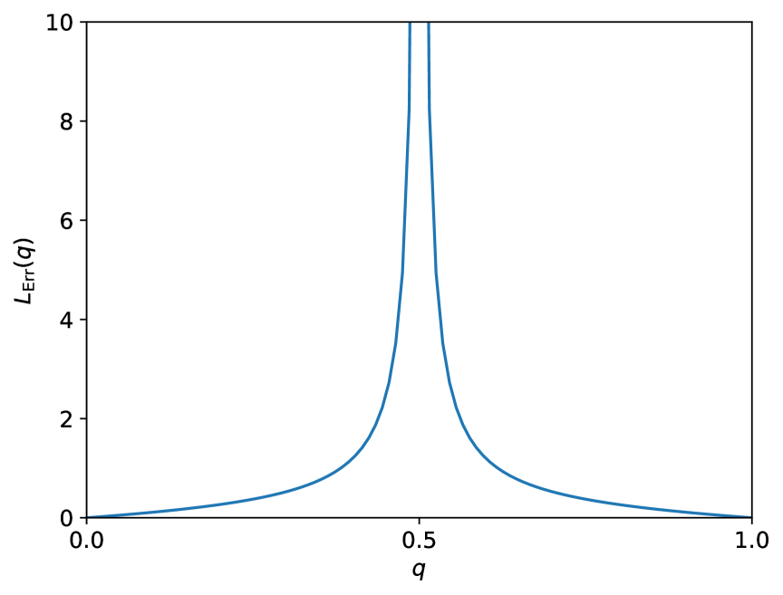
Figure 5: The graph of the function $L_{\mathrm{Err}}$.

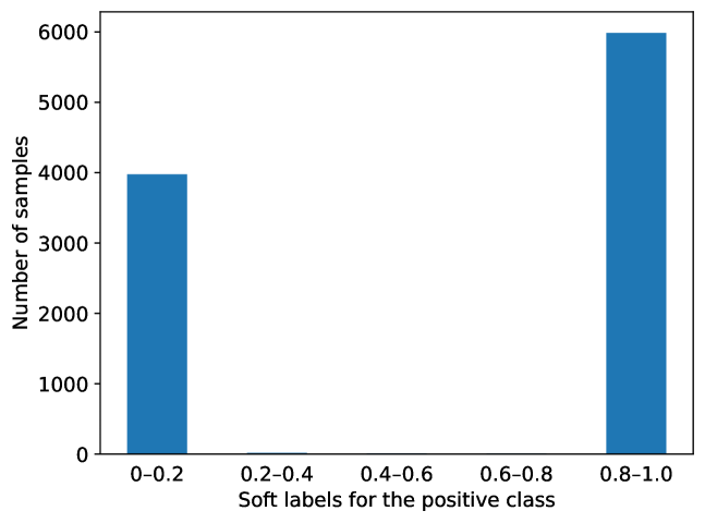
Figure 6: The distribution of the soft labels for the positive class in the binarized CIFAR-10H dataset (see Section˜4.1 for details). You can see the two classes are very well-separated.

B.2 Proofs for other results

B.2.1 Superiority of Theorem˜1 over the existing result

Proposition 1.

Theorem˜1 is tighter than the existing result (2) by Ishida et al. (2023) for all $n,m\geq 1$.

Proof.

Our upper bound $0$ is of course smaller than the upper bound in (2). As for the lower bounds, we can see that the condition

$$\sqrt{\frac{\pi}{2m}}\leq\frac{1}{2\sqrt{m}}+\sqrt{\frac{\log(2n\sqrt{m})}{m}}$$ (31)

is equivalent to

$$n\sqrt{m}\geq\frac{1}{2}\exp\left({\left({\frac{\sqrt{2\pi}-1}{2}}\right)^{2}}\right)\text{.}$$ (32)

The right-hand side is less than $1$ so (32) always holds. ∎

B.2.2 Faster decay rate of the bias in well-separated cases (Corollary˜1 & Example˜1)

Proof of Corollary˜1.

By the assumption, we have

$$L_{\mathrm{Err}}(\eta(x))=\frac{\eta(x)(1-\eta(x))}{2\left\lvert{\eta(x)-0.5}\right\rvert}\leq\frac{1/4-c^{2}}{2c}$$ (33)

almost surely. Combining this with Theorem˜1, we obtain the result. ∎

Proof of Example˜1.

Let $f_{0},f_{1}$ be the densities of $\mathcal{F}_{0},\mathcal{F}_{1}$, respectively. From the data generation model, we can see that

$$\eta(x)=\frac{\nu f_{0}(x)+(1-\nu)f_{1}(x)}{f_{0}(x)+f_{1}(x)}$$ (34)

for any $x\in\mathcal{X}$ such that $f_{0}(x)>0$ or $f_{1}(x)>0$. Since the supports of $\mathcal{F}_{0},\mathcal{F}_{1}$ are disjoint, we can assume that

$$f_{0}(x)>0\implies f_{1}(x)=0,\quad f_{1}(x)>0\implies f_{0}(x)=0\quad\text{for any $x\in\mathcal{X}$,}$$ (35)

which implies

$$\eta(x)=\begin{dcases*}\nu&\text{if $f_{0}(x)>0$,}\\ 1-\nu&\text{if $f_{1}(x)>0$.}\end{dcases*}$$ (36)

Therefore, it holds that

$$\left\lvert{\eta(x)-0.5}\right\rvert=\left\lvert{\nu-0.5}\right\rvert=c>0$$ (37)

almost surely. ∎

B.2.3 Computable bound of the bias (Corollary˜2)

Lemma 4.

If $\mathrm{Err}^{*}\leq E$, we have

$$\operatorname*{\mathbb{P}}\left({\phi_{\mathrm{Err}}(\eta(x))\geq t}\right)\leq\min\left\{{1,\frac{E}{t}}\right\}$$ (38)

for any $t\in(0,1/2]$.

Proof.

Since $\phi_{\mathrm{Err}}(\eta(x))$ is a non-negative random variable with mean $\operatorname*{\mathbb{E}}\left[{\phi_{\mathrm{Err}}(\eta(x))}\right]=\mathrm{Err}^{*}$, Markov’s inequality gives

$$\operatorname*{\mathbb{P}}\left({\phi_{\mathrm{Err}}(\eta(x))\geq t}\right)\leq\frac{\mathrm{Err}^{*}}{t}\leq\frac{E}{t}$$ (39)

for any $t>0$. ∎

Proof of Corollary˜2.

Let $z=\phi_{\mathrm{Err}}(\eta(x))$. Since

$$\frac{\eta(x)(1-\eta(x))}{\left\lvert{2\eta(x)-1}\right\rvert}=\frac{z(1-z)}{1-2z}\text{,}$$ (40)

we have

$$\frac{\eta(x)(1-\eta(x))}{\left\lvert{2\eta(x)-1}\right\rvert}<\frac{t(1-t)}{1-2t}$$ (41)

if $z<t$. Therefore,

$$\operatorname*{\mathbb{E}}\left[{\min\left\{{\frac{L_{\mathrm{Err}}(\eta(x))}{m},\ \sqrt{\frac{\pi}{2m}}}\right\}}\right]$$ (42)

$$\leq\operatorname*{\mathbb{E}}\left[{\sqrt{\frac{\pi}{2m}}\cdot\mathbbm{1}\left[{z\geq t}\right]+\frac{1}{m}\cdot\frac{t(1-t)}{1-2t}\cdot\mathbbm{1}\left[{z<t}\right]}\right]$$ (43)

$$\leq\sqrt{\frac{\pi}{2m}}\cdot\operatorname*{\mathbb{P}}\left({z\geq t}\right)+\frac{1}{m}\cdot\frac{t(1-t)}{1-2t}\cdot 1\text{.}$$ (44)

By using Lemma˜4, we obtain

$$\operatorname*{\mathbb{E}}\left[{\min\left\{{\frac{L_{\mathrm{Err}}(\eta(x))}{m},\ \sqrt{\frac{\pi}{2m}}}\right\}}\right]\leq\sqrt{\frac{\pi}{2m}}\cdot\min\left\{{1,\frac{E}{t}}\right\}+\frac{1}{m}\cdot\frac{t(1-t)}{1-2t}\text{.}$$ (45)

Combining this with Theorem˜1 yields the result. ∎

B.2.4 Statistical consistency (Corollary˜3)

Proof of Corollary˜3.

By Hoeffding’s inequality, we have

$$\left\lvert{\widehat{\mathrm{Err}^{*}}(\widehat{\eta}_{1:n})-\operatorname*{\mathbb{E}}\left[{\widehat{\mathrm{Err}^{*}}(\widehat{\eta}_{1:n})}\right]}\right\rvert$$ (46)

$$\leq\left\lvert{\widehat{\mathrm{Err}^{*}}(\widehat{\eta}_{1:n})-\operatorname*{\mathbb{E}}\left[{\widehat{\mathrm{Err}^{*}}(\widehat{\eta}_{1:n})}\right]}\right\rvert+\left\lvert{\operatorname*{\mathbb{E}}\left[{\widehat{\mathrm{Err}^{*}}(\widehat{\eta}_{1:n})}\right]-\mathrm{Err}^{*}}\right\rvert$$ (47)

$$\leq\sqrt{\frac{\log(2/\delta)}{2n}}+\left\lvert{\operatorname*{\mathbb{E}}\left[{\widehat{\mathrm{Err}^{*}}(\widehat{\eta}_{1:n})}\right]-\mathrm{Err}^{*}}\right\rvert$$ (48)

with probability greater than $1-\delta$. By upper-bounding the second term using Theorem˜1 and Corollary˜1, we obtain (7) and (8), respectively. ∎

B.3 Generalized Jensen inequality

Here, we discuss our generalization of the Jensen inequality used in the proof of Theorem˜1 in detail.

The celebrated Jensen inequality states that we have

$$\operatorname*{\mathbb{E}}\left[{\phi(Z)}\right]\geq\phi(\operatorname*{\mathbb{E}}\left[{Z}\right])$$ (49)

for any convex function $\phi:A\subset\mathbb{R}^{d}\to\mathbb{R}$ and random vector $Z\in A$ such that $Z$ and $\phi(Z)$ have finite means (Durrett, 2019). The reverse inequality holds if $\phi$ is concave. While being a useful tool for a variety of fields including machine learning and statistics, this inequality is not tight unless $\phi$ is affine or $Z$ is a constant. Moreover, it has no implication for how large $\operatorname*{\mathbb{E}}\left[{\phi(Z)}\right]$ is compared to $\phi(\operatorname*{\mathbb{E}}\left[{Z}\right])$. Thus upper bounds and sharper lower bounds for the ‘‘Jensen gap’’ $\operatorname*{\mathbb{E}}\left[{\phi(Z)}\right]-\phi(\operatorname*{\mathbb{E}}\left[{Z}\right])$ have been widely studied in the literature (Liao and Berg, 2019; Lee et al., 2021; Becker, 2012; Agahi, 2021; Simic, 2008, 2009; Costarelli and Spigler, 2015; Gao et al., 2017; Walker, 2014). Most existing results require $\phi$ to be at least differentiable and only apply to univariate $\phi$. Since we encounter many nonsmooth, possibly multivariate convex/concave functions in this paper, we need generalized results that can be applied even if $\phi$ is nondifferentiable, which will be established in this subsection.

Given a function $\phi:A\to\mathbb{R}$ and a random vector $Z\in A$ with mean $\mu=\operatorname*{\mathbb{E}}\left[{Z}\right]$, define

$$R(z;a):=\phi(z)-\phi(\mu)-a^{\top}\left({z-\mu}\right)$$ (50)

for any $z\in A$ and $a\in\mathbb{R}^{d}$. It measures how apart $\phi$ is from affinity. Note that, if $\phi$ is strictly convex and differentiable, then $R(z;\nabla\phi(\mu))$ coincides with the well-known Bregman divergence (Bregman, 1965) between $z$ and $\mu$. However, here we do not assume either convexity or differentiability of $\phi$ unless otherwise stated.

Lemma 5.

For any $a\in\mathbb{R}^{d}$, we have

$$\operatorname*{\mathbb{E}}\left[{\phi(Z)}\right]-\phi(\mu)=\operatorname*{\mathbb{E}}\left[{R(Z;a)}\right]\text{.}$$ (51)

Proof.

It immediately follows from the definition of $R(z;a)$ and $\mu=\operatorname*{\mathbb{E}}\left[{Z}\right]$. ∎

Remark.

When $\phi$ is convex, we have $R(z;a)\geq 0$ for any $z\in A$ by choosing $a\in\partial\phi(\mu)$, where $\partial$ denotes subdifferential, and so Jensen’s inequality is recovered.

Define

$$h(z;a):=\frac{R(z;a)}{\lVert{z-\mu}\rVert_{2}^{2}}$$ (52)

for any $z\in A\setminus\left\{{\mu}\right\},\ a\in\mathbb{R}^{d}$. We also define $h(\mu;a)$ to be an arbitrary real number such that $\inf_{z\neq\mu}h(z;a)\leq h(\mu;a)\leq\sup_{z\neq\mu}h(z;a)$.

Theorem 3.

We have

$$\sup_{a\in\mathbb{R}^{d}}\inf_{z\in A}h(z;a)\operatorname{tr}\left({\operatorname*{\mathrm{Cov}}\left[{Z}\right]}\right)\leq\operatorname*{\mathbb{E}}\left[{\phi(Z)}\right]-\phi(\mu)\leq\inf_{a\in\mathbb{R}^{d}}\sup_{z\in A}h(z;a)\operatorname{tr}\left({\operatorname*{\mathrm{Cov}}\left[{Z}\right]}\right)\text{,}$$ (53)

where $\operatorname{tr}$ denotes the trace and $\operatorname*{\mathrm{Cov}}\left[{Z}\right]=\operatorname*{\mathbb{E}}\left[{(Z-\mu)(Z-\mu)^{\top}}\right]$ is the covariance matrix of $Z$.

Proof.

Since $R(z;a)=h(z;a)\lVert{z-\mu}\rVert_{2}^{2}$ for any $z\in A$, Lemma˜5 gives

$$\operatorname*{\mathbb{E}}\left[{\phi(Z)}\right]-\phi(\mu)=\operatorname*{\mathbb{E}}\left[{h(Z;a)\lVert{Z-\mu}\rVert_{2}^{2}}\right]\text{.}$$ (54)

Combining this with the facts $\inf_{z}h(z;a)\leq h(z;a)\leq\sup_{z}h(z;a)\ (\forall\,z\in A)$ and $\operatorname*{\mathbb{E}}\left[{\lVert{Z-\mu}\rVert_{2}^{2}}\right]=\operatorname{tr}\left({\operatorname*{\mathrm{Cov}}\left[{Z}\right]}\right)$, we see that

$$\inf_{z}h(z;a)\operatorname{tr}\left({\operatorname*{\mathrm{Cov}}\left[{Z}\right]}\right)\leq\operatorname*{\mathbb{E}}\left[{\phi(Z)}\right]-\phi(\mu)\leq\sup_{z}h(z;a)\operatorname{tr}\left({\operatorname*{\mathrm{Cov}}\left[{Z}\right]}\right)\text{.}$$ (55)

Since the above bound holds for any $a\in\mathbb{R}^{d}$, the desired result is obtained by optimizing the both upper & lower bounds with respect to $a$. ∎

Again, we note that Theorem˜3 does not require differentiability. However, differentiability at the mean $\mu$ is in fact a minimum requirement for Theorem˜3 to provide a ‘‘informative’’ bound in the following sense.

Proposition 2.

Both $\inf_{z}h(z;a)$ and $\sup_{z}h(z;a)$ are finite at the same time only if $\phi$ is differentiable at $\mu$ and $a=\nabla\phi(\mu)$.

Proof.

Suppose that $\inf_{z}h(z;a)$ and $\sup_{z}h(z;a)$ are finite, i.e., there exists $M>0$ such that

$$\left\lvert{h(z;a)}\right\rvert=\frac{\left\lvert{\phi(z)-\phi(\mu)-a^{\top}\left({z-\mu}\right)}\right\rvert}{\lVert{z-\mu}\rVert_{2}^{2}}\leq M$$ (56)

for any $z\neq\mu$. It indicates

$$\left\lvert{\phi(z)-\phi(\mu)-a^{\top}\left({z-\mu}\right)}\right\rvert=O(\lVert{z-\mu}\rVert_{2}^{2})=o(\lVert{z-\mu}\rVert_{2})$$ (57)

as $z\to\mu$. Hence, $\phi$ must be differentiable at the mean $\mu$ with $\nabla\phi(\mu)=a$. ∎

Remark.

1. Proposition˜2 states nothing about differentiability outside of the point $z=\mu$. Indeed, there are many examples of $\phi$ such that have bounded $h(z;\nabla\phi(\mu))$ but are not differentiable at some points $z\neq\mu$, as we will see later.

2. It is possible that either $\inf_{z}h(z;a)$ or $\sup_{z}h(z;a)$, but not both, is finite even if $a$ is not differentiable at $\mu$. For example, suppose $\phi(z)=\left\lvert{z}\right\rvert$ and $\mu=0$. Taking $a=+1$, we have

   $$h(z;+1)=\frac{\left\lvert{z}\right\rvert-z}{z^{2}}=\frac{2}{\left\lvert{z}\right\rvert}\mathbbm{1}\left[{z<0}\right]$$ (58)

   and thus

   $$\sup_{z}h(z;+1)=+\infty,\quad\inf_{z}h(z;+1)=0\text{.}$$ (59)

   Combining this with Theorem˜3, we obtain

   $$0\leq\operatorname*{\mathbb{E}}\left[{\phi(Z)}\right]-\phi(\mu)\leq+\infty\text{,}$$ (60)

   which coincides with the original Jensen inequality.

3. $\phi$ being differentiable at $\mu$ and the choice $a=\nabla\phi(\mu)$ is a necessary condition for $h(z;a)$ to be bounded, but not sufficient. This is illustrated by taking $\phi(z)=\left\lvert{z}\right\rvert^{3/2}\ (z\in\mathbb{R})$ and $\mu=0$. Since

   $$h(z;\phi^{\prime}(\mu))=\frac{\left\lvert{z}\right\rvert^{3/2}}{z^{2}}=\frac{1}{\sqrt{\left\lvert{z}\right\rvert}}\text{,}$$ (61)

   we have $\sup_{z}h(z;\phi^{\prime}(\mu))=+\infty,\ \inf_{z}h(z;\phi^{\prime}(\mu))=0$. This together with Theorem˜3 gives

   $$0\leq\operatorname*{\mathbb{E}}\left[{\phi(Z)}\right]-\phi(\mu)\leq+\infty\text{,}$$ (62)

   and thus we again recover Jensen’s inequality.

The following proposition gives a sufficient condition for $h$ to be bounded near the mean $\mu$.

Proposition 3.

Suppose $\phi$ is twice continuously differentiable on a neighborhood of $\mu$. Then, the following holds:

1. Choosing $a=\nabla\phi(\mu)$ avoids the singularity at $z=\mu$. More specifically, one has

   $$-\infty<\frac{\lambda_{\min}}{2}-1\leq h(z;\nabla\phi(\mu))\leq\frac{\lambda_{\max}}{2}+1<+\infty$$ (63)

   for any $z$ close enough to $\mu$, where $\lambda_{\max}$ and $\lambda_{\min}$ denote the maximum and minimum eigenvalues of the Hessian matrix $\nabla^{2}\phi(\mu)$ at $\mu$, respectively.

2. If $a\neq\nabla\phi(\mu)$, one has

   $$\sup_{z\neq\mu}h(z;a)=+\infty,\quad\inf_{z\neq\mu}h(z;a)=-\infty\text{,}$$ (64)

   therefore Theorem˜3 gives only a vacuous bound.

Proof.

Taylor’s theorem gives

$$\phi(z)= \phi(\mu)+a^{\top}(z-\mu)+h(z;a)\lVert{z-\mu}\rVert_{2}^{2}$$

$$= \phi(\mu)+\nabla\phi(\mu)^{\top}(z-\mu)+\frac{1}{2}(z-\mu)^{\top}\nabla^{2}\phi(\mu)(z-\mu)+o\left({\lVert{z-\mu}\rVert_{2}^{2}}\right)$$

for any $z$ sufficiently close to $\mu$. Comparing the above two expressions, we find

$$h(z;a)=\frac{(\nabla\phi(\mu)-a)^{\top}\left({z-\mu}\right)}{\lVert{z-\mu}\rVert_{2}^{2}}+\frac{1}{2}\frac{(z-\mu)^{\top}\nabla^{2}\phi(\mu)(z-\mu)}{\lVert{z-\mu}\rVert_{2}^{2}}+\frac{o\left({\lVert{z-\mu}\rVert_{2}^{2}}\right)}{\lVert{z-\mu}\rVert_{2}^{2}}=0$$ (65)

for $z\neq\mu$. Note that the Rayleigh quotient satisfies

$$\lambda_{\min}\leq\frac{(z-\mu)^{\top}\nabla^{2}\phi(\mu)(z-\mu)}{\lVert{z-\mu}\rVert_{2}^{2}}\leq\lambda_{\max}$$ (66)

for any $z\neq\mu$.

1. Choose $a=\nabla\phi(\mu)$. Then, (65) gives

   $$h(z;\nabla\phi(\mu))=\frac{1}{2}\frac{(z-\mu)^{\top}\nabla^{2}\phi(\mu)(z-\mu)}{\lVert{z-\mu}\rVert_{2}^{2}}+\frac{o(\lVert{z-\mu}\rVert_{2}^{2})}{\lVert{z-\mu}\rVert_{2}^{2}}$$ (67)

   Combining this with (66), we have $h(z;\nabla\phi(\mu))\in[\lambda_{\min}/2-1,\ \lambda_{\max}/2+1]$ for $z$ close to $\mu$.

2. Suppose $a\neq\nabla\phi(\mu)$. We can choose $v=\nabla\phi(\mu)-a\neq 0$ and set $z=\mu+tv$ for any sufficiently small $t>0$. Then, we get

   $$h(\mu+tv;a)=\frac{1}{t}+\frac{1}{2}\frac{v^{\top}\nabla^{2}\phi(\mu)v}{\lVert{v}\rVert_{2}^{2}}+\frac{o(t^{2})}{t^{2}}\to+\infty\quad(t\to+0)$$ (68)

   Similarly, setting $v=a-\nabla\phi(\mu)$ yields $\lim_{t\to+0}h(\mu+tv;a)=-\infty$.

∎

Remark.

Proposition˜3 does not guarantee $h(z;\nabla\phi(\mu))$ is bounded on the entire domain. For example, fix $t>0$ and define $\phi(z)=e^{tz}$, which is infinitely differentiable everywhere. It clearly satisfies the assumption of Proposition˜3 no matter where $\mu$ is, and therefore $h(z;\phi^{\prime}(\mu))$ has no singularity at $z=\mu$. Indeed, we have

$$h(z;\phi^{\prime}(\mu))=\frac{e^{tz}-e^{t\mu}}{(z-\mu)^{2}}-\frac{te^{t\mu}}{z-\mu}$$ (69)

and $\lim_{z\to\mu}h(z;\phi^{\prime}(\mu))=\phi^{\prime\prime}(\mu)/2=t^{2}e^{t\mu}/2$. However, Theorem˜3 provides no improvement over the original Jensen inequality since $h(z;\phi^{\prime}(\mu))$ is not bounded from above. Specifically, we have

$$\sup_{z}h(z;\phi^{\prime}(\mu))=\lim_{z\to+\infty}h(z;\phi^{\prime}(\mu))=+\infty,\quad\inf_{z}h(z;\phi^{\prime}(\mu))=\lim_{z\to-\infty}h(z;\phi^{\prime}(\mu))=0\text{.}$$ (70)

Theorem˜3 reproduces the existing results in the literature as corollaries, which are presented below.

Corollary 4 (Liao and Berg (2019, Theorem 1)).

For an open interval $I\subset\mathbb{R}$, let $Z$ be an $I$-valued random variable and $\phi:I\to\mathbb{R}$ be a univariate function twice differentiable on $I$. Then, we have

$$\inf_{z}h(z;\phi^{\prime}(\mu))\operatorname*{\mathrm{Var}}\left[{Z}\right]\leq\operatorname*{\mathbb{E}}\left[{\phi(Z)}\right]-\phi(\mu)\leq\sup_{z}h(z;\phi^{\prime}(\mu))\operatorname*{\mathrm{Var}}\left[{Z}\right]\text{.}$$ (71)

Proof.

Choose $a=\phi^{\prime}(\mu)$ in Theorem˜3. ∎

Corollary 5 (Hölder defect formula (Becker, 2012)).

In the setting of Corollary˜4, further assume that $\phi^{\prime\prime}$ satisfies a bound $L\leq\phi^{\prime\prime}(z)\leq U$ for any $z\in I$. Then, we have

$$\frac{L}{2}\operatorname*{\mathrm{Var}}\left[{Z}\right]\leq\operatorname*{\mathbb{E}}\left[{\phi(Z)}\right]-\phi(\mu)\leq\frac{U}{2}\operatorname*{\mathrm{Var}}\left[{Z}\right]\text{.}$$ (72)

Proof.

By Taylor’s theorem, we have

$$\phi(z)=\phi(\mu)+\phi^{\prime}(\mu)(z-\mu)+\frac{\phi^{\prime\prime}(\zeta(z))}{2}(z-\mu)^{2}\text{,}$$ (73)

where $\zeta(z)$ is a number between $z$ and $\mu$. Solving for $\frac{\phi^{\prime\prime}(\zeta(z))}{2}$ yields

$$\frac{\phi^{\prime\prime}(\zeta(z))}{2}=\frac{\phi(z)-\phi(\mu)-\phi^{\prime}(\mu)(z-\mu)}{(z-\mu)^{2}}=h(z;\phi^{\prime}(\mu))\text{.}$$ (74)

Therefore, the bounds for $\phi^{\prime\prime}$ implies

$$\frac{L}{2}\leq\inf_{z}h(z;\phi^{\prime}(\mu)),\quad\sup_{z}h(z;\phi^{\prime}(\mu))\leq\frac{U}{2}\text{.}$$ (75)

Using this together with Corollary˜4 completes the proof. ∎

Remark.

If $\phi$ is convex, we can take $L\geq 0$. Thereby the original Jensen inequality is again recovered.

The advantages of our Theorem˜3 over these existing results mentioned in Appendix˜B are as follows. First, our assumption is much weaker than theirs, that is,

• they require $\phi$ to be twice differentiable on the entire domain, whereas

• we do not require differentiability, although $\phi$ have to be once differentiable at the mean $\mu$ for both the upper and lower bounds to be finite.

Moreover, our result applies not only to univariate but also multivariate functions, unlike theirs. We believe these features make our result more useful in many statistical problems.

Example.

1. Let $\phi(z)=\left\lvert{z}\right\rvert z=\begin{cases}+z^{2}&\text{for $z\geq 0$}\\ -z^{2}&\text{for $z\leq 0$}\end{cases}$. It is continuously differentiable everywhere with $\phi^{\prime}(z)=2\left\lvert{z}\right\rvert$, but not twice differentiable at $z=0$. Note that

   $$h(z;\phi^{\prime}(\mu))=\frac{\left\lvert{z}\right\rvert z-2\left\lvert{\mu}\right\rvert z+\left\lvert{\mu}\right\rvert\mu}{(z-\mu)^{2}}\text{.}$$ (76)

   One can easily find $-1\leq h(z;\phi^{\prime}(\mu))\leq+1$ for all $z\in\mathbb{R}$, which leads to the bound

   $$-\operatorname*{\mathrm{Var}}\left[{Z}\right]\leq\operatorname*{\mathbb{E}}\left[{\phi(Z)}\right]-\phi(\mu)\leq+\operatorname*{\mathrm{Var}}\left[{Z}\right]\text{.}$$ (77)

2. Define $\phi(z)=\left\lvert{z}\right\rvert$, which is not differentiable at $z=0$. If $\mu>0$, we have

   $$h(z;\phi^{\prime}(\mu))=\begin{dcases*}0&for $z\geq 0$,\\ -\frac{2z}{(z-\mu)^{2}}&for $z\leq 0$.\end{dcases*}$$ (78)

   and $0\leq h(z;\phi^{\prime}(\mu))\leq 1/(2\mu)$. Thus it holds that

   $$0\leq\operatorname*{\mathbb{E}}\left[{\phi(Z)}\right]-\phi(\mu)\leq\frac{\operatorname*{\mathrm{Var}}\left[{Z}\right]}{2\mu}\text{.}$$ (79)

B.4 Numerical experiments

Here, we examine the validity of our theory using synthetic datasets composed of instances drawn from the following distributions.

1. The Gaussian mixture $\mathbb{P}_{\mathcal{X}}=0.5\cdot\mathbb{P}_{0}+0.5\cdot\mathbb{P}_{1}$ with $\mathbb{P}_{0}=N\left({(0,0),I_{2}}\right)$ and $\mathbb{P}_{1}=N\left({(2,2),I_{2}}\right)$.

2. The Gaussian mixture $\mathbb{P}_{\mathcal{X}}=0.5\cdot\mathbb{P}_{0}+0.5\cdot\mathbb{P}_{1}$ with the completely overlapping components $\mathbb{P}_{0}=\mathbb{P}_{1}=N\left({(0,0),I_{2}}\right)$.

3. The distribution with label flips discussed in Example˜1. We set the label flip rate to $\nu=0.1$ and use the uniform distributions over $[0,1)^{2}$ and $[1,2)^{2}$ as $\mathcal{F}_{0}$ and $\mathcal{F}_{1}$, respectively.

Note that the ‘‘perfect separation’’ assumption of Corollary˜1 is met only by (c). For each $m=10,25,50,100,250,500,1000$, we perform the following procedure $1000$ times:

1. Sample $n=2000$ instances from one of the distributions (a), (b) and (c).

2. For each instance $x_{i}$, generate $m$ hard labels $y_{i}^{(1)},\dots,y_{i}^{(m)}$ from the posterior class distribution $\mathbb{P}(y\mid x=x_{i})$ and compute the approximate soft label $\widehat{\eta}_{i}=\frac{1}{m}\sum_{j=1}^{m}y_{i}^{(j)}$.

3. Compute the estimate $\widehat{\mathrm{Err}^{*}}\left({\widehat{\eta}_{1:n}}\right)$.

Then, we approximate the expectation $\operatorname*{\mathbb{E}}\left[{\widehat{\mathrm{Err}^{*}}\left({\widehat{\eta}_{1:n}}\right)}\right]$ by the average of the 1000 estimates to calculate the bias $\left\lvert{\operatorname*{\mathbb{E}}\left[{\widehat{\mathrm{Err}^{*}}\left({\widehat{\eta}_{1:n}}\right)}\right]-\mathrm{Err}^{*}}\right\rvert$.

Figure˜7 is a log-log plot showing the empirical bias (the blue solid line) as a function of $m$ for each setup. The corresponding theoretical bound (3) is also shown by the black dashed line. We note that the empirically observed bias is smaller than the theoretical bound in all the setups as expected. Our theory accurately predicts the decay of the bias, especially in (a) and (b). If we fit a function of the form $m^{p}$ to a bias curve, the slope of its graph corresponds to the exponent $p$. The slopes obtained by least-squares fitting are $-0.9066$ for (a), $-0.4970$ for (b), and $-0.4228$ for (c). Recall that, the two class-conditional distributions were completely overlapping with each other in (b). Thus the slope close to $-0.5$ is as expected. What is somewhat interesting is the result for (a). Although this setup does not satisfy the perfect separation assumption of Corollary˜1, the observed bias decay is approximately proportional to $m^{-1}$. It suggests that the ‘‘fast’’ $m^{-1}$ term dominates the ‘‘slow’’ $m^{-1/2}$ term. As for (c), examining the slope $-0.4228$ will not make much sense as the shape of the graph Figure˜7(c) is far from being a straight line.

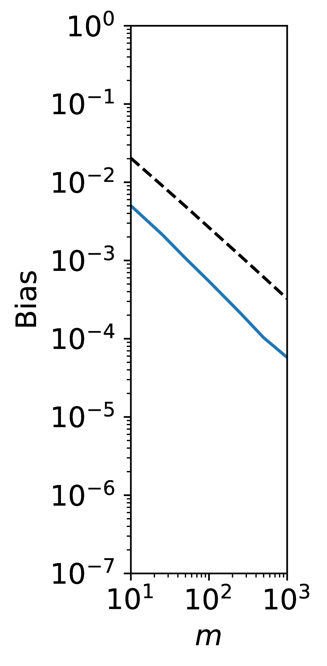
(a)

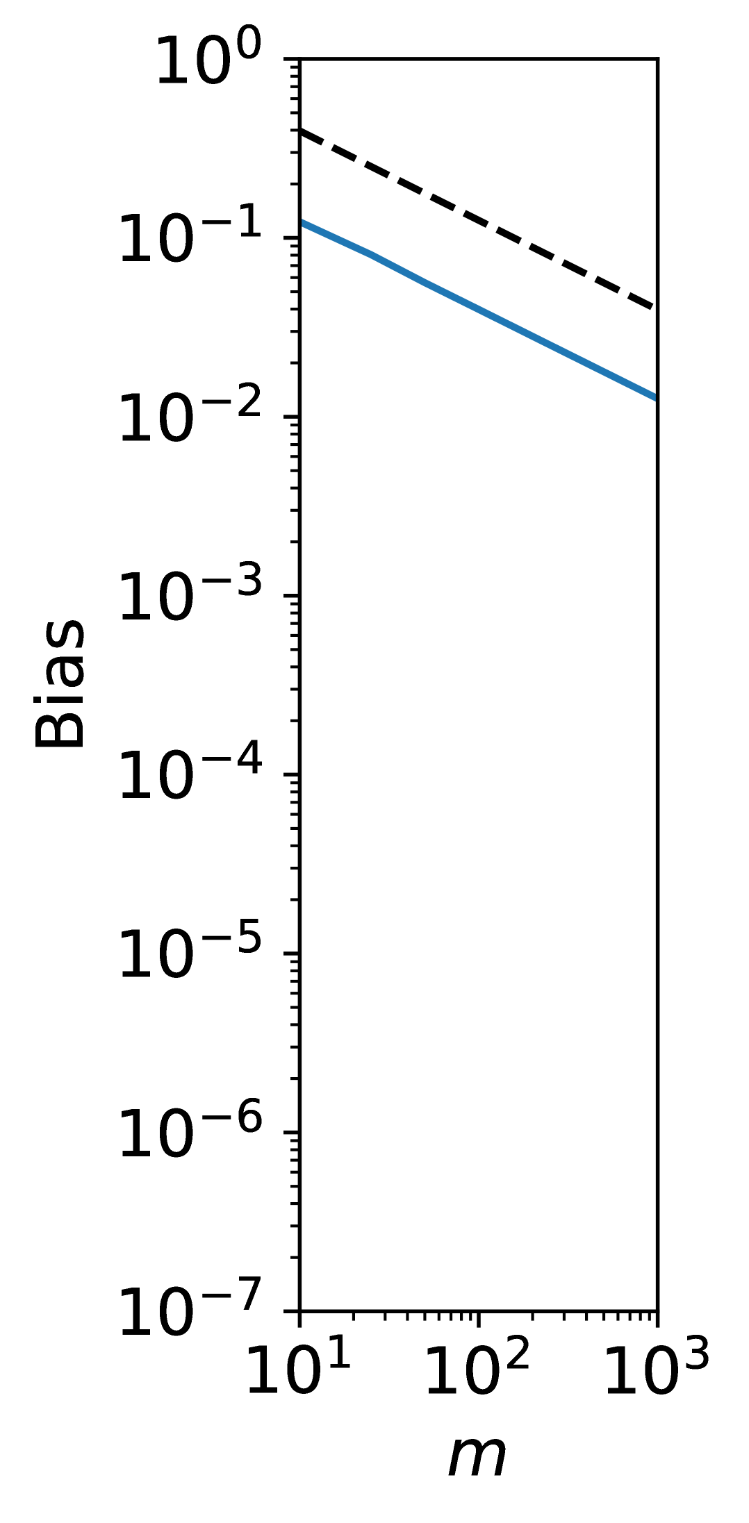
(b)

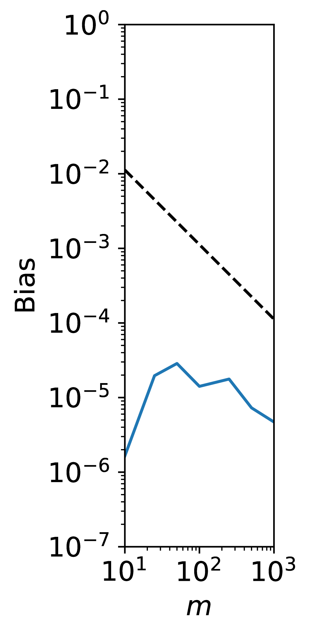
(c)

Figure 7: The bias of the hard-label-based estimator $\widehat{\mathrm{Err}^{*}}\left({\widehat{\eta}_{1:n}}\right)$ as a function of the number $m$ of hard labels per sample. The blue solid lines indicate the experimental results while the black dashed lines indicate the theoretical upper bounds in Theorem˜1.

Appendix C Supplementary for Section˜3

In this section, we present the proof of Theorem˜2. Section˜C.1 presents a new risk bound for binary isotonic regression (Proposition˜4) as well as a useful lemma for general shape-constrained nonparametric regression problems (Lemma˜6). Then, we employ these results to prove the theorem in Section˜C.2.

C.1 Risk bound for binary isotonic regression

C.1.1 Nonparametric regression and isotonic regression

Here, we introduce general nonparametric regression problems where we aim to estimate the underlying signal from noisy observations. Then, we describe the isotonic regression setting.

Let $T$ be a set. Assume that, for each design point $t_{i}\in T$, $i=1,\ldots,n$, we observe

$$y_{i}=f^{*}(t_{i})+\xi_{i}\text{,}$$ (80)

where $f^{*}:T\to\mathbb{R}$ is the unknown regression function and $\xi_{i}\in\mathbb{R}$ are independent and mean-zero noise variables. A natural estimator would be the least squares estimator (LSE)

$$\widehat{f}\in\operatorname*{\mathrm{arg}\,\mathrm{min}}_{f\in\mathcal{F}}\frac{1}{n}\sum_{i=1}^{n}\left({y_{i}-f(t_{i})}\right)^{2}\text{,}$$ (81)

where $\mathcal{F}$ is some pre-defined function class. In the fixed design setting, the quality of an estimator $\widehat{f}$ is evaluated by the $\ell^{2}$ risk

$$\frac{1}{n}\sum_{i=1}^{n}\left({\widehat{f}(t_{i})-f^{*}(t_{i})}\right)^{2}\text{.}$$ (82)

Under this criterion, estimators are evaluated only on the fixed design points $t_{i}$ so estimating the function $f^{*}$ is equivalent to estimating the sequence/vector $\bm{\mu}:=(f^{*}(t_{1}),\ldots,f^{*}(t_{n}))\in\mathbb{R}^{n}$.

From this perspective, the regression problem can be reformulated as follows. Our observation is an $n$-dimensional random vector $\bm{y}=(y_{1},\ldots,y_{n})\in\mathbb{R}^{n}$ of the form

$$\bm{y}=\bm{\mu}+\bm{\xi}\text{.}$$ (83)

Here $\bm{\mu}=(\mu_{1},\ldots,\mu_{n})\in\mathbb{R}^{n}$ is the unknown signal and $\bm{\xi}=(\xi_{1},\ldots,\xi_{n})\in\mathbb{R}^{n}$ is a centered noise vector whose elements are independent. Let $K\subset\mathbb{R}^{n}$ be a closed convex subset from which we choose our estimates, which corresponds to the function class $\mathcal{F}$ in the function estimation formulation described above. Often it is assumed that the true signal $\bm{\mu}$ indeed belongs to $K$. However, in our results in Section˜C.1, we allow model misspecification, i.e., we do not assume $\bm{\mu}\in K$. The LSE $\widehat{\bm{\mu}}$ is the Euclidean projection of $\bm{y}$ onto $K$:

$$\widehat{\bm{\mu}}=\operatorname*{\mathrm{arg}\,\mathrm{min}}_{\bm{u}\in K}\lVert{\bm{y}-\bm{u}}\rVert_{2}^{2}\text{.}$$ (84)

Isotonic regression Isotonic regression is a special case where we choose $K$ to be the collection $\mathcal{M}_{n}$ of all non-decreasing sequences of length $n$:

$$\mathcal{M}_{n}:=\left\{{\bm{u}\in\mathbb{R}^{n}\mid u_{1}\leq\ldots\leq u_{n}}\right\}\text{.}$$ (85)

Note that $\mathcal{M}_{n}$ is a closed convex cone. Here the goal is to estimate isotonic, or monotonic, signals from noisy observations. Recall that the LSE $\widehat{\bm{\mu}}$ is the Euclidean projection of the observation vector $\bm{y}$ onto $\mathcal{M}_{n}$:

$$\widehat{\bm{\mu}}=\operatorname*{\mathrm{arg}\,\mathrm{min}}_{\bm{u}\in\mathcal{M}_{n}}\lVert{\bm{y}-\bm{u}}\rVert_{2}^{2}\text{.}$$ (86)

It has the following explicit representation (Robertson et al., 1988), which is known as the min-max formula:

$$\widehat{\mu}_{i}=\min_{l\geq i}\max_{k\leq i}\bar{y}_{k:l}\text{,}\quad i=1,\ldots,n\text{,}$$ (87)

where $\bar{y}_{k:l}:=\frac{1}{l-k+1}\sum_{i=k}^{l}y_{i}$ is the average of $y_{k},\ldots,y_{l}$. It can be efficiently computed with the pool adjacent violators (PAV) algorithm (Ayer et al., 1955).

We are interested in evaluating the risk $\frac{1}{n}\lVert{\widehat{\bm{\mu}}-\bm{\mu}}\rVert_{2}^{2}$ of the LSE $\widehat{\bm{\mu}}$, which has been extensively studied in the literature (e.g. Zhang, 2002; Chatterjee, 2014; Chatterjee et al., 2015; Bellec and Tsybakov, 2015; Bellec, 2018; Yang and Barber, 2019; Chatterjee and Lafferty, 2019). We will cover the results from these existing works later in Section˜C.1.2.

C.1.2 Review of the existing risk bounds for isotonic regression

First, we introduce some notions that will be needed below. For each non-decreasing sequence $\bm{u}\in\mathcal{M}_{n}$, we denote its total variation by

$$V(\bm{u}):=\max_{i}u_{i}-\min_{i}u_{i}\text{.}$$ (88)

We also let $k(\bm{u})$ be the number of constant pieces in $\bm{u}$. In other words, $k(\bm{u})-1$ is the number of the inequalities $u_{i}\leq u_{i+1}$ that are strict, so the sequence $u_{1},\ldots,u_{n}$ has $k(\bm{u})-1$ jumps in total.

For the cases where $\bm{\mu}\in\mathcal{M}_{n}$ and the noises have bounded variance $\operatorname*{\mathbb{E}}\left[{\xi_{i}^{2}}\right]\leq\sigma^{2}$, the following bound on the expected risk was proven by Zhang (2002):

$$\operatorname*{\mathbb{E}}\left[{\frac{1}{n}\lVert{\widehat{\bm{\mu}}-\bm{\mu}}\rVert_{2}^{2}}\right]\leq C\left\{{\left({\frac{\sigma^{2}V(\bm{\mu})}{n}}\right)^{2/3}+\frac{\sigma^{2}\log(en)}{n}}\right\}\text{,}$$ (89)

where $C\leq 12.3$ is an absolute constant. Chatterjee et al. (2015) showed this $n^{-2/3}$ rate is minimax, while providing another type of risk bound

$$\operatorname*{\mathbb{E}}\left[{\frac{1}{n}\lVert{\widehat{\bm{\mu}}-\bm{\mu}}\rVert_{2}^{2}}\right]\leq 6\min_{\bm{u}\in\mathcal{M}_{n}}\left\{{\frac{1}{n}\lVert{\bm{u}-\bm{\mu}}\rVert_{2}^{2}+\frac{\sigma^{2}k(\bm{u})}{n}\log\frac{en}{k(\bm{u})}}\right\}$$ (90)

under the assumptions that $\bm{\mu}\in\mathcal{M}_{n}$ and $\xi_{i}$ are i.i.d. with finite variance $\operatorname*{\mathbb{E}}\left[{\xi_{i}^{2}}\right]=\sigma^{2}$. (90) is adaptive, unlike (89), in the sense that it gives a parametric rate $n^{-1/2}$ up to logarithmic factors when the true signal $\bm{\mu}$ is well-approximated by some $\bm{u}\in\mathcal{M}_{n}$ with small $k(\bm{u})$ (i.e., a piecewise constant sequence with not too many pieces). Later, Bellec (2018) showed two types of bounds, improving the previous results in the case of i.i.d. Gaussian noise $\bm{\xi}\sim N(0,\sigma^{2}I_{n})$. In the first result, they proved that, with probability greater than $1-e^{-x}$, we have

$$\frac{1}{n}\lVert{\widehat{\bm{\mu}}-\bm{\mu}}\rVert_{2}^{2}\leq\min_{\bm{u}\in\mathcal{M}_{n}}\left\{{\frac{1}{n}\lVert{\bm{u}-\bm{\mu}}\rVert_{2}^{2}+2c\sigma^{2}\left({\frac{\sigma+V(\bm{u})}{\sigma n}}\right)^{2/3}}\right\}+\frac{4\sigma^{2}x}{n}\text{,}$$ (91)

where $c$ is an absolute constant. A corresponding bound in expectation also can be derived by integrating this high-probability bound. The second result is that, with probability at least $1-e^{-x}$, we have

$$\frac{1}{n}\lVert{\widehat{\bm{\mu}}-\bm{\mu}}\rVert_{2}^{2}\leq\min_{\bm{u}\in\mathcal{M}_{n}}\left\{{\frac{1}{n}\lVert{\bm{u}-\bm{\mu}}\rVert_{2}^{2}+\frac{2\sigma^{2}k(\bm{u})}{n}\log\frac{en}{k(\bm{u})}}\right\}+\frac{4\sigma^{2}x}{n}\text{.}$$ (92)

A similar in-expectation bound

$$\operatorname*{\mathbb{E}}\left[{\frac{1}{n}\lVert{\widehat{\bm{\mu}}-\bm{\mu}}\rVert_{2}^{2}}\right]\leq\min_{\bm{u}\in\mathcal{M}_{n}}\left\{{\frac{1}{n}\lVert{\bm{u}-\bm{\mu}}\rVert_{2}^{2}+\frac{\sigma^{2}k(\bm{u})}{n}\log\frac{en}{k(\bm{u})}}\right\}$$ (93)

also holds. Bellec (2018)’s results, (91), (92) and (93), have several features worth mentioning. First, their leading constants are $1$. For this reason, these bounds are called sharp oracle inequalities. Second, they are valid even under model misspecification, which (89) nor (90) allowed. Third, (91) and (92) were the first oracle inequalities that were shown to hold with high probability, rather than in expectation. The last point is especially important for our purpose, i.e., computing confidence intervals. A major drawback of the results by Bellec (2018) is that they are restricted to Gaussian noise. Yang and Barber (2019) employed their unique sliding window norm technique to prove the following bound for general sub-Gaussian noise with variance proxy $\sigma^{2}$:

$$\operatorname*{\mathbb{E}}\left[{\frac{1}{n}\lVert{\widehat{\bm{\mu}}-\bm{\mu}}\rVert_{2}^{2}}\right]\leq 48\left({\frac{\sigma^{2}V(\bm{\mu})\log(2n)}{n}}\right)^{2/3}+\frac{96\sigma^{2}\log^{2}(2n)}{n}$$ (94)

Under model misspecification $\bm{\mu}\not\in\mathcal{M}_{n}$, (94) still remains valid with $\bm{\mu}$ replaced by its projection onto $\mathcal{M}_{n}$. A similar high-probability bound also can be derived by almost the same argument, although they did not mention it in their paper.

C.1.3 Metric entropy bounds for isotonic constraints

For real numbers $-\infty<a<b<\infty$, we define the truncated version of the isotonic cone $\mathcal{M}_{n}$ as

$$\mathcal{M}_{n}(a,b):=\left\{{\bm{x}\in\mathbb{R}^{n}\mid a\leq x_{1}\leq\ldots\leq x_{n}\leq b}\right\}\text{.}$$ (95)

$\mathcal{M}_{n}(a,b)$ is not a cone, unlike $\mathcal{M}_{n}$, but it is still a closed convex set. We also define the set of all non-decreasing functions from $[0,1)$ to $[0,1]$:

$$\mathcal{M}:=\left\{{f:[0,1)\to[0,1]\mid\text{$f$ is non-decreasing}}\right\}\text{.}$$ (96)

Let $(\mathcal{F},\lVert{\cdot}\rVert)$ be a subset of a normed function space. Given two functions $l,u\in\mathcal{F}$ with $\lVert{u-l}\rVert\leq\varepsilon$, the set

$$\left\{{f\in\mathcal{F}\mid l\leq f\leq u}\right\}$$ (97)

is called an $\varepsilon$-bracket (Van Der Vaart and Wellner, 1996). The $\varepsilon$-bracketing number $\mathcal{N}_{[\,]}(\mathcal{F},\lVert{\cdot}\rVert,\varepsilon)$ of $(\mathcal{F},\lVert{\cdot}\rVert)$ is the smallest number of $\varepsilon$-brackets needed to cover $\mathcal{F}$. The logarithm of bracketing numbers is called bracketing entropy.

Van Der Vaart and Wellner (1996, Theorem 2.7.5) and Gao and Wellner (2007, Theorem 1.1) proved the $\varepsilon$-bracketing entropy of $\mathcal{M}$ is of order $\varepsilon^{-1}$, i.e.,

$$\log\mathcal{N}_{[\,]}(\mathcal{M},\lVert{\cdot}\rVert_{L^{p}},\varepsilon)\leq\frac{C_{p}}{\varepsilon}\text{,}\quad\forall\varepsilon>0\text{,}$$ (98)

where $C_{p}>0$ is a universal constant depending only on $p\in[1,\infty)$ and $\lVert{\cdot}\rVert_{L^{p}}$ is the $L^{p}$ norm under Lebesgue measure. Later, Chatterjee (2014, Lemma 4.20) established a tool that enables us to convert the bracketing entropy bound (98) for monotone functions into a metric entropy bound for monotone sequences. It has been commonly utilized in previous studies (Chatterjee, 2014; Bellec, 2018; Chatterjee and Lafferty, 2019). Although the original result by Chatterjee (2014) was stated for the Euclidean norm $\lVert{\cdot}\rVert_{2}$, results for other $p$-norms $\lVert{\cdot}\rVert_{p},\ p\in[1,\infty]$ can be obtained by a similar argument. We state and prove this generalized version below.

Theorem 4.

Take any $p\in[1,\infty)$. Then, we have

$$\log\mathcal{N}(\mathcal{M}_{n}(a,b),\lVert{\cdot}\rVert_{p},\varepsilon)\leq\frac{C_{p}(b-a)n^{1/p}}{\varepsilon}$$ (99)

for $\varepsilon>0$. Here $C_{p}$ is the same constant as in (98).

Proof.

Without loss of generality, we assume $a=0$ and $b=1$. First of all, note the general fact that $\varepsilon$-covering number is upper-bounded by $2\varepsilon$-bracketing number (see, e.g. Van Der Vaart and Wellner, 1996). This, together with the bracketing number bound (98), implies

$$\log\mathcal{N}(\mathcal{M},\lVert{\cdot}\rVert_{L^{p}},\varepsilon)\leq\log\mathcal{N}_{[\,]}(\mathcal{M},\lVert{\cdot}\rVert_{L^{p}},2\varepsilon)\leq\frac{C_{p}}{2\varepsilon}\text{.}$$ (100)

Therefore, there exists an $\varepsilon$-net $\tilde{N}$ of the function class $\mathcal{M}$ with $\log\lvert\tilde{N}\rvert\leq\frac{C_{p}}{2\varepsilon}$. Now set $\delta=2n^{1/p}\varepsilon$. We will construct a $\delta$-net $N$ of the sequence class $\mathcal{M}_{n}(0,1)$ based on $\tilde{N}$. To this end, for each monotone sequence $\bm{u}\in\mathcal{M}_{n}(0,1)$, we associate it with a monotone piecewise constant function $g_{\bm{u}}\in\mathcal{M}$ of the form

$$g_{\bm{u}}(x)=\sum_{i=1}^{n}u_{i}\mathbbm{1}\left[{x\in\left[\frac{i-1}{n},\frac{i}{n}\right)}\right]\text{.}$$ (101)

For each $f\in\tilde{N}$, we check if $f$ can be approximated by $g_{\bm{u}}$ for some $\bm{u}\in\mathcal{M}_{n}(0,1)$ so that $\lVert{f-g_{\bm{u}}}\rVert_{L^{p}}\leq\varepsilon$. If it can, we put one of the corresponding sequences $\bm{u}$ into $N$. By construction of $N$, we have $\log\left\lvert{N}\right\rvert\leq\log\lvert\tilde{N}\rvert\leq\frac{C_{p}}{2\varepsilon}$.

Next, we confirm $N$ is indeed a $\delta$-net of $\mathcal{M}_{n}(0,1)$. Take any $\bm{u}\in\mathcal{M}_{n}(0,1)$. Then, since $\tilde{N}$ is a $\varepsilon$-net of $\mathcal{M}$ and $g_{\bm{u}}$ belongs to $\mathcal{M}$, there exists $f\in\tilde{N}$ approximating $g_{\bm{u}}$ so that

$$\lVert{g_{\bm{u}}-f}\rVert_{L^{p}}\leq\varepsilon\text{.}$$ (102)

Now, observe that (102) implies “$f\in\tilde{N}$ can be approximated by $g_{\bm{u}}$ for some $\bm{u}\in\mathcal{M}_{n}(0,1)$,” so there is $\bm{v}\in N$ such that $\lVert{f-g_{\bm{v}}}\rVert_{L^{p}}\leq\varepsilon$ by the construction of $N$. So the triangle inequality implies

$$\lVert{g_{\bm{u}}-g_{\bm{v}}}\rVert_{L^{p}}\leq\lVert{g_{\bm{u}}-f}\rVert_{L^{p}}+\lVert{f-g_{\bm{v}}}\rVert_{L^{p}}\leq 2\varepsilon\text{.}$$ (103)

On the other hand, the left-hand side can be explicitly calculated as follows.

$$\lVert{g_{\bm{u}}-g_{\bm{v}}}\rVert_{L^{p}} =\left({\int_{0}^{1}(g_{\bm{u}}-g_{\bm{v}})^{p}}\right)^{1/p}$$

$$=\left({\int_{0}^{1}\sum_{i=1}^{n}(u_{i}-v_{i})^{p}\mathbbm{1}\left[{x\in\left[\frac{i-1}{n},\frac{i}{n}\right)}\right]}\right)^{1/p}$$

$$=\left({\frac{1}{n}\sum_{i=1}^{n}(u_{i}-v_{i}i)^{p}}\right)^{1/p}$$

$$=\frac{\lVert{\bm{u}-\bm{v}}\rVert_{p}}{n^{1/p}}\text{.}$$ (104)

Therefore, it follows that, for any $\bm{u}\in\mathcal{M}_{n}(0,1)$, there exists $\bm{v}\in N$ such that

$$\lVert{\bm{u}-\bm{v}}\rVert_{p}\leq 2n^{1/p}\varepsilon=\delta\text{,}$$ (105)

which proves $N$ is a $\delta$-net of $\mathcal{M}_{n}(0,1)$ with respect to $p$-norm. Thus, we have

$$\log\mathcal{N}(\mathcal{M}_{n}(0,1),\lVert{\cdot}\rVert_{p},\delta)\leq\log\left\lvert{N}\right\rvert\leq\frac{C_{p}}{2\varepsilon}=\frac{C_{p}n^{1/p}}{\delta}\text{.}$$ (106)

∎

C.1.4 Lemma for proving sharp oracle inequalities

Here, we present a general lemma that we can use to prove a sharp oracle inequality for the LSE

$$\widehat{\bm{\mu}}=\operatorname*{\mathrm{arg}\,\mathrm{min}}_{\bm{u}\in K}\lVert{\bm{y}-\bm{u}}\rVert_{2}^{2}=\operatorname*{\mathrm{arg}\,\mathrm{min}}_{\bm{u}\in K}\lVert{(\bm{\mu}+\bm{\xi})-\bm{u}}\rVert_{2}^{2}$$ (107)

under a convex constraint $K\subset\mathbb{R}^{n}$ and a general noise $\bm{\xi}$. Here ‘‘sharp’’ means that the resulting oracle inequality has a leading constant $1$. Lemma˜6 below is a slight extension of the elegant argument given by Bellec (2018, Theorem 2.3), which was given for the i.i.d. Gaussian noise setting. In fact, it is essentially just a deterministic statement, so there is no requirement for the stochastic structure of the noise $\bm{\xi}$. Their key idea was to make use of convexity to obtain a stronger basic inequality than usual. Here basic inequality refers to the elementary fact

$$\lVert{\widehat{\bm{\mu}}-\bm{\mu}}\rVert_{2}^{2}\leq\lVert{\bm{u}-\bm{\mu}}\rVert_{2}^{2}+2\langle\bm{\xi},\widehat{\bm{\mu}}-\bm{u}\rangle\text{,}\quad\forall\bm{u}\in K$$ (108)

that holds even if $K$ is non-convex. (108) immediately follows from the optimality of $\widehat{\bm{\mu}}$, i.e.,

$$\lVert{\bm{y}-\widehat{\bm{\mu}}}\rVert_{2}^{2}\leq\lVert{\bm{y}-\bm{u}}\rVert_{2}^{2}\text{,}\quad\forall\bm{u}\in K\text{.}$$ (109)

Now suppose $K$ is convex. Then, the LSE (i.e., the projection of $\bm{y}$ onto $K$) satisfies the variational inequality

$$\langle\bm{u}-\widehat{\bm{\mu}},\bm{y}-\widehat{\bm{\mu}}\rangle\leq 0\text{,}\quad\forall\bm{u}\in K\text{,}$$ (110)

which is an elementary result of convex geometry. Importantly, it implies

$$\lVert{\bm{y}-\widehat{\bm{\mu}}}\rVert_{2}^{2}\leq\lVert{\bm{y}-\bm{u}}\rVert_{2}^{2}-\lVert{\widehat{\bm{\mu}}-\bm{u}}\rVert_{2}^{2}\text{,}\quad\forall\bm{u}\in K\text{.}$$ (111)

(111) can be seen as a strengthened version of (109) with the additional term $-\lVert{\widehat{\bm{\mu}}-\bm{u}}\rVert_{2}^{2}$. Therefore it can be used to derive a stronger version of the basic inequality (108), i.e.,

$$\lVert{\widehat{\bm{\mu}}-\bm{\mu}}\rVert_{2}^{2}\leq\lVert{\bm{u}-\bm{\mu}}\rVert_{2}^{2}+2\langle\bm{\xi},\widehat{\bm{\mu}}-\bm{u}\rangle-\lVert{\widehat{\bm{\mu}}-\bm{u}}\rVert_{2}^{2}\text{,}\quad\forall\bm{u}\in K$$ (112)

This is the inequality (2.3) in Bellec (2018). Following their method, we use this fact as the starting point of the proof of Lemma˜6. Recall that we do not require $\bm{\mu}$ to belong to $K$. It can be any point in $\mathbb{R}^{n}$, i.e., we allow model misspecification.

Lemma 6 (Localized width and projection).

Take any $p\in[2,\infty]$. Let $\bm{\xi},\bm{\mu}\in\mathbb{R}^{n}$ be arbitrarily fixed vectors and $K\subset\mathbb{R}^{n}$ be a convex set. Suppose that a point $\bm{u}\in K$ and positive numbers $t,s$ satisfy

$$Z(\bm{u},t):=\sup_{\bm{v}\in K,\lVert{\bm{v}-\bm{u}}\rVert_{p}\leq t}\langle\bm{\xi},\bm{v}-\bm{u}\rangle\leq\frac{t^{2}}{2}+ts\text{.}$$ (113)

Then, the projection $\widehat{\bm{\mu}}$ of $\bm{\mu}+\bm{\xi}$ onto $K$ satisfies

$$\lVert{\widehat{\bm{\mu}}-\bm{\mu}}\rVert_{2}^{2}\leq\lVert{\bm{u}-\bm{\mu}}\rVert_{2}^{2}+\left({t+s}\right)^{2}\text{.}$$ (114)

Proof.

For ease of notation, let

$$K_{p}(\bm{u},t):=\left\{{\bm{v}\in K\mid\lVert{\bm{v}-\bm{u}}\rVert_{p}\leq t}\right\}\text{.}$$ (115)

Note that $Z(\bm{u},t)=\sup_{\bm{v}\in K_{p}(\bm{u},t)}\langle\bm{\xi},\bm{v}-\bm{u}\rangle$. We break our analysis into two cases.

1. If $\lVert{\widehat{\bm{\mu}}-\bm{u}}\rVert_{p}\leq t$, then $\widehat{\bm{\mu}}\in K_{p}(\bm{u},t)$. Therefore the basic inequality (112) implies

   $$\lVert{\widehat{\bm{\mu}}-\bm{\mu}}\rVert_{2}^{2}-\lVert{\bm{u}-\bm{\mu}}\rVert_{2}^{2}\leq 2\langle\bm{\xi},\widehat{\bm{\mu}}-\bm{u}\rangle-\lVert{\widehat{\bm{\mu}}-\bm{u}}\rVert_{2}^{2}\leq 2Z(\bm{u},t)-\lVert{\widehat{\bm{\mu}}-\bm{u}}\rVert_{2}^{2}\leq 2Z(\bm{u},t)\text{.}$$ (116)

   Now use the assumption (113) to obtain

   $$\lVert{\widehat{\bm{\mu}}-\bm{\mu}}\rVert_{2}^{2}-\lVert{\bm{u}-\bm{\mu}}\rVert_{2}^{2}\leq t^{2}+2ts\leq\left({t+s}\right)^{2}\text{.}$$ (117)

2. Next, suppose $\lVert{\widehat{\bm{\mu}}-\bm{u}}\rVert_{p}>t$. Letting $\alpha:=t/\lVert{\widehat{\bm{\mu}}-\bm{u}}\rVert_{p}$, we have $\alpha\in(0,1)$. Now take $\bm{v}:=\bm{u}+\alpha(\widehat{\bm{\mu}}-\bm{u})$. Then, the convexity of $K$ implies $\bm{v}\in K$, and clearly, we have $\lVert{\bm{v}-\bm{u}}\rVert_{p}=t$, so $\bm{v}$ is a member of $K_{p}(\bm{u},t)$. Therefore, we can plug $\widehat{\bm{\mu}}-\bm{u}=\alpha^{-1}(\bm{v}-\bm{u})$ into the basic inequality (112) to obtain

   $$\lVert{\widehat{\bm{\mu}}-\bm{\mu}}\rVert_{2}^{2}-\lVert{\bm{u}-\bm{\mu}}\rVert_{2}^{2} \leq 2\langle\bm{\xi},\widehat{\bm{\mu}}-\bm{u}\rangle-\lVert{\widehat{\bm{\mu}}-\bm{u}}\rVert_{2}^{2}$$ (118)

   $$=\frac{2}{\alpha}\langle\bm{\xi},\bm{v}-\bm{u}\rangle-\frac{\lVert{\bm{v}-\bm{u}}\rVert_{2}^{2}}{\alpha^{2}}$$ (119)

   $$\leq\frac{2}{\alpha}Z(\bm{u},t)-\frac{t^{2}}{\alpha^{2}}$$ (120)

   $$=2\frac{Z(\bm{u},t)}{t}\frac{t}{\alpha}-\left({\frac{t}{\alpha}}\right)^{2}$$ (121)

   $$\leq\left({\frac{Z(\bm{u},t)}{t}}\right)^{2}\text{,}$$ (122)

   where we used $\lVert{\bm{v}-\bm{u}}\rVert_{2}^{2}\geq\lVert{\bm{v}-\bm{u}}\rVert_{p}^{2}=t^{2}$ in (120) and $2ab-b^{2}\leq a^{2}$ in (122). Now, the the assumption (113) readily implies

   $$\lVert{\widehat{\bm{\mu}}-\bm{\mu}}\rVert_{2}^{2}-\lVert{\bm{u}-\bm{\mu}}\rVert_{2}^{2}\leq\left({\frac{t}{2}+s}\right)^{2}\leq\left({t+s}\right)^{2}$$ (123)

Therefore the claim is true for both cases. ∎

C.1.5 Risk bound for binary isotonic regression

In the sequel, we apply the general results stated in the previous sections to investigate the binary isotonic regression problem. In binary regression, we are given $n$ binary observations $y_{i}\in\left\{{0,1}\right\}$, each of which is drawn independently from the Bernoulli distribution with mean $\mu_{i}\in[0,1]$. The noise distribution can be described as

$$\operatorname*{\mathbb{P}}\left({\xi_{i}=1-\mu_{i}}\right)=\mu_{i},\quad\operatorname*{\mathbb{P}}\left({\xi_{i}=-\mu_{i}}\right)=1-\mu_{i}\text{.}$$ (124)

Many calibration methods for probabilistic classification, including calibration by isotonic regression (Zadrozny and Elkan, 2002), can be seen as an instance of binary regression problems. Some authors refer to this setup as the Bernoulli model (Yang and Barber, 2019).

To the best of our knowledge, there is no previous work that investigated risk bounds in binary isotonic regression. Here, we derive a new risk bound for this setting. Recall the definitions of the isotonic cone $\mathcal{M}_{n}$ and its truncation $\mathcal{M}_{n}(a,b)$ (see (85) and (95)):

$$\mathcal{M}_{n} =\left\{{\bm{u}\in\mathbb{R}^{n}\mid u_{1}\leq\ldots\leq u_{n}}\right\}\text{,}$$ (125)

$$\mathcal{M}_{n}(a,b) =\left\{{\bm{u}\in\mathbb{R}^{n}\mid a\leq u_{1}\leq\ldots\leq u_{n}\leq b}\right\}\quad(-\infty<a<b<\infty)\text{.}$$ (126)

From the min-max formula (87), one can observe that the unbounded set $\mathcal{M}_{n}$ can be replaced with the bounded closed convex set $\mathcal{M}_{n}(0,1)$ in binary isotonic regression. In other words, the least squares estimator for the binary isotonic regression problem can be written as

$$\widehat{\bm{\mu}}=\operatorname*{\mathrm{arg}\,\mathrm{min}}_{\bm{u}\in\mathcal{M}_{n}(0,1)}\lVert{\bm{y}-\bm{u}}\rVert_{2}^{2}\text{.}$$ (127)

It leads to the following result.

Proposition 4.

With probability at least $1-e^{-x}$, we have

$$\frac{1}{n}\lVert{\widehat{\bm{\mu}}-\bm{\mu}}\rVert_{2}^{2} \leq\min_{\bm{u}\in\mathcal{M}_{n}(0,1)}\frac{1}{n}\lVert{\bm{u}-\bm{\mu}}\rVert_{2}^{2}+\left({\left({\frac{C}{n}}\right)^{1/3}+\sqrt{\frac{2x}{n}}}\right)^{2}\text{,}$$ (128)

where $C$ is an absolute constant.

Remark.

1. Thanks to the replacement of the unbounded set $\mathcal{M}_{n}$ with the bounded set $\mathcal{M}_{n}(0,1)$, we do not have to go through the additional “pealing” step used in Chatterjee (2014) and Chatterjee and Lafferty (2019).

2. This result is valid even under model misspecification.

Proof.

For any $\bm{u}\in\mathcal{M}_{n}(0,1)$ and $t>0$, let

$$K(\bm{u},t) :=\left\{{\bm{v}\in\mathcal{M}_{n}(0,1)\mid\lVert{\bm{v}-\bm{u}}\rVert_{2}\leq t}\right\}\text{,}$$ (129)

$$Z(\bm{u},t) :=\sup_{\bm{v}\in K(\bm{u},t)}\langle\bm{\xi},\bm{v}-\bm{u}\rangle\text{.}$$ (130)

We first control the expectation $\operatorname*{\mathbb{E}}\left[{Z(\bm{u},t)}\right]$. To this end, observe that the process $(X_{\bm{v}})_{\bm{v}\in K(\bm{u},t)}$, where $X_{\bm{v}}:=\langle\bm{\xi},\bm{v}-\bm{u}\rangle$, is a sub-Gaussian process, i.e., for any $\bm{v}_{1},\bm{v}_{2}\in T$, we have $\operatorname*{\mathbb{E}}\left[{X_{\bm{v}_{1}}}\right]=0$ and

$$\log\operatorname*{\mathbb{E}}\left[{e^{\lambda(X_{\bm{v}_{2}}-X_{\bm{v}_{1}})}}\right]\leq\frac{\lambda^{2}\lVert{\bm{v}_{2}-\bm{v}_{1}}\rVert_{2}^{2}}{8}\text{,}\quad\forall\lambda\geq 0\text{.}$$ (131)

Now combining Dudley’s chaining technique (see e.g. van Handel, 2016, Corollary 5.25) and the metric entropy bound in Theorem˜4 gives

$$\operatorname*{\mathbb{E}}\left[{Z(\bm{u},t)}\right] \leq 6\int_{0}^{t}\sqrt{\log\mathcal{N}(K(\bm{u},t),\lVert{\cdot}\rVert_{2},\varepsilon)}\,d\varepsilon$$

$$\leq 6\int_{0}^{t}\sqrt{\frac{C_{2}\sqrt{n}}{\varepsilon}}\,d\varepsilon$$

$$=12C_{2}^{1/2}n^{1/4}t^{1/2}\text{,}$$ (132)

where $C_{2}$ is the constant appearing in (98).

Moreover, it is straightforward to see that, for each fixed $\bm{u}$ and $t$, $Z(\bm{u},t)$ is a convex $t$-Lipschitz function of $\bm{\xi}$. Therefore, by using Theorem 6.10 in Boucheron et al. (2013) together with (132), with probability greater than $1-e^{-x}$, we have

$$Z(\bm{u},t)\leq\operatorname*{\mathbb{E}}\left[{Z(\bm{u},t)}\right]+t\sqrt{2x}\leq 12C_{2}^{1/2}n^{1/4}t^{1/2}+t\sqrt{2x}\text{.}$$ (133)

Now, define $t^{*}:=4(9C_{2})^{1/3}n^{1/6}$ and observe that we have $12C_{2}^{1/2}n^{1/4}t^{1/2}\leq\frac{t^{2}}{2}$ for any $t\geq t^{*}$. Therefore, Lemma˜6 yields

$$\lVert{\widehat{\bm{\mu}}-\bm{\mu}}\rVert_{2}^{2}\leq\lVert{\bm{u}-\bm{\mu}}\rVert_{2}^{2}+\left({t^{*}+\sqrt{2x}}\right)^{2}\leq\left({\lVert{\bm{u}-\bm{\mu}}\rVert_{2}+t^{*}+\sqrt{2x}}\right)^{2}$$ (134)

with probability at least $1-e^{-x}$. we obtain the result by dividing both sides by $n$ and taking the minimum over all $\bm{u}\in\mathcal{M}_{n}(0,1)$. ∎

C.2 Proof of Theorem˜2

We are just one lemma away from proving our main theorem. The following lemma states that the error between the two estimates with different sets of soft labels can be upper bounded by the root-mean-square error between them.

Lemma 7 (restate=binlip, name=).

For any set of soft labels $\left\{{\eta^{\prime}_{i}}\right\}_{i=1}^{n}\in[0,1]^{n}$, it holds that

$$\left\lvert{\widehat{\mathrm{Err}^{*}}(\eta^{\prime}_{1:n})-\widehat{\mathrm{Err}^{*}}(\eta_{1:n})}\right\rvert\leq\dfrac{1}{n}\sum_{i=1}^{n}\left\lvert{\eta^{\prime}_{i}-\eta_{i}}\right\rvert\leq\sqrt{\dfrac{1}{n}\sum_{i=1}^{n}\left({\eta^{\prime}_{i}-\eta_{i}}\right)^{2}}\text{.}$$ (135)

Proof.

Since $x\in[0,1]\mapsto\min\left\{{x,1-x}\right\}$ is $1$-Lipschitz, we have

$$\left\lvert{\widehat{\mathrm{Err}^{*}}(\eta^{\prime}_{1:n})-\widehat{\mathrm{Err}^{*}}(\eta_{1:n})}\right\rvert\leq \frac{1}{n}\sum_{i=1}^{n}\left\lvert{\min\left\{{\eta^{\prime}_{i},1-\eta^{\prime}_{i}}\right\}-\min\left\{{\eta_{i},1-\eta_{i}}\right\}}\right\rvert$$ (136)

$$\leq \frac{1}{n}\sum_{i=1}^{n}\left\lvert{\eta^{\prime}_{i}-\eta_{i}}\right\rvert\text{.}$$ (137)

The second inequality follows from Jensen’s inequality.

∎

We can finally prove the theorem.

Proof.

By the triangle inequality, we have

$$\left\lvert{\widehat{\mathrm{Err}^{*}}(\widehat{\eta}_{1:n}^{\mathrm{iso}})-\mathrm{Err}^{*}}\right\rvert\leq\left\lvert{\widehat{\mathrm{Err}^{*}}(\widehat{\eta}_{1:n}^{\mathrm{iso}})-\widehat{\mathrm{Err}^{*}}(\eta_{1:n})}\right\rvert+\left\lvert{\widehat{\mathrm{Err}^{*}}(\eta_{1:n})-\mathrm{Err}^{*}}\right\rvert\text{.}$$ (138)

Using Lemma˜7 for the first term and Proposition 3.2 of Ishida et al. (2023) for the second term, we have

$$\left\lvert{\widehat{\mathrm{Err}^{*}}(\widehat{\eta}_{1:n}^{\mathrm{iso}})-\mathrm{Err}^{*}}\right\rvert\leq\sqrt{\dfrac{1}{n}\sum_{i=1}^{n}\left({\widehat{\eta}_{i}^{\mathrm{iso}}-\eta_{i}}\right)^{2}}+\sqrt{\frac{\log(4/\delta)}{8n}}$$ (139)

with probability at least $1-\delta/2$. Now, we evaluate the first term on the right-hand side by applying Proposition˜4 for $\bm{\mu}=(\eta_{(1)},\dots,\eta_{(n)})$. Conditioned on $\left\{{x_{i}}\right\}_{i=1}^{n}$, with probability at least $1-\delta/2$, we have

$$\dfrac{1}{n}\sum_{i=1}^{n}\left({\widehat{\eta}_{i}^{\mathrm{iso}}-\eta_{i}}\right)^{2}\leq\min_{\bm{u}\in\mathcal{M}_{n}(0,1)}\dfrac{1}{n}\sum_{i=1}^{n}\left({u_{i}-\eta_{(i)}}\right)^{2}+\left({\left({\frac{C}{n}}\right)^{1/3}+\sqrt{\frac{2\log(2/\delta)}{n}}}\right)^{2}\text{.}$$ (140)

Since $f$ is increasing and $\tilde{\eta}_{(1)}=f(\eta_{(1)})\leq\dots\leq\tilde{\eta}_{(n)}=f(\eta_{(n)})$, we have $\eta_{(1)}\leq\dots\leq\eta_{(n)}$, i.e., $(\eta_{(1)},\dots,\eta_{(n)})\in\mathcal{M}_{n}$. Therefore, $\min_{\bm{u}\in\mathcal{M}_{n}(0,1)}\frac{1}{n}\sum_{i=1}^{n}\left({u_{i}-\eta_{(i)}}\right)^{2}$ is zero as we can choose $\bm{u}=(\eta_{(1)},\dots,\eta_{(n)})$. As a result, we have

$$\sqrt{\dfrac{1}{n}\sum_{i=1}^{n}\left({\widehat{\eta}_{i}^{\mathrm{iso}}-\eta_{i}}\right)^{2}}\leq\left({\frac{C}{n}}\right)^{1/3}+\sqrt{\frac{2\log(2/\delta)}{n}}\text{.}$$ (141)

Plugging (141) into (139) and rewriting $C^{1/3}$ as $C$, we have

$$\left\lvert{\widehat{\mathrm{Err}^{*}}(\widehat{\eta}_{1:n}^{\mathrm{iso}})-\mathrm{Err}^{*}}\right\rvert\leq\frac{C}{n^{1/3}}+2\sqrt{\frac{2\log(2/\delta)}{n}}$$ (142)

with probability at least $1-\delta$. ∎

Appendix D Supplementary for Section˜4

D.1 Experimental details

We utilized the scikit-learn library (Pedregosa et al., 2011), version 1.6.1, for isotonic regression. We used the implementation of the histogram binning algorithm provided by the uncertainty-calibration package (version 0.1.4; Kumar et al., 2019). We employed the beta-calibration implementation provided in the betacal package (version 1.1.0; Kull et al., 2017). We used the bootstrap function from the SciPy library (Virtanen et al., 2020), version 1.15.3, to obtain 95% bootstrap confidence intervals. For each estimation method, the experiment took around 20--30 minutes on a CPU. The details of the computational resources used can be found in Appendix˜E.

For the sake of comparison in Figure˜4(c), we trained a ResNet-18 (He et al., 2016) on Fashion-MNIST for 100 epochs with a batch size of 128 using the Adam optimizer with a learning rate of 0.001. It took less than an hour.

D.2 Corruption parameters

In experiments with synthetic mixture-of-gaussians data, we used the following corruption function:

$$f(p;a,b)=\left({1+\left({\frac{1-p}{p}}\right)^{1/a}\frac{1-b}{b}}\right)^{-1}\text{,}\ 0<p<1,\ a\geq 0,\ 0<b<1\text{.}$$ (143)

Figure˜8 shows the graph of $f(p;a,b)$ for various values of the parameters $a$ and $b$. As you can see, the parameter $a$ makes the soft labels over-confident when $a<1$, leading to an underestimation of the Bayes error, and under-confident when $a>1$, causing an overestimation. On the other hand, setting $b$ to values other than $0.5$ results in asymmetric, skewed corruption.

We conducted the same experiment as in Figure˜4(a) for various values of $a$ and $b$. The results are shown in Figure˜9. Our calibration-based estimators consistently succeed in preventing over- or underestimation of the Bayes error across all sets of parameter values.

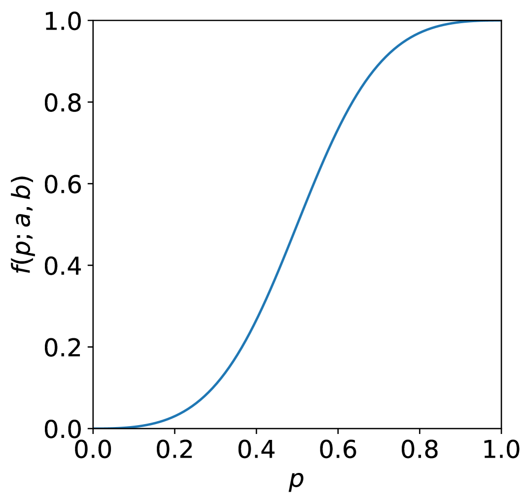
(a) $a=0.4,\ b=0.5$

(b) $a=2,\ b=0.5$

(c) $a=0.4,\ b=0.7$

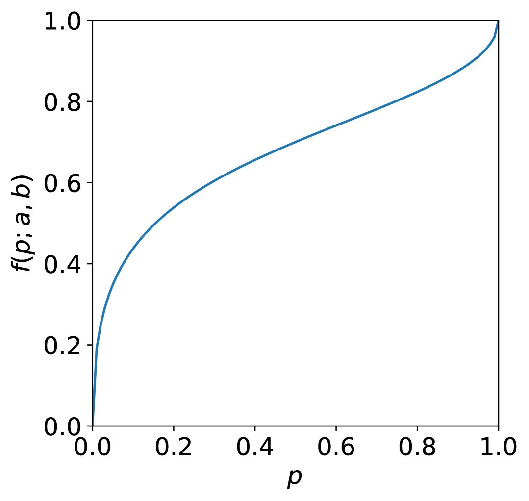
(d) $a=2,\ b=0.7$

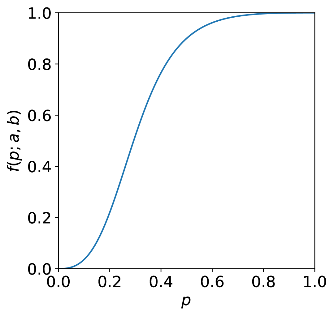
(e) $a=0.4,\ b=0.9$

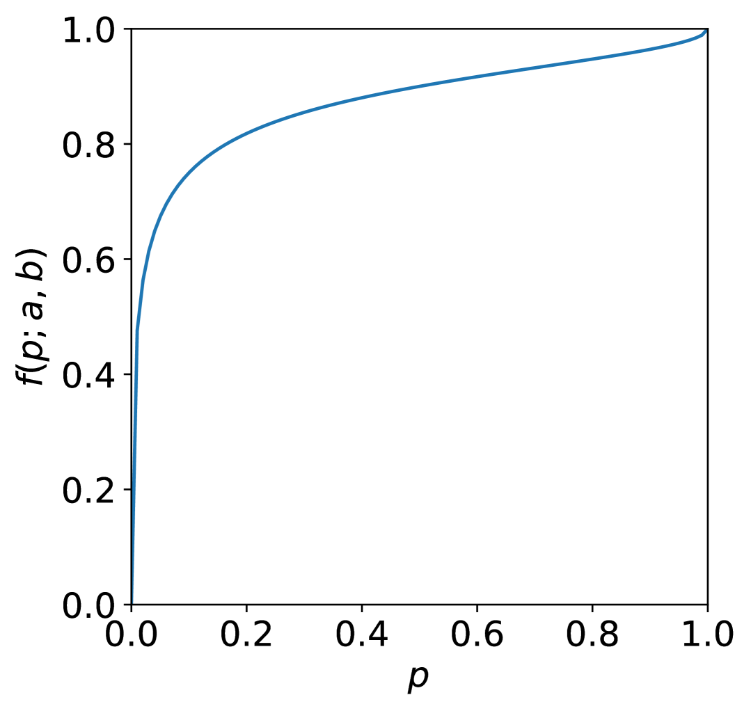
(f) $a=2,\ b=0.9$

Figure 8: The corruption function $f(p;a,b)$ for various parameters $a$ and $b$.

(a) $a=0.4,\ b=0.5$

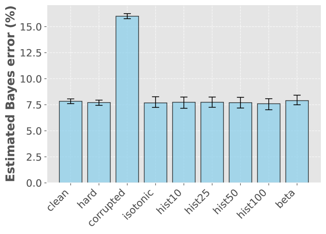
(b) $a=2,\ b=0.5$

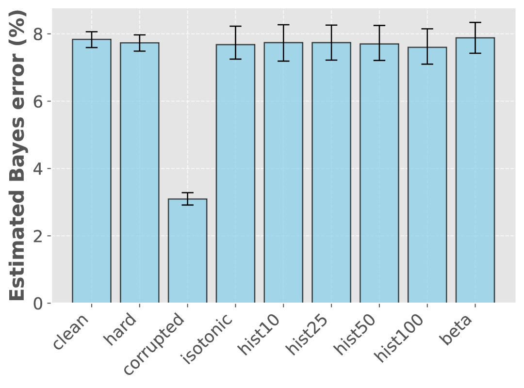
(c) $a=0.4,\ b=0.7$

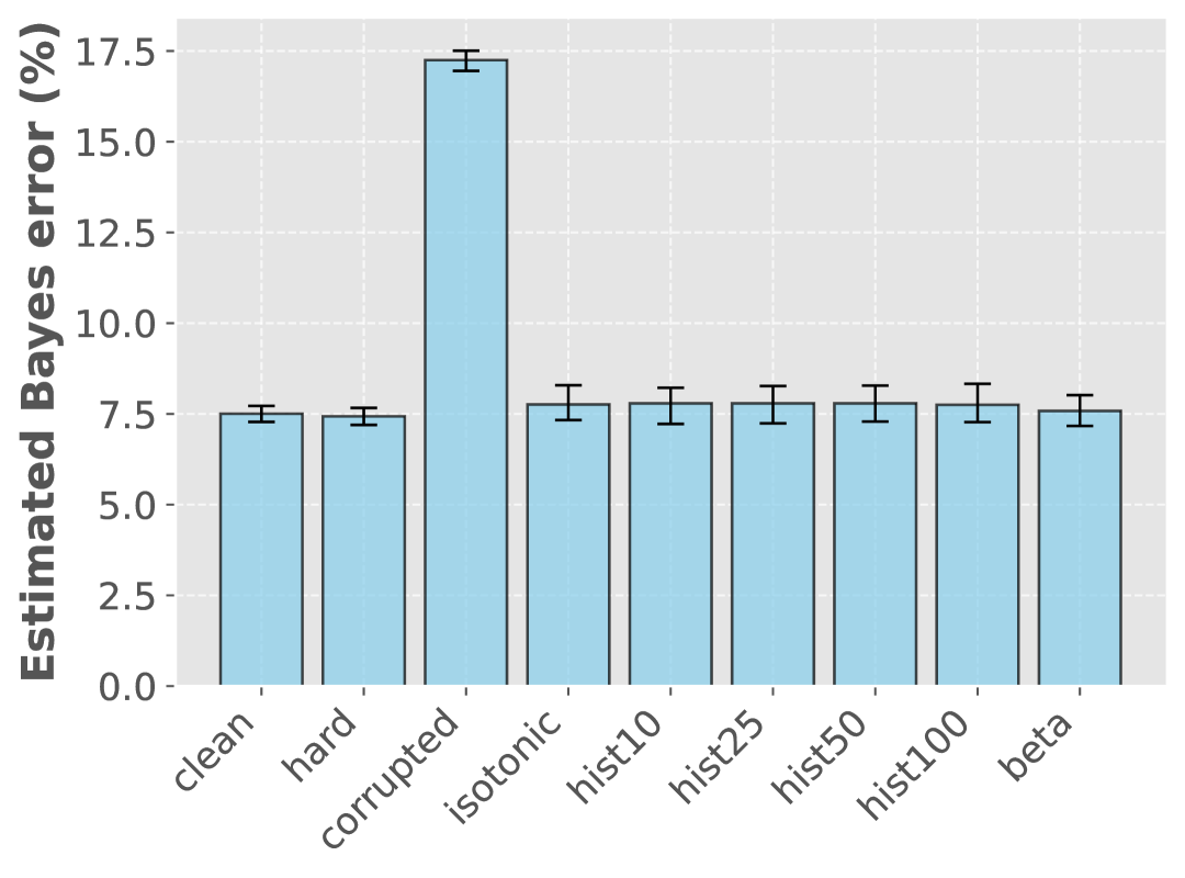
(d) $a=2,\ b=0.7$

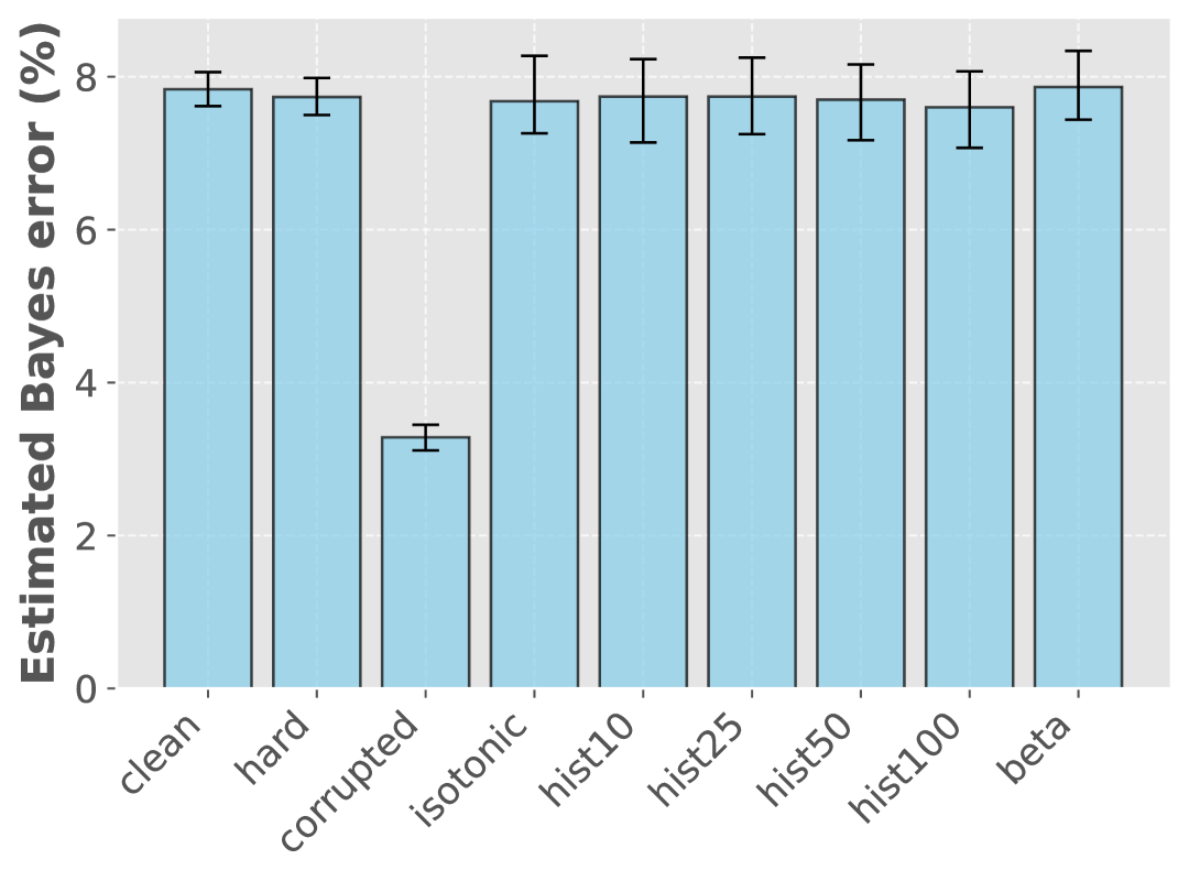
(e) $a=0.4,\ b=0.9$

(f) $a=2,\ b=0.9$

Figure 9: The estimated Bayes error for the synthetic dataset with various corruption parameters $a$ and $b$.

D.3 Violation of the assumption of Theorem˜2

In Section˜3, we presented a theoretical guarantee (Theorem˜2) for our Bayes error estimator based on isotonic calibration. This guarantee assumes that the corruption acting on the soft labels is order-preserving (monotonic). Theoretically, it is still unclear what happens when this assumption is violated. Here we empirically investigate the effects of a departure from monotonicity using synthetic data.

D.3.1 Experimental settings

We draw $n=10000$ data points $\{x_{i}\}^{n}_{i=1}$ from a Gaussian mixture $\mathbb{P}_{\mathcal{X}}=0.6\cdot\mathbb{P}_{0}+0.4\cdot\mathbb{P}_{1}$, where $\mathbb{P}_{0}=N\left({(0,0),I_{2}}\right)$, $\mathbb{P}_{1}=N\left({(2,2),I_{2}}\right)$. For each data point $x_{i}$, we generate its soft label $\tilde{\eta}_{i}$ by sampling $m=3,5,10,25,50,100$ hard labels from the corrupted posterior distribution $\mathrm{Bern}(f(\eta(x_{i});a,b))$ and taking their average. In other words, we obtain the soft label for $x_{i}$ as a draw from $\mathrm{Binom}(m,f(\eta(x_{i});a,b))$ divided by $m$. by drawing from $\mathrm{Binom}(m,f(\eta(x_{i});a,b))$ and dividing the result by $m$. This way, we can create different levels of corruption: although the posterior mean $f(\eta(x_{i});a,b)$ is increasing with respect to the clean soft label $\eta(x_{i})$, the stochasticity of $m$ hard labels adds some noise, which will result in order-breaking corruption. The smaller $m$ gets, the greater the extent of order breakage will be. We consider two sets of corruption parameters: $(a,b)=(2,0.5)$ and $(a,b)=(0.4,0.5)$. Then, we estimate the Bayes error from these corrupted soft labels $\left\{{\tilde{\eta}_{i}}\right\}_{i=1}^{n}$ using the following methods (which we used in Section˜4.1):

1. corrupted: the estimator with corrupted soft labels, i.e., $\widehat{\mathrm{Err}^{*}}\left({\tilde{\eta}_{1:n}}\right)$.

2. The estimator with soft labels obtained by calibrating the corrupted soft labels. We use the following calibration algorithms: isotonic calibration (isotonic), uniform-mass histogram binning with $10,25,50$ and $100$ bins (hist10, hist25, hist50 and hist100), and beta calibration (beta).

As in Section˜4, we use $1000$ bootstrap resamples to compute a 95% confidence interval for each method.

In order to quantify the extent of violation, we use Spearman’s rank correlation coefficient $\rho$ between clean soft labels $\left\{{\eta(x_{i})}\right\}_{i=1}^{n}$ and corrupted soft labels $\left\{{\tilde{\eta}_{i}}\right\}_{i=1}^{n}$. Spearman’s rank correlation coefficient is a non-parametric measure of monotonicity between two variables. It takes values between $-1$ and $+1$. $\rho>0$ means one variable tends to increase as another increases, and $\rho<0$ means the opposite. If $\rho=\pm 1$, the relationship between the two variables is perfectly monotonic. We calculate $\rho$ using the spearmanr function from the SciPy library.

D.3.2 Results

Figure˜10 shows the estimated Bayes error for various levels of order-breaking corruption. The black dashed lines indicate the Bayes error estimated with clean soft labels, which is expected to be a good approximation of the true Bayes error. All the non-parametric calibration methods (isotonic and hist*) perform similarly. However, parametric beta calibration (beta) performs poorly. Particularly, when uncalibrated soft labels are over-confident (i.e., $a=0.4,\ b=0.5$), the more we add hard labels per data point and the more order-preserving the corruption becomes, the worse the estimation performance gets. In the large-$m$ (i.e., large-$\rho$) regime, beta calibration goes ‘‘too far’’ and consistently overestimates the Bayes error. Moreover, it performs poorly for small $\rho$ when uncalibrated soft labels are under-confident ($a=2,\ b=0.5$). This result suggests that isotonic calibration and histogram binning are relatively robust to order-breaking corruption, whereas beta calibration might not be suitable in some cases, especially when uncalibrated soft labels are over-confident.

Interestingly, corrupted’s performance becomes worse as the number $m$ of hard labels per data point increases when $(a,b)=(2,0.5)$. This would be because, as we sample more hard labels, the resulting soft labels are pulled towards the corrupted posterior mean, which makes them more biased. This result highlights the need to calibrate soft labels.

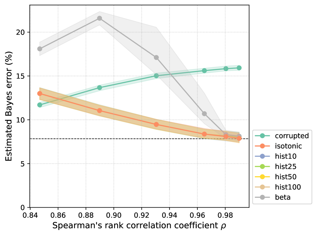
(a) $a=2,\ b=0.5$

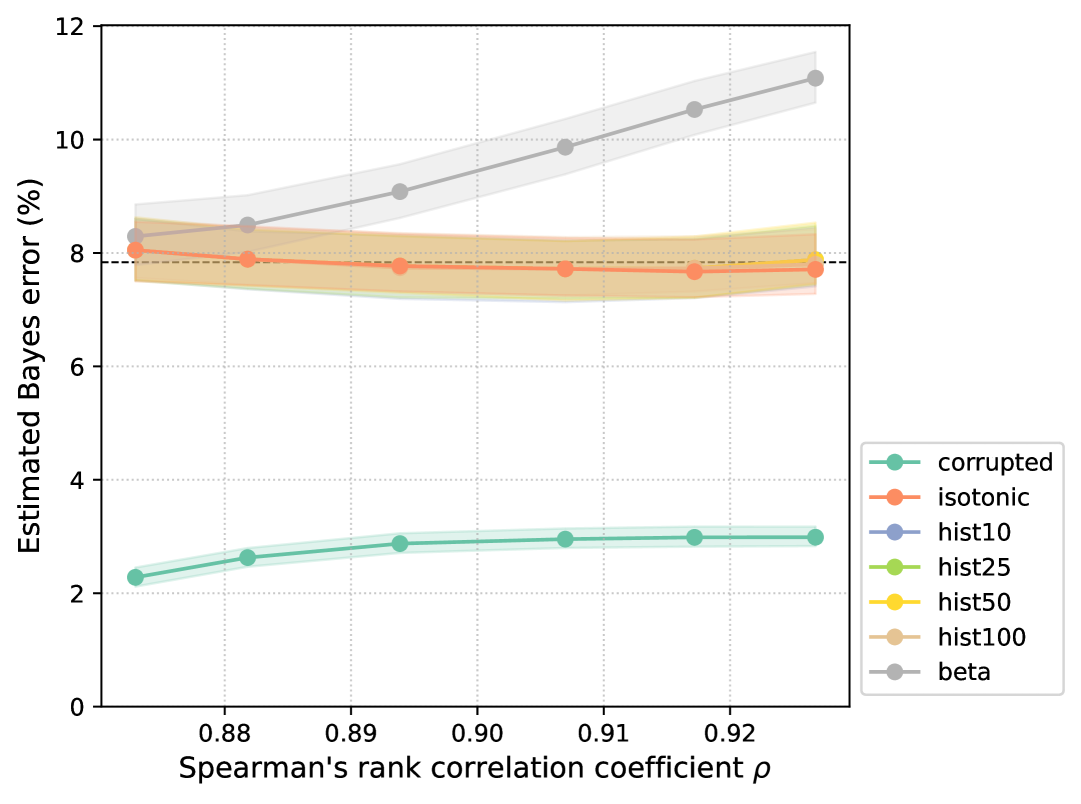
(b) $a=0.4,\ b=0.5$

Figure 10: The Bayes error estimated by directly using corrupted soft labels (corrupted) and by calibrating them (others) for various levels of order-breaking corruption. The 95% bootstrap confident intervals are shown as shaded regions around each line. The black dashed lines indicate the Bayes error estimated with clean soft labels, which is expected to be a good approximation of the true Bayes error.

Appendix E Experiments compute resources

Our experiments do not require any special computer resouces. All of them were conducted on the CPU of a single Apple MacBook Pro (M1 chip, 16GB RAM) except for the ResNet training (see Section˜D.1), where we used a T4 GPU on Google Colab.

References

- Agahi (2021) Hamzeh Agahi. On Jensen’s gap by Taylor’s theorem. Mathematical Methods in the Applied Sciences, 44(14):11565--11570, 2021.
- Argyle et al. (2023) Lisa P Argyle, Ethan C Busby, Nancy Fulda, Joshua R Gubler, Christopher Rytting, and David Wingate. Out of one, many: Using language models to simulate human samples. Political Analysis, 31(3):337--351, 2023.
- Ayer et al. (1955) Miriam Ayer, H. Daniel Brunk, George M. Ewing, William T. Reid, and Edward Silverman. An empirical distribution function for sampling with incomplete information. The Annals of Mathematical Statistics, pages 641--647, 1955.
- Becker (2012) Robert A. Becker. The variance drain and Jensen’s inequality. Technical report, CAEPR Working Paper, 2012.
- Bellec (2018) Pierre C. Bellec. Sharp oracle inequalities for least squares estimators in shape restricted regression. The Annals of Statistics, 46(2):745--780, 2018.
- Bellec and Tsybakov (2015) Pierre C. Bellec and Alexandre B. Tsybakov. Sharp oracle bounds for monotone and convex regression through aggregation. The Journal of Machine Learning Research, 16:1879--1892, 2015.
- Berisha et al. (2014) Visar Berisha, Alan Wisler, Alfred O. Hero, and Andreas Spanias. Empirically estimable classification bounds based on a new divergence measure. arXiv preprint arXiv:1412.6534, 2014.
- Boucheron et al. (2013) Stéphane Boucheron, Gábor Lugosi, and Pascal Massart. Concentration inequalities: A nonasymptotic theory of independence. Oxford University Press, 2013.
- Bregman (1965) Lev M. Bregman. The method of successive projections for finding a common point of convex sets. In Soviet Math. Dokl., volume 6, pages 688--692, 1965.
- Chatterjee and Lafferty (2019) Sabyasachi Chatterjee and John Lafferty. Adaptive risk bounds in unimodal regression. Bernoulli, 25(1):1--25, 2019.
- Chatterjee et al. (2015) Sabyasachi Chatterjee, Adityanand Guntuboyina, and Bodhisattva Sen. On risk bounds in isotonic and other shape restricted regression problems. The Annals of Statistics, 43(4):1774--1800, 2015.
- Chatterjee (2014) Sourav Chatterjee. A new perspective on least squares under convex constraint. The Annals of Statistics, pages 2340--2381, 2014.
- Costarelli and Spigler (2015) Danilo Costarelli and Renato Spigler. How sharp is the Jensen inequality? Journal of Inequalities and Applications, 2015:1--10, 2015.
- Cover (1968) Thomas Cover. Nearest neighbor pattern classification. IEEE Trans. Information Theory, 4(5):515--516, 1968.
- DeGroot and Fienberg (1983) Morris H. DeGroot and Stephen E. Fienberg. The comparison and evaluation of forecasters. Journal of the Royal Statistical Society: Series D (The Statistician), 32(1-2):12--22, 1983.
- Devijver (1985) Pierre A. Devijver. A multiclass, k-NN approach to Bayes risk estimation. Pattern Recognition Letters, 3(1):1--6, 1985.
- Diaconis and Holmes (1995) Persi Diaconis and Susan Holmes. Three examples of Monte-Carlo Markov chains: At the interface between statistical computing, computer science, and statistical mechanics. In Discrete probability and algorithms, pages 43--56. Springer, 1995.
- Dosovitskiy et al. (2021) Alexey Dosovitskiy, Lucas Beyer, Alexander Kolesnikov, Dirk Weissenborn, Xiaohua Zhai, Thomas Unterthiner, Mostafa Dehghani, Matthias Minderer, Georg Heigold, Sylvain Gelly, Jakob Uszkoreit, and Neil Houlsby. An image is worth 16x16 words: Transformers for image recognition at scale. In International Conference on Learning Representations, 2021.
- Durrett (2019) Rick Durrett. Probability: theory and examples, volume 49. Cambridge University Press, 2019.
- Fukunaga and Hostetler (1975) Keinosuke Fukunaga and L. Hostetler. K-nearest-neighbor Bayes-risk estimation. IEEE Transactions on Information Theory, 21(3):285--293, 1975.
- Gao and Wellner (2007) Fuchang Gao and Jon A. Wellner. Entropy estimate for high-dimensional monotonic functions. Journal of Multivariate Analysis, 98(9):1751--1764, 2007.
- Gao et al. (2017) Xiang Gao, Meera Sitharam, and Adrian E. Roitberg. Bounds on the Jensen gap, and implications for mean-concentrated distributions. arXiv preprint arXiv:1712.05267, 2017.
- Gessner et al. (2020) Alexandra Gessner, Oindrila Kanjilal, and Philipp Hennig. Integrals over Gaussians under linear domain constraints. In International Conference on Artificial Intelligence and Statistics, pages 2764--2774. PMLR, 2020.
- Gilardi et al. (2023) Fabrizio Gilardi, Meysam Alizadeh, and Maël Kubli. Chatgpt outperforms crowd workers for text-annotation tasks. Proceedings of the National Academy of Sciences, 120(30):e2305016120, 2023.
- Guo et al. (2017) Chuan Guo, Geoff Pleiss, Yu Sun, and Kilian Q. Weinberger. On calibration of modern neural networks. In International Conference on Machine Learning, pages 1321--1330. PMLR, 2017.
- He et al. (2016) Kaiming He, Xiangyu Zhang, Shaoqing Ren, and Jian Sun. Deep residual learning for image recognition. In Proceedings of the IEEE Conference on Computer Vision and Pattern Recognition, pages 770--778, 2016.
- Hiriart-Urruty and Lemaréchal (1993) Jean-Baptiste Hiriart-Urruty and Claude Lemaréchal. Convex analysis and minimization algorithms I: Fundamentals. Springer Berlin, Heidelberg, 1993.
- Int (2025a) Proceedings of the 13th International Conference on Learning Representations (ICLR 2025), Singapore, April 2025a. International Conference on Learning Representations. URL https://iclr.cc/Conferences/2025. Conference dates: April 24–28 2025.
- Int (2025b) Proceedings of the 42nd International Conference on Machine Learning (ICML 2025), Vancouver, BC, Canada, July 2025b. International Machine Learning Society. URL https://icml.cc/. Conference dates: July 13–19 2025.
- Ishida et al. (2017) Takashi Ishida, Gang Niu, Weihua Hu, and Masashi Sugiyama. Learning from complementary labels. Advances in Neural Information Processing Systems, 30, 2017.
- Ishida et al. (2023) Takashi Ishida, Ikko Yamane, Nontawat Charoenphakdee, Gang Niu, and Masashi Sugiyama. Is the performance of my deep network too good to be true? A direct approach to estimating the Bayes error in binary classification. In International Conference on Learning Representations, 2023.
- Jeong et al. (2023) Minoh Jeong, Martina Cardone, and Alex Dytso. Demystifying the optimal performance of multi-class classification. In Thirty-seventh Conference on Neural Information Processing Systems, 2023.
- Jiang et al. (2012) Xiaoqian Jiang, Melanie Osl, Jihoon Kim, and Lucila Ohno-Machado. Calibrating predictive model estimates to support personalized medicine. Journal of the American Medical Informatics Association, 19(2):263--274, 2012.
- Kadavath et al. (2022) Saurav Kadavath, Tom Conerly, Amanda Askell, Tom Henighan, Dawn Drain, Ethan Perez, Nicholas Schiefer, Zac Hatfield-Dodds, Nova DasSarma, Eli Tran-Johnson, et al. Language models (mostly) know what they know. arXiv preprint arXiv:2207.05221, 2022.
- Kingma and Dhariwal (2018) Durk P. Kingma and Prafulla Dhariwal. Glow: Generative flow with invertible 1x1 convolutions. Advances in Neural Information Processing Systems, 31, 2018.
- Krizhevsky (2009) Alex Krizhevsky. Learning multiple layers of features from tiny images. Technical report, University of Toronto, 2009.
- Kull et al. (2017) Meelis Kull, Telmo Silva Filho, and Peter Flach. Beta calibration: A well-founded and easily implemented improvement on logistic calibration for binary classifiers. In Artificial Intelligence and Statistics, pages 623--631. PMLR, 2017.
- Kull et al. (2019) Meelis Kull, Miquel Perello Nieto, Markus Kängsepp, Telmo Silva Filho, Hao Song, and Peter Flach. Beyond temperature scaling: Obtaining well-calibrated multi-class probabilities with dirichlet calibration. Advances in Neural Information Processing Systems, 32, 2019.
- Kumar et al. (2019) Ananya Kumar, Percy S. Liang, and Tengyu Ma. Verified uncertainty calibration. Advances in Neural Information Processing Systems, 32, 2019.
- Lee et al. (2021) Sang Kyu Lee, Jae Ho Chang, and Hyoung-Moon Kim. Further sharpening of Jensen’s inequality. Statistics, 55(5):1154--1168, 2021.
- Liao and Berg (2019) Jason G. Liao and Arthur Berg. Sharpening Jensen’s inequality. The American Statistician, 73(3):278--281, 2019.
- Luccioni et al. (2023) Alexandra Sasha Luccioni, Sylvain Viguier, and Anne-Laure Ligozat. Estimating the carbon footprint of bloom, a 176b parameter language model. Journal of Machine Learning Research, 24(253):1--15, 2023.
- Mohri et al. (2018) Mehryar Mohri, Afshin Rostamizadeh, and Ameet Talwalkar. Foundations of machine learning, 2nd Edition. MIT press, 2018.
- Moon et al. (2018) Kevin R. Moon, Kumar Sricharan, Kristjan Greenewald, and Alfred O. Hero III. Ensemble estimation of information divergence. Entropy, 20(8):560, 2018.
- Murphy (1973) Allan H. Murphy. A new vector partition of the probability score. Journal of Applied Meteorology and Climatology, 12(4):595--600, 1973.
- Neu (2024) Proceedings of the 38th Conference on Neural Information Processing Systems (NeurIPS 2024), Vancouver, BC, Canada, December 2024. Neural Information Processing Systems Foundation. URL https://neurips.cc/Conferences/2024. Conference dates: December 10–15 2024.
- Noshad et al. (2019) Morteza Noshad, Li Xu, and Alfred Hero. Learning to benchmark: Determining best achievable misclassification error from training data. arXiv preprint arXiv:1909.07192, 2019.
- Papamakarios et al. (2021) George Papamakarios, Eric Nalisnick, Danilo Jimenez Rezende, Shakir Mohamed, and Balaji Lakshminarayanan. Normalizing flows for probabilistic modeling and inference. The Journal of Machine Learning Research, 22(1):2617--2680, 2021.
- Pedregosa et al. (2011) F. Pedregosa, G. Varoquaux, A. Gramfort, V. Michel, B. Thirion, O. Grisel, M. Blondel, P. Prettenhofer, R. Weiss, V. Dubourg, J. Vanderplas, A. Passos, D. Cournapeau, M. Brucher, M. Perrot, and E. Duchesnay. Scikit-learn: Machine learning in Python. Journal of Machine Learning Research, 12:2825--2830, 2011.
- Peterson et al. (2019) Joshua C. Peterson, Ruairidh M. Battleday, Thomas L. Griffiths, and Olga Russakovsky. Human uncertainty makes classification more robust. In Proceedings of the IEEE/CVF International Conference on Computer Vision, pages 9617--9626, 2019.
- Platt (1999) John Platt. Probabilistic outputs for support vector machines and comparisons to regularized likelihood methods. Advances in Large Margin Classifiers, 10(3):61--74, 1999.
- Recht et al. (2018) Benjamin Recht, Rebecca Roelofs, Ludwig Schmidt, and Vaishaal Shankar. Do CIFAR-10 classifiers generalize to CIFAR-10? arXiv preprint arXiv:1806.00451, 2018.
- Renggli et al. (2021) Cedric Renggli, Luka Rimanic, Nora Hollenstein, and Ce Zhang. Evaluating bayes error estimators on real-world datasets with feebee. In Thirty-fifth Conference on Neural Information Processing Systems Datasets and Benchmarks Track (Round 2), 2021.
- Robertson et al. (1988) T. Robertson, F.T. Wright, and R. Dykstra. Order Restricted Statistical Inference. Probability and Statistics Series. Wiley, 1988. ISBN 9780471917878.
- Simic (2008) Slavko Simic. On a global upper bound for Jensen’s inequality. Journal of Mathematical Analysis and Applications, 343(1):414--419, 2008.
- Simic (2009) Slavko Simic. On an upper bound for Jensen’s inequality. Journal of Inequalities in Pure and Applied Mathematics, 10(2):5, 2009.
- Strubell et al. (2020) Emma Strubell, Ananya Ganesh, and Andrew McCallum. Energy and policy considerations for modern deep learning research. Proceedings of the AAAI Conference on Artificial Intelligence, 34(09):13693--13696, 2020.
- Theisen et al. (2021) Ryan Theisen, Huan Wang, Lav R. Varshney, Caiming Xiong, and Richard Socher. Evaluating state-of-the-art classification models against Bayes optimality. Advances in Neural Information Processing Systems, 34:9367--9377, 2021.
- Tjuatja et al. (2024) Lindia Tjuatja, Valerie Chen, Tongshuang Wu, Ameet Talwalkwar, and Graham Neubig. Do LLMs exhibit human-like response biases? a case study in survey design. Transactions of the Association for Computational Linguistics, 12, 2024.