Stationary MMD Points for Cubature

Abstract

Approximation of a target probability distribution using a finite set of points is a problem of fundamental importance, arising in cubature, data compression, and optimisation. Several authors have proposed to select points by minimising a maximum mean discrepancy (MMD), but the non-convexity of this objective precludes global minimisation in general. Instead, we consider stationary points of the MMD which, in contrast to points globally minimising the MMD, can be accurately computed. Our main theoretical contribution is the (perhaps surprising) result that, for integrands in the associated reproducing kernel Hilbert space, the cubature error of stationary MMD points vanishes faster than the MMD. Motivated by this super-convergence property, we consider discretised gradient flows as a practical strategy for computing stationary points of the MMD, presenting a refined convergence analysis that establishes a novel non-asymptotic finite-particle error bound, which may be of independent interest.

1 Introduction

This paper is concerned with the task of approximating a given probability distribution $\mu$ on $\mathbb{R}^{d}$ using a finite set of $n$ particles $\{\bm{x}_{i}\}_{i=1}^{n}$. This task arises routinely in statistics and machine learning. A common scenario is numerical integration (or cubature) of a black-box function $f\colon\mathbb{R}^{d}\rightarrow\mathbb{R}$ with respect to $\mu$, requiring careful selection of the nodes at which the integrand $f$ is evaluated (Dick and Pillichshammer, 2010). Similar tasks occur in applications such as optimization and reinforcement learning, where objective functions are expressed as expectations under $\mu$ and are approximated via samples (Bottou et al., 2018; Hayakawa and Morimura, 2024). When $\mu$ corresponds to the empirical distribution of a large dataset, this task reduces to selecting a smaller set of representative points (i.e., a coreset), which forms an accurate approximation to $\mu$ and can be used to reduce computational cost in downstream tasks (Bachem et al., 2017).

Different strategies for selecting points $\{\bm{x}_{i}\}_{i=1}^{n}$ exist depending on how the accuracy of the approximation is measured. This work considers approximation in the sense of MMD (Gretton et al., 2012)

$$\operatorname{MMD}(\mu,\mu_{n})=\Big{(}\iint k(\bm{x},\bm{y})\mathrm{d}(\mu-\mu_{n})(\bm{x})\mathrm{d}(\mu-\mu_{n})(\bm{y})\Big{)}^{1/2},\qquad\mu_{n}=\frac{1}{n}\sum_{i=1}^{n}\delta_{\bm{x}_{i}},$$ (1)

which uses a symmetric positive semi-definite kernel $k\colon\mathbb{R}^{d}\times\mathbb{R}^{d}\rightarrow\mathbb{R}$ (Berlinet and Thomas-Agnan, 2004) to measure the discrepancy between $\mu$ and the empirical measure $\mu_{n}$ of the points $\{\bm{x}_{i}\}_{i=1}^{n}$. This choice is motivated by its generality (a wide range of topologies can be induced via the choice of kernel (Sriperumbudur et al., 2011; Barp et al., 2024)), practicality (MMD can often be explicitly computed (Briol et al., 2025)), and favourable (e.g., dimension-independent) sample complexity compared to alternative measures of discrepancy (Gretton et al., 2012). Further, the MMD is related to cubature error for functions $f$ in the reproducing kernel Hilbert space $\mathcal{H}$ (RKHS) associated to the kernel $k$, via the well-known bound

$$\textstyle\left|\frac{1}{n}\sum_{i=1}^{n}f(\bm{x}_{i})-\int f\mathrm{d}\mu\right|\leq\|f\|_{\mathcal{H}}\cdot\operatorname{MMD}(\mu,\mu_{n})$$ (2)

which follows from reproducing property and Cauchy–Schwarz, and holds for any point set $\{\bm{x}_{i}\}_{i=1}^{n}$.

Several works have studied theoretical properties of point sets $\{\bm{x}_{i}\}_{i=1}^{n}$ that minimise MMD, deducing fast convergence rates for cubature when $\mu$ is uniform over the unit sphere (Brauchart and Grabner, 2015; Marzo and Mas, 2021), the unit cube $[0,1]^{d}$ (Dick and Pillichshammer, 2010), or has sub-exponential tails (Xu et al., 2022). On the practical side, a range of algorithms have been proposed to approximate such minimum MMD points, showing strong empirical performance in cubature tasks. Notable examples include sequential greedy methods (Chen et al., 2010; Teymur et al., 2021), particle-based minimization schemes (Xu et al., 2022; Chen et al., 2021), and convex–concave procedures (Mak and Joseph, 2018). However, a fundamental gap remains between these theoretical results and practical algorithms: due to the non-convexity of the MMD objective, none of the existing algorithms can provably recover the true minimum MMD points and are often only guaranteed to find a local minima. This observation hence raises the following question: Why do these points sets still exhibit strong cubature performance in practice, even when they correspond only to local minima of the MMD objective?

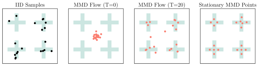
Figure 1: Quantisation of a mixture of $4$ distinct cross-shaped uniform distributions with (Left) $20$ i.i.d. samples and (Right) $20$ stationary MMD points computed via a discretised gradient flow, simulated for a sufficient length of time $T$ (also shown are the intermediate times $T=0$ and $T=20$). Stationary MMD points correspond in this case to a local minimum of the MMD, as there are $4$ samples in the first cross and $6$ samples in the second cross; these points can be explicitly computed. Minimum MMD points (not shown) would (presumably) assign $5$ points to each cross, but such points cannot be computed in general.

Our Contributions: In this paper, we address this question by studying the asymptotic cubature performance of stationary MMD points, defined as point sets $\{\bm{x}_{i}\}_{i=1}^{n}$ for which the associated empirical measure $\mu_{n}$ satisfies:

1. $\operatorname{MMD}(\mu,\mu_{n})\to 0$ as $n\to\infty$.  

2. The gradient of $\operatorname{MMD}(\mu,\mu_{n})$ with respect to $\{\bm{x}_{i}\}_{i=1}^{n}$ equals $\bm{0}$.

Although minimum MMD points also satisfy LABEL:as:convergence and LABEL:as:stationary, the class of stationary MMD points represents a strict relaxation: they can be obtained via gradient-based optimization simulated to a local minimum (see Figure˜1). Our first main result is that stationary MMD points achieve a faster-than-MMD cubature rate for a wide class of functions $f$ in $\mathcal{H}$ (˜3.4):

$$\left|\frac{1}{n}\sum_{i=1}^{n}f(\bm{x}_{i})-\int f\;\mathrm{d}\mu\right|=o\left(\operatorname{MMD}(\mu,\mu_{n})\right).$$ (3)

Comparing (3) and (2) shows that cubature using stationary MMD points converges faster than the worst-case scenario anticipated by the MMD. This is surprising, but not paradoxical, as the integrand $f$ in (3) is fixed, while $f_{n}=\frac{1}{n}\sum_{i=1}^{n}k(\bm{x}_{i},\cdot)-\int k(\bm{x},\cdot)\mathrm{d}\mu(\bm{x})$, the integrand that realises equality in (2), is dependent on the point set $\{\bm{x}_{i}\}_{i=1}^{n}$. Thus (3) can be interpreted as a novel form of super-convergence (see Schaback (2018) and ˜3.5). The intuition behind our proof of this result is that stationary MMD points achieve exact integration (i.e., zero cubature error) for a large linear subspace of $\mathcal{H}$, and this subspace expands as $n$ is increased.

Our second main result confirms that stationary MMD points can be obtained exactly through an interacting particle systems simulated until stationarity (˜4.2)—a property that does not hold for their minimum MMD points counterpart. The particle system considered is derived from MMD gradient flow (Arbel et al., 2019; Hertrich et al., 2024b; Duong et al., 2024), which formulates an optimization problem in the space of probability distributions over $\mathbb{R}^{d}$. To this end, we prove a novel non-asymptotic rate of convergence for the time-discretised, finite-particle MMD gradient flow (˜4.1). Our analysis incorporates the noise injection scheme proposed in Arbel et al. (2018) and builds upon recent advances in non-asymptotic finite-particle analysis of gradient flows (Banerjee et al., 2025), which may be of independent interest. Finally, the effectiveness of stationary MMD points for cubature is confirmed via an empirical assessment.

2 Related Work

Before we present our new results, we first review existing work on quantisation of probability measures $\mu$ related to MMD. Our focus is restricted to uniformly-weighted empirical measures $\mu_{n}$; a discussion of alternative methods and results, including those based on weighted empirical measures, is contained in Appendix˜A. Uniform weights are often preferred due to their simplicity, numerical stability, and robustness to violation of assumptions on the integrand.

Minimum MMD / Energy Points:

Similar to minimum MMD points, there is a rich literature studying point sets, called minimum energy points, that minimise an energy functional of the form $\frac{1}{n^{2}}\sum_{i,j=1}^{n}\rho(\bm{x}_{i},\bm{x}_{j})-\frac{2}{n}\sum_{i=1}^{n}\operatorname{\mathbb{E}}_{\bm{y}\sim\mu}[\rho(\bm{x}_{i},\bm{y})]$. For instance, minimum energy points were studied to construct well-separated nodes over a unit sphere with $\rho(\bm{x},\bm{x}^{\prime})=\|\bm{x}-\bm{x}^{\prime}\|^{-r}$ for $0<r<2$, where $\lVert\cdot\rVert$ denotes the Euclidean norm on $\mathbb{R}^{d}$ (Brauchart and Grabner, 2015; Marzo and Mas, 2021; Grabner, 2014). For $\rho(\bm{x},\bm{x}^{\prime})=-\|\bm{x}-\bm{x}^{\prime}\|$, it was proved in Mak and Joseph (2018) that the cubature error of minimum energy points is $\mathcal{O}(n^{-\frac{1}{2}}(\log n)^{-\frac{1}{2d}})$, calling them support points. This energy functional coincides (up to an additive constant) with the squared MMD in the special case where $\rho$ is a kernel. As with minimum MMD points, the algorithms proposed in Mak and Joseph (2018); Hertrich et al. (2024b) do not come with guarantees of finding minimum energy configurations in general. Our contribution addresses this by analysing the properties of stationary MMD points in Section˜3. Interestingly, Sloan and Womersley (2009) study the properties of stationary energy points over a unit sphere and prove that stationary energy points are indeed minimum energy points if they are sufficiently well-separated in the geodesic distance.

Quasi Monte Carlo:

Sophisticated quasi Monte Carlo (QMC) point sets have been developed for common distributions $\mu$, typically uniform distributions on a hypercube, $d$-sphere, or simple transformations thereof (Dick and Pillichshammer, 2010; Klebanov and Sullivan, 2023). Although QMC can exhibit a fast rate of convergence in cubature, and these points can be explicitly computed, it does not currently represent a solution for general targets $\mu$ on $\mathbb{R}^{d}$ (e.g $\mu$ in Figure˜1). The traditional discrepancy used in QMC is the star discrepancy, while much of the modern literature on QMC adopts the more general perspective of MMD (Hickernell, 1998).

Compression:

Kernel herding is a sequential algorithm that performs conditional gradient descent on the MMD (Chen et al., 2010). It requires solving non-convex optimization problems for the next point, which can be approximated by searching over a large candidate set $\{\bm{y}_{i}\}_{i=1}^{N}$, but little is known about its theoretical properties except for in finite-dimensional RKHSs (Bach et al., 2012; Santin et al., 2021). Greedy minimisation of MMD was proposed in Teymur et al. (2021), again selecting points from a large candidate set $\{\bm{y}_{i}\}_{i=1}^{N}$, with a slower-than-Monte Carlo rate for infinite-dimensional RKHSs. Kernel thinning is a compression algorithm that selects the top $n$ most representative points from a large dataset $\{\bm{y}_{i}\}_{i=1}^{N}$ also by minimizing the MMD (Dwivedi and Mackey, 2024). The main distinction between these algorithms and our stationary MMD points is that we do not constrain our points $\{\bm{x}_{i}\}_{i=1}^{n}$ to be a subset of a candidate set $\{\bm{y}_{i}\}_{i=1}^{N}$.

Gradient Flows:

Recently, a line of research on Wasserstein gradient flows frames the approximation of $\mu$ as optimization of a statistical divergence $\mathcal{D}(\cdot\|\mu)$ over a space of probability distributions. Concerning cubature, among the various choices for $\mathcal{D}$ a natural candidate is MMD due to the connection to cubature error in (2). The resulting MMD gradient flow was introduced in Arbel et al. (2019) and has been widely-used in generative modelling (Galashov et al., 2025; Hertrich et al., 2024b; Altekrüger et al., 2023; Hertrich et al., 2024a). It has also demonstrated strong empirical performance for cubature (Xu et al., 2022; Chen et al., 2021; Belhadji et al., 2025). Unfortunately, a formal theoretical study of the convergence of time-discretised finite-particle MMD gradient flow is missing in the literature—the primary challenge is that MMD is non-convex in the Wasserstein metric (Chen et al., 2024). Our second main theoretical contribution is a novel theoretical analysis that addresses this gap, in Section˜4, and which may be of independent interest. Related to this result, Boufadène and Vialard (2023) recently proved global convergence of MMD gradient flow for the Riesz kernel, under conditions that include boundedness of the logarithms of the candidate and target densities. However, as these results do not apply to the finite particle setting, or to targets supported on non-compact domains, they cannot be used in our context.

3 Cubature Properties of Stationary MMD Points

This section establishes our first main result; super-convergence of stationary MMD points. The analysis of algorithms for computing stationary MMD points is deferred to Section˜4.

3.1 Set-Up and Notation

Let $\mathcal{P}(\mathbb{R}^{d})$ denote the set of Borel probability distributions on $\mathbb{R}^{d}$. Throughout we let $\mu\in\mathcal{P}(\mathbb{R}^{d})$ denote the distribution of interest, and we let $\mathcal{X}=\mathrm{supp}(\mu)\subseteq\mathbb{R}^{d}$ denote its support, i.e. the set of all $\bm{x}$ such that $\mu(B_{r}(\bm{x}))>0$ for all $r>0$, where $B_{r}(\bm{x})$ is an open ball of radius $r$ centered at $\bm{x}\in\mathbb{R}^{d}$. Let $k\colon\mathbb{R}^{d}\times\mathbb{R}^{d}\to\mathbb{R}$ be a symmetric positive semi-definite kernel and $\mathcal{H}$ be its associated RKHS (Aronszajn, 1950), a Hilbert space of functions on $\mathbb{R}^{d}$ with inner product $\langle\cdot,\cdot\rangle_{\mathcal{H}}$ and norm $\|f\|_{\mathcal{H}}=\sqrt{\langle f,f\rangle_{\mathcal{H}}},$ containing $\mathrm{span}\{k(\bm{x},\cdot):x\in\mathbb{R}^{d}\}$ as a dense subset, and for which the reproducing property $f(\bm{x})=\langle f,k(\bm{x},\cdot)\rangle_{\mathcal{H}}$ holds for all $f\in\mathcal{H}$ and $\bm{x}\in\mathbb{R}^{d}$.

Given a function $f\colon\mathbb{R}^{d}\to\mathbb{R}$, let $\partial_{\ell}f(\bm{x})$ denote the partial derivative with respect to the $\ell$-th coordinate in $\bm{x}$ and denote $\nabla f(\bm{x})=[\partial_{1}f(\bm{x}),\ldots,\partial_{d}f(\bm{x})]^{\top}\in\mathbb{R}^{d}$. Let $\partial_{\ell}k(\bm{x},\bm{x}^{\prime})$ denote the partial derivative with respect to the $\ell$-th coordinate of $\bm{x}$ and let $\partial_{\ell}\partial_{\ell+d}k(\bm{x},\bm{x}^{\prime})$ denote the mixed partial derivative with respect to the $\ell$-th coordinate in $\bm{x}$ and the $\ell$-th coordinate in $\bm{x}^{\prime}$. Moreover, denote $\nabla_{1}k(\bm{x},\bm{x}^{\prime})=[\partial_{1}k(\bm{x},\bm{x}^{\prime}),\ldots,\partial_{d}k(\bm{x},\bm{x}^{\prime})]^{\top}\in\mathbb{R}^{d}$.

Throughout the paper, we make the following assumption on the kernel $k$:

Assumption 1 ($\mu$-integrability and differentiability).

Assume that $\sup_{\bm{x}\in\mathbb{R}^{d}}\int k(\bm{x},\bm{y})\;\mathrm{d}\mu(\bm{y})<\infty$ and $\sup_{\bm{x}\in\mathbb{R}^{d}}\int\partial_{\ell}k(\bm{x},\bm{y})\;\mathrm{d}\mu(\bm{y})<\infty$ for each $\ell\in\{1,\ldots,d\}$, and that $(\bm{x},\bm{y})\mapsto\partial_{\ell}\partial_{\ell+d}k(\bm{x},\bm{y})$ is continuous on $\mathbb{R}^{d}\times\mathbb{R}^{d}$.

This assumption is satisfied by popular kernels including Gaussian, Laplacian, Matérn, and inverse multiquadric kernels. It is also satisfied by linear kernel $k(\bm{x},\bm{y})=\bm{x}^{\top}\bm{y}$ when $\mu$ is a mean-zero distribution. The $\mu$-integrability of $k$ ensures that the integrals in (1) are well-defined (Smola et al., 2007). From Corollary 4.36 of Steinwart and Christmann (2008), for kernels that satisfy Assumption˜1, we know that $\partial_{\ell}k(\bm{x},\cdot)\in\mathcal{H}$ for any $\bm{x}\in\mathbb{R}^{d}$ and any $\ell\in\{1,\ldots,d\}$.

3.2 First Main Result: Super-Convergence of the Cubature Error

The key to our first main result, on super-convergence of the cubature error, is an observation that the stationary MMD points $\{\bm{x}_{i}\}_{i=1}^{n}$ exactly integrate a linear subspace:

$$\mathcal{G}_{\mathcal{X}_{n}}\coloneqq\mathrm{span}\{\partial_{\ell}k(\bm{x},\cdot):\;\bm{x}\in\mathcal{X}_{n},\;1\leq\ell\leq d\}\subset\mathcal{H},\quad\mathcal{X}_{n}=\{\bm{x}_{i}\}_{i=1}^{n}\subset\mathbb{R}^{d}.$$ (4)

as shown in the following proposition:

Proposition 3.1 (Cubature exactness).

Suppose the kernel $k$ satisfies Assumption˜1. Then cubature using $\{\bm{x}_{i}\}_{i=1}^{n}$ is exact on $\mathcal{F}_{n}\coloneqq\mathrm{span}(\{1\}\cup\mathcal{G}_{\mathcal{X}_{n}})$. That is, $\frac{1}{n}\sum_{i=1}^{n}f(\bm{x}_{i})=\int f\mathrm{d}\mu$ for all $f\in\mathcal{F}_{n}$.

Proof of ˜3.1 Since the cubature weights sum to 1, $\mu_{n}$ is exact on the constant functions, $\mathrm{span}(\{1\})$. We are thus left to check the exactness on $\mathcal{G}_{\mathcal{X}_{n}}$. The LABEL:as:stationary condition reads, for each $i\in\{1,\dots,n\}$,

$$\nabla_{\bm{x}_{i}}\operatorname{MMD}^{2}\Big{(}\mu,\frac{1}{n}\sum_{j=1}^{n}\delta_{\bm{x}_{j}}\Big{)}=\bm{0}\iff\frac{1}{n}\sum_{j=1}^{n}\nabla_{1}k(\bm{x}_{i},\bm{x}_{j})-\int\nabla_{1}k(\bm{x}_{i},\bm{y})\mathrm{d}\mu(\bm{y})=\bm{0},$$ (5)

where we have interchanged $\mu$-integral and derivative (justified under Assumption˜1; see Lemma˜B.1). This final equation shows that the cubature rule $\mu_{n}$ is exact on $\bm{x}\mapsto\partial_{\ell}k(\bm{x}_{i},\bm{x})$ for each $\ell\in\{1,\ldots,d\}$ and $i\in\{1,\dots,n\}$, completing the argument. ∎

Remark 3.2 (Example of $\mathcal{G}_{\mathcal{X}_{n}}$).

To gain more insight into the space $\mathcal{G}_{\mathcal{X}_{n}}$, consider a polynomial kernel $k(\bm{x},\bm{y})=(\bm{x}^{\top}\bm{y}+1)^{r}$, where $r\in\mathbb{N}$. In this setting, let $\varphi_{r}\colon\mathbb{R}^{d}\to\mathbb{R}^{m}$ denote the feature map consisting of all monomials of total degree $\leq r$ (excluding constant functions), where $m=\binom{d+r}{r}-1$. If the matrix $\Phi_{r}\coloneqq[\varphi_{r}(\bm{x}_{1}),\ldots,\varphi_{r}(\bm{x}_{n})]\in\mathbb{R}^{m\times n}$ has rank $m$, then $\mathcal{G}_{\mathcal{X}_{n}}$ coincides with the space of all polynomial functions of degree $\leq r$ (excluding constant functions), meaning the cubature rule is polynomially exact. This can be contrasted with Karvonen et al. (2018), which relies on non-uniform weights to minimise MMD (for a fixed point set) subject to a polynomial exactness constraint.

Given an integrand $f$, we can consider a decomposition $f=f_{n}+(f-f_{n})$ where $f_{n}\in\mathcal{F}_{n}$ is exactly integrated by ˜3.1. The cubature error therefore depends only on the difficulty of numerically integrating the remainder term $f-f_{n}$. This observation motivates us to investigate the approximation capacity of $\mathcal{F}_{n}$ with respect to the whole RKHS $\mathcal{H}$. To this end, we make the following assumptions:

Assumption 2 (Support connectedness).

For any two points $\bm{x},\bm{y}\in\mathcal{X}$, there exists a piecewise continuously differentiable curve $\gamma\colon[0,1]\to\mathcal{X}$ with $\gamma(0)=\bm{x}$ and $\gamma(1)=\bm{y}$.

This assumption holds if $\mathcal{X}$ is the closure of an open connected set or an embedded $C^{1}$ manifold, which includes common sets such as $\mathbb{R}^{d}$, spheres or spherical surfaces as examples. This assumption can be relaxed to $\mathcal{X}$ being the finite union of sets satisfying Assumption˜2 (as illustrated in Figure˜1) if $\mathcal{H}$ does not contain non-zero constant functions on the subsets, as is the case for Gaussian RKHSs and subsets with non-empty interiors (Steinwart and Christmann, 2008, Corollary 4.44).

Assumption 3 ($C_{0}$-universality).

The kernel $k$ is $C_{0}$-universal; i.e., the associated RKHS $\mathcal{H}$ has a subset that is dense in $C_{0}(\mathbb{R}^{d})$, the space of continuous functions $f:\mathbb{R}^{d}\to\mathbb{R}$ that vanish at infinity, with respect to the norm $\|f\|_{\infty}=\sup_{\bm{x}\in\mathbb{R}^{d}}|f(\bm{x})|$.

The reader is referred to Carmeli et al. (2010); Sriperumbudur et al. (2011) for a detailed discussion of $C_{0}$-universal kernels. Assumptions˜1 and 3 are satisfied by Gaussian, Laplacian, Matérn, and inverse multiquadric kernels.

˜3.3 below formalizes the approximation capacity of $\mathcal{F}_{n}$. To state this result, we let $\mathcal{H}_{\mathcal{X}}$, denote the closure of $\mathrm{span}\{k(\bm{x},\cdot):\bm{x}\in\mathcal{X}\}$ in $\mathcal{H}$.

Proposition 3.3 (Asymptotic approximation capacity of $\mathcal{F}_{n}$).

Suppose $\mathcal{X}$ satisfies Assumption˜2 and $k$ satisfies Assumptions˜1 and 3. Let $f=c+h$ with $c\in\mathbb{R}$, $h\in\mathcal{H}_{\mathcal{X}}$, and consider the semi-norm

$$|f|_{n}\coloneqq\inf\{\|r_{n}\|_{\mathcal{H}}\;:\;f=f_{n}+r_{n},\;f_{n}\in\mathcal{F}_{n},\;r_{n}\in\mathcal{H}\}.$$ (6)

If $h$ is non-constant on $\mathcal{X}$, then $\lim_{n\to\infty}|f|_{n}=0$.

Proof of ˜3.3.

For any $\varepsilon>0$, we show $|f|_{n}<\varepsilon$ for sufficiently large $n\in\mathbb{N}$. The key observation is that we can approximate $h$ using an element of $\mathcal{G}_{\mathcal{X}}\coloneqq\mathrm{span}\{\partial_{\ell}k(\bm{x},\cdot):\bm{x}\in\mathcal{X},1\leq\ell\leq d\}$, which can be further approximated by an element of $\mathcal{G}_{\mathcal{X}_{n}}$. The denseness of $\mathcal{G}_{\mathcal{X}_{n}}$ follows from the denseness of stationary MMD points in $\mathcal{X}$, due to its LABEL:as:convergence property. These claims are proved in Lemmas˜B.5 and B.6 (see Sections˜B.3 and B.2). Formally, by Lemma˜B.5, there exists $g_{\varepsilon}\in\mathcal{G}_{\mathcal{X}}$ satisfying $\|h-g_{\varepsilon}\|_{\mathcal{H}}<\varepsilon/2$. Also, Lemma˜B.6 states that for sufficiently large $n\in\mathbb{N}$, we may take $g_{n,\varepsilon}\in\mathcal{G}_{\mathcal{X}_{n}}$ such that $\|g_{\varepsilon}-g_{n,\varepsilon}\|_{\mathcal{H}}<\varepsilon/2$. Since $f=c+g_{n,\varepsilon}+h-g_{\varepsilon}+g_{\varepsilon}-g_{n,\varepsilon}$, the definition of $|f|_{n}$ in (6) implies $|f|_{n}\leq\|h-g_{\varepsilon}\|_{\mathcal{H}}+\|g_{\varepsilon}-g_{n,\varepsilon}\|_{\mathcal{H}}<\varepsilon$. ∎

The subset $\mathcal{H}_{\mathcal{X}}\subset\mathcal{H}$ consists of functions that do not vanish on $\mathcal{X}$ (see ˜B.3). ˜3.3 therefore states that $\mathcal{G}_{\mathcal{X}_{n}}$ can approximate functions in $\mathcal{H}$ with non-trivial $\mu$-integrals increasingly well as the sample size $n$ is increased. Now we are able to state our main theorem, which shows that the cubature error of stationary MMD points vanishes faster than MMD:

Theorem 3.4 (Super-convergence of stationary MMD points).

Suppose the kernel $k$ satisfies Assumption˜1. For each $n\in\mathbb{N}$, the cubature error of a stationary MMD point set $\{\bm{x}_{i}\}_{i=1}^{n}$ for an integrand $f\in\mathrm{span}(\{1\}\cup\mathcal{H})$ satisfies

$$\left|\frac{1}{n}\sum_{i=1}^{n}f(\bm{x}_{i})-\int f\mathrm{d}{\mu}\right|\leq|f|_{n}\cdot\mathrm{MMD}\left(\mu,\mu_{n}\right).$$ (7)

Furthermore, suppose $\mathcal{X}$ satisfies Assumption˜2 and $k$ satisfies Assumption˜3. Let $f=c+h$ with $c\in\mathbb{R}$ and $h\in\mathcal{H}_{\mathcal{X}}$ non-constant on $\mathcal{X}$. Then $|f|_{n}\to 0$ as $n\to\infty$, so the cubature rule achieves a super MMD error rate $o\left(\operatorname{MMD}(\mu,\mu_{n})\right)$.

Proof of ˜3.4.

The proof exploits the control variate trick of Bakhvalov (2015). The integrand $f$ can be written as $f=f_{n}+r_{n}$ with $f_{n}\in\mathcal{F}_{n}$, whence

$$\left|\frac{1}{n}\sum_{i=1}^{n}f(\bm{x}_{i})-\int f\;\mathrm{d}\mu\right|=\left|\frac{1}{n}\sum_{i=1}^{n}r_{n}(\bm{x}_{i})-\int r_{n}\;\mathrm{d}\mu\right|\leq\|r_{n}\|_{\mathcal{H}}\cdot\mathrm{MMD}\left(\mu,\mu_{n}\right),$$

where the equality follows since $f_{n}\in\mathcal{F}_{n}$ is exactly integrated (see ˜3.1) and the inequality is Cauchy–Schwarz. Taking the infimum over all possible choices of $r_{n}$ in the decomposition of $f$ yields $|\frac{1}{n}\sum_{i=1}^{n}f(\bm{x}_{i})-\int f\;\mathrm{d}\mu|\leq|f|_{n}\cdot\mathrm{MMD}(\mu,\mu_{n})$. ˜3.3 proves that $\lim_{n\to\infty}|f|_{n}=0$ when $f=c+h$ with $c\in\mathbb{R}$ and $h\in\mathcal{H}_{\mathcal{X}}$ non-constant on $\mathcal{X}$, completing the argument. ∎

Remark 3.5 (Super-convergence).

In approximation theory, the term super-convergence usually refers to how a worst-case error error bound, such as (2), can be bypassed if additional regularity can be exploited. In kernel settings, several rate doubling results exist for $f$ with, roughly speaking, twice the smoothness of the RKHS, in that $f$ is in the range of the integral operator associated to the kernel (Schaback, 1999, 2018; Sloan and Kaarnioja, 2025). A result analogous to ˜3.4 can be trivially deduced for optimal non-uniform weights (see Appendix˜A and (Fasshauer, 2011; Karvonen, 2022)); one interpretation of ˜3.4 is that non-uniform weights are not required to attain super-convergence in the cubature context.

4 Computing Stationary MMD Points

This section explains how stationary MMD points can be practically computed. To this end we consider an MMD gradient flow, which starts by initialising particles $\smash{\{\bm{x}_{i}^{(1)}\}_{i=1}^{n}\subset\mathbb{R}^{d}}$ and then, for kernels that satisfy Assumption˜1, these particles are updated via gradient descent on the (squared) MMD:

$$\bm{x}_{i}^{(t+1)}=\bm{x}_{i}^{(t)}-\gamma\left\{\mathbb{E}_{\bm{Y}\sim\mu}[\nabla_{1}k(\bm{x}_{i}^{(t)},\bm{Y})]-\frac{1}{n}\sum_{j=1}^{n}\nabla_{1}k(\bm{x}_{i}^{(t)},\bm{x}_{j}^{(t)})\right\},\quad t\in\{1,\ldots,T\},$$ (8)

where $\gamma>0$ is a step size to be specified. The update (8) can equivalently be viewed as a discretised Wasserstein gradient flow on the MMD (Arbel et al., 2019, Equation 21), and thus it decreases MMD in the steepest direction in terms of both the Euclidean and Wasserstein geometry: $\mathrm{MMD}(\mu,\hat{\nu}^{(t+1)}_{n})\leq\mathrm{MMD}(\mu,\hat{\nu}^{(t)}_{n})$ where $\hat{\nu}^{(t)}_{n}$ is the empirical measure of the particles at time $t$, provided the step size $\gamma$ is small enough (see Proposition 4 of Arbel et al. (2019) and our Lemma˜B.7). Naturally, if we simulate (8) for long enough the LABEL:as:stationary property will be satisfied; this is verified numerically in Section˜5.

Unfortunately, even though (8) is guaranteed to decrease MMD at each step, the MMD gradient flow $(\hat{\nu}^{(t)}_{n})_{t=1}^{\infty}$ might still fail to converge to the target distribution $\mu$ even with infinite time steps and infinite number of particles, which violates the first LABEL:as:convergence property of the stationary MMD points. Indeed, this is a well-known challenge for MMD gradient flows (8) due to lack of convexity of MMD with respect to the Wasserstein-2 metric (Chen et al., 2024). As a result, there exists a gap between theoretical results and practical algorithms that minimise the MMD (Xu et al., 2022; Mak and Joseph, 2018; Chen et al., 2021).

To improve convergence of MMD gradient flow, we follow Arbel et al. (2019) and inject noise into (8). Specifically, with $(\bm{u}_{i}^{(t)})_{i=1}^{n}\sim\mathcal{N}(0,\mathrm{I}_{d})$ and $\beta_{t}>0$ for $t\in\mathbb{N}$,

$$\bm{x}_{i}^{(t+1)}=\bm{x}_{i}^{(t)}-\gamma\left\{\mathbb{E}_{\bm{Y}\sim\mu}[\nabla_{1}k(\bm{x}_{i}^{(t)}+\beta_{t}\bm{u}_{i}^{(t)},\bm{Y})]-\frac{1}{n}\sum_{j=1}^{n}\nabla_{1}k(\bm{x}_{i}^{(t)}+\beta_{t}\bm{u}_{i}^{(t)},\bm{x}_{j}^{(t)})\right\}.$$ (9)

We call the above update scheme (9) noisy MMD particle descent with noise scale $\beta_{t}$, and we will show in Section˜4.1 that it indeed converges to stationary MMD points as desired. It is a key point of distinction relative to minimum MMD points, which cannot be computed in general.

To implement (9) the expectation $\operatorname{\mathbb{E}}_{\bm{Y}\sim\mu}[\nabla_{1}k(\cdot,\bm{Y})]$ is required. For certain kernels $k$ and targets $\mu$ this can be exactly computed; see, for example, Briol et al. (2019) for a comprehensive list of closed-form kernel mean embeddings which can then be differentiated, or Chen et al. (2025) for the use of change-of-variable techniques to facilitate such computations. When $\mu$ is only known up to a normalisation constant, Stein reproducing kernels provide a viable alternative (Oates et al., 2017). Moreover, when $\mu$ corresponds to an empirical distribution supported on a dataset, $\operatorname{\mathbb{E}}_{\bm{Y}\sim\mu}[\nabla_{1}k(\cdot,\bm{Y})]$ can be computed trivially, since the expectation reduces to an empirical average over the dataset.

4.1 Second Main Result: Finite Particle Error Bounds for MMD Gradient Flow

A novel convergence analysis of noisy MMD particle descent (8) is the second main contribution of this paper. In particular, we show that (8) indeed finds the stationary MMD points under the following additional assumptions:

Assumption 4 (Kernel regularity).

The maps $\bm{x}\mapsto k(\bm{x},\bm{x})$, $\bm{x}\mapsto\partial_{\ell}\partial_{\ell+d}k(\bm{x},\bm{x})$, and $\bm{x}\mapsto\partial_{\ell}\partial_{r}\partial_{r+d}\partial_{\ell+d}k(\bm{x},\bm{x})$ are continuous and bounded, uniformly over $r,\ell\in\{1,\ldots,d\}$, by a positive constant $\kappa$.

Assumption˜4 is a standard assumption in the literature on Wasserstein gradient flows with smooth kernels (Glaser et al., 2021; Arbel et al., 2019; He et al., 2024; Korba et al., 2020). Many kernels satisfy Assumptions˜1, 3 and 4, including the Gaussian kernel, Matérn kernel of order $\zeta$ with $\zeta+d/2\geq 2$, and the inverse multiquadratic kernel.

Assumption 5 (Noise injection level).

Define $\Phi(\bm{z},\bm{w})=\operatorname{\mathbb{E}}_{\bm{Y}\sim\mu}[\nabla_{1}k(\bm{z},\bm{Y})]-\nabla_{1}k(\bm{z},\bm{w})$. For each $t\in\mathbb{N}^{+}$, the noise injection level $\beta_{t}\in(0,1)$ satisfies, with $\underline{\bm{u}}^{(t)}\coloneqq(\bm{u}_{i}^{(t)})_{i=1}^{n}\overset{\mathrm{i.i.d.}}{\sim}\mathcal{N}(0,\mathrm{I}_{d})$,

$$\frac{1}{n}\sum\limits_{i=1}^{n}\operatorname{\mathbb{E}}_{\underline{\bm{u}}^{(t)}}\left[\left\|\frac{1}{n}\sum_{j=1}^{n}\Phi(\bm{x}_{i}^{(t)}+\beta_{t}\bm{u}_{i}^{(t)},\bm{x}_{j}^{(t)})\right\|^{2}\right]\geq 4\beta_{t}^{2}d^{2}\kappa^{2}\operatorname{MMD}^{2}\left(\frac{1}{n}\sum_{i=1}^{n}\delta_{\bm{x}_{i}^{(t)}},\mu\right).$$ (10)

Assumption˜5 states that with appropriate control of noise injection level $\beta_{t}$, the noisy MMD particle descent satisfies a gradient dominance condition in expectation (also known as the Polyak–Lojasiewicz inequality), a weaker condition than convexity to ensure fast global convergence (Boyd and Vandenberghe, 2004). A posteriori verification of Assumption˜5 is possible by drawing many realisations of the injected noise and taking an empirical average as an estimate of the expectation of the left side in (10). Since $\Phi$ is bounded from Assumption˜4, this empirical estimate is expected to concentrate fast to its expectation. Similar assumptions have been used in the convergence analysis of kernel-based gradient flows; see Proposition 8 of Arbel et al. (2019) and Proposition 5 of Glaser et al. (2021). However, their assumptions on $\beta_{t}$ involve also expectations with respect to $\{\bm{x}_{i}^{(t)}\}_{i=1}^{n}$ on both sides of (10), which means their assumptions need to be checked for any possible trajectory; in contrast, our assumption only needs to be checked for the current trajectory.

Theorem 4.1.

Suppose the kernel $k$ satisfies Assumptions˜1 and 4. Given initial particles $\{\bm{x}_{i}^{(1)}\}_{i=1}^{n}$, suppose the noisy MMD particle descent defined in (9) satisfies Assumption˜5. Suppose step size $\gamma$ satisfies $256\gamma^{2}d^{2}\kappa^{2}\leq 1$. Then for any $T\in\mathbb{N}^{+}$, for any $\delta>0$, with probability at least $1-\exp(-\delta)$,

$$\operatorname{MMD}\left(\frac{1}{n}\sum_{i=1}^{n}\delta_{\bm{x}_{i}^{(T)}},\mu\right)\leq{} \underbrace{\exp\left(-\sum\limits_{t=1}^{T-1}\frac{1}{2}\gamma\beta_{t}^{2}\kappa d^{2}\right)\operatorname{MMD}\left(\frac{1}{n}\sum\limits_{i=1}^{n}\delta_{\bm{x}_{i}^{(1)}},\mu\right)}_{\text{Optimisation error}}$$ (11)

$$+\underbrace{\frac{\delta+\log T}{\sqrt{n}}\cdot\left(\sum\limits_{t=1}^{T-1}C\sqrt{\kappa}(\beta_{t}\vee n^{-\frac{1}{2}})\sqrt{d}\cdot\exp\left(-\sum\limits_{s=t+1}^{T-1}\frac{1}{2}\gamma\beta_{s}^{2}\kappa d^{2}\right)\right)}_{\text{Estimation error}}.$$

Here, $a\vee b=\max\{a,b\}$ and $C$ is a positive universal constant independent of $n,(\beta_{t})_{t=1}^{T}$, and $T$.

The proof ˜4.1 can be found in Section˜B.4. The right-hand side of (11) consists of two terms: an optimisation error and a finite-sample estimation error. The optimisation error captures the decay of the MMD from its initial value under the dynamics of noisy MMD particle descent. Its exponential decay rate is a direct consequence of the gradient dominance condition from Assumption˜5, and this term vanishes when $\sum_{t=1}^{T-1}\beta_{t}^{2}\to\infty$ as $T\to\infty$, recovering the convergence result in Proposition 8 of Arbel et al. (2019). The latter estimation error quantifies the statistical error incurred from using $n$ particles. The $1/\sqrt{n}$ scaling factor arises from a standard concentration inequality, as established in Lemma˜B.8. We highlight a trade-off between the optimisation and estimation errors: increasing the noise level $\beta_{t}$ accelerates the convergence (reducing optimisation error) but simultaneously increases the variance of the updates, leading to larger estimation error.

The exact non-asymptotic rate of convergence of the noisy MMD particle descent largely depends on the noise injection scheme $\beta_{t}$. ˜4.2, the proof of which can be found in Section˜B.4, provides further insight into this rate:

Corollary 4.2.

In the setting of ˜4.1, suppose that $\beta_{t}\propto t^{-\alpha}$ for $0\leq\alpha<1/2$ and that Assumption˜5 holds. Define the constant $C^{\prime}=0.5\gamma\kappa^{2}d^{2}$. Then, for any $T\leq n^{\frac{1}{2\alpha}}$,

$$\operatorname{MMD}(\hat{\nu}^{(T)}_{n},\mu)=\mathcal{O}_{P}\left(\exp\left(-C^{\prime}T^{1-2\alpha}\right)+n^{-\frac{1}{2}}(\log T)^{2}T^{\alpha}\right),\qquad\hat{\nu}^{(T)}_{n}=\frac{1}{n}\sum_{i=1}^{n}\delta_{\bm{x}_{i}^{(T)}}.$$ (12)

By choosing $T=\mathcal{O}((\log n)^{\frac{1}{1-2\alpha}})$, we obtain the convergence rate $\operatorname{MMD}(\hat{\nu}^{(T)}_{n},\mu)=\mathcal{O}_{P}(n^{-\frac{1}{2}})$ up to some logarithm factors, which implies that the particles $\{\bm{x}_{i}^{(T)}\}_{i=1}^{n}$ satisfy the LABEL:as:convergence property in the $n,T\to\infty$ limit. Furthermore, since $\lim_{t\to\infty}\beta_{t}=0$, the particles $\{\bm{x}_{i}^{(T)}\}_{i=1}^{n}$ obtained from the noisy MMD particle descent (9) also satisfy the LABEL:as:stationary property in the same limit. Therefore, ˜4.2 establishes that noisy MMD particle descent scheme in (9) can indeed compute stationary MMD points, as desired.

The computational cost of stationary MMD points simulated via noisy MMD particle descent is $\mathcal{O}(n^{2}T)$. Following the argument above, it suffices to take $T=\mathcal{O}((\log n)^{\frac{1}{1-2\alpha}})$ so the overall computational cost is $\mathcal{O}(n^{2})$ up to logarithm factors. Compared to QMC which is computationally cheaper, stationary MMD points offer greater generality, as they can be applied to any target distribution $\mu$ supported on any domain $\mathcal{X}$ that satisfies Assumption˜2. Compared to existing approaches based on minimising the MMD or energy functionals—which share the same computational complexity as our stationary MMD points and often claim fast convergence rates (Mak and Joseph, 2018; Xu et al., 2022)—we highlight a gap between these theoretical guarantees and the practical issue of their proposed algorithms being trapped in local minima or stationary points. Our stationary MMD points are designed to bridge this gap. One can deduce $o_{P}(n^{-1/2})$ convergence rates of cubature error by combining the MMD convergence rate from ˜4.2 and the super-convergence result proved in ˜3.4.

Remark 4.3 (Comparison with existing convergence results in Arbel et al. (2019)).

Our ˜4.1 provides the first convergence result for time-discretised finite-particle MMD gradient flow with smooth kernels. In contrast, Proposition 8 of Arbel et al. (2019) proves convergence for the time-discretized population MMD flow, while Theorem 9 of Arbel et al. (2019) proves convergence of the time-discretized finite-particle MMD flow to its population limit, under the condition $T\geq n\gamma$. However, gluing these existing results together gives $\operatorname{MMD}(\hat{\nu}^{(T)}_{n},\mu)=\mathcal{O}(\exp(-C^{\prime}T^{1-2\alpha})+n^{-0.5}\exp(C^{\prime\prime}T))$ which does not converge when $T\geq n\gamma$.

Remark 4.4 (Finite particle error bound).

Establishing convergence for finite-particle implementations of Wasserstein gradient flows is a challenging task. A common approach involves controlling the propagation of chaos at each iteration, which typically results in an upper-bound that grows exponentially with $T$; see for example Arbel et al. (2019, Theorem 9), Shi and Mackey (2024, Theorem 3), and Chen et al. (2024, Proposition 10.1). In contrast, in ˜4.2, our upper-bound is polynomial and even logarithmic in $T$ when $\alpha=0$. The key insight of our ˜4.1 and ˜4.2, borrowed from Banerjee et al. (2025), is to work directly with the joint distribution of the particles and track the evolution of the squared MMD.

5 Experiments

This section numerically studies the cubature properties of stationary MMD points computed via noisy MMD particle descent scheme in (9). The python code to reproduce all the following experiments can be found at https://github.com/hudsonchen/MMDF_cubature.

5.1 Mixture of Gaussians

First we consider a synthetic experiment with the target distribution $\mu=\frac{1}{10}\sum_{m=1}^{10}\mathcal{N}(\bm{\mu}_{m},\bm{\Sigma}_{m})$, a mixture of 10 two-dimensional ($d=2$) Gaussian distributions following the set-up in Chen et al. (2010); Huszár and Duvenaud (2012). This simple multimodal setting evaluates the ability of sampling methods to capture all modes of a distribution—something i.i.d. samples often fail to achieve, as they tend to assign an imbalanced number of samples across the mixture components. Our stationary MMD points are simulated with noisy MMD particle descent in (9) until stationarity ($T=10,000$). We used a step size $\gamma=1.0$ and noise injection level $\beta_{t}=t^{-0.5}$ such that Assumption˜5 is empirically satisfied (see Figure˜4). All particles were initialised at $\bm{0}$ and a Gaussian kernel $k(\bm{x},\bm{y})=\exp(-0.5\|\bm{x}-\bm{y}\|^{2})$ was used. The Gaussian kernel satisfies all Assumptions˜1, 4 and 3 required for the theoretical cubature rate of stationary MMD points to hold.

Stationarity:

First, we verify that stationary MMD points indeed satisfy the exact cubature property for integrands in $\mathcal{F}_{n}$. To this end, we consider a function $f(\bm{x})=\sum_{j=1}^{n}\sum_{\ell=1}^{d}\partial_{\ell}k(\bm{x}_{j},\bm{x})$. This integrand has a $\mu$-integral that can be computed analytically; see Appendix˜C for the derivations.

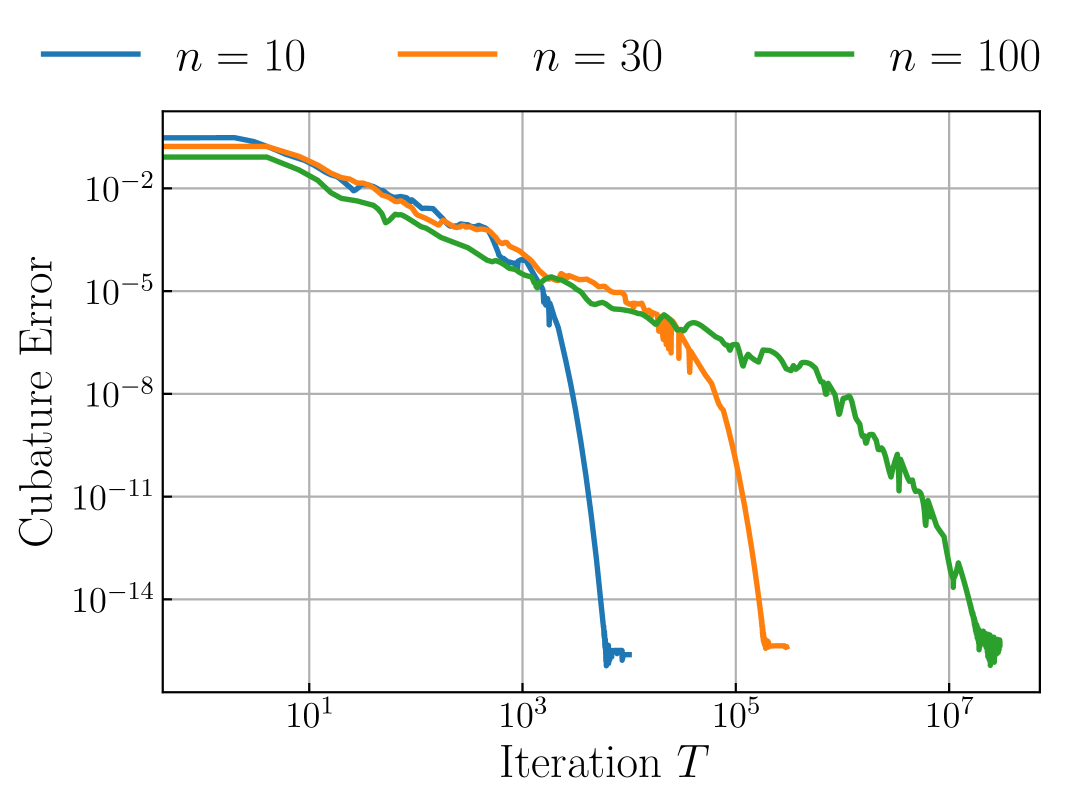
Figure 2: Exact cubature of a function in $\mathcal{F}_{n}$ with stationary MMD points computed by MMD gradient flow, verifying ˜3.1. The convergence plateaus at around $10^{-15}$ due to numerical precision.

We see in Figure˜2 that cubature error indeed vanishes when the noisy particle MMD descent scheme in (9) is simulated until stationarity. This empirically confirms the claim in ˜3.1. Although the noisy MMD particle descent scheme requires many iterations to reach convergence, we observe—consistent with ˜4.2—that it takes fewer iterations to have good cubature performance, as we demonstrate in the following results.

Cubature Benchmark:

Next, we consider cubature of the functions $f_{1}(\bm{x})=\exp(-0.5\|\bm{x}\|^{2})$ and $f_{2}(\bm{x})=\|\bm{x}\|^{2}$ against the distribution $\mu$. In this simple setting we have closed form expression for both integrals, which allows benchmarking against an array of baseline methods: $\mathrm{IID}$ represents identical independent samples, $\mathrm{QMC}$ represents quasi Monte Carlo samples, $\mathrm{KT}$ represents kernel thinning (Dwivedi and Mackey, 2024), $\mathrm{KH}$ represents kernel herding (Chen et al., 2010), and $\mathrm{SP}$ represents support points (Mak and Joseph, 2018). Note that we do not run KT for more than $512$ points because KT is computationally expensive, even with the latest speed-up in Shetty et al. (2022). Implementation details of all baselines can be found in Appendix˜C. In Top left and Top middle of Figure˜3, we observe that stationary MMD points consistently outperform all baselines in terms of cubature error for $f_{1}$, while achieving comparable performance to support points—and outperforming the remaining baselines—for $f_{2}$. This behavior is expected: $f_{1}\in\mathcal{H}$ so stationary MMD points are particularly well-suited for accurate integration; in contrast, $f_{2}\notin\mathcal{H}$ which explains the drop in relative performance. The strong performance of support points for $f_{2}$ can be attributed to the fact that support points minimise the energy distance with $\rho(\bm{x},\bm{y})=-\|\bm{x}-\bm{y}\|$ (Sejdinovic et al., 2013), which is analogous to MMD with an unbounded kernel, and hence support points may be more suitable for an unbounded integrand. Finally, we obtain the empirical rate by linear regression in log-log space. The cubature error with $f_{1}\in\mathcal{H}$ exhibits a rate of $-1.39$, while the MMD error decays at a rate of $-1.35$, which confirms the super-convergence predicted by ˜3.4.

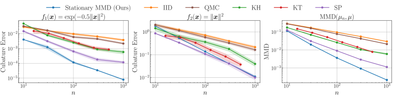
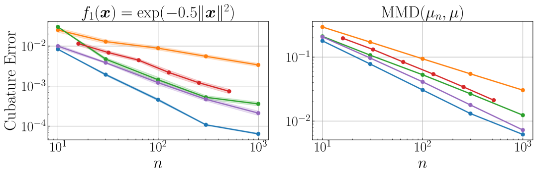
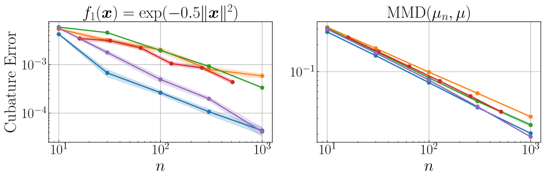
Figure 3: Comparison of stationary MMD points with baseline methods. Top row: mixture of Gaussians. Bottom left: House8L dataset. Bottom right: Elevators dataset. All results are averaged over 20 independent runs with different random seeds; shaded regions indicate 25%–75% quantiles.

5.2 OpenML Datasets

For our final experiment we considered the House8L ($d=8$) and Elevators ($d=18$) data from OpenML (Vanschoren et al., 2014), where the target $\mu$ is the empirical measure of the dataset. In this context, approximating $\mu$ by a discrete measure is commonly referred to as coreset selection (Bachem et al., 2017). Unlike standard coreset methods, our stationary MMD point set—obtained by noisy MMD particle descent simulated for $T=10,000$ iterations—does not consist of a subset of the original dataset. Although the support of $\mu$ does not meet Assumption˜2, our proposed algorithm can still be applied, and it is of interest to evaluate its empirical performance in such settings. We used a Gaussian kernel $k(\bm{x},\bm{y})=\exp(-0.5\|\bm{x}-\bm{y}\|^{2})$ and a fixed step size, $\gamma=1.0$ for House8L and $\gamma=0.3$ for Elevators. The noise injection level $\beta_{t}=t^{-0.5}$ empirically satisfied Assumption˜5 (see Figure˜4 in Appendix˜C). All particles were initialised at $\bm{0}$, reflecting the fact that the datasets are normalised. In Bottom of Figure˜3 we observe that stationary MMD points consistently outperform all baselines in terms of cubature error for $f_{1}$ and MMD. The improvement of stationary MMD points and all baselines are greater in House8L than Elevators, which we attribute to the lower dimensionality. To investigate the robustness of these results, Figure˜5 in Appendix˜C presents an ablation study comparing the performance of cubature methods based instead on the Matérn-$\frac{3}{2}$ kernel. For stationary MMD points, we observed that the Matérn-$\frac{3}{2}$ outperforms the Gaussian kernel on the House8L dataset. A variety of practical tools exist for kernel choice, but a comprehensive analysis of the interaction of these tools with the performance of stationary MMD points is beyond the scope of this work.

6 Discussion

This paper resolves an important open issue in discrete approximation of probability distributions; how to reconcile the theoretical performance of minimum MMD points with the reality that only stationary MMD points can be computed. Our analysis revealed the surprising result that the cubature error using stationary MMD points vanishes faster than the MMD – so-called super-convergence – providing for the first time an explanation of the strong empirical performance that had been previously observed. In addition, we have substantially strengthened the convergence analysis for noisy MMD particle descent, proving that stationary MMD points can be computed.

Limitations and Future Work:

Our algorithm requires access to a specific expectation $\operatorname{\mathbb{E}}_{\bm{Y}\sim\mu}[\nabla_{1}k(\cdot,\bm{Y})]$. Outside the setting where closed form expressions are available, numerical approximation can be used, but additional analysis to account for numerical error would be needed. A strength of our analysis is that the support $\mathcal{X}$ is general; in particular $\mu$ can be supported on a sufficiently smooth connected manifold embedded in $\mathbb{R}^{d}$, and mild extensions of this setting such as the four crosses example in Figure˜1. However, our results do not hold for general manifolds (i.e., ones that cannot be embedded into $\mathbb{R}^{d}$), and an intrinsic formulation on general manifolds is left as future work.

The idea of finding a subspace on which the cubature rule is exact is classical, underpinning Gaussian cubatures, and was considered also in Liu and Wang (2018) to analyze the cubature properties of stationary points in Stein variational gradient descent (Liu and Wang, 2016); it remains an interesting open question as to whether a super-convergence result can be established in that context.

Acknowledgments

ZC was supported by the Engineering and Physical Sciences Research Counci (EPSRC) HK and CJO were supported by EP/W019590/1. CJO was supported by a Philip Leverhulme Prize PLP-2023-004. FXB was supported by EPSRC EP/Y022300/1. TK was supported by the Research Council of Finland grant 359183 (Flagship of Advanced Mathematics for Sensing, Imaging and Modelling). The authors thank Matthew Fisher for his helpful comment on the support assumption.

Appendices

Appendix˜A describe further related work, including methods that employ non-uniform cubature weights and foundational results on approximation complexity for numerical integration. The proofs for all theoretical results presented in the main text are contained in Appendix˜B. Finally, additional details required to reproduce our experiments are contained in Appendix˜C.

Appendix A Further Related Work

This appendix briefly summarises several strands of related work, mainly focusing on methods that employ non-uniform weights; an important distinction from the main text.

Kernel Cubature: There is a rich line of research in the machine learning literature on cubature rules based on integrating a minimal norm interpolant. Indeed, if we let $f_{n}$ denote the element of $\mathcal{H}$ that interpolates $f$ at each element of $\{\bm{x}_{i}\}_{i=1}^{n}$ and for which $\|f_{n}\|_{\mathcal{H}}$ is minimal, then $\int f_{n}\;\mathrm{d}\mu=\sum_{i=1}^{n}w_{i}^{\star}f(\bm{x}_{i})$ takes the form of a weighted cubature rule. The performance of general weighted cubature rules $\sum_{i=1}^{n}w_{i}f(\bm{x}_{i})$ can be analysed within the MMD framework by considering the associated weighted measure $\mu_{n}^{\bm{w}}=\sum_{i=1}^{n}w_{i}\delta_{\bm{x}_{i}}$. For kernel cubature, the weights $\bm{w}^{\star}$ minimise $\operatorname{MMD}(\mu,\mu_{n}^{\bm{w}})$ over all $\bm{w}\in\mathbb{R}^{n}$. In this case, using linearity of cubature rules,

$$\hskip-20.0pt\left|\sum_{i=1}^{n}w_{i}^{\star}f(\bm{x}_{i})-\int f\;\mathrm{d}\mu\right|$$

$$=\Bigg{|}\sum_{i=1}^{n}w_{i}^{\star}(f(\bm{x}_{i})-f_{n}(\bm{x}_{i}))-\int(f-f_{n})\;\mathrm{d}\mu+\underbrace{\sum_{i=1}^{n}w_{i}^{\star}f_{n}(\bm{x}_{i})-\int f_{n}\;\mathrm{d}\mu}_{=0}\Bigg{|}$$

$$\leq\|f-f_{n}\|_{\mathcal{H}}\cdot\operatorname{MMD}(\mu,\mu_{n}^{\bm{w}^{\star}}),$$

where the final inequality is the same argument based on the reproducing property and Cauchy–Schwarz used to obtain (2) in the main text. Under weak conditions $\|f-f_{n}\|_{\mathcal{H}}\rightarrow 0$ as $n\rightarrow\infty$ [Traub et al., 1988, Theorem 2.1.1], which shows that the kernel cubature error is $o(\operatorname{MMD}(\mu,\mu_{n}^{\bm{w}^{\star}}))$, the same super-convergence property enjoyed by our stationary MMD points. Further, in this case one can often obtain the rate-optimal decay of MMD simply by taking $\bm{x}_{i}\sim\mu$ as independent [Ehler et al., 2019, Krieg and Sonnleitner, 2024, Chen et al., 2025], or as independent samples from a more appropriate task-aware sampling distribution [Bach, 2017, Chatalic et al., 2023]. It is even possible to compute $\bm{w}^{\star}$ when $\mu$ is only implicitly defined [Oates et al., 2017] using Stein’s method. However, the use of optimal weights comes at a considerable cost in terms of computation and stability; indeed, such cubature rules are rarely used in the numerical analysis community, where explicitly constructed cubatures are preferred.

Determinantal Point Processes: A determinantal point process (DPP) is a joint probability distribution on $\{\bm{x}_{i}\}_{i=1}^{n}$ defined via a kernel. For expositional simplicity here we discuss projection DPPs, for which the starting point is a kernel of the form

$$k(\bm{x},\bm{x}^{\prime})=\sum_{i=1}^{n}\psi_{i}(\bm{x})\psi_{i}(\bm{x}^{\prime})$$ (13)

where the $\psi_{i}$ are orthonormal functions in $L^{2}(\mu)$. Then

$$(\bm{x}_{1},\dots,\bm{x}_{n})\mapsto\frac{1}{n!}\mathrm{det}[k(\bm{x}_{i},\bm{x}_{j})]_{i,j=1}^{n}\prod_{i=1}^{n}\mu(\bm{x}_{i})$$ (14)

is a probability density [Hough et al., 2006, Lemma 21] whose $n$ marginals are all equal to $\mu$, while the components are in general correlated in a manner that depends on the kernel. Exact sampling from (14) is possible with access to the representation (13), while outside this case methods like rejection sampling are required; see the discussion in Gautier et al. [2019b]. The cubature error for a continuously differentiable integrand $f$ with unweighted DPP points is $O(n^{-(1+1/d)/2})$ when $\mu$ is the $d$-fold product of so-called Nevai class distributions supported on $[-1,1]$ [Bardenet and Hardy, 2020, Theorem 2]. To overcome these strong restrictions on the form of $\mu$, DPPs can also be used along with importance sampling [Bardenet and Hardy, 2020, Theorem 4]. One can further consider assigning kernel cubature weights to DPP points, and doing so recovers spectral rates [Belhadji et al., 2019]. The main limitation of DPPs relative to this work is that they are not able to produce uniformly weighted empirical approximations for general $\mu$ and efficient exact implementation only exists for Jacobi measures [Gautier et al., 2019b, a].

Information-Based Complexity: The aim of information-based complexity is to analyse the theoretical difficulty of various approximation problems, and in particular results are available for cubature based on $n$ arbitrarily chosen evaluation locations $\{\bm{x}_{i}\}_{i=1}^{n}$. The $n$th minimal error in this context is defined as

$$e_{k}(n)\coloneqq\inf_{\bm{x}_{1},\dots,\bm{x}_{n}\in\mathcal{X}}\inf_{\bm{w}\in\mathbb{R}^{n}}\operatorname{MMD}(\mu,\mu_{n}^{\bm{w}}).$$

For certain kernels $k$ upper and lower bounds on $e_{k}(n)$ have been derived. For instance, Xu et al. [2022, Proposition 5.3] established weak sufficient conditions on $k$ for which $e_{k}(n)=O((\log n)^{(5d+1)/2}/n)$, meaning that there exist cubatures that are superior to Monte Carlo in the sense of MMD. Under stronger assumptions, for example that $\mathcal{H}$ is norm-equivalent to the Sobolev space $H^{s}([0,1]^{d})$, it is known that $e_{k}(n)\asymp n^{-s/d}$, so that cubature error for $f\in\mathcal{H}$ can converge arbitrarily fast depending on the smoothness of the kernel [Novak, 1988, Section 1.3.12, Proposition 3]. Further, for certain kernels (asymptotically) optimal nodes can be deduced [e.g., for the Sobolev case, space-filling nodes can be sufficient; Briol et al., 2019]. These results are typically non-constructive and concern (optimally) weighted cubature rules. It is therefore remarkable that identical rates (up to logarithmic factors) can sometimes be achieved with explicit cubatures that are uniformly weighted, such as QMC methods.

Other Works: Here we briefly mention other related works that do not fall neatly into the above categories. For kernel cubature, Oettershagen Oettershagen [2017, Section 5.1] developed an efficient Newton method for optimising the locations of the nodes $\{\bm{x}_{i}\}_{i=1}^{n}$, but this used a strategy that applies only to dimension $d=1$. Computation of the optimal weights $\bm{w}^{\star}$ in kernel cubature is associated with a $O(n^{3})$ cost, and this motivates consideration of alternative weights that are easier to compute. Weights arising from Riemann sums and kernel density estimation were considered, respectively, in Philippe and Robert [2001] and Delyon and Portier [2016] in conjunction with independent samples $\bm{x}_{i}\sim\mu$. Weights arising from a nearest neighbour control variate method, in lieu of using a kernel, were considered in Leluc et al. [2025]. In each case the cubature error is provably $o(n^{-1/2})$ for a sufficiently smooth integrand. Stratified sampling combined with finite difference approximation leads to a weighted cubature rule that is polynomially exact and was shown to be optimal in the case of integrands $f\in C^{r}([0,1]^{d})$ in Chopin and Gerber [2024], the space of functions whose partial derivatives of order $\leq r$ exist and are continuous, The recombination method of Hayakawa et al. [2022] first generates a large number of independent samples from $\mu$ and then selects from these a sub-sample, based on which a polynomially exact weighted cubature rule is constructed, obtaining a cubature error that can be related to the smoothness of the kernel. Unlike our stationary MMD points which are simulated via MMD Wasserstein gradient flow, both the weights and cubature nodes are optimised via MMD Wasserstein Fisher–Rao gradient flow in Belhadji et al. [2025]. See Table 1 in Chatalic et al. [2023] for a more detailed comparison of several of the methods that we have mentioned.

Appendix B Proof of Theoretical Results

This appendix contains proofs for all theoretical results stated in the main text. First, in Section˜B.1, we present some preliminary results which will be useful. The statement and proof of Lemma˜B.6 are contained in Section˜B.3. The statement and proof of Lemma˜B.5 are contained in Section˜B.2. Finally the proof of ˜4.1 is contained in Section˜B.4.

B.1 Preliminary Results

In this appendix several preliminary results are presented. The first result proves that one is allowed to interchange integral and derivative in (5) (Section˜B.1.1). The second result concerns the RKHS spanned by $k(\bm{x},\cdot)$ for $\bm{x}\in\mathcal{X}$, and how this relates to the more familiar restriction of an RKHS to a sub-domain $\mathcal{X}$ (Section˜B.1.2), clarifying a technical aspect of our analysis. The third result is a general result stating conditions under which convergence $\operatorname{MMD}(\mu,\mu_{n})\rightarrow 0$ implies denseness of the support points of the empirical measure $\mu_{n}$ in $\mathcal{X}$ (Section˜B.1.3).

B.1.1 Interchange Integrals and Derivatives

We begin with the interchange of differentiation and integration in (5).

Lemma B.1.

Suppose that the kernel $k$ satisfies Assumption˜1. Then, $\nabla_{\bm{x}}\int k(\bm{x},\bm{y})\,\mathrm{d}\mu(\bm{y})=\int\nabla_{1}k(\bm{x},\bm{y})\;\mathrm{d}\mu(\bm{y})$ for any $\bm{x}\in\mathbb{R}^{d}$.

Proof.

The proof follows from Theorem A.7 in Dudley [2014] by checking that (A.2a), (A.2b) and (A.8) in there are satisfied. Since $\sup_{\bm{x}\in\mathbb{R}^{d}}\int k(\bm{x},\bm{y})\;\mathrm{d}\mu(\bm{y})<\infty$, (A.2a) is satisfied. Since for any $\ell\in\{1,\ldots,d\}$, $\sup_{\bm{x}\in\mathbb{R}^{d}}\int\partial_{\ell}k(\bm{x},\bm{y})\;\mathrm{d}\mu(\bm{y})<\infty$, (A.2b) is satisfied. The derivative $(\bm{x},\bm{y})\mapsto\partial_{\ell}\partial_{\ell+d}k(\bm{x},\bm{y})$ exists everywhere, so $(\bm{x},\bm{y})\mapsto k(\bm{x},\bm{y})$ is continuous and consequently $k(\bm{x},\cdot)$ is continuous [Steinwart and Christmann, 2008, Lemma 4.29]. Denote $\bm{e}_{\ell}=[0,\ldots,1,\ldots,0]^{\top}$ as the unit vector whose $\ell$-th element is $1$. Hence, from the mean value theorem [Rudin, 1976], we know that there exists $\tilde{\bm{x}}\in\mathbb{R}^{d}$ such that

$$\frac{\Delta_{h,\ell}k(\bm{y},\bm{x})}{h}\coloneqq\frac{1}{h}\left(k\left(\bm{y},\bm{x}+h\bm{e}_{\ell}\right)-k\left(\bm{y},\bm{x}\right)\right)=\partial_{\ell+d}k\left(\bm{y},\tilde{\bm{x}}\right).$$

Since $\bm{y}\mapsto h^{-1}\sup_{\bm{x}\in\mathbb{R}^{d}}\Delta_{h,\ell}k(\bm{y},\bm{x})$ is $\mu$-integrable, (A.8) is satisfied. ∎

B.1.2 On the Support $\mathcal{X}$ and the RKHS subset $\mathcal{H}_{\mathcal{X}}$

For the super-convergence result (˜3.4), we restrict the integrand to functions in $\mathcal{H}_{\mathcal{X}}$ (up to an additive constant), which is defined as the closure $\overline{\mathrm{span}}\{k(\bm{x},\cdot):\bm{x}\in\mathcal{X}\}$. This appendix provides a rationale for this consideration (see ˜B.3). To this end, define the restriction map $V\colon(\mathbb{R}^{d}\to\mathbb{R})\to(\mathcal{X}\to\mathbb{R})$ by $Vf(x)=f(x)$ for any $x\in\mathcal{X}$ and $f\colon\mathbb{R}^{d}\to\mathbb{R}$. We also introduce an RKHS $\mathcal{H}_{\mid\mathcal{X}}$ of functions on $\mathcal{X}$, which is defined by the reproducing kernel $k$ restricted to $\mathcal{X}\times\mathcal{X}$. Lemma˜B.2 expresses $\mathcal{H}_{\mathcal{X}}$ in terms of the restriction map $V$.

Lemma B.2 (Relation between $\mathcal{H}_{\mathcal{X}}$ and $V$).

Let $k\colon\mathbb{R}^{d}\times\mathbb{R}^{d}\to\mathbb{R}$ be a positive semi-definite kernel and $\mathcal{H}$ be the corresponding RKHS. Let $\mathcal{X}\subseteq\mathbb{R}^{d}$ and $V$ be the associated restriction map on $\mathcal{H}$. We have $\mathcal{H}_{\mathcal{X}}=\mathcal{N}(V)^{\perp},$ where $\mathcal{N}(V)$ denotes the null space of $V$. Moreover, $V$ is an isometry between $\mathcal{H}_{\mathcal{X}}$ and $\mathcal{H}_{\mid\mathcal{X}}$.

Proof.

Both claims are consequences of Paulsen and Raghupathi [2016, Corollary 5.8 and the surrounding discussion]. For completeness, we provide a proof for the first claim. For any $f\in\mathcal{H}_{\mathcal{X}}^{\perp}$, we have $(Vf)(\bm{x})=f(\bm{x})=\langle f,k(\bm{x},\cdot)\rangle_{\mathcal{H}}=0$ for all $\bm{x}\in\mathcal{X}$, so that $Vf\equiv 0$ and thus $\mathcal{H}_{\mathcal{X}}^{\perp}\subseteq\mathcal{N}(V)$, which implies $\mathcal{N}(V)^{\perp}\subseteq\mathcal{H}_{\mathcal{X}}$. On the other hand, let $h=\sum_{i=1}^{n}\alpha_{i}k(\bm{x}_{i}^{(t)},\cdot)\in\operatorname{span}\{k(\bm{x},\cdot):\bm{x}\in\mathcal{X}\}$. For any $g\in\mathcal{N}(V)$, we have $\langle h,g\rangle_{\mathcal{H}}=\sum_{i=1}^{n}\alpha_{i}g(\bm{x}_{i}^{(t)})=0$, so that $h\in\mathcal{N}(V)^{\perp}$. Since $\mathcal{H}_{\mathcal{X}}$ is the closure of such finite linear combinations and $\mathcal{N}(V)^{\perp}$ is also closed, we have $\mathcal{H}_{\mathcal{X}}\subseteq\mathcal{N}(V)^{\perp}$. ∎

Remark B.3 (On the non-constant condition on $f\in\mathcal{H}_{\mathcal{X}}$).

˜3.3 and the subsequent ˜3.4 only concern functions in $\mathcal{H}_{\mathcal{X}}$ that are non-constant over $\mathcal{X}$. This restriction on the integrand only excludes functions with trivial integrals, which can be seen as follows: (a) since $\mathcal{H}_{\mathcal{X}}=\mathcal{N}(V)^{\perp}$ by Lemma˜B.2, for any $f\in\mathcal{H}\setminus\mathcal{H}_{\mathcal{X}}=\mathcal{N}(V)\cup\{0\}$, we have $\int f\mathrm{d}\mu=0$ since $f(\bm{x})=0$ for all $\bm{x}\in\mathcal{X}$; (b) if $f\in\mathcal{H}_{\mathcal{X}}$ is constant on $\mathcal{X}$, i.e., $f\equiv c$ on $\mathcal{X}$ for some $c\in\mathbb{R}$, we have $\int f\mathrm{d}\mu=c$. The existence of such a constant-on-$\mathcal{X}$ function is equivalent to $\mathcal{H}_{\mid\mathcal{X}}$ having an everywhere constant function. Certain RKHSs do not have such constant functions; for example, the Gaussian RKHS does not have a constant function if $\mathcal{X}$ has a non-empty interior [Steinwart and Christmann, 2008, Corollary 4.44]. For such an RKHS, the non-constancy requirement is unnecessary.

B.1.3 Denseness of Stationary MMD Points

Lemma B.4 (Stationary MMD points are dense in $\mathcal{X}$).

Let $\mu\in\mathcal{P}(\mathbb{R}^{d})$ and $\mathcal{X}$ be its support. Suppose the kernel $k$ satisfies Assumption˜3. Let $(\mu_{n})_{n\in\mathbb{N}}$ be a sequence of empirical measures with $\mu_{n}=n^{-1}\sum_{i=1}^{n}\delta_{\bm{x}_{i}^{(t)}}$ for some $\bm{x}_{i}^{(t)}\in\mathbb{R}^{d}$ and suppose that $\operatorname{MMD}(\mu,\mu_{n})\rightarrow 0$ as $n\rightarrow\infty$. Then for each $\bm{x}\in\mathcal{X}$ and for any $\varepsilon>0$, there exists $N_{\varepsilon,\bm{x}}$ such that $\min_{i=1,\ldots,n}\|\bm{x}-\bm{x}_{i}^{(t)}\|\leq\varepsilon$ for every $n>N_{\varepsilon,\bm{x}}$.

Proof of Lemma˜B.4.

Let $\bm{x}\in\mathcal{X}$ and $\varepsilon>0$. Let $B_{2\varepsilon}(\bm{x})\coloneqq\{\bm{y}\in\mathbb{R}^{d}:\|\bm{y}-\bm{x}\|<2\varepsilon\}$ denote a ball of radius $2\varepsilon$ about $\bm{x}$. The aim in this proof is to show that $\{\bm{x}_{i}^{(t)}\}_{i=1}^{n}\cap B_{2\varepsilon}(\bm{x})\neq\emptyset$ for $n$ large enough.

By definition of the support, $\mu(B_{\varepsilon}(\bm{x}))>0$. Let $f\in C_{0}(\mathbb{R}^{d})$ be such that $f(\bm{x})\in[0,1]$ for all $\bm{x}$, $f(\bm{x})=1$ for $\bm{x}\in B_{\varepsilon}(\bm{x})$ and $f(\bm{x})=0$ for $\bm{x}\in\mathbb{R}^{d}\setminus B_{2\varepsilon}(\bm{x})$; see Lemma 2.22 in [Lee, 2012] for the existence of such a function. By the $C_{0}$-universality of the RKHS $\mathcal{H}$, we have an element $f_{\ell}\in\mathcal{H}$ such that $\|f-f_{\ell}\|_{\infty}\leq\ell$, where we choose

$$\ell=\frac{\mu(B_{\varepsilon}(\bm{x}))}{6}.$$

Let $N_{\varepsilon,\bm{x}}$ be large enough that the inequality

$$\operatorname{MMD}(\mu,\mu_{n})<\frac{\mu(B_{\varepsilon}(\bm{x}))}{6\|f_{\ell}\|_{\mathcal{H}}}.$$

holds for all $n\geq N_{\varepsilon,\bm{x}}$. Then for all such $n\geq N_{\varepsilon,\bm{x}}$ we have

$$\left|\int f\;\mathrm{d}(\mu_{n}-\mu)\right| \leq\int|f-f_{\ell}|\;\mathrm{d}(\mu_{n}+\mu)+\left|\int f_{\ell}\;\mathrm{d}(\mu_{n}-\mu)\right|$$

$$\leq 2\ell+\|f_{\ell}\|_{\mathcal{H}}\operatorname{MMD}(\mu,\mu_{n})$$

$$\leq\frac{2}{6}\mu(B_{\varepsilon}(\bm{x}))+\frac{1}{6}\mu(B_{\varepsilon}(\bm{x}))$$

$$=\frac{1}{2}\mu(B_{\varepsilon}(\bm{x})).$$

Let $1_{B_{2\varepsilon}(\bm{x})}(\bm{y})$ denote the indicator function of the event $\bm{y}\in B_{2\varepsilon}(\bm{x})$. By construction, $f\leq 1_{B_{2\varepsilon}}$ on $\mathbb{R}^{d}$. From the reverse triangle inequality, the measure $\mu_{n}$ satisfies

$$\mu_{n}(B_{2\varepsilon}(\bm{x}))=\int 1_{B_{2\varepsilon}(\bm{x})}(\bm{y})\;\mathrm{d}\mu_{n}(\bm{y}) \geq\int f\;\mathrm{d}\mu_{n}$$

$$\geq\left|\underbrace{\int f\;\mathrm{d}\mu}_{\geq\mu(B_{\varepsilon}(\bm{x}))}-\underbrace{\left|\int f\;\mathrm{d}(\mu_{n}-\mu)\right|}_{\leq\frac{1}{2}\mu(B_{\varepsilon}(\bm{x}))}\right|\geq\frac{1}{2}\mu(B_{\varepsilon}(\bm{x}))>0,$$

meaning that $\{\bm{x}_{i}^{(t)}\}_{i=1}^{n}$ must contain at least one point in $B_{2\varepsilon}(\bm{x})$ for all $n\geq N_{\varepsilon,\bm{x}}$. ∎

B.2 Statement and Proof of Lemma˜B.5

Lemma˜B.5 is an important ingredient in the proof of ˜3.3. Recall $\mathcal{G}_{\mathcal{X}}=\mathrm{span}\{\partial_{\ell}k(\bm{x},\cdot):\bm{x}\in\mathcal{X},1\leq\ell\leq d\}$.

Lemma B.5 ($\mathcal{G}_{\mathcal{X}}$ is dense in $\mathcal{H}_{\mathcal{X}}$).

Suppose $\mathcal{X}$ satisfies Assumption˜2. Suppose the kernel $k$ satisfies Assumption˜1. Fix $\varepsilon>0$. For any function $f\in\mathcal{H}_{\mathcal{X}}\colon\mathbb{R}^{d}\to\mathbb{R}$ that is not constant on $\mathcal{X}$, there exists $g_{\varepsilon}\in\mathcal{G}_{\mathcal{X}}$ such that $\|f-g_{\varepsilon}\|_{\mathcal{H}}\leq\varepsilon$.

Proof of Lemma˜B.5.

Let us denote by $\mathcal{S}=\{f\in\mathcal{H}_{\mathcal{X}}:f_{\mid\mathcal{X}}\not\equiv\text{const}\}\cup\{0\}$ the subset of functions in $\mathcal{H}_{\mathcal{X}}$ whose restrictions to $\mathcal{X}$ are not identically constant. We show that $\mathcal{G}_{\mathcal{X}}$ is dense relative to $\mathcal{S}$. Recall that a linear subspace of a Hilbert space is dense if and only if it has a trivial orthogonal complement. It thus suffices to prove that, for $f\in\mathcal{S}$, if $\langle\partial_{\ell}k(\bm{x},\cdot),f\rangle_{\mathcal{H}}=\partial_{\ell}f(\bm{x})=0$ for any $\bm{x}\in\mathcal{X}$ and any $1\leq\ell\leq d$, then $f\equiv 0$. By Assumption˜2, there is a continuously differentiable path $\gamma$ that connects any two points in $\mathcal{X}$. With the vanishing gradient $\nabla f$ everywhere on $\mathcal{X}$, the fundamental theorem of calculus applied to $f\circ\gamma$ implies that $f$ has the same value at any two points. Thus, having a zero gradient everywhere on $\mathcal{X}$ implies that $f$ is constant on $\mathcal{X}$, which only admits zero by the definition of $\mathcal{S}$, leading to $f\equiv 0$. ∎

B.3 Statement and Proof of Lemma˜B.6

Lemma˜B.6 is also an important ingredient in the proof of ˜3.3. Recall

$$\mathcal{G}_{\mathcal{X}_{n}}\coloneqq\mathrm{span}\{\partial_{\ell}k(\bm{x},\cdot):\;\bm{x}\in\mathcal{X}_{n},\;1\leq\ell\leq d\}\subset\mathcal{H},\quad\mathcal{X}_{n}=\{\bm{x}_{i}\}_{i=1}^{n}\subset\mathbb{R}^{d},$$

where $\{\bm{x}_{i}\}_{i=1}^{n}$ are the stationary MMD points.

Lemma B.6 ($\mathcal{G}_{\mathcal{X}_{n}}$ is dense in $\mathcal{G}_{\mathcal{X}}$).

Suppose $\mathcal{X}$ satisfies Assumption˜2. Suppose the kernel $k$ satisfies Assumption˜1 and Assumption˜3. For each $\varepsilon>0$ and $g\in\mathcal{G}_{\mathcal{X}}$, there is $n\in\mathbb{N}$ such that there exists $g_{n,\varepsilon}\in\mathcal{G}_{\mathcal{X}_{n}}$ satisfying $\|g-g_{n,\varepsilon}\|_{\mathcal{H}}\leq\varepsilon$.

Proof of Lemma˜B.6.

Let $g(\cdot)=\sum_{j=1}^{M}\sum_{\ell=1}^{d}w_{j\ell}\partial_{\ell}k(\bm{y}_{j},\cdot)\in\mathcal{G}_{\mathcal{X}}$ where $\bm{y}_{j}\in\mathcal{X}$ and $M\in\mathbb{N}$. We aim to approximate $g$ using an element from $\mathcal{G}_{\mathcal{X}_{n}}$. From the reproducing property we have

$$\lVert\partial_{\ell}k(\bm{y}_{j},\cdot)-\partial_{\ell}k(\bm{y},\cdot)\rVert_{\mathcal{H}}^{2}=\partial_{\ell}\partial_{\ell+d}k(\bm{y}_{j},\bm{y}_{j})-2\partial_{\ell}\partial_{\ell+d}k(\bm{y}_{j},\bm{y})+\partial_{\ell}\partial_{\ell+d}k(\bm{y},\bm{y})$$

for all $\bm{y}\in\mathbb{R}^{d}$. Note that the partial derivatives $(\bm{x},\bm{y})\mapsto\partial_{\ell}\partial_{\ell+d}k(\bm{x},\bm{y})$ are continuous from Assumption˜1. By the continuity and Lemma˜B.4 (with the LABEL:as:convergence property of MMD stationary points), there exists $N_{\epsilon,j}\in\mathbb{N}$ such that for all $n\geq N_{\varepsilon,j}$, there exists an element $\tilde{\bm{y}}_{j}\in\{\bm{x}_{i}^{(t)}\}_{i=1}^{n}$ sufficiently close to $\bm{y}_{j}$ in the sense that

$$\lVert\partial_{\ell}k(\bm{y}_{j},\cdot)-\partial_{\ell}k(\tilde{\bm{y}}_{j},\cdot)\rVert_{\mathcal{H}}<\frac{\varepsilon}{\sum_{j=1}^{M}\sum_{\ell=1}^{d}\lvert w_{j\ell}\rvert}$$

holds simultaneously for every $\ell\in\{1,\ldots,d\}$. Let $N_{\varepsilon}\coloneq\max_{j=1,\ldots,M}N_{\varepsilon,j}\in\mathbb{N}$. The corresponding function

$$g_{n,\varepsilon}(\cdot)=\sum_{j=1}^{M}\sum_{\ell=1}^{d}w_{j\ell}\partial_{\ell}k(\tilde{\bm{y}}_{j},\cdot)\in\mathcal{G}_{\mathcal{X}_{n}}$$

satisfies

$$\lVert g-g_{n,\varepsilon}\rVert_{\mathcal{H}} =\bigg{\lVert}\sum_{j=1}^{M}\sum_{\ell=1}^{d}w_{j\ell}\partial_{\ell}k(\bm{y}_{j},\cdot)-\sum_{j=1}^{M}\sum_{\ell=1}^{d}w_{j\ell}\partial_{\ell}k(\tilde{\bm{y}}_{j},\cdot)\bigg{\rVert}_{\mathcal{H}}$$

$$\leq\sum_{j=1}^{M}\sum_{\ell=1}^{d}\lvert w_{j\ell}\rvert\big{\lVert}\partial_{\ell}k(\bm{y}_{j},\cdot)-\partial_{\ell}k(\tilde{\bm{y}}_{j},\cdot)\big{\rVert}_{\mathcal{H}}<\varepsilon,$$

as required. ∎

B.4 Proof of ˜4.1

In the following, we denote a tuple of $n$-variables taking values in $\mathbb{R}^{d}$ by an underlined variable; for example, $\underline{\bm{x}}=[\bm{x}_{1},\ldots,\bm{x}_{n}]\in(\mathbb{R}^{d})^{n}.$

Our proof is based on the following two claims proved in Section˜B.4.1 and Section˜B.4.2:

Lemma B.7 (Descent lemma in expectation).

Suppose the kernel $k$ satisfies Assumptions˜1 and 4. Given initial particles $\{\bm{x}_{i}^{(1)}\}_{i=1}^{n}$, suppose the noisy MMD particle descent defined in (9) satisfies Assumption˜5. Suppose step size $\gamma$ satisfies $256\gamma^{2}d^{2}\kappa\leq 1$. Then for any $t\in\{1,\ldots,T\}$, we have

$$\begin{aligned} &\hskip-50.0pt\operatorname{MMD}^{2}\left(\frac{1}{n}\sum_{i=1}^{n}\delta_{\bm{x}_{i}^{(t)}},\mu\right)-\operatorname{\mathbb{E}}_{\underline{\bm{u}}^{(t)}}\left[\operatorname{MMD}^{2}\left(\frac{1}{n}\sum_{i=1}^{n}\delta_{\bm{x}_{i}^{(t+1)}},\mu\right)\right]\\ &\hskip 100.0pt\geq\gamma\beta_{t}^{2}\kappa d^{2}\operatorname{MMD}^{2}\left(\frac{1}{n}\sum_{i=1}^{n}\delta_{\bm{x}_{i}^{(t)}},\mu\right).\end{aligned}$$ (15)

Lemma B.8 (Concentration of particles after noise injection).

Suppose the kernel $k$ satisfies Assumptions˜1 and 4. Then for any $t\in\{1,\ldots,T-1\}$, given the particles $\{\bm{x}_{i}^{(t)}\}_{i=1}^{n}$, for any $\tau>1$, we have with probability at least $1-\exp(-\tau)$,

$$\hskip-10.0pt\operatorname{MMD}\left(\frac{1}{n}\sum_{i=1}^{n}\delta_{\bm{x}_{i}^{(t+1)}},\mu\right)-\operatorname{\mathbb{E}}_{\underline{\bm{u}}^{(t)}}\left[\operatorname{MMD}\left(\frac{1}{n}\sum_{i=1}^{n}\delta_{\bm{x}_{i}^{(t+1)}},\mu\right)\right]\leq C\tau n^{-\frac{1}{2}}(\beta_{t}\vee n^{-\frac{1}{2}})\sqrt{\kappa}\sqrt{d}.$$ (16)

Here, $C$ is a positive universal constants independent of $n,\beta_{t},t$.

Remark B.9 (Descent lemma and concentration of particles).

Lemma˜B.7 shows that, under the noise scaling condition in Assumption˜5, the MMD flow trajectory satisfy a gradient dominance condition in expectation (also known as the Polyak–Lojasiewicz inequality), ensuring that the MMD decreases monotonically in expectation as desired. Lemma˜B.7 is commonly referred to as the ‘descent lemma’ in the context of convex optimisation. In Lemma˜B.8, conditioned on the particles $\underline{\bm{x}}^{(t)}$, the randomness in the next iteration $\underline{\bm{x}}^{(t+1)}$ arises solely from the injected Gaussian noise $\underline{\bm{u}}^{(t)}$ at iteration $t$. Accordingly, the probability is taken with respect to the joint distribution of $\underline{\bm{u}}^{(t)}$. Lemma˜B.8 then shows that, with high probability, the updated particles $\underline{\bm{x}}^{(t+1)}$ remain close to their expected values following noise injection.

Proof of ˜4.1.

Assuming Lemma˜B.7 and Lemma˜B.8 hold, we can prove ˜4.1 as follows. Rearranging the terms in (15) and taking the square root yields,

$$\sqrt{\operatorname{\mathbb{E}}_{\underline{\bm{u}}^{(t)}}\left[\operatorname{MMD}^{2}\left(\frac{1}{n}\sum_{i=1}^{n}\delta_{\bm{x}_{i}^{(t+1)}},\mu\right)\right]}\leq\left(1-\gamma\beta_{t}^{2}\kappa d^{2}\right)^{\frac{1}{2}}\operatorname{MMD}\left(\frac{1}{n}\sum_{i=1}^{n}\delta_{\bm{x}_{i}^{(t)}},\mu\right).$$

Then, we use Jensen’s inequality and (16) to lower bound the left hand side of the above inequality. For any $\tau>1$, with probability at least $1-\exp(-\tau)$,

$$\sqrt{\operatorname{\mathbb{E}}_{\underline{\bm{u}}^{(t)}}\left[\operatorname{MMD}^{2}\left(\frac{1}{n}\sum_{i=1}^{n}\delta_{\bm{x}_{i}^{(t+1)}},\mu\right)\right]} \geq\operatorname{\mathbb{E}}_{\underline{\bm{u}}^{(t)}}\left[\operatorname{MMD}\left(\frac{1}{n}\sum_{i=1}^{n}\delta_{\bm{x}_{i}^{(t+1)}},\mu\right)\right]$$

$$\geq\operatorname{MMD}\left(\frac{1}{n}\sum_{i=1}^{n}\delta_{\bm{x}_{i}^{(t+1)}},\mu\right)-C\tau n^{-\frac{1}{2}}(\beta_{t}\vee n^{-\frac{1}{2}})\sqrt{\kappa}\sqrt{d}.$$

Here, $C$ is a positive universal constants independent of $n,\beta_{t},t$. Therefore, with probability at least $1-\exp(-\tau)$,

$$\operatorname{MMD}\left(\frac{1}{n}\sum_{i=1}^{n}\delta_{\bm{x}_{i}^{(t+1)}},\mu\right) \leq\left(1-\gamma\beta_{t}^{2}\kappa d^{2}\right)^{\frac{1}{2}}\operatorname{MMD}\left(\frac{1}{n}\sum_{i=1}^{n}\delta_{\bm{x}_{i}^{(t)}},\mu\right)$$

$$\qquad+C\tau n^{-\frac{1}{2}}(\beta_{t}\vee n^{-\frac{1}{2}})\sqrt{\kappa}\sqrt{d},$$

for any $t\in\mathbb{N}$. Taking the union bound over all probabilities at time $t=1,\ldots,T-1$ and applying the discrete Grönwall’s lemma in Lemma˜B.11 yields the following: with probability at least $1-(T-1)\exp(-\tau)$,

$$\operatorname{MMD}\left(\frac{1}{n}\sum_{i=1}^{n}\delta_{\bm{x}_{i}^{(T)}},\mu\right) \leq\prod_{t=1}^{T-1}\left(1-\gamma\beta_{t}^{2}\kappa d^{2}\right)^{\frac{1}{2}}\operatorname{MMD}\left(\frac{1}{n}\sum_{i=1}^{n}\delta_{\bm{x}_{i}^{(1)}},\mu\right)$$

$$\qquad+n^{-\frac{1}{2}}\cdot\left(\sum_{t=1}^{T-1}C\tau(\beta_{t}\vee n^{-\frac{1}{2}})\sqrt{\kappa}\sqrt{d}\cdot\prod_{s=t+1}^{T-1}\left(1-\gamma\beta_{s}^{2}\kappa d^{2}\right)^{\frac{1}{2}}\right)$$

$$\leq\exp\left(-\sum_{t=1}^{T-1}\frac{1}{2}\gamma\beta_{t}^{2}\kappa d^{2}\right)\operatorname{MMD}\left(\frac{1}{n}\sum_{i=1}^{n}\delta_{\bm{x}_{i}^{(1)}},\mu\right)$$

$$\qquad+n^{-\frac{1}{2}}\cdot\left(\sum_{t=1}^{T-1}C\tau(\beta_{t}\vee n^{-\frac{1}{2}})\sqrt{\kappa}\sqrt{d}\cdot\exp\left(-\sum_{s=t+1}^{T-1}\frac{1}{2}\gamma\beta_{s}^{2}\kappa d^{2}\right)\right).$$

The last inequality holds by using $1-z\leq\exp(-z)$ for any $z>0$. Finally, take $\tau=\delta+\log T$ for concludes the proof. ∎

Proof of ˜4.2.

Now we study the asymptotic behavior of the right hand side of (11) as $T\to\infty$ under the condition that $\beta_{t}\propto t^{-\alpha}$ for $0\leq\alpha<1/2$. Recall that the right hand side of (11) consists of optimisation error and estimation error. First, we analyse the optimisation error term.

$$\text{Optimisation error:}\quad\exp\left(-\frac{1}{2}\gamma\kappa d^{2}\sum_{t=1}^{T-1}\beta_{t}^{2}\right) \leq\exp\left(-\frac{1}{2}\gamma\kappa d^{2}\int_{1}^{T}\beta_{t}^{2}\mathrm{d}t\right)$$

$$\asymp\exp\left(-\frac{1}{2}\gamma T^{1-2\alpha}\kappa d^{2}\right).$$

The first inequality holds because $\beta_{t}$ is decreasing in $t$, and the second asymptotic relation holds because $\beta_{t}\asymp t^{-\alpha}$. Next, we analyse the finite-sample estimation error term. Since $\beta_{t}\geq\beta_{T}=T^{-\alpha}\geq n^{-\frac{1}{2}}$, $\beta_{t}\vee n^{-\frac{1}{2}}=\beta_{t}$. Let $T_{0}\in[1,T]$ to be decided later. Notice that

$$(\ast) \coloneqq\sum_{t=1}^{T-1}\beta_{t}\cdot\exp\left(-\sum_{s=t+1}^{T-1}\frac{1}{2}\gamma\beta_{s}^{2}\kappa d^{2}\right)$$

$$=\sum_{t=1}^{T_{0}}\beta_{t}\cdot\exp\left(-\sum_{s=t+1}^{T-1}\frac{1}{2}\gamma\beta_{s}^{2}\kappa d^{2}\right)+\sum_{t=T_{0}+1}^{T-1}\beta_{t}\cdot\exp\left(-\sum_{s=t+1}^{T-1}\frac{1}{2}\gamma\beta_{s}^{2}\kappa d^{2}\right)$$

$$\leq\left(\sum_{t=1}^{T_{0}}t^{-\alpha}\right)\cdot\exp\left(-\frac{1}{2}\gamma(T-T_{0})T^{-2\alpha}\kappa d^{2}\right)+\sum_{t=T_{0}+1}^{T-1}t^{-\alpha}$$

$$\lesssim T_{0}^{1-\alpha}\exp\left(-\frac{1}{2}\gamma(T-T_{0})T^{-2\alpha}\kappa d^{2}\right)+(T-T_{0})T_{0}^{-\alpha}.$$

Choose $T_{0}=T-2(\gamma\kappa d^{2})^{-1}T^{2\alpha}(\log T)$ which is positive for $T$ sufficiently large since $2\alpha<1$. Then, we obtain

$$(\ast) \lesssim(T-T^{2\alpha}\log T)^{1-\alpha}T^{-1}+(T^{2\alpha}\log T)(T-T^{2\alpha}\log T)^{-\alpha}$$

$$\lesssim T^{-\alpha}+T^{\alpha}\log T(1-T^{2\alpha-1}\log T)^{-\alpha}$$

$$\lesssim T^{\alpha}\log T.$$

As a result, we have

$$\text{Estimation error}\lesssim n^{-\frac{1}{2}}(\log T)^{2}T^{\alpha}.$$

Combining the above two error terms would finish the proof. ∎

B.4.1 Proof of Lemma˜B.7

Proof.

In the proof, we omit superscript and subscript $t$ for simplicity denoting $\bm{x}_{i}^{(t)},\bm{u}_{i}^{(t)},\beta_{t}$ as $\bm{x}_{i},\bm{u}_{i},\beta$. Define $\mathbf{T}_{\tau}\colon(\underline{\bm{x}},\underline{\bm{u}})\mapsto[T_{1,\tau}(\underline{\bm{x}},\underline{\bm{u}}),\ldots,T_{n,\tau}(\underline{\bm{x}},\underline{\bm{u}})]\in\bigl{(}\mathbb{R}^{d}\bigr{)}^{n}$ with

$$T_{i,\tau}(\underline{\bm{x}},\underline{\bm{u}})=\bm{x}_{i}+\tau\gamma\frac{1}{n}\sum_{j=1}^{n}\Phi(\bm{x}_{i}+\beta_{t}\bm{u}_{i},\bm{x}_{j}),$$ (17)

where $\Phi(\bm{z},\bm{w})=\operatorname{\mathbb{E}}_{\bm{y}\sim\mu}[\nabla_{1}k(\bm{z},\bm{y})]-\nabla_{1}k(\bm{z},\bm{w})$. By definition, the transformation satisfies $\underline{\bm{x}}=\mathbf{T}_{0}(\underline{\bm{x}},\underline{\bm{u}})$ for the current particles, and $\mathbf{T}_{1}(\underline{\bm{x}},\underline{\bm{u}})$ represent the updated particles at the next iteration.

Define $E(\tau)$ as

$$E(\tau) \coloneqq\operatorname{\mathbb{E}}_{\underline{\bm{u}}}\left[\operatorname{MMD}^{2}\left(\frac{1}{n}\sum_{i=1}^{n}\delta_{T_{i,1}(\underline{\bm{x}},\underline{\bm{u}})},\mu\right)\right]$$

$$=\operatorname{\mathbb{E}}_{\underline{\bm{u}}}\left[\frac{1}{n^{2}}\sum_{i,j=1}^{n}k\left(T_{i,\tau}(\underline{\bm{x}},\underline{\bm{u}}),T_{j,\tau}(\underline{\bm{x}},\underline{\bm{u}})\right)\right]$$

$$\qquad\qquad-2\operatorname{\mathbb{E}}_{\underline{\bm{u}}}\operatorname{\mathbb{E}}_{\bm{y}\sim\mu}\left[\frac{1}{n}\sum_{i=1}^{n}k(T_{i,\tau}(\underline{\bm{x}},\underline{\bm{u}}),\bm{y})\right]+\text{const}.$$

Now to prove the lemma is equivalent to prove that $E(1)-E(0)\leq-\frac{1}{4}\gamma\beta^{2}\kappa d^{2}E(0)$. Define $\Psi_{i,j}(\bm{u}_{i})=\Phi(\bm{x}_{i}+\beta_{t}\bm{u}_{i},\bm{x}_{j})$ to help simplify the notation.

From Assumption˜1, $k\colon\mathbb{R}^{d}\times\mathbb{R}^{d}\to\mathbb{R}$ has continuous derivatives with respect to both arguments, hence $E$ is differentiable with respect to $\tau$ and we are allowed to interchange derivative and integral by the Leibniz integral rule [Rudin, 1976]. Then, we have

$$\dot{E}(\tau)\coloneqq{} \frac{d}{d\tau}E(\tau)$$

$$={} \operatorname{\mathbb{E}}_{\underline{\bm{u}}}\left[\frac{2}{n^{2}}\sum_{i,j=1}^{n}\nabla_{1}k\left(T_{i,\tau}(\underline{\bm{x}},\underline{\bm{u}}),T_{j,\tau}(\underline{\bm{x}},\underline{\bm{u}})\right)^{\top}\left(\gamma\frac{1}{n}\sum_{\ell=1}^{n}\Psi_{i,\ell}(\bm{u}_{i})\right)\right]$$

$$-2\operatorname{\mathbb{E}}_{\underline{\bm{u}}}\operatorname{\mathbb{E}}_{\bm{y}\sim\mu}\left[\frac{1}{n}\sum_{i=1}^{n}\nabla_{1}k(T_{i,\tau}(\underline{\bm{x}},\underline{\bm{u}}),\bm{y})^{\top}\left(\gamma\frac{1}{n}\sum_{\ell=1}^{n}\Psi_{i,\ell}(\bm{u}_{i})\right)\right]$$

$$={} -2\gamma\operatorname{\mathbb{E}}_{\underline{\bm{u}}}\left[\frac{1}{n}\sum_{i=1}^{n}\left(\frac{1}{n}\sum_{j=1}^{n}\Phi(T_{i,\tau}(\underline{\bm{x}},\underline{\bm{u}}),T_{j,\tau}(\underline{\bm{x}},\underline{\bm{u}}))\right)^{\top}\left(\frac{1}{n}\sum_{\ell=1}^{n}\Psi_{i,\ell}(\bm{u}_{i})\right)\right],$$ (18)

where in the last step we use the definition of $\Phi(\bm{z},\bm{w})=\operatorname{\mathbb{E}}_{\bm{y}\sim\mu}[\nabla_{1}k(\bm{z},\bm{y})]-\nabla_{1}k(\bm{z},\bm{w})$. Hence, since $\underline{\bm{x}}=\mathbf{T}_{0}(\underline{\bm{x}},\underline{\bm{u}})$,

$$\dot{E}(0)=-2\gamma\operatorname{\mathbb{E}}_{\underline{\bm{u}}}\left[\frac{1}{n}\sum_{i=1}^{n}\left(\frac{1}{n}\sum_{j=1}^{n}\Phi(\bm{x}_{i},\bm{x}_{j})\right)^{\top}\left(\frac{1}{n}\sum_{\ell=1}^{n}\Psi_{i,\ell}(\bm{u}_{i})\right)\right].$$ (19)

We can further upper bound $\dot{E}(0)$ as

$$\dot{E}(0) =-2\gamma\operatorname{\mathbb{E}}_{\underline{\bm{u}}}\left[\frac{1}{n}\sum_{i=1}^{n}\left(\frac{1}{n}\sum_{j=1}^{n}\Psi_{i,j}(\bm{u}_{i})\right)^{\top}\left(\frac{1}{n}\sum_{\ell=1}^{n}\Psi_{i,\ell}(\bm{u}_{i})\right)\right]$$

$$\qquad\qquad-2\gamma\operatorname{\mathbb{E}}_{\underline{\bm{u}}}\Bigg{[}\frac{1}{n}\sum_{i=1}^{n}\left(\frac{1}{n}\sum_{j=1}^{n}\Phi(\bm{x}_{i},\bm{x}_{j})-\frac{1}{n}\sum_{j=1}^{n}\Psi_{i,j}(\bm{u}_{i})\right)^{\top}\left(\frac{1}{n}\sum_{\ell=1}^{n}\Psi_{i,\ell}(\bm{u}_{i})\right)\Bigg{]}$$

$$\stackrel{{\scriptstyle(\ast)}}{{\leq}}-2\gamma\operatorname{\mathbb{E}}_{\underline{\bm{u}}}\left[\frac{1}{n}\sum_{i=1}^{n}\left\|\frac{1}{n}\sum_{j=1}^{n}\Psi_{i,j}(\bm{u}_{i})\right\|^{2}\right]+\gamma\operatorname{\mathbb{E}}_{\underline{\bm{u}}}\left[\frac{1}{n}\sum_{i=1}^{n}\left\|\frac{1}{n}\sum_{j=1}^{n}\Psi_{i,j}(\bm{u}_{i})\right\|^{2}\right]$$

$$\qquad\qquad+\gamma\operatorname{\mathbb{E}}_{\underline{\bm{u}}}\left[\frac{1}{n}\sum_{i=1}^{n}\left\|\frac{1}{n}\sum_{j=1}^{n}\Phi(\bm{x}_{i},\bm{x}_{j})-\frac{1}{n}\sum_{j=1}^{n}\Psi_{i,j}(\bm{u}_{i})\right\|^{2}\right]$$

$$=-\gamma\operatorname{\mathbb{E}}_{\underline{\bm{u}}}\left[\frac{1}{n}\sum_{i=1}^{n}\left\|\frac{1}{n}\sum_{j=1}^{n}\Psi_{i,j}(\bm{u}_{i})\right\|^{2}\right]$$

$$\qquad\qquad+\gamma\operatorname{\mathbb{E}}_{\underline{\bm{u}}}\left[\frac{1}{n}\sum_{i=1}^{n}\left\|\frac{1}{n}\sum_{j=1}^{n}\Phi(\bm{x}_{i},\bm{x}_{j})-\frac{1}{n}\sum_{j=1}^{n}\Psi_{i,j}(\bm{u}_{i})\right\|^{2}\right].$$

In $(\ast)$, we use $-a^{\top}b\leq\frac{1}{2}\|a\|^{2}+\frac{1}{2}\|b\|^{2}$ for any $a,b\in\mathbb{R}^{d}$ for the second term. By using Lemma˜B.10, we have

$$\operatorname{\mathbb{E}}_{\underline{\bm{u}}}\left[\left\|\frac{1}{n}\sum_{j=1}^{n}\Phi(\bm{x}_{i},\bm{x}_{j})-\frac{1}{n}\sum_{j=1}^{n}\Psi_{i,j}(\bm{u}_{i})\right\|\right] \leq d\kappa\beta\operatorname{\mathbb{E}}_{\underline{\bm{u}}}[\|\bm{u}_{i}\|]\operatorname{MMD}\left(\frac{1}{n}\sum_{j=1}^{n}\delta_{\bm{x}_{j}},\mu\right)$$

$$\leq d^{2}\kappa\beta\operatorname{MMD}\left(\frac{1}{n}\sum_{j=1}^{n}\delta_{\bm{x}_{j}},\mu\right).$$

It follows that, by using Assumption˜5,

$$\dot{E}(0) \leq-\gamma\operatorname{\mathbb{E}}_{\underline{\bm{u}}}\left[\frac{1}{n}\sum_{i=1}^{n}\left\|\frac{1}{n}\sum_{j=1}^{n}\Psi_{i,j}(\bm{u}_{i})\right\|^{2}\right]+\gamma d^{2}\kappa\beta^{2}\operatorname{MMD}^{2}\left(\frac{1}{n}\sum_{j=1}^{n}\delta_{\bm{x}_{j}},\mu\right)$$

$$\leq-\frac{3}{4}\gamma\operatorname{\mathbb{E}}_{\underline{\bm{u}}}\left[\frac{1}{n}\sum_{i=1}^{n}\left\|\frac{1}{n}\sum_{j=1}^{n}\Psi_{i,j}(\bm{u}_{i})\right\|^{2}\right].$$ (20)

On the other hand, combine both (19) and (B.4.1), we also have

$$\quad\left|\dot{E}(\tau)-\dot{E}(0)\right|$$

$$=\Bigg{|}2\gamma\operatorname{\mathbb{E}}_{\underline{\bm{u}}}\left[\frac{1}{n}\sum_{i=1}^{n}\left(\frac{1}{n}\sum_{j=1}^{n}\Phi(T_{i,\tau}(\underline{\bm{x}},\underline{\bm{u}}),T_{j,\tau}(\underline{\bm{x}},\underline{\bm{u}}))\right)^{\top}\left(\frac{1}{n}\sum_{\ell=1}^{n}\Psi_{i,\ell}(\bm{u}_{i})\right)\right]$$

$$\qquad\qquad-2\gamma\operatorname{\mathbb{E}}_{\underline{\bm{u}}}\left[\frac{1}{n}\sum_{i=1}^{n}\left(\frac{1}{n}\sum_{j=1}^{n}\Phi(\bm{x}_{i},\bm{x}_{j})\right)^{\top}\left(\frac{1}{n}\sum_{\ell=1}^{n}\Psi_{i,\ell}(\bm{u}_{i})\right)\right]\Bigg{|}$$

$$=\Bigg{|}2\gamma\operatorname{\mathbb{E}}_{\underline{\bm{u}}}\left[\frac{1}{n}\sum_{i=1}^{n}\left(\frac{1}{n}\sum_{j=1}^{n}\Phi(T_{i,\tau}(\underline{\bm{x}},\underline{\bm{u}}),T_{j,\tau}(\underline{\bm{x}},\underline{\bm{u}}))-\frac{1}{n}\sum_{j=1}^{n}\Phi(\bm{x}_{i},\bm{x}_{j})\right)^{\top}\left(\frac{1}{n}\sum_{\ell=1}^{n}\Psi_{i,\ell}(\bm{u}_{i})\right)\right]\Bigg{|}$$

$$\stackrel{{\scriptstyle(\ast)}}{{\leq}}4\gamma\operatorname{\mathbb{E}}_{\underline{\bm{u}}}\left[\frac{1}{n}\sum_{i=1}^{n}\left\|\frac{1}{n}\sum_{j=1}^{n}\Phi(T_{i,\tau}(\underline{\bm{x}},\underline{\bm{u}}),T_{j,\tau}(\underline{\bm{x}},\underline{\bm{u}}))-\frac{1}{n}\sum_{j=1}^{n}\Phi(\bm{x}_{i},\bm{x}_{j})\right\|^{2}\right]$$

$$\qquad\qquad+\frac{1}{4}\gamma\operatorname{\mathbb{E}}_{\underline{\bm{u}}}\left[\frac{1}{n}\sum_{i=1}^{n}\left\|\frac{1}{n}\sum_{\ell=1}^{n}\Psi_{i,\ell}(\bm{u}_{i})\right\|^{2}\right].$$ (21)

In $(\ast)$, we use $a^{\top}b\leq\frac{1}{8}\|a\|^{2}+2\|b\|^{2}$ for any $a,b\in\mathbb{R}^{d}$. Note that Lemma˜B.10 implies

$$\quad\left\|\Phi(T_{i,\tau}(\underline{\bm{x}},\underline{\bm{u}}),T_{j,\tau}(\underline{\bm{x}},\underline{\bm{u}}))-\Phi(\bm{x}_{i},\bm{x}_{j})\right\|$$

$$\leq 2d\kappa\tau\gamma\left(\left\|\frac{1}{n}\sum_{\ell=1}^{n}\Phi(\bm{x}_{i}+\beta_{t}\bm{u}_{i},\bm{x}_{\ell})\right\|+\left\|\frac{1}{n}\sum_{\ell=1}^{n}\Phi(\bm{x}_{j}+\beta_{t}\bm{u}_{j},\bm{x}_{\ell})\right\|\right).$$ (22)

By (B.4.1), we notice that

$$\quad\|\Phi(T_{i,\tau}(\underline{\bm{x}},\underline{\bm{u}}),T_{j,\tau}(\underline{\bm{x}},\underline{\bm{u}}))-\Phi(\bm{x}_{i},\bm{x}_{j})\|^{2}$$

$$\leq 4d^{2}\kappa\tau^{2}\gamma^{2}\left(\left\|\frac{1}{n}\sum_{\ell=1}^{n}\Phi(\bm{x}_{i}+\beta\bm{u}_{i},\bm{x}_{\ell})\right\|+\left\|\frac{1}{n}\sum_{\ell=1}^{n}\Phi(\bm{x}_{j}+\beta\bm{u}_{j},\bm{x}_{\ell})\right\|\right)^{2}$$

$$\leq 8d^{2}\kappa\tau^{2}\gamma^{2}\left(\left\|\frac{1}{n}\sum_{\ell=1}^{n}\Psi_{i,\ell}(\bm{u}_{i})\right\|^{2}+\left\|\frac{1}{n}\sum_{\ell=1}^{n}\Psi_{j,\ell}(\bm{u}_{j})\right\|^{2}\right).$$

So we continue from (21) to obtain

$$\quad\left|\dot{E}(\tau)-\dot{E}(0)\right|$$

$$\leq 4\gamma\operatorname{\mathbb{E}}_{\underline{\bm{u}}}\left[\frac{1}{n^{2}}\sum_{i,j=1}^{n}8d^{2}\kappa\tau^{2}\gamma^{2}\left(\left\|\frac{1}{n}\sum_{\ell=1}^{n}\Psi_{i,\ell}(\bm{u}_{i})\right\|^{2}+\left\|\frac{1}{n}\sum_{\ell=1}^{n}\Psi_{j,\ell}(\bm{u}_{j})\right\|^{2}\right)\right]$$

$$\qquad\qquad+\frac{1}{4}\gamma\operatorname{\mathbb{E}}_{\underline{\bm{u}}}\left[\frac{1}{n}\sum_{i=1}^{n}\left\|\frac{1}{n}\sum_{\ell=1}^{n}\Psi_{i,\ell}(\bm{u}_{i})\right\|^{2}\right]$$

$$=64d^{2}\kappa\tau^{2}\gamma^{3}\operatorname{\mathbb{E}}_{\underline{\bm{u}}}\left[\frac{1}{n}\sum_{i=1}^{n}\left\|\frac{1}{n}\sum_{\ell=1}^{n}\Psi_{i,\ell}(\bm{u}_{i})\right\|^{2}\right]+\frac{1}{4}\gamma\operatorname{\mathbb{E}}_{\underline{\bm{u}}}\left[\frac{1}{n}\sum_{i=1}^{n}\left\|\frac{1}{n}\sum_{\ell=1}^{n}\Psi_{i,\ell}(\bm{u}_{i})\right\|^{2}\right]$$

$$\leq\frac{1}{2}\gamma\operatorname{\mathbb{E}}_{\underline{\bm{u}}}\left[\frac{1}{n}\sum_{i=1}^{n}\left\|\frac{1}{n}\sum_{\ell=1}^{n}\Psi_{i,\ell}(\bm{u}_{i})\right\|^{2}\right].$$ (23)

In the above derivations, the last step holds because of the condition that $256\gamma^{2}d^{2}\kappa\leq 1$. Hence, combining (B.4.1) and (B.4.1), and since $E$ is differentiable with respect to $\tau$, we obtain that

$$\quad E(1)-E(0)=\dot{E}(0)+\int_{0}^{1}\left(\dot{E}(\tau)-\dot{E}(0)\right)d\tau$$

$$\leq-\frac{3}{4}\gamma\operatorname{\mathbb{E}}_{\underline{\bm{u}}}\left[\frac{1}{n}\sum_{i=1}^{n}\left\|\frac{1}{n}\sum_{j=1}^{n}\Psi_{i,j}(\bm{u}_{i})\right\|^{2}\right]+\int_{0}^{1}\frac{1}{2}\gamma\operatorname{\mathbb{E}}_{\underline{\bm{u}}}\left[\frac{1}{n}\sum_{i=1}^{n}\left\|\frac{1}{n}\sum_{\ell=1}^{n}\Psi_{i,\ell}(\bm{u}_{i})\right\|^{2}\right]d\tau$$

$$=-\frac{\gamma}{4}\operatorname{\mathbb{E}}_{\underline{\bm{u}}}\left[\frac{1}{n}\sum_{i=1}^{n}\left\|\frac{1}{n}\sum_{j=1}^{n}\Psi_{i,j}(\bm{u}_{i})\right\|^{2}\right]$$

$$\leq-\gamma\beta^{2}\kappa d^{2}\operatorname{MMD}^{2}\left(\frac{1}{n}\sum_{i=1}^{n}\delta_{\bm{x}_{i}^{(t)}},\mu\right)=-\gamma\beta^{2}\kappa d^{2}E(0).$$

Therefore, we have proved that $E(1)-E(0)\leq-\gamma\beta^{2}\kappa d^{2}E(0)$ which concludes the proof. ∎

B.4.2 Proof of Lemma˜B.8

Proof.

Recall that at iteration $t$,

$$\bm{x}_{i}^{(t+1)}=\bm{x}_{i}^{(t)}-\gamma\left\{\mathbb{E}_{\bm{Y}\sim\mu}[\nabla_{1}k(\bm{x}_{i}^{(t)}+\beta_{t}\bm{u}_{i}^{(t)},\bm{Y})]-\frac{1}{n}\sum_{j=1}^{n}\nabla_{1}k(\bm{x}_{i}^{(t)}+\beta_{t}\bm{u}_{i}^{(t)},\bm{x}_{j}^{(t)})\right\},$$

where $\{\bm{x}_{i}^{(t)}\}_{i=1}^{n}$ are fixed and the only randomness in the update scheme above comes from the injected Gaussian noise $\{\bm{u}_{i}^{(t+1)}\}_{i=1}^{n}$. As a result, the probability in the statement of Lemma˜B.8 is over the distribution of $\{\bm{u}_{i}^{(t+1)}\}_{i=1}^{n}$. In the remainder of the proof, we omit the superscript and subscript $t+1$ for simplicity denoting $\bm{x}_{i}^{(t+1)},\bm{u}_{i}^{(t+1)},\beta_{t+1}$ as $\bm{x}_{i},\bm{u}_{i},\beta$.

Let $\xi_{i}\colon\mathbb{R}^{d}\to\mathcal{H}$ be the mapping $\bm{u}_{i}\mapsto k(\bm{x}_{i}+\beta\bm{u}_{i},\cdot)-\operatorname{\mathbb{E}}_{\bm{u}_{i}}[k(\bm{x}_{i}+\beta\bm{u}_{i},\cdot)]$ for $i=1,\ldots,n$. Since $\{\bm{u}_{i}\}_{i=1}^{n}$ are $n$ identical independent unit Gaussian random variables, $\{\xi_{i}(\bm{u}_{i})\}_{i=1}^{n}$ are thus $n$ independent zero mean Hilbert-space valued random variables. For $k$ that satisfies $\sup_{\bm{x}\in\mathbb{R}^{d}}k(\bm{x},\bm{x})\leq\kappa$ in Assumption˜4, we know that $\sup_{\bm{u}}\|\xi_{i}(\bm{u})\|_{\mathcal{H}}\leq 2\sqrt{\kappa}$ for $i=1,\ldots,n$, and

$$\operatorname{\mathbb{E}}_{\bm{u}_{i}}\left[\|\xi_{i}(\bm{u}_{i})\|_{\mathcal{H}}^{2}\right] =\operatorname{\mathbb{E}}_{\bm{u}_{i}}\left[\left\|k(\bm{x}_{i}+\beta\bm{u}_{i},\cdot)-\operatorname{\mathbb{E}}_{\bm{u}_{i}^{\prime}}[k(\bm{x}_{i}+\beta\bm{u}_{i}^{\prime},\cdot)]\right\|_{\mathcal{H}}^{2}\right]$$

$$=\operatorname{\mathbb{E}}_{\bm{u}_{i}}\left[k(\bm{x}_{i}+\beta\bm{u}_{i},\bm{x}_{i}+\beta\bm{u}_{i})\right]-\operatorname{\mathbb{E}}_{\bm{u}_{i},\bm{u}_{i}^{\prime}}\left[k(\bm{x}_{i}+\beta\bm{u}_{i},\bm{x}_{i}+\beta\bm{u}_{i}^{\prime})\right].$$ (24)

Define $F(\beta)=k(\bm{x}_{i}+\beta\bm{u}_{i},\bm{x}_{i}+\beta\bm{u}_{i}^{\prime})$. Since $k$ is twice differentiable with respect to both of its arguments from Assumption˜4, so is $F$. Therefore, we can do a Taylor expansion for $F(\beta)$ around $\beta=0$:

$$F(\beta)=F(0)+\beta F^{\prime}(0)+\frac{1}{2}\beta^{2}F^{\prime\prime}(\xi),$$

where $\xi\in(0,\beta)$. Here, $F(0)=k(\bm{x}_{i},\bm{x}_{i})$, $F^{\prime}(0)=\nabla_{1}k(\bm{x}_{i},\bm{x}_{i})^{\top}\bm{u}_{i}+\nabla_{2}k(\bm{x}_{i},\bm{x}_{i})^{\top}\bm{u}_{i}^{\prime}$, and

$$F^{\prime\prime}(\xi) =\bm{u}_{i}^{\top}\nabla_{11}k(\bm{x}_{i}+\xi\bm{u}_{i},\bm{x}_{i}+\xi\bm{u}_{i})\bm{u}_{i}+{\bm{u}_{i}^{\prime}}^{\top}\nabla_{22}k(\bm{x}_{i}+\xi\bm{u}_{i}^{\prime},\bm{x}_{i}+\xi\bm{u}_{i}^{\prime})\bm{u}_{i}^{\prime}$$

$$\qquad+2\bm{u}_{i}^{\top}\nabla_{12}k(\bm{x}_{i}+\xi\bm{u}_{i},\bm{x}_{i}+\xi\bm{u}_{i}^{\prime})\bm{u}_{i}^{\prime}.$$

Hence, we have obtained that

$$\operatorname{\mathbb{E}}_{\bm{u}_{i},\bm{u}_{i}^{\prime}}[k(\bm{x}_{i}+\beta\bm{u}_{i},\bm{x}_{i}+\beta\bm{u}_{i}^{\prime})]=k(\bm{x}_{i},\bm{x}_{i})+\frac{\beta^{2}}{2}\operatorname{\mathbb{E}}_{\bm{u}_{i},\bm{u}_{i}^{\prime}}\left[\bm{u}_{i}^{\top}\nabla_{11}k(\bm{x}_{i}+\xi\bm{u}_{i},\bm{x}_{i}+\xi\bm{u}_{i})\bm{u}_{i}\right.$$

$$\qquad\left.+{\bm{u}_{i}^{\prime}}^{\top}\nabla_{22}k(\bm{x}_{i}+\xi\bm{u}_{i}^{\prime},\bm{x}_{i}+\xi\bm{u}_{i}^{\prime})\bm{u}_{i}^{\prime}+2\bm{u}_{i}^{\top}\nabla_{12}k(\bm{x}_{i}+\xi\bm{u}_{i},\bm{x}_{i}+\xi\bm{u}_{i}^{\prime})\bm{u}_{i}^{\prime}\right].$$

Note that all the terms in $\operatorname{\mathbb{E}}[F^{\prime}(0)]$ vanish because they are linear in $\bm{u}_{i},\bm{u}_{i}^{\prime}$ and $\operatorname{\mathbb{E}}[\bm{u}_{i}]=\operatorname{\mathbb{E}}[\bm{u}_{i}^{\prime}]=\bm{0}$. Similarly, we can also obtain that

$$\operatorname{\mathbb{E}}_{\bm{u}_{i}}[k(\bm{x}_{i}+\beta\bm{u}_{i},\bm{x}_{i}+\beta\bm{u}_{i})]=k(\bm{x}_{i},\bm{x}_{i})+\frac{\beta^{2}}{2}\operatorname{\mathbb{E}}_{\bm{u}_{i}}\left[\bm{u}_{i}^{\top}\nabla_{11}k(\bm{x}_{i}+\xi\bm{u}_{i},\bm{x}_{i}+\xi\bm{u}_{i})\bm{u}_{i}\right.$$

$$\qquad\left.+{\bm{u}_{i}}^{\top}\nabla_{22}k(\bm{x}_{i}+\xi\bm{u}_{i},\bm{x}_{i}+\xi\bm{u}_{i})\bm{u}_{i}+2\bm{u}_{i}^{\top}\nabla_{12}k(\bm{x}_{i}+\xi\bm{u}_{i},\bm{x}_{i}+\xi\bm{u}_{i})\bm{u}_{i}\right].$$

Hence, we plug the above two terms back to (B.4.2) to obtain

$$\operatorname{\mathbb{E}}_{\bm{u}_{i}}\left[\|\xi_{i}(\bm{u}_{i})\|_{\mathcal{H}}^{2}\right] =\beta^{2}\operatorname{\mathbb{E}}_{\bm{u}_{i},\bm{u}_{i}^{\prime}}\left[\bm{u}_{i}^{\top}\nabla_{12}k(\bm{x}_{i}+\xi\bm{u}_{i},\bm{x}_{i}+\xi\bm{u}_{i}^{\prime})\bm{u}_{i}^{\prime}\right]$$

$$\qquad-\beta^{2}\operatorname{\mathbb{E}}_{\bm{u}_{i}}\left[\bm{u}_{i}^{\top}\nabla_{12}k(\bm{x}_{i}+\xi\bm{u}_{i},\bm{x}_{i}+\xi\bm{u}_{i})\bm{u}_{i}\right]$$

Since $\sup_{\bm{x}\in\mathbb{R}^{d}}\partial_{r}\partial_{r+d}k(\bm{x},\bm{x})\leq\kappa$ for all $r\in\{1,\ldots,d\}$ from Assumption˜4, we have for any $\ell,r\in\{1,\ldots,d\}$ and any $\bm{x},\bm{x}^{\prime}\in\mathcal{X}$,

$$\left|\partial_{\ell}\partial_{r+d}k(\bm{x},\bm{x}^{\prime})\right|=\left|\left\langle\partial_{\ell}k(\bm{x},\cdot),\partial_{r}k(\bm{x}^{\prime},\cdot)\right\rangle_{\mathcal{H}}\right|\leq\|\partial_{\ell}k(\bm{x},\cdot)\|_{\mathcal{H}}\cdot\|\partial_{r}k(\bm{x}^{\prime},\cdot)\|_{\mathcal{H}}\leq\kappa.$$

As a result, we obtain

$$\operatorname{\mathbb{E}}_{\bm{u}_{i}}\left[\|\xi_{i}(\bm{u}_{i})\|_{\mathcal{H}}^{2}\right] \leq 2d\beta^{2}\kappa.$$

We have thus proved that $\sup_{\bm{u}}\|\xi_{i}(\bm{u})\|_{\mathcal{H}}\leq 2\sqrt{\kappa}$ and $\operatorname{\mathbb{E}}_{\bm{u}_{i}}[\|\xi_{i}(\bm{u}_{i})\|_{\mathcal{H}}^{2}]\leq 2d\beta^{2}\kappa$. Define $Z\coloneqq\frac{1}{n}\sum_{i=1}^{n}\xi_{i}(\bm{u}_{i})$. We apply the Bernstein’s concentration inequality in Hilbert spaces [Steinwart and Christmann, 2008, Theorem 6.14] to obtain, for any $\tau>0$, with probability at least $1-\exp(-\tau)$,

$$\|Z\|_{\mathcal{H}}\leq\sqrt{\frac{4d\beta^{2}\kappa\tau}{n}}+\sqrt{\frac{2d\beta^{2}\kappa}{n}}+\frac{4\sqrt{\kappa}\tau}{3n}.$$

For $\tau>1$, we have with probability at least $1-\exp(-\tau)$,

$$\|Z\|_{\mathcal{H}}\leq C\tau n^{-\frac{1}{2}}(\beta\vee n^{-\frac{1}{2}})\sqrt{\kappa}\sqrt{d}.$$

Here, $C$ is a positive universal constant independent of $n,\beta$. Finally, notice that

$$\quad\|Z\|_{\mathcal{H}}=\left\|\frac{1}{n}\sum_{i=1}^{n}k(\bm{x}_{i}+\beta\bm{u}_{i},\cdot)-\operatorname{\mathbb{E}}_{\underline{\bm{u}}}\left[\frac{1}{n}\sum_{i=1}^{n}k(\bm{x}_{i}+\beta\bm{u}_{i},\cdot)\right]\right\|_{\mathcal{H}}$$

$$\geq\left\|\frac{1}{n}\sum_{i=1}^{n}k(\bm{x}_{i}+\beta\bm{u}_{i},\cdot)-\operatorname{\mathbb{E}}_{\bm{y}\sim\mu}[k(\bm{y},\cdot)]\right\|_{\mathcal{H}}-\left\|\operatorname{\mathbb{E}}_{\underline{\bm{u}}}\left[\frac{1}{n}\sum_{i=1}^{n}k(\bm{x}_{i}+\beta\bm{u}_{i},\cdot)\right]-\operatorname{\mathbb{E}}_{\bm{y}\sim\mu}[k(\bm{y},\cdot)]\right\|_{\mathcal{H}}$$

$$\geq\left\|\frac{1}{n}\sum_{i=1}^{n}k(\bm{x}_{i}+\beta\bm{u}_{i},\cdot)-\operatorname{\mathbb{E}}_{\bm{y}\sim\mu}[k(\bm{y},\cdot)]\right\|_{\mathcal{H}}-\operatorname{\mathbb{E}}_{\underline{\bm{u}}}\left[\left\|\frac{1}{n}\sum_{i=1}^{n}k(\bm{x}_{i}+\beta\bm{u}_{i},\cdot)-\operatorname{\mathbb{E}}_{\bm{y}\sim\mu}[k(\bm{y},\cdot)]\right\|_{\mathcal{H}}\right],$$

where the second line is triangular inequality and the third line is Jensen’s inequality. The proof is concluded. ∎

B.4.3 Auxiliary Results

Lemma B.10.

Under Assumptions˜1 and 4, the following inequalities hold:

1. $\|k(\bm{z},\cdot)-k(\bm{z}^{\prime},\cdot)\|_{\mathcal{H}}\leq\sqrt{d}\kappa\|\bm{z}-\bm{z}\|$.

2. $\|\Phi(\bm{z},\bm{w})-\Phi(\bm{z}^{\prime},\bm{w}^{\prime})\|\leq 2d\kappa\left(\|\bm{z}-\bm{z}^{\prime}\|+\|\bm{w}-\bm{w}^{\prime}\|\right)$.

3. $\left\|\frac{1}{n}\sum_{j=1}^{n}\Big{(}\Phi(\bm{z},\bm{x}_{j}^{(t)})-\Phi(\bm{z}^{\prime},\bm{x}_{j}^{(t)})\Big{)}\right\|\leq d\kappa\|\bm{z}-\bm{z}^{\prime}\|\operatorname{MMD}(\frac{1}{n}\sum_{j=1}^{n}\delta_{\bm{x}_{j}^{(t)}},\mu)$.

Proof.

Notice that Assumption 2 of Glaser et al. [2021] is satisfied with $K_{1d}=d^{2}\kappa$ hence from Lemma 7 of Glaser et al. [2021] point (1) is proved. Next, notice that

$$\|\nabla_{1}k(\bm{z},\bm{w})-\nabla_{1}k(\bm{z}^{\prime},\bm{w})\|^{2} =\sum_{i=1}^{d}(\partial_{i}k(\bm{z},\bm{w})-\partial_{i}k(\bm{z}^{\prime},w))^{2}$$

$$\stackrel{{\scriptstyle(\ast)}}{{=}}\sum_{i=1}^{d}\Big{(}\nabla_{u}\partial_{i}k(\bm{u},\bm{w})^{\top}(\bm{z}-\bm{z}^{\prime})\Big{)}^{2}$$

$$\leq\sum_{i=1}^{d}\|\nabla_{u}\partial_{i}k(\bm{u},\bm{w})\|^{2}\|\bm{z}-\bm{z}^{\prime}\|^{2}$$

$$=\sum_{i=1}^{d}\left(\sum_{j=1}^{d}\Big{(}\partial_{i}\partial_{j}k(\bm{u},\bm{w})\Big{)}^{2}\right)\|\bm{z}-\bm{z}^{\prime}\|^{2}$$

$$\leq d^{2}\kappa^{2}\|\bm{z}-\bm{z}^{\prime}\|^{2}.$$

Here, since $\bm{z}\mapsto\partial_{i}k(\bm{z},\bm{w})$ is continuous, $(\ast)$ holds by the mean value theorem that $|\partial_{i}k(\bm{z},\bm{w})-\partial_{i}k(\bm{z}^{\prime},\bm{w})|=\nabla_{u}\partial_{i}k(\bm{u},\bm{w})^{\top}(\bm{z}-\bm{z}^{\prime})$ holds for some $\bm{u}=t\bm{z}+(1-t)\bm{z}^{\prime}$ on the line segment between $\bm{z},\bm{z}^{\prime}$; and the last inequality holds by using Assumption˜4. Similarly, we have $\|\nabla_{1}k(\bm{z},\bm{w})-\nabla_{1}k(\bm{z},\bm{w}^{\prime})\|\leq d\kappa\|\bm{w}-\bm{w}^{\prime}\|$. Therefore,

$$\quad\|\Phi(\bm{z},\bm{w})-\Phi(\bm{z}^{\prime},\bm{w})\|$$ (25)

$$=\left\|\Big{(}\operatorname{\mathbb{E}}_{\bm{y}\sim\mu}[\nabla_{1}k(\bm{z},\bm{y})]-\nabla_{1}k(\bm{z},\bm{w})\Big{)}-\Big{(}\operatorname{\mathbb{E}}_{\bm{y}\sim\mu}[\nabla_{1}k(\bm{z}^{\prime},\bm{y})]-\nabla_{1}k(\bm{z}^{\prime},\bm{w})\Big{)}\right\|$$

$$\leq\left\|\operatorname{\mathbb{E}}_{\bm{y}\sim\mu}[\nabla_{1}k(\bm{z},\bm{y})-\nabla_{1}k(\bm{z}^{\prime},\bm{y})]\right\|+\left\|\nabla_{1}k(\bm{z},\bm{w})-\nabla_{1}k(\bm{z}^{\prime},\bm{w})\right\|$$

$$\leq 2d\kappa\|\bm{z}-\bm{z}^{\prime}\|.$$ (26)

Similarly, we can prove that $\|\Phi(\bm{z},\bm{w}^{\prime})-\Phi(\bm{z},\bm{w}^{\prime})\|\leq 2d\kappa\|\bm{w}-\bm{w}^{\prime}\|$. Combining it and (25) completes the proof of point (2).

Finally, notice that the Assumption 2 of Glaser et al. [2021] is satisfied with $K_{2d}=d^{2}\kappa$, hence from Lemma 7 of Glaser et al. [2021] we obtain

$$\sum_{i=1}^{d}\left\|\partial_{i}k(\bm{z},\cdot)-\partial_{i}k(\bm{z}^{\prime},\cdot)\right\|_{\mathcal{H}}^{2}\leq d^{2}\kappa\|\bm{z}-\bm{z}^{\prime}\|^{2}.$$

Consequently, we obtain

$$\quad\left\|\frac{1}{n}\sum_{j=1}^{n}\Big{(}\Phi(\bm{z},\bm{x}_{j}^{(t)})-\Phi(\bm{z}^{\prime},\bm{x}_{j}^{(t)})\Big{)}\right\|^{2}$$

$$=\sum_{i=1}^{d}\left\langle\partial_{i}k(\bm{z},\cdot)-\partial_{i}k(\bm{z}^{\prime},\cdot),\operatorname{\mathbb{E}}_{\bm{y}\sim\mu}[k(\bm{y},\cdot)]-\frac{1}{n}\sum_{j=1}^{n}k(\bm{x}_{j}^{(t)},\cdot)\right\rangle_{\mathcal{H}}^{2}$$

$$\leq\sum_{i=1}^{d}\left\|\partial_{i}k(\bm{z},\cdot)-\partial_{i}k(\bm{z}^{\prime},\cdot)\right\|_{\mathcal{H}}^{2}\left\|\operatorname{\mathbb{E}}_{\bm{y}\sim\mu}[k(\bm{y},\cdot)]-\frac{1}{n}\sum_{j=1}^{n}k(\bm{x}_{j}^{(t)},\cdot)\right\|_{\mathcal{H}}^{2}$$

$$\leq d^{2}\kappa\|\bm{z}-\bm{z}^{\prime}\|^{2}\operatorname{MMD}^{2}\left(\frac{1}{n}\sum_{j=1}^{n}\delta_{\bm{x}_{j}^{(t)}},\mu\right),$$

which concludes the proof of point (3). ∎

Lemma B.11 (Discrete Grönwall’s lemma).

If $a_{t+1}\leq(1+\lambda_{t})a_{t}+b_{t}$ for any $t=1,\ldots$, then $a_{T}\leq\prod_{t=1}^{T-1}(1+\lambda_{t})a_{1}+\sum_{t=1}^{T-1}b_{t}\cdot\left(\prod_{s=t+1}^{T-1}(1+\lambda_{s})\right)$ for any $T\in\mathbb{N}^{+}$.

Proof.

The proof is trivial via induction. ∎

Appendix C Additional Experimental Details

Mixture of Gaussians: The target distribution $\mu=\frac{1}{10}\sum_{m=1}^{10}\mathcal{N}(\bm{\mu}_{m},\bm{\Sigma}_{m})$ is a mixture of 10 two-dimensional ($d=2$) Gaussian distributions following the set-up in Chen et al. [2010], Huszár and Duvenaud [2012]. The kernel is taken to be Gaussian kernel $k(\mathbf{x},\mathbf{y})=\exp(-\frac{1}{2\ell^{2}}\|\mathbf{x}-\mathbf{y}\|^{2})$.

First, we are going to provide the closed form expression for integration of the function $f:\bm{x}\mapsto\sum_{j=1}^{n}\sum_{\ell=1}^{d}\partial_{\ell}k(\bm{x}_{j},\bm{x})$ against $\mu$. To this end, it suffices to consider the integration of $\nabla_{1}k(\bm{x}_{j},\bm{x})$ against a single Gaussian distribution $\mathcal{N}(\bm{\mu}_{m},\bm{\Sigma}_{m})$, denoted as $I_{j,m}\in\mathbb{R}^{d}$,

$$I_{j,m} =\int\nabla_{1}k(\bm{x}_{j},\bm{x})\;\mathrm{d}\mathcal{N}(\bm{x};\bm{\mu}_{m},\bm{\Sigma}_{m})$$

$$=\int\exp\left(-\frac{1}{2}\ell^{-2}\|\bm{x}_{j}-\bm{x}\|^{2}\right)\cdot-\ell^{-2}\cdot(\bm{x}_{j}-\bm{x})\;\mathrm{d}\mathcal{N}(\bm{x};\bm{\mu}_{m},\bm{\Sigma}_{m})$$

$$=\mathrm{det}(\ell^{-2}\bm{\Sigma}_{m}+\mathrm{I})^{-\frac{1}{2}}\cdot\exp\left(-\frac{1}{2}\bm{\mu}_{m}^{\top}\bm{\Sigma}_{m}^{-1}\bm{\mu}_{m}\right)$$

$$\qquad\cdot\exp\left(-\frac{1}{2}\ell^{-2}\|\bm{x}_{j}\|^{2}+\frac{1}{2}\left(2\ell^{-2}\bm{x}_{j}+\bm{\Sigma}_{m}^{-1}\bm{\mu}_{m}\right)^{\top}(\ell^{-2}+\bm{\Sigma}_{m}^{-1})^{-1}\left(\ell^{-2}\bm{x}_{j}+\bm{\Sigma}_{m}^{-1}\bm{\mu}_{m}\right)\right)$$

$$\qquad\qquad\cdot\left(-\ell^{-2}\bm{x}_{j}+\ell^{-2}(\ell^{-2}+\bm{\Sigma}_{m}^{-1})^{-1}\left(\ell^{-2}\bm{x}_{j}+\bm{\Sigma}_{m}^{-1}\bm{\mu}_{m}\right)\right).$$

So the integral $\int fd\mu=\frac{1}{10}\sum_{m=1}^{10}\sum_{j=1}^{n}\mathbbm{1}_{d}^{\top}I_{j,m}$.

Next, we are going to provide the closed form expression for integration of two functions $f_{1}:\bm{x}\mapsto\exp(-0.5\|\bm{x}\|^{2})$ and $f_{2}:\bm{x}\mapsto\|\bm{x}\|^{2}$ against the distribution $\mu$, which are used as the ground truth cubature value for benchmarking. Similarly, it suffices to consider the integration of $f_{1},f_{2}$ against a single Gaussian distribution $\mathcal{N}(\bm{\mu}_{m},\bm{\Sigma}_{m})$.

$$\int\exp\left(-\frac{1}{2}\|\mathbf{x}\|^{2}\right)\mathcal{N}(\bm{x};\bm{\mu}_{m},\bm{\Sigma}_{m})\;\mathrm{d}\bm{x} =\exp\left(\frac{1}{2}\bm{\mu}_{m}^{\top}\bm{\Sigma}_{m}^{-1}\left(\bm{\Sigma}_{m}^{-1}+\mathrm{I}\right)^{-1}\bm{\Sigma}_{m}^{-1}\bm{\mu}_{m}\right)$$

$$\qquad\cdot\exp\left(-\frac{1}{2}\bm{\mu}_{m}^{\top}\bm{\Sigma}_{m}^{-1}\bm{\mu}_{m}\right)\cdot\left(\operatorname{det}\left(\bm{\Sigma}_{m}+\mathrm{I}\right)\right)^{-\frac{1}{2}},$$

$$\int\|\mathbf{x}\|^{2}\mathcal{N}(\bm{x};\bm{\mu}_{m},\bm{\Sigma}_{m})\;\mathrm{d}\bm{x} =\operatorname{tr}(\bm{\Sigma}_{m})+\left\|\bm{\mu}_{m}\right\|^{2}.$$

Now, we provide additional implementation details of our stationary MMD points and all baselines. Our stationary MMD points are computed by simulating noisy MMD particle descent in (9) for $T=10000$ iterations. We adopt a fixed step size $\gamma=1.0$ and a noise injection schedule $\beta_{t}=t^{-0.5}$. We use a fixed kernel lengthscale $\ell=1$ for our method and all baselines to ensure consistency and avoid introducing tuning bias. This choice prioritizes simplicity and reproducibility, and further performance gains are expected with more problem-specific lengthscale tuning. For the QMC baseline, we first assign an equal number of samples to each Gaussian component in the mixture. Then, we generate quasi-Monte Carlo (QMC) samples of each Gaussian component by transforming a Sobol sequence via the corresponding Gaussian inverse cumulative distribution function. We follow the technique introduced in randomized QMC [Lemieux, 2004] to shift the Sobol sequence by a random amount to account for the bias when the number of samples for each component are not a power of $2$. For the kernel herding baseline, the greedy minimisation at each step is performed using L-BFGS-B from the scipy.optimize package. For the kernel thinning baseline, we use the official implementation from https://github.com/microsoft/goodpoints along with the acceleration introduced in Shetty et al. [2022]. For the support points baseline, we use the implementation in https://github.com/kshedden/SupportPoints.jl, as no official implementations are publicly available.

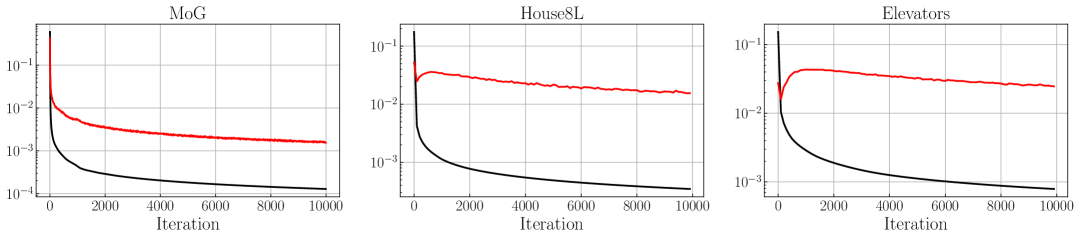
Figure 4: Empirical verification of Assumption˜5 on noise injection level $\beta_{t}$ used in all our experiments. The red line represents the left hand side of (10) and the black line represents the right hand side of (10).

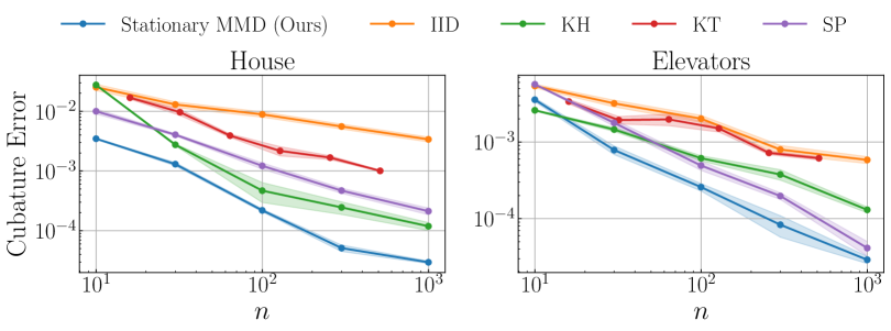
Figure 5: Ablation study of our stationary MMD points and all baselines using a Matérn-$\frac{3}{2}$ kernel on the House8L and Elevators datasets. The function used for cubature is $f_{1}(\bm{x})=\exp(-0.5\|\bm{x}\|^{2})$.

OpenML Datasets: We use House8L ($d=8$) dataset and Elevators ($d=18$) dataset from the OpenML database [Vanschoren et al., 2014] where the target distribution $\mu$ is the discrete measure corresponding to the full dataset. The ground truth cubature value is the empirical average of $f_{1}$ over the whole dataset. Both dataset are normalized to have zero mean and unit standard deviation. As a result, we fix the kernel lengthscale to $\ell=1$, rather than using the common heuristic of setting it to the median pairwise Euclidean distance. Our stationary MMD points are computed by simulating noisy MMD particle descent in (9) for $T=10000$ iterations. We adopt a fixed step size $\gamma=1.0$ for House8L dataset and $\gamma=0.3$ for Elevators dataset. We use a noise injection schedule $\beta_{t}=t^{-0.5}$. All baselines use the same kernel as stationary MMD points and their implementations are identical as the mixture of Gaussian experiment.

In Figure˜5, we present an ablation study of our stationary MMD points, KH (kernel herding) and KT (kernel thinning) using a Matérn-$\frac{3}{2}$ kernel. The Matérn-$\frac{3}{2}$ kernel satisfies all Assumptions˜1, 4 and 3 required for our stationary MMD points. SP (support points) remains the same because it does not involve choice of kernels [Mak and Joseph, 2018]. The results are consistent with those obtained using Gaussian kernels in the main text. Notably, for our stationary MMD points, the Matérn-$\frac{3}{2}$ kernel even outperforms the Gaussian kernel on the House8L dataset. A more comprehensive investigation of kernel choices is left for future work.

References

- Altekrüger et al. [2023] F. Altekrüger, J. Hertrich, and G. Steidl. Neural Wasserstein gradient flows for discrepancies with Riesz kernels. In 40th International Conference on Machine Learning, pages 664–690, 2023.
- Arbel et al. [2018] M. Arbel, D. J. Sutherland, M. Binkowski, and A. Gretton. On gradient regularizers for MMD GANs. In Advances in Neural Information Processing Systems, volume 31, pages 6701–6711, 2018.
- Arbel et al. [2019] M. Arbel, A. Korba, A. Salim, and A. Gretton. Maximum mean discrepancy gradient flow. In Advances in Neural Information Processing Systems, volume 32, pages 6484–6494, 2019.
- Aronszajn [1950] N. Aronszajn. Theory of reproducing kernels. Transactions of the American Mathematical Society, 68(3):337–404, 1950.
- Bach [2017] F. Bach. On the equivalence between kernel quadrature rules and random feature expansions. Journal of Machine Learning Research, 18(21):1–38, 2017.
- Bach et al. [2012] F. Bach, S. Lacoste-Julien, and G. Obozinski. On the equivalence between herding and conditional gradient algorithms. In 29th International Coference on Machine Learning, pages 1355–1362, 2012.
- Bachem et al. [2017] O. Bachem, M. Lucic, and A. Krause. Practical coreset constructions for machine learning. arXiv preprint arXiv:1703.06476, 2017.
- Bakhvalov [2015] N. S. Bakhvalov. On the approximate calculation of multiple integrals. Journal of Complexity, 31(4):502–516, 2015. English translation. Original; Vestnik MGU, Ser. Math. Mech. Astron. Phys. Chem., 4:3–18, 1959.
- Banerjee et al. [2025] S. Banerjee, K. Balasubramanian, and P. Ghosal. Improved finite-particle convergence rates for Stein variational gradient descent. In 13th International Conference on Learning Representations, 2025.
- Bardenet and Hardy [2020] R. Bardenet and A. Hardy. Monte Carlo with determinantal point processes. The Annals of Applied Probability, 30(1):368–417, 2020.
- Barp et al. [2024] A. Barp, C.-J. Simon-Gabriel, M. Girolami, and L. Mackey. Targeted separation and convergence with kernel discrepancies. Journal of Machine Learning Research, 25(378):1–50, 2024.
- Belhadji [2021] A. Belhadji. An analysis of Ermakov-Zolotukhin quadrature using kernels. In Advances in Neural Information Processing Systems, volume 34, pages 27278–27289, 2021.
- Belhadji et al. [2019] A. Belhadji, R. Bardenet, and P. Chainais. Kernel quadrature with DPPs. In Advances in Neural Information Processing Systems, volume 32, pages 12927–12937, 2019.
- Belhadji et al. [2025] A. Belhadji, D. Sharp, and Y. Marzouk. Weighted quantization using MMD: From mean field to mean shift via gradient flows. arXiv preprint arXiv:2502.10600, 2025.
- Berlinet and Thomas-Agnan [2004] A. Berlinet and C. Thomas-Agnan. Reproducing Kernel Hilbert Spaces in Probability and Statistics. Springer Science+Business Media, New York, 2004.
- Bottou et al. [2018] L. Bottou, F. E. Curtis, and J. Nocedal. Optimization methods for large-scale machine learning. SIAM Review, 60(2):223–311, 2018.
- Boufadène and Vialard [2023] S. Boufadène and F.-X. Vialard. On the global convergence of Wasserstein gradient flow of the Coulomb discrepancy. arXiv preprint arXiv:2312.00800, 2023.
- Boyd and Vandenberghe [2004] S. P. Boyd and L. Vandenberghe. Convex Optimization. Cambridge University Press, 2004.
- Brauchart and Grabner [2015] J. S. Brauchart and P. J. Grabner. Distributing many points on spheres: Minimal energy and designs. Journal of Complexity, 31(3):293–326, 2015.
- Briol et al. [2019] F.-X. Briol, C. J. Oates, M. Girolami, M. A. Osborne, and D. Sejdinovic. Probabilistic integration: A role in statistical computation? Statistical Science, 34(1):1–22, 2019.
- Briol et al. [2025] F.-X. Briol, A. Gessner, T. Karvonen, and M. Mahsereci. A dictionary of closed-form kernel mean embeddings. arXiv preprint arXiv:2504.18830, 2025.
- Carmeli et al. [2010] C. Carmeli, E. De Vito, A. Toigo, and V. Umanitá. Vector-valued reproducing kernel Hilbert spaces and universality. Analysis and Applications, 8(01):19–61, 2010.
- Chatalic et al. [2023] A. Chatalic, N. Schreuder, E. De Vito, and L. Rosasco. Efficient numerical integration in reproducing kernel Hilbert spaces via leverage scores sampling. arXiv preprint arXiv:2311.13548, 2023.
- Chen et al. [2010] Y. Chen, M. Welling, and A. Smola. Super-samples from kernel herding. In 26th Conference on Uncertainty in Artificial Intelligence, pages 109–116, 2010.
- Chen et al. [2021] Y. Chen, Y. Wang, L. Kang, and C. Liu. A deterministic sampling method via maximum mean discrepancy flow with adaptive kernel. arXiv preprint arXiv:2111.10722, 2021.
- Chen et al. [2024] Z. Chen, A. Mustafi, P. Glaser, A. Korba, A. Gretton, and B. K. Sriperumbudur. (De)-regularized maximum mean discrepancy gradient flow. arXiv preprint arXiv:2409.14980, 2024.
- Chen et al. [2025] Z. Chen, M. Naslidnyk, and F.-X. Briol. Nested expectations with kernel quadrature. arXiv preprint arXiv:2502.18284, 2025.
- Chopin and Gerber [2024] N. Chopin and M. Gerber. Higher-order Monte Carlo through cubic stratification. SIAM Journal on Numerical Analysis, 62(1):229–247, 2024.
- Delyon and Portier [2016] B. Delyon and F. Portier. Integral approximation by kernel smoothing. Bernoulli, 22(4):2177–2208, 2016.
- Dick and Pillichshammer [2010] J. Dick and F. Pillichshammer. Digital Nets and Sequences: Discrepancy Theory and Quasi–Monte Carlo Integration. Cambridge University Press, 2010.
- Dudley [2014] R. M. Dudley. Uniform Central Limit Theorems. Cambridge University Press, 2014.
- Duong et al. [2024] R. Duong, V. Stein, R. Beinert, J. Hertrich, and G. Steidl. Wasserstein gradient flows of MMD functionals with distance kernel and Cauchy problems on quantile functions. arXiv preprint arXiv:2408.07498, 2024.
- Dwivedi and Mackey [2024] R. Dwivedi and L. Mackey. Kernel thinning. Journal of Machine Learning Research, 25(152):1–77, 2024.
- Ehler et al. [2019] M. Ehler, M. Gräf, and C. J. Oates. Optimal Monte Carlo integration on closed manifolds. Statistics and Computing, 29(6):1203–1214, 2019.
- Fasshauer [2011] G. E. Fasshauer. Positive definite kernels: Past, present and future. Dolomites Research Notes on Approximation, 4:21–63, 2011.
- Galashov et al. [2025] A. Galashov, V. D. Bortoli, and A. Gretton. Deep MMD gradient flow without adversarial training. In 13th International Conference on Learning Representations, 2025. URL https://openreview.net/forum?id=Pf85K2wtz8.
- Gautier et al. [2019a] G. Gautier, R. Bardenet, and M. Valko. On two ways to use determinantal point processes for Monte Carlo integration. In Advances in Neural Information Processing Systems, volume 32, 2019a. URL https://proceedings.neurips.cc/paper_files/paper/2019/file/1d54c76f48f146c3b2d66daf9d7f845e-Paper.pdf.
- Gautier et al. [2019b] G. Gautier, G. Polito, R. Bardenet, and M. Valko. DPPy: DPP sampling with python. Journal of Machine Learning Research, 20(180):1–7, 2019b.
- Glaser et al. [2021] P. Glaser, M. Arbel, and A. Gretton. KALE flow: A relaxed KL gradient flow for probabilities with disjoint support. In Advances in Neural Information Processing Systems, volume 34, pages 8018–8031, 2021.
- Grabner [2014] P. Grabner. Point sets of minimal energy. In Applications of Algebra and Number Theory (Lectures on the Occasion of Harald Niederreiter’s 70th Birthday), pages 109–125. Cambridge University Press, 2014.
- Gretton et al. [2012] A. Gretton, K. M. Borgwardt, M. J. Rasch, B. Schölkopf, and A. Smola. A kernel two-sample test. Journal of Machine Learning Research, 13(1):723–773, 2012.
- Hayakawa and Morimura [2024] S. Hayakawa and T. Morimura. Policy gradient with kernel quadrature. Transactions on Machine Learning Research, 2024.
- Hayakawa et al. [2022] S. Hayakawa, H. Oberhauser, and T. Lyons. Positively weighted kernel quadrature via subsampling. In Advances in Neural Information Processing Systems, volume 35, pages 6886–6900, 2022.
- He et al. [2024] Y. He, K. Balasubramanian, B. K. Sriperumbudur, and J. Lu. Regularized Stein variational gradient flow. Foundations of Computational Mathematics, 2024.
- Hertrich et al. [2024a] J. Hertrich, M. Gräf, R. Beinert, and G. Steidl. Wasserstein steepest descent flows of discrepancies with Riesz kernels. Journal of Mathematical Analysis and Applications, 531(1):127829, 2024a.
- Hertrich et al. [2024b] J. Hertrich, C. Wald, F. Altekrüger, and P. Hagemann. Generative sliced MMD flows with Riesz kernels. In 12th International Conference on Learning Representations, 2024b. URL https://openreview.net/forum?id=VdkGRV1vcf.
- Hickernell [1998] F. Hickernell. A generalized discrepancy and quadrature error bound. Mathematics of Computation, 67(221):299–322, 1998.
- Hough et al. [2006] J. B. Hough, M. Krishnapur, Y. Peres, and B. Virág. Determinantal processes and independence. Probability Surveys, 3:206–229, 2006.
- Huszár and Duvenaud [2012] F. Huszár and D. Duvenaud. Optimally-weighted herding is Bayesian quadrature. In 28th Conference on Uncertainty in Artificial Intelligence, pages 377–386, 2012.
- Jagadeeswaran and Hickernell [2019] R. Jagadeeswaran and F. J. Hickernell. Fast automatic Bayesian cubature using lattice sampling. Statistics and Computing, 29(6):1215–1229, 2019.
- Karvonen [2022] T. Karvonen. Error bounds and the asymptotic setting in kernel-based approximation. Dolomites Research Notes on Approximation, 15(3):65–77, 2022.
- Karvonen and Särkkä [2018] T. Karvonen and S. Särkkä. Fully symmetric kernel quadrature. SIAM Journal on Scientific Computing, 40(2):A697–A720, 2018.
- Karvonen et al. [2018] T. Karvonen, C. J. Oates, and S. Särkkä. A Bayes-Sard cubature method. In Advances in Neural Information Processing Systems, volume 31, 2018.
- Karvonen et al. [2019a] T. Karvonen, M. Kanagawa, and S. Särkkä. On the positivity and magnitudes of Bayesian quadrature weights. Statistics and Computing, 29:1317–1333, 2019a.
- Karvonen et al. [2019b] T. Karvonen, S. Särkkä, and C. J. Oates. Symmetry exploits for Bayesian cubature methods. Statistics and Computing, 29:1231–1248, 2019b.
- Klebanov and Sullivan [2023] I. Klebanov and T. J. Sullivan. Transporting higher-order quadrature rules: Quasi-Monte Carlo points and sparse grids for mixture distributions. arXiv preprint arXiv:2308.10081, 2023.
- Korba et al. [2020] A. Korba, A. Salim, M. Arbel, G. Luise, and A. Gretton. A non-asymptotic analysis for Stein variational gradient descent. In Advances in Neural Information Processing Systems, volume 33, pages 4672–4682, 2020.
- Krieg and Sonnleitner [2024] D. Krieg and M. Sonnleitner. Random points are optimal for the approximation of Sobolev functions. IMA Journal of Numerical Analysis, 44(3):1346–1371, 2024.
- Larkin [1972] F. Larkin. Gaussian measure in Hilbert space and applications in numerical analysis. The Rocky Mountain Journal of Mathematics, pages 379–421, 1972.
- Lee [2012] J. M. Lee. Introduction to Smooth Manifolds. Springer, 2012. ISBN 9781441999825. doi: https://doi.org/10.1007/978-1-4419-9982-5.
- Leluc et al. [2025] R. Leluc, F. Portier, J. Segers, and A. Zhuman. Speeding up Monte Carlo integration: Control neighbors for optimal convergence. Bernoulli, 31(2):1160–1180, 2025.
- Lemieux [2004] C. Lemieux. Randomized quasi-Monte carlo: A tool for improving the efficiency of simulations in finance. In 2004 Winter Simulation Conference 2004, volume 2, pages 1565–1573. IEEE, 2004.
- Liu and Wang [2016] Q. Liu and D. Wang. Stein variational gradient descent: A general purpose Bayesian inference algorithm. In Advances in Neural Information Processing Systems, volume 29, 2016.
- Liu and Wang [2018] Q. Liu and D. Wang. Stein variational gradient descent as moment matching. In Advances in Neural Information Processing Systems, volume 31, 2018.
- Mak and Joseph [2018] S. Mak and V. R. Joseph. Support points. The Annals of Statistics, 46(6A):2562–2592, 2018.
- Marzo and Mas [2021] J. Marzo and A. Mas. Discrepancy of minimal Riesz energy points. Constructive Approximation, 54(3):473–506, 2021.
- Novak [1988] E. Novak. Deterministic and stochastic error bounds in numerical analysis. 1988.
- Oates et al. [2017] C. J. Oates, M. Girolami, and N. Chopin. Control functionals for Monte Carlo integration. Journal of the Royal Statistical Society Series B: Statistical Methodology, 79(3):695–718, 2017.
- Oettershagen [2017] J. Oettershagen. Construction of Optimal Cubature Algorithms with Applications to Econometrics and Uncertainty Quantification. PhD thesis, Universität Bonn, 2017.
- Paulsen and Raghupathi [2016] V. I. Paulsen and M. Raghupathi. An Introduction to the Theory of Reproducing Kernel Hilbert Spaces. Cambridge University Press, 2016.
- Philippe and Robert [2001] A. Philippe and C. P. Robert. Riemann sums for MCMC estimation and convergence monitoring. Statistics and Computing, 11:103–115, 2001.
- Rudin [1976] W. Rudin. Principles of Mathematical Analysis, 3rd Edition. McGraw-Hill New York, 1976.
- Santin et al. [2021] G. Santin, T. Karvonen, and B. Haasdonk. Sampling based approximation of linear functionals in reproducing kernel Hilbert spaces. BIT Numerical Mathematics, 62:279–310, 2021.
- Schaback [1999] R. Schaback. Improved error bounds for scattered data interpolation by radial basis functions. Mathematics of Computation, 68(225):201–216, 1999.
- Schaback [2018] R. Schaback. Superconvergence of kernel-based interpolation. Journal of Approximation Theory, 235:1–19, 2018.
- Sejdinovic et al. [2013] D. Sejdinovic, B. Sriperumbudur, A. Gretton, and K. Fukumizu. Equivalence of distance-based and RKHS-based statistics in hypothesis testing. The Annals of Statistics, 41(5):2263–2291, 2013.
- Shetty et al. [2022] A. Shetty, R. Dwivedi, and L. Mackey. Distribution compression in near-linear time. In 10th International Conference on Learning Representations, 2022. URL https://openreview.net/forum?id=lzupY5zjaU9.
- Shi and Mackey [2024] J. Shi and L. Mackey. A finite-particle convergence rate for Stein variational gradient descent. In Advances in Neural Information Processing Systems, volume 36, pages 26831–26844, 2024.
- Sloan and Kaarnioja [2025] I. H. Sloan and V. Kaarnioja. Doubling the rate: Improved error bounds for orthogonal projection with application to interpolation. BIT Numerical Mathematics, 65(1):10, 2025.
- Sloan and Womersley [2009] I. H. Sloan and R. S. Womersley. A variational characterisation of spherical designs. Journal of Approximation Theory, 159(2):308–318, 2009.
- Smola et al. [2007] A. Smola, A. Gretton, L. Song, and B. Schölkopf. A Hilbert space embedding for distributions. In 18th International Conference on Algorithmic Learning Theory, pages 13–31, 2007.
- Sriperumbudur et al. [2011] B. K. Sriperumbudur, K. Fukumizu, and G. R. Lanckriet. Universality, characteristic kernels and RKHS embedding of measures. Journal of Machine Learning Research, 12(7), 2011.
- Steinwart and Christmann [2008] I. Steinwart and A. Christmann. Support Vector Machines. Springer Science & Business Media, 2008.
- Teymur et al. [2021] O. Teymur, J. Gorham, M. Riabiz, and C. J. Oates. Optimal quantisation of probability measures using maximum mean discrepancy. In 24th International Conference on Artificial Intelligence and Statistics, pages 1027–1035, 2021.
- Traub et al. [1988] J. Traub, G. Wasilkowski, and H. Woźniakowski. Information-Based Complexity. Academic Press, 1988.
- Vanschoren et al. [2014] J. Vanschoren, J. N. Van Rijn, B. Bischl, and L. Torgo. OpenML: Networked science in machine learning. ACM SIGKDD Explorations Newsletter, 15(2):49–60, 2014.
- Xu et al. [2022] L. Xu, A. Korba, and D. Slepcev. Accurate quantization of measures via interacting particle-based optimization. In 39th International Conference on Machine Learning, pages 24576–24595, 2022.