‘Hello, World!’: Making GNNs Talk with LLMs

Abstract

While graph neural networks (GNNs) have shown remarkable performance across diverse graph-related tasks, their high-dimensional hidden representations render them black boxes. In this work, we propose Graph Lingual Network (GLN), a GNN built on large language models (LLMs), with hidden representations in the form of human-readable text. Through careful prompt design, GLN incorporates not only the message passing module of GNNs but also advanced GNN techniques, including graph attention and initial residual connection. The comprehensibility of GLN’s hidden representations enables an intuitive analysis of how node representations change (1) across layers and (2) under advanced GNN techniques, shedding light on the inner workings of GNNs. Furthermore, we demonstrate that GLN achieves strong zero-shot performance on node classification and link prediction, outperforming existing LLM-based baseline methods.

‘Hello, World!’: Making GNNs Talk with LLMs

Sunwoo Kim¹   Soo Yong Lee¹   Jaemin Yoo²   Kijung Shin^{1,2 1}Kim Jaechul Graduate School of AI, KAIST,  ²School of Electrical Engineering, KAIST {kswoo97, syleetolow, jaemin, kijungs}@kaist.ac.kr

1 Introduction

Graph neural networks (GNNs) are designed to process graph-structured data, and they have demonstrated strong performance in various downstream tasks such as node classification and link prediction Corso et al. (2024). A key to their success lies in their message passing module, which updates the representation of a node by aggregating information from its neighbors Hamilton (2020). However, the high-dimensional embeddings (i.e., vectorized representations) obtained via existing GNNs are generally not comprehensible.

In this work, we propose GLN (Graph Lingual Network), where an LLM is prompted to aggregate neighbor information to update a node’s representation. Therefore, all hidden node representations of GLN are human-readable texts. Moreover, we propose a tailored LLM prompting framework incorporating advanced GNN techniques, specifically graph attention Veličković et al. (2018) and initial residual connection Chen et al. (2020).

Compared to existing GNNs, our GLN offers several advantages. First, its hidden representations are comprehensible and human-readable, since they are text descriptions of nodes generated by the LLM. Second, using an LLM as the message passing module enables GLN to solve graph-related tasks in a zero-shot manner, without any training or task labels. Third, GLN can be further prompted to explain its decisions on graph-related tasks, facilitating human understanding of its reasoning.

Thanks to the comprehensibility of GLN’s hidden representations, we provide an intuitive analysis regarding how the node representations change (1) across GLN layers and (2) under advanced GNN techniques. Drawing from this analysis, we offer several key insights into the mechanisms underlying GNN message passing and its advanced techniques. Moreover, we demonstrate the zero-shot capability of GLN on popular downstream tasks (node classification and link prediction), demonstrating its superiority over existing LLM-based baseline methods. Code and datasets are in https://github.com/kswoo97/GLN-Code.

2 Related work and preliminaries

In this section, we cover related work and preliminaries of our research.

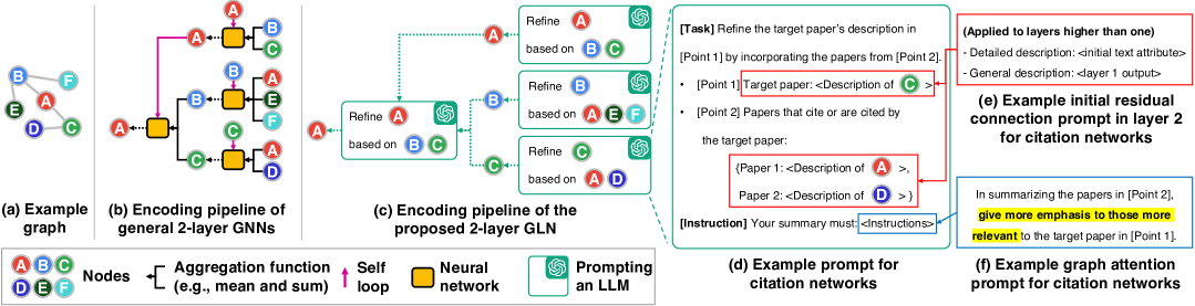
Figure 1: Overview of general GNNs and our GLN. To obtain node \textcolor{red}{\smallA}⃝’s representation in example graph (a), a general 2-layer GNN first refines the representations of \textcolor{red}{\smallA}⃝ and its one-hop neighbors, and then updates that of \textcolor{red}{\smallA}⃝ again using these refined representations, as shown in (b). A similar mechanism is applied in GLN, as shown in (c), but the aggregation functions and neural networks are replaced by an LLM with our prompt, illustrated in (d) - (f).

2.1 Related work

Graph neural networks. In various graph-related tasks, such as node classification and link prediction, graph neural networks (GNNs) have achieved strong performance Luo et al. (2024). The core module of a GNN involves message-passing, which updates node representation by aggregating information from its neighboring nodes Hamilton (2020) (refer to Figure 1 (b) for an example). This process is typically repeated across layers, enabling a node’s representation at $k-$th layer to summarize its $k-$hop neighbor information.

Several advanced techniques have been proposed to enhance GNN message passing, notably graph attention Veličković et al. (2018) and initial residual connection Chen et al. (2020). Graph attention allows a GNN to learn the relative importance of each neighbor during aggregation. Initial residual connections help preserve original representations (i.e., initial feature vectors) by injecting them into each layer, mitigating their degradation by the repeated message passing.

Combining GNNs with LLMs. With the remarkable performance of LLMs in a wide range of domains Chang et al. (2024), many studies have combined them with GNNs to tackle various graph-related tasks Ren et al. (2024). Early works either fine-tuned LLMs Chen et al. (2024a) or fed LLM outputs into GNNs during their training for graph-related tasks He et al. (2024), both incurring high training costs. In contrast, several recent works prompted LLMs to model GNNs’ operations without further training Chen et al. (2024b); Zhu et al. (2025). Among them, Zhu et al. (2025) obtained graph vocabulary for graph foundation models by prompting LLMs to mimic the message-passing modules of GNNs. Since their method does not aim for user comprehension, the refined representations offer limited utility from a comprehension perspective. Specifically, instead of enriching textual representations of nodes across layers, it tends to merely enumerate neighbor information (see Appendix B.3 for details).

2.2 Preliminaries

A graph $\mathcal{G}=\{\mathcal{V},\mathcal{E}\}$ is defined by a node set $\mathcal{V}=\{v_{1},\cdots,v_{|\mathcal{V}|}\}$ and an edge set $\mathcal{E}=\{e_{1},\cdots,e_{|\mathcal{E}|}\}$. Each edge $e_{i}\in\mathcal{E}$ is defined by a pair of nodes (i.e., $e_{i}\in\binom{\mathcal{V}}{2}$), and node $v_{i}$’s neighbor set $\mathcal{N}_{i}$ is defined by a set of nodes linked to $v_{i}$ (i.e., $\mathcal{N}_{i}=\{v_{j}\in\mathcal{V}:\{v_{i},v_{j}\}\in\mathcal{E}\}$). In this work, we consider a text-attributed graph, where each node $v_{i}\in\mathcal{V}$ is associated with text attribute ${D}^{(0)}_{i}$ that describes $v_{i}$, which we call initial text attribute.

3 Proposed method: GLN

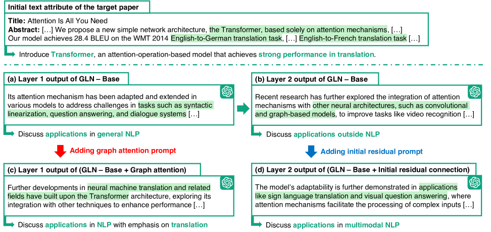
Figure 2: Representations become more general across layers, are specialized to the target node through graph attention, and retain target-specific information in higher layers through initial residual connections. We present a case study on (Vaswani et al., 2017), showing GLN-Base’s representations of the paper at: (a) layer 1, (b) layer 2, (c) layer 1 with a graph attention prompt, and (d) layer 2 with an initial residual connection prompt.

In this section, we introduce GLN (Graph Lingual Network), a graph neural network where an LLM serves as its message passing module. We first give an overview of GLN (Sec. 3.1) and describe our specialized prompt that incorporates GNNs’ advanced techniques (Sec. 3.2). Refer to Figure 1 for an overview of GLN.

3.1 Overview

At each layer, GLN refines the textual representation of each node by prompting an LLM to aggregate information from the node’s neighbors. Specifically, at layer $\ell$, an LLM receives an input prompt consisting of (1) the target node $v_{i}$’s representation from the previous layer $D^{(\ell-1)}_{i}$ and (2) the neighbor representations from the previous layer $\{D^{(\ell-1)}_{j}:v_{j}\in\mathcal{N}_{i}\}$ (the prompt design is detailed in Sec. 3.2).  The LLM then outputs the refined textual representation of $v_{i}$, denoted as $D^{(\ell)}_{i}$, effectively integrating the prior representations of both the target node and its neighbors.

After $L$ iterations, corresponding to the number of GLN layers, we define the final representation of node $v_{i}$ as the set of its intermediate embeddings (i.e., $\{D^{(t)}_{i}:t\in\{0,1,\cdots,L\}$) to capture diverse information about the node. Note that each layer of a GNN captures a different level of neighborhood information: the earlier layers encode fine-grained, local features from immediate neighbors, while the later layers aggregate broader and more abstract information from multi-hop neighbors Xu et al. (2018).

3.2 Advanced GNN-style prompting

The key innovation of GLN involves its prompt design, which determines how the LLM aggregates neighbor information to update the target node representation. To this end, we adopt two advanced GNN techniques: (1) graph attention Veličković et al. (2018) and (2) initial residual connection Chen et al. (2020) (refer to Sec. 2.1 for their details). To implement graph attention with an LLM, we design a prompt that encourages the LLM to place greater emphasis on neighbors that are more relevant to the target node during aggregation; we refer to this as the graph attention prompt (refer to Figure 1 (f)). Similarly, to implement initial residual connections, we include both the previous-layer output and the raw attributes of each node in their descriptions—we refer to this as the initial residual connection prompt (refer to Figure 1 (e)). The detailed prompt design is provided in Appendix D.1.

4 Analysis and experiments

LLMs	Methods	Task: Node classification			Task: Link prediction			A.R.
		OGBN-Arxiv	Book-History	Wiki-CS	OGBN-Arxiv	Book-History	Wiki-CS
GPT	Direct	62.3	44.7	78.3	92.8	85.0	83.2	3.8
	All-in-One	61.5	45.4	64.9	91.6	84.8	85.6	3.6
	PromptGFM	62.0	44.1	79.0	92.2	81.2	81.0	4.2
	GLN-Base	63.0	45.8	79.4	92.4	86.4	83.6	2.2
	GLN	64.0	47.3	79.5	93.0	87.0	84.0	1.2
Claude	Direct	65.8	48.4	76.6	78.0	65.2	41.2	3.2
	All-in-One	67.1	50.4	76.4	72.8	53.6	38.6	3.7
	PromptGFM	65.3	50.6	74.5	64.4	50.0	38.2	4.7
	GLN-Base	67.1	53.8	77.0	78.2	61.2	42.4	2.2
	GLN	67.4	55.2	77.7	78.4	64.0	43.2	1.2

Table 1: GLN outperforms the zero-shot LLM-based baselines on popular graph-related tasks. For node classification and link prediction, we report accuracy and Hit-ratio@1, respectively, of each method in each dataset. A.R. denotes average ranking. The best performance in each setting is highlighted in green.

In this section, we analyze representations obtained by GLN and demonstrate its zero-shot capability in several graph-related tasks.

4.1 Representation analysis

Setup. We conduct a case study of GLN representation of an academic paper, (Vaswani et al., 2017) (Figure 2), on the OGBN-arXiv citation network dataset Hu et al. (2020), where nodes and edges represent papers and citations, respectively. Additional examples from diverse domains (e.g., computer vision and graph learning) are in Appendix B.1. We extract layer-1 and layer-2 outputs of GLN-Base, a GLN variant that omits graph attention and initial residual connection prompts, using GPT-4o to analyze the effect of the message passing. To analyze the impact of the two GNN techniques, we also extract the paper’s GLN representation with the graph attention prompt and one with the initial residual connection prompt.

Observation 1. The node representations become more general across layers. As shown in Figure 2 (a) and (b), the layer-1 representation focuses on how the attention operation is used in the NLP domain. In the layer-2, the scope expands to applications of attention in computer vision and graph learning. This shift across GLN layers suggests that adding message-passing layers (i.e., incorporating information of the farther neighbors) makes each node’s representation more general.

Observation 2. Graph attention tailors the neighbor summary for the target node. As shown in Figure 2 (a) and (c), the paper representation obtained from GLN-Base involves non-specific enumeration of various NLP tasks. However, after applying the graph attention prompt, the representation involves the specific task addressed in the target paper. This result suggests that graph attention encourages aggregation toward neighbors that are more relevant to the target paper.

Observation 3. Initial residual connection preserves the target node information after message passing. As shown in Figure 2 (c) and (d), the representation obtained from GLN-Base describes application of the attention operation outside NLP, whereas the one obtained after applying the initial residual prompt maintains its focus on the NLP domain. This result suggests that the initial residual connection prompt preserves the target node’s initial text attribute, encouraging its updated representation to stay aligned with that context.

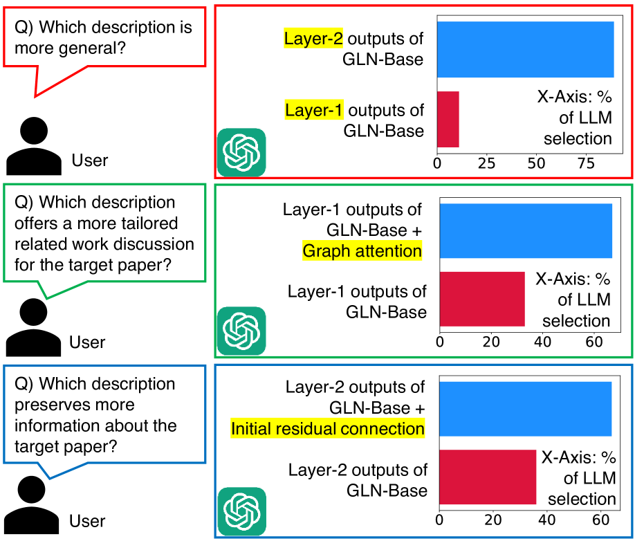
Figure 3: Observations 1-3 hold valid under the LLM-as-a-judge protocol. We report the ratio of LLM responses per category for each question.

Observation 4. Observations 1-3 are validated via LLM-as-a-judge protocol. We provide a quantitative assessment of our observations. To this end, we randomly sample $10^{2}$ papers and extract the four aforementioned representations for each. We then prompt GPT-4o to validate our observation on the representations, resulting in an evaluation consistent with our observations, as shown in Figure 3.

4.2 Zero-shot capability analysis

Setup. We use two backbone LLMs (GPT-4o-mini and Claude-3.0-Haiku) and three real-world graphs: a citation network (OGBN-arXiv), a co-purchase network (Book-History), and a hyperlink network (Wiki-CS), whose further details are in Appendix A. After obtaining the target node’s textual representation using the proposed method and baselines, we input it into an LLM to perform node classification and edge prediction. Detailed prompts for each task and further experimental details in Appendices D.3 and C.1, respectively.

Baseline methods and GLN. We use four baseline methods: (1) using only the initial text attribute of the target node (Direct), (2) providing one-hop and two-hop neighbors to the LLM to update the target node’s representation (All-in-One), (3) an existing text-attributed graph foundation model (PromptGFM) Zhu et al. (2025), and (4) a baseline version of GLN (GLN-Base). Further details regarding baselines and GLN are in Appendix C.2.

Results. GLN outperforms baseline methods in 10 out of 12 settings (Table 1), demonstrating its effectiveness in zero-shot capability in node classification and link prediction. Two points stand out: (1) GLN ’s superior performance over Direct highlights the effectiveness of utilizing graph topology, and (2) its gain over GLN-Base shows the effectiveness of our advanced GNN-style prompts. Further ablation study results are in Appendix B.4.

LLM Reasoning. We further analyze the LLM’s reasoning behind its downstream task decisions in Appendix B.2, highlighting which parts of the textual representation contribute to performance.

5 Conclusion

We propose GLN, a GNN that uses an LLM as its message passing module. Leveraging the comprehensibility of its hidden representations, we provide intuitive insights into message passing and advanced GNN techniques. Moreover, GLN outperforms baselines on zero-shot graph-related tasks.

Limitations

Theoretical property. Various theoretical properties of graph neural networks, such as expressivity Xu et al. (2019) and permutation invariance Keriven and Peyré (2019), have been widely studied. However, the complex nature of large language models makes understanding the theoretical properties of GLN challenging and remains unexplored in this work. Therefore, investigating the theoretical foundations of GLN is a promising direction for future research.

Computational efficiency compared to GNNs. Due to the usage of a large language model, GLN has significantly more parameters than general GNNs, which return vectorized node representations. Therefore, exploring scaled-up versions of GLN can be a promising direction for future work.

LLM API Cost. We used LLM APIs (specifically, GPT-4o, GPT-4o-mini, and Claude-3.0-Haiku), incurring a total cost of approximately $600 for this research. This may hinder broader accessibility and practical use in budget-constrained environments. Developing token-efficient prompting could significantly reduce cost and enable broader applicability of our approach.

Appendix A Dataset details

Dataset	#Nodes	#Edges	#Classes
OGBN-Arxiv	169,343	1,166,243	40
Book-History	41,551	358,574	12
Wiki-CS	11,701	216,123	10

Table 2: Graph statistics of the datasets.

In this appendix section, we provide details regarding the datasets used in this work. The detailed statistics of each dataset is provided in Table 2.

OGBN-Arxiv Hu et al. (2020) is a citation network that represents the citation relations between papers. In this dataset, each node corresponds to a particular paper, and edges join the papers that cite or are cited by the corresponding paper. The attributes of a node correspond to the title and abstract of the corresponding node (paper). The class of a node corresponds to the arXiv category to which the corresponding node (paper) belongs.

Book-History Yan et al. (2023) is a co-purchase network that represents the co-purchase relations among books. In this dataset, each node corresponds to a particular book, and edges join the books that are frequently co-purchased together with the corresponding book. The attributes of a node correspond to the description of the corresponding node (book). The class of a node corresponds to the Amazon third-level category to which the corresponding node (book) belongs.

Wiki-CS Mernyei and Cangea (2020) is a hyperlink network that represents the hyperlink relations among Wikipedia web pages. In this dataset, each node corresponds to a particular Wikipedia web page, and edges join the pages that are either hyperlinked to or from the corresponding page. The attributes of a node correspond to the content within the corresponding node (web page). The class of a node corresponds to the Wikipedia category to which the corresponding node (web page) belongs.

Appendix B Additional analysis

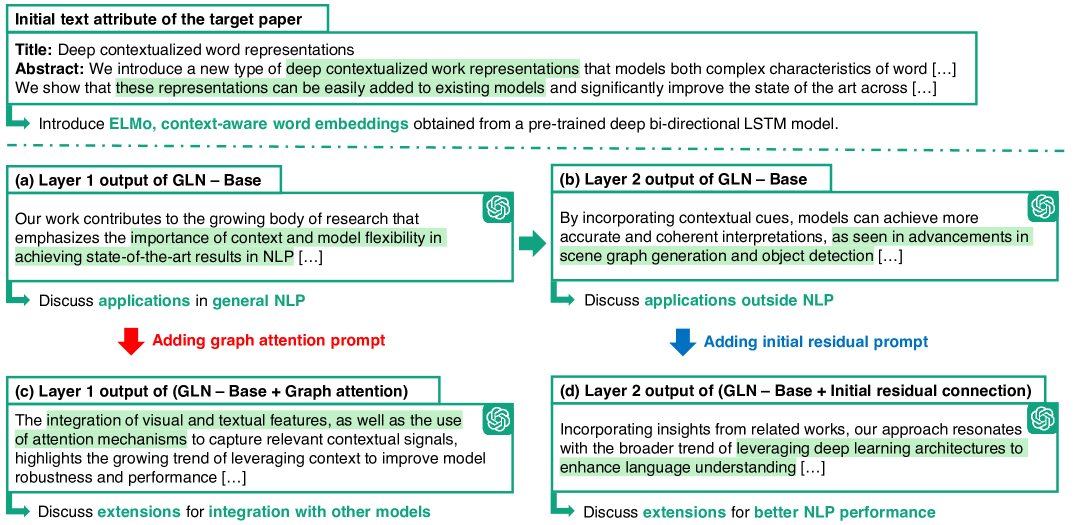
Figure 4: A case study on (Peters et al., 2018), showing GLN-Base’s representations of the paper at: (a) layer 1, (b) layer 2, (c) layer 1 with a graph attention prompt, and (d) layer 2 with an initial residual connection prompt.

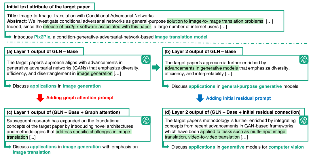
Figure 5: A case study on (Isola et al., 2017), showing GLN-Base’s representations of the paper at: (a) layer 1, (b) layer 2, (c) layer 1 with a graph attention prompt, and (d) layer 2 with an initial residual connection prompt.

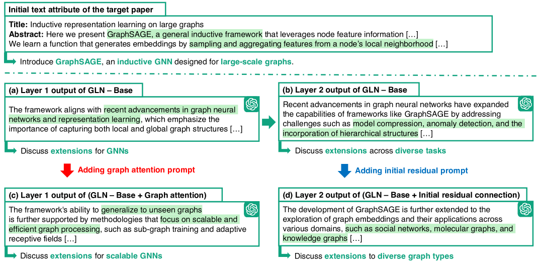
Figure 6: A case study on (Hamilton et al., 2017), showing GLN-Base’s representations of the paper at: (a) layer 1, (b) layer 2, (c) layer 1 with a graph attention prompt, and (d) layer 2 with an initial residual connection prompt.

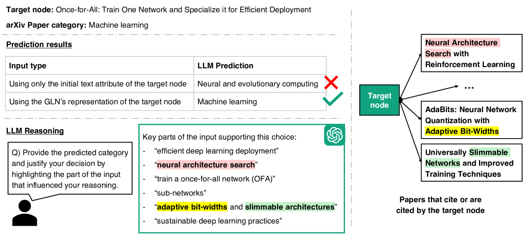
Figure 7: A case study on (Cai et al., 2020), showing LLM’s reasoning for its downstream task decision. While an LLM misclassified the target node when only using the node attributes, it correctly classifies the target node by using information obtained from the target node’s neighbors.

Figure 8: A case study on (Talak and Modiano, 2020), showing LLM’s reasoning for its downstream task decision. While an LLM misclassified the target node when only using the node attributes, it correctly classifies the target node by using information obtained from the target node’s neighbors.

In this appendix section, we provide additional experimental results that are omitted from the main section due to space constraints. Specifically, we present two types of case studies: Case studies analyzing representations of GLN in various domains (Appendix B.1) and case studies analyzing the reasoning of GLN on downstream graph-related tasks (Appendix B.2).

B.1 Representation analysis

We analyze the three popular papers from the three different domains:

• Natural language processing (NLP): ELMo, a pre-trained language model (Peters et al., 2018)

• Computer vision (CV): Pix2Pix, an image translation generative model (Isola et al., 2017)

• Graph representation learning (GRL): GraphSAGE, an inductive graph neural network model (Hamilton et al., 2017)

NLP Paper: ELMo. The case study result for ELMo (Peters et al., 2018) is presented in Figure 4. Below, we analyze whether the observations in Section 4.1 are valid in (Peters et al., 2018).

• Observation 1. As shown in Figure 4 (a) and (b), the layer-1 output focuses on the applications of context learning in NLP, while the layer-2 output extends to applications beyond NLP, such as scene graph generation and object detection. This result suggests that the representation gets more general across layers.

• Observation 2. As shown in Figure 4 (a) and (c), the output without the graph attention prompt lists applications of context learning in NLP, whereas the output with the prompt focuses on the integration of contextualized embeddings with additional features—a technique emphasized in the target paper. This result suggests that the representation gets specialized with the graph attention prompt.

• Observation 3. As shown in Figure 4 (b) and (d), the output without the initial residual connection prompt discusses the applications of context learning in various domains, while that with the initial residual connection prompt focuses on the architectural progress in NLP, domain where the target paper belongs to. This result suggests that the initial residual connection prompt helps maintain the information provided from the initial text attribute.

In summary, our analysis result suggests that the observations in Section 4.1 are still valid in (Peters et al., 2018).

CV Paper: Pix2Pix. The case study result for Pix2Pix (Isola et al., 2017) is presented in Figure 5. Below, we analyze whether the observations in Section 4.1 are valid in (Isola et al., 2017).

• Observation 1. As shown in Figure 5 (a) and (b), the layer-1 output focuses on the extensions of pix2pix in image generation, while the layer-2 output discusses its extensions for general generative models, without targeting specific domain. This result suggests that the representation gets more general across layers.

• Observation 2. As shown in Figure 5 (a) and (c), the output without the graph attention prompt covers image generation, whereas the output with the prompt focuses on the image translation within image generation, a task the target paper focuses on. This result suggests that the representation gets specialized with the graph attention prompt.

• Observation 3. As shown in Figure 5 (b) and (d), the output without the initial residual connection prompt discusses the general generative models, while that with the initial residual connection prompt focuses on the generative models for computer vision, which is the key domain the target paper belongs to. This result suggests that the initial residual connection prompt helps maintain the information provided from the initial text attribute.

In summary, our analysis result suggests that the observations in Section 4.1 are still valid in (Isola et al., 2017).

GRL Paper: GraphSAGE. The case study result for GraphSAGE (Hamilton et al., 2017) is presented in Figure 6. Below, we analyze whether the observations in Section 4.1 are valid in (Hamilton et al., 2017).

• Observation 1. As shown in Figure 6 (a) and (b), the layer-1 output focuses on the extensions of GraphSAGE for graph neural networks, while the layer-2 output covers the diverse applications of GraphSAGE, such as model compression and anomaly detection. This result suggests that the representation gets more general across layers.

• Observation 2. As shown in Figure 6 (a) and (c), the output without the graph attention prompt covers the extensions of GraphSAGE for general-purpose GNNs, while that with the prompt focuses on the inductive and/or scalable GNNs, which are key characteristics of GraphSAGE. This result suggests that the representation gets specialized with the graph attention prompt.

• Observation 3. As shown in Figure 6 (b) and (d), the output without the initial residual connection prompt discusses GraphSAGE applications across various tasks, whereas the output with the prompt emphasizes its use with different graph types, aligning with the target paper’s broader focus on graph representation learning. This result suggests that the initial residual connection prompt helps maintain the information provided from the initial text attribute.

In summary, our analysis result suggests that the observations in Section 4.1 are still valid in (Hamilton et al., 2017).

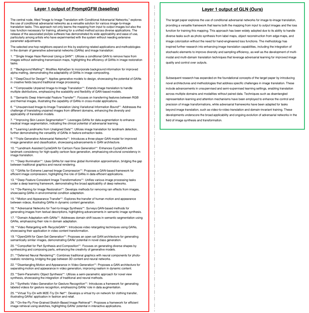
Figure 9: A case study on (Isola et al., 2017). While PromptGFM outputs a straightforward list of citing and cited papers, GLN offers a comprehensible and succinct summary of those closely related to the target paper.

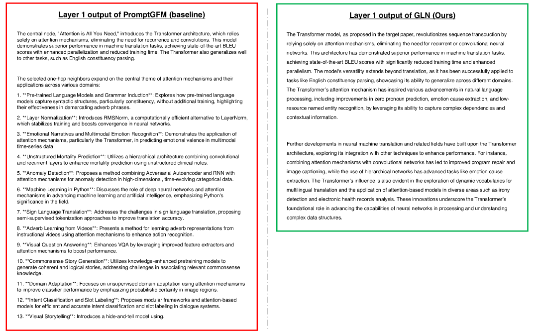
Figure 10: A case study on (Vaswani et al., 2017). While PromptGFM outputs a straightforward list of citing and cited papers, GLN offers a comprehensible and succinct summary of those closely related to the target paper.

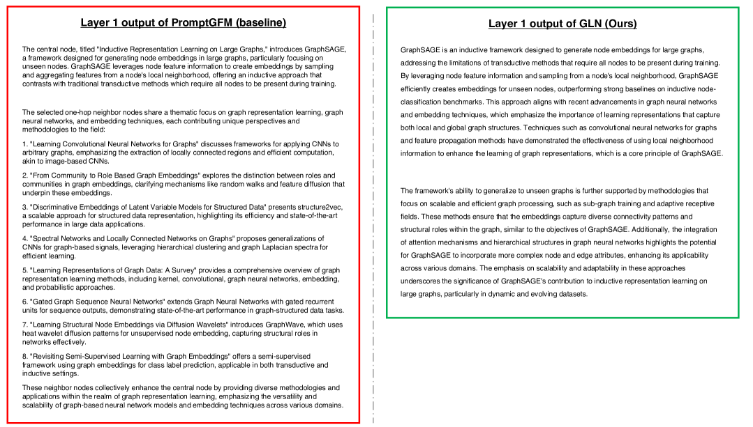
Figure 11: A case study on (Hamilton et al., 2017). While PromptGFM outputs a straightforward list of citing and cited papers, GLN offers a comprehensible and succinct summary of those closely related to the target paper.

B.2 Reasoning analysis

As noted in Section 1, textual representations allow an LLM to reason about its downstream task decisions. In this section, we present case studies on two papers in the arXiv dataset where using only the initial text attribute results in misclassification, while using the representation from GLN yields correct classification.

Case study 1. The first case is about (Cai et al., 2020). As shown in Figure 7, the LLM misclassifies the target node when relying solely on its initial textual attributes (title and abstract) but correctly classifies it when using the representation from GLN, where the correct label is ’machine learning‘. Notably, the LLM explicitly references terms from neighboring nodes (e.g., neural architecture search, slimmable networks) that are closely associated with the machine learning’ category. This reasoning result suggests that integrating neighbor information can improve node classification performance, and GLN effectively represents it.

Case study 2. The second case is about (Talak and Modiano, 2020). As shown in Figure 7, the LLM misclassifies the target node when relying solely on its initial text attributes (title and abstract) but correctly classifies it when using the representation from GLN, where the correct label is ‘networking and internet architecture’. Notably, the LLM explicitly references terms from neighboring nodes (e.g., age of information, scheduling, and queueing) that are closely associated with the networking and internet architecture category. This reasoning result suggests that integrating neighbor information can improve node classification performance, and GLN effectively represents it.

B.3 Comparison with PromptGFM

Recall that we briefly discussed the comparison between the outputs of GLN and that of PromptGFM Zhu et al. (2025), which is a baseline method (Section 2.1). In this section, we provide a detailed case study that compares (1) the representations obtained via PromptGFM and (2) those obtained via GLN.

Setup. To this end, we present the first-layer outputs of PromptGFM and GLN for three papers from different domains within the arXiv citation network: (Isola et al., 2017) (CV), (Vaswani et al., 2017) (NLP), and (Hamilton et al., 2017) (GRL). We use GPT-4o as the backbone LLM for both methods.

Results. In short, the output of GLN is more comprehensible and well-structured, whereas that of PromptGFM is limited in its utility from a user comprehension perspective. Specifically, as shown in Figure 9, representations from PromptGFM list brief summaries of papers that cite or are cited by the target paper (Isola et al., 2017). In contrast, GLN returns a concise and focused summary of the target node’s neighbors, highlighting how generative adversarial networks (GANs) are applied to image translation tasks and further developed.

Similar results are shown in the outputs for (Vaswani et al., 2017) and (Hamilton et al., 2017), as shown in Figure 10 and Figure 11, respectively. These results suggest that GLN yields clearer, better-structured outputs, whereas PromptGFM’s are far less useful for user comprehension.

Potential reasons. We hypothesize that the differences in user comprehensibility primarily arise from the specific task assigned to the LLM. Specifically, PromptGFM prompts an LLM to ‘aggregate neighbor nodes and update a concise yet meaningful representation for the central node’. This prompt likely leads the LLM to focus heavily on aggregating neighbor information, resulting in a mere enumeration of the target node’s neighbors.

In contrast, in GLN, we prompt an LLM to refine the target node’s description by incorporating its neighbor information. This guides the LLM to center its attention on the target node and produce a target-node-centric summary of its neighbors, enhancing the overall user comprehensibility of the output text.

B.4 Ablation study

In this section, we provide further ablation studies of GLN: demonstrating whether each (1) graph attention prompt and (2) initial residual connection prompt is effective for the downstream task.

As shown in Table 3, GLN —which incorporates both graph attention and initial residual connection prompts—outperforms all three variants that omit either or both prompts. This result suggests that the two advanced GNN-style prompts are essential for good downstream task performance.

G.A.	I.R.C.	OGBN-arXiv		Book-History
		Node.	Link.	Node.	Link.
✗	✗	63.0	92.4	45.8	86.4
✓	✗	62.8	92.4	47.0	86.6
✗	✓	63.5	92.2	46.7	86.4
✓	✓	64.0	93.0	47.3	87.0

Table 3: Graph attention prompt and initial residual connection prompt are essential for strong performance. Ablation study result of GLN. G.A. and I.R.C. denote the graph attention prompt and the initial residual prompt connection prompt, respectively. In addition, Node. and Link. denote node classification and link prediction, respectively. The best performance in each setting is highlighted in bold.

Appendix C Experiment details

In this appendix section, we provide experimental details omitted from the main paper (Section 4).

C.1 Experimental setting details

We describe the detailed experimental setting of the two downstream tasks: (1) node classification and (2) link prediction.

Node classification. For node classification, we sample 1,000 nodes with degrees greater than or equal to 10 from each dataset (i.e., $\{v_{i}\in\mathcal{V}:|\mathcal{N}_{i}|\geq 10\}$). We then obtain the textual representations of the corresponding nodes and prompt an LLM to predict their classes. Lastly, measure accuracy by comparing the predicted classes with the ground-truth classes.

Link prediction. For link prediction, we sample 500 edges whose endpoint nodes each have a degree greater than 10 (i.e., $\{e_{i}=\{v_{s},v_{t}\}\in\mathcal{E}:|\mathcal{N}_{s}|,|\mathcal{N}_{t}|\geq 10\}$). We then remove these edges from $\mathcal{E}$ and obtain the textual representations of their endpoint nodes. Next, for each edge, we: (1) randomly sample four nodes not connected by the edge using rule-based sampling, (2) provide one endpoint of the edge as input to the LLM, (3) construct a candidate set consisting of the true other endpoint and the four sampled nodes, and (4) prompt the LLM to select the node most likely to be linked with the given node. Lastly, we measure the Hit-ratio@1 for edges, which is defined as $\frac{1}{|\mathcal{E}^{\prime}|}\sum_{e_{i}\in\mathcal{E}^{\prime}}\mathbf{1}[\texttt{LLM}(e_{i})]$, where $\mathcal{E}^{\prime}$ is a set of sampled edges and $\mathbf{1}[\texttt{LLM}(e_{i})]$ is an indicator function that returns 1 if the LLM correctly predicts the another endpoint of $e_{i}$, otherwise 0.

C.2 Baseline and GLN details

We describe the detailed setting of each method, including baseline methods and GLN.

LLMs for downstream tasks. We found that in downstream tasks, GPT-4o-mini and Claude-3.0-Haiku—used as our backbone LLMs—often fail to return outputs in the assigned format, making automatic evaluation challenging. Therefore, only for downstream tasks, we used more up-to-date models. Specifically, we used GPT-4.1-mini and Claude-3.5-Haiku instead of GPT-4o-mini and Claude-3.0-Haiku, respectively.

Direct. This method performs the downstream task using only the target node’s initial text attribute, without modifying its textual representation through certain LLM operations.

All-in-One. This is our newly introduced baseline that directly prompts an LLM to refine the target node’s representation using its (1) one-hop and (2) two-hop neighbors. Due to input length constraints of LLMs, we sample 10 one-hop neighbors and 20 two-hop neighbors, uniformly at random, and provide them as input to the LLM.

PromptGFM, GLN-Base, and GLN. For these methods, which leverage message passing, we stack 2 layers, which is a conventional setting in GNN research Kipf and Welling (2017); Veličković et al. (2018); Hamilton et al. (2017). Due to input length constraints of LLMs, we sample 10 neighbors for each node, uniformly at random, and use them for message passing.

Appendix D Prompt details

In this appendix section, we provide detailed prompts used for (1) the encoding process of GLN and (2) zero-shot downstream tasks (i.e., node classification and link prediction).

D.1 Prompt for GLN’s encoding

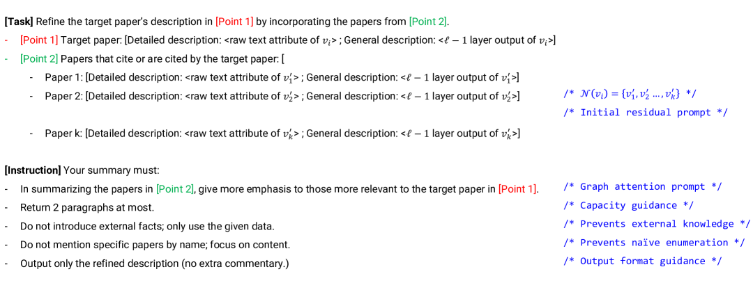
Figure 12: Example prompt of GLN for citation networks (oGBN-arXiv dataset).

Figure 13: Example prompt of GLN for co-purchase networks (Book-History dataset).

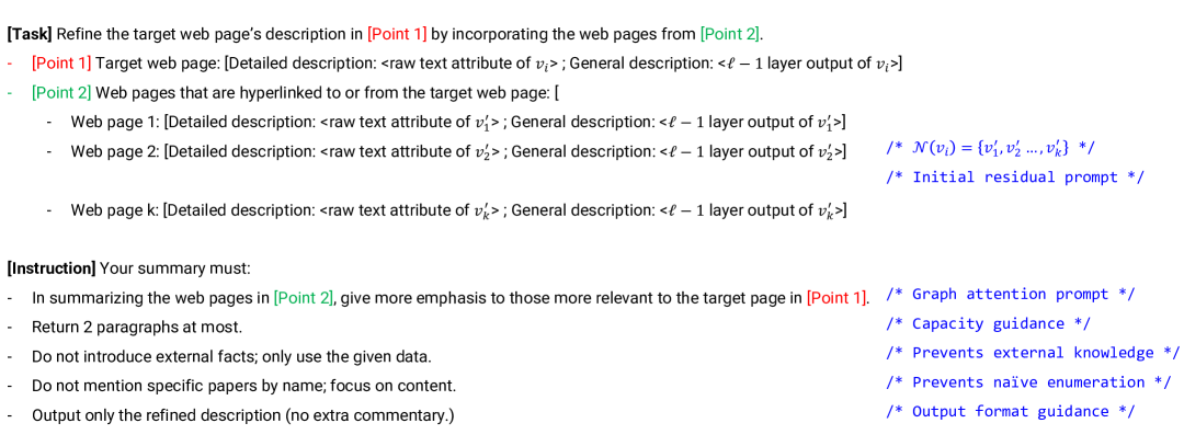
Figure 14: Example prompt of GLN for hyperlink networks (Wiki-CS dataset).

We provide a detailed prompt design of GLN. Specifically, we present the following prompts:

• Prompt for citation networks: A prompt for citation networks is in Figure 12.

• Prompt for co-purchase networks: A prompt for book co-purchase networks is in Figure 13.

• Prompt hyperlink networks: A prompt for hyperlink networks is in Figure 14.

D.2 Representation format of GLN

In this section, we further elaborate on the detailed format of the target node’s representation produced by GLN. Specifically, we present a format for a citation network.

Paper: {
- Detailed description: <initial text attribute>,
- General description: <layer-1 output of GLN >,
- Highly general description: <layer-2 output of GLN >} This format is provided as a representation for the target node (paper). In the co-purchase dataset (Book-History) and hyperlink dataset (Wiki-CS), we use the terms ‘Book’ and ‘Web page’, instead of Paper, respectively.

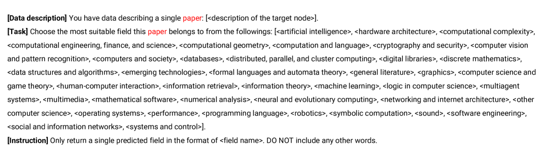
Figure 15: Example node classification prompt of GLN for citation networks (OGBN-arXiv dataset).

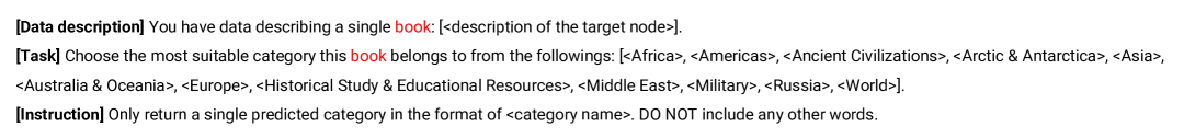
Figure 16: Example node classification prompt of GLN for co-purchase networks (Book-History dataset).

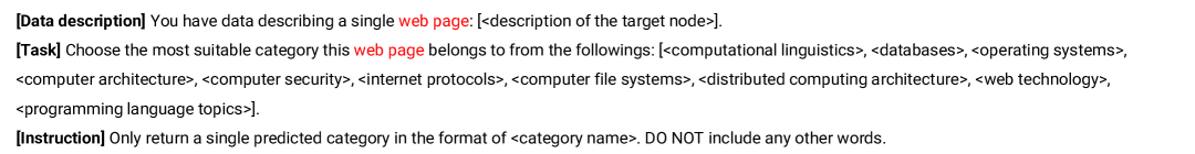
Figure 17: Example node classification prompt of GLN for hyperlink networks (Wiki-CS dataset).

D.3 Prompt for downstream tasks

In this section, we provide details regarding our prompt for downstream tasks, which are node classification and link prediction.

Node classification Example node classification prompts for the OGBN-arXiv dataset (citation network), Book-History (co-purchase), and Wiki-CS (hyperlink network), are provided in Figure 15, 16, and 17, respectively. Specifically, we provide a set of possible categories and ask the LLM to select the one the target node is most likely to belong to.

Link prediction Example link prediction prompts for the OGBN-arXiv dataset (citation network), Book-History (co-purchase), and Wiki-CS (hyperlink network), are provided in Figure 18, 19, and 20, respectively. Specifically, we present the LLM with four randomly sampled nodes and one ground-truth node, prompting it to select the node most likely to be linked to the target node. The prompt is tailored to reflect the semantics of the edge type. For example, in a co-purchase network, we ask: ‘Which book is most likely to be co-purchased with the target book?’.

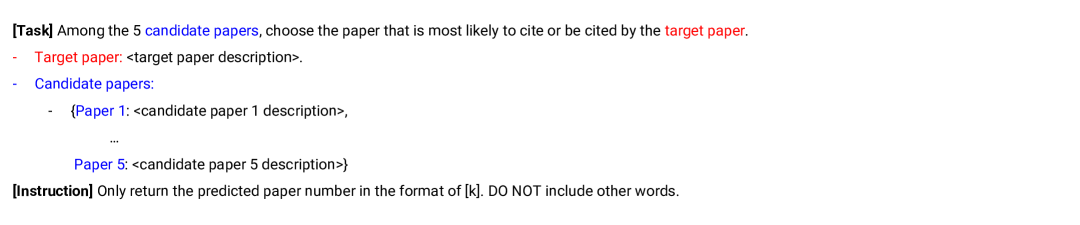
Figure 18: Example edge prediction prompt of GLN for citation networks (OGBN-arXiv dataset).

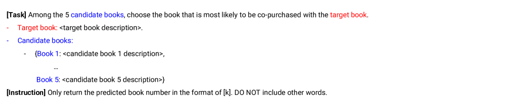
Figure 19: Example edge prediction prompt of GLN for co-purchase networks (Book-History dataset).

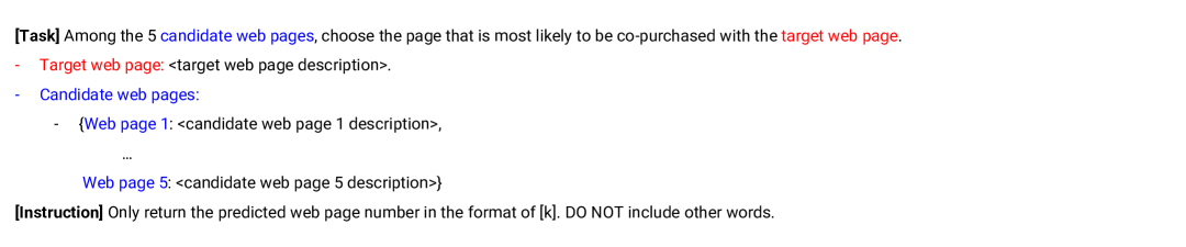
Figure 20: Example edge prediction prompt of GLN for hyperlink networks (Wiki-CS dataset).

Appendix E License and AI assistant usage

In this appendix section, we discuss (1) the licenses of the artifacts used in this work and (2) our use of an AI assistant, ChatGPT.

E.1 Licenses

The licenses of all artifacts used in this work are listed below:

• OGBN-arXiv dataset: ODC-BY (https://ogb.stanford.edu/docs/nodeprop/)

• Book-History dataset: MIT License (https://github.com/sktsherlock/TAG-Benchmark)

• Wiki-CS dataset: MIT License (https://github.com/pmernyei/wiki-cs-dataset)

• PromptGFM: CC-By-4.0 (https://arxiv.org/abs/2503.03313)

• GPT API: OpenAI permits academic use of the outputs generated by their models (https://openai.com/policies/).

• Claude API: Anthropic permits academic use of the outputs generated by their models (https://www.anthropic.com/legal/commercial-terms).

Note that all permits use for academic purposes.

E.2 AI Assistant usage

For this work, we used ChatGPT (Achiam et al., 2023) to assist with writing refinement and grammar checking.

References

- Achiam et al. (2023) Josh Achiam, Steven Adler, Sandhini Agarwal, Lama Ahmad, Ilge Akkaya, Florencia Leoni Aleman, Diogo Almeida, Janko Altenschmidt, Sam Altman, Shyamal Anadkat, and 1 others. 2023. Gpt-4 technical report. arXiv preprint arXiv:2303.08774.
- Cai et al. (2020) Han Cai, Chuang Gan, Tianzhe Wang, Zhekai Zhang, and Song Han. 2020. Once-for-all: Train one network and specialize it for efficient deployment. In ICLR.
- Chang et al. (2024) Yupeng Chang, Xu Wang, Jindong Wang, Yuan Wu, Linyi Yang, Kaijie Zhu, Hao Chen, Xiaoyuan Yi, Cunxiang Wang, Yidong Wang, and 1 others. 2024. A survey on evaluation of large language models. ACM transactions on intelligent systems and technology, 15(3):1–45.
- Chen et al. (2020) Ming Chen, Zhewei Wei, Zengfeng Huang, Bolin Ding, and Yaliang Li. 2020. Simple and deep graph convolutional networks. In ICML.
- Chen et al. (2024a) Runjin Chen, Tong Zhao, Ajay Jaiswal, Neil Shah, and Zhangyang Wang. 2024a. Llaga: Large language and graph assistant. In ICML.
- Chen et al. (2024b) Zhikai Chen, Haitao Mao, Hang Li, Wei Jin, Hongzhi Wen, Xiaochi Wei, Shuaiqiang Wang, Dawei Yin, Wenqi Fan, Hui Liu, and 1 others. 2024b. Exploring the potential of large language models (llms) in learning on graphs. ACM SIGKDD Explorations Newsletter, 25(2):42–61.
- Corso et al. (2024) Gabriele Corso, Hannes Stark, Stefanie Jegelka, Tommi Jaakkola, and Regina Barzilay. 2024. Graph neural networks. Nature Reviews Methods Primers, 4(1):17.
- Hamilton et al. (2017) Will Hamilton, Zhitao Ying, and Jure Leskovec. 2017. Inductive representation learning on large graphs. In NeurIPS.
- Hamilton (2020) William L Hamilton. 2020. Graph representation learning. Morgan & Claypool Publishers.
- He et al. (2024) Xiaoxin He, Xavier Bresson, Thomas Laurent, Adam Perold, Yann LeCun, and Bryan Hooi. 2024. Harnessing explanations: Llm-to-lm interpreter for enhanced text-attributed graph representation learning. In ICLR.
- Hu et al. (2020) Weihua Hu, Matthias Fey, Marinka Zitnik, Yuxiao Dong, Hongyu Ren, Bowen Liu, Michele Catasta, and Jure Leskovec. 2020. Open graph benchmark: Datasets for machine learning on graphs. In NeurIPS.
- Isola et al. (2017) Phillip Isola, Jun-Yan Zhu, Tinghui Zhou, and Alexei A Efros. 2017. Image-to-image translation with conditional adversarial networks. In CVPR.
- Keriven and Peyré (2019) Nicolas Keriven and Gabriel Peyré. 2019. Universal invariant and equivariant graph neural networks. In NeurIPS.
- Kipf and Welling (2017) Thomas N Kipf and Max Welling. 2017. Semi-supervised classification with graph convolutional networks. In ICLR.
- Luo et al. (2024) Yuankai Luo, Lei Shi, and Xiao-Ming Wu. 2024. Classic gnns are strong baselines: Reassessing gnns for node classification. In NeurIPS.
- Mernyei and Cangea (2020) Péter Mernyei and Cătălina Cangea. 2020. Wiki-cs: A wikipedia-based benchmark for graph neural networks. In ICML Workshop on graph representation learning and beyond.
- Peters et al. (2018) Matthew E Peters, Mark Neumann, Mohit Iyyer, Matt Gardner, Christopher Clark, Kenton Lee, and Luke Zettlemoyer. 2018. Deep contextualized word representations. In NAACL-HLT.
- Ren et al. (2024) Xubin Ren, Jiabin Tang, Dawei Yin, Nitesh Chawla, and Chao Huang. 2024. A survey of large language models for graphs. In KDD.
- Talak and Modiano (2020) Rajat Talak and Eytan H Modiano. 2020. Age-delay tradeoffs in queueing systems. IEEE Transactions on Information Theory, 67(3):1743–1758.
- Vaswani et al. (2017) Ashish Vaswani, Noam Shazeer, Niki Parmar, Jakob Uszkoreit, Llion Jones, Aidan N Gomez, Łukasz Kaiser, and Illia Polosukhin. 2017. Attention is all you need. In NeurIPS.
- Veličković et al. (2018) Petar Veličković, Guillem Cucurull, Arantxa Casanova, Adriana Romero, Pietro Lio, and Yoshua Bengio. 2018. Graph attention networks. In ICLR.
- Xu et al. (2019) Keyulu Xu, Weihua Hu, Jure Leskovec, and Stefanie Jegelka. 2019. How powerful are graph neural networks? In ICLR.
- Xu et al. (2018) Keyulu Xu, Chengtao Li, Yonglong Tian, Tomohiro Sonobe, Ken-ichi Kawarabayashi, and Stefanie Jegelka. 2018. Representation learning on graphs with jumping knowledge networks. In ICML.
- Yan et al. (2023) Hao Yan, Chaozhuo Li, Ruosong Long, Chao Yan, Jianan Zhao, Wenwen Zhuang, Jun Yin, Peiyan Zhang, Weihao Han, Hao Sun, and 1 others. 2023. A comprehensive study on text-attributed graphs: Benchmarking and rethinking. In NeurIPS.
- Zhu et al. (2025) Xi Zhu, Haochen Xue, Ziwei Zhao, Wujiang Xu, Jingyuan Huang, Minghao Guo, Qifan Wang, Kaixiong Zhou, and Yongfeng Zhang. 2025. Llm as gnn: Graph vocabulary learning for text-attributed graph foundation models. arXiv preprint arXiv:2503.03313.