LeDiFlow: Learned Distribution-guided
Flow Matching to Accelerate Image Generation

Abstract

Enhancing the efficiency of high-quality image generation using Diffusion Models (DMs) is a significant challenge due to the iterative nature of the process. Flow Matching (FM) is emerging as a powerful generative modeling paradigm based on a simulation-free training objective instead of a score-based one used in DMs. Typical FM approaches rely on a Gaussian distribution prior, which induces curved, conditional probability paths between the prior and target data distribution. These curved paths pose a challenge for the Ordinary Differential Equation (ODE) solver, requiring a large number of inference calls to the flow prediction network. To address this issue, we present Learned Distribution-guided Flow Matching (LeDiFlow), a novel scalable method for training FM-based image generation models using a better-suited prior distribution learned via a regression-based auxiliary model. By initializing the ODE solver with a prior closer to the target data distribution, LeDiFlow enables the learning of more computationally tractable probability paths. These paths directly translate to fewer solver steps needed for high-quality image generation at inference time. Our method utilizes a State-of-the-Art (SOTA) transformer architecture combined with latent space sampling and can be trained on a consumer workstation. We empirically demonstrate that LeDiFlow remarkably outperforms the respective FM baselines. For instance, when operating directly on pixels, our model accelerates inference by up to 3.75x compared to the corresponding pixel-space baseline. Simultaneously, our latent FM model enhances image quality on average by 1.32x in CLIP Maximum Mean Discrepancy (CMMD) metric against its respective baseline.

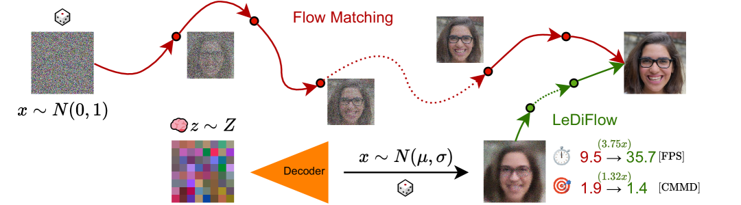
Figure 1: LeDiFlow produces an easier to solve transformation for flow matching-based generative modeling via a learned prior, enabling faster inference with higher image quality. $Z$ resembles the latent space.

1 Introduction

Generating high-quality and diverse images efficiently represents a central and ongoing challenge in Machine Learning (ML). DMs [14] have recently emerged as the SOTA for many image synthesis tasks, surpassing earlier approaches like Generative Adversarial Networks (GANs) [10] in terms of training stability and image quality. DMs use a diffusion process which gradually adds noise to the data in a forward process and during inference, use a noise prediction model to solve a Stochastic Differential Equation (SDE) initialized with pure random noise. This approach is used in SOTA text-to-image models, such as Stable Diffusion [29]. However, a significant operational drawback of DMs is their iterative generation process, which generally requires many steps and thus considerable computational resources for inference. To reduce the number of iterations, Adversarial Diffusion Distillation [31] copies principles from GANs by using a large diffusion teacher network to train a student model, which comes at the cost of multiple training runs. FM [23] presents a compelling alternative, offering advantages such as simulation-free training objectives compared to the score-based methods  [14, 18] typically used in DMs. Instead of an SDE, FM employs an ODE to define a transformation from a prior distribution $P\subseteq\mathbb{R}^{d}$ (e.g., a normalized Gaussian) to a target data distribution $Q\subseteq\mathbb{R}^{d}$ in data space $\mathbb{R}^{d}$. While promising, typical FM approaches that rely on a Gaussian prior generally induce a complicated to solve, time-dependent diffeomorphic map $\phi:[0,1]\times\mathbb{R}^{d}\rightarrow\mathbb{R}^{d}$ between $P$ and $Q$. A normalized Gaussian prior lacks specific structural information about the target data distribution, forcing the model to learn a complex, non-linear transformation to map noise to intricate image features. This transformation increases the computational complexity for any numerical ODE solver, necessitating many iterations and Neural Network (NN) inference calls to generate high-fidelity samples.

To reduce the complexity and enhance the efficiency of FM-based image generation, we propose LeDiFlow, a novel method to replace a Gaussian distribution with a learned prior distribution $P_{L}\subseteq\mathbb{R}^{d}$ via a regression-based auxiliary model (inspired by Variational Autoencoders (VAEs) [12, 19]). The core idea of LeDiFlow is a better-suited prior distribution $P_{L}$, which is learned by an auxiliary model, conditioned on a per-image latent vector, that maximizes the log-likelihood so that $P_{L}$ is as close to $Q$ as possible. Our method simplifies the complexity of the transformation $x\sim P_{L}\rightarrow y\sim Q$ that is induced by the Flow Matching Model (FMM), leading to fewer solver iterations required. The fundamental simplification of the transport problem directly translates into tangible benefits, like a reduction of the number of steps the ODE solver requires for high-quality image generation at inference time compared to standard FM approaches with a Gaussian prior.

Unlike methods, such as Rectified Flow [20, 25], which focuses on straightening learned paths through iterative refitting (Reflow), LeDiFlow simplifies the problem a priori by defining a more advantageous starting point for the ODE solver. Our approach utilizes a scalable transformer architecture [5, 7, 34], allowing for controllability through the latent space of the auxiliary model.

Our main contributions are:

• We propose LeDiFlow, a novel method for more efficient flow matching-based image generation by using an auxiliary prior-prediction model to reduce the complexity of the transformation between a source and target distribution.

• We introduce a variance-guided loss for training the prior-prediction model and adapt the FM loss with a prior based importance weighting scheme.

• We empirically demonstrate substantial improvements in inference speed and comparable or better image quality compared to the FM-baseline [23] on SOTA benchmark datasets (Flickr-Faces-HQ (FFHQ) [17], Landscapes High-Quality (LHQ) [32], Animal Faces-HQ (AFHQ) [3]) without requiring distillation or reflowing techniques.

2 Related Work

Early approaches to image generation focused on reconstructing images from compressed representations. Autoencoders (AEs) [13] learn an encoder to map an image to a low-dimensional latent space and a decoder to reconstruct the image, primarily aiming for dimensionality reduction [32]. VAEs [12, 19] extend this mapping by introducing a probabilistic latent space regularized using the Kullback-Leibler (KL) divergence between the learned latent distribution and a Gaussian prior [33]. The regularization encourages a continuous latent space suitable for generative sampling, and LeDiFlow adapts these principles for learning its informative prior distribution [34]. GANs [10, 33] improve image quality by replacing the pixel-wise reconstruction loss with an adversarial loss driven by a discriminator network. This method suffers from training instabilities such as mode collapse [24] or non-convergence [26] which makes GANs harder to train than DMs.

2.1 Flow Matching for Generative Modeling

FM [2, 23, 25] offers a distinct paradigm for generative modeling. For a given prior distribution $P\subseteq\mathbb{R}^{d}$ and target data distribution $Q\subseteq\mathbb{R}^{d}$ in data space $\mathbb{R}^{d}$, FM formulates a time-dependent vector field $v:[0,1]\times\mathbb{R}^{d}\rightarrow\mathbb{R}^{d}$ that dictates the transformation of samples $x\sim P\rightarrow y\sim Q$. The transformation is called a time-dependent, diffeomorphic map $\phi:[0,1]\times\mathbb{R}^{d}\rightarrow\mathbb{R}^{d}$ and can be written as an ODE:

$$\frac{d}{dt}\phi_{t}(x) =v_{t}(\phi_{t}(x))$$ (1)

$$\phi_{0}(x) =x$$

$$y =\phi_{0}(x)+\int_{0}^{1}v_{t}(\phi_{t}(x))dt,$$

with $v_{t}(\phi_{t}(x))$ being the unknown vector value of $x$ at time $t\in[0,1]$. We define $T=1$ with $\phi_{T}(x)=y$ as the end-state of the transformation. This formulation is shown to be easier to solve than the score-based SDE used in DMs [23, 25]. The solution to Equation˜1 is given by an ODE solver, which needs to access the high-dimensional vector field $v$. [2] proposes using a NN to model the vector field. From now on, we call the network parameters $\theta$ and $f(x;\theta)$ the result when using these parameters for computation of a function $f$. The FMM is called $\theta_{\mathrm{FM}}$ and is conditioned on the current timestep $t$ and $\phi_{t}(x)\in\mathbb{R}^{d}$. To train $\theta_{\mathrm{FM}}$, a simulation-free training objective is employed. This objective is considered ’simulation-free’ as it directly regresses the target vector field from pairs of prior samples and corresponding data points, without requiring iterative simulation of a diffusion or denoising process during training. We use the rectified flow objective [25], which sets $\sigma_{\mathrm{min}}=0$ from [23] and can be written as:

$$\mathcal{L}_{\mathrm{CFM}}(\theta_{\mathrm{FM}})=\|v_{t}(\phi_{t}(x);\theta_{\mathrm{FM}})-(y-x)\|^{2}\\ ,$$ (2)

where $\|x\|$ represents the Euclidean norm. Despite the linear training objective, the vector field $v$ induced by $\theta_{\mathrm{FM}}$ typically leads to a complex transformation $\phi$, that needs many iterations for accurately solving Equation˜1. During training, following standard FM practices [23], a random timestep $t\in[0,1]$ is sampled and a point $\phi_{t}(x)=yt+x(1-t)$ is calculated by linearly interpolating between sample $x\sim P$ and $y\sim Q$. This interpolation already defines the objective of $\theta_{\mathrm{FM}}$, learning a vector field with direct paths from $x\rightarrow y$.

2.2 Architectures and Conditional Control

The performance of generative models heavily depends on the underlying network architecture. While early diffusion-based models use U-Net [18, 28, 30] style architectures, transformers [7, 34] are effective in image-related tasks. The Diffusion Transformer (DiT) [22] adapts properties from the Vision Transformer [7] for use in DMs. Hourglass Diffusion Transformer (HDiT) [5] joins the hierarchical nature of U-Nets with the transformer backbone of DiT, achieving better computational efficiency when scaling to higher image resolutions. To improve the training time, Latent Diffusion Models (LDMs) [9, 29] generates images in a smaller latent space, which then gets upsampled to a high-resolution RGB image. The latent space is induced by a Vector Quantized Generative Adversarial Network (VQ-GAN) [8, 33], which has been shown to have minimal impact on image quality whilst drastically reducing the image resolution and speeding up the training time of DMs. LeDiFlow builds upon these advancements, utilizing a transformer-based architecture similar to HDiT [5] for both its auxiliary prior prediction and the main FMM.

Beyond unconditional generation, controlling the output is crucial for many applications. ControlNet [35] demonstrates the addition of fine-grained spatial conditioning (e.g., edges, pose) to pre-trained text-to-image DMs. Diffusion Autoencoders [28] combine DMs with autoencoding principles to learn meaningful and traversable latent representations, enabling applications such as facial feature editing and manipulation. The latent space used by the auxiliary model of LeDiFlow also offers controllability, allowing for applications such as image interpolation, face anonymization [15, 36] and conditional generation.

3 LeDiFlow Architecture

The standard FM process typically uses a normalized Gaussian prior $P_{N}=\mathcal{N}(0,1)\subseteq\mathbb{R}^{d}$ and a target data distribution $Q$. As mentioned earlier, training with $P_{N}$ induces a highly curved vector field $v$ learned by a FMM $\theta_{\mathrm{FM}}$. To reduce the number of steps of the ODE solver, we propose to use a learned prior $P_{L}\subseteq\mathbb{R}^{d}$. The prior is given by an auxiliary model that is trained to predict $P_{L}$ as close to $Q$ as possible making the traversed vector field of the transformation computationally more tractable.

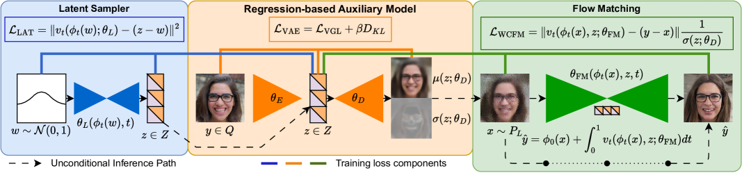
Figure 2: LeDiFlow Pipeline. An auxiliary model (middle) maps images $y\sim Q$ into latent vectors $z\sim Z$, from which the decoder defines a learned prior $P_{L}=\mathcal{N}(\mu(z;\theta_{D}),\sigma^{2}(z;\theta_{D}))$. In latent space (left), we train a flow model $\theta_{L}$ to match trajectories from Gaussian noise $w\sim\mathcal{N}(0,1)$ to semantic codes $z$, using supervised vectors $z-w$. In image space (right), another flow model $\theta_{\mathrm{FM}}$ transforms samples $x\sim P_{L}$ into the data distribution via flow matching towards $y\sim Q$. Dashed lines denote forward inference, solid lines are training-time supervision.

In Figure˜2, we give an overview of the LeDiFlow architecture. The training is done with three modules. First, we train an auxiliary model consisting of an encoder $\theta_{E}$ and decoder $\theta_{D}$ with the goal of obtaining a continuous latent space $Z$ and the learned prior distribution $P_{L}$. We define the $Z$ having a dimension of $k=256$ shaped like an image of $8\times 8\times 4$ pixels. Secondly, we train the FMM $\theta_{\mathrm{FM}}$ conditioned on the pretrained latent space $Z$ and stochastic samples $x\sim P_{L}$. Last, we train a latent sampler $\theta_{L}$ that is used to transform a Gaussian normal distribution $N(0,1)\subseteq\mathbb{R}^{k}\rightarrow Z$ using traditional FM. For image generation, we transform a sample $w\rightarrow z\in Z$, use $\theta_{D}$ to decode the latent vector into a per pixel distribution $P_{L}(z)=\mathcal{N}(\mu(z;\theta_{D}),\sigma(z;\theta_{D}))$ and draw a sample $x\sim P_{L}$. $x$ is then used by an ODE solver, which calls the FMM $\theta_{\mathrm{FM}}$ conditioned on $z$ and $\phi_{t}(x)$ multiple times, to obtain a high-quality image $\hat{y}\in Q$. Variation is induced by the sampling process of $P_{L}$ and thus, a constant latent vector $z$ produces contextually similar, but visually different, results. The auxiliary model and FMM share a similar architecture based on the HDiT [5]. The hierarchical architecture allows training on hardware with lower performance by using neighborhood attention layers instead of global ones. All models are trained individually while $\theta_{\mathrm{FM}}$ and $\theta_{L}$ require the auxiliary model to be pretrained.

3.1 Regression-based Auxiliary Model (Distribution Prediction)

The first module of our architecture is the auxiliary model (middle block in Figure˜2), which consists of the encoder $\theta_{E}$ and the decoder $\theta_{D}$. This model has two goals: The training defines the continuous latent space $Z$ where every image $y\in Q$ is mapped to a latent vector $z\sim\mathcal{N}(\mu(y;\theta_{E}),\sigma^{2}(y;\theta_{E}))$ using the Bayesian mapping of the auxiliary model. The second goal is training the decoder to predict the prior distribution $P_{L}$ to sample from for use in the FM process. The perfect distribution would be as close to $Q$ as possible. As getting an exact solution is very challenging to do using regression training, the decoder predicts a tuple of values for every pixel, namely the mean $\mu(z;\theta_{D})$ and the log variance $\log\sigma^{2}(z;\theta_{D})$. We then define the goal as to optimize $\mu(z;\theta_{D})$ and $\sigma^{2}(z;\theta_{D})$ so that the probability of a pixel sample $y\in Q$ is as high as possible, giving a Gaussian normal distribution $\mathcal{N}(\mu(z;\theta_{D}),\sigma^{2}(z;\theta_{D}))$:

$$\mathcal{N}(y|\mu(z;\theta_{D}),\sigma^{2}(z;\theta_{D}))=\frac{1}{\sqrt{2\pi\sigma^{2}(z;\theta_{D})}}e^{-\frac{(y-\mu(z;\theta_{D}))^{2}}{2\sigma^{2}(z;\theta_{D})}}.$$ (3)

Optimizing the Gaussian distribution is complicated as the optimization target function is flat far away from the optimum, which leads to vanishing gradients at large $|y-\mu(z;\theta_{D})|$. For this reason, we optimize $\log\mathcal{N}(\mu(z;\theta_{D}),\sigma^{2}(z;\theta_{D}))$, which has the same minimum as the normal distribution itself. This process is similar to the optimization of the log-likelihood function [4]. We call our loss the Variance Guided Loss (VGL):

$$\mathcal{L}_{\text{VGL}}(y|\mu(z;\theta_{D})),\sigma(z;\theta_{D})) =-\log\mathcal{N}(y|\mu(z;\theta_{D}),\sigma(z;\theta_{D}))$$ (4)

$$=\frac{1}{2}\left(\frac{(y-\mu(z;\theta_{D}))^{2}}{\sigma^{2}(z;\theta_{D})}+\log\sigma^{2}(z;\theta_{D})+\log(2\pi)\right).$$

During training, the log-variance $\log\left(\sigma^{2}(z;\theta_{D})\right)$ is predicted by the NN. The decoder parameters $\mu(z;\theta_{D})$ and $\sigma(z;\theta_{D})$ define a learned prior distribution $P_{L}=\mathcal{N}(\mu(z;\theta_{D}),\sigma(z,\theta_{D}))$, from which we draw initial image samples $x\sim P_{L}$. These serve as the starting point for the FM process. We then combine the reconstruction and KL loss the following way:

$$\mathcal{L}_{\mathrm{VAE}}(\theta_{E},\theta_{D})=\beta D_{KL}(Z||\mathcal{N}(0,1);\theta_{E})+\mathcal{L}_{\mathrm{VGL}}(\theta_{D}),$$ (5)

where $\beta$ is a user controlled parameter [12]. A lower $\beta$ leads to better reconstruction but a worse feature mapping in latent space. We found $\beta=10^{-3}$ to be a good fit.

3.2 Flow Matching

The second module of our architecture is the FMM $\theta_{\text{FM}}$ used by the ODE solver for transporting samples $x\sim P_{L}$ to image values $y\sim Q$. The FMM is based on an HDiT [5] and consists of multiple neighborhood and global attention layers, down- / upsample layers and skip connections. We train the model by decoding images $y\in Q$ from the dataset using $\theta_{E}$ into a latent representation $z=(\mu(y;\theta_{E}),\sigma(y;\theta_{E}))\in Z$ and an initial image distribution $P_{L}$. We then sample $\hat{z}\sim\mathcal{N}(\mu(y;\theta_{E}),\sigma^{2}(y;\theta_{E}))$ and $x\sim P_{L}$. The model $\theta_{\text{FM}}$ is then conditioned on $\hat{z}$ and a random timestep $t\in[0,1]$ is used for the training sample $\phi_{t}(x)$. The FM training is then done similar to the standard flow matching procedure [23] with one key difference in our approach being the introduction of an importance scaling term, $\frac{1}{\sigma(z;\theta_{D})}$, applied per pixel to the squared error in the loss function. Here, $\sigma(z;\theta_{D})$ represents the standard deviation of our learned prior distribution $P_{L}$. This weighting strategy serves a dual purpose:

1. Refining confident predictions: For pixels where $\mu(z;\theta_{D})$ is confident (i.e., $\sigma(z;\theta_{D})$ is small), the term $\frac{1}{\sigma(z;\theta_{D})}$ becomes large, which up-weights the loss for these pixels. The weighting encourages $\theta_{\mathrm{FM}}$ to learn very precise adjustments effectively refining the already strong predictions from $\theta_{D}$. Dividing by $\sigma(z;\theta_{D})$ can generate large weight values, which we prevent by clipping the divider to a maximum value of $10^{-3}$. This way, bad pixels with a very large weight do not add to the loss relative to the rest of the image pixels and batch.

2. Stabilizing learning for uncertain predictions: Conversely, for pixels where the prior is uncertain (i.e., $\sigma(z;\theta_{D})$ is large), the loss contribution is down-weighted, which prevents noisy pixels (i.e. difficult to estimate) from dominating the training signal of $\theta_{\mathrm{FM}}$, potentially leading to a more stable vector field $v$.

The importance-weighted loss is given by:

$$\mathcal{L}_{\mathrm{WCFM}}(\theta_{\mathrm{FM}})=\|v_{t}(\phi_{t}(x),\hat{z};\theta_{\mathrm{FM}})-(y-x)\|^{2}\frac{1}{\sigma(z;\theta_{D})}.$$ (6)

3.3 Latent Sampling

To generate new randomized data samples $\hat{y}\in Q$, we need to be able to sample the latent space $Z$. As we use the KL-Divergence for regularization, the latent space learned by our auxiliary model should be continuous. To sample $z\sim Z$, we need to either do a Principal Component Analysis (PCA) [27] or transform from an easier-to-sample distribution to the latent one. As PCA does not work well for arbitrary distributions, we opted for the second solution, also used similarly in diffusion autoencoders [28]. Our latent space $Z$ has the shape $8\times 8\times 4$ and we can treat it like an image with four channels. We then use a FMM $\theta_{L}$, which is built on a simplified HDiT architecture, and the standard FM training method from Section˜2.1. The loss from Equation˜2 is used to transform a normalized Gaussian distribution $P_{N}\rightarrow Z$. The latent sampler is placed on the left in Figure˜2 and uses the latent encodings $z\in Z$ calculated by the pretrained encoder model $\theta_{E}$ for its training loop.

4 Results

In this section, we show results using models trained on a consumer workstation (Intel Core i7-10700K, 64GB RAM, two NVIDIA RTX 3090) and a server (76 CPU cores, four NVIDIA A100 40GB GPUs). The server handles the more compute and memory intensive models for operation in RGB pixel space explained in [5]. The workstation handled training with pre-encoded images using the pretrained Stable Diffusion 2 VAE (SDV). This encoder compresses RGB images into a latent space representation with an image size reduction of 8 whilst increasing the channel count to 4. Thus, images with the size of $256^{2}\times 3$ are compressed into an image with size $32^{2}\times 4$. All models were trained in approximately 3̃0h. We compare our method to the reference FM implementation using the same HDiT architecture in unconditional and conditional generation tasks. We evaluate our findings using the FFHQ, AFHQ, LHQ and ImageNet datasets.

4.1 Unconditional Generation

Table 1: Performance and quality comparison of the HDiT-S/4 [5] architecture using the standard FM [23] algorithm and the method proposed in this work using different datasets at $\boldsymbol{256^{2}}$ resolution. The performance is measured on an RTX 4070 Super with batch size 64. FM uses 8 inference steps while LeDiFlow uses 4 latent + 2 FM steps for the Midpoint method and 2 + 1 steps for the 3rd-order Heun method (Heun3 [1]). $\dagger$ The decoding cost using the SDV decoder is $\approx 20\mathrm{ms}$ per image.

Method	FM	LeDiFlow	FM (SDV)	LeDiFlow (SDV)
# Parameters	160M	213M	154M	207M
Evaluation (CMMD) $\downarrow$
FFHQ [17]	2.48	2.66	2.00	1.08
AFHQ [32]	1.08	1.33	0.81	0.87
LHQ [3]	1.55	1.39	1.48	1.21
ImageNet [6]	-	-	3.10	2.45
Inf. time [ms/img] $\downarrow$
Midpoint	105	32	80†	40†
Heun3 [1]	116	28	85†	37†

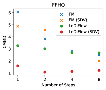
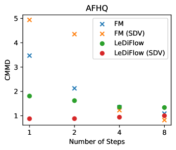
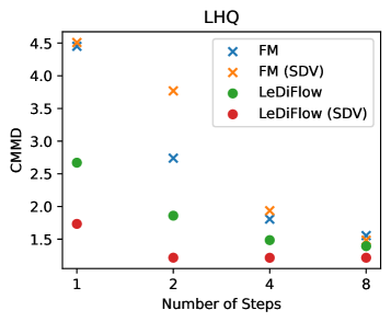
Figure 3: Visual scatter plot showing the comparison from Table˜1.

In Table˜1 and Figure˜3, we compare the methods in quality and inference time. The quality is assessed using the CMMD [16] metric. CMMD was chosen because it is a more recent image quality metric and more stable compared to the Frechet Inception Distance (FID) [11]. The results show that our method achieves speed improvements in inference while maintaining competitive or superior image quality. The scatter plots in Figure˜3 show that our method converges faster and produces comparable results with only one step of flow matching using an ODE solver of 2nd order or higher (i.e. midpoint, Heun). With LeDiFlow using an auxiliary prior prediction model, the cost of initializing the ODE solver is higher compared to using $P_{N}$. Despite this cost, our method up to 3.75x faster than the default FM method, as LeDiFlow needs less steps to achieve the same image quality. Latent sampling uses 4 steps and the midpoint solver, which takes $\approx 5\mathrm{ms}$ whilst the decoder $\theta_{D}$ takes $\approx 3\mathrm{ms}$. The reason inference in pixel space (RGB) is faster compared to the SDV compressed image is the high decoding and inference cost of the SDV decoder model ($\approx 20\frac{\mathrm{ms}}{\mathrm{img}}$). The tests are done using unconditional samples for all models and Figure˜4 visualizes 32 random images produced with our method from each dataset.

An interesting phenomenon occurs with LeDiFlow (SDV) that the CMMD score does not decrease with more steps. We have also seen this behavior using the 3rd order Heun method and examined a set of images with deterministic seeding (see Appendix). The images look visually very similar and only differ in minor details, which get picked up by the CMMD metric [16]. Findings on ODE dynamics [18, 21] describe, how small errors in the vector field prediction can accumulate to a worse result.

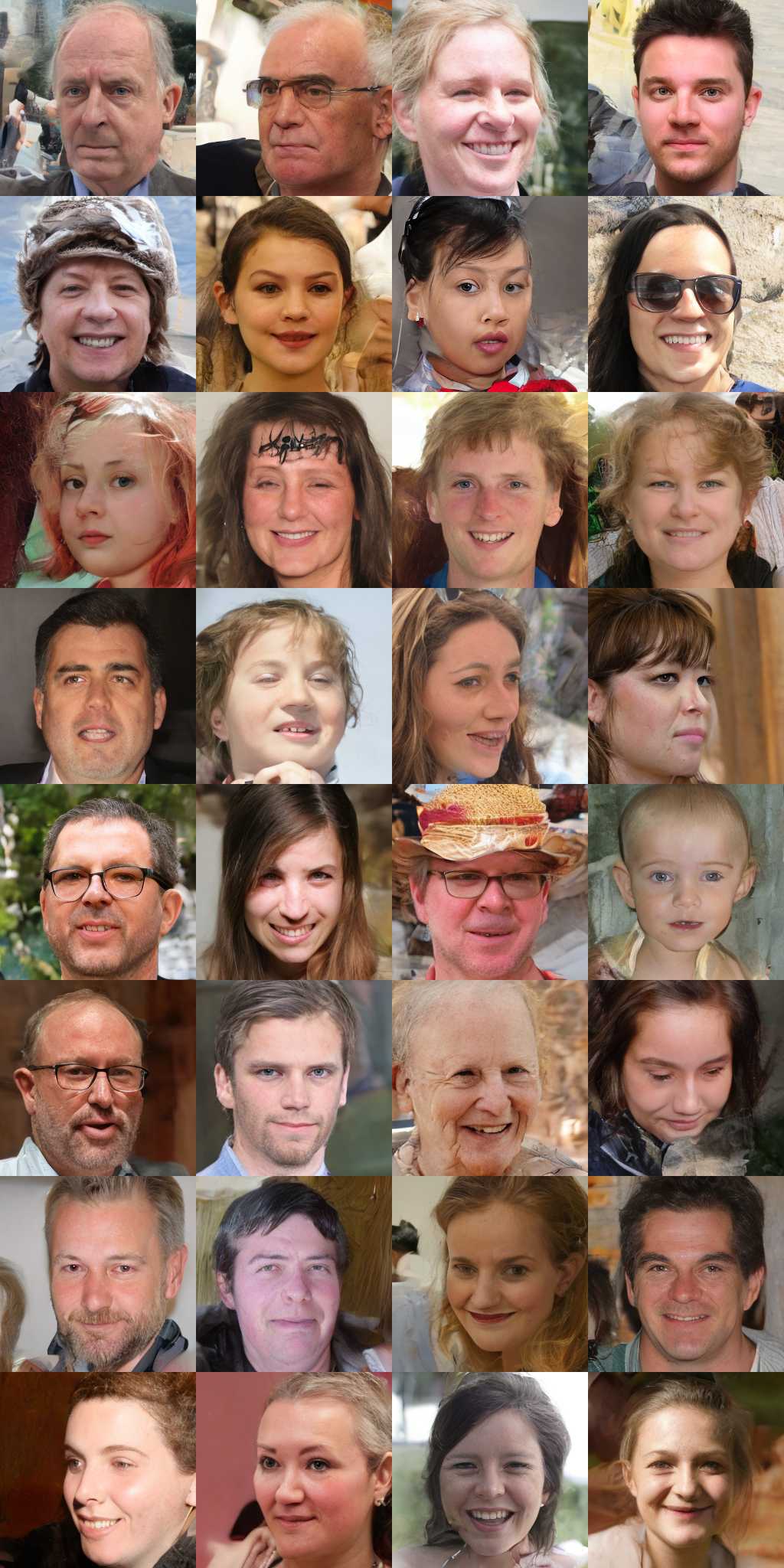
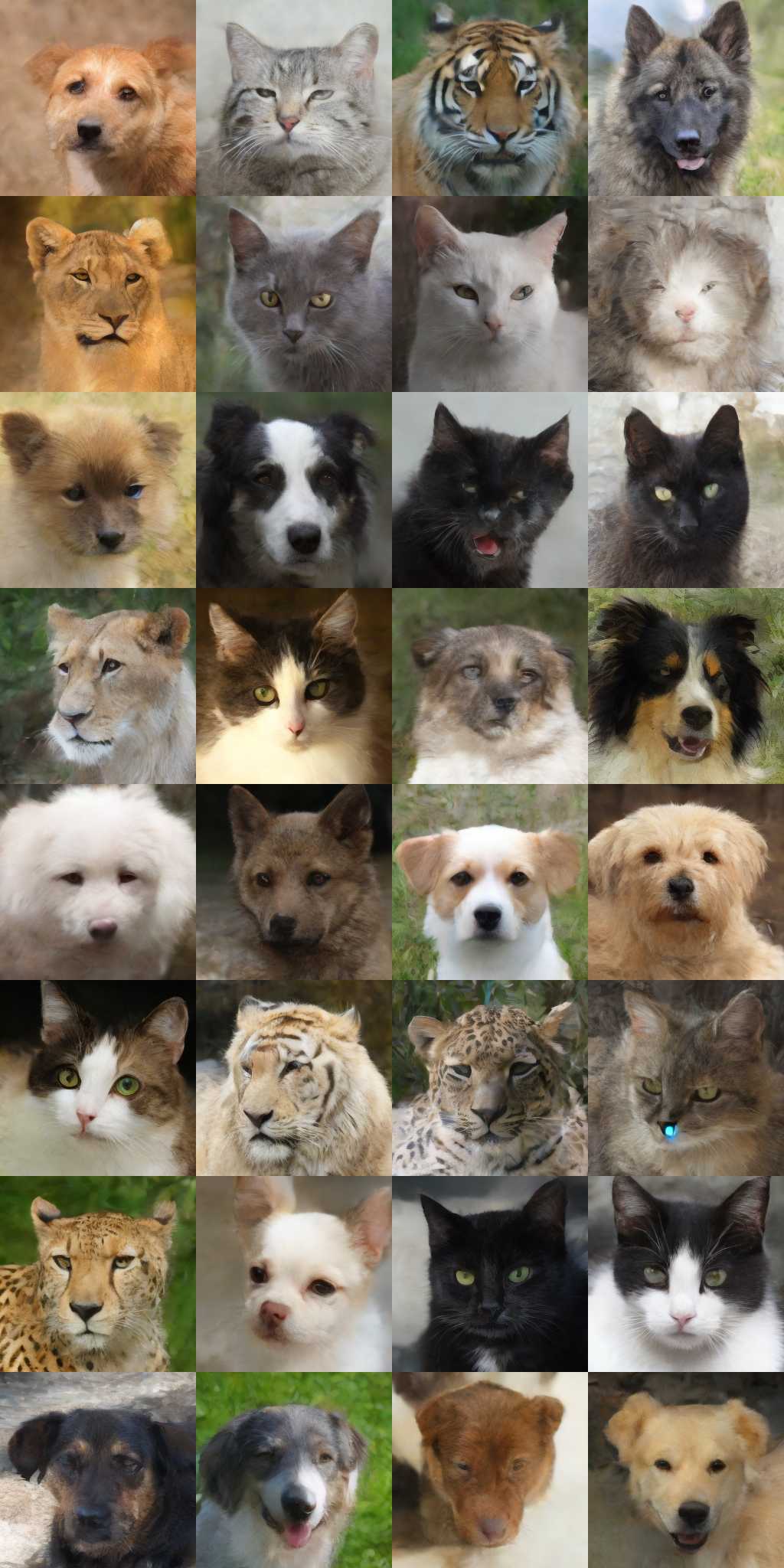
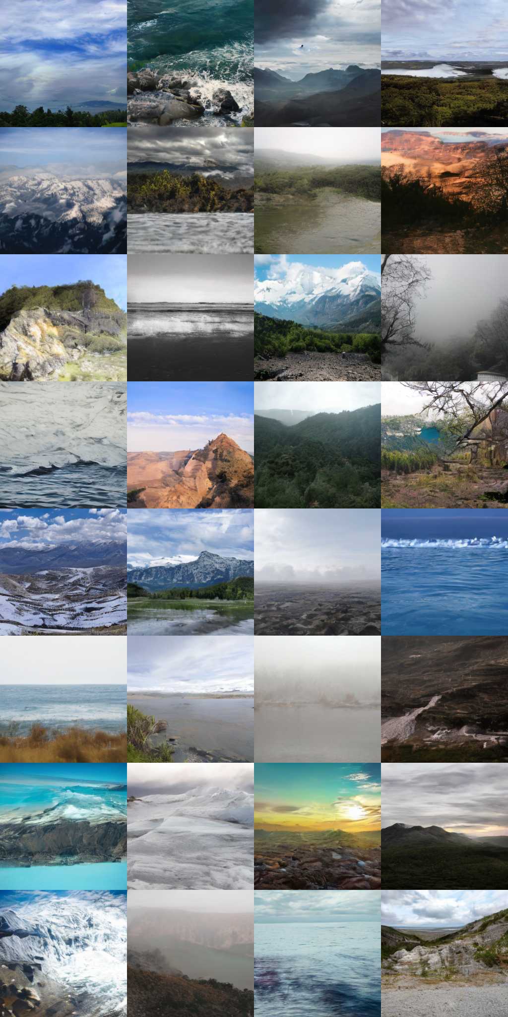
Figure 4: Samples showing unconditional generation of our method using 4 inference steps (Midpoint solver). From left to right: FFHQ [17], AFHQ [32], LHQ [3]

4.2 Conditional Applications

In this section, we look at applications of our method when modifying the latent space vector $z$. We start with a popular application when using VAEs, interpolating between points in latent space. In contrast to normal VAEs, we have two possibilities of doing the interpolation, linear in $Z$ or linear in $\mathcal{N}(0,1)$ using $\theta_{L}$ for the transformation.

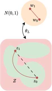
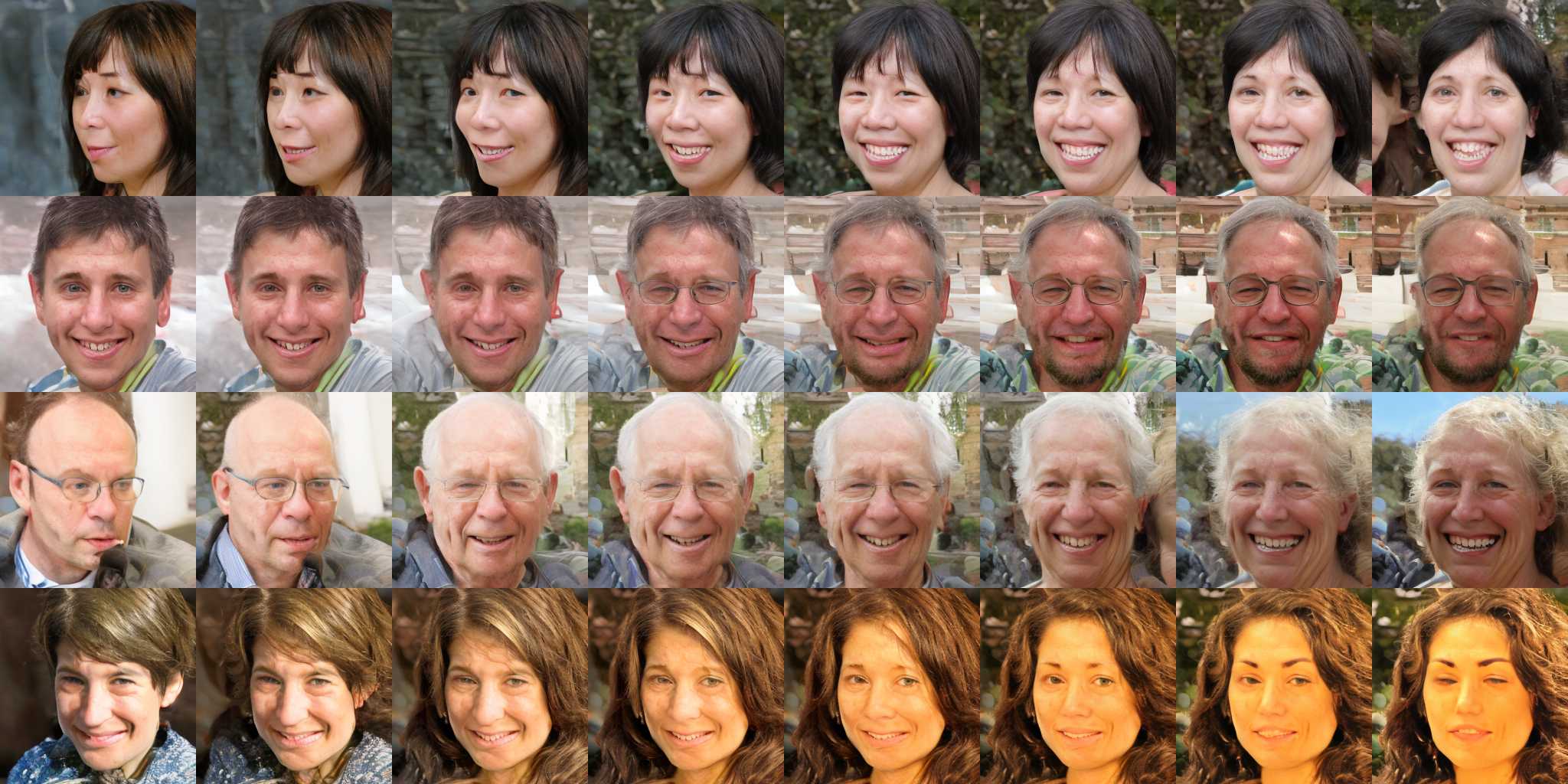
Figure 5: (Left) Visualization of the interpolation of samples $w\in\mathcal{N}(0,1)$ that are transformed into valid samples $z\in Z$ using $\theta_{L}$. (Right) Generated images from random latent vectors $z_{0}$ on the left and $z_{1}$ on the right using a constant noise seed.

In Figure˜5 on the left, we see problems that can occur when using the first approach. We do not know the high-dimensional shape of $Z$ and where most of the data is located. The shape might be nonconvex, thus, interpolating linearly can cross sparse or empty regions. To avoid these regions, we use method two and linearly interpolate in $\mathcal{N}(0,1)$ between two reverse-mapped vectors $w_{0}$ and $w_{1}$ given by reverse flow matching using $\theta_{L}$. The interpolated value is then mapped back to $Z$ using the latent sampler $\theta_{L}$ from Section˜3.3, which results in a non-linear interpolation between $z_{0}$ and $z_{1}$. Looking at image samples on the right, we see that in all cases, the interpolated image contains valid data although with varying quality.

Another popular example is image inpainting. We show this task briefly in Figure˜6 where the input image $y$ (left) is passed through the full auxiliary model pipeline to get a latent vector $z$ and an initial noisy image $x\sim P_{L}$. We also provide a mask $m$ indicating where the FMM should generate pixels. The generation is already given by the general FM formulation. The vector prediction of $\theta_{\mathrm{FM}}$ is used to calculate the flow of missing pixels provided by $m$. The modified vector field $\hat{v}:[0,1]\times\mathbb{R}^{d}\rightarrow\mathbb{R}^{d}$ for inpainting is given by:

$$\hat{v}_{t}(\phi_{t}(x)) =\begin{cases}v_{t}(\phi_{t}(x);\theta_{\mathrm{FM}})&\text{where }m==1\\ y-x&\text{else}\end{cases}.$$ (7)

Using this equation, the flow matching process is forced to move in a straight line for every non-masked pixel towards $y$.

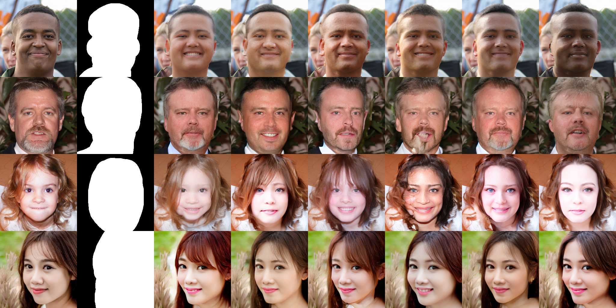
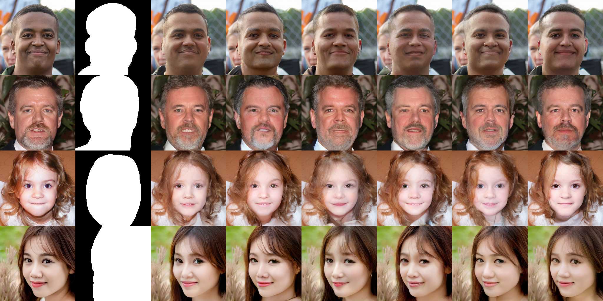
Figure 6: Our method is used to inpaint the original image (1st column) using a binary mask (2nd column). On the left half, we vary the latent space vector $z$ with a constant noise seed for drawing $x\sim P_{L}$ and on the right half, $z$ is constant and we vary the seed for drawing $x\sim P_{L}$.

On the left half in Figure˜6, we mapped $z\xrightarrow{\theta_{L}}w\in\mathcal{N}(0,1)$ using $\theta_{L}$ and reverse ODE solving and added a small random vector $r\in\mathcal{N}(0,1)$ to $w$ and then transformed it back using $w+\alpha r\xrightarrow{\theta_{L}}\hat{z}$ with $\alpha=0.5$. This alters the latent vector and, consequently, the identity of the face slightly. We see that all non-masked areas do not change compared to the original image, whilst the masked areas are seamlessly inpainted using our method. On the right half, we see that changing the noise with a constant vector $z$ results in small details changing, while the overall face style is preserved.

More results and comparisons (i.e. plots, images, FID values) are provided in the Appendix.

5 Limitations and Broader Impacts

First, our method is highly dependent on the quality of the learned prior. A bad prior might be worse than using a Gaussian prior, as the transformation map might be more complex. Second, while LeDiFlow demonstrates effectiveness on domain-specific datasets like FFHQ, AFHQ, LHQ the current model configuration (based on the HDiT S/4 backbone) struggles with the complexity and diversity of large-scale datasets such as ImageNet [6]. Preliminary experiments indicated that neither LeDiFlow nor the baseline FM achieves satisfactory performance on ImageNet at this scale, suggesting that significant architecture scaling or adaptation is required for such challenging domains. Third, a bad variance prediction $\sigma(z;\theta_{D})\approx 0$ can lead to a mostly discrete prior, which is challenging to use for FM. Fourth and finally, this paper has only shown a single model architecture, which is used in all three of the presented steps LeDiFlow needs to generate an image. Optimized architectures for the different steps can lead to better performance overall.

LeDiFlows efficiency improvements can enhance accessibility to creative tools and support research, for example, through synthetic data generation or applications like face anonymization demonstrated in this work. However, advancements in realistic image synthesis also pose risks, such as potential misuse for disinformation and the amplification of data biases (e.g., from FFHQ, AFHQ datasets). Continued research into content detection and bias mitigation remains crucial for responsible development. To promote responsible use of our contributions, our released code will be available under an MIT license. Pretrained models will be accompanied by Model Cards detailing their capabilities, limitations, ethical considerations, and data sources.

6 Conclusion and Future Work

This work presents LeDiFlow, a scalable method that utilizes a learned prior distribution to enhance the inference performance of flow matching models. Instead of relying on a static Gaussian distribution as the prior, LeDiFlow uses a learned distribution for the initial step of the FM algorithm. This approach reduces computational requirements, needing only half to one-third of the inference time compared to baseline FM, while achieving competitive, or superior image quality, particularly on datasets like FFHQ (SDV) and LHQ. We prove the capabilities of LeDiFlow by evaluating unconditional generation capabilities on multiple datasets and comparing against the reference FM implementation. Our work primarily targets smaller models for specific use cases that involve images with a similar context, such as faces [17], animals [32] or landscapes [3]. Additionally, we also examine image inpainting and latent space interpolation, two popular applications of image generation models showing promising results. Future work could focus on applying different architectures on the components from LeDiFlow to improve the quality while maintaining affordable inference time. A potential future application of full-text-to-image generation would also be an interesting test case. This could demonstrate the general scalability of LeDiFlow and how the prediction of the prior responds to a more diverse dataset comprising various scenes.

Appendix

Symbol	Description
$P$	Source distribution
$P_{L}$	Learned prior distribution
$P_{N}$	Gaussian normal distribution $\mathcal{N}(0,1)$
$Q$	Target distribution (i.e. images)
$Z$	Latent space distribution induced by the VAE model
$x\sim P$	Source sample from $P$
$y\sim Q$	Target sample from $Q$
$t\in[0,1]$	Timestep
$v_{t}(\phi_{t}(x))$	Learned vector field for sample $x$ time-dependent on $t$
$v_{t}(\phi_{t}(x);\theta)$	Learned vector field for sample $x$ time-dependent on $t$ using the neural network $\theta$
$\phi_{t}(x)$	Transformation state at timestep $t$ when initialized with $x$
$\hat{y}$	Result after solving the flow matching integral $\hat{y}=\phi_{0}(x)+\int_{0}^{1}v_{t}(\phi_{t}(x))dt$
$z\in Z$	Latent vector for an image sample $y$
$\mu(y;\theta_{D})$	Mean of a latent variable
$\sigma(y;\theta_{D})$	Standard deviation of a latent variable
$\mu(z;\theta_{E})$	Mean of the a prior variable inducing $P_{L}$
$\sigma(z;\theta_{E})$	Standard deviation of the a prior variable inducing $P_{L}$
$\theta_{\mathrm{FM}}$	Flow matching model
$\theta_{E}$	VAE Encoder model
$\theta_{D}$	VAE Decoder model
$\theta_{L}$	Latent sampling model

Table 2: Math symbols used in the paper

Table 3: Parameters used for our different models

Image Type	RGB	SDV
Resolution	$256^{2}$	$32^{2}$
Flow Matching Model
# Parameters	160M	154M
Patch Size	4	1
Levels (Local + Global Attention)	2 + 1	1 + 1
Depth	[2, 2, 8]	[2, 8]
Widths	[256, 512, 1024]	[512, 1024]
Attention Head Dim	64	64
Mapping Depth	2	2
Mapping Width	768	768
Neighborhood Kernel Size	7	7
Batch Size	128	64
Auxiliary model
# Parameters	37M	35M
Levels (Local + Global Attention)	4 + 1	3 + 1
Depth	[2, 2, 2, 2, 2]	[2, 2, 2, 2]
Widths	[128, 256, 512, 512]	[256, 512, 512]
Attention Head Dim	16	16
Latent Shape	$8\times 8\times 4$	$8\times 8\times 4$
Neighborhood Kernel Size	7	7
Batch Size	256	128
Latent Sampler
# Parameters	17M	17M
Levels (Global Attention)	1	1
Depth	[8]	[8]
Widths	[384]	[384]
Attention Head Dim	64	64
Batch Size	512	256
Training Settings
Optimizer	AdamW	AdamW
Betas	(0.9, 0.99)	(0.9, 0.99)
Learning Rate	3e-4	3e-4
Precision	bfloat16	bfloat16

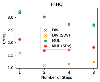
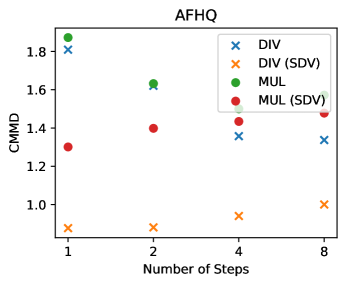
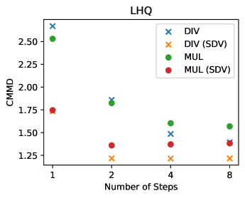
Figure 7: Comparison of using multiplication vs division importance scaling in Equation˜6.

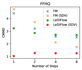
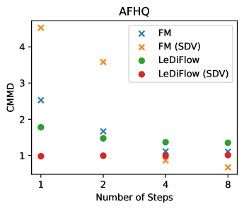
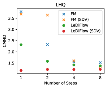
Figure 8: Comparison of FM and LeDiFlow similar to Figure˜3.

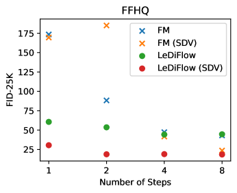
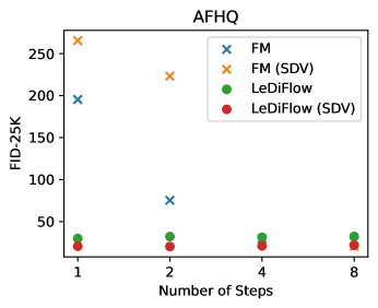
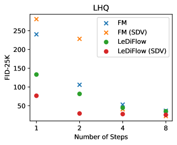
Figure 9: FID values comparing FM with LeDiFlow similar to Figure˜3.

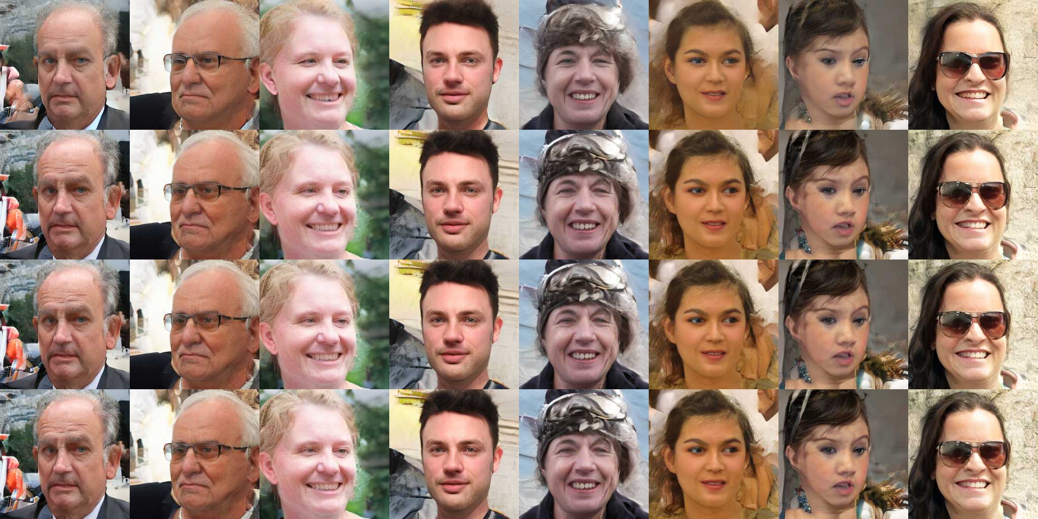
Figure 10: From top to bottom: 1, 2, 4 and 8 midpoint steps of inference using LeDiFlow on FFHQ [17].

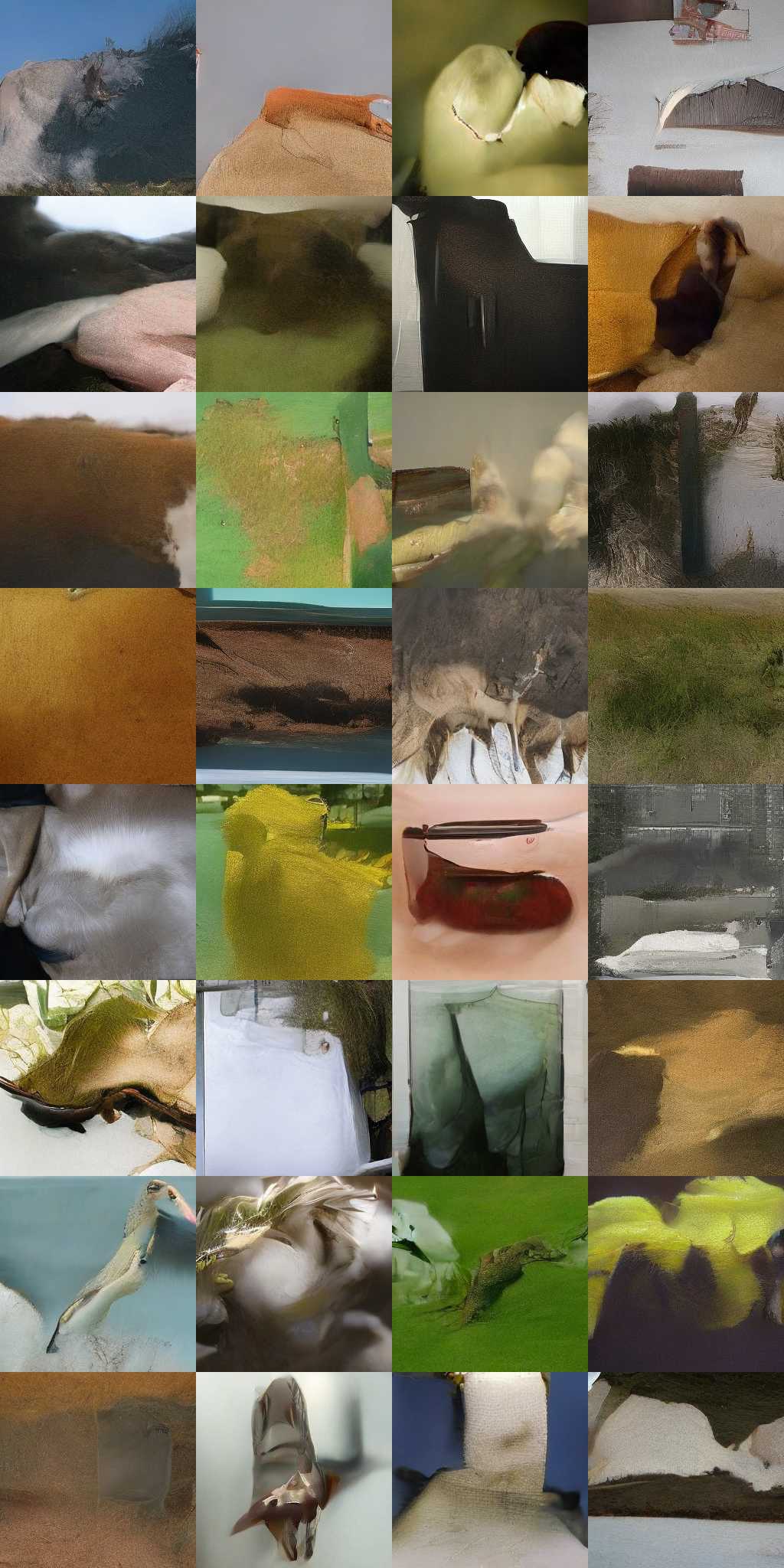
(a) LeDiFlow

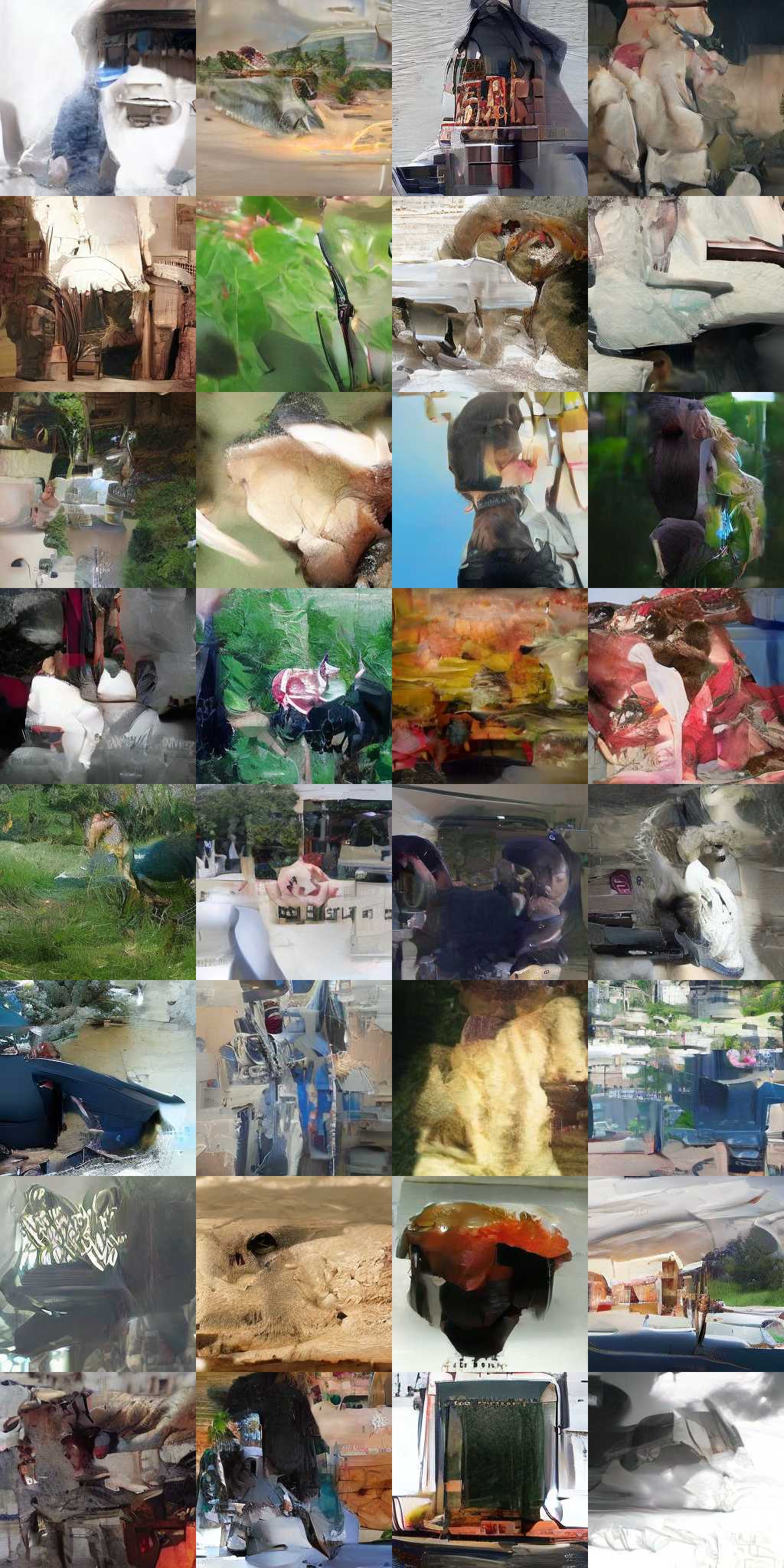
(b) FM

Figure 11: ImageNet [6] results using LeDiFlow and FM.

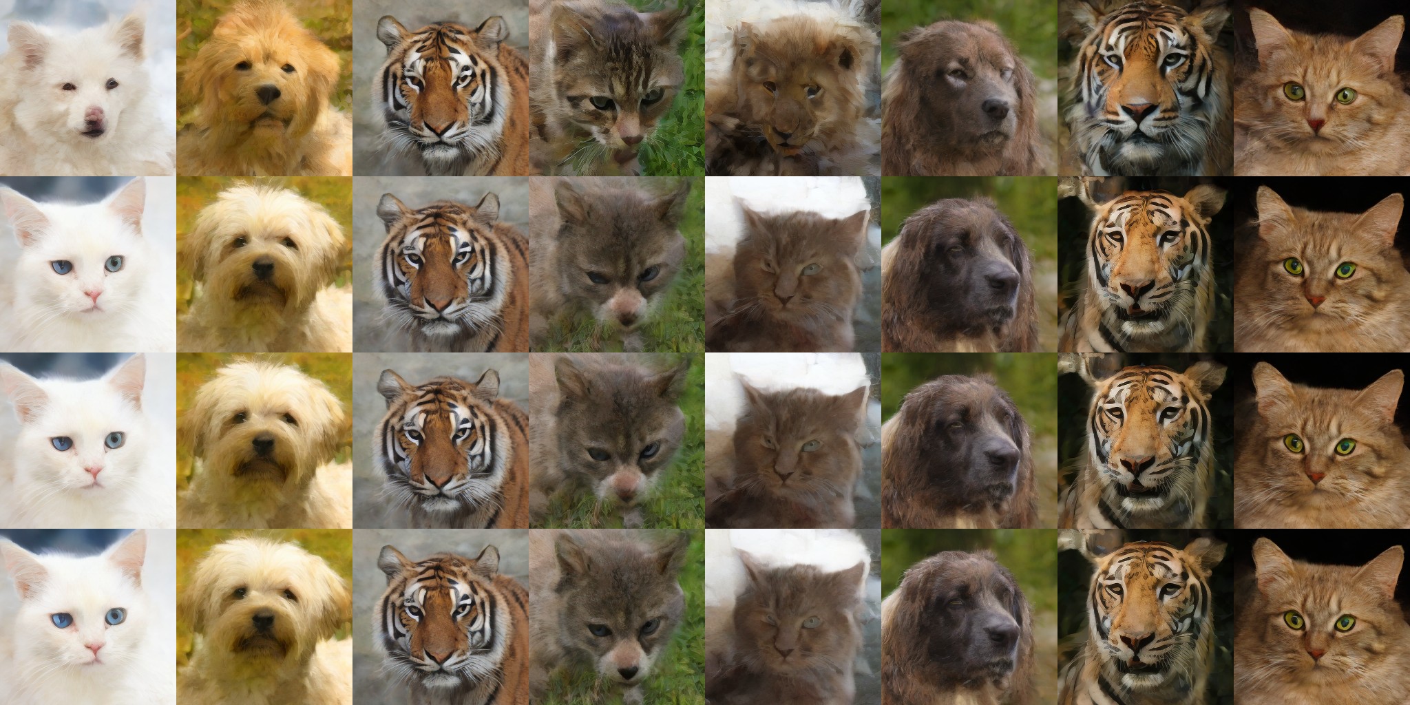
(a) AFHQ

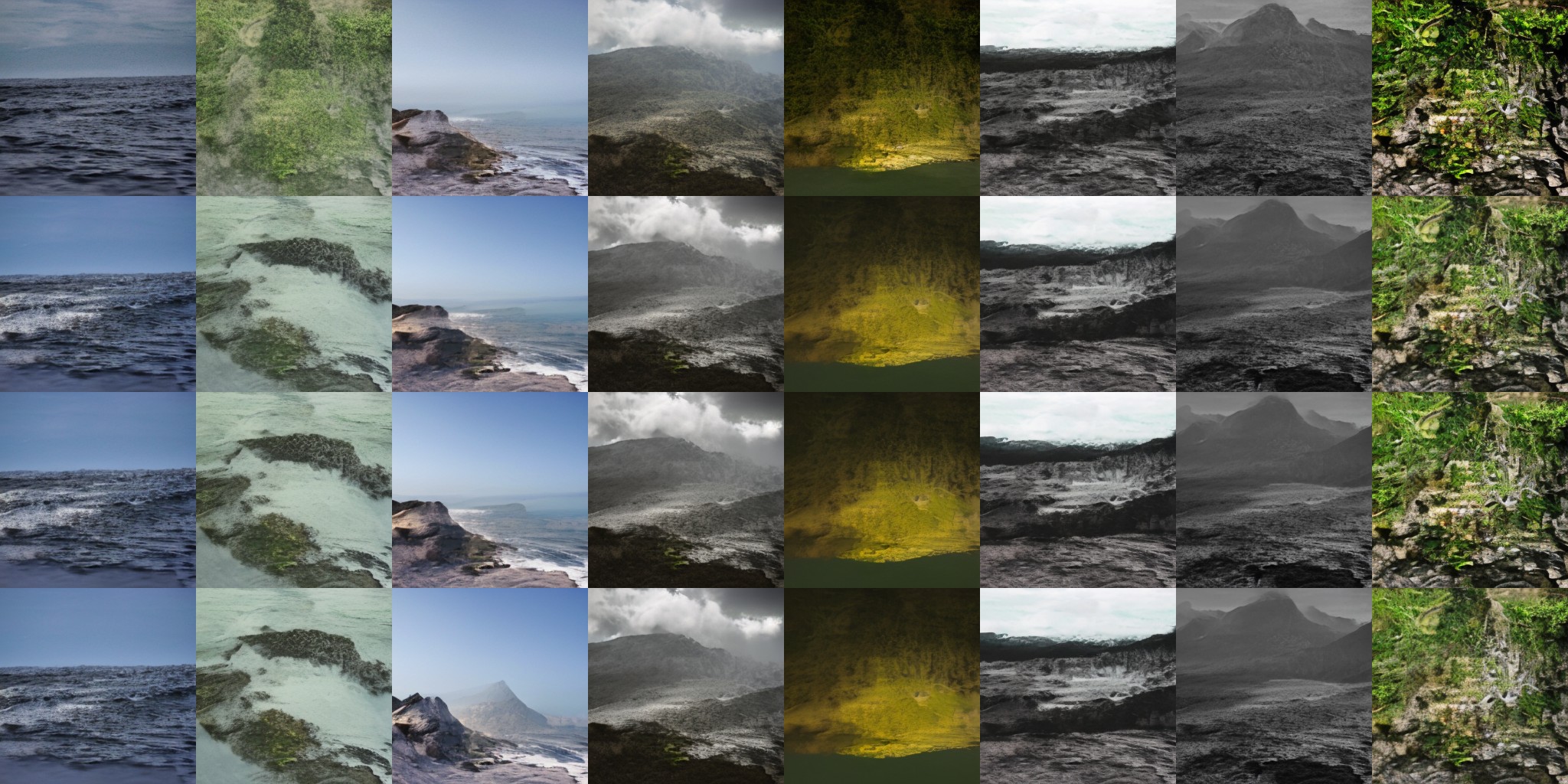
(b) LHQ

Figure 12: Images generated with varying number of steps of the latent sampler. From top to bottom: 1, 2, 4, and 8 steps.

Table 4: Licenses of Assets used in this work

Asset	License
FFHQ [17]	CC-BY-NC-SA 4.0
AFHQ [32]	CC-BY-NC 4.0
LHQ [3]	CC BY 2.0
ImageNet [6]	Custom Non Commercial
SDV [9]	CreativeML Open RAIL++-M License

References

- Butcher [1967] J. C. Butcher. Coefficients and error bounds for Runge-Kutta methods. Mathematics of Computation, 21(100):637–644, 1967. doi: 10.2307/2004864. URL https://doi.org/10.2307/2004864.
- Chen et al. [2018] T. Q. Chen, Y. Rubanova, J. Bettencourt, and D. Duvenaud. Neural ordinary differential equations. In Advances in Neural Information Processing Systems (NeurIPS), pages 6571–6583, 2018.
- Choi et al. [2020] Y. Choi, Y. Uh, J. Yoo, and J.-W. Ha. StarGAN v2: Diverse Image Synthesis for Multiple Domains. In Proceedings of the IEEE/CVF Conference on Computer Vision and Pattern Recognition (CVPR), pages 8188–8197, 2020.
- Conniffe [1987] D. Conniffe. Expected maximum log likelihood estimation. The Statistician, 36:317–329, 1987.
- Crowson et al. [2024] K. Crowson, S. A. Baumann, A. Birch, T. M. Abraham, D. Z. Kaplan, and E. Shippole. Scalable high-resolution pixel-space image synthesis with hourglass diffusion transformers. In Proceedings of the IEEE/CVF Conference on Computer Vision and Pattern Recognition (CVPR), pages 567–576, 2024. doi: 10.48550/arXiv.2401.11605.
- Deng et al. [2009] J. Deng, W. Dong, R. Socher, L.-J. Li, K. Li, and L. Fei-Fei. ImageNet: A large-scale hierarchical image database. In Proceedings of the IEEE/CVF Conference on Computer Vision and Pattern Recognition (CVPR), pages 248–255. IEEE, 2009.
- Dosovitskiy et al. [2021] A. Dosovitskiy, L. Beyer, A. Kolesnikov, D. Weissenborn, X. Zhai, T. Unterthiner, M. Dehghani, M. Minderer, G. Heigold, S. Gelly, J. Uszkoreit, and N. Houlsby. An image is worth 16x16 words: Transformers for image recognition at scale. In International Conference on Learning Representations, 2021. URL https://arxiv.org/abs/2010.11929.
- Esser et al. [2021] P. Esser, R. Rombach, and B. Ommer. Taming transformers for high-resolution image synthesis. In Proceedings of the IEEE/CVF Conference on Computer Vision and Pattern Recognition (CVPR), pages 12873–12883, 2021. doi: 10.48550/arXiv.2012.09841.
- Esser et al. [2024] P. Esser, S. Kulal, A. Blattmann, R. Entezari, J. Müller, H. Saini, Y. Levi, D. Lorenz, A. Sauer, F. Boesel, et al. Scaling rectified flow transformers for high-resolution image synthesis. In Forty-First International Conference on Machine Learning, 2024.
- Goodfellow et al. [2014] I. Goodfellow, J. Pouget-Abadie, M. Mirza, B. Xu, D. Warde-Farley, S. Ozair, A. Courville, and Y. Bengio. Generative adversarial networks. In Advances in Neural Information Processing Systems (NeurIPS), pages 2672–2680, 2014.
- Heusel et al. [2017] M. Heusel, H. Ramsauer, T. Unterthiner, B. Nessler, and S. Hochreiter. GANs Trained by a Two Time-Scale Update Rule Converge to a Local Nash Equilibrium. In Advances in Neural Information Processing Systems (NeurIPS), pages 6626–6637, 2017.
- Higgins et al. [2017] I. Higgins, L. Matthey, A. Pal, C. Burgess, X. Glorot, M. Botvinick, S. Mohamed, and A. Lerchner. Beta-VAE: Learning Basic Visual Concepts with a Constrained Variational Framework. In Proceedings of the 5th International Conference on Learning Representations (ICLR), 2017.
- Hinton and Salakhutdinov [2006] G. E. Hinton and R. R. Salakhutdinov. Reducing the dimensionality of data with neural networks. Science, 313(5786):504–507, 2006.
- Ho et al. [2020] J. Ho, A. Jain, and P. Abbeel. Denoising diffusion probabilistic models. Advances in Neural Information Processing Systems (NeurIPS), 33:6840–6851, 2020.
- Hukkelås and Lindseth [2023] H. Hukkelås and F. Lindseth. DeepPrivacy2: Towards Realistic Full-Body Anonymization. In Proceedings of the IEEE/CVF Winter Conference on Applications of Computer Vision (WACV), 2023.
- Jayasumana et al. [2023] S. Jayasumana, S. Ramalingam, A. Veit, D. Glasner, A. Chakrabarti, and S. Kumar. Rethinking FID: Towards a Better Evaluation Metric for Image Generation. In Proceedings of the IEEE/CVF Conference on Computer Vision and Pattern Recognition (CVPR), pages 1–12, 2023. URL https://arxiv.org/abs/2401.09603.
- Karras et al. [2019] T. Karras, S. Laine, and T. Aila. Flickr-Faces-HQ Dataset (FFHQ), 2019. URL https://github.com/NVlabs/ffhq-dataset.
- Karras et al. [2022] T. Karras, M. Aittala, T. Aila, and S. Laine. Elucidating the design space of diffusion-based generative models. In Proceedings of the Conference on Neural Information Processing Systems (NeurIPS), 2022. URL https://papers.nips.cc/paper/2022/hash/edm.pdf.
- Kingma and Welling [2014] D. P. Kingma and M. Welling. Auto-Encoding Variational Bayes. In Proceedings of the 2nd International Conference on Learning Representations (ICLR), 2014.
- Labs [2023] B. F. Labs. Flux.1: A rectified flow transformer for text-to-image generation. https://huggingface.co/black-forest-labs/FLUX.1-dev, 2023.
- Lee et al. [2023] S. Lee, B. Kim, and J. C. Ye. Minimizing trajectory curvature of ode-based generative models. In International Conference on Machine Learning, pages 18957–18973. PMLR, 2023.
- Li et al. [2022] J. Li, Y. Xu, T. Lv, L. Cui, C. Zhang, and F. Wei. DiT: Self-supervised Pre-training for Document Image Transformer. In Proceedings of the 30th ACM International Conference on Multimedia, pages 2975–2983. ACM, 2022. doi: 10.1145/3503161.3547999.
- Lipman et al. [2022] Y. Lipman, R. T. Chen, H. Ben-Hamu, M. Nickel, and M. Le. Flow matching for generative modeling. arXiv preprint arXiv:2210.02747, 2022.
- Liu et al. [2019] K. Liu, W. Tang, F. Zhou, and G. Qiu. Spectral Regularization for Combating Mode Collapse in GANs. In Proceedings of the IEEE/CVF International Conference on Computer Vision (ICCV), pages 6382–6390, 2019.
- Liu et al. [2022] X. Liu, C. Gong, and Q. Liu. Flow straight and fast: Learning to generate and transfer data with rectified flow. arXiv preprint arXiv:2209.03003, 2022.
- Nie and Patel [2019] W. Nie and A. B. Patel. Towards a Better Understanding and Regularization of GAN Training Dynamics. In Proceedings of the Conference on Uncertainty in Artificial Intelligence (UAI), pages 91–101, 2019. URL http://auai.org/uai2019/proceedings/papers/91.pdf.
- Pearson [1901] K. Pearson. On lines and planes of closest fit to systems of points in space. The London, Edinburgh, and Dublin Philosophical Magazine and Journal of Science, 2(11):559–572, 1901. doi: 10.1080/14786440109462720.
- Preechakul et al. [2022] K. Preechakul, N. Chatthee, S. Wizadwongsa, and S. Suwajanakorn. Diffusion autoencoders: Toward a meaningful and decodable representation. In Proceedings of the IEEE/CVF Conference on Computer Vision and Pattern Recognition (CVPR), pages 10619–10628, 2022.
- Rombach et al. [2022] R. Rombach, A. Blattmann, D. Lorenz, P. Esser, and B. Ommer. High-Resolution Image Synthesis with Latent Diffusion Models. In Proceedings of the IEEE/CVF Conference on Computer Vision and Pattern Recognition (CVPR), pages 10684–10695, 2022.
- Ronneberger et al. [2015] O. Ronneberger, P. Fischer, and T. Brox. U-Net: Convolutional Networks for Biomedical Image Segmentation. In Medical Image Computing and Computer-Assisted Intervention – MICCAI 2015, pages 234–241. Springer, Cham, 2015. doi: 10.1007/978-3-319-24574-4_28.
- Sauer et al. [2024] A. Sauer, D. Lorenz, A. Blattmann, and R. Rombach. Adversarial diffusion distillation. In Proceedings of the IEEE/CVF Conference on Computer Vision and Pattern Recognition (CVPR), 2024. URL https://arxiv.org/abs/2311.17042.
- Skorokhodov et al. [2021] I. Skorokhodov, G. Sotnikov, and M. Elhoseiny. Aligning latent and image spaces to connect the unconnectable. arXiv preprint arXiv:2104.06954, 2021.
- van den Oord et al. [2017] A. van den Oord, O. Vinyals, and K. Kavukcuoglu. Neural Discrete Representation Learning. In Proceedings of the Conference on Neural Information Processing Systems (NeurIPS), pages 6306–6315, 2017. URL https://arxiv.org/abs/1711.00937.
- Vaswani et al. [2017] A. Vaswani, N. Shazeer, N. Parmar, J. Uszkoreit, L. Jones, A. N. Gomez, L. Kaiser, and I. Polosukhin. Attention is all you need. In Advances in Neural Information Processing Systems (NeurIPS), pages 5998–6008, 2017.
- Zhang et al. [2023] L. Zhang, A. Rao, and M. Agrawala. Adding conditional control to text-to-image diffusion models. In Proceedings of the IEEE/CVF International Conference on Computer Vision (ICCV), 2023.
- Zwick et al. [2024] P. Zwick, K. Roesch, M. Klemp, and O. Bringmann. Context-aware full body anonymization using text-to-image diffusion models. In Proceedings of the 12th International Workshop on Assistive Computer Vision and Robotics (ACVR) in conjunction with ECCV, 2024.
Glossary
- AE
- Autoencoder
- AFHQ
- Animal Faces-HQ
- CMMD
- CLIP Maximum Mean Discrepancy
- DiT
- Diffusion Transformer
- DM
- Diffusion Model
- FFHQ
- Flickr-Faces-HQ
- FID
- Frechet Inception Distance
- FM