Probabilistic Kernel Function for Fast Angle Testing

Abstract

In this paper, we study the angle testing problem in high-dimensional Euclidean spaces and propose two projection-based probabilistic kernel functions, one designed for angle comparison and the other for angle thresholding. Unlike existing approaches that rely on random projection vectors drawn from Gaussian distributions, our approach leverages reference angles and employs a deterministic structure for the projection vectors. Notably, our kernel functions do not require asymptotic assumptions, such as the number of projection vectors tending to infinity, and can be both theoretically and experimentally shown to outperform Gaussian-distribution-based kernel functions. We further apply the proposed kernel function to Approximate Nearest Neighbor Search (ANNS) and demonstrate that our approach achieves a 2.5X $\sim$ 3X higher query-per-second (QPS) throughput compared to the state-of-the-art graph-based search algorithm HNSW.

1 Introduction

Vector-based similarity search is a core problem with broad applications in machine learning, data mining, and information retrieval. It involves retrieving data points in high-dimensional space that are most similar to a given query vector based on a specific similarity measure. This task is central to many downstream applications, including nearest neighbor classification, recommendation systems, clustering, anomaly detection, and large-scale information retrieval. However, the high dimensionality of modern datasets makes efficient similarity search particularly challenging, highlighting the need for fast and scalable vector computation techniques.

Among the various similarity measures for high-dimensional vectors, the $\ell_{2}$ norm, cosine distance, and inner product are the most commonly used in practice. As discussed in Norm_range_LSH ; norm-explicit-quantization ; peos , it is often possible to pre-compute and store the norms of vectors in advance, allowing these measures to be reduced to the computation of the angle (inner product) between two normalized vectors, thereby highlighting the central role of angle computation. On the other hand, in many real-world scenarios, we are not concerned with the exact value of the angle itself but rather with the outcome of an angle-based comparison, which is referred to as the angle testing. Specifically, given a query vector $\bm{q}$ and data vectors $\bm{v_{1}}$, $\bm{v_{2}}$, $\bm{v}$ on sphere $\mathbb{S}^{d-1}$, typical operations include comparing $\left\langle\bm{q},\bm{v_{1}}\right\rangle$ and $\left\langle\bm{q},\bm{v_{2}}\right\rangle$, or determining whether $\left\langle\bm{q},\bm{v}\right\rangle$ exceeds a certain threshold. These operations, however, require computing exact inner products, which have a cost of $O(d)$ per comparison and become expensive in high dimensions. To address this, we aim to design a computation-efficient probabilistic kernel function $K$ that can approximate these comparisons with reduced cost and high success probability. In particular, we focus on the following two problems:

Problem 1.1

(Probabilistic kernel function for comparison) Given $\bm{q}$, $\bm{v_{1}}$ and $\bm{v_{2}}$ on $\mathbb{S}^{d-1}$, where $\left\langle\bm{q},\bm{v_{1}}\right\rangle>\left\langle\bm{q},\bm{v_{2}}\right\rangle$, how can we design a probabilistic kernel function $K(\cdot,\cdot):\mathbb{S}^{d-1}\times\mathbb{S}^{d-1}\rightarrow\text{RV}$, where RV denotes the set of real-valued random variables, such that (1) the computation of $K(\bm{q},\bm{v})$ does not rely on the computation of $\left\langle\bm{q},\bm{v}\right\rangle$, and (2) $\mathbb{P}[K(\bm{q},\bm{v_{1}})>K(\bm{q},\bm{v_{2}})]$ is as high as possible?

Problem 1.2

(Probabilistic kernel function for thresholding) Given an arbitrary pair of normalized vectors $(\bm{q},\bm{v})$ with an angle $\phi$, and an angle threshold $\theta$, how can we design a probabilistic kernel function $K(\cdot,\cdot):\mathbb{S}^{d-1}\times\mathbb{S}^{d-1}\rightarrow\text{RV}$ such that (1) the computational complexity of $K(\bm{q},\bm{v})$ is significantly lower than that of computing the exact inner product $\left\langle\bm{q},\bm{v}\right\rangle$, and (2) $K(\bm{q},\bm{v})$ can reliably determine whether $\phi$ is smaller than $\theta$ with a high success probability?

Both problems have various applications. The goal of Problem 1.1 aligns with that of CEOs ceos under cosine distance (we will postpone the general case of inner product to Sec. 4), allowing the designed kernel function to be applied to tasks where CEOs is effective, such as Maximum Inner Product Search (MIPS) ceos , filtering of NN candidates Falconn++ , DBSCAN sDBSCAN , and more. On the other hand, the goal of Problem 1.2 is similar to that of PEOs peos , making the corresponding kernel function well-suited for probabilistic routing tests in similarity graphs, which have demonstrated significant performance improvements over original graphs, such as HNSW hnsw . In Sec. 4, we will further elaborate on the applications of these two probabilistic kernel functions.

Despite addressing different tasks, all the techniques ceos ; Falconn++ ; sDBSCAN ; peos mentioned above use Gaussian distribution to generate projection vectors and are built upon a common statistical result, as follows.

Lemma 1.3

(Theorem 1 in ceos ) Given two vectors $\bm{v}$, $\bm{q}$ on $\mathbb{S}^{d-1}$, and $m$ random vectors $\{\bm{u}_{i}\}^{m}_{i=1}\sim\mathcal{N}(0,I^{d})$, and $m$ is sufficiently large, assuming that $\bm{u}_{\mathrm{max}}={\mathop{\rm argmax}_{\bm{u_{i}}}}|\bm{q}^{\top}\bm{u_{i}}|$, we have:

$$\bm{v}^{\top}\bm{u}_{\mathrm{max}}\sim\mathcal{N}({\mathop{\rm sgn}}(\bm{q}^{\top}\bm{u}_{\mathrm{max}})\cdot\bm{q}^{\top}\bm{v}\sqrt{2\ln m},1-(\bm{q}^{\top}\bm{v})^{2}).$$ (1)

Lemma 1.3 builds the relationship between angles and corresponding projection vectors. Actually, $\bm{v}^{\top}\bm{u_{\text{max}}}$ can be viewed as an indicator of the cosine angle $\bm{q}^{\top}\bm{v}$. More specifically, the larger $\bm{v}^{\top}\bm{u_{\text{max}}}$ is, the more likely it is that $\bm{q}^{\top}\bm{v}$ is large. On the other hand, $\bm{v}^{\top}\bm{u_{\text{max}}}$ can be computed beforehand during the indexing phase and can be easily accessed during the query phase, making $K(\bm{q},\bm{v})=\bm{v}^{\top}\bm{u_{\text{max}}}$ a suitable kernel function for various angle testing problems, e.g., Problem 1.1.

However, Lemma 1.3 has a significant theoretical limitation: the relationship (1) relies on the assumption that the number of projection vectors $m$ tends to infinity. Since the evaluation time of projection vectors depends on $m$, $m$ cannot be very large in practice. Moreover, since Falconn++ ; sDBSCAN ; peos all used Lemma 1.3 to derive their respective theoretical results, these results are also affected by this limitation, and the impact of $m$ becomes even harder to predict in these applications.

The starting point of our research is to overcome this limitation, and we make the following two key observations. (1) The Gaussian distribution used in Lemma 1.3 is not essential. In fact, the only factor determining the estimation accuracy of $\bm{q}^{\top}\bm{v}$ is the reference angle, that is, the angle between $\bm{q}$ and $\bm{u_{\text{max}}}$. (2) By introducing a random rotation matrix, the reference angle becomes dependent on the structure of the projection vectors and is predictable.

Based on these two observations, we design new probabilistic kernel functions to solve problems 1.1 and 1.2. Specifically, the contributions of this paper are summarized as follows.

(1) The proposed kernel functions $K^{1}_{S}$ and $K^{2}_{S}$ (see eq. (2) and eq. (3)) rely on a reference-angle-based probabilistic relationship between angles in high-dimensional spaces and projected values. Compared with eq. (1), the new relationship (see relationship (4)) is deterministic without dependence on asymptotic condition. By theoretical analysis, we show that, the proposed kernel functions are effective for the Problems 1.1 and 1.2, and the smaller the reference angle is, the more accurate the kernel functions are (see Lemmas 3.2 and 3.3 ).

(2) To minimize the reference angle, we study the structure of the configuration of projection vectors (see Sec. 3.2). We propose two structures (see Alg. 1 and Alg. 2) that perform better than purely random projection (see Alg. 3), and we establish the relationship between the reference angle and the proposed structures (see Lemma 3.5 and Fig. 4).

(3) Based on $K^{1}_{S}$, we propose a random-projection technique KS1 which can be used for CEOs-based tasks ceos ; Falconn++ ; sDBSCAN . Based on $K^{2}_{S}$, we introduce a new routing test called the KS2 test which can be used to accelerate the graph-based Approximate Nearest Neighbor Search (ANNS) peos (see Sec. 4).

(4) We experimentally show that KS1 provides a slight accuracy improvement (up to 0.8%) over CEOs. In the ANNS task, we demonstrate that HNSW+KS2 improves the query-per-second (QPS) of the state-of-the-art approach HNSW+PEOs peos by 10% – 30%, along with a 5% reduction in index size.

2 Related Work

Due to space limitations, we focus on random projection techniques that are closely related to this work. An illustration comparing the proposed random projection technique with others can be found in Sec. B.1 and Fig. 3 in Appendix. Since the proposed kernel function is also used in similarity graphs for ANNS, a comprehensive discussion of ANNS solutions is provided in Appendix B.2.

In high-dimensional Euclidean spaces, the estimation of angles via random-projection techniques, especially Locality Sensitive Hashing (LSH) IndykM98:approximate-nearest-neighbor ; Andoni2004:e2lsh ; AndoniI08:near-optimal-hashing , has a relatively long history. One classical LSH-based technique is SimHash simhash , whose basic idea is to generate multiple hyperplanes and partition the original space into many cells such that two vectors falling into the same cell are likely to have a small angle between them. In falconn , the authors proposed a different LSH-based technique called Falconn for angular distance, whose basic idea is to find the closest or furthest projection vector to the data vector and record this projection vector as a hash value, leading to better search performance than SimHash. Later, the authors in ceos employed Concomitants of Extreme Order Statistics (CEOs) to identify the projection with the largest or smallest inner product with the data vector, as shown in Lemma 1.3, and recorded the corresponding maximum or minimum projected value to obtain a more accurate estimation than using a hash value alone Falconn++ . Notably, CEOs can be used not only for angular distance but also for inner product estimation.

Due to its ease of implementation, CEOs has been employed in several similarity search tasks ceos ; falconn ; sDBSCAN , as mentioned in Sec. 1. Additionally, CEOs has been used to accelerate similarity graphs, which are among the leading structures for Approximate Nearest Neighbor Search (ANNS). In peos , by swapping the roles of query and data vectors in CEOs, the authors introduced a space-partitioning technique and proposed the PEOs test, which can be used to compare the objective angle with a fixed threshold under probabilistic guarantees. This test was incorporated into the routing mechanisms of similarity graphs and achieved significant search performance improvements over original graph structures like HNSW hnsw and NSSG nssg .

3 Two Probabilistic Kernel Functions

3.1 Reference-Angle-Based Design

In Sec. 3.1, we aim to propose probabilistic kernel functions for Problems 1.1 and 1.2. First, we introduce some notation. Let $\mathbb{R}^{d}$ be the ambient vector space. Define $H\in SO(d)\in\mathbb{R}^{d\times d}$ as a random rotation matrix (Note that the definition here differs from that in falconn , where the so-called random rotation matrix is actually a matrix with i.i.d. Gaussian entries), and let $S=[\bm{u_{1}},\bm{u_{2}},\ldots,\bm{u_{m}}]\in\mathbb{R}^{d\times m}$ be an arbitrary fixed set of $m$ points on the unit sphere $\mathbb{S}^{d-1}$. For any vector $\bm{v}\in\mathbb{S}^{d-1}$, define the reference vector of $\bm{v}$ with respect to $S$ as $Z_{S}(\bm{v})=\mathop{\rm argmax}_{\bm{u}\in S}\left\langle\bm{u},\bm{v}\right\rangle$. Let $A_{S}(\bm{v})$ denote the cosine of the reference angle with respect to $Z_{S}(\bm{v})$, that is, $A_{S}(\bm{v})=\left\langle\bm{v},Z_{S}(\bm{v})\right\rangle$ . Next, we introduce two probabilistic kernel functions $K^{1}_{S}(\cdot,\cdot)$ and $K^{2}_{S}(\cdot,\cdot)$ as follows, where $K^{1}_{S}(\cdot,\cdot)$ corresponds to Problem 1.1 and $K^{2}_{S}(\cdot,\cdot)$ corresponds to Problem 1.2.

$$K^{1}_{S}(\bm{q},\bm{v})=\left\langle\bm{v},Z_{HS}(\bm{q})\right\rangle\qquad\bm{v},\bm{q}\in\mathbb{S}^{d-1}.$$ (2)

$$K^{2}_{S}(\bm{q},\bm{v})=\left\langle H\bm{q},Z_{S}(H\bm{v})\right\rangle/A_{S}(H\bm{v})\qquad\bm{v},\bm{q}\in\mathbb{S}^{d-1}.$$ (3)

Remarks. (1) (Computational efficiency) Both functions are computationally efficient. For $K^{1}_{S}(\bm{q},\bm{v})$, $HS$ and $\left\langle\bm{v},H\bm{u_{i}}\right\rangle$ ($1\leq i\leq m$) can be pre-computed. Hence, for all $\bm{v}$’s, we only need to determine $Z_{HS}(\bm{q})$ online, which requires cost $O(dm)$ (This cost can be further reduced by a reasonable choice of $S$. See Sec. 3.2). For $K^{2}_{S}(\bm{q},\bm{v})$, $A_{S}(H\bm{v})$ and $Z_{S}(H\bm{v})$ can be pre-computed. $H\bm{q}$ only needs to be computed online via Fast Johnson–Lindenstrauss Transform ACHash ; falconn once, with cost $O(d\log d)$, and $\left\langle H\bm{q},Z_{S}(H\bm{v})\right\rangle$ can be computed online with cost $O(L)$ for every $\bm{v}$, where $L\ll d$ denotes the number of partitioned subspaces and will be explained in Sec. 3.2.

(2) (Exploitation of reference angle) In the design of existing projection techniques such as CEOs ceos , Falconn falconn , Falconn++ Falconn++ , etc., only the reference vector $Z_{S}{(\cdot))}$ is utilized. In contrast, our kernel functions defined in eq. (2) and eq. (3) incorporate not only the reference vector $Z_{S}{(\cdot))}$ but also the reference angle information $A_{S}(\cdot)$ (although the reference angle is not explicitly shown in eq. (2), its influence will become clear in Lemma 3.2). In fact, the reference angle plays a central role, as it is the key factor controlling the precision of angle estimation (see Lemma 3.2).

(3) (Generalizations of CEOs and PEOs) Beyond incorporating the reference angle, these two kernel functions can also be regarded as generalizations of CEOs and PEOs respectively in a certain sense. Specifically, if $S$ is taken as a point set generated via a Gaussian distribution and $Z_{S}(\bm{v})$ is replaced by the reference vector having the maximum inner product with the query, then $K^{1}_{S}(\bm{q},\bm{v})$ equals the indicator $\bm{v}^{\top}\bm{u_{\text{max}}}$ used in CEOs. Similarly, if we remove the term $A_{S}(H\bm{v})$ and take $S$ to be the same space-partitioned structure as that of PEOs, $K^{2}_{S}(\bm{q},\bm{v})$ is similar to the indicator of PEOs.

(4) (Configuration of projection vectors) Although we do not currently require any specific properties of the configuration of $S$, it is clear that the shape of $S$ impacts both $K^{1}_{S}(\bm{q},\bm{v})$ and $K^{2}_{S}(\bm{q},\bm{v})$. We will discuss the structure of $S$ in detail in Sec. 3.2.

Next, we provide a definition that will be used to establish the property of $K^{2}_{S}$.

Definition 3.1

Let $\phi_{1},\phi_{2}\in(0,\pi)$ and let $\theta\in(0,\pi)$ be an arbitrary angle threshold. A probabilistic kernel function $K(\bm{q},\bm{v})$ is called angle-sensitive when it satisfies the following two conditions:

(1)If $\cos\theta\leq\cos\phi_{1}=\left\langle\bm{q},\bm{v}\right\rangle$, then $\mathbb{P}[K(\bm{q},\bm{v})\geq\cos\theta]\geq p_{1}(\phi_{1})$

(2)If $\left\langle\bm{q},\bm{v}\right\rangle=\cos\phi_{2}<\cos\theta$, then $\mathbb{P}[K(\bm{q},\bm{v})\geq\cos\theta]<p_{2}(\phi_{2})$

, where $p_{2}(\phi_{2})$ is a strictly decreasing function in $\phi_{2}$ and $p_{1}(\phi_{1})>p_{2}(\phi_{2})$ when $\phi_{1}<\phi_{2}$.

The definition of the angle-sensitive property is analogous to that of the locality-sensitive hashing property. The key difference is that the approximation ratio $c$ used in LSH is not introduced here, as the angle threshold $\theta$ is explicitly defined, and only angles smaller than $\theta$ are considered valid.

We are now ready to present the following two lemmas for $K^{1}_{S}$ and $K^{2}_{S}$, which demonstrate that they serve as effective solutions to Problems 1.1 and 1.2, respectively.

Lemma 3.2

(1) Let $d\geq 3$ and $(\bm{q},\bm{v})$ be an arbitrary pair of normalized vectors with angle $\phi\in(0,\pi)$. The conditional CDF of $K^{1}_{S}(\bm{q},\bm{v})$ can be expressed as follows:

$$F_{K^{1}_{S}(\bm{q},\bm{v})\mid A_{S}(\bm{q})}(x\mid\cos\psi)=I_{t}(\frac{d-2}{2},\frac{d-2}{2})$$ (4)

where $\psi\in(0,\pi)$, $t=\frac{1}{2}+\frac{x-\cos\phi\cos\psi}{2\sin\phi\sin\psi}$, $I_{t}$ denotes the regularized incomplete Beta function and $x\in[\cos(\phi+\psi),\cos(\phi-\psi)]$.

(2)Let $\bm{q}$, $\bm{v_{1}}$ and $\bm{v_{2}}$ be three normalized vectors on $\mathbb{S}^{d-1}$ such that $\left\langle\bm{q},\bm{v_{1}}\right\rangle>\left\langle\bm{q},\bm{v_{2}}\right\rangle$. The probability $\mathbb{P}[K^{1}_{S}(\bm{q},\bm{v_{1}})>K^{1}_{S}(\bm{q},\bm{v_{2}})|A_{S}(\bm{q})=\cos\psi]$ increases as $\psi$ decreases in $(0,\pi)$. In particular, when $\psi\in(0,\pi/2)$, $P[K^{1}_{S}(\bm{q},\bm{v_{1}})>K^{1}_{S}(\bm{q},\bm{v_{2}})|A_{S}(\bm{q})=\cos\psi]>0.5$.

Lemma 3.3

Let $\psi\in(0,\pi/2)$, that is, $A_{S}(\bm{v})=\cos\psi\in(0,1)$, and $d\geq 3$. Then $K^{2}_{S}$ is an angle-sensitive function, where $p_{1}(\phi)=0.5$ and $p_{2}(\phi)=I_{t^{\prime}}(\frac{d-2}{2},\frac{d-2}{2})$, where $t^{\prime}=\frac{1}{2}-\frac{\cos\theta-\cos\phi}{2\sin\phi\tan\psi}$.

Remarks. (1) (Discussion on boundary values) When $\phi=0$ or $\phi=\pi$, $K^{1}_{S}$ and $K^{2}_{S}$ take fixed values rather than being random variables, and when $\psi=0$ or $\psi=\pi$, the exact value of $\left\langle\bm{q},\bm{v}\right\rangle$ can be directly obtained. Therefore, probability analysis in these cases is meaningless. Additionally, in Lemma 3.3, we adopt the following convention: $p_{2}(\phi)=0$ if $t^{\prime}<0$.

(2) (Deterministic relationship for angle testing) Lemma 3.2 establishes a relationship between the objective angle $\phi$ and the value of the function $K^{1}_{S}$. Notably, after computing $Z_{S}(\cdot)$, the value of reference angle $A_{S}(\cdot)$ can be obtained automatically. Besides, as will be shown in Sec. 3.2, with a reasonable choice of $S$, the assumption $A_{S}(\cdot)>0$ can always be ensured. Hence, eq. (4) essentially describes a deterministic relationship. In contrast to the asymptotic relationship of CEOs, eq. (4) provides an exact relationship without additional assumptions.

(3) (Effectiveness of kernel functions) The above two lemmas show that, with a reasonable construction of $S$ such that the reference angle is small with high probability, $K^{1}_{S}$ and $K^{2}_{S}$ can effectively address the corresponding angle testing problems. Specifically, the smaller the reference angle is, the more effective $K^{1}_{S}$ and $K^{2}_{S}$ become (By $p_{2}(\phi)$, a smaller $\psi$ leads to a smaller $p_{2}(\phi)$).

(4) (Gaussian distribution is suboptimal) The fact that a smaller reference angle is favorable justifies the utilization of $Z_{S}(\cdot)$ and also implies that the Gaussian distribution is not an optimal choice for configuring $S$, since in this case, the selected reference vector with the largest inner product with the query or data vector is not guaranteed to have the smallest reference angle.

3.2 Configuration of Points Set on Hypersphere

The remaining task is to configure the set $S$. Given $m$, our goal is to construct a set $S$ of $m$ points on $\mathbb{S}^{d-1}$, denoted by $S_{m}$, such that the reference angle $A_{S_{m}}(\cdot)$ is minimized. Due to the effect of the random rotation matrix $H$, the optimal configurations denoted by $\bar{S}_{m}$ and ${S}_{m}^{*}$, can be obtained either in the sense of expectation or in the sense of the worst case, respectively. That is,

$$\bar{S}_{m}=\mathop{\rm argmax}_{S=\{u_{1},\dots,u_{m}\}\subset\mathbb{S}^{d-1}}\{{\mathbb{E}_{v\in U(\mathbb{S}^{d})}[A_{S}(\bm{v})]}\}.$$ (5)

$${S}_{m}^{*}=\underset{S=\begin{subarray}{c}\{u_{1},\dots,u_{m}\}\subset\mathbb{S}^{d-1}\end{subarray}}{\arg\max}\;\min_{v\in\mathbb{S}^{d-1}}\max_{1\leq i\leq m}\langle\bm{u_{i}},\bm{v}\rangle.$$ (6)

By the definitions of $\bar{S}_{m}$ and ${S}_{m}^{\ast}$, they correspond to the configurations that achieve the smallest expected value and the smallest maximum value of $A_{S}(\bm{v})$, respectively. On the other hand, finding the exact solutions for $\bar{S}_{m}$ and ${S}_{m}^{\ast}$ is closely related to the best covering problem on the sphere, which is highly challenging and remains open in the general case. To the best of the authors’ knowledge, the optimal configuration ${S}_{m}^{\ast}$ is only known when $m\leq d+3$. In light of this, we provide two configurations of $S$: one relies on random antipodal projections (Alg. 1), and the other is built using multiple cross-polytopes (Alg. 2). Each has its own advantages. Specifically, Alg. 1 enables the estimation of reference angles, while Alg. 2 can empirically produce slightly smaller reference angles and is more efficient for projection computation.

Algorithm 1 Configuration of $S$ via antipodal projections

Input: $L$ is the level; $d=Ld^{\prime}$ is the data dimension; $m$ is the number of vectors in each level

Output: $S_{\text{sym}}(m,L)$, which is represented by $mL$ sub-vectors with dimension $d^{\prime}$.

for $l=1$ to $L$ do

2    Generate $m/2$ points along with their antipodal points i.i.d. on $S^{d^{\prime}-1}$  Scale the norm of all $m$ points in this iteration to $1/\sqrt{L}$, and collect the vectors after scaling 

Algorithm 2 Configuration of $S$ via multiple cross-polytopes

Input: $L$ is the level; $d=Ld^{\prime}$ is the data dimension; $m=2d^{\prime}a+b$; $R$ is the maximum number of iterations

Output: $S_{\text{pol}}(m,L)$, which is represented by $mL$ sub-vectors with dimension $d^{\prime}$

Generate $N$ points randomly and independently on $\mathbb{S}^{d-1}$, where $N$ is a sufficiently large number

for $r=1$ to $R$ do

4    for $t=1$ to $a$ do

5       Generate a random rotation matrix $H\in\mathbb{R}^{d^{\prime}\times d^{\prime}}$, and rotate $2d$ axes in $\mathbb{R}^{d^{\prime}}$ using $H$  Collect the $2d$ vectors of the cross-polytope after rotation 

6   if $b>0$ then

7       Repeat the above iteration and select $b/2$ antipodal pairs from the rotated cross-polytope 

8   For the generated $S\in\mathbb{S}^{d^{\prime}-1}$, compute $\tilde{J}(S,N)$ and maintain the largest $S$ denoted by $S_{\text{max}}$

9for $l=1$ to $L$ do

10    Generate a random rotation matrix $H\in\mathbb{R}^{d^{\prime}\times d^{\prime}}$ and rotate the configuration $S_{\text{max}}$ using $H$  Scale the norm of all $m$ points in this iteration to $1/\sqrt{L}$ and collect the vectors after scaling 

Before proceeding into the detail of algorithms, we introduce a quantity $J(S)$ as follows.

$$J(S)=\mathbb{E}_{v\in U(\mathbb{S}^{d})}[(A_{S}(\bm{v}))].$$ (7)

By definition, $J(S)$ denotes the expected value of the cosine of the reference angles w.r.t $S$. This quantity is consistent with our theory, as a random rotation is applied to $\bm{v}$ or $\bm{q}$ in eq. (2) and eq. (3). Based on the previous analysis, for a fixed $m$, $J(S)$ is minimized when $S=\bar{S}_{m}$, which is hard to compute. However, we have the following result to approximately evaluate $J(S)$.

Lemma 3.4

For every integer $N\geq 1$, let $v_{1,N},\ldots,v_{N,N}$ be the vectors randomly and independently drawn from $U(\mathbb{S}^{d})$. Let $\tilde{J}(S,N)=[\Sigma_{i=1}^{N}A_{S}(\bm{v_{i,N}})]/N$. $\tilde{J}(S,N)\xrightarrow{p}J(S)$ as $N$ goes infinity.

Lemma 3.4 shows that, when $N$ is sufficiently large, we can approximately evaluate the performance of different configurations $S$’s by comparing their $\tilde{J}(S,N)$’s.

Now, we are ready to explain Alg. 1 and Alg. 2 as follows.

(1) (Utilization of antipodal pairs and cross-polytopes) We use the antipodal pair or the cross-polytope as our building block for the following three reasons. (1) Since all the projection vectors are antipodal pairs, the evaluation time of projection vectors can be halved. (2) Both of two structures can ensure that the assumption $A_{S}(\bm{v})>0$ holds, such that the condition in Lemma 3.3 is always satisfied. (3) The result in antipodal-result shows that, for $m=2d$, under mild conditions, the $2d$ vertices of a cross-polytope can be proven to have the smallest covering radius, that is, the smallest reference angle in the worst case. Although the results in the case $m>2d$ are unknown, we can rotate the fixed cross-polytope in random directions to generate multiple cross-polytopes until we obtain $m$ vectors, which explains the steps from 6 to 10 in Alg. 2.

(2) (Selection from random configurations) We can generate such $m$ points in the above way many times, which forms multiple $S$’s. By Lemma 3.4, we can use $\tilde{J}(S,N)$ to approximately evaluate the performance of $J(S)$, and thus, among the generated $S$’s, we select the configuration $S_{\text{pol}}$ corresponding to the maximal $\tilde{J}(S,n)$. This explains steps 5 and 11 in Alg. 2.

(3) (Accuracy boosting via multiple levels) Clearly, increasing $m$ can lead to a smaller reference angle. The analysis in peos shows that, for certain angle-thresholding problems requiring high accuracy, an exponential increase in $m$, rather than a linear one, can be effective. Therefore, similar to peos , we use a product-quantization-like technique PQ to partition the original space into $L$ subspaces (levels), which is adopted in both algorithms. By concatenating equal-length sub-vectors from these $L$ subspaces, we can virtually generate $m^{L}$ normalized projected vectors. As will be shown in Lemma 3.5, the introduction of $L$ can significantly decrease the reference angle.

(4) (Fast projection computation via multi-cross-polytypes) In eq. (2) and eq. (3), we need to compute $H\bm{q}$, $H\bm{v}$, $HS\bm{q}$ and $HS\bm{v}$ in the indexing phase or in the query phase. If such projection time is a concern in practice, we can set $R$ and $L$ to 1 in Alg. 2 to accelerate the projection without the explicit computation of $S$. Specifically, if $m\geq 2d$, suppose that $m$ is divisible by $2d$ and $m=2ld$. $H^{\top}$ or $(HS)^{\top}$ can be approximated by $[S_{(1)},S_{(2)},S_{(l)}]^{\top}$, where $S_{(i)}$ here denotes the $i$-th structured random projection matrix. Then the projection time cost for $v$ or $q$ can be reduced from $O(md)$ to $O((m\log d)/2)$. If $2d>m$, the cost is $O(d\log d)$ by the projection matrix completion.

By Alg. 1 and Alg. 2, we obtain structures $S_{\text{sym}}(m,L)$ and $S_{\text{pol}}(m,L)$ virtually containing $m^{L}$ projection vectors. For $S_{\text{sym}}(m,L)$, we can establish a relationship between $J(S_{\text{sym}}(m,L))$ and $(m,L)$ as follows, which reveals the impact of the choice of $(m,L)$ on reference angle.

Lemma 3.5

Suppose that $d$ is divisible by $L$, and $d=Ld^{\prime}$, where $d^{\prime}\geq 3$. Let $c_{d^{\prime}}=\frac{\Gamma\left(\frac{d^{\prime}}{2}\right)}{\sqrt{\pi}\,\Gamma\left(\frac{d^{\prime}-1}{2}\right)}$, $f(y)=c_{d}^{\prime}(1-y^{2})^{\frac{d^{\prime}-3}{2}}$ and $F(y)=\int_{-1}^{y}f(t)\,dt$. We have

$$J(S_{\mathrm{sym}}(m,L))>m\sqrt{L}\frac{\Gamma(\frac{d+L}{2L})\Gamma(\frac{d}{2})}{\Gamma(\frac{d}{2L})\Gamma(\frac{d+1}{2})}\int_{-1}^{1}yF(y)^{m-1}f(y)\,\mathrm{d}y.$$ (8)

The RHS of ineq. (8) actually denotes $J(S_{\text{ran}})$, where $S_{\text{ran}}$ is the configuration of purely random projections (see Alg. 3 and Sec. A.4 in Appendix for more detail). A numerical computation of the RHS of ineq. (8) is shown in the Appendix (Fig. 4). On the other hand, due to the introduction of cross-polytopes, the analysis of $J(S_{\text{pol}}(m,L))$ is challenging. However, simulation experiments show that $J(S_{\text{pol}}(m,L))$ is only slightly larger than $J(S_{\text{sym}}(m,L))$, which makes the lower bound in ineq. (8) still applicable to $J(S_{\text{pol}}(m,L))$ in practice.

4 Applications to Similarity Search

In Sec. 4, we show how $K^{1}_{S}$ and $K^{2}_{S}$ can be used in concrete applications.

4.1 Improvement on CEOs-Based Techniques

As for $K^{1}_{S}$, we can use it to improve CEOs, which is used for Maximum Inner Product Search (MIPS) and further applied to accelerate LSH-based ANNS falconn and DBSCAN sDBSCAN . Since CEOs is originally designed for inner products, we generalize $K^{1}_{S}$ to $K^{1^{\prime}}_{S}$ as follows to align with CEOs:

$$K^{1^{\prime}}_{S}(\bm{q},\bm{v})=\|\bm{v}\|\cdot\left\langle\bm{v},Z_{HS}(\bm{q})\right\rangle\qquad\bm{v}\in\mathbb{R}^{d},\bm{q}\in\mathbb{S}^{d-1}.$$ (9)

It is easy to see that, with two minor modifications, that is, replacing $\bm{v}\in\mathbb{S}^{d-1}$ with $\bm{v}\in\mathbb{R}^{d}$, and replacing $x$ with $\|\bm{v}\|x$ in eq. (4), Lemma 3.2 still holds. Therefore, $K^{1^{\prime}}_{S}$ can be regarded as a reasonable kernel function for inner products. Then, we can apply $K^{1^{\prime}}_{S}$ to the algorithm in ceos ; Falconn++ ; sDBSCAN . We only need to make the following modification. In these algorithms, the random Gaussian matrix, which denotes the set of projection vectors, can be replaced by $S_{\text{sym}}$ or $S_{\text{pol}}$, with the other parts unchanged. This substitution does not change the complexity of the original algorithms. To distinguish this projection technique based on $K^{1^{\prime}}_{S}$ from CEOs, we refer to it as KS1 (see Alg. 4 for the projection structure of KS1). In the experiments, we will demonstrate that KS1 yields a slight improvement in recall rates over CEOs, owing to a smaller reference angle.

4.2 A New Probabilistic Test in Similarity Graph

This is the original task of PEOs peos , where the authors introduce probabilistic routing into similarity graphs to accelerate the search. The definition of probabilistic routing is as follows.

Definition 4.1 (Probabilistic Routing peos )

Given a query vector $\bm{q}$, a node $v$ in the graph index, an error bound $\epsilon$, and a distance threshold $\delta$, for an arbitrary neighbor $w$ of $v$ such that $dist(\bm{w},\bm{q})<\delta$, if a routing algorithm returns true for $w$ with a probability of at least $1-\epsilon$, then the algorithm is deemed to be $(\delta,1-\epsilon)$-routing.

In peos , the authors proposed a $(\delta,1-\epsilon)$-routing test called PEOs test. Here, based on $K^{2}_{S}$, we propose a new routing test for $\ell_{2}$ distance, called the KS2 test, as follows.

$$\Sigma^{L}_{i=1}{\bm{{q_{i}}^{\top}u^{i}_{e[i]}}}\geq A_{S}(\bm{v})\cdot\frac{\|\bm{w}\|^{2}/2-\tau-\bm{v}^{\top}\bm{q}}{\|\bm{e}\|}.$$ (10)

Here, $\bm{q}\in\mathbb{R}^{d}$ is the query, $v$ is the visited graph node, $w$ is the neighbor of $v$ and $e$ is the edge between $v$ and $w$. $\tau$ is the threshold determined by the result list of graph. $\bm{q_{i}}$, $\bm{e_{i}}$, $\bm{u^{i}_{j}}$ denote the $i$-th sub-vectors of $\bm{q}$ ($1\leq i\leq L$), $\bm{e}$ and $\bm{u_{j}}$, respectively. $\bm{u^{i}_{e[i]}}$ denotes the reference vector of $\bm{e_{i}}$ among all $\{\bm{u^{i}_{j}}\}$’s ($1\leq j\leq m$). In our experiments, $S$ is taken to be $S_{\text{sym}}(256,L)$.

During the traversal of the similarity graph, we check the exact distance from graph node $w$ to $q$ only when ineq. (10) is satisfied; otherwise, we skip the computation of $w$ for efficiency. A complete graph-based algorithm equipped with the KS2 test can be found in Alg. 6. By Lemma 3.3 and the same analysis in peos , we can easily obtain the following result.

Corollary 4.2

The graph-based search equipped with the KS2 test (10) is a $(\delta,0.5)$-routing test.

Comparison with PEOs. Since PEOs also uses a Gaussian distribution to generate projection vectors in subspaces like CEOs, the estimation in ineq. (10) is more accurate than that of the PEOs test, as discussed earlier. In addition, the proposed test has two advantages:(1) ineq. (10) is much simpler than the testing inequality in the PEOs test, resulting in higher evaluation efficiency; (2) ineq. (10) requires fewer constants to be stored, leading to a smaller index size compared to that of PEOs.

Complexity analysis. For the time complexity, for every edge $e$, the computation of the LHS of ineq. (10) requires $L$ lookups in the table and $L-1$ additions, while the computation of the RHS of ineq. (10) requires two additions and one multiplication. By using SIMD, we can perform the KS2 test for $16$ edges simultaneously. For the space complexity, for each edge, we need to store $L$ bytes to recover $\bm{{q_{i}}^{\top}u^{i}_{e[i]}}$, along with two scalars, that is, $A_{S}(\bm{v})\|\bm{w}\|^{2}/(2\|\bm{e}\|)$ and $A_{S}(\bm{v})/\|\bm{e}\|$, which are quantized using scalar quantization to enable fast computation of the RHS of ineq. (10).

5 Experiments

All experiments were conducted on a PC equipped with an Intel(R) Xeon(R) Gold 6258R CPU @ 2.70GHz. KS1 and KS2 were implemented in C++. The ANNS experiments used 64 threads for indexing and a single CPU for searching. We evaluated our methods on six high-dimensional real-world datasets: Word, GloVe1M, GloVe2M, Tiny, GIST, and SIFT. Detailed statistics for these datasets are provided in Appendix C.1. More experimental results can be found in Appendix C.

5.1 Comparison with CEOs

As demonstrated in Sec. 4.1, the results of CEOs are directly used to accelerate other similarity search processes Falconn++ ; sDBSCAN . In this context, we focus solely on the improvement of CEOs itself. Specifically, we show that KS1, equipped with the structures $S_{\text{sym}}(m,1)$ and $S_{\text{pol}}(m,1)$, can slightly outperform CEOs($m$) on the original task of CEOs, that is, $k$-MIPS, where $m$ denotes the number of projection vectors and was set to 2048, following the standard configuration of the original CEOs. Since the only difference among the compared approaches is the configuration of the projection vectors, we use a unified algorithm (see construction of projection structure Alg. 4 and MIPS query processing Alg. 5 in Appendix) with the configuration of projection vectors as an input to compare their recall rates. From the results in Tab. 1, we observe that: (1) in most cases, KS1 with the two proposed structures achieves slightly better performance than CEOs, supporting our claim that a smaller reference angle yields a more accurate estimation, and (2) $S_{\text{pol}}$ generally achieves a higher recall rate than $S_{\text{sym}}$, verifying that a configuration closer to the best covering yields better performance.

Table 1: Comparison of recall rates (%) for $k$-MIPS, $k$ = 10. The number of projection vectors was fixed at 2048 for all compared methods. Top-5 projection vectors are probed. Probe@$n$ indicates that the top-$n$ points were probed on each probed projection vector. To eliminate the bias introduced by random projection, we obtain the results over 10 runs and report the average recall rate.

Dataset & Method		Probe@10	Probe@100	Probe@1K	Probe@10K
Word	CEOs(2048)	34.106	71.471	90.203	98.182
	KS1($S_{\text{sym}}(2048,1)$)	34.167	71.679	90.265	98.195
	KS1($S_{\text{pol}}(2048,1)$)	34.395	72.078	90.678	98.404
GloVe1M	CEOs(2048)	1.773	6.920	24.166	63.545
	KS1($S_{\text{sym}}(2048,1)$)	1.792	7.015	24.456	64.041
	KS1($S_{\text{pol}}(2048,1)$)	1.808	7.071	24.556	64.355
GloVe2M	CEOs(2048)	2.070	6.904	21.082	54.916
	KS1($S_{\text{sym}}(2048,1)$)	2.064	6.928	21.182	55.240
	KS1($S_{\text{pol}}(2048,1)$)	1.996	6.979	21.262	55.394

5.2 ANNS Performance

We chose ScaNN Scann , HNSW hnsw , and HNSW+PEOs peos as our baselines, where ScaNN is a state-of-the-art quantization-based approach that performs better than IVFPQFS, and HNSW+PEOs peos is a state-of-the-art graph-based approach that outperforms FINGER FINGER and Glass. Similar to HNSW+PEOs, KS2 is implemented on HNSW, and the corresponding approach is named HNSW+KS2. The detailed parameter settings of all compared approaches can be found in Appendix C.1, and additional experimental results can also be found in Appendix C.

(1) Index size and indexing time. Regarding indexing time, after constructing the HNSW graph, we require an additional 42s, 164s, 165s, 188s, 366s, and 508s to align the edges and build the KS2 testing structure on Word, GloVe1M, GIST, GloVe2M, SIFT, and Tiny, respectively. This overhead is less than 25% of the graph construction time. In practice, users can reduce the parameter efc to shorten indexing time while still preserving the superior search performance of HNSW+KS2. As for the index size, it largely depends on the parameter $L$, which will be discussed later.

(2) Query performance. From the results in Fig. 1, we make the following observations. (i) Except for Word, HNSW+KS2 achieves the best performance among all compared methods. In particular, HNSW+KS2 accelerates HNSW by a factor of 2.5 to 3, and is 1.1 to 1.3 times faster than HNSW+PEOs, demonstrating the superiority of KS2 over PEOs. (ii) Compared with ScaNN, the advantage of HNSW+KS2 is especially evident in the recall region below 85%, highlighting the high efficiency of the routing test. On the other hand, in the high-recall region for Word, ScaNN outperforms HSNW+KS2 due to the connectivity issues of HNSW.

(3) Impact of $L$. The only tunable parameter in KS2 is $L$. Generally speaking, the larger $L$ is, the larger the index size is. On the other hand, a larger $L$ can lead to a smaller reference angle and yield better search performance. Hence, $L$ can be used to achieve different trade-offs between index size and search performance. In Fig. 2, we show the impact of $L$ on index size and search performance. From the results, we have the following observations. (i) The index size of HNSW+KS2 is slightly smaller than that of HNSW+PEOs due to the storage of fewer scalars. (ii) When $d^{\prime}=d/L$ is around 16, HNSW+KS2 achieves the best search performance. This is because a larger $L$ also leads to longer testing time and $d^{\prime}=16$ is sufficient to obtain a small enough reference angle.

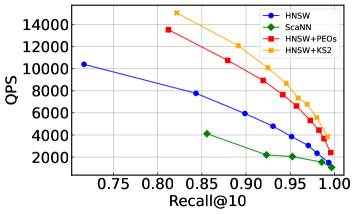
(a) SIFT-$\ell_{2}$

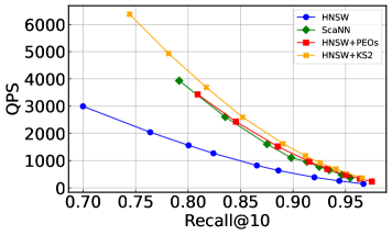
(b) GloVe1M-angular

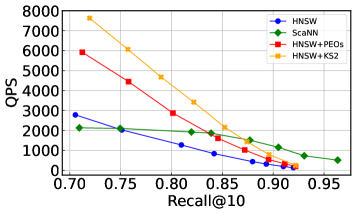
(c) Word-$\ell_{2}$

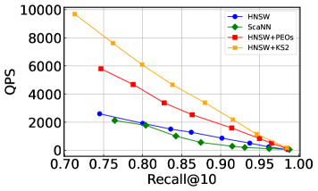
(d) GloVe2M-angular

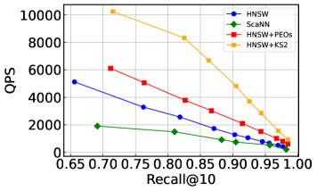
(e) Tiny-$\ell_{2}$

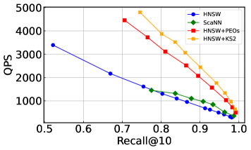
(f) GIST-$\ell_{2}$

Figure 1: Recall-QPS evaluation of ANNS. $k$ = 10.

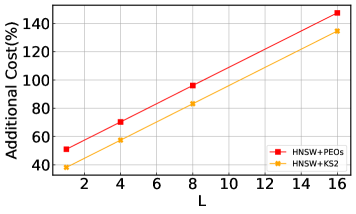
(a) SIFT-$\ell_{2}$

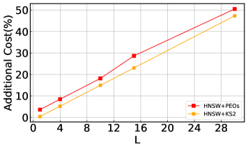
(b) Word-$\ell_{2}$

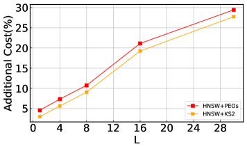
(c) GIST-$\ell_{2}$

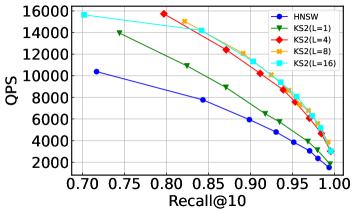
(d) SIFT-$\ell_{2}$

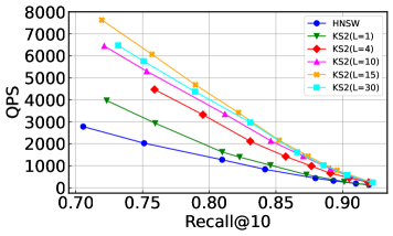
(e) Word-$\ell_{2}$

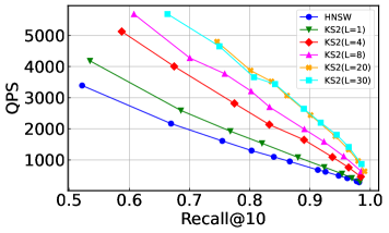
(f) GIST-$\ell_{2}$

Figure 2: Impact of $L$ (See Appendix C.4 for other datasets). $k$ = 10. The y-axis of the upper figures denotes the additional index cost (%) of HNSW+PEOs compared to the original HNSW.

6 Conclusions

In this paper, we studied two angle-testing problems in high-dimensional Euclidean spaces: angle comparison and angle thresholding. To address these problems, we proposed two probabilistic kernel functions that are based on reference angles and are easy to implement. To minimize the reference angle, we further investigated the structure of the projection vectors and established a relationship between the expected value of the reference angle and the proposed projection vector structure. Based on these two functions, we introduced the KS1 projection and the KS2 test. In the experiments, we showed that KS1 achieves a slight accuracy improvement over CEOs, and that HNSW+KS2 delivers better search performance than the existing state-of-the-art ANNS approaches.

Appendix A Proof of Lemmas

A.1 Proof of Lemma 3.2

Proof: (1) For the first statement, due to the existence of random rotation matrix $H$ and symmetry, we only need to prove the following claim:

Claim: Let $\bm{q}$ and $\bm{v}$ be two vectors on $\mathbb{S}^{d-1}$ such that the angle between $\bm{q}$ and $\bm{v}$ is $\phi$. Let $C$ be a spherical cross-section defined as follows.

$$C=\{\bm{u}\in\mathbb{S}^{d-1}:\langle\bm{u},\bm{q}\rangle=\cos\psi\}.$$ (11)

If $u$ is a vector randomly drawn from $C$, the CDF of $\left\langle\bm{v},\bm{u}\right\rangle$ is $I_{t}(\frac{d-2}{2},\frac{d-2}{2})$, where $t=\frac{1}{2}+\frac{x-\cos\phi\cos\psi}{2\sin\phi\sin\psi}$.

Proof of Claim: Without loss of generality, we can rotate the coordinate system so that

$$\bm{q}=(1,0,\cdots,0)\in\mathbb{R}^{d}.$$ (12)

Then, by the definition of $\bm{u}$, $\bm{u}$ can be written as follows

$$\bm{u}=(\cos\psi,\sin\psi\cdot\bm{\omega})$$ (13)

where $\bm{\omega}\in\mathbb{S}^{d-2}\in\mathbb{R}^{d-1}$ is a unit vector in the subspace orthogonal to $\bm{q}$. Similarly, $\bm{v}$ can be expressed as follows.

$$\bm{v}=(\cos\phi,\sin\phi\cdot\bm{\eta})$$ (14)

where $\bm{\eta}\in\mathbb{S}^{d-2}$ is fixed and corresponds to the projection of $\bm{v}$ onto the orthogonal subspace of $\bm{q}$. Then $\left\langle\bm{v},\bm{u}\right\rangle$ can be written as follows.

$$X:=\left\langle\bm{v},\bm{u}\right\rangle=\cos\phi\cos\psi+\sin\phi\sin\psi\cdot W$$ (15)

where $W=\langle\bm{\omega},\bm{\eta}\rangle$ is a random variable. A well-known fact says that $W$ is related to the Beta distribution as follows.

$$T=\frac{W+1}{2}\sim\text{Beta}\left(\frac{d-2}{2},\frac{d-2}{2}\right).$$ (16)

Therefore, we have

$$F_{X}(x)=\mathbb{P}(X\leq x)=\mathbb{P}(T\leq\frac{1}{2}+\frac{x-\cos\phi\cos\psi}{2\sin\phi\sin\psi}).$$ (17)

Thus, $F_{X}(x)=I_{t}(\frac{d-2}{2},\frac{d-2}{2})$, where $t=\frac{1}{2}+\frac{x-\cos\phi\cos\psi}{2\sin\phi\sin\psi}$.

(2) For the second statement, due to the existence of random rotation matrix $H$ and symmetry, we only need to prove the following claim.

Claim: Given three normalized vectors $\bm{v_{1}}$, $\bm{v_{2}}$ and $\bm{q}$, let $\left\langle\bm{q},\bm{v_{1}}\right\rangle$ be larger than $\left\langle\bm{q},\bm{v_{2}}\right\rangle$. Let $C$ be the spherical cross-section defined in the proof of statement 1, and let $\bm{u}$ be a normalized vector drawn randomly from $C$. As $\psi$ decreases, $\mathbb{P}[\left\langle\bm{u},\bm{v_{1}}\right\rangle>\left\langle\bm{u},\bm{v_{2}}\right\rangle]$ increases.

Proof of Claim: For $\bm{u}=\cos\psi\cdot\bm{q}+\sin\psi\cdot\bm{\omega^{\prime}}$, where $\bm{\omega^{\prime}}$ is a random normalized vector, taking $\bm{u}$’s inner products with $\bm{v_{1}}$ and $\bm{v_{2}}$, we obtain:

$$\left\langle\bm{v_{1}},\bm{u}\right\rangle=\cos\psi\left\langle\bm{v_{1}},\bm{q}\right\rangle+\sin\psi\left\langle\bm{v_{1}},\bm{\omega^{\prime}}\right\rangle.$$ (18)

$$\left\langle\bm{v_{2}},\bm{u}\right\rangle=\cos\psi\left\langle\bm{v_{2}},\bm{q}\right\rangle+\sin\psi\left\langle\bm{v_{2}},\bm{\omega^{\prime}}\right\rangle.$$ (19)

Then, we have

$$\mathbb{P}[\left\langle\bm{u},\bm{v_{1}}\right\rangle>\left\langle\bm{u},\bm{v_{2}}\right\rangle]\Leftrightarrow\mathbb{P}[\left\langle\bm{v_{1}},\bm{\omega^{\prime}}\right\rangle-\left\langle\bm{v_{2}},\bm{\omega^{\prime}}\right\rangle>\Delta_{q}\cot\psi]$$ (20)

where $\Delta_{q}=\left\langle\bm{v_{2}},\bm{q}\right\rangle-\left\langle\bm{v_{1}},\bm{q}\right\rangle<0$ and the threshold $\Delta_{q}\cot\psi$ is naturally set to 0 when $\psi=\pi/2$. As $\psi$ decreases, $\cot\psi$ increases, making $\Delta_{q}\cot\psi$ smaller. Since $\left\langle\bm{v_{1}},\bm{\omega^{\prime}}\right\rangle-\left\langle\bm{v_{2}},\bm{\omega^{\prime}}\right\rangle$ is a random variable due to the existence of $\bm{\omega^{\prime}}$, the probability that it exceeds a given threshold increases as the threshold decreases. Thus, as $\psi$ decreases, the probability that the above inequality holds increases.

A.2 Proof of Lemma 3.3

We consider the following four cases based on the value of $\cos\left\langle\bm{q},\bm{v}\right\rangle$.

Case 1: $\bm{0<\cos\left\langle q,v\right\rangle<1}$.

Let $\bm{u}$ be a random vector drawn randomly from a spherical cross-section $C^{\prime}$ defined as follows.

$$C^{\prime}=\{\bm{u}\in\mathbb{S}^{d-1}:\langle\bm{u},\bm{v}\rangle=\cos\psi\}.$$ (21)

Next, we construct a simplex with vertices $O,A,B,C$ as follows. We use $\overrightarrow{OA}$ to denote vector $\bm{v}$, where $O$ denotes the origin. Then we can build a unique hyperplane $H^{\prime}$ through point $A$ and perpendicular to $\bm{v}$. we extend $\bm{q}$ and $\bm{u}$ along their respective directions to $\overrightarrow{OB}$ and $\overrightarrow{OC}$ such that $B$ and $C$ are on $H^{\prime}$. Then, we only need to prove the following claim.

Claim: Let $O,A,B,C$ be four points $\mathbb{R}^{d}$. $\overrightarrow{OA}$ is perpendicular to $\overrightarrow{AB}$, and $\overrightarrow{OA}$ is perpendicular to $\overrightarrow{AC}$. The angle between $\overrightarrow{OA}$ and $\overrightarrow{OC}$ is $\psi$, and the angle between $\overrightarrow{OA}$ and $\overrightarrow{OB}$ is $\phi$. If the angle between $\overrightarrow{AB}$ and $\overrightarrow{AC}$ is $\alpha$, then $\cos\beta$, where $\beta$ denotes the angle between $\overrightarrow{OB}$ and $\overrightarrow{OC}$, can be expressed as follows.

$$\cos\beta=\cos\phi\cos\psi+\sin\phi\sin\psi\cos\alpha.$$ (22)

This claim can be easily proved by elementary transformations. Since $\overrightarrow{AB}$ is fixed and $\overrightarrow{AC}$ follows the uniform distribution of a sphere in $\mathbb{R}^{d-1}$, $\cos\alpha$ and $\cos\beta$ are random variables. Therefore, we have the following equalities.

$$\mathbb{P}[K^{2}_{S}(\bm{q},\bm{v})\geq\cos\theta] =\mathbb{P}[\cos\beta\geq\cos\theta\cos\psi]$$

$$=\mathbb{P}[\cos\alpha\geq\frac{\cos\theta-\cos\phi}{\sin\phi\tan\psi}].$$ (23)

We further consider the following two cases.

Case 1’: $\bm{\cos\phi\geq\cos\theta}$.

$$\mathbb{P}[K^{2}_{S}(\bm{q},\bm{v})\geq\cos\theta]\geq\mathbb{P}[\cos\alpha\geq 0]=1/2.$$ (24)

Case 2’: $\bm{\cos\phi<\cos\theta}$.

By the properties of Beta distribution discussed in the proof of Lemma 3.2 and the property of symmetry of incomplete regularized Beta function, we have

$$\mathbb{P}[K^{2}_{S}(\bm{q},\bm{v})\geq\cos\theta]=I_{t^{\prime}}(\frac{d-2}{2},\frac{d-2}{2})$$ (25)

where $t^{\prime}=\frac{1}{2}-\frac{\cos\theta-\cos\phi}{2\sin\phi\tan\psi}$. Moreover, since $\tan\psi$ is strictly increasing in $\psi$ when $\psi\in(0,\frac{\pi}{2})$, $\mathbb{P}[K^{2}_{S}(\bm{q},\bm{v})\geq\cos\theta]$ is increasing in $\psi$. On the other hand, it is easy to see that $\mathbb{P}[K^{2}_{S}(\bm{q},\bm{v})\geq\cos\theta]$ is strictly decreasing in $\phi$ when $\phi\in(\theta,\pi)$. Hence, Lemma 3.3 in Case 1 is proved.

Case 2: $\bm{\cos\left\langle q,v\right\rangle=0}$.

In this case, without loss of generality, we can define $\bm{q},\bm{v},\bm{u}$ as follows.

$$\bm{q}=(0,1,\cdots,0)\in\mathbb{S}^{d-1}.$$ (26)

$$\bm{v}=(1,0,\cdots,0)\in\mathbb{S}^{d-1}.$$ (27)

$$\bm{u}=(\cos\psi,\sin\psi\cdot\bm{\omega})\in\mathbb{S}^{d-1}\qquad\bm{\omega}\sim U(\mathbb{S}^{d-2}).$$ (28)

Therefore, we have

$$\mathbb{P}[K^{2}_{S}(\bm{q},\bm{v})\geq\cos\theta]=\mathbb{P}[\cos\alpha\geq\cos\theta/\tan\psi]$$ (29)

which is consistent with $\phi=\pi/2$ in Case 1. The following analysis is similar to that in Case 1.

Case 3: $\bm{-1<\cos\left\langle q,v\right\rangle<0}$.

Instead of $\bm{v}$ and $\bm{u}$, we consider $-\bm{v}$ and $-\bm{u}$, and construct the simplex based on $\bm{q}$, $\bm{-v}$ and $\bm{-u}$ as in Case 1. Then, with the reverse of sign, we finally obtain an equation similar to eq. (22), except with $\alpha$ replaced by $\pi-\alpha$. The following analysis is similar to that of Case 1.

Case 4: $\bm{\cos\left\langle q,v\right\rangle=1}$ or $\bm{\cos\left\langle q,v\right\rangle=-1}$.

In this case, $\cos\left\langle\bm{q},\bm{u}\right\rangle=\pm\cos\psi$, and the conclusion is trivial.

A.3 Proof of Lemma 3.4

Before proving this theorem, we first introduce a uniformly distributed sequence.

Definition A.1

(Uniformly distributed sequence) A sequence $\{w_{N}\}^{\infty}_{N=2}$ of $N$-point configuration on $\mathbb{S}^{d-1}$ is called uniformly distributed if for every closed subset $B\in\mathbb{S}^{d-1}$ whose boundary relative to $\mathbb{S}^{d-1}$ has $d$-dimensional measure zero,

$$\lim_{N\to\infty}\frac{\#(\omega_{N}\cap B)}{N}=\sigma_{d}(B)$$ (30)

where $\sigma_{d}(B)$ is the area measure on $\mathbb{S}^{d-1}$ normalized to a probability measure.

Proof Let $\{v_{i,N}\}^{N}_{i=1}\subset\mathbb{S}^{d-1}$ be an i.i.d. sequence drawn from the uniform distribution $\sigma_{d}$, i.e., the area measure on $\mathbb{S}^{d-1}$ normalized to be a probability measure, and let $w_{N}=\{v_{1,N},v_{2,N}\ldots v_{N,N}\}$.

By SLLN, we have

$$\frac{1}{N}\sum_{i=1}^{N}\mathbf{1}_{B}(v_{i,N})\xrightarrow{\text{a.s.}}\mathbb{E}[\mathbf{1}_{B}(v_{1,N})]=\sigma_{d}(B).$$ (31)

$$\mathbb{P}\left[\lim_{N\to\infty}\frac{\#(\omega_{N}\cap B)}{N}=\sigma_{d}(B)\right]=1.$$ (32)

On the other hand, the sequence $\{w_{N}\}^{\infty}_{N=2}$ is uniformly distributed on $\mathbb{S}^{d-1}$ if and only if, for every continuous function $f:\mathbb{S}^{d-1}\rightarrow\mathbb{R}$, we have

$$\frac{1}{N}\sum_{i=1}^{N}f(v_{i,N})\rightarrow\int_{\mathbb{S}^{d-1}}f(v)\,\mathrm{d}\sigma_{d}(v),\quad N\rightarrow\infty.$$ (33)

Define $f(v)$ as follows

$$f(v)=\cos\left\langle\bm{v},Z_{S}(\bm{v})\right\rangle.$$ (34)

Clearly, $f(v)$ is a continuous function w.r.t $v$. if we substitute $f(v)$ into relationship (33), the lemma is proved.

Algorithm 3 Configuration of $S$ via random projection

Input: $L$ is the level; $d=Ld^{\prime}$ is the data dimension; $m$ is the number of vectors in each level

Output: $S_{\text{ran}}(m,L)$, which is physically represented by $mL$ sub-vectors with dimension $d^{\prime}$

for $l=1$ to $L$ do

12    Generate $m$ points randomly and independently on $S^{d^{\prime}-1}$  Scale the norm of all $m$ points in this iteration to $1/\sqrt{L}$ and collect the vectors after scaling 

A.4 Proof of Lemma 3.5

Proof: First, we introduce an auxiliary algorithm Alg. 3, which relies on purely random projection. The structure $S$ produced in Alg. 3 is denoted by $S_{\text{ran}}$. We then present the following claim.

Claim: $J(S_{\text{sym}}(m,L))>J(S_{\text{ran}}(m,L))$.

To prove this claim, we introduce the following definition.

Definition A.2

(Stochastic order) Let $X$ and $Y$ be two real-valued random variables. We say that $X<_{st}Y$, if for all $t\in\mathbb{R}$, the CDFs of $X$ and $Y$ satisfy $F_{X}(t)>F_{Y}(t)$.

Let $L=1$ and fix $m$. We use $X$ to denote the random variable $A_{S_{\text{ran}}}(\bm{v})$, where $\bm{v}$ is drawn randomly from $\mathbb{S}^{d-1}$, and $Y$ to denote $A_{S_{\text{sym}}}(\bm{v})$. Clearly, $X\in[-1,1]$ and $Y\in[0,1]$. We have the following:

$$\mathbb{P}(Y>t)>\mathbb{P}(X>t)\quad t\in(0,1).$$ (35)

This can be easily proved, since when the angular radius is less than $\pi/2$, the two spherical caps corresponding to the antipodal pair do not overlap. Therefore, we have $X<_{st}Y$ and $\mathbb{E}[X]<\mathbb{E}[Y]$. This completes the proof of the claim.

Then we only need to focus on $J(S_{\text{ran}}(m,L))$ and prove that it is equal to the RHS of ineq. (8). Let $\bm{v=[v_{1},v_{2},\cdots.v_{L}]}\in\mathbb{R}^{n}$ be a vector drawn randomly from $\mathbb{S}^{d-1}$, where $d$ is assumed to be divisible by $L$ and $d=Ld^{\prime}$. Let $r_{L}(\bm{v})$ be the regularized vector w.r.t. $\bm{v}$. That is,

$$r_{L}(\bm{v})=[\frac{\bm{v_{1}}}{\sqrt{L}\|\bm{v_{1}}\|},\frac{\bm{v_{2}}}{\sqrt{L}\|\bm{v_{2}}\|},\ldots,\frac{\bm{v_{L}}}{\sqrt{L}\|\bm{v_{L}}\|}].$$ (36)

Let $T(d,L)=\cos\left\langle\bm{v},r_{L}(\bm{v})\right\rangle$. For every $i$, let $\bm{u_{i}}=\bm{v_{i}}/\|\bm{v_{i}}\|\in\mathbb{S}^{d^{\prime}-1}$. Then we select $m$ vectors from $\mathbb{S}^{d^{\prime}-1}$ randomly and independently. Suppose that, among $m$ generated vectors, $\bm{w}$ is the vector having the smallest angle to $\bm{u_{i}}$, and we use $T^{\prime}(d^{\prime},L)$ to denote $\cos\left\langle\bm{w},\bm{u_{i}}\right\rangle$. Since the choice of $w$ for every $u_{i}$ is independent to the value of $\cos\left\langle\bm{v},r_{L}(\bm{v})\right\rangle$, we have the following result:

$$\mathbb{E}[A_{S}(\bm{v})]=\mathbb{E}[T(d,L)]\times\mathbb{E}[T^{\prime}(d^{\prime},L)].$$ (37)

For $\mathbb{E}[T(d,L)]$, since $(\|\bm{v_{1}}\|^{2},\|\bm{v_{2}}\|^{2},\ldots,\|\bm{v_{L}}\|^{2})$ follows a Dirichlet distribution with parameters $(\frac{d}{2L},\frac{d}{2L},\ldots,\frac{d}{2L})$, each $\|\bm{v_{i}}\|^{2}$ marginally follows a Beta distribution with parameters $(\frac{d}{2L},\frac{d(L-1)}{2L})$. Then by the properties of Beta distribution, we have

$$E[T(d,L)]=\sqrt{L}\frac{\Gamma(\frac{d+L}{2L})\Gamma(\frac{d}{2})}{\Gamma(\frac{d}{2L})\Gamma(\frac{d+1}{2})}.$$ (38)

Next, we consider $\mathbb{E}[T^{\prime}(d^{\prime},L)]$. Because of the rotational symmetry of the sphere, the distribution of the inner product $Z=\langle u,v\rangle$ (for fixed $v$ and uniformly random $u$) depends only on the dimension $d^{\prime}$. It has the following density on $[-1,1]$:

$$f_{Z}(z)=c_{d^{\prime}}(1-z^{2})^{\frac{d^{\prime}-3}{2}}$$ (39)

where $c_{d^{\prime}}$ is defined as follows.

$$c_{d^{\prime}}=\frac{\Gamma\left(\frac{d^{\prime}}{2}\right)}{\sqrt{\pi}\,\Gamma\left(\frac{d^{\prime}-1}{2}\right)}.$$ (40)

Let $Z_{1},\dots,Z_{n}$ be i.i.d. copies of $Z=\langle u,v\rangle$. Then:

$$Y=\max(Z_{1},\dots,Z_{m}).$$ (41)

The cumulative distribution function (CDF) of $Z$ is:

$$F_{Z}(z)=\int_{-1}^{z}f_{Z}(t)\,\mathrm{d}t.$$ (42)

Thus, the CDF of $Y=Y(d^{\prime},m)$ is:

$$F_{Y}(y)=\mathbb{P}(Y\leq y)=F_{Z}(y)^{m},$$ (43)

and the corresponding density is:

$$f_{Y}(y)=\frac{\mathrm{d}}{\mathrm{d}y}F_{Z}(y)^{m}=mF_{Z}(y)^{m-1}f_{Z}(y).$$ (44)

Therefore, we have the following result.

$$\mathbb{E}[Y]=\int_{-1}^{1}yf_{Y}(y)\,\mathrm{d}y=m\int_{-1}^{1}yF_{Z}(y)^{m-1}f_{Z}(y)\,\mathrm{d}y.$$ (45)

Combining the previous results, we get the following result.

$$J(S_{\text{ran}}(m,L))=m\sqrt{L}\frac{\Gamma(\frac{d+L}{2L})\Gamma(\frac{d}{2})}{\Gamma(\frac{d}{2L})\Gamma(\frac{d+1}{2})}\int_{-1}^{1}yF_{Z}(y)^{m-1}f_{Z}(y)\,\mathrm{d}y.$$ (46)

Appendix B Supplementary Materials

B.1 Illustration of Random Projection Techniques for Angle Estimation

An illustration is shown in Fig. 3. In this figure, $\bm{q}$ represents a query and $\bm{v}$ is a data vector. For Falconn, if $\bm{q}$ and $\bm{v}$ are mapped to the same vector, they are considered close. For CEOs and KS1, the inner product $\bm{v}^{\top}\bm{u}$, where $\bm{u}$ is the projection vector closest to $\bm{q}$, is computed to obtain a more accurate estimate of $\bm{q}^{\top}\bm{v}$. The key difference between CEOs and KS1 lies in the structure of the projection vectors. While CEOs uses projection vectors sampled from a Gaussian distribution, KS1 employs a more balanced structure in which all projection vectors lie on the surface of a sphere. By applying a random rotation matrix and constructing a spherical cross-section centered at $\bm{q}$, we can establish the required statistical relationship between $\bm{q}^{\top}\bm{u}$ and $\bm{q}^{\top}\bm{v}$.

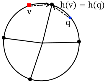
(a) Falconn

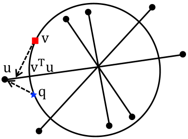
(b) CEOs (Falconn++)

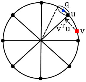
(c) KS1 (proposed one)

Figure 3: An illustration of Falconn, CEOs, and the proposed structure KS1.

B.2 ANNS and Similarity Graphs

As one of the most fundamental problems, approximate nearest neighbor search (ANNS) has seen a surge of interest in recent years, leading to the development of numerous approaches across different paradigms. These include tree-based methods [10], hashing-based methods [3, 20, 1, 4, 26], vector quantization (VQ)-based methods [19, 15, 5, 16], learning-based methods [17, 21], and graph-based methods [23, 27, 14, 13].

Among these, graph-based methods are widely regarded as the state-of-the-art. Currently, three main types of optimizations are used to enhance their search performance: (1) improved edge-selection strategies, (2) more effective routing techniques, and (3) quantization of raw vectors. These approaches are generally orthogonal to one another. Since the proposed structure, PEOs, belongs to the second category, we briefly introduce several highly relevant works below. TOGG-KMC[29] and HCNNG[24] use KD-trees to determine the direction of the query and restrict the search to points in that direction. While this estimation is computationally efficient, it results in relatively low query accuracy, limiting their improvements over HNSW[23]. FINGER[9] examines all neighbors and estimates their distances to the query. Specifically, for each node, FINGER locally generates promising projection vectors to define a subspace, then uses collision counting which is similar to SimHash to approximate distances within each visited subspace. Learn-to-Route [6] learns a routing function using auxiliary representations that guide optimal navigation from the starting vertex to the nearest neighbor. Recently, the authors of [22] proposed PEOs, which leverages space partitioning and random projection techniques to estimate a random variable representing the angle between each neighbor and the query vector. By aggregating projection information from multiple subspaces, PEOs substantially reduces the variance of this estimated distribution, significantly improving query accuracy.

B.3 Algorithms Related to KS1 and KS2

Alg. 4 and Alg. 5 are used to compare the probing accuracies of CEOs and KS1, while Alg. 6 presents the graph-based search equipped with the KS2 test.

Algorithm 4 Construction of the Projection Structure of KS1

Input: $\mathcal{D}$ is the dataset with cardinality $n$, and $S$ is the configuration of $m$ projection vectors (CEOs: $m/2$ random Gaussian vectors along with their antipodal vectors; KS1: $S_{\text{sym}}(m,1)$ or $S_{\text{pol}}(m,1)$)

Output: $m$ projection vectors, each of which is associated with a $n$-sequence of data ID’s

For every $x_{i}\in\mathcal{D}$ ($1\leq i\leq n$) and each $u_{j}\in S$ ($1\leq j\leq m$), compute $\left\langle\bm{x_{i}},\bm{u_{j}}\right\rangle$

For each $u_{j}\in S$, sort $x_{i}$ in descending order of $\left\langle\bm{x_{i}},\bm{u_{j}}\right\rangle$ and obtain $x^{j}_{[1]},\ldots x^{j}_{[n]}$

Algorithm 5 Query Phase for MIPS

Input: $q$ is the query; $\mathcal{D}$ is the dataset; $\mathcal{I}$ is the index structure returned by Alg. 4; $k$ denotes the value of top-$k$; $s_{0}$ is the number of scanned top projection vectors; and #probe denotes the number of probed points for each projection vector

Output: Top-$k$ MIP results of $q$

Among the $m$ projection vectors, find the top-$s_{0}$ projection vectors closest to $q$

For each projection vector $u_{l}$ in the top-$s_{0}$ set ($1\leq l\leq s_{0}$), scan the top-#probe points in the sequence associated with $u_{l}$, and compute the exact inner products of these points with $q$

Maintain and return the top-$k$ points among all scanned candidates

Algorithm 6 Graph-based ANNS with the KS2 test

Input :

$\bm{q}$ is the query, $k$ denotes the value of top-$k$, $G$ is the graph index

Output :

Top-$k$ ANNS results of $q$

$R\leftarrow\emptyset$ ;

  /* an ordered list of results, $|R|\leq efs$ */ $P\leftarrow\{\,$ entry node $v_{0}\in G\,\}$ ;

13  /* a priority queue */ while $P\neq\emptyset$ do

14    $v\leftarrow P.pop()$  foreach unvisited neighbor $w$ of $v$ do

15       if $|R|<efs$ then $\delta\leftarrow\infty$;

16       else $v^{\prime}\leftarrow R[efs]$, $\delta\leftarrow dist(\bm{v^{\prime}},\bm{q})$;

17       if KS2_Test($\bm{w},\bm{v},\bm{q},\delta$) = true (see ineq. (10)) then

18          if $dist(\bm{w},\bm{q})<\delta$ then

19             $R.push(w)$, $P.push(w)$ 

20         

21      

22   

return ($\{\,R[1],\ldots,R[k]\,\}$)

B.4 Numerical Computation of Reference angle

Fig. 4 shows the numerical values of the lower bounds (the RHS of ineq. (8)) under different pairs of $(m,L)$. From the results, we observe that increasing $L$ significantly raises the cosine of the reference angle, whereas a linear increase in $m$ leads to only a slow growth in the cosine of the reference angle, which explains why we need to introduce parameter $L$ into our projection structure.

Appendix C Additional Experiments

C.1 Datasets and Parameter Settings

Table 2: Dataset statistics.

Dataset	Data Size	Query Size	Dimension	Type	Metric
Word	1,000,000	1,000	300	Text	$\ell_{2}$&inner product
GloVe1M	1,183,514	10,000	200	Text	angular&inner product
GloVe2M	2,196,017	1,000	300	Text	angular&inner product
SIFT	10,000,000	1,000	128	Image	$\ell_{2}$
Tiny	5,000,000	1,000	384	Image	$\ell_{2}$
GIST	1,000,000	1,000	960	Image	$\ell_{2}$

The statistic of six datasets used in this paper is shown in Tab. 2. The parameter settings of all compared methods are shown as follows.

(1) CEOs: The number of projection vectors, $m$, was set to 2048, following the standard setting in the original paper [25].

(2) KS1: For KS1, $L$ was fixed to 1, as multiple levels are not necessary for angle comparison. The number of projection vectors, $m$, was also set to 2048, consistent with CEOs. We evaluated both KS1($S=S_{\text{sym}}(2048,1)$) and KS1($S=S_{\text{pol}}(2048,1)$).

(3) HNSW: $M$ was set to 32. The parameter efc was set to 1000 for SIFT, Tiny, and GIST, and to 2000 for Word, GloVe1M, and GloVe2M.

(4) ScaNN: The Dimensions_per_block was set to 4 for Tiny and GIST, and to 2 for the other datasets. num_leaves was set to 2000. The other user-specified parameters were tuned to achieve the best trade-off curves.

(5) HNSW+PEOs: Following the suggestions in [22], we set $L$ to 8, 10, 15, 15, 16, and 20 for the six real datasets, sorted in ascending order of dimension. Additionally, $\epsilon$ was set to 0.2, and $m=256$ to ensure that each vector ID could be encoded with a single byte.

(6) HNSW+KS2: $S$ was fixed to $S_{\text{sym}}(m,L)$. The only tunable parameter is $L$, as $m$ must be fixed at 256 to ensure that each vector ID is encoded with a single byte. Since the parameter $L$ in KS2 plays a similar role to that in PEOs, we set $L$ to the same value in HNSW+PEOs to eliminate the influence of $L$ in the comparison.

C.2 KS1 vs. CEOs under Different Settings

In Tab. 1, we compared the performance of CEOs and KS1 using the top-5 probed projection vectors. Here, we varied the value of $s_{0}$ in Alg. 5 from 5 to 2 and 10, and present the corresponding results in Tab. 3 and Tab. 4, respectively. We observe that KS1($S_{\text{pol}}$) still achieves the highest probing accuracy in most cases.

C.3 ANNS Results under Different $k$’s

Fig. 5 and Fig. 6 show the comparison results of ANNS solvers under different values of $k$. When $k=1$, ScaNN performs very well on Word, GloVe1M, GloVe2M, and Tiny, which is partly due to the connectivity issue of HNSW on these datasets. In the other cases, HNSW+KS2 achieves the best performance.

C.4 The Impact of $L$ on the Other Datasets

Fig. 7 shows the impact of $L$ on GloVe1M, GloVe2M, and Tiny, which is largely consistent with the results in Fig. 2.

C.5 Results of NSSG+KS2

We also implement KS2 on another state-of-the-art similarity graph, NSSG [13]. The parameter settings for NSSG are the same as those in [22]. From the results in Fig. 8, we observe that NSSG+KS2 outperforms NSSG+PEOs on all datasets except for GIST, which indicates that the superiority of KS2 is independent of the underlying graph structure.

Table 3: Comparison of recall rates (%) for $k$-MIPS, $k$ = 10. Top-2 projection vectors are probed.

Dataset & Method		Probe@10	Probe@100	Probe@1K	Probe@10K
Word	CEOs(2048)	17.255	46.348	68.893	84.366
	KS1($S_{\text{ran}}(2048,1)$)	17.334	46.740	69.232	84.548
	KS1($S_{\text{act}}(2048,1)$)	17.440	46.843	69.392	85.026
GloVe1M	CEOs(2048)	0.839	3.404	12.694	38.607
	KS1($S_{\text{ran}}(2048,1)$)	0.849	3.464	12.890	39.109
	KS1($S_{\text{act}}(2048,1)$)	0.866	3.503	12.916	39.170
GloVe2M	CEOs(2048)	0.934	3.407	11.621	34.917
	KS1($S_{\text{ran}}(2048,1)$)	0.939	3.451	11.775	35.462
	KS1($S_{\text{act}}(2048,1)$)	0.917	3.401	11.748	35.159

Table 4: Comparison of recall rates (%) for $k$-MIPS, $k$ = 10. Top-10 projection vectors are probed.

Dataset & Method		Probe@10	Probe@100	Probe@1K	Probe@10K
Word	CEOs(2048)	50.772	84.545	96.620	99.882
	KS1($S_{\text{ran}}(2048,1)$)	50.698	84.470	96.643	99.869
	KS1($S_{\text{act}}(2048,1)$)	51.238	84.865	96.869	99.910
GloVe1M	CEOs(2048)	3.012	11.301	36.293	80.995
	KS1($S_{\text{ran}}(2048,1)$)	3.047	11.401	36.604	81.307
	KS1($S_{\text{act}}(2048,1)$)	3.069	11.451	36.857	81.781
GloVe2M	CEOs(2048)	3.574	11.252	30.695	69.406
	KS1($S_{\text{ran}}(2048,1)$)	3.567	11.256	30.741	69.668
	KS1($S_{\text{act}}(2048,1)$)	3.515	11.368	30.940	70.016

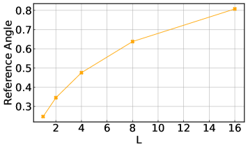
(a) Dim=128, $m=256$

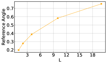
(b) Dim=200, $m=256$

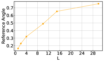
(c) Dim=300, $m=256$

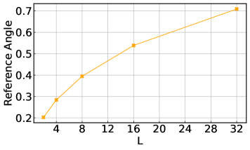
(d) Dim=384, $m=256$

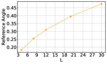
(e) Dim=960, $m=256$

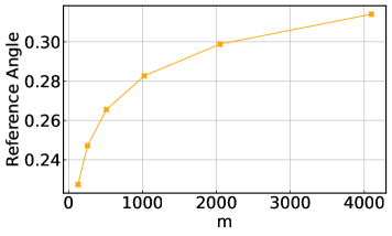
(f) Dim=128, $L=1$

Figure 4: Numerical computation under different $m$’s and $d$’s. The y-axis denotes the cosine of reference angle.

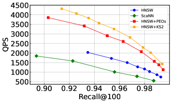
(a) SIFT-$\ell_{2}$

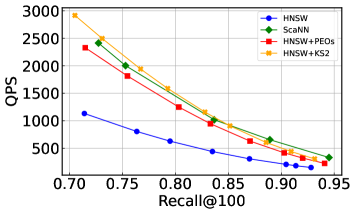
(b) GloVe1M-angular

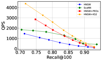
(c) Word-$\ell_{2}$

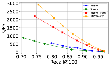
(d) GloVe2M-angular

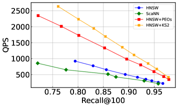
(e) Tiny-$\ell_{2}$

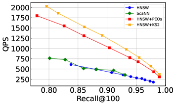
(f) GIST-$\ell_{2}$

Figure 5: Recall-QPS evaluation of ANNS. $k$ = 100.

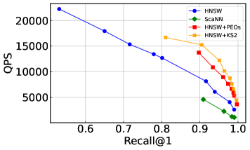
(a) SIFT-$\ell_{2}$

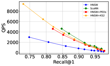
(b) GloVe1M-angular

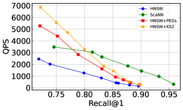
(c) Word-$\ell_{2}$

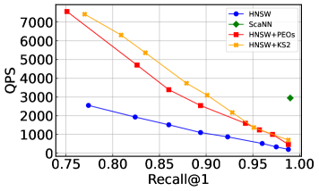
(d) GloVe2M-angular

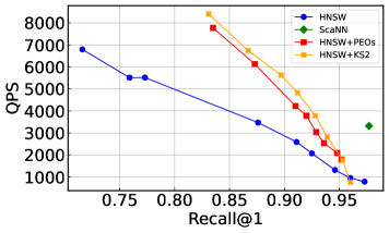
(e) Tiny-$\ell_{2}$

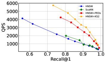
(f) GIST-$\ell_{2}$

Figure 6: Recall-QPS evaluation of ANNS. $k$ = 1.

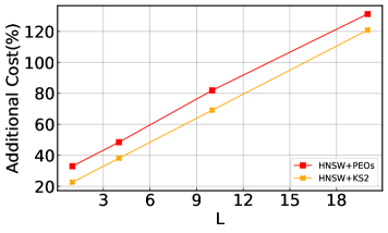
(a) GloVe1M-angular

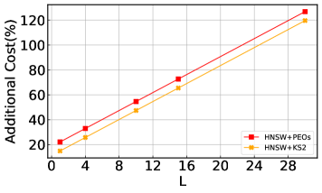
(b) GloVe2M-angular

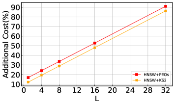
(c) Tiny-$\ell_{2}$

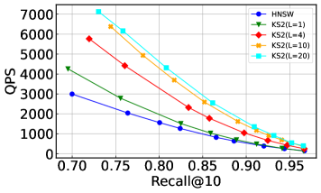
(d) GloVe1M-angular

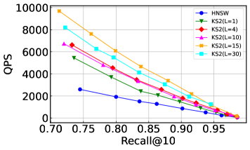
(e) GloVe2M-angular

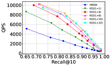
(f) Tiny-$\ell_{2}$

Figure 7: Impact of $L$ on index sizes and search performance. $k$ = 10.

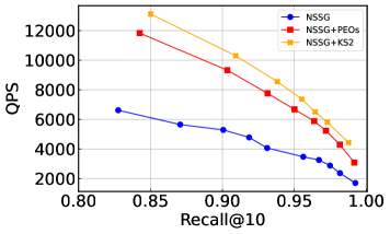
(a) SIFT-$\ell_{2}$

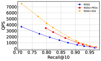
(b) GloVe1M-angular

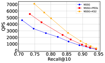
(c) Word-$\ell_{2}$

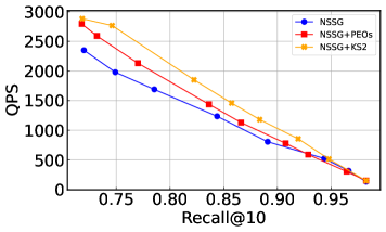
(d) GloVe2M-angular

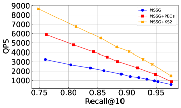
(e) Tiny-$\ell_{2}$

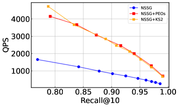
(f) GIST-$\ell_{2}$

Figure 8: Recall-QPS evaluation of ANNS, with NSSG+KS2. $k$ = 10.

References

- (1) Alexandr Andoni and Daniel Beaglehole. Learning to hash robustly, guaranteed. In ICML, pages 599–618, 2022.
- (2) Alexandr Andoni and Piotr Indyk. E2lsh manual. In http://web.mit.edu/andoni/www/LSH.
- (3) Alexandr Andoni and Piotr Indyk. Near-optimal hashing algorithms for approximate nearest neighbor in high dimensions. Commun. ACM, 51(1):117–122, 2008.
- (4) Alexandr Andoni, Piotr Indyk, Thijs Laarhoven, Ilya P. Razenshteyn, and Ludwig Schmidt. Practical and optimal LSH for angular distance. In NeurIPS, pages 1225–1233, 2015.
- (5) Artem Babenko and Victor S. Lempitsky. Efficient indexing of billion-scale datasets of deep descriptors. In CVPR, pages 2055–2063, 2016.
- (6) Dmitry Baranchuk, Dmitry Persiyanov, Anton Sinitsin, and Artem Babenko. Learning to route in similarity graphs. In ICML, pages 475–484, 2019.
- (7) Sergiy Borodachov. Optimal antipodal configuration of 2d points on a sphere in rd for coverings. In arxiv, 2022.
- (8) Moses Charikar. Similarity estimation techniques from rounding algorithms. In John H. Reif, editor, STOC, pages 380–388. ACM, 2002.
- (9) Patrick H. Chen, Wei-Cheng Chang, Jyun-Yu Jiang, Hsiang-Fu Yu, Inderjit S. Dhillon, and Cho-Jui Hsieh. FINGER: fast inference for graph-based approximate nearest neighbor search. In WWW, pages 3225–3235. ACM, 2023.
- (10) Ryan R. Curtin, Parikshit Ram, and Alexander G. Gray. Fast exact max-kernel search. Statistical Analysis and Data Mining, 7(1):1–9, February–December 2014.
- (11) Xinyan Dai, Xiao Yan, Kelvin Kai Wing Ng, Jiu Liu, and James Cheng. Norm-explicit quantization: Improving vector quantization for maximum inner product search. In AAAI, pages 51–58, 2020.
- (12) Anirban Dasgupta, Ravi Kumar, and Tamás Sarlós. Fast locality-sensitive hashing. In KDD, pages 1073–1081, 2011.
- (13) Cong Fu, Changxu Wang, and Deng Cai. High dimensional similarity search with satellite system graph: Efficiency, scalability, and unindexed query compatibility. IEEE Trans. Pattern Anal. Mach. Intell., 44(8):4139–4150, 2022.
- (14) Cong Fu, Chao Xiang, Changxu Wang, and Deng Cai. Fast approximate nearest neighbor search with the navigating spreading-out graph. PVLDB, 12(5):461–474, 2019.
- (15) Tiezheng Ge, Kaiming He, Qifa Ke, and Jian Sun. Optimized product quantization. IEEE Trans. Pattern Anal. Mach. Intell, 36(4):744–755, 2014.
- (16) Ruiqi Guo, Philip Sun, Erik Lindgren, Quan Geng, David Simcha, Felix Chern, and Sanjiv Kumar. Accelerating large-scale inference with anisotropic vector quantization. In ICML, pages 3887–3896, 2020.
- (17) Gaurav Gupta, Tharun Medini, Anshumali Shrivastava, and Alexander J. Smola. BLISS: A billion scale index using iterative re-partitioning. In KDD, pages 486–495. ACM, 2022.
- (18) Piotr Indyk and Rajeev Motwani. Approximate nearest neighbors: Towards removing the curse of dimensionality. In STOC, pages 604–613, 1998.
- (19) Hervé Jégou, Matthijs Douze, and Cordelia Schmid. Product quantization for nearest neighbor search. IEEE Trans. Pattern Anal. Mach. Intell, 33(1):117–128, 2011.
- (20) Yifan Lei, Qiang Huang, Mohan Kankanhalli, and Anthony Tung. Sublinear time nearest neighbor search over generalized weighted space. In ICML, pages 3773–3781, 2019.
- (21) Wuchao Li, Chao Feng, Defu Lian, Yuxin Xie, Haifeng Liu, Yong Ge, and Enhong Chen. Learning balanced tree indexes for large-scale vector retrieval. In KDD, pages 1353–1362. ACM, 2023.
- (22) Kejing Lu, Chuan Xiao, and Yoshiharu Ishikawa. Probabilistic routing for graph-based approximate nearest neighbor search. In ICML, pages 33177–33195, 2019.
- (23) Yury A. Malkov and D. A. Yashunin. Efficient and robust approximate nearest neighbor search using hierarchical navigable small world graphs. IEEE Trans. Pattern Anal. Mach. Intell, 42(4):824–836, 2020.
- (24) Javier Alvaro Vargas Muñoz, Marcos André Gonçalves, Zanoni Dias, and Ricardo da Silva Torres. Hierarchical clustering-based graphs for large scale approximate nearest neighbor search. Pattern Recognit., 96, 2019.
- (25) Ninh Pham. Simple yet efficient algorithms for maximum inner product search via extreme order statistics. In KDD, pages 1339–1347, 2021.
- (26) Ninh Pham and Tao Liu. Falconn++: A locality-sensitive filtering approach for approximate nearest neighbor search. In NeurIPS, pages 31186–31198, 2022.
- (27) Suhas Jayaram Subramanya, Fnu Devvrit, Harsha Vardhan Simhadri, Ravishankar Krishnaswamy, and Rohan Kadekodi. Rand-nsg: Fast accurate billion-point nearest neighbor search on a single node. In NeurIPS, pages 13748–13758, 2019.
- (28) Haochuan Xu and Ninh Pham. Scalable DBSCAN with random projections. In NeurIPS, 2024.
- (29) Xiaoliang Xu, Mengzhao Wang, Yuxiang Wang, and Dingcheng Ma. Two-stage routing with optimized guided search and greedy algorithm on proximity graph. Knowl. Based Syst., 229:107305, 2021.
- (30) Xiao Yan, Jinfeng Li, Xinyan Dai, Hongzhi Chen, and James Cheng. Norm-ranging LSH for maximum inner product search. In NeurIPS, pages 2956–2965, 2018.