Hardware-tailored logical Clifford circuits for stabilizer codes

Abstract

Quantum error correction is the art of protecting fragile quantum information through suitable encoding and active interventions. After encoding $k$ logical qubits into $n>k$ physical qubits using a stabilizer code, this amounts to measuring stabilizers, decoding syndromes, and applying an appropriate correction. Although quantum information can be protected in this way, it is notoriously difficult to manipulate encoded quantum data without introducing uncorrectable errors. Here, we introduce a mathematical framework for constructing hardware-tailored quantum circuits that implement any desired Clifford unitary on the logical level of any given stabilizer code. Our main contribution is the formulation of this task as a discrete optimization problem. We can explicitly integrate arbitrary hardware connectivity constraints. As a key feature, our framework naturally incorporates an optimization over all Clifford gauges (differing only in their action outside the code space) of a desired logical circuit. In this way, we find, for example, fault-tolerant and teleportation-free logical Hadamard circuits for the $\llbracket 8,3,2\rrbracket$ code. From a broader perspective, we turn away from the standard generator decomposition approach and instead focus on the holistic compilation of entire logical circuits, leading to significant savings in practice. Our work introduces both the necessary mathematics and open-source software to compile hardware-tailored logical Clifford circuits for stabilizer codes.

I Introduction

The anticipated advantage of quantum computers has not yet been fully realized because decoherence and operational errors are still severely limiting their performance. The most promising and at the same time widely accepted solution to overcome this challenge is presented by quantum error-correcting codes (QECCs), in particular, by stabilizer QECCs, which constitute the by far most well-developed framework. Here, a carefully selected set of Pauli operators (the stabilizer generators) is repeatedly measured, thereby pushing the state of the quantum computer back toward the logical subspace Gottesman (1997); Calderbank et al. (1998). While quantum error correction has been a well-established theoretical field for many years, it is only recently that emphasis has shifted toward actually experimentally realizing core elements of stabilizer error correction. For example, the possibility to ever extend the lifetime of a logical qubit by encoding it into more and more physical qubits has been experimentally confirmed Google Quantum AI (2023); Google Quantum AI and collaborators (2025), including real-time decoding with millions of error correction cycles Google Quantum AI and collaborators (2025). Moreover, various logical primitives have been implemented in the laboratory Egan et al. (2021); Erhard et al. (2021); Postler et al. (2022); Bluvstein et al. (2024); Wang et al. (2024); Honciuc Menendez et al. (2024); Lacroix et al. (2024); Burton et al. (2024); Ryan-Anderson et al. (2024); Jin et al. (2025); Yamamoto et al. (2025). With the fundamental principles of error correction thus being established, a remaining challenge in making quantum error correction practical is to lessen the burden arising from the daunting resource demands of logical operations. This issue has to be addressed and tackled from several perspectives. In particular, to this end, sophisticated compilation methods are urgently needed, especially in the form of methods that take experimental constraints such as limited qubit connectivities into account that are relevant for most physical platforms for quantum error correction.

This is, of course, not a new problem. One of the first proposals for universal fault-tolerant quantum computation is surface code lattice surgery Horsman et al. (2012). While its modular approach and conceptual simplicity offer a clear route to large-scale fault-tolerant quantum computers, surface code lattice surgery faces massive resource overheads: (i) the stabilizer generators must be measured increasingly often as the code size increases, which slows down computation, (ii) many of the logical qubits are blocked; both to route the flow of data and to effectively implement logical Clifford gates via parity measurements of logical multi-qubit Pauli operators Litinski (2019), and (iii) it suffers from certain no-go theorems which limit all codes whose stabilizer generators are local in two dimensions Bravyi and Terhal (2009); Bravyi and König (2013).

Recent discoveries of good quantum low-density parity check (qLDPC) codes Bravyi and Hastings (2014); Breuckmann and Eberhardt (2021a); Panteleev and Kalachev (2022); Leverrier and Zémor (2023); Bravyi et al. (2024); Xu et al. (2024) have added an entirely new flavor to the problem. They elegantly circumvent these no-go results by dropping the locality assumption, motivating a rich and promising research program on generalized lattice surgery for qLDPC codes Cohen et al. (2022); Cowtan and Burton (2024); Cowtan (2024); Cross et al. (2024); Williamson and Yoder (2024); Stein et al. (2024); Swaroop et al. (2024); Cowtan et al. (2025); He et al. (2025); Poirson et al. (2025). While these various readings of qLDPC surgery, indeed, bring down the required number of qubits, they unfortunately inherit several drawbacks from its predecessor for the surface code: (i) in order to ensure fault tolerance, stabilizer generators must still be measured multiple times, and (ii) to implement Clifford gates, some logical qubits are blocked. On top of this, an additional quantum co-processor is required, in order to address the logical qubits in a qLDPC memory, which significantly increases the overall number of qubits. Moreover, the size and layout of this co-processor highly depends on the choice of logical Pauli operators whose parities ought to be measured. This, in turn, considerably limits the flexibility of qLDPC surgery and leads to further overheads for routing logical information.

In a different line of research closely related to qLDPC surgery, notions of code deformation Bombin (2011); Vuillot et al. (2019); Brown et al. (2017) were extended to certain qLDPC codes Krishna and Poulin (2021). However, code deformation also relies on Pauli parity measurements and therefore faces similar challenges as qLDPC surgery.

Cheaper alternatives exist in specific settings, with the most efficient protocols being based on transversal implementations of logical gates . Various methods have been proposed for compiling transversal Clifford gates Webster et al. (2023); Quintavalle et al. (2023); Breuckmann and Burton (2024); Sayginel et al. (2025); Malcolm et al. (2025) as well as non-Clifford gates Lin (2024); Hsin et al. (2024). However, the existence of such gates is not guaranteed for all codes, and design trade-offs are often necessary to provide the necessary structure to support transversal implementations.

This discussion highlights an apparent gap between state-of-the-art experiments and theoretical ideas: while theory research seeks general and scalable protocols with provable properties, experimentalists require concrete implementations for specific codes under real hardware constraints. It can take multiple years of developing, fabricating, and calibrating a quantum device before one can execute an error correction experiment. Here, early design choices may limit the possibility of migrating to newly-discovered QECCs with better code parameters or logical gates. Ideally, one would have access to a method that is agnostic to the QECC and, given a target gate and hardware constraints, constructs an implementation of the logical gate with as little overhead as possible. In other words, the task is to decompose a logical operation into a short sequence of physical operations. In this work, we will refer to such a decomposition as a circuit implementation of the logical gate. However, this problem is notoriously difficult, particularly when it comes to fault-tolerant operations.

In this work, we develop a general framework for the synthesis of efficient circuit implementations of logical Clifford gates. We substantially improve upon the work of Ref. Rengaswamy et al. (2020) by fully characterizing the gauge freedom of circuit implementations of logical Clifford gates rather than relying on direct enumeration of all gauges. Additionally, we are able to incorporate physical constraints to construct hardware-tailored circuits Miller et al. (2024), a capability that is particularly important in light of the fact that most hardware platforms are strongly constrained by demands of locality in one form or the other. We also optimize the circuits with regard to two-qubit gate count or other suitable metrics. This is achieved by translating the problem of logical circuit synthesis into an integer quadratically constrained program (IQCP) Papadimitriou and Steiglitz (1998). To facilitate seamless usability and integration with existing software tools, we offer our framework as a Python package. It is available on GitHub and can be installed from PyPI using the command .

For error-detecting codes—important testbeds for near-term experiments—we demonstrate how our circuits can achieve fault tolerance via an appropriate flag gadget construction. As a timely application, we design fault-tolerant Hadamard gates for the “smallest interesting color code” Campbell (2016), which recently has received ample attention due to its suitability for experimental implementation Bluvstein et al. (2024); Wang et al. (2024); Honciuc Menendez et al. (2024). In contrast to a previous construction in Ref. Wang et al. (2024), our logical Hadamard gate does not rely on teleporting logical qubits into (and back from) a second QECC that admits Swap-transversal Hadamard gates. As a consequence, our teleportation-free Hadamard gates enjoy significant resource savings and improved performance.

It is a strength of our method that it is extremely flexible. It not only applies to a generating set of Clifford operations but also to entire Clifford circuits. By constructing a single implementation for a sequence of multiple logical gates, we achieve significant savings compared to the naive approach where each logical operation is individually compiled. In this way, we actualize an idea that has been put forward in Ref. Chen et al. (2025).

The remainder of this work is structured as follows: in Sec. II, we introduce the notation used throughout this work. In Sec. III, we develop a new theoretical framework for the compilation of logical Clifford circuits. Section IV outlines ideas how these circuit implementations can be made fault-tolerant. In Sec. V, we apply our new algorithm and construct logical gates for various QECCs. Finally, we conclude with a summary in Sec. VI.

II Preliminaries and notation

Here, we review some well-known mathematical concepts to prepare the necessary notation for the formulation of the circuit construction problem as an optimization program. The experienced reader may directly jump to Sec. III.

Let us start with the $n$-qubit Pauli group

$$\mathcal{P}^{n}=\{\mathrm{i}\mkern 1.0mu^{q}{X}^{\mathbf{r}}{Z}^{\mathbf{r}^{\prime}}\ |\ q\in\{0,1,2,3\},\ \,\mathbf{r},{\mathbf{r}^{\prime}}\in\mathbbm{F}_{2}^{n}\},$$ (1)

where $\mathbbm{F}_{2}$ is the binary field, ${X}^{\mathbf{r}}={X}^{r_{1}}\otimes\ldots\otimes{X}^{r_{n}}$ denotes an ${X}$-type $n$-qubit Pauli operator, and similarly for Pauli-$Z$. We define the binary representation of the Pauli group as

$$\mathcal{P}^{n}\longrightarrow\mathbbm{F}_{2}^{2n},\hskip 22.76219pt\mathrm{i}\mkern 1.0mu^{q}{X}^{\mathbf{r}}{Z}^{\mathbf{r}^{\prime}}\longmapsto\begin{bmatrix}\mathbf{r}\\ {\mathbf{r}^{\prime}}\end{bmatrix}.$$ (2)

The $n$-qubit Clifford group, $\mathcal{C}^{n}$, is defined as the normalizer of the Pauli group. Modulo global phases and Pauli operators, the elements of $\mathcal{C}^{n}$ are in one-to-one correspondence with the binary symplectic group

$$\operatorname{Sp}(\mathbbm{F}_{2}^{2n}) =\left\{A\in\mathbbm{F}_{2}^{2n\times 2n}\ \big{|}\ A^{T}\left[\begin{smallmatrix}0&\mathbbm{1}\\ \mathbbm{1}&0\end{smallmatrix}\right]A=\left[\begin{smallmatrix}0&\mathbbm{1}\\ \mathbbm{1}&0\end{smallmatrix}\right]\right\}.$$ (3)

For better readability, we break down the symplectic matrix $A\in\operatorname{Sp}(\mathbbm{F}_{2}^{2n})$ which represents a certain Clifford unitary $U\in\mathcal{C}^{n}$ into four blocks

$$A=\begin{bmatrix}A^{xx}&A^{xz}\\ A^{zx}&A^{zz}\end{bmatrix}\in\operatorname{Sp}(\mathbbm{F}_{2}^{2n})$$ (4)

with $A^{xx},A^{xz},A^{zx},A^{zz}\in\mathbbm{F}_{2}^{n\times n}$. The elements of the symplectic matrix $A$ are defined by requiring that

$$U{X}^{\mathbf{r}}{Z}^{\mathbf{r}^{\prime}}U^{\dagger}\propto{X}^{A^{xx}\mathbf{r}+A^{xz}{\mathbf{r}^{\prime}}}{Z}^{A^{zx}\mathbf{r}+A^{zz}{\mathbf{r}^{\prime}}}\$$ (5)

holds for all Pauli operators represented by $\mathbf{r},{\mathbf{r}^{\prime}}\in\mathbbm{F}_{2}^{n}$. This defines the symplectic representation of the Clifford group,

$$\mathcal{C}^{n}\longrightarrow\operatorname{Sp}(\mathbbm{F}_{2}^{2n}),\hskip 22.76219ptU\longmapsto A.$$ (6)

Throughout this work, we will use the suggestive notation $U=U_{A}$ whenever a Clifford operator $U$ is mapped to $A$. Importantly, Eq. 6 is a group homomorphism, that is, $U_{A}U_{B}=U_{AB}$ holds for all symplectic matrices $A,B\in\operatorname{Sp}(\mathbbm{F}_{2}^{2n})$. Note that the representation $U_{A}\mapsto A$ is not faithful; its kernel consists of global phases together with the Pauli group Calderbank et al. (1997); Dehaene and De Moor (2003). However, we can safely ignore the Pauli gates not explicitly handled, as they can be easily reconstructed when needed by applying Theorem 2 in Ref. Dehaene and De Moor (2003).

Next, we need to briefly review the stabilizer formalism Gottesman (1997). An $\llbracket n,k,d\rrbracket$ stabilizer code is a $k$-qubit subspace $\mathcal{L}\subset(\mathbb{C}^{2})^{\otimes n}$ that is defined as the common $+1$-eigenspace of $n-k$ commuting, independent, and Hermitian $n$-qubit Pauli operators $S_{1},\ldots,S_{n-k}$. The latter are called the stabilizer generators of the code and they generate its stabilizer group $\mathcal{S}=\langle S_{1},\ldots,S_{n-k}\rangle$. Finally, the parameter $d$ refers to the distance of an $\llbracket n,k,d\rrbracket$ code and is defined as the smallest number of qubits that need to be altered to cause a logical error. The logical Pauli group $\langle\overline{X}_{i},\overline{Z}_{i}\mid 1\leq i\leq k\rangle$ is defined as the normalizer of the stabilizer group in the Pauli group, followed by modding out $\mathcal{S}$. Note that the choice of $\overline{X}_{i}$ and $\overline{Z}_{i}$ defines the computational basis of the logical qubits Calderbank et al. (1997).

It is a well-known fact that an $n$-qubit unitary $U$ implements a logical operation on $\mathcal{L}$ if and only if (iff) $U$ commutes with all stabilizer generators Lidar and Brun (2013). In this situation, the action of $U$ on the subspace $\mathcal{L}$ is fully determined by how it transforms the logical Pauli operators, i.e., by $U\overline{X}_{i}U^{\dagger}$ and $U\overline{Z}_{i}U^{\dagger}$ for all $i\in\{1,\ldots,k\}$. The converse statement, however, is only true modulo stabilizer operators, see Lemma 7 in App. A.

Any operation $U_{E}$, which maps $k$ qubits in a state vector $\ket{\psi}$ and $n-k$ auxiliary qubits in $\smash{\ket{0}^{\otimes(n-k)}}$ to the corresponding logical state vector $\ket{\overline{\psi}}\in\mathcal{L}$ is called an encoding operation for the considered stabilizer code. It turns out that all stabilizer codes admit Clifford encoding operations Gottesman (1997), and in this paper, we will restrict ourselves to such operations. This justifies the notation $U_{E}$ as we can use the symplectic representation $U_{E}\mapsto E$ to obtain the symplectic matrix $E\in\operatorname{Sp}\left(\mathbbm{F}_{2}^{2n}\right)$ of the encoding operation $U_{E}$. Let us take a closer look at the encoding matrix

$$E=\left[\begin{array}[]{c|c|c|c}\mathbf{x}_{1}\dots\mathbf{x}_{k}&\ast&\mathbf{z}_{1}\dots\mathbf{z}_{k}&\mathbf{s}_{1}\dots\mathbf{s}_{n-k}\\ \hline\cr\mathbf{x}^{\prime}_{1}\dots\mathbf{x}^{\prime}_{k}&\ast&\mathbf{z}^{\prime}_{1}\dots\mathbf{z}^{\prime}_{k}&\mathbf{s}^{\prime}_{1}\dots\mathbf{s}^{\prime}_{n-k}\end{array}\right],$$ (9)

where the logical Pauli operators $\overline{X}_{i}$ and $\overline{Z}_{i}$ are represented by their binary vectors $\mathbf{x}_{i}$, $\mathbf{x}^{\prime}_{i}$ and $\mathbf{z}_{i}$, $\mathbf{z}^{\prime}_{i}$, respectively, and the stabilizer generators $S_{i}$ are represented by $\mathbf{s}_{i}$ and $\mathbf{s}^{\prime}_{i}$. The other columns are less important for us and are abbreviated by an asterisk symbol ($\ast$). For every stabilizer code and choice of logical Pauli operators, there exist many valid possibilities for selecting an encoding matrix $E$. Later, in Sec. III.2, we will formalize this observation and fully parameterize all available gauges relevant to our purposes by introducing the new concept of a freedom matrix $F$.

III Formulating logical Clifford compilation as a binary optimization problem

In this section, we show that the problem of decomposing a logical Clifford operation into physical gates can be formulated as an integer quadratically constrained program (IQCP). By adapting and developing further ideas from Ref. Miller et al. (2024), we can thereby enforce the resulting circuits to respect arbitrary hardware connectivity constraints, see Lemma 1. On a high level, we introduce an ansatz circuit (parameterized with yet-to-be-determined binary variables) and impose that it realizes one of the many possible implementations (due to gauge freedom) of the desired logical gate. The ansatz class is presented in Sec. III.1, while the gauge freedom is fully parameterized in Theorem 2 of Sec. III.2. In Sec. III.3, we identify the relevant equations and formulate an IQCP to solve them.

III.1 Characterization of ansatz circuits

We now introduce notation for our class of ansatz circuits, designed to facilitate the construction of hardware-tailored implementations. A single-qubit Clifford gate layer (SCL) $U_{B}$ consists of Clifford gates acting independently on every qubit. The symplectic matrix $B\in\operatorname{Sp}(\mathbbm{F}_{2}^{2n})$ that represents such a fully-transversal $n$-qubit Clifford gate consists of diagonal block matrices $B^{xx},B^{xz},B^{zx},B^{zz}\in\mathbbm{F}_{2}^{n\times n}$. Here, the $i$-th diagonal entry is given by the symplectic representation of the single-qubit Clifford gate on qubit $i$, e.g., $B^{xx}=\operatorname{diag}(b_{1}^{xx},\dots,b_{n}^{xx})$. A controlled-$Z$ gate layer (CZL) $U_{G}$ consists of $CZ$ gates acting between pairs of qubits. The symplectic representation of such a $n$-qubit CZL can be characterized by an adjacency matrix $\Gamma\in\mathbbm{F}_{2}^{n\times n}$, where the entry $\Gamma_{i,j}$ equals one iff there is a $CZ$ gate between qubits $i$ and $j$. The symplectic representation of $U_{G}$ is given by

$$U_{G}\longmapsto G=\begin{bmatrix}\mathbbm{1}&0\\ \Gamma&\mathbbm{1}\end{bmatrix}.$$ (10)

Similarly, the qubit connectivity of quantum hardware can be described by means of an adjacency matrix $\Gamma_{\text{con}}$. This time, $\Gamma_{\text{con},i,j}$ equals one iff qubits $i$ and $j$ are physically connected. Later, this will allow us to obtain hardware-tailored circuits by imposing $\Gamma\leq\Gamma_{\text{con}}$, with the inequality understood element-wise Miller and Miller (2021).

With these two types of gate layers, we are now ready to define a class of ansatz circuits. These circuits are built from multiple SCLs and CZLs, denoted by $B_{i}$ and $G_{i}$, respectively, and are arranged in an alternating sequence. This yields the ansatz circuit

$$U_{A_{l}}=U_{B_{l+1}}U_{G_{l}}U_{B_{l}}\cdots U_{G_{1}}U_{B_{1}}$$ (11)

where the length $l$ of the ansatz corresponds to the total number of CZLs. By the group homomorphism property of Eq. 6, the symplectic representative of $U_{A_{l}}$ is simply given by

$${A_{l}}={B_{l+1}}{G_{l}}{B_{l}}\cdots{G_{1}}{B_{1}}\in\operatorname{Sp}(\mathbbm{F}_{2}^{2n}).$$ (12)

This concept is illustrated in Fig. 2 for a use case example that will be discussed in detail in Sec. V. Here, we proceed by stating a straightforward observation.

Lemma 1 (Expressivity of our ansatz class).

Consider a quantum device whose connectivity graph $\Gamma_{\text{con}}$ has just one connected component. Then, every $n$-qubit Clifford gate $U\in\mathcal{C}^{n}$ can be expressed as a hardware-tailored circuit, that is, there exist SCLs $\smash{B_{1},\ldots,B_{l+1}\in\operatorname{Sp}(\mathbbm{F}_{2}^{2n})}$ and CZLs $\smash{G_{1},\ldots,G_{l}\in\operatorname{Sp}(\mathbbm{F}_{2}^{2n})}$ with $\smash{\Gamma_{1},\ldots,\Gamma_{l}\leq\Gamma_{\text{con}}}$ such that $U=U_{B_{l+1}}U_{G_{l}}U_{B_{l}}\ldots U_{G_{1}}U_{B_{1}}$.

Proof.

The Clifford group is generated by the set of single-qubit Clifford gates together with all $CZ$ gates between arbitrary qubit pairs. However, we can not directly implement $CZ$ gates between arbitrary qubit pairs since the quantum device may not be fully connected. To circumvent this, we use Swap gates to move unconnected qubit pairs next to each other and back again, which is possible because we assume that $\Gamma_{\text{con}}$ has only a single connected component. The Swap gate between two adjacent qubits can be realized as the gate sequence $({H}\otimes{I})CZ({H}\otimes{H})CZ({H}\otimes{H})CZ({H}\otimes{I})$, where ${H}=({X}+{Z})/\sqrt{2}$ denotes the Hadamard gate. Therefore, the required sequences of Swap gates can be expressed within our ansatz class, which finishes the proof. ∎

Although straightforward to prove, Lemma 1 offers a simple guarantee that our ansatz class of hardware-tailored circuits $U_{A_{l}}$ from Eq. 11 is expressive enough to implement all Clifford operations. This motivates their use as templates in the search for logical Clifford gate implementations. While the proof of Lemma 1 does not aim to minimize the circuit length $l$, we will see in Sec. V that small values of $l$ can often be achieved in practice.

III.2 Characterization of target circuits

Here, we scrutinize the operations that we aim to match to our class of ansatz circuits: logical Clifford gates. Consider an $\llbracket n,k,d\rrbracket$ stabilizer code with encoding operation $U_{E}$ as well as a $k$-qubit Clifford gate $U_{C}$ that we want to implement on the logical level. A trivial (but never fault-tolerant) implementation is given by $\smash{U_{\text{triv}}=U_{E}(U_{C}\otimes\mathbbm{1}_{n-k})U_{E}^{\dagger}}$, i.e., by decoding the quantum information, applying $U_{C}$ on the unprotected qubits, and re-encoding. By Eq. 6, the operator $U_{\text{triv}}$ is represented by $EC^{\prime}E^{-1}$, where

$$U_{C}\otimes\mathbbm{1}_{n-k}\longmapsto C^{\prime}$$ (13)

defines $C^{\prime}\in\operatorname{Sp}(\mathbbm{F}_{2}^{2n})$. Note that there might be other, more efficient circuit implementation of the logical gate that are also represented by $EC^{\prime}E^{-1}$. However, all of them have a fully-determined action not only on the code space $\mathcal{L}$ but on the entire physical $n$-qubit Hilbert space. While the action on $\mathcal{L}$ is determined by the choice of the target gate $U_{C}$, the action on the ambient space is fixed by the choice of a particular gauge. Exploiting this gauge freedom is what will allow us to probe a vast amount of different implementations for $U_{C}$ on the logical level. Indeed, given a second encoding matrix $\smash{E_{2}\in\operatorname{Sp}(\mathbbm{F}_{2}^{2n})}$ for the considered code, we can implement the same logical gate via $\smash{EC^{\prime}E^{-1}_{2}}$. This has the same effect as $EC^{\prime}E^{-1}$ on the logical level, but may act differently on the physical degrees of freedom. The full characterization of this gauge freedom is our first main result:

Theorem 2 (Characterization of target circuits via gauges).

Consider an $\llbracket n,k,d\rrbracket$ code with a Clifford encoding circuit $U_{E}\in\mathcal{C}^{n}$ as well as a $k$-qubit Clifford gate $U_{C}\in\mathcal{C}^{k}$. Write $C^{\prime}\in\operatorname{Sp}(\mathbbm{F}_{2}^{2n})$ for the matrix that represents $U_{C}\otimes\mathbbm{1}\in\mathcal{C}^{n}$. Then, every $n$-qubit Clifford gate that implements $U_{C}$ on the logical level is represented by $EC^{\prime}FE^{-1}\in\operatorname{Sp}(\mathbbm{F}_{2}^{2n})$ for precicely one symplectic matrix of the form

$$\leavevmode\hbox to128.55pt{\vbox to141.54pt{\text{[drawing]}}}, F=\begin{bmatrix}\mathbbm{1}&\ast&\cdots&\ast&0&0&\cdots&0\\ 0&\ast&\cdots&\ast&0&0&\cdots&0\\ \vdots&\vdots&\ddots&\vdots&\vdots&\vdots&\ddots&\vdots\\ 0&\ast&\cdots&\ast&0&0&\cdots&0\\ 0&\ast&\cdots&\ast&\mathbbm{1}\par&0&\cdots&0\\ \ast&\ast&\cdots&\ast&\ast&\ast&\cdots&\ast\\ \vdots&\vdots&\ddots&\vdots&\vdots&\vdots&\ddots&\vdots\\ \ast&\ast&\cdots&\ast&\ast&\ast&\cdots&\ast\\ \end{bmatrix} n-k k n-k k n n$$ (14)

where asterisk ($\ast$) symbols indicate binary variables that are only constrained by the requirement $F\in\operatorname{Sp}(\mathbbm{F}_{2}^{2n})$. Moreover, the set $\mathcal{F}=\{F\in\operatorname{Sp}(\mathbbm{F}_{2}^{2n})\ |\ F\text{ obeys \lx@cref{creftype~refnum}{eq:freedom_matrix}}\}$ is a group, and there are exactly

$$|\mathcal{F}|=\frac{2^{n(n+1)/2+k(n-k)}}{2^{k(k+1)/2}}\prod_{m=1}^{n-k}(2^{n-k}-2^{m-1})$$ (15)

valid choices for $F\in\mathcal{F}$.

Proof.

See App. B. ∎

The matrix $F$ introduced in Theorem 2 parameterizes the available gauge freedom of implementing a desired Clifford gate on the logical level whose action outside the code space is irrelevant. Therefore, we refer to $F$ as the freedom matrix. By Eq. 15, there exist exponentially many valid assignments for the $4n^{2}$ entries of $F$. As such, Theorem 2 establishes a powerful handle for probing vast amounts of potential circuit implementations at the same time. From a conceptual standpoint, it is worth noting that the freedom gauge group $\mathcal{F}$, together with the (Pauli) stabilizer group $\mathcal{S}$, parameterizes the group $\mathcal{G}=\{U\in\mathcal{C}^{n}\ |\ \forall\ket{\psi}\in\mathcal{L}:U\ket{{\psi}}=\ket{\psi}\}$ of Clifford stabilizer symmetries. More precisely, it holds

$$\mathcal{G}=\{f_{P}(F)e^{\mathrm{i}\mkern 1.0mu\varphi(F)}U_{E}U_{F}U_{E}^{\dagger}S\ |\ F\in\mathcal{F},S\in\mathcal{S}\}$$ (16)

for an appropriate choice of $f_{P}:\mathcal{F}\rightarrow\mathcal{P}^{n}$ and $\varphi:\mathcal{F}\rightarrow\mathbbm{R}$ to ensure the correct Pauli frame and global phase, respectively.

III.3 The binary optimization program

Now that we have identified $EC^{\prime}FE^{-1}$ as a parameterization of all symplectic matrices representing a given logical Clifford gate, we are in the position to devise methods for constructing concrete circuit implementations. Clearly, every ansatz circuit $U_{A_{l}}$ from Eq. 11 solves this problem if

$$A_{l}=EC^{\prime}FE^{-1}$$ (17)

for a valid assignment of the freedom matrix $F$ from Eq. 14. In practice, solving Eq. 17 for a suitable ansatz length $l$ amounts to finding assignments for the binary variables in the block-diagonal matrices $B_{1},\dots,B_{l+1}$ and the adjacency matrices $\Gamma_{1},\dots,\Gamma_{l}\leq\Gamma_{\text{con}}$. The specific gauge fixed by $F$ is important insofar as it enables compatibility with many different physical circuits simultaneously. It is not necessary to explicitly enforce $F\in\operatorname{Sp}(\mathbbm{F}_{2}^{2n})$ as this is always fulfilled if $A_{l}\in\operatorname{Sp}(\mathbbm{F}_{2}^{2n})$. The latter is readily taken care of by adding $\smash{b_{i}^{(j)xx}b_{i}^{(j)zz}+b_{i}^{(j)xz}b_{i}^{(j)zx}=1}$ for every qubit $j$ and all SCLs $B_{i}$ as well as $\Gamma_{i}=\Gamma_{i}^{T}$ for all CZLs $G_{i}$ to the binary system of polynomial equations Miller et al. (2024).

Having identified Eq. 17 as the mathematics behind the circuit construction problem is one of the core results of this paper. Now, we could formulate a binary optimization program for solving it. Before we do so, however, let us first transform the system of equations in order to ease the problem for numerical solvers. We begin by treating the product $C^{\prime}F$ as a matrix in its own right, before we remove columns and rows indexed from $k+1$ to $n$. This yields the matrix

$$F^{\prime}_{C}=\begin{bmatrix}C&0\\ *&*\end{bmatrix}\in\mathbbm{F}_{2}^{(n+k)\times(n+k)}$$ (18)

with $(n+k)(n-k)$ parameterized entries in the lower block. Next, we trim columns $k+1$ to $n$ from $E$ in Eq. 9, which results in the matrix $E\in\mathbbm{F}_{2}^{2n\times(n+k)}$ with

$$E^{\prime}=\left[\begin{array}[]{c|c|c}\mathbf{x}_{1}\dots\mathbf{x}_{k}&\mathbf{z}_{1}\dots\mathbf{z}_{k}&\mathbf{s}_{1}\dots\mathbf{s}_{n-k}\\ \hline\cr\mathbf{x}^{\prime}_{1}\dots\mathbf{x}^{\prime}_{k}&\mathbf{z}^{\prime}_{1}\dots\mathbf{z}^{\prime}_{k}&\mathbf{s}^{\prime}_{1}\dots\mathbf{s}^{\prime}_{n-k}\end{array}\right].$$ (21)

With this notation in place, we are ready to state our next main result:

Corollary 3 (Simplified system of equations).

For a given encoding circuit $E$, desired logical gate $C$, and ansatz length $l$, the polynomial system of equations over $\mathbbm{F}_{2}$ in Eq. 17 defines the same variety of solutions for $A_{l}\in\operatorname{Sp}(\mathbbm{F}_{2}^{2n})$ as

$$A_{l}E^{\prime}=E^{\prime}F^{\prime}_{C}.$$ (22)

Proof.

Clearly, every solution $A_{l}$ of Eq. 17 solves Eq. 22 via Eq. 18. Conversely, let $A_{l}$ be a solution of Eq. 22. Then it is readily verified that $U_{A_{l}}$ permutes the stabilizer group and that it transforms logical Pauli operators in the same way as $U_{C}$. Therefore, Lemmata 6 and 7 from App. A yield that $U_{A_{l}}$ implements a $U_{C}$ gate on the logical level. Hence, Theorem 2 applies, which finishes the proof. ∎

With Corollary 3 at hand, we can formulate the problem of finding logical Clifford gate implementations in terms of an integer quadratically constrained program (IQCP). After specifying a suitable (linear or quadratic) cost function for the ansatz $A_{l}$ from Eq. 12, this IQCP can be written as

$$\begin{split}\text{min }\,\,&\operatorname{cost}(A_{l})\\ \text{subject to }\,\,&A_{l}E^{\prime}=E^{\prime}F_{C}^{\prime},\\ &B_{1},\dots,B_{l+1}\text{ are SCLs,}\\ \text{and }&G_{1},\dots,G_{l}\text{ are CZLs}.\end{split}$$ (23)

Throughout this paper, we define $\operatorname{cost}(A_{l})$ as the total number of $CZ$ gates in $U_{A_{l}}$, however, alternative cost functions are also conceivable, e.g., penalizing low-fidelity $CZ$ or Hadamard gates. The (binary) variables, which we optimizes over in the IQCP, are given by the parameterized entries of $B_{i}$, $G_{i}$, and $F_{C}^{\prime}$. Behind the scenes of Eq. 23, binary slack variables are introduced to reduce the degree of the polynomials in Eq. 22 to quadratic. Similarly, integer slack variables must be introduced to account for the fact that Eq. 22 must be satisfied modulo 2 Papadimitriou and Steiglitz (1998). Although solving IQCP is NP-hard in the worst case, there exist sophisticated methods that can tackle it effectively in practice Ku (2017). In this paper, we leverage a state-of-the-art IQCP solver provided by Gurobi Gurobi Optimization, LLC (2023), which significantly enhances the quality of the circuits we can construct, as demonstrated in Sec. V.

Let us summarize the results of this section. We proposed an ansatz class of hardware-tailored circuits, and characterized the gauge freedom of implementing a logical Clifford gate. We bring these two concepts together by formulating an IQCP that can be solved in order to obtain hardware-tailored circuit implementations of a logical Clifford gate. This circuit can be optimized with respect to, e.g, two-qubit gate count. The input parameters of our circuit construction framework are a reduced encoding operation $E^{\prime}$, a target logical gate $C$, the length $l$ of the ansatz circuit $A_{l}$, and the hardware connectivity $\Gamma_{\text{con}}$ of a quantum device. The output of the IQCP is a circuit $A_{l}$ (implementing $C$ on the logical level) given as an alternating sequence of SCLs $B_{i}$ and hardware-tailored CZLs $G_{i}$, as well as a solution for the reduced freedom matrix $F^{\prime}_{C}$. The latter just fixes the gauge outside the code space and is usually not of practical interest. Nevertheless, $F^{\prime}_{C}$ can be inspected to analyze how $A_{l}$ permutes the stabilizer group. A Gurobi-based implementation of this framework is available as a Python package and can be installed using .

IV Toward fault tolerance with flag gadgets

Fault tolerance is essentially a design principle Egan et al. (2021). Its goal is that a logical operation still succeeds even if some of its individual physical building blocks are failing. For sequences of Clifford gates and Pauli measurements, it is customary to analyze the spread of Pauli errors through the circuit. For example, when a Pauli-$X$ error occurs on the auxiliary qubit in the middle of a stabilizer measurement, then a so-called hook error will propagate to some of the data qubits. However, the measurement outcome of the auxiliary qubit remains unaffected and, therefore, it does not directly reveal the presence of the hook error. By carefully designing the order of the two-qubit gates in the circuit (which is irrelevant in the error-free case), it is sometimes possible to ensure that the resulting hook error can be dealt with in a subsequent round of stabilizer measurements Tomita and Svore (2014); Li et al. (2018); Huang and Brown (2020). For codes, where this approach fails, it remains possible to repair a stabilizer extraction circuit through the incorporation of a flag gadget Chao and Reichardt (2018); Chamberland and Beverland (2018); Chao and Reichardt (2020); Anker and Marvian (2024); Pato et al. (2024).

Hook errors are only one of many errors one has to deal with. In general, a logical operation for an $\llbracket n,k,d\rrbracket$ QECC is called fault-tolerant (FT) if it succeeds even if up to $(d-1)/2$ arbitrary physical operations are failing, as this is the largest number of correctable errors in an idealized memory experiment. Hereby, faults are modeled by the insertion of Pauli errors into the circuit: incoming qubits, single-qubit gates, and measurements can each introduce one of three Pauli errors, while two-qubit gates can introduce one of fifteen two-qubit Pauli errors. The logical operation is deemed successful if every considered combination of faults will result in a correctable error. Similarly, for error-detecting codes, one considers a logical operation to be FT if every combination of up to $d-1$ faults will result in a detectable error. Note that, in order to remove such correctable or detectable errors, one has to perform stabilizer measurements .

We would like to emphasize that the primary focus of the present work is not on innovations for achieving fault tolerance, as this topic has already been extensively addressed in the existing literature. Instead, we take one step back, drop the FT requirement, and construct hardware-tailored logical Clifford gate implementations with optimized two-qubit gate counts; recall Sec. III. We envision that our circuits serve as a convenient foundation for subsequently obtaining FT logical Clifford gates. Carrying out this second step in full generality requires significant further work and is therefore beyond the scope of the current paper. Here, we restrict our analysis of FT gate-design to distance-$2$ error-detecting codes. This serves both as a proof-of-principle theory—suggesting that it is likely possible to make our circuits FT for larger code distances—and as a demonstration that our techniques are ready for use in experimental implementations of early fault tolerance using error-detecting codes.

Consider an $\llbracket n,k,2\rrbracket$ code and a Clifford circuit $U\in\mathcal{C}^{n}$ that implements some logical gate. Our goal is to make $U$ FT. As $d=2$, ensuring fault tolerance amounts to verifying that a single fault anywhere in the circuit yields a non-zero. Thus, let $E\in\mathcal{P}^{n}$ be an $n$-qubit Pauli error that arises from a single fault in the circuit, i.e., the applied physical circuit is $EU$ instead of $U$. We can use notions from Ref. R. Chao, B.W. Reichardt (2018); Roffe (2019); Gonzales et al. (2023) to get rid of this error.

Lemma 4 (Detecting errors).

In the above situation, a flag gadget requiring no more than two physical qubits can catch the error $E$, without introducing further undetectable errors.

Proof.

Let $P\in\mathcal{P}^{n}$ be a Pauli operator that anticommutes with $E$. (The flag gadget will catch all errors that anticommute with $P$.) Write $Q=U^{\dagger}PU\in\mathcal{P}^{n}$ for the backpropagated Pauli operator. We replace the $n$-qubit circuit $U$ with the following $(n+2)$-qubit circuit: (i) add two flag qubits initialized in $\ket{+}$, (ii) apply a $CZ$ gate between the two flag qubits, (iii) apply a sequence of controlled-$X$, -$Y$, and -$Z$ gates that implements a controlled-$Q$ gate, where the first flag serves as the control and the code qubits are the targets, (iv) apply the circuit $U$ on the $n$ code qubits, (v) apply a controlled-$P$ gate (decomposed into two-qubit gates) from the first flag qubit to the code qubits, (vi) apply a $CZ$ gate between the two flag qubits, and (vi) read out both flag qubits in the $X$ basis. In the absence of any errors, the controlled-$Q$ and -$P$ gates cancel and the measurement results are $0$ by construction for both flags, which proves the soundness of the proposed protocol. If the single fault occurs that leads to the error $E$ propagating out of the unitary circuit $U$, the first flag qubit will experience a phase kickback through the controlled-$P$ gate, which triggers that flag and the error is detected. If one of the $CZ$ gates performed on the two flag qubits fails, there are multiple cases but only those are dangerous that do not trigger the flags, i.e., $X$ errors. The only such error that could lead to hook errors is an $X$ error on the first flag after the first $CZ$ gate; but this error triggers the second flag. Similarly, if one of the two-qubit gates in the controlled-$Q$ or -$P$ construction fails, there are multiple cases to consider: (i) the error on the flag qubit is $I$, then no flag is triggered but the error on the code qubit is indistinguishable from a single-qubit error on the incoming qubit and does, therefore, not introduce a further undetectable error, (ii) the error on the flag qubit is $X$ or $Y$, then the second flag will be triggered, (iii) the error on the flag qubit is $Z$, then the flag itself will be triggered. These are all error sources that need to be considered, which finishes the proof. ∎

A few comments are in order. While Lemma 4 gives a general recipe for catching otherwise undetectable errors, it leaves a lot of room for potential improvement. Instead of applying the controlled-Pauli operators at the beginning and end of the circuit, they can be propagated to any two points in the circuit, as long as the dangerous fault location remains sandwiched between them. This can save some two-qubit gates, however, one might lose the ability to catch multiple errors at once. On the other hand, this opens up the option to reuse flag qubits (sometimes even without measuring them). Also note that the second flag qubit is often unnecessary if all hook errors are detectable. In this context, the ordering of the two-qubit controlled-Pauli gates plays a significant role, and fully leveraging this effect remains an open area for further research. Nevertheless, we will make use of all of these possibilities in what follows.

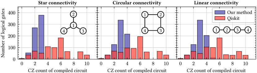
Figure 1: Distributions of $CZ$ counts over the logical Clifford group $\mathcal{C}^{2}/\mathcal{P}^{2}$ of the $\llbracket 4,2,2\rrbracket$ iceberg code for the hardware-tailored circuit implementations from Tab. 1. The three hardware connectivities, to which the circuit implementations have been tailored, are shown as insets. For comparison, we also show distributions of $CZ$ counts obtained via a straightforward Qiskit-based approach. Our method achieves lower two-qubit gate counts by incorporating the gauge freedom from Theorem 2 into the optimization process.

V Use case examples

In this section, we apply our framework from Sec. III in order to construct hardware-tailored circuit implementations for concrete logical Clifford gates and stabilizer codes. The selected use cases serve as proof-of-principle demonstrations, highlighting different strengths of our new techniques. First, in Sec. V.1 we construct the full logical Clifford group for the $\llbracket 4,2,2\rrbracket$ iceberg code under various connectivity constraints. This illustrates the flexibility of our method and demonstrates that the selected circuit implementations are not cherry-picked. In Sec. V.2, we present a logical $CX$ gate for the $\llbracket 12,2,3\rrbracket$ twisted toric code. This shows that our methods scale to experimentally relevant system sizes and effectively tackles the so-called addressability problem: how can one implement logical gates for QECCs whose logical qubits are delocalized across all physical qubits? In Sec. V.3, we construct logical Hadamard gates for the $\llbracket 8,3,2\rrbracket$ color code and make them fault-tolerant (FT) by carefully applying Lemma 4 from Sec. IV. This demonstrates that our circuit implementations can indeed be made FT through a second construction step, and simultaneously represents a significant circuit engineering milestone for early-FT experiments with the $\llbracket 8,3,2\rrbracket$ code, where highly-efficient FT logical Hadamard gate implementations were previously lacking.

V.1 $\llbracket 4,2,2\rrbracket$ iceberg code

Connectivity	$CZ$ count		Runtime
	max	avg.	max	avg.
Star	6	2.5	$3600\mskip 3.0mu\mathrm{s}$	$61\mskip 3.0mu\mathrm{s}$
Circular	4	3.0	$\phantom{1}436\mskip 3.0mu\mathrm{s}$	$85\mskip 3.0mu\mathrm{s}$
Linear	5	3.0	$\phantom{1}508\mskip 3.0mu\mathrm{s}$	$29\mskip 3.0mu\mathrm{s}$

Table 1: Circuit cost ($CZ$ count) and classical preprocessing cost (runtime) for constructing hardware-tailored circuit implementations in the worst case (max) and on average (avg.) for all 720 logical Clifford gates of the $\llbracket 4,2,2\rrbracket$ iceberg code for three different connectivities, see Fig. 1. Our circuit implementations are constructed by solving the IQCP in Eq. 23 using our Gurobi-based open-source software, applied to an ansatz circuit $A_{l}$ of length $l=3$ with a timeout of $3600\mskip 3.0mu\mathrm{s}$. All computations were carried out on four cores of an Intel Xeon CPU E5-2695 v2 @$2.40\mskip 3.0mu\mathrm{GHz}$ with $20\mskip 3.0mu\mathrm{GB}$ of RAM. The solver performs reliably and fast.

The first QECC for which we construct hardware-tailored logical Clifford gates is the four-qubit iceberg code Rains (1997). This $\llbracket 4,2,2\rrbracket$ code belongs to a family of $\llbracket n,n-2,2\rrbracket$ codes with stabilizer generators $X^{\otimes n}$ and $Z^{\otimes n}$, where $n$ is even. The $\llbracket 4,2,2\rrbracket$ iceberg code has $k=2$ logical qubits and therefore $|\mathcal{C}^{2}/\mathcal{P}^{2}|=720$ logical Clifford gates. Each of them is implementable in $12,288$ different gauges, recall Theorem 2. Leveraging our new techniques, we optimize over all gauges and a variety of circuit templates (ansätze) to identify circuit implementations that minimize the number of $CZ$ gates. To demonstrate the flexibility of our method, we consider three connectivities: star, circular, and linear, as shown in the insets of Fig. 1. For all three connectivities and every logical Clifford gate, we succeed in constructing a circuit implementation with no more than three CZLs and four SCLs, i.e., with an ansatz $U_{A_{l}}$ of length $l=3$. In Tab. 1, we present the maximum and average two-qubit gate counts of the constructed circuits, along with the maximum and average runtime of the solver that found them. In all cases, we see that no more than six physical $CZ$ gates are required for implementing a logical two-qubit Clifford circuit. We observe no significant difference in the quality of the obtained circuits.

Regarding the runtime of our classical circuit constructor, it is important to note that the leveraged Gurobi solver operates in two phases. First, it identifies a feasible solution to Eq. 23, corresponding to a valid circuit implementation of the target logical gate. Then, it attempts to prove optimality by searching for better feasible points and, if successful, replaces the initial solution with an improved one. Since we aim to construct $3\times 720$ circuit implementations, we impose a one-hour timeout on the Gurobi solver. As shown in Tab. 1, this timeout is only reached in the case of star connectivity. Even then, it affects only the proof of optimality; the solver still produced valid and high-quality solutions for all 720 logical Clifford gates.

We also compare our circuit implementations to readily obtainable baseline alternatives. For every logical Clifford gate, we use a Qiskit optimizer Qiskit contributors (2023) to compress the trivial implementation $U_{\text{triv}}$ defined in Sec. III.2. Since Qiskit does not support optimization over gauges $F\in\mathcal{F}$, we fix $F=\mathbbm{1}$ prior to optimization. We do not attempt a brute-force search over all $12,288$ possible gauges. After obtaining a circuit, we transpile it to the three hardware connectivities under consideration. For each connectivity, we present two histograms in Fig. 1, showing the two-qubit gate counts for our method (blue) and the Qiskit baseline (red). Our circuits consistently achieve lower $CZ$ counts compared to the Qiskit alternatives. Furthermore, our circuits exhibit virtually no outliers (apart from twelve instances with six $CZ$ gates), further underscoring the advantage of a global optimization approach over conventional circuit optimization techniques.

V.2 $\llbracket 12,2,3\rrbracket$ twisted toric code

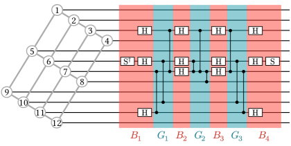
Figure 2: A hardware-tailored circuit implementation of the $\overline{CX_{2,1}}$ gate for the $\llbracket 12,2,3\rrbracket$ twisted toric code. The circuit (right) is tailored to a square-grid connectivity (left) and requires nine $CZ$ gates. It was constructed by solving Eq. 23 using an ansatz $U_{A_{l}}$ with $l=3$ controlled-$Z$ gate layers (CZLs) and four single-qubit Clifford gate layers (SCLs). The evident symmetry suggests that computer-generated circuits like this might be generalizable to larger twisted toric codes.

Next, we consider the $\llbracket 12,2,3\rrbracket$ twisted toric code Breuckmann and Eberhardt (2021b) and tackle the aforementioned addressability problem. When constructing hardware-tailored logical circuit implementations for this code, we do not explicitly exploit any of its symmetries. Instead, we simply inform our solver for Eq. 23 that the stabilizer group is generated by $X_{1}X_{2}X_{6}X_{7}$, $X_{1}X_{4}X_{11}X_{12}$, $X_{2}X_{3}X_{9}X_{10}$, $X_{3}X_{4}X_{5}X_{8}$, $X_{5}X_{6}X_{10}X_{11}$, $Z_{1}Z_{2}Z_{9}Z_{12}$, $Z_{1}Z_{4}Z_{5}Z_{6}$, $Z_{2}Z_{3}Z_{7}Z_{8}$, $Z_{3}Z_{4}Z_{10}Z_{11}$, and $Z_{5}Z_{8}Z_{9}Z_{10}$, and that the logical Pauli operators are chosen as $\overline{X}_{1}=X_{1}X_{5}X_{9}$, $\overline{Z}_{1}=Z_{1}Z_{2}Z_{3}Z_{4}$, $\overline{X}_{2}=X_{1}X_{2}X_{3}X_{4}$, and $\overline{Z}_{2}=Z_{2}Z_{6}Z_{10}$. From Eq. 15, we know that for each logical Clifford gate, there exist approximately $1.5\times 10^{58}$ different implementations that differ only in their action on states outside the code space.

Assuming a $3\times 4$ square-grid connectivity, we tailor circuit implementations of the logical controlled-$X$ gate with control qubit 2 and target qubit 1. Note that our method is not limited to this example. First, we consider an ansatz length $l=2$ and succeed in constructing a circuit with eleven $CZ$ gates (not shown). By increasing to $l=3$, we find an even shorter circuit with only nine $CZ$ gates that is displayed in Fig. 2. Interestingly, this computer-generated circuit appears to exhibit a nontrivial structure: the first and the last SLCs are inverses of each other, i.e., $B_{1}=B_{4}^{-1}$. The same is true for the (self-inverse) inner SCLs and the outer CZLs, i.e., $B_{2}=B_{3}^{-1}=B_{3}$ and $G_{1}=G_{3}^{-1}=G_{3}$. This emergent structure spurs hope that, despite the NP-hardness of solving Eq. 23, our software can be used to construct and analyze small-scale logical gates, and that these constructions, once understood, may be analytically generalized to larger codes. In this context, it is important that one can efficiently verify whether a candidate circuit implements a desired logical Clifford gate, see Lemma 7 in App. A.

V.3 $\llbracket 8,3,2\rrbracket$ color code

Gate	Teleportation-based Wang et al. (2024)	Hardware-tailored
$\overline{{H}}$	CZ count: 26 Consumed qubits: 10	CZ count: 13 Consumed. qubits: 1
$\overline{{H}^{\otimes 2}}$	CZ count: 37 Consumed qubits: 13	CZ count: 16 Consumed qubits: 1
$\overline{{H}^{\otimes 3}}$	CZ count: 63 Consumed qubits: 23	CZ count: 19 Consumed qubits: 1

Table 2: Resource requirements of circuit implementations of FT logical Hadamard gates for the $\llbracket 8,3,2\rrbracket$ color code. Consumed qubits refers to the number of state initializations and measurements required for a single implementation of the logical gate. The method from Ref. Wang et al. (2024) relies on a teleportation routine into the $\llbracket 4,2,2\rrbracket$ iceberg code. In contrast, our hardware-tailored circuit implementations require only a single auxiliary qubit to achieve fault tolerance, see Fig. 3.

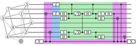
(a) Logical Hadamard gate, $\overline{{H}_{1}}$, on the first logical qubit.

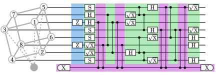
(b) Logical Hadamard gates, $\overline{H^{\otimes 2}_{1,2}}$, on two logical qubits.

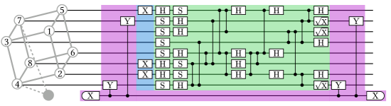
(c) Logical Hadamard gates, $\overline{H^{\otimes 3}_{1,2,3}}$, on all three logical qubits.

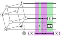
(d) Logical phase gate, $\overline{{S}_{1}}$, on the first logical qubit.

Figure 3: Hardware-tailored circuit implementation of FT logical (a-c) Hadamard and (d) phase gates for the $\llbracket 8,3,2\rrbracket$ color code. By rotating the cube, other logical qubits can be addressed. The unitary Clifford subcircuits (green) are tailored to a cube connectivity (left) by solving the IQCP in Eq. 23. Then, the Pauli frame (blue) is adjusted by applying Theorem 2 in Ref. Dehaene and De Moor (2003). Finally, a suitable flag gadget (purple) is constructed by applying Lemma 4 to make the circuit implementation fault-tolerant, where dashed lines in the graph on the left indicate the connectivity required by the flag gadget. Using stim Gidney (2021), we verify that every fault (recall Sec. IV) results in a detectable error. For the Hadamard gates, fault tolerance is independently confirmed through circuit-level noise simulations, see Fig. 4.

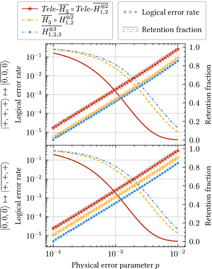
Figure 4: Logical error rate (left $y$-axis) and retained fraction (right $y$-axis) of shots after discarding executions with non-trivial syndromes, based on circuit-level simulations of the gates from Tab. 2. The parameter $p$ ($x$-axis) and details of the simulated circuits are explained in App. D. Each data point represents an average over $10^{8}$ circuit executions simulated using stim Gidney (2021). All protocols are fault-tolerant, and the teleportation-free approaches perform better due to their lower resource demands, see Tab. 2.

The final code considered in this paper is the $\llbracket 8,3,2\rrbracket$ color code, often referred to as the “smallest interesting color code” due to its remarkable ability of supporting a transversal non-Clifford gate Campbell (2016). More precisely, applying the operator $(T\otimes T^{\dagger})^{\otimes 4}$ implements the gate $CCZ=\mathrm{diag}(1,\ldots,1,-1)$ on the three logical qubits. It is well known that the gate set comprising $CCZ$ and Hadamard gates is universal in a certain sense Shi (2003), however, it is also worth noting that the group they generate contains only real matrices. As such, there is value in augmenting the gate set with the Clifford gate $S=\mathrm{diag}(1,\mathrm{i}\mkern 1.0mu)$. Since the $CCZ$ gate is already transversal, the Eastin–Knill theorem implies that the logical Hadamard gate for the $\llbracket 8,3,2\rrbracket$ code must require a more complex circuit implementation Eastin and Knill (2009).

To our knowledge, the only fully worked-out example of implementing FT logical Hadamard gates is based on a teleportation approach Wang et al. (2024). In this protocol, one or two logical qubits are teleported into the $\llbracket 4,2,2\rrbracket$ iceberg code, which supports a Swap-transversal two-qubit Hadamard gate. After the operation is applied, the qubits are teleported back into the color code. We refer to these protocols as $\smash{\textit{Tele-}\overline{H}}$ and $\smash{\textit{Tele-}\overline{H^{\otimes 2}}}$ and provide their resource costs in Tab. 2. For example, the $\textit{Tele-}\overline{H}$ protocol has a $CZ$ count of 26 and consumes a total of ten auxiliary qubits (four for the iceberg code and six for flagging). Similarly, one can implement Hadamard gates on all three logical qubits of the $\llbracket 8,3,2\rrbracket$ color code by applying first $\smash{\textit{Tele-}\overline{H^{\otimes 2}_{1,2}}}$ then $\smash{\textit{Tele-}\overline{H_{3}}}$, with costs ($CZ$ count and consumed qubits) that simply add up. If resets are available and parallelization is sacrificed, only six auxiliary qubits are required at the same time. Notably, no experimental implementation of teleportation-based Hadamard gates for the $\llbracket 8,3,2\rrbracket$ code has been reported in the existing literature.

With the methods developed in this paper, we are able to directly decompose logical Clifford circuits into physical ones, without relying on teleportation into a second code that supports these gates transversally. In Fig. 3, we present such teleportation-free implementations of single- and multi-qubit logical Hadamard gates on an arbitrary number of logical qubits alongside a single-qubit logical phase gate. Moreover, we present flag gadgets that make these circuits FT in the sense defined in Sec. IV. In all cases, a single flag qubit suffices to catch all undetectable errors that would be introduced by the hardware-tailored circuits alone. In other words, the second flag qubit in the construction of Lemma 4 is not required in this context due to the absence of undetectable hook errors. For the two-qubit logical Hadamard gate shown in Fig. 3(b), we need to apply Lemma 4 twice. However, note that it is possible to reuse a single flag qubit without resetting it. The total resource requirements of our teleportation-free circuits can be directly inferred from Fig. 3 and are provided in Tab. 2 for a direct comparison with the teleportation-based Hadamard gates from Ref. Wang et al. (2024). Our circuits consume an order of magnitude fewer qubits and require only half as many physical $CZ$ gates for the single- and two-qubit logical Hadamard gates. To realize a three-qubit logical Hadamard gate using the teleportation-based approach, two circuits must be applied sequentially, resulting in additive resource costs. This sequential approach can be avoided with the flexible method developed in Sec. III, resulting in a three times cheaper (in terms of $CZ$ count) implementation of the three-qubit logical Hadamard gate.

To predict the performance of our circuit implementations, we carry out circuit-level simulations using stim Gidney (2021). Our simulations are based on the error model described in App. D, where all physical error rates are proportional to a single parameter $p$. We compare the following three methods for FT mapping $\smash{\ket{\overline{0,0,0}}}$ to $\smash{\ket{\overline{\mathord{+},\mathord{+},\mathord{+}}}}$, and vice versa, and present the simulation results in Fig. 4. First, we apply the sequence of two teleportation-based circuits from Ref. Wang et al. (2024) to implement $\smash{\textit{Tele-}\overline{H_{3}}}\circ\smash{\textit{Tele-}\overline{H^{\otimes 2}_{1,2}}}$ (red stars). Second, $\smash{\overline{H_{3}}\circ\overline{H^{\otimes 2}_{1,2}}}$ is implemented by sequentially applying the circuits from Fig. 3(b) and a straightforward adaptation of Fig. 3(a) (yellow plusses). Finally, we also apply $\smash{\overline{H^{\otimes 3}_{1,2,3}}}$ in a single step, using the circuit from Fig. 3(c) (blue circles). For details about FT state preparation and readout, see App. D. In all cases, we observe in Fig. 4 the characteristic FT scaling of the logical error rate to be $O(p^{2})$. This confirms that every single fault in the circuit is detected and removed in a postprocessing step. The fraction of shots retained after discarding all circuit executions with violated detectors is plotted as a continuous curve in the background of Fig. 4. For both hardware-tailored options, we observe that this retained fraction decreases from nearly 100% at $p=10^{-4}$ to about $10\%$ at $p=10^{-2}$. The teleportation-based approach exhibits the same qualitative behavior, but with a significantly lower retained fraction throughout. Regarding the logical error rates, we observe that the hardware-tailored circuit performing all logical Hadamard gates simultaneously (blue circles) yields the best performance. This is expected, as it requires the fewest resources and thus introduces the fewest potential error mechanisms, recall Tab. 2. Strikingly, this represents an improvement of approximately one order of magnitude over the teleportation-based protocol. A minor effect visible in Fig. 4 is that the error rates are slightly larger for the protocol mapping $\ket{\overline{0,0,0}}$ to $\ket{\overline{\mathord{+},\mathord{+},\mathord{+}}}$ (lower panel) than for the reverse direction (upper panel). This suggests the presence of more detrimental error mechanisms when the three-fold Hadamard gate is applied to $\ket{\overline{\mathord{+},\mathord{+},\mathord{+}}}$.

VI Conclusion

In this work, we developed powerful techniques to decompose logical Clifford circuits into physical ones for arbitrary stabilizer codes. Starting from the symplectic representation of the Clifford group, we introduced a class of hardware-tailored ansatz circuits parameterized by binary variables. Similarly, we parameterized all possible gauges of a target logical gate by identifying the group of logical Clifford stabilizers associated with the given code. This framework ultimately reduces circuit construction to solving and optimizing an integer quadratically constrained program (IQCP). We provide an open-source implementation, available as a Python package on https://github.com/erkue/htlogicalgates.

We have demonstrated the viability of our approach across a variety of gates and quantum error-correcting codes. To support future experiments in early fault tolerance, we tailored logical Hadamard gates with flag gadgets for the $\llbracket 8,3,2\rrbracket$ color code. Through circuit-level noise simulations, we have shown that our constructions not only consume significantly fewer auxiliary qubits than an existing teleportation-based approach but also reduce the logical error rate by an order of magnitude.

From a broader perspective, the approach introduced here builds upon and extends ideas from global optimization Miller et al. (2024) to identify highly efficient, hardware-tailored circuits for the implementation of quantum error-correcting codes. It complements circuit design methodologies based on algebraic rewrites—such as those using the ZX calculus Coecke and Duncan (2011) or three-colored formalisms Magdalena de la Fuente et al. (2025)—which sequentially manipulate and optimize circuits through structured transformations.

Our framework does not rely on underlying symmetries of the codes or their logical gates. As a result, it provides a flexible starting point for in-depth analyses of stabilizer codes and their logical Clifford gates under realistic hardware constraints. In future work, our approach may be adapted to address related problems in circuit discovery. For instance, by adapting the IQCP presented in this paper, it may be possible to construct hardware-tailored state preparation circuits, addressing the well-studied problem of fault-tolerant logical state preparation Zen et al. (2024); Peham et al. (2025). Moreover, our framework could potentially be extended to design hardware-tailored circuits for code switching Anderson et al. (2014); Bombín (2015); Butt et al. (2024).

VII Acknowledgments

The authors would like to thank Antonio Anna Mele, Lennart Bittel, David Pahl, Lukas Pahl, Arthur Pesah, and Armanda Quintavalle for stimulating discussions. This project has received financial support by the Unitary Foundation, the BMBF (QSolid, MuniQC-Atoms, QuSol), the Munich Quantum Valley, Berlin Quantum, the Quantum Flagship programs MILLENION and PASQUANS2, the DFG (CRC 183), the European Research Council (DebuQC), and the Alexander-von-Humboldt Foundation. This research has been sponsored by IARPA and the Army Research Office, under the Entangled Logical Qubits program, and was accomplished under Cooperative Agreement Number W911NF-23-2-0212. The views and conclusions contained in this document are those of the authors and should not be interpreted as representing the official policies, either expressed or implied, of IARPA, the Army Research Office, or the U.S. Government. The U.S. Government is authorized to reproduce and distribute reprints for Government purposes notwithstanding any copyright notation herein. J.R. is funded by by EPSRC Grants EP/T001062/1 and EP/X026167/1.

Appendix A Characterization of logical Clifford gates

In this appendix, we review several well-known results on logical gates, with an emphasis on Clifford operations for stabilizer codes. This provides the necessary background to understand the origin of their gauge freedom, which will be fully characterized in Theorem 2 and further simplified in Corollary 3. Throughout this section, let $\mathcal{L}$ be the code space of an $\llbracket n,k,d\rrbracket$ stabilizer code, $\{S_{1},\ldots,S_{n-k}\}$ a set of stabilizer generators, and $\mathcal{S}=\langle S_{1},\ldots,S_{n-k}\rangle$ its stabilizer group. Moreover, let $\smash{\overline{X_{1}},\ldots,\overline{X_{k}}}$ and $\smash{\overline{Z_{1}},\ldots,\overline{Z_{k}}}$ denote a choice of logical Pauli-$X$ and -$Z$ operators for $\mathcal{L}$, respectively.

Let us start with the following lemma, which will only be used in this appendix.

Lemma 5 (Inverses of logical gates are also logical gates).

Let $U\in\mathcal{U}(2^{n})$ be an $n$-qubit unitary. Then, $U$ is a logical gate for $\mathcal{L}$ if and only if (iff) the same is true for $U^{\dagger}$.

Proof.

It suffices to prove that the condition is sufficient as the roles of $U$ and $U^{\dagger}$ are interchangeable. Thus, let $U$ be a logical gate, i.e., for all code words $\smash{\ket{{\psi}}}\in\mathcal{L}$ it holds $U\smash{\ket{{\psi}}}\in\mathcal{L}$. Let $\mathcal{B}=\smash{\{\ket{{\psi_{1}}},\ldots,\ket{{\psi_{2^{k}}}}\}}$ be a vector space basis of $\mathcal{L}$. Then, $U\mathcal{B}=\smash{\{U\ket{{\psi_{1}}},\ldots,U\ket{{\psi_{2^{k}}}}}\}$ is a subset of $\mathcal{L}$. Since $U$ is injective, $U\mathcal{B}$ is linearly independent. Because of $|U\mathcal{B}|=2^{k}$, it follows that $\mathcal{B}^{\prime}=U\mathcal{B}$ is a basis of $\mathcal{L}$. By construction, the inverse of $U$ maps $\mathcal{B}^{\prime}$ to $U^{\dagger}\mathcal{B}^{\prime}=\mathcal{B}\subset L$. By linearity, it follows that $U^{\dagger}\ket{{\psi}}$ lies in $\mathcal{L}$ for all $\ket{{\psi}}\in\mathcal{L}$, which finishes the proof. ∎

Next, we formulate a useful condition for verifying that a Clifford circuit implements a gate on the logical level.

Lemma 6 (Logical Cliffords permute the stabilizer group).

Let $U\in\mathcal{C}^{n}$ be an $n$-qubit Clifford gate. Then, the following conditions are equivalent:

• $U$ is a logical gate for $\mathcal{L}$.

• $U$ is a logical Clifford gate for $\mathcal{L}$.

• For all $S\in\mathcal{S}$, we have $USU^{\dagger}\in\mathcal{S}$.

• For all $S\in\{S_{1},\ldots,S_{n-k}\}$, we have $USU^{\dagger}\in\mathcal{S}$.

Proof.

The implications “(i)$\,\Rightarrow$(ii)” and “(iii)$\,\Rightarrow$(iv)” are trivial. The reverse implications follow from the fact that $UPU^{\dagger}$ is a Pauli operator whenever $P$ is, and from a standard argument that expands an arbitrary stabilizer operator $S\in\mathcal{S}$ into a product of stabilizer generators. Let us now prove the remaining implications.
(i)$\,\Rightarrow$(iii): Let $S\in\mathcal{S}$. Since $U$ is a Clifford gate, $USU^{\dagger}$ is a Pauli operator. Let us show that $USU^{\dagger}$ stabilizes the code space. Thus, let $\ket{\smash{\psi}}\in\mathcal{L}$ be an arbitrary code word. From Lemma 5, we know that $U^{\dagger}$ is a logical operator. Hence, we have $U^{\dagger}\smash{\ket{{\psi}}}\in\mathcal{L}$ and, therefore, $SU^{\dagger}\smash{\ket{{\psi}}}=U^{\dagger}\smash{\ket{{\psi}}}$. This, in turn, implies $USU^{\dagger}\smash{\ket{{\psi}}}=UU^{\dagger}{\ket{{\psi}}}=\ket{\smash{\psi}}$. In other words, $USU^{\dagger}$ is a stabilizer operator.
(iii)$\,\Rightarrow$(i): Let $\ket{\smash{\psi}}\in\mathcal{L}$. We have to show $U\ket{\smash{\psi}}\in\mathcal{L}$. By assumption, we have $US=SU$ for all $S\in\mathcal{S}$. This implies $U\ket{\smash{\psi}}=US\ket{\psi}=SU\ket{\psi}$. In other words, the state vector $U\ket{\psi}$ lies in the $+1$-eigenspace of all operators $S\in\mathcal{S}$, i.e., in the code space $\mathcal{L}$. This finishes the proof. ∎

Finally, we apply Schur’s lemma William Fulton (2013) to prove that Clifford gates act the same on the logical level iff they transform the logical Pauli operators identically, up to stabilizers.

Lemma 7 (Equivalence of different logical Clifford gates).

Let $U,V\in\mathcal{C}^{n}$ be two logical Clifford gates for $\mathcal{L}$. The following conditions are equivalent:

• There is a global phase $\alpha\in\mathbbm{R}$ such that for all $\ket{\psi}\in\mathcal{L}$ it holds $U\ket{\psi}=e^{\mathrm{i}\mkern 1.0mu\alpha}V\ket{\psi}$.

• For every logical qubit $i\in\{1,\ldots,k\}$, there exist stabilizer operators $S,S^{\prime}\in\mathcal{S}$ with $U\overline{X_{i}}U^{\dagger}=V\overline{X_{i}}V^{\dagger}S$ and $U\overline{Z_{i}}U^{\dagger}=V\overline{Z_{i}}V^{\dagger}S^{\prime}$.

Proof.

(i)$\,\Rightarrow$(ii): It suffices to show that $P=U\overline{X_{i}}U^{\dagger}V\overline{X_{i}}V^{\dagger}$ is a stabilizer operator; the case of $\overline{Z_{i}}$ can be treated the same. Thus, let $\ket{\psi}\in\mathcal{L}$ be an arbitrary code word. By assumption, we have $P\ket{\psi}=(e^{\mathrm{i}\mkern 1.0mu\alpha}V)X_{i}(e^{\mathrm{i}\mkern 1.0mu\alpha}V)^{\dagger}V\overline{X_{i}}V^{\dagger}\ket{\psi}$ because this calculation takes place in $\mathcal{L}$ entirely. Therefore, $P\ket{\psi}=\ket{\psi}$, which implies $P\in\mathcal{S}$, as claimed.
(ii)$\,\Rightarrow$(i): We want to apply Schur’s lemma to show that the linear map $f:\mathcal{L}\rightarrow\mathcal{L},\ket{\psi}\mapsto V^{\dagger}U\ket{\psi}$ is proportional to $\text{id}_{\mathcal{L}}$. Then, the proportionality constant must be of the form $e^{\mathrm{i}\mkern 1.0mu\alpha}$ because $f$ is unitary. For this, we point out that the representation $g:G=\langle\overline{X_{i}},\overline{Z_{i}}\ |\ i\in\{1,\ldots,k\}\rangle\rightarrow\text{GL}(\mathcal{L})$ that sends an $n$-qubit Pauli operator to itself is irreducible. We need to show that $f$ and $g$ commute. Thus, let $P\in G$ and $\ket{\psi}\in\mathcal{L}$ be arbitrary. By assumption, there is some $S\in\mathcal{S}$ with $UPU^{\dagger}=VPV^{\dagger}S$. This yields $f(g(P)\ket{\psi})=V^{\dagger}UP\ket{\psi}=V^{\dagger}(UPU^{\dagger})U\ket{\psi}=V^{\dagger}(VPV^{\dagger}S)U\ket{\psi}=PV^{\dagger}U\ket{\psi}=g(P)f(\ket{\psi})$. Therefore, Schur’s lemma applies, which finishes the proof. ∎

Appendix B Proof of Theorem 2

In this appendix, we prove Theorem 2. More precisely, we show that

$$\mathcal{F}=\{F\in\operatorname{Sp}(\mathbbm{F}_{2}^{2n})\ |\ F\text{ obeys \lx@cref{creftype~refnum}{eq:freedom_matrix}}\}$$ (24)

serves as the gauge group for logical Clifford operations whose action is specified only on the logical subspace and may differ outside the code space. Moreover, we prove that the cardinality of $\mathcal{F}$ is given by the expression in Eq. 15.

Proof.

Our first claim is that $\mathcal{F}$ is a group. To show this, we write the elements $F\in\mathcal{F}$ in block form as in

$$F=\begin{bmatrix}F^{xx}&0_{n}\\ F^{zx}&F^{zz}\end{bmatrix},$$ (25)

where $0_{n}\in\mathbbm{F}_{2}^{n\times n}$ denotes the all-zero matrix. The constraints from Eq. 14 on the blocks are given by

$$F^{xx}=\begin{bmatrix}\mathbbm{1}_{k}&\ast&\cdots&\ast\\ 0&\ast&\cdots&\ast\\ \vdots&\vdots&\ddots&\vdots\\ 0&\ast&\cdots&\ast\\ \end{bmatrix},\hskip 14.22636ptF^{zz} =\begin{bmatrix}\mathbbm{1}_{k}&0&\cdots&0\\ \ast&\ast&\cdots&\ast\\ \vdots&\vdots&\ddots&\vdots\\ \ast&\ast&\cdots&\ast\\ \end{bmatrix},$$ (26)

$$\text{and }\hskip 5.69054ptF^{zx} =\begin{bmatrix}0_{k}&\ast&\cdots&\ast\\ \ast&\ast&\cdots&\ast\\ \vdots&\vdots&\ddots&\vdots\\ \ast&\ast&\cdots&\ast\\ \end{bmatrix}.$$ (27)

Clearly, $F=\mathbbm{1}_{2n}$ fulfills these constraints, proving $\mathbbm{1}_{2n}\in\mathcal{F}$. Taking the product of two matrices $F,\tilde{F}\in\mathcal{F}$ results in

$$F\tilde{F}=\begin{bmatrix}F^{xx}\tilde{F}^{xx}&0_{n}\\ F^{zx}\tilde{F}^{xx}+F^{zz}\tilde{F}^{zx}&F^{zz}\tilde{F}^{zz}\end{bmatrix}.$$ (28)

It is straightforward to verify that $F^{xx}\tilde{F}^{xx}$ and $F^{zz}\tilde{F}^{zz}$ inherit the constraints of Eq. 26. Similarly, both $F^{zx}\tilde{F}^{xx}$ and $F^{zz}\tilde{F}^{zx}$ obey the constraints of Eq. 27, which proves $F\tilde{F}\in\mathcal{F}$. This shows that $\mathcal{F}$ is closed under taking products. Hence, it is also closed under taking inverses because $\mathcal{F}\subset\mathbbm{F}_{2}^{2n\times 2n}$ is clearly finite. This proves that $\mathcal{F}$ is a group.

As mentioned in the main text, $\mathcal{F}$ can be understood as the subgroup of non-Pauli Clifford stabilizers of the code space $\mathcal{L}$ of an $\llbracket n,k,d\rrbracket$ code. Next we will show that $\mathcal{F}$ is in bijection to the different choices of physical Clifford operators (modulo Paulis) that implement a given logical Clifford gates. In that sense, the elements of $\mathcal{F}$ correspond to different gauges of logical Clifford operators. To distinguish it from the concept of gauge groups in subsystem QECCs Lidar and Brun (2013); Vuillot et al. (2019); Li et al. (2019), we refer to $\mathcal{F}$ as the freedom gauge group throughout this paper.

We need to show that $U_{EC^{\prime}FE^{-1}}$ implements $U_{C}\in\mathcal{C}^{k}$ on the logical level whenever $F\in\mathcal{F}$ and, conversely, that every $n$-qubit Clifford operation that does so is of the form $U_{EC^{\prime}FE^{-1}}$ for some $F\in\mathcal{F}$. For both statements we will make use of the fact that the encoding circuit $U_{E}$ maps Pauli-$Z$ operators on qubits $k+1$ to $n$ to stabilizers $S\in\langle S_{1},\ldots,S_{n-k}\rangle$ and arbitrary Pauli operators on qubits $1$ to $k$ to logical Pauli operators $\bar{P}\in\langle\bar{X}_{1},\bar{Z}_{1},\ldots,\bar{X}_{k},\bar{Z}_{k}\rangle$. To make this more precise, we introduce binary vectors $\mathbf{s}_{j},\mathbf{s}^{\prime}_{j},\mathbf{x}_{i},\mathbf{x}^{\prime}_{i},\mathbf{z}_{i},\mathbf{z}^{\prime}_{i}\in\mathbbm{F}_{2}^{n}$ such that $S_{j-k}\propto X^{\mathbf{s}_{j}}Z^{\mathbf{s}^{\prime}_{j}}$, for all $j\in\{k+1,\ldots,n\}$ and $\bar{X}_{i}\propto X^{\mathbf{x}_{i}}Z^{\mathbf{x}^{\prime}_{i}}$, $\bar{Z}_{i}\propto X^{\mathbf{z}_{i}}Z^{\mathbf{z}^{\prime}_{i}}$ for all $i\in\{1,\ldots,k\}$, see Eq. 9. Then, we have

$$E\begin{bmatrix}\mathbf{e}_{i}\\ 0\end{bmatrix}=\begin{bmatrix}\mathbf{x}_{i}\\ \mathbf{x}^{\prime}_{i}\end{bmatrix},\hskip 5.69054ptE\begin{bmatrix}0\\ \mathbf{e}_{i}\end{bmatrix} =\begin{bmatrix}\mathbf{z}_{i}\\ \mathbf{z}^{\prime}_{i}\end{bmatrix},$$ (29)

$$\hskip 5.69054pt\text{and}\hskip 5.69054ptE\begin{bmatrix}0\\ \mathbf{e}_{j}\end{bmatrix} =\begin{bmatrix}\mathbf{s}_{j}\\ \mathbf{s}^{\prime}_{j}\end{bmatrix},$$ (30)

where $\mathbf{e}_{l}=(\delta_{l,l^{\prime}})_{l^{\prime}=1}^{n}\in\mathbbm{F}_{2}^{n}$ denotes a standard basis vector.

First, assume we have a Clifford operation $U_{M}\in\mathcal{C}^{n}$ that is represented by $M=EC^{\prime}FE^{-1}$ for some $F\in\mathcal{F}$. We have to show that $U_{M}$ acts as $C$ on the logical level. For every $j\in\{1,\ldots,n-k\}$, we find that $U_{M}S_{j}U_{M}^{\dagger}$ is represented by

$$M\begin{bmatrix}\mathbf{s}_{j}\\ \mathbf{s}^{\prime}_{j}\end{bmatrix}= E\sum_{l=k+1}^{2n}F_{l+n,j+n}\begin{bmatrix}0\\ \mathbf{e}_{l}\end{bmatrix},$$ (31)

where we have used Eq. 30 and the fact that $F^{xz}=0$, which holds by definition of $F\in\mathcal{F}$. Again applying Eq. 30, we further find

$$M\begin{bmatrix}\mathbf{s}_{j}\\ \mathbf{s}^{\prime}_{j}\end{bmatrix}= \sum_{l=k+1}^{2n}F_{l+n,j+n}\begin{bmatrix}\mathbf{s}_{l}\\ \mathbf{s}^{\prime}_{l},\end{bmatrix}$$ (32)

which implies $U_{M}S_{j}U_{M}^{\dagger}\in\mathcal{S}$. Therefore, Lemma 6 applies, and shows that $U_{M}$ is a logical operator. To determine its logical action, let us first compute the vectors that represents $U_{M}\overline{X_{i}}U_{M}^{\dagger}$ for all $i\in\{1,\ldots,k\}$, that is

$$M\begin{bmatrix}\mathbf{x}_{i}\\ \mathbf{x}^{\prime}_{i}\end{bmatrix} =EC^{\prime}\begin{bmatrix}\mathbf{e}_{i}\\ 0\end{bmatrix}+\sum_{l=k+1}^{2n}F_{l+n,i}\begin{bmatrix}\mathbf{s}_{l}\\ \mathbf{s}^{\prime}_{l}\end{bmatrix}.$$ (33)

The first term in Eq. 33 represents the logical Pauli operator to which the $i$-th Pauli-$X$ operator is transformed into, while the second term reflects that this mapping is defined modulo stabilizers. Similarly, we find

$$U_{M}\overline{Z_{i}}U_{M}^{\dagger}=\overline{U_{C}Z_{i}U_{C}^{\dagger}}S^{\prime}_{i}$$ (34)

for some $S^{\prime}_{i}\in\mathcal{S}$. Therefore, Lemma 7 applies, and we have shown that $U_{M}$ acts as $U_{C}\in\mathcal{C}^{k}$ on the logical level.

Next, we show the converse that every Clifford operation $U_{M}\in\mathcal{C}^{n}$ that implements $U_{C}\in\mathcal{C}^{k}$ on the logical level can be written as $M={EC^{\prime}FE^{-1}}$ for some freedom matrix $F\in\mathcal{F}$. Our strategy is to translate the constraints on $M$ imposed by Lemmata 6 and 7 into the constraints on $F$ that are shown in Eq. 14. To this end, we define the freedom matrix $F=C^{\prime-1}E^{-1}ME$. To prove $F\in\mathcal{F}$, we first apply $F$ to the unit vector corresponding to the unencoded $i$-th logical Pauli-$X$ operator from Eq. 29. By Eq. 29, this yields

$$F\begin{bmatrix}\mathbf{e}_{i}\\ 0\end{bmatrix} =C^{\prime-1}E^{-1}M\begin{bmatrix}\mathbf{x}_{i}\\ \mathbf{x}^{\prime}_{i}\end{bmatrix}$$ (35)

Next, we apply Lemma 7 to arrive at

$$F\begin{bmatrix}\mathbf{e}_{i}\\ 0\end{bmatrix} =\begin{bmatrix}\mathbf{e}_{i}\\ 0\end{bmatrix}+\sum_{l=k+1}^{n}f_{l+n,i}\begin{bmatrix}0\\ \mathbf{e}_{l}\end{bmatrix},$$

which proves the restrictions on $F$ shown in Eq. 14 for columns $1$ to $k$. Similarly, by repeating the calculation for the logical Pauli-$Z$ operators, we obtain the corresponding restrictions for columns $n+1$ to $n+k$. Finally, we analyze the constraints on $F$ that are imposed by how $U_{M}$ is allowed to transform stabilizer operators. By Lemma 6, we have

$$F\begin{bmatrix}0\\ \mathbf{e}_{j}\end{bmatrix} =C^{\prime-1}E^{-1}M\begin{bmatrix}\mathbf{s}_{j}\\ \mathbf{s}^{\prime}_{j}\end{bmatrix}$$ (37)

$$=\sum_{l=k+1}^{n}f_{l+n,j+n}\begin{bmatrix}0\\ \mathbf{e}_{l}\end{bmatrix},$$

which proves that also columns $n+k+1$ to $2n$ have to be of the form given in Eq. 14. Since there are no constraints, besides $F\in\operatorname{Sp}(\mathbbm{F}_{2}^{2n})$, on columns $k+1$ to $n$, this finishes the proof of $F\in\mathcal{F}$.

Finally, let us compute the order $|\mathcal{F}|$ of the freedom gauge group. Because every freedom matrix $F\in\mathcal{F}$ is invertible, the same must be true about the block matrix $F^{zz}$. By Eq. 26, this is the case iff the submatrix of size $(n-k)\times(n-k)$ in the bottom right of $F^{zz}$ is invertible. Besides this, there are no further constraints on the columns vectors of $F^{zz}$. Thus, there are

$$|\mathbbm{F}_{2}^{n-k}|^{k}\times|\operatorname{GL}(\mathbbm{F}_{2}^{n-k})|=2^{k(n-k)}\prod_{i=0}^{n-k-1}(2^{n-k}-2^{i})$$ (38)

possible choices for $F^{zz}$. Next, we write out the condition $F\in\operatorname{Sp}(\mathbbm{F}_{2}^{2n})$, i.e., $F^{T}\left[\begin{smallmatrix}0&\mathbbm{1}\\ \mathbbm{1}&0\end{smallmatrix}\right]F=\left[\begin{smallmatrix}0&\mathbbm{1}\\ \mathbbm{1}&0\end{smallmatrix}\right]$, which yields

$$(F^{xx})^{T}F^{zz} =\mathbbm{1}\text{ \ \ and}$$ (39)

$$\left((F^{xx})^{T}F^{zx}\right)^{T} =(F^{xx})^{T}F^{zx}.$$ (40)

By Eq. 39, the submatrix $F^{xx}=((F^{zz})^{T})^{-1}$ is uniquely determined through the choice of $F^{zz}$. Eq. 40 means that $(F^{xx})^{T}F^{zx}$ must be a symmetric matrix. Since we can regard $(F^{xx})^{T}$ as a bijective map, the number of allowed choices for $(F^{xx})^{T}F^{zx}$ and $F^{zx}$ are identical. There are in total $2^{n(n+1)/2}$ symmetric binary $n\times n$-matrices, however, not all of them are allowed by Eq. 14. Rows $1$ to $k$ of $F^{zz}$ and map columns $1$ to $k$ of $(F^{xx})^{T}F^{zx}$ to zero in $F^{zx}$, since $F^{zz}[(F^{xx})^{T}F^{zx}]=F^{zx}$. This reduces the number of free variables of $(F^{xx})^{T}F^{zx}$ by $k(k+1)/2$ for a given choice of $F^{zz}$ and $F^{xx}$. In total, this shows that the order of the freedom gauge group $\mathcal{F}$ is indeed given by the expression in Eq. 15, which finishes the proof of Theorem 2. ∎

This proof contains an explicit (albeit somewhat opaque) enumeration of all elements in the freedom gauge group $\mathcal{F}$. To better understand the role of $\mathcal{F}$, we rearrange Eq. 15 into

$$\begin{split}|\mathcal{F}|=&\underbrace{2^{2k(n-k)}}_{\text{(1)}}\underbrace{2^{(n-k)(n-k+1)/2}}_{\text{(2)}}\underbrace{\prod_{i=0}^{n-k-1}\left(2^{n-k}-2^{i}\right)}_{\text{(3)}}.\end{split}$$ (41)

Factor (3) in Eq. 41 is the number of ways in which the $n-k$ stabilizer generators can be mapped to a different choice of stabilizer generators. Similarly, factor (1) is the number of ways to correctly transform $2k$ logical Pauli operators modulo stabilizers, while factor (2) characterizes the additional freedom provided by the transformation of Pauli errors.

Appendix C Empirical runtimes of the IQCP solver

Code	Gate	Length $l$	$CZ$ count	Found	Optimality
$\llbracket 12,2,3\rrbracket$	$\overline{CX_{2,1}}$	$2$	$11$	$45\mskip 3.0mu\mathrm{min}$	$119\mskip 3.0mu\mathrm{min}$
		$3$	$9$	$76\mskip 3.0mu\mathrm{h}$	/
$\llbracket 8,3,2\rrbracket$	$\overline{H_{1}}$	$3$	$7$	$8\mskip 3.0mu\mathrm{min}$	$51\mskip 3.0mu\mathrm{min}$
		$4$	$7$	$21\mskip 3.0mu\mathrm{h}$	/
	$\overline{{H}^{\otimes 2}_{1,2}}$	$3$	8	$86\mskip 3.0mu\mathrm{min}$	$90\mskip 3.0mu\mathrm{min}$
		$4$	8	$90\mskip 3.0mu\mathrm{h}$	$163\mskip 3.0mu\mathrm{h}$
	$\overline{{H}^{\otimes 3}_{1,2,3}}$	$3$	$15$	$20\mskip 3.0mu\mathrm{h}$	/
	$\overline{{S}_{1}}$	$1$	$1$	$<1\mskip 3.0mu\mathrm{s}$	$<1\mskip 3.0mu\mathrm{s}$
		$3$	$1$	$40\mskip 3.0mu\mathrm{s}$	$40\mskip 3.0mu\mathrm{s}$
	$\overline{{(HS)}_{1}}$	$3$	$6$	$61\mskip 3.0mu\mathrm{min}$	$66\mskip 3.0mu\mathrm{min}$
$\llbracket 16,6,2\rrbracket$	$\overline{CZ_{1,4}}$	$3$	$5$	$48\mskip 3.0mu\mathrm{min}$	$119\mskip 3.0mu\mathrm{min}$

Table 3: Empirical runtimes of the Gurobi-based IQCP solver used to construct hardware-tailored logical gate implementations for various codes presented in the main text. All calculations were carried out on four cores of an Intel Xeon CPU E5-2695 v2 @$2.40\mskip 3.0mu\mathrm{GHz}$ with $20\mskip 3.0mu\mathrm{GB}$ of RAM. Note that different logical gates can be constructed in parallel, hence, circuits for a meaningful experiment can often be obtained within hours or days.

In this appendix, we present runtimes of our open-source implementation of the Gurobi-based IQCP solver for Eq. 23. Note that this runtime should be interpreted as the classical preprocessing cost associated with constructing a hardware-tailored circuit implementation of a desired logical Clifford gate for a given stabilizer code. Making such circuits fault-tolerant in a subsequent step requires applying the techniques outlined in Sec. IV. The IQCP solver runtimes for constructing all $720$ Clifford gates for the $\llbracket 4,2,2\rrbracket$ iceberg code are reported in Tab. 1 of the main text. The runtimes for constructing the remaining circuits presented in the main text are shown in Tab. 3. As already mentioned in Sec. V.1, the IQCP solver by Gurobi proceeds in two steps. First, it constructs some feasible point for the IQCP, then it proves optimality (and potentially replaces the feasible point by a better one). The times required for this are shown in Tab. 3 in the columns “Found” and “Optimality”, respectively, where the latter refers to the total runtime (including the time for constructing the initial feasible point). For some target circuits, we solve the IQCP for more than one length $l$ of the ansatz circuit $U_{A_{l}}$ in Eq. 11, which results in a solution with a different $CZ$ count and a different runtime.

For example, constructing the circuit in Fig. 2 of the main text—which implements a controlled-$X$ gate from qubit 2 to qubit 1 for the $\llbracket 12,2,3\rrbracket$ twisted toric code—required approximately three days. By reducing the ansatz length to $l=2$, a similar circuit implementation with two additional $CZ$ gates can be constructed in only 45 minutes, and the optimality (in terms of $CZ$ count and for the given ansatz) is proven in an additional 74 minutes. Next, consider the $\llbracket 8,3,2\rrbracket$ code from Sec. V.3 of the main text. The circuits presented in Fig. 3 were constructed for an ansatz length of $l=3$, with solver runtimes ranging from 40 seconds for the logical $S$ gate to 20 hours for the circuit implementing a Hadamard gate on all three logical qubits. We observe that, for a fixed ansatz length, the solver performs significantly faster when a circuit implementation with a low $CZ$ count exists. In the extreme case, the logical $S$ gate requires only a single $CZ$ gate, and its circuit can be constructed with $l=1$ in under a second. Note that this simple circuit implementation can also be obtained using the methods of Ref. Webster et al. (2023), since the $S$ gate is diagonal in the computational basis. For the more challenging Hadamard circuits, we also apply our solver with an increased ansatz length of $l=4$. However, despite the significantly longer runtime, we do not obtain circuits with a lower $CZ$ count.

Besides the circuits from Fig. 3, we also construct a logical $\overline{HS}$ gate (not shown) for the $\llbracket 8,3,2\rrbracket$ code, which requires approximately 1 hour preprocessing time and uses six $CZ$ gates with an ansatz length of $l=3$. Compared to the sequence in which the $S$ gate and then the Hadamard gate from Fig. 3a and d are applied, the direct implementation of the combined logical $\overline{HS}$ gate saves two $CZ$ gates. This demonstrates the flexibility of our framework in constructing fully compiled circuits, enabling, for instance, faster access to the $Y$ basis—an improvement with important application Gidney (2024).

In the last row of Tab. 3, we report a runtime of 48 minutes for constructing a logical $CZ$ gate between two distinct blocks of the $\llbracket 8,3,2\rrbracket$ code. This circuit implication, which is provided in our GitHub repository, serves as yet another example of the flexibility of our framework in directly tackling the addressability problem of delocalized logical qubits.

Appendix D Circuit-level noise simulation

In this appendix, we provide details about the circuit-level noise simulations that we carried out to produce Fig. 4 in the main text. The goal of these simulations is twofold: to numerically verify that our logical Hadamard circuits for the $\llbracket 8,3,2\rrbracket$ code are indeed fault-tolerant (FT), and to compare their performance against an existing protocol Wang et al. (2024). All simulations were carried out with stim Gidney (2021), using the same noise model as in Tab. 3 of Ref. Gidney (2024). Here, all error probabilities (of gates, measurements, resets, etc.) are proportional to a single physical error parameter called $p$. This parameter serves as the $x$-axis of Fig. 4. As a slight modification of the error model in Ref. Gidney (2024), we extend our basis gate set to contain all single-qubit Clifford gates, controlled-$X$, -$Y$, and -$Z$ gates as well as single-qubit measurement and reset operations for both $\ket{0}$ and $\ket{+}$.

Before running a circuit-level error simulation, we must specify a FT circuit that includes (1) FT state preparation, (2) FT logical gates, (3) FT stabilizer measurements, and (4) FT measurement of logical Pauli operators.

Let us explain how we select these components to study logical Hadamard gates for the $\llbracket 8,3,2\rrbracket$ code. First, we need FT state preparation circuits. To prepare the logical state vector $\ket{\overline{0,0,0}}$, we can initialize every physical qubit in $\ket{0}$ and perform a FT measurement (see below) of the only $X$-type stabilizer operator, $X^{\otimes 8}$. If instead we wish to prepare $\ket{\overline{+,+,+}}$, we use the circuit shown in Fig. 3 of Ref. Honciuc Menendez et al. (2024). Second, we need FT logical gates. For this, we work either with our new FT gates constructed in the main text or with the teleportation-based construction from Ref. Wang et al. (2024). Recall from Sec. IV in the main text, that we define a logical gate for a code with distance $d=2$ to be FT if every single fault results in a detectable error. A detectable error, however, is not the same as a detected error. To effectively remove error mechanisms from a circuit, we need to detect the errors by performing a round of FT stabilizer measurements. Here, a stabilizer extraction circuit is considered to be FT if any fault propagates into a detectable error. For the $\llbracket 8,3,2\rrbracket$ code, this can be ensured by employing a flag construction similar to that in Lemma 4, with the roles of flags 1 and 2 taken by the auxiliary qubit and the flag, respectively. Finally, we can implement FT measurement of logical Pauli operators by performing a round of stabilizer measurements, followed by reading out physical qubits in the basis corresponding to any representative of the logical operator. Here, we save resources by inferring the syndromes of stabilizers that commute with the measured logical operator from the physical measurement outcomes, rather than measuring those stabilizers with a flag-FT stabilizer extraction circuit. For example, to perform a FT measurement of $\overline{Z_{1}}$, $\overline{Z_{2}}$, and $\overline{Z_{3}}$, we execute a flag-FT stabilizer measurement for $X^{\otimes 8}$ before we read out all eight physical qubits in the computational basis. For the FT measurement of $\overline{X_{1}}$, $\overline{X_{2}}$, and $\overline{X_{3}}$, we could, in principle, proceed similarly, however, instead we execute the time-reversed circuit of the state preparation circuit for $\ket{\overline{\mathord{+},\mathord{+},\mathord{+}}}$ from Ref. Honciuc Menendez et al. (2024).

Finally, we combine these building blocks into FT circuits that map $\ket{\overline{0,0,0}}$ to $\ket{\overline{\mathord{+},\mathord{+},\mathord{+}}}$ and vice versa, see https://github.com/erkue/htlogicalgates/tree/main/examples.

References

- Gottesman (1997) D. Gottesman, Stabilizer codes and quantum error correction (1997), arXiv:quant-ph/9705052 .
- Calderbank et al. (1998) A. Calderbank, E. Rains, P. Shor, and N. Sloane, IEEE Trans. Inf. Th. 44, 1369 (1998).
- Google Quantum AI (2023) Google Quantum AI, Nature 614, 676 (2023).
- Google Quantum AI and collaborators (2025) Google Quantum AI and collaborators, Nature 638, 920 (2025).
- Egan et al. (2021) L. Egan, D. M. Debroy, C. Noel, A. Risinger, D. Zhu, D. Biswas, M. Newman, M. Li, K. R. Brown, M. Cetina, and C. Monroe, Nature 598, 281 (2021).
- Erhard et al. (2021) A. Erhard, H. P. Nautrup, M. Meth, et al., Nature 589, 220 (2021).
- Postler et al. (2022) L. Postler, S. Heußen, I. Pogorelov, et al., Nature 605, 675 (2022).
- Bluvstein et al. (2024) D. Bluvstein, S. J. Evered, A. A. Geim, et al., Nature 626, 58 (2024).
- Wang et al. (2024) Y. Wang, S. Simsek, T. M. Gatterman, J. A. Gerber, K. Gilmore, D. Gresh, N. Hewitt, C. V. Horst, M. Matheny, T. Mengle, B. Neyenhuis, and B. Criger, Science Adv. 10, eado9024 (2024).
- Honciuc Menendez et al. (2024) D. Honciuc Menendez, A. Ray, and M. Vasmer, Phys. Rev. A 109, 062438 (2024).
- Lacroix et al. (2024) N. Lacroix, A. Bourassa, F. J. H. Heras, et al., Scaling and logic in the color code on a superconducting quantum processor (2024), arXiv:2412.14256 .
- Burton et al. (2024) S. Burton, E. Durso-Sabina, and N. C. Brown, Genons, double covers and fault-tolerant Clifford gates (2024), arXiv:2406.09951 .
- Ryan-Anderson et al. (2024) C. Ryan-Anderson, N. C. Brown, C. H. Baldwin, J. M. Dreiling, C. Foltz, J. P. Gaebler, T. M. Gatterman, N. Hewitt, C. Holliman, C. V. Horst, J. Johansen, D. Lucchetti, T. Mengle, M. Matheny, Y. Matsuoka, K. Mayer, M. Mills, S. A. Moses, B. Neyenhuis, J. Pino, P. Siegfried, R. P. Stutz, J. Walker, and D. Hayes, Science 385, 1327 (2024).
- Jin et al. (2025) Y. Jin, Z. He, T. Hao, D. Amaro, S. Tannu, R. Shaydulin, and M. Pistoia, Iceberg beyond the tip: Co-compilation of a quantum error detection code and a quantum algorithm (2025), arXiv:2504.21172 [quant-ph] .
- Yamamoto et al. (2025) K. Yamamoto, Y. Kikuchi, D. Amaro, B. Criger, S. Dilkes, C. Ryan-Anderson, A. Tranter, J. M. Dreiling, D. Gresh, C. Foltz, M. Mills, S. A. Moses, P. E. Siegfried, M. D. Urmey, J. J. Burau, A. Hankin, D. Lucchetti, J. P. Gaebler, N. C. Brown, B. Neyenhuis, and D. M. Ramo, Quantum error-corrected computation of molecular energies (2025), arXiv:2505.09133 [quant-ph] .
- Horsman et al. (2012) D. Horsman, A. G. Fowler, S. Devitt, and R. V. Meter, New J. Phys. 14, 123011 (2012).
- Litinski (2019) D. Litinski, Quantum 3, 128 (2019).
- Bravyi and Terhal (2009) S. Bravyi and B. Terhal, New J. Phys. 11, 043029 (2009).
- Bravyi and König (2013) S. Bravyi and R. König, Phys. Rev. Lett. 110, 170503 (2013).
- Bravyi and Hastings (2014) S. Bravyi and M. B. Hastings, Proc. of the 46th ACM Symp. Th. Comp. (STOC 2014) , 273 (2014).
- Breuckmann and Eberhardt (2021a) N. P. Breuckmann and J. N. Eberhardt, PRX Quantum 2, 040101 (2021a).
- Panteleev and Kalachev (2022) P. Panteleev and G. Kalachev, in Proceedings of the 54th Annual ACM SIGACT Symposium on Theory of Computing, STOC 2022 (Association for Computing Machinery, New York, NY, USA, 2022) p. 375.
- Leverrier and Zémor (2023) A. Leverrier and G. Zémor, IEEE Trans. Inf. Th. 69, 5100 (2023).
- Bravyi et al. (2024) S. Bravyi, A. W. Cross, J. M. Gambetta, D. Maslov, P. Rall, and T. J. Yoder, Nature 627, 778 (2024).
- Xu et al. (2024) Q. Xu, J. P. Bonilla Ataides, C. A. Pattison, et al., Nature Phys. 20, 1084 (2024).
- Cohen et al. (2022) L. Z. Cohen, I. H. Kim, S. D. Bartlett, and B. J. Brown, Science Adv. 8, eabn1717 (2022).
- Cowtan and Burton (2024) A. Cowtan and S. Burton, Quantum 8, 1344 (2024).
- Cowtan (2024) A. Cowtan, SSIP: automated surgery with quantum LDPC codes (2024), arXiv:2407.09423 .
- Cross et al. (2024) A. Cross, Z. He, P. Rall, and T. Yoder, Improved QLDPC surgery: Logical measurements and bridging codes (2024), arXiv:2407.18393 .
- Williamson and Yoder (2024) D. J. Williamson and T. J. Yoder, Low-overhead fault-tolerant quantum computation by gauging logical operators (2024), arXiv:2410.02213 .
- Stein et al. (2024) S. Stein, S. Xu, A. W. Cross, T. J. Yoder, A. Javadi-Abhari, C. Liu, K. Liu, Z. Zhou, C. Guinn, Y. Ding, Y. Ding, and A. Li, Architectures for heterogeneous quantum error correction codes (2024), arXiv:2411.03202 .
- Swaroop et al. (2024) E. Swaroop, T. Jochym-O’Connor, and T. J. Yoder, Universal adapters between quantum LDPC codes (2024), arXiv:2410.03628 .
- Cowtan et al. (2025) A. Cowtan, Z. He, D. J. Williamson, and T. J. Yoder, Parallel logical measurements via quantum code surgery (2025), arXiv:2503.05003 .
- He et al. (2025) Z. He, A. Cowtan, D. J. Williamson, and T. J. Yoder, Extractors: QLDPC Architectures for efficient Pauli-based computation (2025), arXiv:2503.10390 .
- Poirson et al. (2025) C. Poirson, J. Roffe, and R. I. Booth, Engineering CSS surgery: compiling any CNOT in any code (2025), arXiv:2505.01370 [quant-ph] .
- Bombin (2011) H. Bombin, New J. Phys. 13, 043005 (2011).
- Vuillot et al. (2019) C. Vuillot, L. Lao, B. Criger, C. G. Almudéver, K. Bertels, and B. M. Terhal, New J. Phys. 21, 033028 (2019).
- Brown et al. (2017) B. J. Brown, K. Laubscher, M. S. Kesselring, and J. R. Wootton, Phys. Rev. X 7, 021029 (2017).
- Krishna and Poulin (2021) A. Krishna and D. Poulin, Phys. Rev. X 11, 011023 (2021).
- Note (1) Originally, the notion of transversality referred to implementations that only act on one qubit per code block at a time Aharonov and Ben-Or (1997). In the recent literature, however, this notion has been relaxed to include implementations that are only transversal with respect to a specific partition of qubits. Nevertheless, the spread of errors is still contained, which ensures fault tolerance.
- Webster et al. (2023) M. A. Webster, A. O. Quintavalle, and S. D. Bartlett, New J. Phys. 25, 103018 (2023).
- Quintavalle et al. (2023) A. O. Quintavalle, P. Webster, and M. Vasmer, Quantum 7, 1153 (2023).
- Breuckmann and Burton (2024) N. P. Breuckmann and S. Burton, Quantum 8, 1372 (2024).
- Sayginel et al. (2025) H. Sayginel, S. Koutsioumpas, M. Webster, A. Rajput, and D. E. Browne, Fault-tolerant logical Clifford gates from code automorphisms (2025), arXiv:2409.18175 .
- Malcolm et al. (2025) A. J. Malcolm, A. N. Glaudell, P. Fuentes, D. Chandra, A. Schotte, C. DeLisle, R. Haenel, A. Ebrahimi, J. Roffe, A. O. Quintavalle, S. J. Beale, N. R. Lee-Hone, and S. Simmons, Computing efficiently in QLDPC codes (2025), arXiv:2502.07150 .
- Lin (2024) T.-C. Lin, Transversal non-Clifford gates for quantum LDPC codes on sheaves (2024), arXiv:2410.14631 .
- Hsin et al. (2024) P.-S. Hsin, R. Kobayashi, and G. Zhu, Classifying logical gates in quantum codes via cohomology operations and symmetry (2024), arXiv:2411.15848 .
- Rengaswamy et al. (2020) N. Rengaswamy, R. Calderbank, S. Kadhe, and H. D. Pfister, IEEE Trans. Quant. Eng. 1, 1 (2020).
- Miller et al. (2024) D. Miller, L. E. Fischer, K. Levi, et al., npj Quant. Inf. 10, 122 (2024).
- Papadimitriou and Steiglitz (1998) C. H. Papadimitriou and K. Steiglitz, Combinatorial optimization: Algorithms and complexity (Dover, Mineola, 1998).
- Campbell (2016) E. T. Campbell, The smallest interesting color code (2016), https://earltcampbell.com/2016/09/26/the-smallest-interesting-colour-code/ (visited on 03.10.2023).
- Chen et al. (2025) Z. Chen, J. O. Weinberg, and N. Rengaswamy, Fault tolerant quantum simulation via symplectic transvections (2025), arXiv:2504.11444 .
- Calderbank et al. (1997) A. R. Calderbank, E. M. Rains, P. W. Shor, and N. J. A. Sloane, Phys. Rev. Lett. 78, 405 (1997).
- Dehaene and De Moor (2003) J. Dehaene and B. De Moor, Phys. Rev. A 68, 042318 (2003).
- Lidar and Brun (2013) D. A. Lidar and T. A. Brun, Quantum error correction (Cambridge University Press, 2013).
- Miller and Miller (2021) M. Miller and D. Miller, in 2021 IEEE International Conference on Quantum Computing and Engineering (QCE), GraphStateVis: Interactive Visual Analysis of Qubit Graph States and their Stabilizer Groups, Vol. (2021) pp. 378–384.
- Ku (2017) W.-Y. Ku, Hybrid Exact Methods for Solving Strictly Convex Integer Quadratic Programs, PhD Thesis, University of Toronto (2017).
- Gurobi Optimization, LLC (2023) Gurobi Optimization, LLC, Gurobi Optimizer Reference Manual (2023), https://www.gurobi.com.
- Tomita and Svore (2014) Y. Tomita and K. M. Svore, Phys. Rev. A 90, 062320 (2014).
- Li et al. (2018) M. Li, D. Miller, and K. R. Brown, Phys. Rev. A 98, 050301 (2018).
- Huang and Brown (2020) S. Huang and K. R. Brown, Phys. Rev. A 101, 042312 (2020).
- Chao and Reichardt (2018) R. Chao and B. W. Reichardt, Phys. Rev. Lett. 121, 050502 (2018).
- Chamberland and Beverland (2018) C. Chamberland and M. E. Beverland, Quantum 2, 53 (2018).
- Chao and Reichardt (2020) R. Chao and B. W. Reichardt, PRX Quantum 1, 010302 (2020).
- Anker and Marvian (2024) B. Anker and M. Marvian, PRX Quantum 5, 040340 (2024).
- Pato et al. (2024) B. Pato, T. Tansuwannont, S. Huang, and K. R. Brown, PRX Quantum 5, 020336 (2024).
- Note (2) For , a single round of stabilizer measurements at the very end of the experiment is sufficient to detect and remove all errors from all FT gates in the circuit simultaneously.
- R. Chao, B.W. Reichardt (2018) R. Chao, B.W. Reichardt, npj Quant. Inf. 4, 24 (2018).
- Roffe (2019) J. Roffe, The Coherent Parity Check Framework for Quantum Error Correction (2019).
- Gonzales et al. (2023) A. Gonzales, R. Shaydulin, Z. H. Saleem, and M. Suchara, Sci. Rep. 13, 2122 (2023).
- Rains (1997) E. M. Rains, Quantum codes of minimum distance two (1997), arXiv:quant-ph/9704043 .
- Qiskit contributors (2023) Qiskit contributors, Qiskit: An Open-source Framework for Quantum Computing ((2023)), https://doi.org/10.5281/zenodo.2573505.
- Breuckmann and Eberhardt (2021b) N. P. Breuckmann and J. N. Eberhardt, IEEE Trans. Inf. Th. 67, 6653 (2021b).
- Gidney (2021) C. Gidney, Quantum 5, 497 (2021).
- Shi (2003) Y. Shi, Quant. Inf. Comp. 3, 84–92 (2003).
- Eastin and Knill (2009) B. Eastin and E. Knill, Phys. Rev. Lett. 102, 110502 (2009).
- Coecke and Duncan (2011) B. Coecke and R. Duncan, New J. Phys. 13, 043016 (2011).
- Magdalena de la Fuente et al. (2025) J. C. Magdalena de la Fuente, J. Old, A. Townsend-Teague, M. Rispler, J. Eisert, and M. Müller, PRX Quantum 6, 010360 (2025).
- Zen et al. (2024) R. Zen, J. Olle, L. Colmenarez, M. Puviani, M. Müller, and F. Marquardt, Quantum circuit discovery for fault-tolerant logical state preparation with reinforcement learning (2024), arXiv:2402.17761 [quant-ph] .
- Peham et al. (2025) T. Peham, L. Schmid, L. Berent, M. Müller, and R. Wille, PRX Quantum 6, 020330 (2025).
- Anderson et al. (2014) J. T. Anderson, G. Duclos-Cianci, and D. Poulin, Phys. Rev. Lett. 113, 080501 (2014).
- Bombín (2015) H. Bombín, New J. Phys. 17, 083002 (2015).
- Butt et al. (2024) F. Butt, S. Heußen, M. Rispler, and M. Müller, PRX Quantum 5, 020345 (2024).
- Aharonov and Ben-Or (1997) D. Aharonov and M. Ben-Or, in Proceedings of the Twenty-Ninth Annual ACM Symposium on Theory of Computing, STOC ’97 (Association for Computing Machinery, New York, NY, USA, 1997) p. 176–188.
- William Fulton (2013) J. H. William Fulton, Representation theory: A first course (Springer New York, 2013).
- Li et al. (2019) M. Li, D. Miller, M. Newman, Y. Wu, and K. R. Brown, Phys. Rev. X 9, 021041 (2019).
- Gidney (2024) C. Gidney, Quantum 8, 1310 (2024).