Quantisation ideals, canonical parametrisations of the unipotent group and consistent integrable systems

Abstract

Using the method of quantisation ideals, we construct a family of quantisations corresponding to Case $\alpha$ in Sergeev’s classification of solutions to the tetrahedron equation. This solution describes transformations between special parametrisations of the space of unipotent matrices with noncommutative coefficients. We analyse the classical limit of this family and construct a pencil of compatible Poisson brackets that remain invariant under the re-parametrisation maps (mutations). This decomposition problem is closely related to Lusztig’s framework, which makes links with the theory of cluster algebras. Our construction differs from the standard family of Poisson structures in cluster theory; it provides deformations of log-canonical brackets. Additionally, we identify a family of integrable systems defined on the parametrisation charts, compatible with mutations.

1 Introduction

Quantisation ideals.

The quantisation ideals approach was originally developed for differential and differential-difference dynamical systems [1]. It differs significantly from the conventional quantisation framework. Traditionally, one starts with a classical dynamical system defined on a commutative algebra of functions, and quantisation is viewed as a deformation of the commutative multiplication into a non-commutative, associative product that in the classical limit reproduces the Hamiltonian structure of the system.

In contrast, the quantisation ideals method is applied to systems defined on a free associative algebra. The central idea is to identify two-sided ideals that are invariant under the dynamical flow and such that the corresponding factor algebras admit a Poincaré–Birkhoff–Witt (PBW) basis. Such an ideal is referred to as a quantisation ideal, and it defines the commutation relations in the resulting quantum algebra.

This method not only recovers quantisations with classical (commutative) limits but also allows for the construction of quantum dynamical systems with no classical counterpart - such as those involving fermionic degrees of freedom. It has been successfully applied to a wide range of integrable systems, including the Volterra chain [2], stationary KdV flows [3], the Euler top in the external field [4], as well as the Toda, Kaup and Ablowitz–Ladik systems, among many others. We refer to this framework as the method of quantisation ideals.

In this paper, we extend the method to the setting of discrete dynamics. Our aim is to find possible quantum solutions to the Zamolodchikov tetrahedron equation [5]:

$$\operatorname{T}_{123}\circ\operatorname{T}_{145}\circ\operatorname{T}_{246}\circ\operatorname{T}_{356}=\operatorname{T}_{356}\circ\operatorname{T}_{246}\circ\operatorname{T}_{145}\circ\operatorname{T}_{123},$$ (1)

associated with the following invertible polynomial ring homomorphism $\operatorname{T}\,:\,\mathbb{C}[x^{\prime},y^{\prime},z^{\prime}]\mapsto\mathbb{C}[x,y,z]$, defined by the map

$$x^{\prime} = x,$$

$$y^{\prime} = y+xz,$$ (2)

$$z^{\prime} = z,$$

which provides a solution to equation (1) in the polynomial ring $\mathbb{C}[x_{1},x_{2},x_{3},x_{4},x_{5},x_{6}]$, where

$$\operatorname{T}_{ijk}(x_{l})=\begin{cases}x_{j}+x_{i}x_{k},l=j,\\ x_{l},l\neq j.\end{cases}$$ (3)

This solution, along with the corresponding map, appears in Sergeev’s classification [6] as Case $\alpha$.

The map $\operatorname{T}$ arises in the decomposition problem for the unipotent group as a product of its one-parameter subgroups. This problem is closely related to Lusztig’s work [7] on the positive parametrisation of elements in the unipotent subgroup $N(n,\mathbb{R})$, where $N(n,\mathbb{R})$ denotes the group of upper triangular $n\times n$ real matrices with ones on the diagonal.

Let $u_{ij}(t)$ denote the elements of the one-parameter subgroups of $N(n,\mathbb{R})$:

$$u_{ij}(t)=I_{n}+tE_{ij},\qquad i<j,$$

where $I_{n}$ is the identity matrix and $E_{ij}$ is the elementary matrix unit with a $1$ in the $(i,j)$-entry and zeros elsewhere. In the simplest case $n=3$ there are two types of parametrisations of an element $a\in N(3,\mathbb{R})$:

$$a=\left(\begin{array}[]{ccc}1&x^{\prime}&y^{\prime}\\ 0&1&z^{\prime}\\ 0&0&1\end{array}\right)=u_{12}(x)u_{13}(y)u_{23}(z)=u_{23}(z^{\prime})u_{13}(y^{\prime})u_{12}(x^{\prime}).$$ (7)

The coordinates of these charts are related by the transformation (1).

The same formulas remain true if we consider the decomposition problem (7) in the group $N(3,A)$, where $A=\mathbb{C}\langle x,y,z\rangle$ is the associative unital free algebra generated by noncommutative variables $x,y,z$. Remarkably, the transformations $\operatorname{T}_{i,j,k}$ (3) provide a solution to the Zamolodchikov tetrahedron equation within the free associative algebra $\mathcal{A}=\mathbb{C}\langle x_{1},x_{2},x_{3},x_{4},x_{5},x_{6}\rangle$.

This result follows from the uniqueness of the decomposition of a generic element $a\in N(4,\mathcal{A})$ into the product:

$$a=u_{12}(t_{1})u_{13}(t_{2})u_{23}(t_{3})u_{14}(t_{4})u_{24}(t_{5})u_{34}(t_{6}).$$

Details of this construction and its implications are discussed in Section 2.

Factorisations in the group $N(4,\mathcal{A})$ were previously studied in [8] in the context of noncommutative Bruhat cells. In particular, Section 3.3 of that work presents explicit formulas for recovering the parameters of the factorisation in terms of quasideterminants.

Our first main result is the classification of quadratic quantisation ideals $I\subset A=\mathbb{C}\left<x,y,z\right>$, that is, ideals satisfying the following two conditions:

• The ideal $I$ is invariant under the mutation map (1).

• The quotient algebra $A_{I}=A/I$ admits a PBW basis consisting of normally ordered monomials.

These conditions ensure that the resulting quantum algebra $A_{I}$ has the same polynomial growth as the commutative polynomial ring in three variables, and that the re-parametrisation map (1) is well defined on $A_{I}$.We show that there are exactly three distinct quantisation ideals satisfying these conditions (Theorem 3.1). Notably, one of these ideals defines a quantum algebra that remains non-commutative for all choices of quantum parameters, meaning that the corresponding quantum system does not admit any classical (commutative) limit.

Next, we study quantisation ideals associated with the unipotent group $N(4,\mathcal{A})$. Specifically, we identify two-sided ideals $I\subset\mathcal{A}=\mathbb{C}\left<x_{1},\ldots,x_{6}\right>$ that satisfy the following conditions:

• The ideal $I$ is stable under all maps $\operatorname{T}_{i,j,k}$ appearing in the Zamolodchikov equation (1).

• The quantum algebra $\mathcal{A}_{I}=\mathcal{A}/I$ admits a PBW basis.

Solving the classification problem for triangular quantisation ideals of generic type, we find four essentially distinct ideals. In addition, we construct an explicit example of a non-generic quantisation ideal. All of these quantisation ideals are homogeneous deformations of the toric ideal, and the corresponding quantum algebras admit a classical (commutative) limit.

We conclude the paper by studying the classical limit of this family of quantisations. In this limit, we construct a pencil of compatible Poisson brackets on the polynomial ring $\mathbb{C}\left[x_{1},\ldots,x_{6}\right]$ that are preserved by the maps $\operatorname{T}_{ijk}$. We also identify a corresponding family of integrals of motion for the induced dynamics. This leads to a class of integrable systems on the unipotent group $N(4,\mathbb{C})$, which are consistent with the mutation maps defined by the Zamolodchikov tetrahedron equation.

2 Charts of the Unipotent group and symmetries

2.1 Parameterisations of the unipotent group

We consider the problem of parametrisation of $M\in Mat_{4}(\mathcal{A})$ of the form

$$M=\left(\begin{array}[]{cccc}1&x_{1}&x_{2}&x_{4}\\ 0&1&x_{3}&x_{5}\\ 0&0&1&x_{6}\\ 0&0&0&1\end{array}\right),$$ (12)

by the one-parameter subgroups, generated by $u_{ij}(t)$ from the Introduction. Using the re-parametrisation $T_{ijk}$ we get the following sequence of decompositions

$$M = u_{34}(x_{6})u_{24}(x_{5})u_{14}(x_{4}){\color[rgb]{0,0,1}u_{23}(x_{3})u_{13}(x_{2})u_{12}(x_{1})}$$ (13)

$$= u_{34}(x_{6}){\color[rgb]{1,0,1}u_{24}(x_{5})u_{14}(x_{4})u_{12}(x^{\prime}_{1})}u_{13}(x^{\prime}_{2})u_{23}(x^{\prime}_{3})$$

$$= {\color[rgb]{0,1,0}u_{34}(x_{6})u_{12}(x^{\prime\prime}_{1})}u_{14}(x^{\prime}_{4}){\color[rgb]{1,0,0}u_{24}(x^{\prime}_{5})u_{13}(x^{\prime}_{2})}u_{23}(x^{\prime}_{3})$$

$$= u_{12}(x^{\prime\prime}_{1}){\color[rgb]{0,0,1}u_{34}(x_{6})u_{14}(x^{\prime}_{4})u_{13}(x^{\prime}_{2})}u_{24}(x^{\prime}_{5})u_{23}(x^{\prime}_{3})$$

$$= u_{12}(x^{\prime\prime}_{1})u_{13}(x^{\prime\prime}_{2})u_{14}(x^{\prime\prime}_{4}){\color[rgb]{1,0,1}u_{34}(x^{\prime}_{6})u_{24}(x^{\prime}_{5})u_{23}(x^{\prime}_{3})}$$

$$= u_{12}(x^{\prime\prime}_{1})u_{13}(x^{\prime\prime}_{2})u_{14}(x^{\prime\prime}_{4})u_{23}(x^{\prime\prime}_{3})u_{24}(x^{\prime\prime}_{5})u_{34}(x^{\prime\prime}_{6}).$$

The transitions from the first line to the second and from the second to the third correspond to the application of the inverse transformation $T_{123}^{-1}$ and $T_{145}^{-1}$, respectively. The transition from the third line to the fourth corresponds to the permutation of the commuting generators of the one-parameter subgroups. The transitions from the 4th line to the fifth and from the fifth to the sixth are $T_{246}^{-1}$ and $T_{356}^{-1}$, respectively. Similarly, applying the corresponding transformations in a different order we obtain

$$M = {\color[rgb]{0,0,1}u_{34}(x_{6})u_{24}(x_{5})u_{23}(x_{3})}u_{14}(x_{4})u_{13}(x_{2})u_{12}(x_{1})$$ (14)

$$= u_{23}(x^{*}_{3})u_{24}(x^{*}_{5}){\color[rgb]{1,0,1}u_{34}(x^{*}_{6})u_{14}(x_{4})u_{13}(x_{2})}u_{12}(x_{1})$$

$$= u_{23}(x^{*}_{3}){\color[rgb]{0,1,0}u_{24}(x^{*}_{5})u_{13}(x^{*}_{2})}u_{14}(x^{*}_{4}){\color[rgb]{1,0,0}u_{34}(x^{**}_{6})u_{12}(x_{1})}$$

$$= u_{23}(x^{*}_{3})u_{13}(x^{*}_{2}){\color[rgb]{0,0,1}u_{24}(x^{*}_{5})u_{14}(x^{*}_{4})u_{12}(x_{1})}u_{34}(x^{**}_{6})$$

$$= {\color[rgb]{1,0,1}u_{23}(x^{*}_{3})u_{13}(x^{*}_{2})u_{12}(x^{*}_{1})}u_{14}(x^{**}_{4})u_{24}(x^{**}_{5})u_{34}(x^{**}_{6})$$

$$= u_{12}(x^{\prime\prime}_{1})u_{13}(x^{\prime\prime}_{2})u_{14}(x^{\prime\prime}_{4})u_{23}(x^{\prime\prime}_{3})u_{24}(x^{\prime\prime}_{5})u_{34}(x^{\prime\prime}_{6}).$$

As a result, we get 8 different parameterisations of unipotenr matrices $M$: $\{x_{1},x_{2},\ldots,x_{6}\},$ $\{x^{\prime}_{1},x^{\prime}_{2},x^{\prime}_{3},x_{4},x_{5},x_{6}\},$ etc., as well as parameterisations in the second series of transformations: $\{x_{1},x_{2},x^{*}_{3},x_{4},x^{*}_{5},x^{*}_{6}\},$ etc. They are presented on Fig. 1.

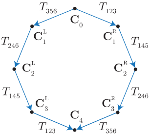
Figure 1: The graph of parametrisation charts

The parametrisation $C_{1}^{R}$, for example, corresponds to $\{x^{\prime}_{1},x^{\prime}_{2},x^{\prime}_{3},x_{4},x_{5},x_{6}\},$ and $C_{3}^{L}$ to $\{x_{1}^{*},x_{2}^{*},x_{3}^{*},x_{4}^{**},x_{5}^{**},x_{6}^{**}\}.$ The last parametrisations in both chains coincide due to the tetrahedron equation.

2.2 Involution and other orders

Recall that for the matrix ring with coefficients in the associative algebra there is the following homomorphism

$$\theta:Mat_{n}(\mathcal{A})\rightarrow Mat_{n}(\mathcal{A}^{op});\qquad\theta(M)^{i}_{j}=M^{n-j+1}_{n-i+1};$$

this is the reflection of the matrix with respect to the antidiagonal. It should also be noted that $\mathcal{A}^{op}$ is the same vector space as the algebra $\mathcal{A}$, but with inverse multiplication:

$$a\circ_{op}b=b\circ a.$$

We apply the homomorphism $\theta$ to the left-hand side of the tetrahedron equation (13)

$$\theta(M) = u_{12}(x_{6})u_{13}(x_{5})u_{14}(x_{4})u_{23}(x_{3})u_{24}(x_{2})u_{34}(x_{1})$$ (15)

$$= u_{12}(x_{6})u_{13}(x_{5})u_{14}(x_{4})u_{34}(x^{\prime}_{1})u_{24}(x^{\prime}_{2})u_{23}(x^{\prime}_{3})$$

$$= u_{12}(x_{6})u_{34}(x^{\prime\prime}_{1})u_{14}(x^{\prime}_{4})u_{13}(x^{\prime}_{5})u_{24}(x^{\prime}_{2})u_{23}(x^{\prime}_{3})$$

$$= u_{34}(x^{\prime\prime}_{1})u_{12}(x_{6})u_{14}(x^{\prime}_{4})u_{24}(x^{\prime}_{2})u_{13}(x^{\prime}_{5})u_{23}(x^{\prime}_{3})$$

$$= u_{34}(x^{\prime\prime}_{1})u_{24}(x^{\prime\prime}_{2})u_{14}(x^{\prime\prime}_{4})u_{12}(x^{\prime}_{6})u_{13}(x^{\prime}_{5})u_{23}(x^{\prime}_{3})$$

$$= u_{34}(x^{\prime\prime}_{1})u_{24}(x^{\prime\prime}_{2})u_{14}(x^{\prime\prime}_{4})u_{23}(x^{\prime\prime}_{3})u_{13}(x^{\prime\prime}_{5})u_{12}(x^{\prime\prime}_{6}).$$

Now let’s make a substitution:

$$\tau:x_{1}\leftrightarrow y_{6};~x_{2}\leftrightarrow y_{5};~x_{3}\leftrightarrow y_{3};~x_{4}\leftrightarrow y_{4};~x_{5}\leftrightarrow y_{2};~x_{6}\leftrightarrow y_{1}.$$ (16)

$$\tau\circ\theta(M) = u_{12}(y_{1})u_{13}(y_{2})u_{14}(y_{4})u_{23}(y_{3})u_{24}(y_{5})u_{34}(y_{6})$$ (17)

$$= u_{12}(y_{1})u_{13}(y_{2})u_{14}(y_{4})u_{34}(y^{\prime}_{6})u_{24}(y^{\prime}_{5})u_{23}(y^{\prime}_{3})$$

$$= u_{12}(y_{1})u_{34}(y^{\prime\prime}_{6})u_{14}(y^{\prime}_{4})u_{13}(y^{\prime}_{5})u_{24}(y^{\prime}_{5})u_{23}(y^{\prime}_{3})$$

$$= u_{34}(y^{\prime\prime}_{6})u_{12}(y_{1})u_{14}(y^{\prime}_{4})u_{24}(y^{\prime}_{5})u_{13}(y^{\prime}_{2})u_{23}(y^{\prime}_{3})$$

$$= u_{34}(y^{\prime\prime}_{6})u_{24}(y^{\prime\prime}_{5})u_{14}(x^{\prime\prime}_{4})u_{12}(y^{\prime}_{1})u_{13}(y^{\prime}_{2})u_{23}(x^{\prime}_{3})$$

$$= u_{34}(y^{\prime\prime}_{6})u_{24}(y^{\prime\prime}_{5})u_{14}(y^{\prime\prime}_{4})u_{23}(y^{\prime\prime}_{3})u_{13}(y^{\prime\prime}_{2})u_{12}(y^{\prime\prime}_{1}).$$

A similar expression for the right-hand side of the series of decompositions (14) takes the form

$$\tau\circ\theta(M) = u_{12}(y_{1})u_{13}(y_{2})u_{23}(y_{3})u_{14}(y_{4})u_{24}(y_{5})u_{34}(x_{6})$$ (18)

$$= u_{23}(y^{*}_{3})u_{24}(y^{*}_{2})u_{12}(y^{*}_{1})u_{14}(y_{4})u_{24}(y_{5})u_{34}(y_{6})$$

$$= u_{23}(y^{*}_{3})u_{13}(y^{*}_{2})u_{24}(y^{*}_{5})u_{14}(y^{*}_{4})u_{12}(y^{**}_{1})u_{34}(y_{6})$$

$$= u_{23}(y^{*}_{3})u_{24}(y^{*}_{5})u_{13}(y^{*}_{2})u_{14}(y^{*}_{4})u_{34}(y_{6})u_{12}(y^{**}_{1})$$

$$= u_{23}(y^{*}_{3})u_{24}(y^{*}_{5})u_{34}(y^{*}_{6})u_{14}(y^{**}_{4})u_{13}(y^{**}_{2})u_{12}(y^{**}_{1})$$

$$= u_{34}(y^{\prime\prime}_{6})u_{24}(y^{\prime\prime}_{5})u_{14}(y^{\prime\prime}_{4})u_{23}(y^{\prime\prime}_{3})u_{13}(y^{\prime\prime}_{2})u_{12}(x^{\prime\prime}_{1}).$$

These calculations imply that the charts corresponding to the 1st, 2nd, 3rd, 5th and 6th lines of the equations (17) and (18) are parametrisations in the spaces of unipotent matrices of the form

$$M^{\prime\prime}=\left(\begin{array}[]{cccc}1&y^{\prime\prime}_{1}&y^{\prime\prime}_{2}&y^{\prime\prime}_{4}\\ 0&1&y^{\prime\prime}_{3}&y^{\prime\prime}_{5}\\ 0&0&1&y^{\prime\prime}_{6}\\ 0&0&0&1\end{array}\right).$$ (23)

In this case, the transformations between the charts from top to bottom are now carried out by the maps $T_{ijk}$ themselves.

3 Quantisations of the unipotent groups

3.1 The case $N(3,A)$, classification of stable PBW ideals

Consider a free associative unital algebra $A=\mathbb{C}\left<x_{1},x_{2},x_{3}\right>$ and its automorphism $\operatorname{T}$, defined on generators by

$$\operatorname{T}:A\to A,\qquad\operatorname{T}(x_{1})=x_{1},\quad\operatorname{T}(x_{2})=x_{2}+x_{1}x_{3},\quad\operatorname{T}(x_{3})=x_{3}.$$ (24)

It is known [10] that this map $\operatorname{T}$ gives rise to a solution of the tetrahedron equation, analogous to the one in the commutative case.

By quantisation we mean the canonical reduction to a quotient algebra $A/I$ over a two sided $\operatorname{T}$–stable ideal $I\subset A$ , i.e. $\operatorname{T}(I)\subset I$, such that $A/I$ admits a basis

$$B=\langle{x}_{1}^{n}{x}_{2}^{m}{x}_{3}^{k}\,|\,n,m,k\in\mathbb{Z}_{\geqslant 0}\rangle$$ (25)

of normally ordered monomials. The ideal $I$ and quotient algebra $A/I$ are referred to as the quantisation ideal and the quantum algebra, respectively.

For brevity, we refer to normally ordered monomials as standard. Non-standard monomials can be expressed in terms of the standard monomial basis modulo the ideal. Equality modulo an ideal $I$ will be denoted by $\stackrel{{\scriptstyle I}}{{\equiv}}$, or simply $\equiv$ when the ideal under discussion is clear. A basis of normally ordered monomials (25) we refer as a Poincaré–Birkhoff–Witt or a PBW basis. An ideal $I\subset A$ we refer as a PBW ideal if the quotient algebra $A/I$ admits a PBW basis.

As a candidate for a quantisation ideal, we consider the ideal $I$ generated by the following three polynomials:

$$I=\langle F_{1}:=x_{2}x_{1}-f_{1},\ F_{2}:=x_{3}x_{1}-f_{2},\ F_{3}:=x_{3}x_{2}-f_{3}\rangle\,,$$ (26)

where $f_{k}$ are general quadratic non-homogeneous polynomials expressed in terms of normally ordered monomials as:

$$f_{k}=x_{1}^{2}\alpha_{k1}+x_{1}x_{2}\alpha_{k2}+x_{2}^{2}\alpha_{k3}+x_{1}x_{3}\alpha_{k4}+x_{2}x_{3}\alpha_{k5}+x_{3}^{2}\alpha_{k6}+x_{1}\beta_{k1}+x_{2}\beta_{k2}+x_{3}\beta_{k3}+\gamma_{k}\,,$$ (27)

with $\alpha_{ij},\beta_{ij},\gamma_{i}\in\mathbb{C}$ as arbitrary parameters. We further assume:

$$\alpha_{12}\neq 0,\quad\alpha_{24}\neq 0,\quad\alpha_{35}\neq 0.$$ (28)

The conditions for $\operatorname{T}$–stability of the ideal and the existence of the PBW basis in the quotient algebra $A/I$ impose constraints on these parameters.

Theorem 3.1.

An ideal $I$ (as defined in (26), (27), and (28)) is $\operatorname{T}$–stable and PBW if and only if it is generated by one of the following sets of polynomials:

Case 1:

$$\begin{array}[]{l}x_{2}\,x_{1}-x_{1}\,x_{2}-x_{1}^{2}\alpha_{11}-x_{1}\,x_{3}\alpha_{14}-x_{3}^{2}\alpha_{16}-x_{1}\beta_{11}-x_{3}\beta_{13}-\gamma_{1},\\ x_{3}\,x_{1}-x_{1}\,x_{3},\\ x_{3}\,x_{2}-x_{2}\,x_{3}-x_{1}^{2}\alpha_{31}-x_{1}\,x_{3}\alpha_{34}-x_{3}^{2}\alpha_{36}-x_{1}\beta_{31}-x_{3}\beta_{33}-\gamma_{3};\end{array}$$ (29)

Case 2:

$$\begin{array}[]{l}x_{2}\,x_{1}+x_{1}\,x_{2}-x_{1}^{2}\alpha_{11}-x_{3}^{2}\alpha_{16}-x_{3}\beta_{13}-x_{1}\beta_{33}-\gamma_{1},\\ x_{3}\,x_{1}+x_{1}\,x_{3},\\ x_{3}\,x_{2}+x_{2}\,x_{3}-x_{1}^{2}\alpha_{31}-x_{3}^{2}\alpha_{36}-x_{1}\beta_{31}-x_{3}\beta_{33}-\gamma_{3};\end{array}$$ (30)

Case 3:

$$\begin{array}[]{l}x_{2}\,x_{1}-\omega\,x_{1}\,x_{2}-x_{1}^{2}\alpha_{11}-x_{1}\beta_{33},\\ x_{3}\,x_{1}-\omega\,x_{1}\,x_{3},\\ x_{3}\,x_{2}-\omega\,x_{2}\,x_{3}-x_{3}^{2}\alpha_{36}-x_{3}\beta_{33},\end{array}$$ (31)

where $\alpha_{ij},\ \beta_{ij},\ \gamma_{i}$ and $\omega\neq 0$ are arbitrary parameters.

Remark 3.2.

.

• Cases 1, 2 can be viewed as a deformations of the commutative polynomial algebra $\mathbb{C}[x_{1},x_{2},x_{3}]$.

• Case 2 corresponds to a quantum algebra that has no commutative limit. It can be viewed as a deformation of the noncommutative algebra $\mathbb{C}\langle x_{1},x_{2},x_{3}\rangle/\langle x_{1}x_{2}+x_{2}x_{1},x_{1}x_{3}+x_{3}x_{1},x_{3}x_{2}+x_{2}x_{3}\rangle$. The associated Poisson structure can be constructed using the techniques developed in [9].

Proof: Our proof is based on two lemmas and Levandovskyy’s Theorem 2.3 [11]. Let us first assume that the quotient algebra $A/I$ admits the PBW basis (25) and find a general form of a $\operatorname{T}$–stable ideal. Then we will find and solve conditions for the existence of the PBW basis.

Lemma 3.3.

Let the standard monomials be linearly independent in $A/I$. Then a $\operatorname{T}$–stable ideal $I$ is generated by polynomials of the form

$$\begin{array}[]{l}x_{2}\,x_{1}-\omega x_{1}\,x_{2}-x_{1}^{2}\alpha_{11}-x_{1}\,x_{3}\alpha_{14}-x_{3}^{2}\alpha_{16}-x_{1}\beta_{11}-x_{3}\beta_{13}-\gamma_{1},\\ x_{3}\,x_{1}-\omega x_{1}\,x_{3},\\ x_{3}\,x_{2}-\omega x_{2}\,x_{3}-x_{1}^{2}\alpha_{31}-x_{1}\,x_{3}\alpha_{34}-x_{3}^{2}\alpha_{36}-x_{1}\beta_{31}-x_{3}\beta_{33}-\gamma_{3},\end{array}$$ (32)

where the coefficients $\alpha_{ij},\ \beta_{ij},\ \gamma_{i}$ and $\omega\neq 0$ are arbitrary parameters.

Proof of Lemma 3.3 The stability conditions $\operatorname{T}(F_{k})\stackrel{{\scriptstyle I}}{{\equiv}}0,\ k=1,2,3$ yield a system of polynomial equations for the coefficients of $F_{k}$. It follows from the form of polynomials $F_{k}$ that linear combinations of standard monomials do not belong to the ideal $I$. Consider

$$\operatorname{T}(F_{2})=F_{2}-x_{1}x_{3}x_{1}x_{3}\alpha_{23}-x_{1}^{2}x_{3}\alpha_{22}-x_{1}x_{3}x_{2}\alpha_{23}-x_{2}x_{1}x_{3}\alpha_{23}-x_{1}x_{3}^{2}\alpha_{25}-x_{1}x_{3}\beta_{22}.$$

Using the relation

$$x_{1}x_{3}x_{1}x_{3}\equiv x_{1}f_{1}x_{3}=\alpha_{24}x_{1}^{2}x_{3}^{2}+\cdots\gamma_{2}x_{1}x_{3}\not\in J,\quad\alpha_{24}\neq 0,$$

we conclude that $\operatorname{T}(F_{2})\in I$ implies

$$\alpha_{23}=\alpha_{22}=\alpha_{25}=\beta_{22}=0,$$

and thus

$$x_{3}x_{1}\equiv f_{2}=x_{1}x_{3}\alpha_{24}+x_{1}^{2}\alpha_{21}+x_{3}^{2}\alpha_{26}+x_{1}\beta_{21}+x_{3}\beta_{23}+\gamma_{2}.$$ (33)

Similarly, the conditions $\operatorname{T}(F_{1}),\operatorname{T}(F_{3})\in I$ imply

$$\alpha_{13}=\alpha_{33}=0,$$

and therefore

$$\operatorname{T}(F_{1})\equiv-x_{1}^{2}x_{3}\alpha_{1,2}-x_{1}x_{3}^{2}\alpha_{1,5}-x_{1}x_{3}\beta_{1,2}+x_{1}x_{3}x_{1},$$ (34)

$$\operatorname{T}(F_{3})\equiv-x_{1}^{2}x_{3}\alpha_{3,2}-x_{1}x_{3}^{2}\alpha_{3,5}-x_{1}x_{3}\beta_{3,2}+x_{3}x_{1}x_{3}.$$ (35)

We use $x_{1}x_{3}x_{1}\equiv x_{1}f_{2}$ and $x_{3}x_{1}x_{3}\equiv f_{2}x_{3}$ to present (34), (35) in the basis of standard monomials:

$$\begin{array}[]{l}\operatorname{T}(F_{1})\equiv x_{1}^{2}x_{3}\left(\alpha_{24}-\alpha_{12}\right)+x_{1}x_{3}^{2}\left(\alpha_{26}-\alpha_{15}\right)+x_{1}^{3}\alpha_{21}+x_{1}x_{3}\left(\beta_{23}-\beta_{12}\right)+x_{1}^{2}\beta_{21}+\gamma_{2}x_{1},\\ \operatorname{T}(F_{3})\equiv x_{1}^{2}x_{3}\left(\alpha_{21}-\alpha_{32}\right)+x_{1}x_{3}^{2}\left(\alpha_{24}-\alpha_{35}\right)+x_{3}^{3}\alpha_{26}+x_{1}x_{3}\left(\beta_{21}-\beta_{32}\right)+x_{3}^{2}\beta_{23}+\gamma_{2}x_{3}.\end{array}$$

Since we assume that the standard monomials are linearly independent, we get

$$\alpha_{12}=\alpha_{24}=\alpha_{35}:=\omega\neq 0,\quad\alpha_{15}=\alpha_{21}=\alpha_{26}=\alpha_{32}=\beta_{12}=\beta_{21}=\beta_{23}=\beta_{32}=\gamma_{2}=0.\qquad\Box$$

In algebra $A/I$ with $I$ generated by polynomials of the form (32) we can choose any ordering of the generators as a normal ordering. Moreover, the conditions for the existence of a PBW basis do not depend on the ordering.

Lemma 3.4.

Let an ideal $I\subset A$ be generated by polynomials (32) and $\omega\neq 0$. Then the quotient algebra $A/I$ admits a PBW basis $B=\langle{x}_{1}^{n}{x}_{2}^{m}{x}_{3}^{k}\,|\,n,m,k\in\mathbb{Z}_{\geqslant 0}\rangle$ if and only if it admits a PBW basis $B_{\sigma}=\langle{x}_{\sigma(1)}^{n}{x}_{\sigma(2)}^{m}{x}_{\sigma(3)}^{k}\,|\,n,m,k\in\mathbb{Z}_{\geqslant 0}\rangle$, where $\sigma$ is any permutation of $\{1,2,3\}$.

To determine a criterion for the existence of a PBW basis, we will use Levandovskyy’s Theorem [11] (Theorem 2.3). To do so, we introduce the notations and definitions that will be used throughout this and subsequent sections of the paper.

Consider a free associative algebra $\mathcal{A}=\mathbb{C}\langle s_{1},\ldots,s_{n}\rangle$ with $n$ generators $s_{1},\ldots,s_{n}$. Let $\mathcal{M}$ denote the set of all monomials in $\mathcal{A}$. Define the set of standard monomials

$$\mathcal{B}=\{s_{1}^{\alpha_{1}}s_{2}^{\alpha_{2}}\cdots s_{n}^{\alpha_{n}}\,|\,(\alpha_{1},\alpha_{2},\ldots,\alpha_{n})\in\mathbb{Z}_{\geqslant 0}^{n}\}$$ (36)

and let $L_{\mathcal{B}}=\operatorname{span}_{\mathbb{C}}(\mathcal{B})$ denotes the $\mathbb{C}$–linear space spanned by the standard monomials. Two monomials $a,b\in\mathcal{A}$ are said to be similar $a\sim b$ if $b$ can be obtained from $a$ by a permutation of letters (e.g. $s_{1}^{2}s_{3}\not\sim s_{1}s_{2}s_{3}\sim s_{3}s_{2}s_{1}\sim s_{2}s_{1}s_{3}$). There is a projection $\pi_{0}:\,\mathcal{M}\mapsto\mathcal{B}$ defined by the condition $\pi_{0}(a)=\pi_{0}(b)\,\Leftrightarrow\,a\sim b$.

Definition 3.5.

From this point onward, we fix the following monomial ordering $\prec$ on $\mathcal{M}$: the generators are ordered as $s_{1}\prec\cdots\prec s_{n}$. For standard monomials, we use the reverse (right) lexicographical order. Namely, $s_{1}^{\alpha_{1}}\cdots s_{n}^{\alpha_{n}}\prec s_{1}^{\beta_{1}}\cdots s_{n}^{\beta_{n}}$ if in the difference $(\beta_{1}-\alpha_{1},\ldots,\beta_{n}-\alpha_{n})$ the rightmost nonzero entry is positive. We extend it to $\mathcal{M}$ as following:

• $a\prec b$ if $\pi_{0}(a)\prec\pi_{0}(b)$;

• if $a\sim b$, we find their largest common left subword $m$ such that $a=ma_{1},\,b=mb_{1}$, or set $m=1$ if no such subword exists. Let $s_{i}$ and $s_{j}$ denote the first letters of $a_{1}$ and $b_{1}$, respectively (counting from the left). Then, $a\prec b$ if $s_{i}\prec s_{j}$.

In this ordering, standard monomials are the smallest within their equivalence classes of monomials. For example:

$$1\prec s_{1}\prec s_{1}^{2}\prec s_{2}\prec s_{1}s_{2}\prec s_{2}s_{1}\prec s_{2}^{2}\prec s_{3}\prec s_{1}s_{3}\prec s_{2}s_{3}\prec s_{1}s_{2}s_{3}\prec s_{2}s_{1}s_{3}\prec s_{3}s_{1}s_{2}\,.$$ (37)

Any non-zero $f\in\mathcal{A}$ can be written uniquely as $f=c\,m+f^{\prime}$, where $c\in\mathbb{C}^{*},\,m\in\mathcal{M}$ and $m^{\prime}\prec m$. We define $\operatorname{lm}(f):=m$ the leading monomial of $f$, and refer to the product $c\,m$ as the leading term of $f$. Suppose we have a set of $n(n-1)/2$ polynomials $f_{ij}$:

$$\begin{array}[]{lll}F&=&\{f_{ij}\,|\,1\leqslant i<j\leqslant n\}\subset\mathcal{A}=\mathbb{C}\langle s_{1},\ldots,s_{n}\rangle,\ \ \mbox{where}\\ &&\forall\,i<j\quad f_{ij}=s_{j}s_{i}-\omega_{ij}s_{i}s_{j}-d_{ij},\ \ \omega_{ij}\in\mathbb{C}^{*},\ \ d_{ij}\in L_{\mathcal{B}},\end{array}$$ (38)

such that

$$\operatorname{lm}(d_{ij})\prec s_{i}s_{j}\prec\operatorname{lm}(f_{ij})=s_{j}s_{i}.$$ (39)

In the polynomials $f_{ij}$, all monomials, except the leading monomial $s_{j}s_{i}$, are normally ordered (standard). Also we consider only homogeneous quadratic polynomials $d_{ij}$.

Any element $a\in\mathcal{A}$ can be brought to normally ordered form modulo the set of polynomials $F$. Indeed, let $m$ be the leading non-standard monomial in $a$. Since $m$ is non-standard, it must contain a pair of generators $s_{i}s_{j}$ appearing in the wrong order (i.e., with $i<j$). Thus, we can write $m=ps_{j}s_{i}q$, where $p,q$ are monomials. We rewrite this as $m=p(s_{j}s_{i}-f_{ij})q+pf_{ij}q$. By construction, the leading monomial of $\operatorname{lm}(p(s_{j}s_{i}-f_{ij})q)$ is strictly smaller than $m$ with respect to the monomial order $\prec$. Since the number of monomials of a fixed grading is finite, the process of reordering terminates after finitely many steps. As a result, we can express $a$ as $a=(:a:)+\tilde{a}$, where $(:a:)\in L_{\mathcal{B}}$ is a normally ordered polynomial (i.e., a linear combination of standard monomials), and the remainder $\tilde{a}$ is a finite sum of the form $\tilde{a}=\sum\limits_{k}\sum\limits_{1\leqslant i<j\leqslant n}p_{kij}f_{ij}q_{kij},\ \ p_{kij},\,q_{kij}\in\mathcal{A}$. In other words, treating the relations $f_{ij}\stackrel{{\scriptstyle\left<F\right>}}{{\equiv}}0$ as rewriting rules, we can transform any element $a\in\mathcal{A}$ into a normally ordered form $(:a:)$ in a finite number of steps.

In general, the normally ordered form of an element $a\in\mathcal{A}$ is not uniquely defined unless additional conditions are imposed on the coefficients of the polynomials $f_{ij}$. These conditions are well known - see for example Theorem 2.1 in [12]. Here we will use Levandovskyy’s Theorem [11] (Theorem 2.3), which we have adapted to suit our notations.

Theorem 3.6.

Let $\mathcal{I}=\langle F\rangle\subset\mathcal{A}$ be the two–sided ideal generated by a set of polynomials $F$ (38) satisfying conditions (39). Then, the following conditions are equivalent:

1. The quotient $\mathbb{C}$–algebra $\mathcal{A}/\mathcal{I}$ has a Poincaré–Birkhoff–Witt basis $\mathcal{B}$;

2. $F$ is a Gröbner basis for $\mathcal{I}$ with respect to the ordering $\prec$;

3. For all $1\leqslant i<j<k\leqslant n$,

   $$\Delta_{kji}=(:\,(:s_{k}\,s_{j}:)\,s_{i}:)-(:s_{k}\,(:s_{j}\,s_{i}:):)=0.$$ (40)

In particular, the conditions (40) are necessary and sufficient for the linear independence of standard monomials in the quotient algebra $\mathcal{A}/\mathcal{I}$. These conditions ensure the uniqueness of normally ordered forms.

We can use the above result to find necessary and sufficient conditions for the existence of a PBW basis of the quotient algebra $A/I$ in the case of ideals $I$ generated by polynomials (32). Let us consider the algebra $A=\mathbb{C}\langle s_{1},s_{2},s_{3}\rangle$ and identify the variables $s_{i}$ with $x_{i}$ as

$$s_{1}=x_{1},\quad s_{2}=x_{3},\quad s_{3}=x_{2}.$$ (41)

Then the ideal $I\subset A$ is generated by the polynomials

$$\begin{array}[]{l}f_{12}=s_{2}\,s_{1}-\omega s_{1}\,s_{2},\\ f_{13}=s_{3}\,s_{1}-\omega s_{1}\,s_{3}-s_{1}^{2}\alpha_{11}-s_{1}\,s_{2}\alpha_{14}-s_{2}^{2}\alpha_{16}-s_{1}\beta_{11}-s_{2}\beta_{13}-\gamma_{1},\\ f_{23}=s_{3}\,s_{2}-\omega^{-1}s_{2}\,s_{3}+\omega^{-1}(s_{1}^{2}\alpha_{31}+s_{1}\,s_{2}\alpha_{34}+s_{2}^{2}\alpha_{36}+s_{1}\beta_{31}+s_{2}\beta_{33}+\gamma_{3}).\end{array}$$ (42)

Conditions (39) are clearly satisfied (see (37)):

$$s_{1}s_{2}\prec s_{2}s_{1},\quad s_{2}^{2}\prec s_{1}s_{3}\prec s_{3}s_{1},\quad s_{2}^{2}\prec s_{2}s_{3}\prec s_{3}s_{2}.$$

In the case $n=3$, there is only one equation (40)

$$\Delta_{321}=(:\,(:s_{3}\,s_{2}:)\,s_{1}:)-(:s_{3}\,(:s_{2}\,s_{1}:):)=0,$$

which must be satisfied. It follows from

$$\begin{array}[]{lcl}(:\,(:s_{3}\,s_{2}:)\,s_{1}:)&=&s_{1}\,s_{2}\left(\beta_{11}-\beta_{33}\right)+s_{1}^{2}\,s_{2}\left(\omega\alpha_{11}-\alpha_{34}\right)+{s_{2}^{2}\beta_{13}}{\omega^{-1}}+s_{1}\,s_{2}^{2}\left(\alpha_{14}-\omega\alpha_{36}\right)\\ &+&{s_{2}^{3}\alpha_{16}}{\omega^{-1}}-{s_{1}^{3}\alpha_{31}}{\omega^{-1}}-{s_{1}^{2}\beta_{31}}{\omega^{-1}}+{\gamma_{1}s_{2}}{\omega^{-1}}-{\gamma_{3}s_{1}}{\omega^{-1}}+s_{1}\,s_{2}\,s_{3}\omega,\\ &&\\ (:s_{3}\,(:s_{2}\,s_{1}:):)&=&s_{1}\,s_{2}\left(\omega\beta_{11}-\omega\beta_{33}\right)+s_{1}^{2}s_{2}\left(\omega\alpha_{11}-\omega\alpha_{34}\right)+s_{2}^{2}\omega\beta_{13}+s_{1}\,s_{2}^{2}\left(\omega\alpha_{14}-\omega\alpha_{36}\right)\\ &+&s_{2}^{3}\omega\alpha_{16}-s_{1}^{3}\omega\alpha_{31}-s_{1}^{2}\omega\beta_{31}+\gamma_{1}s_{2}\omega-\gamma_{3}s_{1}\omega+s_{1}\,s_{2}\,s_{3}\omega,\end{array}$$

that

$$\begin{array}[]{lcl}\Delta_{321}&=&(\omega-1)\Big{(}s_{1}s_{2}\left(\beta_{33}-\beta_{11}\right)-s_{1}s_{2}^{2}\alpha_{14}+s_{1}^{2}s_{2}\alpha_{34}\Big{)}\\ &+&\omega^{-1}(1-\omega^{2})\Big{(}s_{2}^{2}\beta_{13}+s_{2}^{3}\alpha_{16}-s_{1}^{3}\alpha_{31}-s_{1}^{2}\beta_{31}+\gamma_{1}s_{2}-\gamma_{3}s_{1}\Big{)}=0.\end{array}$$

The above leads to three cases as stated in the theorem:

1. $\omega=1$, with no conditions on the other coefficients;

2. $\omega=-1$, with the conditions $\beta_{33}=\beta_{11}$ and $\alpha_{14}=\alpha_{34}=0$;

3. $\beta_{33}=\beta_{11}$ and $\alpha_{14}=\alpha_{34}=\beta_{13}=\alpha_{16}=\alpha_{31}=\beta_{31}=\gamma_{1}=\gamma_{3}=0$. $\Box$

Remark 3.7.

The identification (41) defines the monomial ordering in $A$, such that the ideal $I$ in Lemma 3.3 is generated by polynomials satisfying to the conditions (38), (39). Moreover, with this ordering, the leading term of any element $a\in A$ is $\operatorname{T}$–stable as $\operatorname{lm}(\operatorname{T}(a))=\operatorname{lm}(a)$. The algebra $A$ with the ideal $I$ also admits a different monomial ordering, corresponding to the identification

$$\hat{s}_{1}=x_{3},\qquad\hat{s}_{2}=x_{1},\qquad\hat{s}_{3}=x_{2},$$ (43)

which similarly satisfies the above properties. This alternative monomial ordering corresponds to the involution introduced in Section 2.2 which correspond to reflecting the matrix in (7) across its antidiagonal. $\Box$

3.2 The case $N(4,\mathcal{A})$, partial classification of quantisation ideals

Our main task is to describe the quantisation ideals of the free associative algebra $\mathcal{A}=\mathbb{C}\left<x_{1},\ldots,x_{6}\right>$ such that the maps $\operatorname{T}_{ijk}$ defined as $\operatorname{T}$ on the corresponding components

$$\operatorname{T}_{ijk}(x_{l})=\begin{cases}x_{j}+x_{i}x_{k},l=j,\\ x_{l},l\neq j.\end{cases}$$ (44)

act as automorphisms. In fact, we will consider only those maps that appear in the Zamolodchikov equation

$$T_{123}\circ T_{145}\circ\operatorname{T}_{246}\circ\operatorname{T}_{356}=\operatorname{T}_{356}\circ\operatorname{T}_{246}\circ T_{145}\circ T_{123}.$$ (45)

Due to the fact that $\operatorname{T}_{ijk}$ are homomorphisms of the free associative algebra by definition, we conclude that it is sufficient to check the identity (45) only on the generators of the algebra $x_{1},\ldots,x_{6}$. Checking the equality (45) turns out to be non-trivial only for $x_{4}$

$$\operatorname{LHS}(x_{4})=\operatorname{RHS}(x_{4})=x_{4}+x_{1}x_{5}+x_{1}x_{3}x_{6}+x_{2}x_{6}.$$

We adapt the notation from the previous chapter, namely, we introduce generators of the tensor algebra $\mathcal{A}=\mathbb{C}\left<s_{1},\ldots,s_{6}\right>$ with the monomial ordering described above (37) due to the identification

$$s_{1}=x_{1},s_{2}=x_{3},s_{3}=x_{2},s_{4}=x_{6},s_{5}=x_{5},s_{6}=x_{4}.$$ (46)

Moving to variables $s_{i}$, it is convenient to change notations for the maps $\operatorname{T}_{ijk}$ in order to make them consistent with the indices: $\Phi_{132}=\operatorname{T}_{123},\Phi_{165}=\operatorname{T}_{145},\Phi_{364}=\operatorname{T}_{246},\Phi_{254}=\operatorname{T}_{356}$. For example

$$\Phi_{132}(s_{3}) = s_{3}+s_{1}s_{2}=\operatorname{T}_{123}(x_{2})=x_{2}+x_{1}x_{3},$$

$$\Phi_{165}(s_{6}) = s_{6}+s_{1}s_{5},\ \ \,\Phi_{364}(s_{6})=s_{6}+s_{3}s_{4},$$

$$\Phi_{254}(s_{5}) = s_{5}+s_{2}s_{4}.$$

Thus

$$\Phi_{ijk}(s_{l})=\begin{cases}s_{j}+s_{i}s_{k},l=j,\\ s_{l},l\neq j.\end{cases}$$ (47)

We introduce the set of admissible triples of indices $S=\{(1,3,2),(1,6,5),(3,6,4),(2,5,4)\}$ which correspond to the homomorphisms $\Phi_{ijk}$ that occur in the tetrahedron equation.

Recall that $\mathcal{M}$ denotes the set of all monomials in the free algebra $\mathcal{A}$, and that $\mathcal{B}$ refers to the set of standard monomials defined in (36). The map $\operatorname{lm}:\mathcal{A}\to\mathcal{M}$ assigns to each element of $\mathcal{A}$ its leading monomial with respect to the monomial ordering $\prec$ introduced in Definition 3.5.

Lemma 3.8.

For any $a\in\mathcal{M}$ and any admissible triple $(i,j,k)\in S$, $\operatorname{lm}(\Phi_{ijk}(a))=a$

Proof.

It is true that $\operatorname{lm}(ab)=\operatorname{lm}(a)\operatorname{lm}(b)$, $\Phi_{ijk}(ab)=\Phi_{ijk}(a)\Phi_{ijk}(b)$, so it suffices to prove the statement for $a=s_{1},\ldots,s_{6}$. Note that $s_{i}s_{k}\prec s_{j}$, since $k<j$ for $(i,j,k)\in S$, then

$$\operatorname{lm}(\Phi_{ijk}(s_{l}))=\operatorname{lm}(s_{l}+\delta_{l,j}s_{i}s_{k})=s_{l},$$

where $\delta_{l,j}$ is the Kronecker delta. ∎

We begin the classification by studying ideals of toric type, denoted by $\mathcal{I}_{g}$, which are generated by relations of the form

$$g_{ij}=s_{j}s_{i}-\omega_{ij}s_{i}s_{j},\quad\omega_{ji}=\omega_{ij}^{-1},$$ (48)

and are $\Phi$-stable, that is, invariant under the automorphisms $\Phi_{i,j,k}$ for all $(i,j,k)\in S$.

Note that $\mathcal{I}_{g}$ automatically satisfies the PBW condition; thus, we only need to verify its stability. Theorem 3.1 implies that several of the parameters must coincide:

$$\begin{array}[]{ll}\Phi_{132}:\ \ \omega_{1}:=\omega_{12}=\omega_{13}=\omega_{32},&\Phi_{165}:\ \ \omega_{2}:=\omega_{15}=\omega_{16}=\omega_{65},\\ \Phi_{364}:\ \ \omega_{3}:=\omega_{34}=\omega_{36}=\omega_{64},&\Phi_{254}:\ \ \omega_{4}:=\omega_{24}=\omega_{25}=\omega_{54}.\end{array}$$ (49)

We introduce the shorthand notation $\omega_{1},\ldots,\omega_{4}$ for simplicity. These parameters correspond to the automorphisms $\Phi_{i,j,k},\ (i,j,k)\in S$. The remaining parameters $\omega_{14},\omega_{26},\omega_{35}$ correspond to index pairs that do not simultaneously appear in any triple from $S$.

Lemma 3.9.

A $\Phi$-stable ideal of the form (48) is uniquely determined by four parameters $\omega_{1},\omega_{2},\omega_{3},\omega_{4}$ satisfying the relation

$$\omega_{1}\omega_{3}=\omega_{2}\omega_{4}.$$ (50)

In this case, the parameters associated with the triplets in the tetrahedron equation are determined by the values of $\omega_{i}$ as specified in (49), while the remaining parameters are given by:

$$\omega_{14}=\omega_{2}/\omega_{1},\qquad\omega_{26}=\omega_{3}/\omega_{2},\qquad\omega_{35}=\omega_{2}\omega_{4}.$$ (51)

Proof.

Let $(i,j,k)\in S$ be any admissible triple, and let $r\notin\{i,j,k\}.$ We apply $\Phi_{ijk}$ to the generators of the ideal (48):

$$\Phi_{ijk}(g_{jr}) = (\omega_{ir}\omega_{kr}-\omega_{jr})s_{i}s_{k}s_{r}{\color[rgb]{0,0,1}+g_{jr}+g_{ir}s_{k}+\omega_{ir}s_{i}g_{kr};}$$

$$\Phi_{ijk}(g_{ij}) = (\omega_{ik}-\omega_{ij})s_{i}^{2}s_{k}{\color[rgb]{0,0,1}+g_{ij}+s_{i}g_{ik};}$$

$$\Phi_{ijk}(g_{kj}) = s_{i}s_{k}^{2}(1-\omega_{kj}\omega_{ik}){\color[rgb]{0,0,1}+g_{kj}-\omega_{kj}g_{ik}s_{k};}$$ (52)

(the terms from the ideal are marked in blue). Using the PBW property of this ideal, we obtain, in addition to the conditions formulated in Theorem 3.1, the following set of equations:

$$\begin{array}[]{llll}\omega_{12}\omega_{14}=\omega_{15},&\omega_{13}\omega_{14}=\omega_{16},&\omega_{24}=\omega_{26}\omega_{32},&\omega_{25}=\omega_{12}\omega_{26},\\ \omega_{14}\omega_{24}=\omega_{34},&\omega_{15}\omega_{25}=\omega_{35},&\omega_{34}\omega_{32}=\omega_{35},&\omega_{16}\omega_{26}=\omega_{36},\\ \omega_{35}=\omega_{13}\omega_{36},&\omega_{64}=\omega_{1,4}\omega_{54},&\omega_{26}\omega_{65}=\omega_{64},&\omega_{54}\omega_{65}=\omega_{35}.\end{array}$$

These 12 equations can be written uniformly as

$$\omega_{ni}\omega_{nk}=\omega_{nj},\qquad(i,j,k)\in S,\ \ n\not\in(i,j,k),$$

and represented by the diagram in the figure

The commutativity of the diagram guarantees the possibility of restoring all the parameters of the ideal from four $\omega_{1},\omega_{2},\omega_{3},\omega_{4}$ if the following is satisfied

$$\omega_{1}\omega_{3}=\omega_{2}\omega_{4}.$$

∎

Further on we will refer to invariant toric ideal as $I_{0}$ given by parameters $\omega_{1},\omega_{2},\omega_{3},\omega_{4}$ subject to the relation $\omega_{1}\omega_{3}=\omega_{2}\omega_{4}$.

We call a homogeneous quadratic ideal $\mathcal{I}\subset\mathcal{A}$ triangular if it is generated by polynomials of the form

$$f_{ij}:=g_{ij}-d_{ij};1\leqslant i<j\leqslant 6,$$ (53)

where

$$g_{ij}=s_{j}s_{i}-\omega_{ij}s_{i}s_{j},\qquad d_{ij}=\sum\limits_{(k,l)<(i,j),\,k\leqslant l}\delta_{ijkl}s_{k}s_{l}.$$

Here, $(k,l)<(i,j)$ denotes comparison in the right lexicographic order. This means that all monomials appearing in the quadratic polynomial $d_{ij}$ are standard, and that $\operatorname{lm}(d_{ij})\prec s_{i}s_{j}$.

The toric component of an arbitrary triangular $\Phi$-stable ideal satisfy the same equations as listed in Lemma 3.9.

Lemma 3.10.

Let a triangular ideal $\mathcal{I}$ be $\Phi$-stable and PBW, then parameters $\omega_{ij}$ satisfy the relations (49), (51) and (50).

Proof.

Note that due to the homogeneity of the ideal $\mathcal{I}$, the quotient algebra $\mathcal{A}/\mathcal{I}$ is graded. In addition, due to the PBW property, we have an isomorphism of graded vector spaces

$$\tau:\mathbb{C}[s_{1},\ldots,s_{6}]\rightarrow\mathcal{A}/\mathcal{I},$$

which is determined by the choice of the basis of ordered monomials. Consider the projection operator onto the degree three component

$$P_{3,\mathcal{A}/\mathcal{I}}:\mathcal{A}/\mathcal{I}\to(\mathcal{A}/\mathcal{I})_{3}.$$

This operator is consistent with the projection operator $P_{3,\mathcal{A}}$ in the free algebra $\mathcal{A}$

$$\pi P_{3,\mathcal{A}}=P_{3,\mathcal{A}/\mathcal{I}}\pi,$$

where $\pi:\mathcal{A}\to\mathcal{A}/\mathcal{I}$ is the canonical projection. From now on we will use the notation $P_{3}$ for both operators. Finally, we introduce the operator $\mathcal{P}_{3}=\tau^{-1}\circ P_{3}\circ\pi:\mathcal{A}\to(\mathbb{C}[s_{1},\ldots,s_{6}])_{3}$, which we will work with, and $\Pi=\tau^{-1}\circ\pi:\mathcal{A}\to\mathbb{C}[s_{1},\ldots,s_{6}]$. Recall that $\pi_{0}:\mathcal{M}\to\mathcal{B}$ is a map that, given an arbitrary monomial, constructs a standart monomial equivalent to it (in the sense of the introduced equivalence relation). Thanks to the relations (52) we can say that in the toric case

$$\mathcal{P}_{3}(\Phi_{ijk}(g_{ij}))\in\mathbb{C}\pi_{0}(s_{i}^{2}s_{k});\qquad\mathcal{P}_{3}(\Phi_{ijk}(g_{jr}))\in\mathbb{C}\pi_{0}(s_{i}s_{k}s_{r});\qquad\mathcal{P}_{3}(\Phi_{ijk}(g_{kj}))\in\mathbb{C}\pi_{0}(s_{i}s_{k}^{2}).$$

The relations of Lemma 3.9 guarantee the invariance of the ideal in the toric case. Now consider the invariance conditions for the general triangular ideal.

First of all, we note that the notion of a leading monomial on a free algebra for ideals of the type under consideration can be extended to the quotient algebra and coincides with the standard monomial $\operatorname{lm}(\Pi(a)))=\pi_{0}(a)$ for any monomial $a\in\mathcal{M}$ if we consider $\mathbb{C}[s_{1},\ldots,s_{6}]=\operatorname{span}_{\mathbb{C}}\mathcal{B}\subset\mathcal{A}$ as a vector space. In other words, the following diagram is commutative.

We prove that $\mathcal{P}_{3}(\Phi_{ijk}(d_{lj}))$ for $l<j$ does not contain the monomial $\pi_{0}(s_{i}s_{k}s_{l})$. This will mean that the condition on the coefficient of $\pi_{0}(s_{i}s_{k}s_{l})$ for a general ideal coincides with the condition for a toric one. To do this, we show that $\operatorname{lm}(P_{3}(\Phi_{ijk}(d_{lj})))\prec\pi_{0}(s_{i}s_{k}s_{l})$. In fact, let’s calculate the cubic part

$$\mathcal{P}_{3}(\Phi_{ijk}(\sum_{(p,q)<(l,j)}\delta_{ljpq}s_{p}s_{q}))=\mathcal{P}_{3}(\sum_{p<l}\delta_{ljpj}s_{p}s_{i}s_{k})=\mathcal{P}_{3}(\sum_{p<l}\delta_{ljpj}\pi_{0}(s_{p}s_{i}s_{k}))$$

It is enough to restrict the order to standard monomials of the same degree, that is, to consider the right (reverse) lexicographical ordering. We get

$$\operatorname{lm}(\mathcal{P}_{3}(\Phi_{ijk}(d_{lj})))\prec\pi_{0}(s_{i}s_{k}s_{l})$$

Let us carry out a similar argument to check that $\mathcal{P}_{3}(\Phi_{ijk}(d_{jr}))$ does not contain the monomial $\pi_{0}(s_{i}s_{k}s_{r})$ for $r>j$.

$$\operatorname{lm}(\mathcal{P}_{3}(\Phi_{ijk}(d_{jr})))\prec\pi_{0}(s_{i}s_{k}s_{r})$$

The cases $\mathcal{P}_{3}(\Phi_{ijk}(d_{ij}))$ and $\mathcal{P}_{3}(\Phi_{ijk}(d_{jk}))$ are checked similarly. The expressions $d_{l^{\prime}r^{\prime}}$ for $l^{\prime}\neq j$ and $r^{\prime}\neq j$ we have $\mathcal{P}_{3}(\Phi_{ijk}(d_{l^{\prime}r^{\prime}}))=0$, since $\Phi_{ijk}(d_{l^{\prime}r^{\prime}})$ does not contain cubic part. ∎

The following theorem provides a strong characterisation of triangular $\Phi$-stable ideals.

Theorem 3.11.

Let $\mathcal{I}$ be a triangular $\Phi$-stable PBW ideal, then $d_{ij}=0$ for $j<6$.

Proof.

(Sketch) Assume that the ideal $\mathcal{I}$ is $\Phi$-stable and satisfies the PBW condition. Then for each $(i,j,k)\in S$, we must have

$$\mathcal{P}_{3}(\Phi_{ijk}(f_{sp}))\equiv 0$$

The idea of the proof is to successively establish that each term $d_{ij}$ vanishes for $j<6$. The PBW condition, together with $\Phi$-invariance, imposes constraints on the coefficients $\delta_{ijkl}$ in the expressions for $d_{ij}$. At each step, we derive these constraints and observe that they reduce to trivial equations of the form $\delta_{ijkl}=0$, which can be solved recursively. This procedure eventually leads to the conclusion that all such correction terms must vanish.
Step 1.

By Lemma 3.10, the parameters $\omega_{ij}$ satisfy the necessary consistency conditions. Consider now the action of $\Phi_{132}$ on the generator $f_{13}$. We compute:

$$\mathcal{P}_{3}\left(\Phi_{132}(f_{13})\right)=s_{1}s_{2}s_{1}-\omega_{13}s_{1}^{2}s_{2}=(\omega_{12}-\omega_{13})s_{1}^{2}s_{2}+\delta_{1211}s_{1}^{3}.$$

Since the PBW condition requires $\mathcal{P}_{3}\left(\Phi_{132}(f_{13})\right)\equiv 0$, and by Lemma 3.10 we already know $\omega_{12}=\omega_{13}$, we conclude:

$$\delta_{1211}s_{1}^{3}=0\quad\Rightarrow\quad\delta_{1211}=0.$$

Therefore, the term $d_{12}$ vanishes, and the relation for $s_{2}s_{1}$ is purely of toric type.

This, in turn, implies that any terms involving $s_{3}$ appearing in $d_{ij}$ for $i,j\neq 3$ must vanish, i.e.,

$$\delta_{ijk3}=\delta_{ij3k}=0\quad\text{for all }i,j\neq 3.$$

Indeed:

$$\mathcal{P}_{3}(\Phi_{132}(f_{ij}))=\mathcal{P}_{3}(\Phi_{132}(\sum_{\begin{subarray}{c}p<3\\ (p,3)<(i,j)\end{subarray}}\delta_{ikp3}s_{p}s_{3}))+\mathcal{P}_{3}(\Phi_{132}(\sum_{\begin{subarray}{c}p>3\\ (3,p)<(i,j)\end{subarray}}\delta_{ij3p}s_{3}s_{p}))=$$

$$=\sum_{\begin{subarray}{c}p<3\\ (p,3)<(i,j)\end{subarray}}\delta_{ikp3}\pi(s_{p}s_{1}s_{2})+\sum_{\begin{subarray}{c}p>3\\ (3,p)<(i,j)\end{subarray}}\delta_{ij3p}s_{1}s_{2}s_{p}=$$

$$=\sum_{\begin{subarray}{c}p<3\\ (p,3)<(i,j)\end{subarray}}\delta_{ijp3}\omega_{1p}\pi_{0}(s_{p}s_{1}s_{2})+\sum_{\begin{subarray}{c}p>3\\ (p,3)<(i,j)\end{subarray}}\delta_{ij3p}s_{1}s_{2}s_{p}=0\implies\delta_{ij3p}=\delta_{ijp3}=0$$

The projection $\mathcal{P}_{4}$ onto monomials of degree 4 yields another relation, namely $\delta_{ij33}=0$. This follows because the only monomial of degree 4 appearing in the expression is

$$\delta_{ij33}\cdot\Pi(s_{1}s_{2}s_{1}s_{2})=\delta_{ij33}\omega_{12}s_{1}^{2}s_{2}^{2}.$$

Similarly, applying $\mathcal{P}_{4}$ to $\Phi_{254}(f_{ij})$ gives the relation

$$\delta_{ij55}=0.$$

Step 2.
It is not feasible to eliminate such a large number of coefficients through general reasoning alone. However, we will demonstrate the principle by which we proceed. As an illustration, we will show how to eliminate $d_{14}$ in two steps. We have:

$$\mathcal{P}_{3}(\Phi_{132}(f_{23}))=\Pi(s_{1}s^{2}_{2}-\omega_{23}s_{2}s_{1}s_{2}-\delta_{2313}s_{1}s_{1}s_{2})=(1-\omega_{23}\omega_{12})s_{1}s^{2}_{2}-\delta_{2313}s^{2}_{1}s_{2}\implies\delta_{2313}=0$$

$$\mathcal{P}_{3}(\Phi_{132}(f_{34}))=\Pi(s_{4}s_{1}s_{2}-\omega_{34}s_{1}s_{2}s_{4}-\delta_{3413}s^{2}_{1}s_{2}-\delta_{3423}s_{2}s_{1}s_{2})=$$

$$=\Pi(s_{4}s_{1}s_{2})-\omega_{34}s_{1}s_{2}s_{4}-\delta_{3413}s^{2}_{1}s_{2}-\delta_{3423}\omega_{12}s_{1}s^{2}_{2}$$

$$\Pi(s_{4}s_{1}s_{2})=\omega_{14}\omega_{24}s_{1}s_{2}s_{4}+(\delta_{1411}+\omega_{14}\delta_{2412})s^{2}_{1}s_{2}+(\delta_{1412}+\omega_{14}\delta_{2422})s_{1}s^{2}_{2}+$$

$$+\omega_{14}\delta_{2411}s^{3}_{1}+\delta_{1422}s^{3}_{2}+\omega_{14}\delta_{2414}s^{2}_{1}s_{4}$$

From the previous calculations, we observe that several coefficients in $d_{14}$ and $d_{24}$ vanish immediately, namely $\delta_{1422}=\delta_{2414}=\delta_{2411}=0$.

Next, a similar direct computation yields

$$\mathcal{P}_{3}(\Phi_{254}(f_{15}))=\omega^{2}_{12}\delta_{1411}s^{2}_{1}s_{2}+\omega_{12}\delta_{1412}s_{1}s^{2}_{2}\implies\delta_{1412}=\delta_{1411}=0$$

As a consequence, we obtain $d_{14}=0$.
Step 3.
Next, we show that $d_{24}=0$. We compute

$$\mathcal{P}_{3}(\Phi_{254}(f_{25}))=\omega_{12}\delta_{2412}s_{1}s^{2}_{2}+\delta_{2422}s^{3}_{2}-\delta_{2515}s_{1}s_{2}s_{4}.$$

We conclude that $\delta_{2412}=\delta_{2422}=\delta_{2515}=0$, and hence $d_{24}=0$.

Returning to the previous step, we also find that some of the remaining coefficient equations are now trivially satisfied, namely $\delta_{3423}=\delta_{3413}=0$.
Remaining steps.
We now indicate which automorphisms $\Phi_{ijk}$ should be applied to which generators $f_{kl}$ in order to deduce the vanishing of the remaining $d_{kl}$. As before, we resolve only trivial equations of the form $\delta_{ijkl}=0$ (using that $\omega_{ij}\neq 0$), and we also revisit previous coefficient equations since simplifications may occur.

$$\Phi_{254}(f_{35}),\Phi_{123}(f_{35}),\Phi_{165}(f_{16})\implies d_{15}=0$$

$$\Phi_{165}(f_{26})\implies d_{25}=0$$

$$\Phi_{165}(f_{36}),\Phi_{364}(f_{16})\implies d_{13}=0$$

$$\Phi_{364}(f_{26})\implies d_{23}=0$$

$$\Phi_{364}(f_{46})\implies d_{34}=d_{35}=0$$

$$\Phi_{132}(f_{45}),\Phi_{165}(f_{45}),\Phi_{165}(f_{56})\implies d_{45}=0$$

∎

Theorem 3.11 significantly simplifies the classification of triangular PBW ideals that are invariant under the automorphisms $\Phi_{ijk}$. It enables us to find the generators $f_{i,j}$ for the most general triangular ideal $I_{stab}$, that is, an ideal satisfying stability under all maps $\Phi_{ijk}$ but not necessarily the PBW property. The generators of the ideal are given by:

$$\begin{cases}f_{12}=s_{2}s_{1}-\omega_{1}s_{1}s_{2},\\ f_{13}=s_{3}s_{1}-\omega_{1}s_{1}s_{3},\\ f_{23}=s_{3}s_{2}-\omega_{1}^{-1}s_{2}s_{3},\\ f_{14}=s_{4}s_{1}-\omega_{2}\omega_{1}^{-1}s_{1}s_{4},\\ f_{24}=s_{4}s_{2}-\omega_{4}s_{2}s_{4},\\ f_{34}=s_{4}s_{3}-\omega_{3}s_{3}s_{4},\\ f_{15}=s_{5}s_{1}-\omega_{2}s_{1}s_{5},\\ f_{25}=s_{5}s_{2}-\omega_{4}s_{2}s_{5},\\ f_{35}=s_{5}s_{3}-\omega_{2}\omega_{4}s_{3}s_{5},\\ f_{45}=s_{5}s_{4}-\omega_{4}^{-1}s_{4}s_{5},\\ f_{16}=s_{6}s_{1}-\left(\omega_{2}s_{1}s_{6}+A_{3}s_{1}^{2}+A_{1}\omega_{1}s_{1}s_{2}+A_{2}s_{1}s_{4}\right),\\ f_{26}=s_{6}s_{2}-\left(\omega_{3}\omega^{-1}_{2}s_{2}s_{6}+A_{4}s_{1}s_{2}+A_{6}\omega_{1}s_{2}^{2}+A_{5}\omega_{4}s_{2}s_{4}\right),\\ f_{36}=s_{6}s_{3}-\left(\omega_{3}s_{3}s_{6}+A_{10}s_{1}^{2}+A_{7}s_{1}s_{2}+\left(A_{4}\omega_{2}+A_{3}\right)s_{1}s_{3}+A_{8}s_{1}s_{4}\right)-\\ \qquad-\left(A_{11}s_{2}^{2}+s_{2}s_{3}\left(A_{6}\omega_{2}+A_{1}\right)+A_{9}s_{2}s_{4}+\omega_{4}s_{3}s_{4}\left(A_{5}\omega_{2}+A_{2}\right)+A_{12}s_{4}^{2}\right),\\ f_{46}=s_{6}s_{4}-\left(\omega^{-1}_{3}s_{4}s_{6}+A_{13}s_{1}s_{4}+A_{14}\omega_{2}s_{2}s_{4}+A_{15}\omega_{1}s_{4}^{2}\right),\\ f_{56}=s_{6}s_{5}-\left(\omega^{-1}_{2}s_{5}s_{6}+A_{19}s_{1}^{2}+A_{16}s_{1}s_{2}+A_{17}s_{1}s_{4}+\left(A_{13}\omega_{4}+A_{4}\right)s_{1}s_{5}\right)-\\ \qquad-\left(A_{20}s_{2}^{2}+A_{18}s_{2}s_{4}+\left(A_{6}\omega_{1}+A_{14}\omega_{3}\right)s_{2}s_{5}+A_{21}s_{4}^{2}+\left(A_{5}+A_{15}\right)s_{4}.s_{5}\right)\end{cases}$$ (54)

In this system, all parameters $\omega_{i}$ and $A_{i}$ are arbitrary, except for the constraint $\omega_{1}\omega_{3}=\omega_{2}\omega_{4}$.

It follows from Theorem 3.6 that the ideal $I_{stab}$ is PBW if and only if

$$\big{(}:\,(:s_{k}\,s_{j}:)\,s_{i}:\big{)}=\big{(}:s_{k}\,(:s_{j}\,s_{i}:):\big{)},\qquad 1\leqslant i<j<k\leqslant 6.$$ (55)

Conditions (55) yield a system of 78 linear homogeneous equations for the unknowns $A_{1},\ldots,A_{21}$, with coefficients in the ring $\mathbb{Z}[\omega_{i},\omega_{i}^{-1}\,;\,i=1,\ldots,4]/(\omega_{1}\omega_{3}-\omega_{2}\omega_{4})$. The solvability conditions for this system impose polynomial constraints on the toric parameters $\omega_{i}$. The solution set defines an affine variety with several irreducible components. A complete classification of all solutions is challenging and currently beyond our reach.

In this paper, we focus on the generic case, where none of the parameters $\omega_{i}$ is identically equal to $\pm 1$. The generic case can be reduced to the following four subcases:

Case 1 $$:\qquad \omega_{1}\omega_{3}=\omega_{2}\omega_{4},$$ (56)

Case 2 $$:\qquad \omega_{1}=\omega_{2}=\omega_{3}=\omega_{4},$$ (57)

Case 3 $$:\qquad \omega_{1}=\omega_{2},\quad\omega_{3}=\omega_{4}=\omega_{2}^{2},$$ (58)

Case 4 $$:\qquad \omega_{1}=\omega_{2}=\omega_{4}^{2},\quad\omega_{3}=\omega_{4}.$$ (59)

Below we present generating polynomials for the most general $\Phi$-stable and PBW ideals corresponding to each Case.For brevity, we show only the polynomials $f_{i,j},\ j=6$; the generators $f_{i,j}$ with $j<6$ are all toric and given by (54) specialized to each case. The arbitrary constants $b_{i},C_{i}$ appearing here are related to, but do not coincide with, the constants $A_{i}$ in (54).

Toric ideal $I_{0}$:
Let $I_{0}$ denote a $\Phi$-stable ideal generated by the polynomials $g_{i,j}$ defined in (48), with the parameters $\omega_{i,j}$ specified in Lemma 3.9:

$$\left\{\begin{array}[]{lll}g_{12}=s_{2}s_{1}-\omega_{1}s_{1}s_{2},&g_{13}=s_{3}s_{1}-\omega_{1}s_{1}s_{3},&g_{23}=s_{3}s_{2}-\omega_{1}^{-1}s_{2}s_{3},\\ g_{14}=s_{4}s_{1}-\omega_{2}\omega_{1}^{-1}s_{1}s_{4},&g_{24}=s_{4}s_{2}-\omega_{1}\omega_{3}\omega_{2}^{-1}s_{2}s_{4},&g_{34}=s_{4}s_{3}-\omega_{3}s_{3}s_{4},\\ g_{15}=s_{5}s_{1}-\omega_{2}s_{1}s_{5},&g_{25}=s_{5}s_{2}-\omega_{1}\omega_{3}\omega_{2}^{-1}s_{2}s_{5},&g_{35}=s_{5}s_{3}-\omega_{1}\omega_{3}s_{3}s_{5},\\ g_{45}=s_{5}s_{4}-\omega_{2}\omega_{1}^{-1}\omega_{3}^{-1}s_{4}s_{5},&g_{16}=s_{6}s_{1}-\omega_{2}s_{1}s_{6},&g_{26}=s_{6}s_{2}-\omega_{3}\omega^{-1}_{2}s_{2}s_{6},\\ g_{36}=s_{6}s_{3}-\omega_{3}s_{3}s_{6},&g_{46}=s_{6}s_{4}-\omega^{-1}_{3}s_{4}s_{6},&g_{56}=s_{6}s_{5}-\omega^{-1}_{2}s_{5}s_{6}.\end{array}\right.$$ (60)

This ideal is parametrised by three independent non-zero parameters $\omega_{1},\omega_{2}$ and $\omega_{3}$.

Ideal $I_{1}$:
Case 1 yields the ideal $I_{1}$, generated by polynomials $f_{i,j}=g_{i,j},j<6$ (60), and:

$$\begin{cases}f_{16}=s_{6}s_{1}-\left(\omega_{2}s_{1}s_{6}+b_{1}\left(1-\omega_{2}\right)s_{1}^{2}+b_{2}\left(\omega_{1}-\omega_{2}\right)s_{1}s_{2}+b_{3}(\omega^{-1}_{1}-1)\omega_{2}\omega_{3}s_{1}s_{4}\right),\\ f_{26}=s_{6}s_{2}-\left(\omega_{3}\omega^{-1}_{2}s_{2}s_{6}+b_{1}(1-\omega_{1}\omega_{3}\omega^{-1}_{2})s_{1}s_{2}+b_{2}(1-\omega_{3}\omega^{-1}_{2})s^{2}_{2}+b_{3}(\omega_{1}-1)\omega^{2}_{3}\omega^{-1}_{2}s_{2}s_{4}\right),\\ f_{36}=s_{6}s_{3}-\left(\omega_{3}s_{3}s_{6}+b_{1}\left(1-\omega_{1}\omega_{3}\right)s_{1}s_{3}+b_{2}(1-\omega_{3}\omega^{-1}_{1})s_{2}s_{3}\right),\\ f_{46}=s_{6}s_{4}-\left(\omega^{-1}_{3}s_{4}s_{6}+b_{1}(1-\omega_{2}\omega^{-1}_{1}\omega^{-1}_{3})s_{1}s_{4}+b_{2}(1-\omega_{1}\omega^{-1}_{2})s_{2}s_{4}+b_{3}\left(\omega_{3}-1\right)s_{4}^{2}\right),\\ f_{56}=s_{6}s_{5}-\left(\omega^{-1}_{2}s_{5}s_{6}+b_{2}(1-\omega_{1}\omega_{3}\omega^{-2}_{2})s_{2}s_{5}+b_{3}(\omega_{3}-\omega^{-1}_{1})s_{4}s_{5}\right),\end{cases}$$ (61)

where $b_{1},b_{2},b_{3}$ and $\omega_{1},\omega_{2},\omega_{3}$ are arbitrary parameters.

Remark 3.12.

Ideal $I_{1}$ is a deformation of the generic toric ideal $I_{0}$, it coincides with $I_{0}$ if $b_{i}=0$.

Ideal $I_{2}$:
Case 2 yields the ideal $I_{2}$, generated by polynomials $f_{i,j}=g_{i,j},j<6$ (60), where $\omega_{1}=\omega_{2}=\omega_{3}=\omega$ and

$$\begin{cases}f_{16}=s_{6}s_{1}-\left(\omega s_{1}s_{6}-C_{5}\omega^{2}s_{1}s_{4}+C_{1}\omega s_{1}^{2}+\left(C_{3}-C_{2}\right)\omega s_{1}s_{2}\right),\\ f_{26}=s_{6}s_{2}-\left(s_{2}s_{6}+C_{5}\omega^{2}s_{2}s_{4}+C_{1}\omega s_{1}s_{2}+C_{2}s_{2}^{2}\right),\\ f_{36}=s_{6}s_{3}-\left(\omega s_{3}s_{6}+C_{1}\omega\left(\omega+1\right)s_{1}s_{3}+C_{3}s_{2}s_{3}\right),\\ f_{46}=s_{6}s_{4}-\left(\omega^{-1}s_{4}s_{6}+C_{5}\omega s_{4}^{2}-C_{1}s_{1}s_{4}+C_{4}s_{2}s_{4}\right),\\ f_{56}=s_{6}s_{5}-\left(\omega^{-1}s_{5}s_{6}+C_{5}\left(\omega+1\right)s_{4}s_{5}+\left(C_{2}+C_{4}\right)s_{2}s_{5}\right),\end{cases}$$ (62)

This ideal depends on arbitrary parameters $C_{1},C_{2},C_{3},C_{4},C_{5}$ and $\omega\neq 0$.

Ideal $I_{3}$:
Case 3 yields the ideal $I_{3}$, generated by polynomials $f_{i,j}=g_{i,j},j<6$ (60), where $\omega_{1}=\omega_{2}=\omega,\ \omega_{3}=\omega^{2}$ and

$$\begin{cases}f_{16}=s_{6}s_{1}-\left(\omega s_{1}s_{6}+C_{1}\omega^{2}s_{1}^{2}+C_{2}\omega^{3}s_{1}s_{4}\right),\\ f_{26}=s_{6}s_{2}-\left(\omega s_{2}s_{6}+C_{1}\left(\omega+1\right)\omega^{2}s_{1}s_{2}+C_{4}s_{2}^{2}-C_{2}\omega^{4}s_{2}s_{4}\right),\\ f_{36}=s_{6}s_{3}-\left(\omega^{2}s_{3}s_{6}+C_{1}\left(\omega^{2}+\omega+1\right)\omega^{2}s_{1}s_{3}+C_{3}s_{2}^{2}+C_{4}s_{2}s_{3}\right),\\ f_{46}=s_{6}s_{4}-\left(\omega^{-2}s_{4}s_{6}-C_{1}\left(\omega+1\right)s_{1}s_{4}-C_{2}\left(\omega+1\right)\omega s_{4}^{2}\right),\\ f_{56}=s_{6}s_{5}-\left(\omega^{-1}s_{5}s_{6}+C_{4}s_{2}s_{5}-C_{2}\left(\omega^{2}+\omega+1\right)s_{4}s_{5}\right),\end{cases}$$ (63)

This ideal depends on arbitrary parameters $C_{1},C_{2},C_{3},C_{4}$ and $\omega\neq 0$.

Ideal $I_{4}$:
Case 4 yields the ideal $I_{4}$, generated by polynomials $f_{i,j}=g_{i,j},j<6$ (60), where $\omega_{1}=\omega_{2}=\omega^{2},\ \omega_{3}=\omega$ and

$$\begin{cases}f_{16}=s_{6}s_{1}-\left(\omega^{2}s_{1}s_{6}-C_{3}\left(\omega+1\right)\omega^{3}s_{1}s_{4}+C_{1}\left(\omega+1\right){}^{2}\omega s_{1}^{2}\right),\\ f_{26}=s_{6}s_{2}-\left(\omega^{-1}s_{2}s_{6}+C_{1}\left(\omega+1\right)\omega s_{1}s_{2}+C_{2}s_{2}^{2}+C_{3}\left(\omega+1\right)\omega^{2}s_{2}s_{4}\right),\\ f_{36}=s_{6}s_{3}-\left(\omega s_{3}s_{6}+C_{1}\omega\left(\omega+1\right)\left(\omega^{2}+\omega+1\right)s_{1}s_{3}+C_{2}s_{2}s_{3}\right),\\ f_{46}=s_{6}s_{4}-\left(\omega^{-1}s_{4}s_{6}-C_{1}\left(\omega+1\right)s_{1}s_{4}+C_{3}\omega^{2}s_{4}^{2}\right),\\ f_{56}=s_{6}s_{5}-\left(\omega^{-2}s_{5}s_{6}+C_{4}s_{2}^{2}+C_{2}s_{2}s_{5}+C_{3}\left(\omega^{2}+\omega+1\right)s_{4}s_{5}\right),\end{cases}$$ (64)

This ideal depends on arbitrary parameters $C_{1},C_{2},C_{3},C_{4}$ and $\omega\neq 0$.

Remark 3.13.

Similar to the case with three variables (see Remark 3.7), there exists an alternative monomial ordering corresponding to the involution induced by reflecting the matrix in (12) across its antidiagonal. This reflection gives rise to an involution of the generators:

$$s_{1}\leftrightarrow s_{4},\qquad s_{3}\leftrightarrow s_{5}.$$

Under this involution, the ideals $I_{0},I_{1}$ and $I_{2}$ are mapped to similar ideals with a different choice of parameters, while the ideals of type $I_{3}$ and $I_{4}$ are interchanged (with transformations of parameters).

Remark 3.14.

In this paper, we do not study non-generic ideals corresponding to the case in which at least one of the parameters $\omega_{1},\omega_{2},\omega_{3}$ is identically equal to $\pm 1$. Thus, we exclude Cases 1 and 2 from Theorem 3.1. Such non-generic ideals do exist. For example, a non-generic ideal $I_{*}$ is generated by the polynomials

$$\left\{\begin{array}[]{lll}f_{12}=s_{2}s_{1}-\omega s_{1}s_{2},&f_{13}=s_{3}s_{1}-\omega s_{1}s_{3},&f_{23}=s_{3}s_{2}-\omega^{-1}s_{2}s_{3},\\ f_{14}=s_{4}s_{1}-\omega^{2}s_{1}s_{4},&f_{24}=s_{4}s_{2}-\omega^{-2}s_{2}s_{4},&f_{34}=s_{4}s_{3}-s_{3}s_{4},\\ f_{15}=s_{5}s_{1}-\omega^{3}s_{1}s_{5},&f_{25}=s_{5}s_{2}-\omega^{-2}s_{2}s_{5},&f_{35}=s_{5}s_{3}-\omega s_{3}s_{5},\\ f_{45}=s_{5}s_{4}-\omega^{2}s_{4}s_{5},&f_{16}=s_{6}s_{1}-\omega^{3}s_{1}s_{6},&f_{26}=s_{6}s_{2}-\omega^{-3}s_{2}s_{6},\\ f_{36}=s_{6}s_{3}-s_{3}s_{6}-Cs_{4}^{2},&f_{46}=s_{6}s_{4}-s_{4}s_{6},&f_{56}=s_{6}s_{5}-\omega^{-3}s_{5}s_{6},\end{array}\right.$$ (65)

This ideal corresponds to the parameter values

$$\omega_{1}=\omega,\quad\omega_{2}=\omega^{3},\quad\omega_{3}=1,$$

and does not arise as a specialisation of any of the generic ideals $I_{1},\ldots,I_{4}$ if the arbitrary parameter $C\neq 0$.

Remark 3.15.

The sequence of re-parametrisations and corresponding charts $C_{i}^{\alpha}$ from Section 2.1 are well defined on the quantum algebra $\mathcal{A}_{I}$. This is due to stability of the idel $I$ with respect to the mutations $\Phi_{ijk},\ (i,j,k)\in S$.

4 Classical limit

All quantum algebras obtained in this paper (with the exception of Case 2 in Theorem 3.1) can be viewed as deformations of commutative polynomial rings. It is well known (first observed by Dirac in 1925 [14]) that the classical limit of commutators yields Poisson brackets (see, for example, [13]). Deformations of noncommutative algebras also give rise to Poisson structures [9]. However, in this paper we restrict our attention to standard deformations of commutative algebras.

Before presenting the result for the case of the group $N(4,\mathcal{A}/I)$ , we illustrate the classical limit for the group $N(3,A/I)$ in the Case 3 of Theorem 3.1 in detail. The parameters of the ideal $I$ (31) we represent as

$$\omega=1+\nu a,\quad\alpha_{11}=\nu b,\quad\alpha_{36}=\nu c,\quad\beta_{33}=\nu d,$$

where $\nu$ is the deformation parameter and $a,b,c,d\in\mathbb{C}$ are arbitrary parameters. In the case $\nu=0$ the quotient algebra is just a commutative polynomial ring $A/(I|_{\nu=0})=\mathbb{C}[x_{1},x_{2},x_{3}]$. We further assume that $x_{1}$ and $x_{3}$ are invertible, which allows us to define the localised algebra:

$$\hat{A}_{I}=\mathbb{C}\langle x_{1},x_{1}^{-1},x_{2},x_{3},x_{3}^{-1}\rangle/I.$$

The centre of the algebra $\hat{A}_{I}$ is generated by the element

$$z=x_{1}^{-1}(ax_{2}+bx_{1}+cx_{3}+d)x_{3}^{-1}.$$

The Poisson brackets for any two elements $a,b$ of $\mathbb{C}[x_{1},x_{2},x_{3}]$, corresponding to the classical limit $\nu\to 0$ are defined as

$$\{a,b\}=\lim\limits_{\nu\to 0}\frac{1}{\nu}[a,b]=\sum\limits_{i=1}^{3}\sum\limits_{j=1}^{3}\{x_{i},x_{j}\}\frac{\partial a}{\partial x_{i}}\frac{\partial b}{\partial x_{j}},\qquad\{x_{i},x_{j}\}=\lim\limits_{\nu\to 0}\frac{1}{\nu}[x_{i},x_{j}].$$

In our case

$$\{x_{2},x_{1}\} = \frac{1}{\nu}[x_{2},x_{1}]=ax_{2}x_{1}+bx_{1}^{2}+dx_{1},$$

$$\{x_{3},x_{1}\} = \frac{1}{\nu}[x_{3},x_{1}]=ax_{3}x_{1},$$ (66)

$$\{x_{3},x_{2}\} = \frac{1}{\nu}[x_{3},x_{2}]=ax_{3}x_{2}+cx_{3}^{2}+dx_{3}.$$

Hence, the classical limit yields a Poisson algebra structure on $\mathbb{C}[x_{1},x_{1}^{-1},x_{2},x_{3},x_{3}^{-1}]$ with the bracket being a sum of four compatible quadratic Poisson brackets, with coefficients $a,b,c,d$. If $a\neq 0$, the parameter $d$ can be eliminated by a shift of the variable $x_{2}\to x_{2}-da^{-1}$. This Poisson bracket has rank two. A Casimir element (i.e., a generator of the Poisson centre) is given by:

$$C=\lim\limits_{\nu\to 0}z=x_{1}^{-1}(ax_{2}+bx_{1}+cx_{3}+d)x_{3}^{-1}.$$

It is easy to verify that the automorphism $\operatorname{T}$ (24) is a Poisson map:

$$\operatorname{T}(\{a,b\})=\{\operatorname{T}(a),\operatorname{T}(b)\},\quad\operatorname{T}(C)=C+1.$$

4.1 Poisson structures on $N(4,\mathbb{R})$.

In this section, we list the Poisson brackets that arise as classical limits of the quantisation ideals discussed in Section 3.2. These define Poisson algebra structures on the nilpotent group $N(4,\mathbb{R})$, with elements parametrised as

$$\left(\begin{array}[]{llll}1&s_{1}&s_{3}&s_{6}\\ 0&1&s_{2}&s_{5}\\ 0&0&1&s_{4}\\ 0&0&0&1\end{array}\right).$$

The mutations $\Phi_{i,j,k},\ (i,j,k)\in S$ are Poisson automorpisms of these algebras.

Classical limit of $I_{0}$.
In the case of toric ideal $I_{0}$, assuming $\omega_{k}=1+\nu a_{k}$, in the limit $\nu\to 0$ we obtain the following Poisson bi-vector $\pi^{(0)}_{i,j}=\{s_{i},s_{j}\}$ with entries:

$$\begin{array}[]{lll}\{s_{2},s_{1}\}=a_{1}s_{1}s_{2},&\{s_{3},s_{1}\}=a_{1}s_{1}s_{3},&\{s_{3},s_{2}\}=-a_{1}s_{2}s_{3},\\ \{s_{4},s_{1}\}=\left(a_{2}-a_{1}\right)s_{1}s_{4},&\{s_{4},s_{2}\}=\left(a_{1}-a_{2}+a_{3}\right)s_{2}s_{4},&\{s_{4},s_{3}\}=a_{3}s_{3}s_{4},\\ \{s_{5},s_{1}\}=a_{2}s_{1}s_{5},&\{s_{5},s_{2}\}=\left(a_{1}-a_{2}+a_{3}\right)s_{2}s_{5},&\{s_{5},s_{3}\}=\left(a_{1}+a_{3}\right)s_{3}s_{5},\\ \{s_{5},s_{4}\}=-\left(a_{1}-a_{2}+a_{3}\right)s_{4}s_{5},&\{s_{6},s_{1}\}=a_{2}s_{1}s_{6},&\{s_{6},s_{2}\}=\left(a_{3}-a_{2}\right)s_{2}s_{6},\\ \{s_{6},s_{3}\}=a_{3}s_{3}s_{6},&\{s_{6},s_{4}\}=-a_{3}s_{4}s_{6},&\{s_{6},s_{5}\}=-a_{2}s_{5}s_{6}.\end{array}$$

The Poisson bi-vector $\pi^{(0)}_{i,j}$ has rank 2 if at least one of the coefficients $a_{i}$ is non-zero. It is a linear combination of three compatible Poisson bi-vectors with the coefficients $a_{1},a_{2},a_{3}$. It represents a three-Hamiltonian structure on $N(4,\mathbb{R})$.

Classical limit of $I_{1}$.
The ideal $I_{1}$ is a deformation of the toric ideal $I_{0}$. Assuming $\omega_{i}=1+\nu a_{i}$, we obtain in the limit $\nu\to 0$ the following Poisson bivector. For $j<i<6$, the components coincide with the toric bivector $\pi^{(1)}_{i,j}=\pi^{(0)}_{i,j}$, while the additional components involving $s_{6}$ are:

$$\begin{array}[]{l}\{s_{6},s_{1}\}=a_{2}s_{1}s_{6}-a_{2}b_{1}s_{1}^{2}+\left(a_{1}-a_{2}\right)b_{2}s_{1}s_{2}-a_{1}b_{3}s_{1}s_{4},\\ \{s_{6},s_{2}\}=\left(a_{3}-a_{2}\right)s_{2}s_{6}+\left(a_{2}-a_{3}\right)b_{2}s_{2}^{2}-\left(a_{1}-a_{2}+a_{3}\right)b_{1}s_{1}s_{2}+a_{1}b_{3}s_{2}s_{4},\\ \{s_{6},s_{3}\}=a_{3}s_{3}s_{6}-\left(a_{1}+a_{3}\right)b_{1}s_{1}s_{3}+\left(a_{1}-a_{3}\right)b_{2}s_{2}s_{3},\\ \{s_{6},s_{4}\}=-a_{3}s_{4}s_{6}+a_{3}b_{3}s_{4}^{2}+\left(a_{1}-a_{2}+a_{3}\right)b_{1}s_{1}s_{4}+\left(a_{2}-a_{1}\right)b_{2}s_{2}s_{4},\\ \{s_{6},s_{5}\}=-a_{2}s_{5}s_{6}-\left(a_{1}-2a_{2}+a_{3}\right)b_{2}s_{2}s_{5}+\left(a_{1}+a_{3}\right)b_{3}s_{4}s_{5}\end{array}.$$

The Poisson bi-vector $\pi^{(1)}_{i,j}$ has rank two for any choice of parameters, except when $a_{1}=a_{2}=a_{3}=0$, in which case $\pi^{(1)}=0$. It is a non-trivial deformation of the toric Poisson bivector $\pi^{(0)}$.

Moreover, $\pi^{(1)}_{i,j}$ can be written as a linear combination of three compatible Poisson bivectors, with coefficients $a_{1},a_{2}$ and $a_{3}$. Each of these bivectors in turn is a linear combination of three compatible bivectors with coefficients $b_{1},b_{2}$ and $b_{3}$.

Classical limit of $I_{2}$.
In the case of ideal $I_{2}$, assuming $\omega=1+\nu a$ and $C_{i}=\nu b_{i}$, in the limit $\nu\to 0$ we obtain the following Poisson bi-vector $\pi^{(2)}_{i,j}=\{s_{i},s_{j}\}$ with entries:

$$\begin{array}[]{ll}\{s_{2},s_{1}\}=as_{1}s_{2},&\{s_{3},s_{1}\}=as_{1}s_{3},\\ \{s_{3},s_{2}\}=-as_{2}s_{3},&\{s_{4},s_{1}\}=0,\\ \{s_{4},s_{2}\}=as_{2}s_{4},&\{s_{4},s_{3}\}=as_{3}s_{4},\\ \{s_{5},s_{1}\}=as_{1}s_{5},&\{s_{5},s_{2}\}=as_{2}s_{5},\\ \{s_{5},s_{3}\}=2as_{3}s_{5},&\{s_{5},s_{4}\}=-as_{4}s_{5},\end{array}$$

$$\begin{array}[]{l}\{s_{6},s_{1}\}=as_{1}s_{6}+b_{1}s^{2}_{1}+(b_{3}-b_{2})s_{1}s_{2}-b_{5}s_{1}s_{4},\\ \{s_{6},s_{2}\}=b_{1}s_{1}s_{2}+b_{2}s^{2}_{2}+b_{5}s_{2}s_{4},\\ \{s_{6},s_{3}\}=as_{3}s_{6}+2b_{1}s_{1}s_{3}+b_{3}s_{2}s_{3},\\ \{s_{6},s_{4}\}=-as_{4}s_{6}-b_{1}s_{1}s_{4}+b_{4}s_{2}s_{4}+b_{5}s^{2}_{4},\\ \{s_{6},s_{5}\}=-as_{5}s_{6}+(b_{2}+b_{5})s_{2}s_{5}+2b_{5}s_{4}s_{5}.\end{array}$$

The Poisson bi-vector $\pi^{(2)}_{i,j}$ has rank 4.

Classical limit of $I_{3}$.
In the case of ideal $I_{3}$, assuming $\omega=1+\nu a$ and $C_{i}=\nu b_{i}$, in the limit $\nu\to 0$ we obtain the following Poisson bi-vector $\pi^{(3)}_{i,j}=\{s_{i},s_{j}\}$ with entries:

$$\begin{array}[]{ll}\{s_{2},s_{1}\}=as_{1}s_{2},&\{s_{3},s_{1}\}=as_{1}s_{3},\\ \{s_{3},s_{2}\}=-as_{2}s_{3},&\{s_{4},s_{1}\}=0,\\ \{s_{4},s_{2}\}=2as_{2}s_{4},&\{s_{4},s_{3}\}=2as_{3}s_{4},\\ \{s_{5},s_{1}\}=as_{1}s_{5},&\{s_{5},s_{2}\}=2as_{2}s_{5},\\ \{s_{5},s_{3}\}=3as_{3}s_{5},&\{s_{5},s_{4}\}=-2as_{4}s_{5},\end{array}$$

$$\begin{array}[]{l}\{s_{6},s_{1}\}=as_{1}s_{6}+b_{1}s^{2}_{1}+b_{2}s_{1}s_{4},\\ \{s_{6},s_{2}\}=as_{2}s_{6}+2b_{1}s_{1}s_{2}+b_{4}s^{2}_{2}-b_{2}s_{2}s_{4},\\ \{s_{6},s_{3}\}=2as_{3}s_{6}+3b_{1}s_{1}s_{3}+b_{3}s^{2}_{2}+b_{4}s_{2}s_{3},\\ \{s_{6},s_{4}\}=-2as_{4}s_{6}-2b_{1}s_{1}s_{4}-2b_{2}s^{2}_{4},\\ \{s_{6},s_{5}\}=-as_{5}s_{6}+b_{4}s_{2}s_{5}-3b_{2}s_{4}s_{5}.\end{array}$$

The Poisson bi-vector $\pi^{(4)}_{i,j}$ has rank 4.

Classical limit of $I_{4}$.
In the case of ideal $I_{4}$, assuming $\omega=1+\nu a$ and $C_{i}=\nu b_{i}$, in the limit $\nu\to 0$ we obtain the following Poisson bi-vector $\pi^{(4)}_{i,j}=\{s_{i},s_{j}\}$ with entries:

$$\begin{array}[]{ll}\{s_{2},s_{1}\}=2as_{1}s_{2},&\{s_{3},s_{1}\}=2as_{1}s_{3},\\ \{s_{3},s_{2}\}=-2as_{2}s_{3},&\{s_{4},s_{1}\}=0,\\ \{s_{4},s_{2}\}=as_{2}s_{4},&\{s_{4},s_{3}\}=as_{3}s_{4},\\ \{s_{5},s_{1}\}=2as_{1}s_{5},&\{s_{5},s_{2}\}=as_{2}s_{5},\\ \{s_{5},s_{3}\}=3as_{3}s_{5},&\{s_{5},s_{4}\}=-as_{4}s_{5},\end{array}$$

$$\begin{array}[]{l}\{s_{6},s_{1}\}=2as_{1}s_{6}+4b_{1}s^{2}_{1}-2b_{3}s_{1}s_{4},\\ \{s_{6},s_{2}\}=-as_{2}s_{6}+2b_{1}s_{1}s_{2}+b_{2}s^{2}_{2}+2b_{3}s_{2}s_{4},\\ \{s_{6},s_{3}\}=as_{3}s_{6}+6b_{1}s_{1}s_{3}+b_{2}s_{2}s_{3},\\ \{s_{6},s_{4}\}=-as_{4}s_{6}-2b_{1}s_{1}s_{4}+b_{3}s^{2}_{4},\\ \{s_{6},s_{5}\}=-2as_{5}s_{6}+b_{4}s^{2}_{2}+b_{2}s_{2}s_{5}+3b_{3}s_{4}s_{5}.\end{array}$$

The Poisson bi-vector $\pi^{(4)}_{i,j}$ has rank 4.

Remark 4.1.

Considering the connection of our problem with the family of parametrisations of the group of unipotent matrices (Section 2.1), we can say that the obtained Poisson structures are structures consistent with the re-parametrisations on the charts of the unipotent group.

Remark 4.2.

Consider the classical limit in the case of the non-generic ideal (65) $P_{*}$ yields the Poisson bi-vector $\pi^{(*)}$ of rank 4.

$$\pi^{(*)}:\quad\begin{array}[]{lll}\{s_{1},s_{2}\}=s_{1}s_{2},&\{s_{1},s_{3}\}=s_{1}s_{3},&\{s_{1},s_{4}\}=2s_{1}s_{4},\\ \{s_{1},s_{5}\}=3s_{1}s_{5},&\{s_{1},s_{6}\}=3s_{1}s_{6},&\{s_{2},s_{3}\}=-s_{2}s_{3},\\ \{s_{2},s_{4}\}=-2s_{2}s_{4},&\{s_{2},s_{5}\}=-2s_{2}s_{5},&\{s_{2},s_{6}\}=-s_{2}s_{6},\\ \{s_{3},s_{4}\}=0,&\{s_{3},s_{5}\}=s_{3}s_{5},&\{s_{3},s_{6}\}=-Cs^{2}_{4},\\ \{s_{4},s_{5}\}=2s_{4}s_{5},&\{s_{4},s_{6}\}=0,&\{s_{5},s_{6}\}=-s_{5}s_{6}.\end{array}$$

4.2 Poisson centres and commuting integrals

In the case of the log-canonical Poisson brackets with the bivector $\pi^{(0)}$, corresponding to the toric case, the Casimir elements - i.e., functions lying in the Poisson centre - can be computed explicitly. These elements take the form of monomials

$$\mathcal{C}=s_{1}^{\alpha_{1}}s_{2}^{\alpha_{2}}\cdots s_{6}^{\alpha_{1}}$$

where the exponent vector $(\alpha_{1},\alpha_{2},\ldots,\alpha_{6})\in\mathbb{C}^{6}$ lies in the kernel of $\pi^{(0)}$.

In our case, one can choose the following monomials as Casimir functions:

$$\mathcal{C}_{1}=s_{1}^{a_{1}-a_{2}+a_{3}}s_{2}^{a_{1}-a_{2}}s_{4}^{a_{1}},\quad\mathcal{C}_{2}=s_{1}^{-1}s_{2}^{-1}s_{3},\quad\mathcal{C}_{3}=s_{2}^{-1}s_{4}^{-1}s_{5},\quad\mathcal{C}_{4}=s_{1}^{-1}s_{2}^{-1}s_{4}^{-1}s_{6}.$$ (67)

These Casimir functions Poisson commute with all elements of the algebra and generate the Poisson centre of the Poisson algebra. They determine the symplectic foliation of the corresponding Poisson manifold and are invariant under the Hamiltonian flows generated by any regular function in the algebra.

The mutations $\Phi_{ijk}$, for $(i,j,k)\in S$, are Poisson maps for the Poisson algebras described in the previous section. Moreover, the action of these Poisson maps, on the Casimir functions $\mathcal{C}_{i}$ is affine-linear:

$$\begin{array}[]{ll}\Phi_{132}(\mathcal{C}_{i})=\mathcal{C}_{i}+\delta_{i,2},&\Phi_{254}(\mathcal{C}_{i})=\mathcal{C}_{i}+\delta_{i,3}\\ \Phi_{364}(\mathcal{C}_{i})=\mathcal{C}_{i}+\delta_{i,4}\mathcal{C}_{2},&\Phi_{165}(\mathcal{C}_{i})=\mathcal{C}_{i}+\delta_{i,4}\mathcal{C}_{3},\end{array}$$ (68)

where $\delta_{ij}$ denotes the Kronecker delta symbol. They equip the symplectic foliation with invariant lattice structure which we refer to as the symplectic lattice.

The variables $s_{1},s_{2}$ and $s_{4}$ remain invariant under the action of these maps. Any regular function of these variables, when taken as a Hamiltonian, generates integrable dynamics on the symplectic lattice, which is preserved by the Poisson maps.

A similar picture arises in the case of the deformation $\pi^{(1)}$ of the Poisson bivector $\pi^{(0)}$. In these case the Casimir elements $\mathcal{C}_{1},\mathcal{C}_{2}$ and $\mathcal{C}_{3}$ remain undeformed, while the element $\mathcal{C}_{4}$ acquires a deformation:

$$\mathcal{C}_{4}^{*}=s_{1}^{-1}s_{2}^{-1}s_{4}^{-1}(s_{6}-b_{1}s_{1}-b_{2}s_{2}-b_{3}s_{4}).$$

The mutation rules (68) remain unchanged under this deformation.

The cases corresponding to Poisson bivectors $\pi^{(2)},\pi^{(3)},\pi^{(4)}$ differ from the situation described above. While each of these bivectors arises as a deformation of a particular case of the log-canonical Poisson bracket $\pi^{(0)}$, the deformation generally changes the structure in a significant way. In particular, it reduces the rank of the Poisson bivector to two, thus changing the symplectic foliation of the underlying manifold.

The Casimir functions generating the Poisson centre in these cases are:

$$\pi^{(2)}:\ \mathcal{C}_{2},\ \mathcal{C}_{3};\quad\pi^{(3)}:\ \mathcal{C}_{1}^{\prime}=s_{1}^{2}s_{4},\ \mathcal{C}_{3};\quad\pi^{(4)}:\ \mathcal{C}_{1}^{\prime\prime}=s_{1}s_{4}^{2},\ \mathcal{C}_{2},$$

where $\mathcal{C}_{2},\mathcal{C}_{3}$ are as defined above in (67), and $\mathcal{C}_{1}^{\prime},\mathcal{C}_{1}^{\prime\prime}$ arise from $\mathcal{C}_{1}$ if we take into account the relations (58),(59). The functions $\mathcal{C}_{1}^{\prime},\mathcal{C}_{1}^{\prime\prime}$ are mutation invariant.

In these cases, the symplectic leaves are four-dimensional, so to define a Liouville integrable Hamiltonian system, we must find two Poisson commuting functions. By a straightforward calculation we get:

Proposition 4.3.

The following pairs of functions Poisson commute with respect to the corresponding Poisson brackets:

1. The functions $\mathcal{C}_{1}^{\prime}$ and $\mathcal{C}_{1}^{\prime\prime}$ Poisson commute with respect to the bivector $\pi^{(2)}$.

2. The functions $\mathcal{C}_{1}^{\prime\prime}$ and $\mathcal{C}_{2}$ Poisson commute with respect to the bivector $\pi^{(3)}$.

3. The functions $\mathcal{C}_{1}^{\prime}$ and $\mathcal{C}_{3}$ Poisson commute with respect to the bivector $\pi^{(4)}$.

5 Conclusion

The main results of this paper concern quantum reductions of a noncommutative reparametrisation map on the unipotent group $N(4,\mathcal{A})$, where $\mathcal{A}=\mathbb{C}\left<x_{1},\ldots,x_{6}\right>$ is the free associative algebra. This construction yields quantum solutions to the Zamolodchikov tetrahedron equation.

• Using the method of quantisation ideals, we construct several families of associative algebras $\mathcal{A}_{\mathcal{I}}$ that are PBW deformations of the polynomial ring $\mathbb{C}[x_{1},\ldots,x_{6}]$. These deformations admit a well-defined quantum reductions of the re-parametrisation map to the unipotent group $N(4,\mathcal{A}_{\mathcal{I}})$, thereby providing quantum solutions to the Zamolodchikov tetrahedron equation.

• We examine the classical limit of these associative algebras and obtain a family of Poisson bivectors on the space of the unipotent group $N(4,\mathbb{R})$, invariant under the re-parametrisation maps. Analogous problems have been extensively studied in the setting of cluster varieties, both in the Poisson and quantum contexts; see, for example, [15], [16].

• We identify Hamiltonian integrable systems that are consistent with the mutation maps. Their solutions yield continuous symmetry groups acting on the parametrisations of the unipotent group. We expect these systems admit quantisations that respect mutation invariance.

We anticipate that the methods developed here will have broader applicability to a wide class of discrete dynamical systems with algebraic structure. In particular, we expect generalisations to the Lusztig variety, to mutation dynamics in electrical network models, to the Ising model, and to an expanding family of examples within the theory of cluster manifolds.

References

- [1] A. V. Mikhailov, Quantisation ideals of nonabelian integrable systems, Uspekhi Mat. Nauk, 75:5(455) (2020), 199-200; Russian Math. Surveys, 75:5 (2020), 978-980
- [2] S. Carpentier, A.V. Mikhailov, and J.P. Wang. Quantisations of the Volterra hierarchy, Lett Math Phys 112, 94, 2022.
- [3] V.M. Buchstaber, A.V. Mikhailov. KdV hierarchies and quantum Novikov’s equations, Open Communications in Nonlinear Mathematical Physics, ocnmp:12684, 2024.
- [4] A.V. Mikhailov, T. Skrypnyk, Zhukovsky-Volterra top and quantisation ideals, Nuclear Physics B, 1006, 16648, 2024.
- [5] A.B. Zamolodchikov, Tetrahedra equations and integrable systems in three-dimensional space, Soviet Phys. JETP, 52 (1980), 325–336.
- [6] S. M. Sergeev, (1998). Solutions of the functional tetrahedron equation connected with the local Yang-Baxter equation for the ferro-electric condition. Letters in Mathematical Physics, 45(2), 113-119. https://doi.org/10.1023/A:1007483621814
- [7] G. Lusztig. Total positivity in reductive groups. In Lie theory and geometry, volume 123 of Progr. Math., pages 531–568. Birkh¨auser Boston, Boston, MA, 1994.
- [8] A. Berenstein, V. Retakh, Noncommutative double Bruhat cells and their factorisations. Int. Math. Res. Not. 2005, No. 8, 477-516 (2005).
- [9] A.V. Mikhailov, P. Vanhaecke. Commutative Poisson algebras from deformations of noncommutative algebras. Lett. Math. Phys., 114(5), 1-51, 2024, arXiv:2402.16191v2.
- [10] S.A. Igonin, Set-theoretical solutions of the Zamolodchikov tetrahedron equation on associative rings and Liouville integrability. Theor Math Phys 212, 1116–1124 (2022). doi.org/10.1134/S0040577922080074
- [11] V. Levandovskyy. PBW bases, non-degeneracy conditions and applications. In Representations of algebras and related topics. Proceedings from the 10th international conference, ICRA X, Toronto, Canada, July 15–August 10, 2002. Dedicated to V. Dlab on the occasion of his 70th birthday., pages 229–246. Providence, RI: American Mathematical Society (AMS), 2005.
- [12] A. Polishchuk and L. Positselski, Quadratic algebras, University Lecture Series 37 American Mathematical Society, Providence, RI, 2005
- [13] C. Laurent-Gengoux, A. Pichereau, and P. Vanhaecke. Poisson structures, volume 347 of Grundlehren der Mathematischen Wissenschaften [Fundamental Principles of Mathematical Sciences]. Springer, Heidelberg, 2013.
- [14] P. A. M. Dirac, The Fundamental Equations of Quantum Mechanics. Proceedings of the Royal Society of London. Series A, 109(752):642–653, 1925.
- [15] M. Gekhtman, M. Z. Shapiro, A. D. Vainshtein, “Cluster algebras and Poisson geometry”, Mosc. Math. J., 3:3 (2003), 899–934
- [16] A. Berenstein, A. Zelevinsky, Quantum cluster algebras, Adv. Math., 195 (2005), 405-455.