Hierarchical Bayesian estimation for continual learning during model-informed precision dosing

Abstract

Model informed precision dosing (MIPD) is a Bayesian framework to individualize drug therapy based on prior knowledge and patient-specific monitoring data. Typically, prior knowledge results from controlled clinical trials with a more homogeneous patient population compared to the real-world patient population underlying the data to be analysed. Thus, devising algorithms that can learn the distribution underlying the real-world patient population from patient-specific monitoring data is of key importance. Formulating continual learning in MIPD as a hierarchical Bayesian estimation problem, we here investigate different algorithms for the resulting marginal posterior inference problem in a pharmacokinetic context and for different data sparsity scenarios. As an accurate but computationally expensive reference method, a Metropolis-Hastings algorithm adapted to the hierarchical setting was used. Furthermore, several sequential algorithms were investigated: a nested particle filter, a newly developed simplification termed single inner nested particle filter, as well as an approximative parametric method that allows to use Metropolis-within-Gibbs sampling. The single inner nested particle filter showed the best compromise between accuracy and computational complexity. Applications to more challenging MIPD scenarios from cytotoxic chemotherapy and anticoagulation initiation therapy are ongoing.

1 Introduction

Model-informed precision dosing (MIPD) is a quantitative framework to individualise drug therapy based on prior knowledge and patient-specific monitoring data [13, 18, 14]. Prior information is usually obtained from clinical trials, in the form of nonlinear mixed-effects models estimated from the trial data, and parameter distributions representing inter-individual variability are used as priors in a Bayesian setting. In contrast, monitoring data are not obtained in a trial setting but in clinical practice (real-world data). When trial and clinical populations differ, the prior parameter distribution may lead to biased predictions during MIPD. Through the incorporation of patient-specific data, Bayesian estimation allows to alleviate this bias [16], but only when enough monitoring data are available — initially, dosing recommendations may still be biased. For unbiased dose recommendations even at therapy initiation, it is necessary to update the prior parameter estimation between individuals, a problem we will refer to as continual learning, as it is used in the machine learning literature [20]. Continual learning can be achieved by a hierarchical Bayesian framework in which the prior parameter distribution on the individual level is not fixed, but itself a random quantity. As a consequence, the fully observable problem becomes a partially observed problem, since only the data (lowest level of the hierarchy), but not the individual parameters (intermediate level of the hierarchy) are observed. The resulting statistical problem is thus that of marginal posterior inference. The pseudo-marginal Metropolis-Hastings algorithm generalizes classical Metropolis-Hastings to the partially observed (including the hierarchical Bayesian) setting and solves this problem with theoretical guarantees [3, 1]. Being a batch algorithm, it does not approach the estimation problem sequentially, rendering it costly and potentially impractical in practice. We have previously investigated a parametric approximation combined with Metropolis-within-Gibbs sampling in a realistic neutropenia model where pseudo-marginal Metropolis-Hastings is expected to be computationally too expensive [15]. In a sparse data setting, however, lack of convergence was observed. One aim of the present study is to investigate, whether the observed lack of convergence is attributed to the sparse data setting or due to the simplifying assumptions underlying the approach used, and whether alternative approaches with less restrictive assumptions resolve the problem. Particle-based methods have been proposed to the hierarchical setting [4, 6], but have not yet transferred to the MIPD setting.

In this work, we therefore systematically evaluate different sequential algorithms for the hierarchical Bayesian estimation problem in continued learning and compare them to the pseudo-marginal Metropolis-Hastings algorithm that is considered the reference approach. Besides pseudo-marginal Metropolis-Hastings, the parametric approximation of Metropolis-within-Gibbs and the nested particle filter, we also evaluate a newly developed simplified version of the nested particle filter called single inner nested particle filter. Here, we investigate a simplified setting in which all algorithms are feasible, and both runtime and accuracy are evaluated in four scenarios of different data sparsity.

2 Statistical framework and algorithms

2.1 Nonlinear mixed-effect modelling of clinical trial data

Model-informed precision dosing leverages a model estimated from prior clinical trial data, and hence we start by describing this setting.

Data.

Measurements (plasma concentrations, biomarkers) are obtained from $N_{\text{prior}}$ individuals. The $j$-th measurement for individual $i$ (at time point $t_{ij}$) is denoted $y_{ij}$. The collection of all $n_{i}$ measurements for individual $i$ is denoted by $\mathbf{y}_{i}=(y_{i1},...,y_{in_{i}})$, and all observations for individuals 1 to $N$ by $\mathbf{y}_{1:N}=(\mathbf{y}_{1},...,\mathbf{y}_{N})$. One or several doses are given; to simplify notation, we assume here that each individual receives a single (possibly individual-specific) dose $d_{i}$ at time $t=0$. In addition, patient-specific covariates (e.g., body weight, renal function) could be integrated, which are omitted here, also to simplify notation.

Structural model.

A pharmacokinetic (or pharmacokinetic-pharmacodynamic) model describes disposition (and possibly effect) of the drug after dosing, formulated as a parametrized system of ordinary differential equations for the (non-observable) state $x_{i}(t)=x_{i}(t;\theta_{i},d_{i})$ of individual $i$,

$$\frac{dx_{i}}{dt}(t)=f(x_{i}(t),\theta_{i}),\qquad x_{i}(0)=x_{0}(\theta_{i},d_{i}),$$ (1)

with drug dosing $d_{i}$ entering the ODE system via the initial conditions. The patient state $x_{i}$ can be indirectly observed via an observation function $h(x_{i})$.

Statistical model.

To represent inter-individual variability, the parameters of the structural model are not fixed, but rather vary within the population according to a variability model

$$\theta_{i}\sim_{\text{iid}}p(\cdot;\zeta)$$ (2)

with hyperparameters $\zeta$ to be estimated. Note that, in MIPD, inter-individual variability will be interpreted as uncertainty for a new individual. The solution $x_{i}(t)=x_{i}(t;\theta_{i},d_{i})$ to Eq. (1) is then related to the data $\mathbf{y}_{i}$ via an observation model

$$[\mathbf{y}_{i}|\theta_{i}]\sim p_{i}(\cdot|\theta_{i}):=p(\cdot;h_{i}(x_{i},\theta_{i})).$$ (3)

such as, for example, $[y_{ij}|\theta_{i}]\sim_{\text{iid}}\mathcal{N}\Big{(}h(x_{i}(t_{ij};\theta_{i},d_{i})),\sigma^{2}\Big{)}$, $j=1,...,n_{i}$. Furthermore, the data $\mathbf{y}_{1},...,\mathbf{y}_{N_{\text{trial}}}$ for different individuals are assumed to be conditionally independent given their respective parameters $\theta_{1},...,\theta_{N_{\text{trial}}}$.

The model comprised of Eqs. (2)-(3) is a nonlinear mixed-effect (NLME) model. Importantly, the individual parameters $\theta_{1},...,\theta_{N_{\text{trial}}}$ are latent – instead of estimating the individual parameters themselves, a parameter (point) estimate $\hat{\zeta}_{\text{NLME}}$ for their distribution is derived. The computational challenges in NLME modelling have been extensively discussed and several software packages for parameter estimation are available [19, 7, 5].

2.2 Hierarchical Bayesian framework for model-informed precision dosing

We now come to the MIPD setting, where it is assumed that an estimate $\hat{\zeta}_{\text{NLME}}$ in an NLME model has already been determined (see previous section). The aim of MIPD is to inform a dosing decision for a new individual based on the NLME model and parameter estimates.

In the non-hierarchical setting, the variability model (2) is used as a prior $p(\theta;\hat{\zeta}_{\text{NLME}})$ for a new individual’s parameters $\theta$ in a Bayesian framework. This approach allows to inform the dosing of a new individual from the clinical trial data. However, it does not allow to learn from already observed monitoring data, i.e., to update the prior based on the already treated individuals in MIPD. The ability to update the prior distribution over time is particularly relevant in the expected scenarios, in which the clinical trial data used to infer $\zeta_{\text{NLME}}$ markedly differ from the therapeutic drug monitoring data underlying MIPD in real-world settings. To incorporate the possibility to update the prior given monitoring data, the Bayesian framework can be extended by addition layer of hierarchy. Instead of assuming a fixed value $\zeta=\hat{\zeta}_{\text{NLME}}$, a prior distribution $p$ is given for $\zeta$. The resulting hierarchical Bayesian framework is specified on three levels:

Population level.

A prior $p$ is chosen for the population parameters $\zeta$, centred in the nonlinear mixed-effects model estimates $\hat{\zeta}_{\text{NLME}}$. Its width is typically related to the uncertainty in these estimates—either reflecting statistical uncertainty of $\hat{\zeta}_{\text{NLME}}$, or including an inflation factor anticipating a change in distribution to be expected in the real-world population.

Individual level.

Subsequently, monitoring data are collected from patients, usually in a sequential manner (one patient at a time). The individual parameters $\theta_{i}$, $i=1,...,N$ with $N$ denoting the number of patients, are assumed conditionally i.i.d. given the population parameters $\zeta$, with density $p(\theta_{i}|\zeta)$ from (2).

Observation level.

The data $\mathbf{y}_{i}$ for individual $i$ are assumed to follow the observation model $p_{i}(\mathbf{y}_{i}|\theta_{i})$ from (3). The conditional independence assumption in (3) is extended to also include the population parameters $\zeta$, i.e., it is assumed that population parameters $\zeta$ and individual data $\mathbf{y}_{1},...,\mathbf{y}_{N}$ are conditionally independent given the individual parameters $\theta_{1},...,\theta_{N}$ , which implies in particular that

$$p(\mathbf{y}_{1:N}|\zeta,\theta_{1:N})=\prod_{i=1}^{N}p_{i}(\mathbf{y}_{i}|\theta_{i}).$$ (4)

Marginal posterior.

In this setting, the information on $\zeta$ contained in monitoring data $\mathbf{y}_{1:N}$ is represented via the (marginal) posterior distribution of the population parameters $\zeta$ given all observations,

$$p(\zeta|\mathbf{y}_{1:N})\propto p(\mathbf{y}_{1:N}|\zeta)\cdot p(\zeta).$$ (5)

Using conditional independence (4), the (marginal) likelihood simplifies to

$$p(\mathbf{y}_{1:N}|\zeta)=\prod_{i=1}^{N}\int p_{i}(\mathbf{y}_{i}|\theta)p(\theta|\zeta)d\theta.$$ (6)

Note that the calculation of $p_{i}(\mathbf{y}_{i}|\theta)$ involves solving a system of ODEs, and that the marginal likelihood usually cannot be computed in closed form due to the integral in $\theta$.

2.3 Algorithms for marginal posterior inference

In this section, we outline several algorithms for hierarchical Bayesian inference. All of these methods compute a sample from the marginal posterior (full Bayesian inference), unlike point-based methods such as maximum-a-posteriori estimation which will not be considered.

Pseudo-marginal Metropolis-Hastings with importance sampling

The pseudo-marginal Metropolis-Hastings algorithm is an extension of the classical Metropolis-Hastings algorithm [17, 12] suitable for the hierarchical setting. At step $l$, a new sample $\zeta^{\ast}$ is proposed according to a proposal distribution $q$ that depends on the parameter $\zeta^{(l-1)}$ of the previous step, i.e. $\zeta^{\ast}\sim q(\cdot|\zeta^{(l-1)})$. In classical Metropolis-Hastings, this proposal is then accepted with probability

$$\alpha=\min\left(1,\;\frac{p(\zeta^{\ast}|\mathbf{y}_{1:N})}{p(\zeta^{(l-1)}|\mathbf{y}_{1:N})}\frac{q(\zeta^{(l-1)}|\zeta^{\ast})}{q(\zeta^{\ast}|\zeta^{(l-1)})}\right)$$ (7)

However, this calculation involves a potentially high-dimensional and hence computationally expensive integration in the marginal likelihood (6). Pseudo-marginal Metropolis-Hastings replaces the exact marginal likelihood terms in (7) by an unbiased estimator, here in form of a Monte Carlo approximation

$$\int p_{i}(\mathbf{y}_{i}|\theta)p(\theta|\zeta)d\theta\approx\frac{1}{M}\sum_{m=1}^{M}p_{i}(\mathbf{y}_{i}|\theta^{(m)}),\qquad\text{with }\theta^{(m)}\sim_{\text{iid}}p(\cdot|\zeta).$$ (8)

It has been shown that the stationary distribution of the Markov chain is unaffected by this approximation [1, 3], and hence pseudo-marginal Metropolis-Hastings can be considered as a reference algorithm for benchmarking other hierarchical Bayesian methods. We use a slight modification of pseudo-marginal Metropolis-Hastings that includes importance sampling to ensure that the same vector $\theta^{(1)},...,\theta^{(M)}$ is used in both the numerator and denominator of the acceptance ratio (7). In contrast to plain pseudo-marginal Metropolis-Hastings, pseudo-marginal Metropolis-Hastings with importance sampling does not have the theoretical guarantee of unbiasedness, but it showed superior performance in preliminary numerical experiments (faster convergence). The detailed steps are given in Algorithm 1.

Input: Data for all individuals $\mathbf{y}_{1:N}$, initial guess $\zeta^{(0)}$, length of Markov chain $L$, Monte Carlo sample size $M$, prior distribution $p$ for $\zeta$, proposal distribution $q(\cdot|\cdot)$ for $\zeta$

Output: Samples $\zeta^{(1)},...,\zeta^{(L)}$ from the marginal posterior $p(\cdot|\mathbf{y}_{1:N})$

for $l=1$ to $L$ do

    Propose $\zeta^{\ast}\sim q(\cdot|\zeta_{l-1})$;

    Sample $\theta^{(1:M)}\sim_{\text{iid}}p(\cdot|\zeta^{\ast})$;

   

   for $i=1$ to $N$ do

       for $m=1$ to $M$ do

          Evaluate structural model to obtain $p_{i}(\mathbf{y}_{i}|\theta^{(m)})$;

         

       end for

      Approximate marginal likelihood (for individual $i$):

$$\hat{p}_{i}(\mathbf{y}_{i}|\zeta^{\ast}) =\frac{1}{M}\sum_{m=1}^{M}p_{i}(\mathbf{y}_{i}|\theta^{(m)})$$

$$\qquad\qquad\hat{p}_{i}(\mathbf{y}_{i}|\zeta_{l-1}) =\frac{1}{M}\sum_{m=1}^{M}p_{i}(\mathbf{y}_{i}|\theta^{(m)})\frac{p(\theta^{(m)}|\zeta_{l-1})}{p(\theta^{(m)}|\zeta^{\ast})}\qquad\qquad\qquad\texttt{// Importance sampling}$$

    end for

   Assemble marginal likelihood (for all individuals):

$$\hat{p}(\mathbf{y}_{1:N}|\zeta^{\ast})=\prod_{i=1}^{N}\hat{p}_{i}(\mathbf{y}_{i}|\zeta^{\ast}),\qquad\hat{p}(\mathbf{y}_{1:N}|\zeta^{(l-1)})=\prod_{i=1}^{N}\hat{p}_{i}(\mathbf{y}_{i}|\zeta_{l-1});$$

With probability

$$\alpha=\min\left(1,\,\frac{\hat{p}(\mathbf{y}|\zeta^{\ast})p(\zeta^{\ast})q(\zeta^{(l-1)}|\zeta^{\ast})}{\hat{p}(\mathbf{y}|\zeta^{(l-1)})p(\zeta_{l-1})q(\zeta^{\ast}|\zeta^{(l-1)})}\right),$$

set $\zeta_{l}=\zeta^{\ast}$, otherwise $\zeta_{l}=\zeta^{(l-1)}$;

   

end for

Algorithm 1 Pseudo-marginal Metropolis-Hastings with importance sampling (batch)

Nested and single inner nested particle filters

Particle filters are a class of sequential methods for full Bayesian inference in general setting, i.e., not relying on any Gaussian distributional assumptions [2]. Commonly used in weather prediction, they have also been introduced into the MIPD field recently [8, 15].

We first describe the classical particle filter in a non-hierarchical Bayesian setting, i.e. Eqs. (2)-(3) with $N=1$ and for a fixed $\zeta\ (=\hat{\zeta}_{\text{NLME}})$. Since not relevant in this case, we simplify notation and drop both $i$ and $\zeta$ from the notation here. As sequential methods, particle filters rely on an iterative reformulation of Bayes’ formula,

$$p(\theta|y_{1:(j+1)})\propto p(y_{j+1}|\theta)\cdot p(\theta|y_{1:j}).$$ (9)

At each step in the iteration, an approximation of the posterior $p(\theta|y_{1:j})$ is given by the empirical distribution in an ensemble of particles $\theta^{(1:S)}_{j}=(\theta^{(1)}_{j},...,\theta^{(S)}_{j})$ with corresponding weights $w^{(1:S)}_{j}=(w^{(1)}_{j},...,w^{(S)}_{j})$. The iterative formulation of Bayes’ formula is then used to update the particle weights according to the likelihood,

$$w^{(s)}_{j+1}=w^{(s)}_{j}\cdot p(y_{j+1}|\theta^{(s)}_{j}),\qquad s\in\{1,...,S\}.$$ (10)

If particle weights $w^{(1:S)}_{j+1}$ concentrate too much on a low number of particles, measured via a decrease in the effective sample size

$$S_{\text{eff}}\big{(}w^{(1:S)}_{j+1}\big{)}:=\sum_{s=1}^{S}\big{(}w^{(s)}_{j+1}\big{)}^{2},$$

a resampling/rejuvenation step can be performed after any iteration:

• resampling: sample $S$ new i.i.d. particles $\theta^{(1:S)}_{j+1}$ from $\sum_{s=1}^{S}w^{(s)}_{j+1}\delta_{\theta^{(s)}_{j}}$ and reset $w^{(s)}_{j+1}=\frac{1}{S}$;

• rejuventation: perturb each newly sampled particle $\theta_{j+1}^{(s)}$ by random additive noise $\varepsilon^{(s)}\sim_{\text{iid}}\mathcal{N}(0,\sigma_{\text{rej}}^{2})$, with rejuvenation variance $\sigma_{\text{rej}}^{2}$ being a hyperparameter of the algorithm.

Otherwise, the particles stay the same, i.e., $\theta^{(s)}_{j+1}=\theta^{(s)}_{j}$ for all $s$.

In the hierarchical setting, the iterative formulation of Bayes’ formula yields

$$p(\zeta|\mathbf{y}_{1:(i+1)})\propto p(\mathbf{y}_{i+1}|\zeta)\cdot p(\zeta|\mathbf{y}_{1:i});$$ (11)

note the difference to (9). To deal with this hierarchical Bayesian setting, the nested particle filter has been proposed [4, 6]. In this algorithm, different particle ensembles (outer and inner) are used to represent the population ($\zeta$) and individual ($\theta$) levels: the outer weighted particle ensemble $(v_{i}^{(1)},\zeta^{(1)}_{i}),...,(v_{i}^{(R)},\zeta^{(R)}_{i})$ represents $p(\zeta|\mathbf{y}_{1:i})$, and for each $\zeta^{(r)}_{i}$, a corresponding inner weighted particle ensemble $(w_{r}^{(1)},\theta_{r}^{(1)}),...,(w_{r}^{(S)},\theta_{r}^{(S)})$ represents $p(\theta_{i}|\mathbf{y}_{i+1},\zeta^{(r)}_{i})$. Note that, as in the non-hierarchical setting, the inner ensemble can also be updated sequentially at each individual datapoint $y_{i+1,j}$; here, we omit this level of detail (i.e., weights $w_{r}^{(s)}$ correspond to the final result after accounting for all individual data $\mathbf{y}_{i+1}=(y_{i+1,1},...,y_{i+1,n_{i}})$). After calculating the inner weights, the outer weights are updated,

$$v_{i+1}^{(r)}\propto v_{i}^{(r)}\cdot\sum_{s=1}^{S}w_{r}^{(s)}.$$ (12)

Resampling/rejuvenation can be applied for the outer particle ensemble in the same way described above for the non-hierarchical particle filter. In contrast, for the inner particle ensemble, resampling cannot be used in the same way, since only the inner particle weights (not the particles themselves) inform the outer level. The detailed steps for the nested particle filter are described in Algorithm 2.

Input: Prior distribution $p$ for $\zeta$, data for all individuals $\mathbf{y}_{1:N}$, outer particle ensemble size $R$, inner particle ensemble size $S$

Output: Weighted outer particle ensemble $(v^{(1)}_{N},\zeta^{(1)}_{N}),...,(v^{(R)}_{N},\zeta^{(R)}_{N})$ such that $\sum_{r=1}^{R}v^{(r)}_{N}\delta_{\zeta^{(r)}_{N}}\approx p(\cdot|\mathbf{y}_{1:N})$

Initialization ($i=0$)

    Sample initial outer particle ensemble $\zeta_{0}^{(1:R)}$ from the prior $p$;

    Set $v^{(r)}_{0}=\frac{1}{R}$ for all $r$;

   

end

Sequential update ($i\mapsto i+1$)

    Input: Weighted outer particle ensemble $(v^{(1)}_{i},\zeta^{(1)}_{i}),...,(v^{(R)}_{i},\zeta^{(R)}_{i})$ such that $\sum_{r=1}^{R}v^{(r)}_{i}\delta_{\zeta^{(r)}_{i}}\approx p(\cdot|\mathbf{y}_{1:i})$, data for a new individual $\mathbf{y}_{i+1}$

    Output: Weighted outer particle ensemble $(v^{(1)}_{i+1},\zeta^{(1)}_{i+1}),...,(v^{(R)}_{i+1},\zeta^{(R)}_{i+1})$ such that $\sum_{r=1}^{R}v^{(r)}_{i+1}\delta_{\zeta^{(r)}_{i+1}}\approx p(\cdot|\mathbf{y}_{1:(i+1)})$

    for $r=1$ to $R$ do

       Sample inner particle ensemble $\theta_{r}^{(1:S)}\sim_{\text{iid}}p(\cdot|\zeta_{i}^{(r)})$;

       for $s=1$ to $S$ do

          Calculate inner weights $w_{r}^{(s)}=p(\mathbf{y}_{i+1}|\theta_{r}^{(s)})$;

         

       end for

      Update outer weights $v^{(r)}_{i+1}\propto v^{(r)}_{i}\cdot\sum_{s=1}^{S}w_{r}^{(s)}$;

      

    end for

   if $S_{\text{eff}}\,\big{(}v^{(1:R)}_{i+1}\big{)}\geq\text{threshold}$ then

       $\zeta^{(r)}_{i+1}=\zeta^{(r)}_{i}$ for all $r$;

      

   else  // (Outer) resampling & rejuvenation

       $\zeta^{(1)}_{i+1},\ldots,\zeta^{(R)}_{i+1}\sim_{\text{iid}}\sum_{r=1}^{R}v^{(r)}_{i+1}\delta_{\zeta^{(r)}_{i}}$ plus rejuvenation

       $v^{(r)}_{i+1}=\frac{1}{R}$ for all $r$;

      

    end if

   

end

Algorithm 2 Nested particle filter (sequential)

The nested particle filter described above requires to sample $R\cdot S$ inner particles in each iteration, but these may be redundant and thereby lead to excess computational effort. This is in particular to be expected if the observations and the hyperparameter $\zeta$ are independent given the individual parameters, Eq. (4). Based on this observation, we introduce here a variant termed single inner nested particle filter. This algorithm avoids the computational burden of the standard nested particle filter by only simulating a single inner ensemble $\theta_{\text{ref}}^{(1)},...,\theta_{\text{ref}}^{(S)}$ sampled from a suitably chosen reference outer particle $\zeta_{\text{ref}}=\texttt{summary}(\zeta_{i}^{(1)},...,\zeta_{i}^{(R)})$, chosen to cover the entire range of particles produced by the nested particle filter. The single inner ensemble is then used to simultaneously update the weights of all $R$ outer particles, accounting for the choice of reference particle via an importance ratio:

$$v_{i+1}^{(r)}\propto v_{i}^{(r)}\sum_{s=1}^{S}\left(w_{\text{ref}}^{(s)}\cdot\frac{p(\theta_{\text{ref}}^{(s)}|\zeta^{(r)})}{p(\theta_{\text{ref}}^{(s)}|\zeta_{\text{ref}})}\right).$$ (13)

The (conventional) nested and the single inner nested PF algorithms are summarized graphically in Fig. 1; the detailed steps for the single inner nested PF are given in Algorithm 3.

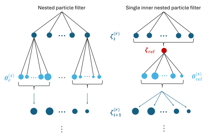
Figure 1: Visual explanation of the two variants of the nested particle filter for hierarchical Bayesian inference. Nested particle filter (left): For each particle $\zeta^{(r)}_{i}$ in the current outer ensemble (dark blue, top), a corresponding inner particle ensemble $\theta_{r}^{(1:S)}$ is initialized and weights $w_{r}^{(1:S)}$ are derived based on the observation model (light blue, area corresponds to weight), cf. (10). Subsequently, for each outer particle $\zeta^{(r)}_{i}$, its weight $v_{i}^{(r)}$ is updated based on $w_{r}^{(1:S)}$ (dark blue, bottom), cf. (12). In contrast, the single inner nested particle filter (right) generates a particle representation $\zeta_{\text{ref}}$ (red), which initializes only one reference inner particle ensemble $\theta_{\text{ref}}^{(1:S)}$. All outer weights $v_{i}^{(1:R)}$ are then updated simultaneously using the reference inner weights $w_{\text{ref}}^{(1:S)}$ adjusted to each outer particle by the individual importance ratio (13).

Input: Prior distribution $p$ for $\zeta$, data for all individuals $\mathbf{y}_{1:N}$, outer particle ensemble size $R$, inner particle ensemble size $S$, outer particle summary function

Output: Weighted outer particle ensemble $(v^{(1)}_{N},\zeta^{(1)}_{N}),...,(v^{(R)}_{N},\zeta^{(R)}_{N})$ such that $\sum_{r=1}^{R}v^{(r)}_{N}\delta_{\zeta^{(r)}_{N}}\approx p(\cdot|\mathbf{y}_{1:N})$

Initialization ($i=0$)

    Sample initial outer particle ensemble $\zeta^{(1:R)}_{0}$ from the prior $p$;

    Set $v^{(r)}_{0}=\frac{1}{R}$ for all $r$;

   

end

Sequential update ($i\mapsto i+1$)

    Input: Weighted outer particle ensemble $(v^{(1)}_{i},\zeta^{(1)}_{i}),...,(v^{(R)}_{i},\zeta^{(R)}_{i})$ such that $\sum_{r=1}^{R}v^{(r)}_{i}\delta_{\zeta^{(r)}_{i}}\approx p(\cdot|\mathbf{y}_{1:i})$, data for a new individual $\mathbf{y}_{i+1}$

    Output: Weighted outer particle ensemble $(v^{(1)}_{i+1},\zeta^{(1)}_{i+1}),...,(v^{(R)}_{i+1},\zeta^{(R)}_{i+1})$ such that $\sum_{r=1}^{R}v^{(r)}_{i+1}\delta_{\zeta^{(r)}_{i+1}}\approx p(\cdot|\mathbf{y}_{1:(i+1)})$

    Generate representation of outer ensemble: $\zeta_{\text{ref}}=\text{summary}\big{(}\zeta_{i}^{(1:R)},v_{i}^{(1:R)}\big{)}$;

    Sample a corresponding inner ensemble $\theta_{\text{ref}}^{(1:S)}\sim_{\text{iid}}p(\cdot|\zeta_{\text{ref}})$;

    for $s=1$ to $S$ do

       Calculate inner weights $w_{\text{ref}}^{(s)}=p(\mathbf{y}_{i+1}|\theta_{\text{ref}}^{(s)})$;

      

    end for

   for $r=1$ to $R$ do

       Update outer weights $v^{(r)}_{i+1}\propto v^{(r)}_{i}\cdot\sum_{s=1}^{S}\left(w_{\text{ref}}^{(s)}\cdot\frac{p(\theta_{\text{ref}}^{(s)}|\zeta^{(r)})}{p(\theta_{\text{ref}}^{(s)}|\zeta_{\text{ref}})}\right)$

    end for

   if $S_{\text{eff}}\,(v^{(1:R)}_{i+1})\geq\text{threshold}$ then

       $\zeta^{(r)}_{i+1}=\zeta^{(r)}_{i}$ for all $r$;

      

   else  // (Outer) resampling & rejuvenation

       $\zeta^{(1)}_{i+1},\ldots,\zeta^{(R)}_{i+1}\sim_{\text{iid}}\sum_{r=1}^{R}v^{(r)}_{i+1}\delta_{\zeta^{(r)}_{i}}$;

       $v^{(r)}_{i+1}=\frac{1}{R}$ for all $r$;

      

    end if

   

end

Algorithm 3 Single inner nested particle filter (sequential)

Parametric approximation + Metropolis-within-Gibbs sampling

All approaches described so far represent the marginal posterior $p(\zeta|\mathbf{y}_{1:N})$ nonparametrically (via a sample/particle ensemble). As an alternative, it can be approximated by a parametric class $p(\cdot\;;H)$, $H\in\mathbb{H}$, which we assume to be able to sample from. A special sequential algorithm can be designed if this class is conjugate to the distribution of the individual parameters $\theta$, i.e., for $\zeta\sim p(\cdot\;;H)$ there exists $H^{\prime}=H^{\prime}(\theta)\in\mathbb{H}$ such that $[\zeta|\theta]\sim p(\cdot\;;H^{\prime})$. In this case, a Metropolis-within-Gibbs algorithm can be used in every iteration to sample from $p(\zeta|\mathbf{y}_{1:i})$, coupled with a parametric approximation of $p(\zeta|\mathbf{y}_{1:i})$ based on the generated sample.

Gibbs sampling alternates between sampling from conditional distributions to sample from a joint distribution [10, 9], which is beneficial if sampling from conditional distributions is a structurally simpler problem. In Metropolis-within-Gibbs [11], direct sampling from some of these conditional distributions is replaced by Metropolis-Hastings sampling. In order to apply Gibbs sampling to the the marginal posterior $p(\zeta|\mathbf{y}_{1:(i+1)})$, the problem is augmented into a joint sampling problem from $p(\zeta,\theta_{i+1}|\mathbf{y}_{1:(i+1)})$; the $\theta_{i+1}$ component from the generated sample can then be simply ignored. The conditional distributions to sample from are $p(\zeta^{(l)}|\theta^{(l-1)}_{i+1},\mathbf{y}_{1:(i+1)})$ and $p(\theta^{(l)}_{i+1}|\zeta^{(l)},\mathbf{y}_{1:(i+1)})$, coupled by the iterative update of each other.

As a preparation to Gibbs sampling, and similarly to the single inner nested particle filter, a single ensemble $\theta_{\text{ref}}^{(1)},...,\theta_{\text{ref}}^{(S)}$ is first sampled from $p(\cdot|\zeta_{\text{ref}})$ with a suitably chosen reference value $\zeta_{\text{ref}}$, derived as a summary of $p(\cdot;H_{i})$, e.g. $\zeta_{\text{ref}}=\mathbb{E}_{H_{i}}[\zeta]$. Subsequently, a weighted ensemble $(w_{\text{ref}}^{(s)},\theta_{\text{ref}}^{(s)})$, $s\in\{1,...,S\}$, is determined (non-hierarchical particle filter); $\sum_{s=1}^{S}w_{\text{ref}}^{(s)}\delta_{\theta_{\text{ref}}^{(s)}}$ is then an approximation of $p(\,\cdot\,|\zeta_{\text{ref}},\mathbf{y}_{i+1})$.

Gibbs sampling is then performed as follows:

• Direct sampling $\zeta^{(l)}\sim p(\cdot\,|\theta_{i+1}^{(l-1)},\mathbf{y}_{1:(i+1)})$:

  • By the parametric approximation from the previous step, $p(\zeta|\mathbf{y}_{1:i})=p(\zeta;H_{i})$ for some $H_{i}\in\mathbb{H}$;

  • Using the sequential Bayes’ formula (11), but conditioned on the individual parameters $\theta_{i+1}$,

    $$p(\zeta|\theta_{i+1},\mathbf{y}_{1:(i+1)})\propto p(\mathbf{y}_{i+1}|\theta_{i+1},\zeta)\cdot p(\zeta|\theta_{i+1},\mathbf{y}_{1:i});$$

  • By conditional independence, $p(\mathbf{y}_{i+1}|\theta_{i+1},\zeta)=p(\mathbf{y}_{i+1}|\theta_{i+1})$ and hence, this term cancels due to normalization, which yields

    $$p(\zeta|\theta_{i+1},\mathbf{y}_{1:(i+1)})\propto p(\zeta|\theta_{i+1},\mathbf{y}_{1:i});$$

  • Due to the conjugacy assumption, $p(\zeta|\theta_{i+1},\mathbf{y}_{1:i})=p(\zeta;H^{\prime})$ for some $H^{\prime}=H^{\prime}(\theta_{i+1})$, which can be sampled from.

• Metropolis-Hastings sampling $\theta_{i+1}^{(l)}\sim p(\cdot\,|\zeta^{(l)},\mathbf{y}_{1:(i+1)})$:

  • By conditional independence, $p(\theta_{i+1}|\zeta,\mathbf{y}_{1:(i+1)})=p(\theta_{i+1}|\zeta,\mathbf{y}_{i+1})$ (also note that it is not a marginal posterior);

  • A proposal $\theta_{i+1}^{*}\sim\sum_{s=1}^{S}w_{\text{ref}}^{(s)}\delta_{\theta_{\text{ref}}^{(s)}}$ is drawn and rejuvenated, constituting an approximate sample from $p(\cdot|\zeta_{\text{ref}},\mathbf{y}_{i+1})$ (independence sampling);

  • The acceptance probability for $\theta_{i+1}^{*}$ (see also Eq. (7)) is then given by

    $$\frac{p(\theta_{i+1}^{\ast}|\zeta^{(l)},\mathbf{y}_{i+1})}{p(\theta_{i+1}^{(l-1)}|\zeta^{(l)},\mathbf{y}_{i+1})}\cdot\frac{p(\theta_{i+1}^{(l-1)}|\zeta_{\text{ref}},\mathbf{y}_{i+1})}{p(\theta_{i+1}^{\ast}|\zeta_{\text{ref}},\mathbf{y}_{i+1})}$$

    $$=\frac{p(\mathbf{y}_{i+1}|\theta_{i+1}^{\ast})p(\theta_{i+1}^{\ast}|\zeta^{(l)})}{p(\mathbf{y}_{i+1}|\theta_{i+1}^{(l-1)})p(\theta_{i+1}^{(l-1)}|\zeta^{(l)})}\cdot\frac{p(\mathbf{y}_{i+1}|\theta_{i+1}^{(l-1)})p(\theta_{i+1}^{(l-1)}|\zeta_{\text{ref}})}{p(\mathbf{y}_{i+1}|\theta_{i+1}^{\ast})p(\theta_{i+1}^{\ast}|\zeta_{\text{ref}})}$$

    $$=\frac{p(\theta_{i+1}^{\ast}|\zeta^{(l)})}{p(\theta_{i+1}^{(l-1)}|\zeta^{(l)})}\cdot\frac{p(\theta_{i+1}^{(l-1)}|\zeta_{\text{ref}})}{p(\theta_{i+1}^{\ast}|\zeta_{\text{ref}})}$$

    The advantage of this formulation is that the observation model (3) need not be evaluated during Gibbs sampling (the resulting expression is independent of $\mathbf{y}_{i+1}$).

The detailed steps for this algorithm are given in Algorithm 4.

Input: Data for all individuals $\mathbf{y}_{1:N}$, parametrized prior distribution $p(\zeta)=p(\zeta;H_{0})$, inner ensemble size $S$, length of Markov chain $L$, summary function for $p(\cdot;H)$, estimator for $H$ from observed samples $\zeta^{(1:L)}$

Output: Hyperparameter $H_{N}$ of the parametric approximation $p(\zeta;H_{N})$ to the posterior $p(\zeta|\mathbf{y}_{1:N})$.

Requirement : Conjugacy of $p(\cdot;H)$ to $p(\theta|\zeta)$, i.e., for each $H\in\mathbb{H}$ there is a $H^{\prime}\in\mathbb{H}$ such that $p(\zeta;H^{\prime})\propto p(\theta|\zeta)p(\zeta;H)$

Sequential update ($i\mapsto i+1$)

    Input: Hyperparameter $H_{i}$, data for a new individual $\mathbf{y}_{i+1}$

    Output: Updated hyperparameter $H_{i+1}$

    Generate representation of parametric distribution: $\zeta_{\text{ref}}=\text{summary}\big{(}p(\,\cdot\,;H_{i})\big{)}$;

    Sample a corresponding inner ensemble $\theta_{\text{ref}}^{(1:S)}\sim_{\text{iid}}p(\cdot\,|\zeta_{\text{ref}})$;

    for $s=1$ to $S$ do

       Calculate inner weights $w_{\text{ref}}^{(s)}=p(\mathbf{y}_{i+1}|\theta_{\text{ref}}^{(s)})$ ;

        // Possibly resampling & rejuvenation

      

    end for

   Gibbs sampling:

   [3mm] for $l=1$ to $L$ do

       Direct sampling: $\zeta^{(l)}\sim p(\cdot\,|\theta_{i+1}^{(l-1)})$ ;

        // Requirement is used here

       Metropolis-Hastings sampling: $\theta_{i+1}^{\ast}\sim\sum_{s=1}^{S}w_{\text{ref}}^{(s)}\delta_{\theta_{\text{ref}}^{(s)}}$ plus rejuvenation, then with probability

$$\alpha=\min\left(1,\,\frac{p(\theta_{i+1}^{\ast}|\zeta^{(l)})}{p(\theta_{i+1}^{(l-1)}|\zeta^{(l)})}\cdot\frac{p(\theta_{i+1}^{(l-1)}|\zeta_{\text{ref}})}{p(\theta_{i+1}^{\ast}|\zeta_{\text{ref}})}\right)$$

set $\theta_{i+1}^{(l)}=\theta_{i+1}^{\ast}$, otherwise $\theta_{i+1}^{(l)}=\theta_{i+1}^{(l-1)}$;

      

    end for

   Parametric approximation of posterior:

   [3mm] estimate $H_{i+1}$ based on $\zeta^{(1:L)}$ such that $p(\cdot\,;H_{i+1})\approx\sum_{l=1}^{L}\delta_{\zeta^{(l)}}$

end

Algorithm 4 Parametric approximation + Metropolis-within-Gibbs sampling (sequential)

3 Numerical experiments

Pharmacokinetic model

As an example model to evaluate the different algorithms, we considered a one-compartment pharmacokinetic model, with a single intravenous bolus dose $d=100\,\mu\text{mol}$ administered at time 0 and first order elimination kinetics. In this model, the plasma concentration $C(t,\theta)$ predicted at time $t$ can be computed analytically:

$$C(t,\theta)=\frac{D}{V}\exp\left(-\frac{e^{\theta}t}{V}\right),$$ (14)

with volume of distribution $V$ and log-clearance $\theta$. While $V=20$ L is assumed to be fixed, inter-individual variability (IIV) is assumed on log-clearance, given by a normal distribution (corresponding to a lognormally distributed clearance)

$$\theta_{i}\sim\mathcal{N}(\mu_{\text{CL}},\omega^{2}_{\text{CL}}).$$ (15)

Additionally, we assume random unexplained variability (RUV) on the observed data, given by an additive error on log-scale:

$$[y_{ij}|\theta_{i}]\sim\log\mathcal{N}\Big{(}\log\big{(}C(t_{ij},\theta_{i})\big{)},\sigma^{2}\Big{)},$$ (16)

with error variance (on log scale) $\sigma^{2}$. That is, $\zeta=(\mu_{\text{CL}},\omega^{2}_{\text{CL}})$, with $V$, $\sigma^{2}$ being assumed to be known from the prior data.

Prior distribution

As a prior for the population parameters $\mu_{\text{CL}},\omega^{2}_{\text{CL}}$, a normal-inverse gamma distribution

$$(\mu_{CL},\omega^{2}_{CL})\sim\text{N-}\Gamma^{-1}(\mu_{0},\kappa_{0},\alpha_{0},\beta_{0})$$ (17)

is chosen, with parameters $\mu_{0}=\log(5)$, $\kappa_{0}=1$, $\alpha_{0}=10$ and $\beta_{0}=2.7$. This distribution is conjugate to a normal distribution with unknown mean and variance, a necessary requirement to use Algorithm 4 (parametric approximation + Metropolis-within-Gibbs). Of note, this specific choice is not required for any of the other algorithms.

Data generation

We considered a simulation study in order to have a scenario in which the ground truth is known and where algorithms can be compared. Mimicking the anticipated change of distribution between trial and real-world data, individual parameters $\theta_{1},...,\theta_{N}$ were assumed to originate from a distribution that is very unlikely under the prior, namely a normal distribution with parameters

$$\zeta_{\text{true}}=(\mu_{\text{CL,true}},\omega^{2}_{\text{CL,true}})=(\log(2),0.1),$$

which corresponds to a median clearance of 2 L/h. Four scenarios of different data sparsity were considered, with either $n=20$ or $n=100$ individuals, and per individual either a sparse sampling scheme with observation times $t=$ 0 h and 1 h, or a rich sampling scheme with observation times $t=$ 0 h, 1 h, 2 h, 5 h, 11 h, 23 h and 47 h.

Algorithmic considerations

For the pseudo-marginal Metropolis-Hastings algorithm, $M=25$ Monte Carlo samples were used in (8), and a chain length of $L=10^{4}$ (with 10% burn-in). Based on preliminary testing, the proposal distribution

$$q(\zeta^{*}|\zeta)=\mathcal{N}\left(\zeta,\begin{pmatrix}0.2&0\\ 0&0.2\end{pmatrix}\right)$$

was chosen.

For the nested and single inner nested particle filters, $S=R=1000$ outer and inner particles were used. For the single inner nested particle filter, the outer ensemble was summarized via the componentwise weighted median (i.e., the median of the empirical distribution $\sum_{r=1}^{R}v_{r}^{i}\delta_{\zeta_{r}^{i}}$ of the posterior approximation). No rejuvenation was used for either particle filter method (see also Sec. 4).

For the parametric approximation + Metropolis-within-Gibbs algorithm, a normal-inverse gamma distribution was assumed (a special case of the normal-inverse Wishart distribution for the multivariate case), which is conjugate to a normal distribution with unknown mean and variance, cf. (15) and (17). The representation $\zeta_{\text{ref}}$ was chosen to be the mean of the parametric distribution $p(\cdot\,;H_{i})$. As for pseudo-marginal Metropolis-Hastings, a chain length of $L=10^{4}$ with 10% burn-in was used. The parameter $H_{i+1}$ from the parametric approximation was estimated from the sample $\zeta^{(1:L)}$ resulting from the Metropolis-within-Gibbs procedure by matching theoretical and empirical mean and variance. For the rejuvenation step, a normal distribution with standard deviation of 0.1% of the sampled individual parameter $\theta_{i+1}^{*}$ was chosen.

Results

For each data scenario, we simulated a real-world population of individuals and investigated all algorithms for hierarchical Bayesian inference. The results are shown in Figure 2. As expected, the reference method (pseudo-marginal Metropolis-Hastings with importance sampling) covers the data-generating parameters in all data sparsity scenarios, with more uncertainty under more sparse conditions. The two particle filters (nested and single inner nested particle filter) show a very similar behaviour to each other, consistent with the reference method in rich data scenarios, but overconfident in more sparse data scenarios. Finally, the parametric approximation + Metropolis-within-Gibbs algorithm is only accurate in the data-richest scenario, while it is overconfident and even biased in more sparse scenarios.

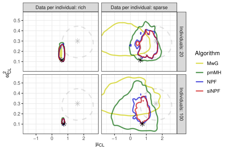
Figure 2: Accuracy comparison of different algorithm for marginal posterior inference. The prior distribution $p(\zeta)$ is shown in grey dashed line, with its mean indicated by the grey star. Colored bold lines represent different approximations to the marginal posterior $p(\zeta|\mathbf{y}_{1:N})$. All distributions are represented as 80% highest density regions based on kernel density estimation. The data-generating parameters $\zeta_{\text{true}}$ are shown as a black star.
Abbreviations: MwG = Metropolis-within-Gibbs & parametric approximation; pmMH = pseudo-marginal Metropolis-Hastings with importance sampling; NPF = nested particle filter; siNPF = single inner nested particle filter.

Runtimes were compared between the four algorithms for a single batch inference on all individuals (see Table 1). Compared to the reference method (pseudo-marginal Metropolis-Hastings with importance sampling), the nested particle filter took slightly (approx. 25%) longer, while the parametric approximation + Metropolis-within-Gibbs and single inner nested particle filter were 20 times and 300 times faster, respectively. Runtimes in different data sparsity scenarios were almost unaffected by the number of datapoints used per individual and scaled linearly with the number of individuals. Therefore, the above relative runtime comparisons were independent of the data sparsity scenario. Comparing the nested and single inner nested particle filters, a 400 fold speedup was observed by avoiding the creation of 1000$\times$1000 inner particles. For more costly models, this accelaration factor is expected to increase roughly to the number of outer particles (here, 1000). Of note, in a setting where forecasting after each individual is required, the runtime cost for batch algorithms would increase considerably, by a factor roughly proportional to the number of individuals considered.

	$N=20$		$N=100$
Algorithm	sparse	rich	sparse	rich
pseudo-marginal Metropolis-Hastings	1268 s	1190 s	5581 s	–
nested particle filter	1590 s	1635 s	7904 s	8183 s
single inner nested particle filter	4 s	4 s	20 s	21 s
parametric approximation	82 s	84 s	422 s	419 s

Table 1: Runtime comparison of the different algorithms (MacBook Pro, 2 GHz Quad-Core Intel Core i5 processor, 16 GB 3733 MHz LPDDR4X memory).

4 Conclusion

In this work, we evaluated the accuracy and runtime of different algorithms for hierarchical Bayesian estimation in a simplified MIPD setting. The pseudo-marginal Metropolis-Hastings algorithm was considered as a reference method, and it showed consistent behaviour in all scenarios. Three sequential algorithms were considered, a previously investigated parametric approximation + Metropolis-within-Gibbs and two variants of nested particle filters. Consistent with [15], we observed that the parametric approximation + Metropolis-within-Gibbs algorithm yielded incorrect posterior distribution estimates in sparse data scenarios. A possible reason could be the sequential amplification of approximation errors of the posterior within the parametric class. The nested particle filters showed better accuracy, but still slight overconfidence in the posterior. Compared to the nested particle filter, the single inner nested particle filter resulted in very similar performance at greatly reduced runtime; overall, it had a good tradeoff between accuracy and computational cost. For sampling a reference ensemble, the median was used to summarize the population distribution, which worked well in the simple model considered here. In more complex (and higher-dimensional) models, a variance inflated summary might be appropriate to achieve a better parameter space coverage. Furthermore, the remaining misfit of particle filters might be addressed by appropriately chosen particle rejuvenation. Future work will further develop these algorithms in order to carry over rejuvenated particles from the inner to the outer level. Finally, more complex PK models will be studied in future work, in particular the neutropenia setting investigated in [15].

Funding note

The research has been funded by the Deutsche Forschungsgemeinschaft (DFG) – Project-ID 318763901 – SFB1294.

References

- [1] Christophe Andrieu and Gareth O. Roberts. The pseudo-marginal approach for efficient Monte Carlo computations. The Annals of Statistics, 37(2), April 2009.
- [2] M.S. Arulampalam, S. Maskell, N. Gordon, and T. Clapp. A tutorial on particle filters for online nonlinear/non-Gaussian Bayesian tracking. IEEE Transactions on Signal Processing, 50(2):174–188, 2002.
- [3] Mark A Beaumont. Estimation of Population Growth or Decline in Genetically Monitored Populations. Genetics, 164(3):1139–1160, July 2003.
- [4] N. Chopin, P. E. Jacob, and O. Papaspiliopoulos. SMC2: An Efficient Algorithm for Sequential Analysis of State Space Models. Journal of the Royal Statistical Society Series B: Statistical Methodology, 75(3):397–426, October 2012.
- [5] Emmanuelle Comets, Audrey Lavenu, and Marc Lavielle. Parameter Estimation in Nonlinear Mixed Effect Models Using saemix, an R Implementation of the SAEM Algorithm. Journal of Statistical Software, 80(3), 2017.
- [6] Dan Crisan and Joaquín Míguez. Nested particle filters for online parameter estimation in discrete-time state-space Markov models. Bernoulli, 24(4A), November 2018.
- [7] Bernard Delyon, Marc Lavielle, and Eric Moulines. Convergence of a stochastic approximation version of the EM algorithm. The Annals of Statistics, 27(1), March 1999.
- [8] Jos Elfring, Elena Torta, and René van de Molengraft. Particle Filters: A Hands-On Tutorial. Sensors, 21(2):438, January 2021.
- [9] Alan E. Gelfand and Adrian F. M. Smith. Sampling-Based Approaches to Calculating Marginal Densities. Journal of the American Statistical Association, 85(410):398–409, June 1990.
- [10] Stuart Geman and Donald Geman. Stochastic Relaxation, Gibbs Distributions, and the Bayesian Restoration of Images. IEEE Transactions on Pattern Analysis and Machine Intelligence, PAMI-6(6):721–741, November 1984.
- [11] W. R. Gilks, N. G. Best, and K. K. C. Tan. Adaptive Rejection Metropolis Sampling within Gibbs Sampling. Applied Statistics, 44(4):455, 1995.
- [12] W. K. Hastings. Monte Carlo sampling methods using Markov chains and their applications. Biometrika, 57(1):97–109, April 1970.
- [13] Ron J. Keizer, Rob ter Heine, Adam Frymoyer, Lawrence J. Lesko, Ranvir Mangat, and Srijib Goswami. Model‐Informed Precision Dosing at the Bedside: Scientific Challenges and Opportunities. CPT: Pharmacometrics & Systems Pharmacology, 7(12):785–787, October 2018.
- [14] Franziska Kluwe, Robin Michelet, Anna Mueller‐Schoell, Corinna Maier, Lena Klopp‐Schulze, Madelé van Dyk, Gerd Mikus, Wilhelm Huisinga, and Charlotte Kloft. Perspectives on Model‐Informed Precision Dosing in the Digital Health Era: Challenges, Opportunities, and Recommendations. Clinical Pharmacology & Therapeutics, 109(1):29–36, October 2020.
- [15] Corinna Maier, Jana de Wiljes, Niklas Hartung, Charlotte Kloft, and Wilhelm Huisinga. A continued learning approach for model‐informed precision dosing: Updating models in clinical practice. CPT: Pharmacometrics & Systems Pharmacology, 11(2):185–198, December 2021.
- [16] Corinna Maier, Niklas Hartung, Jana de Wiljes, Charlotte Kloft, and Wilhelm Huisinga. Bayesian Data Assimilation to Support Informed Decision Making in Individualized Chemotherapy. CPT: Pharmacometrics & Systems Pharmacology, 9(3):153–164, January 2020.
- [17] Nicholas Metropolis, Arianna W. Rosenbluth, Marshall N. Rosenbluth, Augusta H. Teller, and Edward Teller. Equation of State Calculations by Fast Computing Machines. The Journal of Chemical Physics, 21(6):1087–1092, June 1953.
- [18] Richard W. Peck. Precision Dosing: An Industry Perspective. Clinical Pharmacology & Therapeutics, 109(1):47–50, October 2020.
- [19] Lewis B. Sheiner and Stuart L. Beal. Evaluation of methods for estimating population pharmacokinetic parameters. I. Michaelis-Menten model: Routine clinical pharmacokinetic data. Journal of Pharmacokinetics and Biopharmaceutics, 8(6):553–571, December 1980.
- [20] Liyuan Wang, Xingxing Zhang, Hang Su, and Jun Zhu. A Comprehensive Survey of Continual Learning: Theory, Method and Application. IEEE Transactions on Pattern Analysis and Machine Intelligence, 46(8):5362–5383, August 2024.