Variational Deep Learning via Implicit Regularization

Abstract

Modern deep learning models generalize remarkably well in-distribution, despite being overparametrized and trained with little to no explicit regularization. Instead, current theory credits implicit regularization imposed by the choice of architecture, hyperparameters and optimization procedure. However, deploying deep learning models out-of-distribution, in sequential decision-making tasks, or in safety-critical domains, necessitates reliable uncertainty quantification, not just a point estimate. The machinery of modern approximate inference — Bayesian deep learning — should answer the need for uncertainty quantification, but its effectiveness has been challenged by our inability to define useful explicit inductive biases through priors, as well as the associated computational burden. Instead, in this work we demonstrate, both theoretically and empirically, how to regularize a variational deep network implicitly via the optimization procedure, just as for standard deep learning. We fully characterize the inductive bias of (stochastic) gradient descent in the case of an overparametrized linear model as generalized variational inference and demonstrate the importance of the choice of parametrization. Finally, we show empirically that our approach achieves strong in- and out-of-distribution performance without tuning of additional hyperparameters and with minimal time and memory overhead over standard deep learning.

1 Introduction

The success of deep learning across many application domains is, on the surface, remarkable, given that deep neural networks are usually overparameterized and trained with little to no explicit regularization. The generalization properties observed in practice have been explained by implicit regularization instead, resulting from the choice of architecture [1], hyperparameters [2, 3], and optimizer [4, 5, 6, 7, 8, 9, 10]. Notably, the corresponding inductive biases often require no additional computation, in contrast to enforcing a desired inductive bias through explicit regularization.

In the last two decades, there has been an increasing focus on improving the reliability and robustness of deep learning models via (approximately) Bayesian approaches [11] to improve performance on out-of-distribution data [12], in continual learning [13] and sequential decision-making [14]. However, despite its promise, in practice, Bayesian deep learning can suffer from issues with prior elicitation [15], can be challenging to scale [16], and explicit regularization from the prior combined with approximate inference may result in pathological inductive biases and uncertainty [17, 18, 19, 20].

In this work, we demonstrate both theoretically and empirically how to exploit the implicit bias of optimization for approximate inference in probabilistic neural networks, thus regularizing training implicitly rather than explicitly via the prior. This not only narrows the gap to how standard neural networks are trained, but also reduces the computational overhead of training compared to variational inference. More specifically, we propose to learn a variational distribution over the weights of a deep neural network by maximizing the expected log-likelihood in analogy to training via maximum likelihood in the standard case. However, in contrast to variational Bayes, there is no explicit regularization via a Kullback-Leibler divergence to the prior. Surprisingly, we show theoretically and empirically that training this way does not cause uncertainty to collapse away from the training data, if initialized and parametrized correctly. More so, for overparametrized linear models we rigorously characterize the implicit bias of SGD as generalized variational inference with a 2-Wasserstein regularizer penalizing deviations from the prior. Figure 1 illustrates our approach on a toy example.

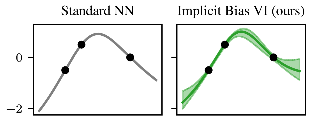
(a) Implicit regularization.

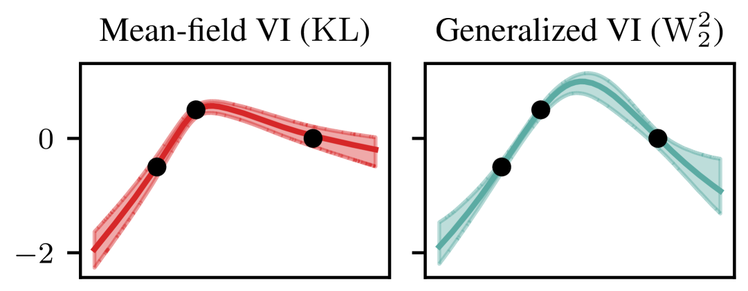
(b) Explicit regularization.

Figure 1: Variational deep learning via implicit regularization. Neural networks generalize well without explicit regularization due to implicit regularization from the architecture and optimization. We can exploit this implicit bias for variational deep learning, removing the computational overhead of explicit regularization and narrowing the gap to deep learning practice. As illustrated for a two-hidden layer MLP and proven rigorously for overparametrized linear models in Theorems 1 and 2, the implicit bias of (S)GD in variational networks (see 1(a)) can be understood as generalized variational inference with a 2-Wasserstein regularizer (see 1(b)). This differs from the standard ELBO objective with a KL divergence to the prior as used for example in mean-field VI (see 1(b)).

Contributions

In this work, we propose a new approach to uncertainty quantification in deep learning that exploits the implicit regularization of (stochastic) gradient descent. We precisely characterize this implicit bias for regression (Theorem 1) and binary classification (Theorem 2) in overparameterized linear models, generalizing results for non-probabilistic models and drawing a rigorous connection to generalized Bayesian inference. We also demonstrate the importance of the parametrization for the inductive bias and its impact on hyperparameter choice. Finally, in several benchmarks we demonstrate competitive performance to state-of-the-art baselines for Bayesian deep learning, at minimal computational overhead compared to standard neural networks.

2 Background

Given a training dataset $({\bm{X}},{\bm{y}})=\{({\bm{x}}_{n},y_{n})\}_{n=1}^{N}$ of input-output pairs, supervised learning seeks a model $f_{\bm{w}}({\bm{x}})$ to predict the corresponding output $y({\bm{x}})$ for a test input ${\bm{x}}$. The parameters ${\bm{w}}\in\mathbb{R}^{P}$ of the model are typically trained via empirical risk minimization, i.e.

$${\bm{w}}_{\star}\in\operatorname*{arg\,min}_{\bm{w}}\ell_{R}({\bm{w}})\qquad\textrm{with}\qquad\ell_{R}({\bm{w}})=\ell({\bm{y}},f_{\bm{w}}({\bm{X}}))+\lambda R({\bm{w}}),$$ (1)

where the loss $\ell({\bm{y}},f_{\bm{w}}({\bm{X}}))$ encourages fitting the training data and the regularizer $R({\bm{w}})$, given some $\lambda>0$, discourages overfitting, which can lead to poor generalization on test data.

Implicit Bias of Optimization One of the remarkable observations in deep learning is that training overparametrized models ($P>N$) with gradient descent without explicit regularization can nonetheless lead to good generalization [21] because the optimizer, initialization, and parametrization implicitly regularize the optimization problem $\operatorname*{arg\,min}_{\bm{w}}\ell({\bm{y}},f_{\bm{w}}({\bm{X}}))$ [[, e.g. ]]Soudry2018ImplicitBias,Gunasekar2018CharacterizingImplicit,Nacson2019StochasticGradient,Vardi2023ImplicitBias,Vasudeva2024ImplicitBias.

Variational Inference Bayesian inference quantifies uncertainty in the parameters, and consequently predictions, by the posterior distribution $p({\bm{w}}\mid{\bm{X}},{\bm{y}})\propto p({\bm{y}}\mid{\bm{X}},{\bm{w}})p({\bm{w}})$, which depends on the choice of a prior belief $p({\bm{w}})$ and a likelihood $p(y\mid{\bm{w}})$. Approximating the posterior with $q_{{\bm{\theta}}}\approx p({\bm{w}}\mid{\bm{X}},{\bm{y}})$ by maximizing a lower bound to the log-evidence leads to the following variational optimization problem [24]:

$${\bm{\theta}}_{\star}\in\operatorname*{arg\,min}_{{\bm{\theta}}}\ell_{R}({\bm{\theta}})\qquad\textrm{with}\qquad\ell_{R}({\bm{\theta}})=\operatorname{\mathbb{E}}_{q_{{\bm{\theta}}}({\bm{w}})}\mathopen{}\left(-\log p({\bm{y}}\mid{\bm{w}})\right)+\operatorname{KL}\mathopen{}\left(q_{{\bm{\theta}}}({\bm{w}})\;\middle\|\;p({\bm{w}})\right).$$ (2)

Equation 2 is an instance of the optimization problem in Equation 1 where the optimization is over the variational parameters ${\bm{\theta}}$ of the posterior approximation $q_{{\bm{\theta}}}({\bm{w}})$. In the case of a potentially misspecified prior or likelihood, the variational formulation (2) can be generalized to arbitrary loss functions $\ell$ and statistical distances $\operatorname{D}$ to the prior [25, 26, 27], such that

$$\ell_{R}({\bm{\theta}})=\operatorname{\mathbb{E}}_{q_{{\bm{\theta}}}({\bm{w}})}\mathopen{}\left(\ell({\bm{y}},f_{\bm{w}}({\bm{X}}))\right)+\lambda\operatorname{D}(q_{{\bm{\theta}}},p).$$ (3)

3 Variational Deep Learning via Implicit Regularization

Our goal is to learn a variational distribution $q_{\bm{\theta}}({\bm{w}})$ for the parameters ${\bm{w}}$ of a neural network, as in a Bayesian neural network. However, in contrast to training with (generalized) variational inference, which has an explicit regularization term defined via the prior to avoid overfitting, we will demonstrate how to perform variational inference over the weights of a deep neural network purely via implicit regularization, removing the need to store and compute quantities involving the prior entirely. We will see that this approach inherits the well-established optimization toolkit from deep learning seamlessly, while providing uncertainty quantification at minimal overhead.

3.1 Training via the Expected Loss

Rather than performing variational inference by explicitly regularizing the variational distribution to remain close to the prior, we propose to train by minimizing the expected loss $\bar{\ell}({\bm{\theta}})$ in analogy to how deep neural networks are usually trained. Therefore, the optimal variational parameters are given by

$${\bm{\theta}}_{\star}\in\operatorname*{arg\,min}_{{\bm{\theta}}}\underbracket{\operatorname{\mathbb{E}}_{q_{{\bm{\theta}}}({\bm{w}})}\mathopen{}\left(\ell({\bm{y}},f_{\bm{w}}({\bm{X}}))\right)}_{\coloneqq\bar{\ell}({\bm{\theta}})}{\color[rgb]{.5,.5,.5}\,{\markoverwith{{\color[rgb]{0.83984375,0.15234375,0.15625}\rule[4.30554pt]{2.0pt}{0.8pt}}}\ULon{+\operatorname{D}(q_{{\bm{\theta}}},p)}}.\end{equation}Practically,thismeanswedonotneedtocomputetheregularizationtermanditsgradientduringtrainingandwedonotneedtoallocateadditionalmemoryforthepriorhyperparameters.However,atfirstglancemodifyingthevariationalobjectivein\lx@cref{creftype~refnum}{eqn:variational-objective}byremovingthedivergencetermseemstodefeatthepurposeofaBayesianapproachentirely.Wearecompletelyomittingthepriorfromthetrainingloss.Whyshouldtheuncertaintyovertheweightsnotcollapse?Howdoesthisincorporateanypriorinformation?\par}$$ (4)

3.2 Implicit Bias of (S)GD as Generalized Variational Inference

Unexpectedly, training via the expected loss achieves regularization to the prior solely by initializing (stochastic) gradient descent to the prior, as we will prove in Section 4 for an overparametrized linear model. Moreover, we can characterize this implicit regularization exactly. (S)GD converges to a global minimum ${\bm{\theta}}_{\star}^{\textnormal{GD}}\in\operatorname*{arg\,min}\bar{\ell}({\bm{\theta}})$ of the training loss, given an appropriate learning rate sequence. But among the global minima, if (S)GD is initialized to the parameters of the prior and the Gaussian variational family is parametrized appropriately, then the solution identified by (S)GD minimizes the 2-Wasserstein distance to the prior, i.e.

$$q_{{\bm{\theta}}_{\star}^{\textnormal{GD}}}=\operatorname*{arg\,min}_{\begin{subarray}{c}q_{\bm{\theta}}\\ \textrm{s.t.\@\ }{\bm{\theta}}\in\operatorname*{arg\,min}\bar{\ell}({\bm{\theta}})\end{subarray}}\operatorname{W}_{2}^{2}\mathopen{}\left(q_{{\bm{\theta}}},p\right).$$

This equation shows that the implicit bias of (S)GD is such that it converges to a generalized variational posterior, minimizing Eq. 3 for a certain regularization strength, but with a regularizer that is not a KL divergence as it would be for standard variational inference, but rather a 2-Wasserstein distance to the prior. Given this characterization, we call our method Implicit Bias VI.

Section 4 provides a detailed version of the regression results introduced here and proves a similar result for binary classification. Our experiments in Section 5 focus on the application to deep neural networks. Since training via the expected loss can achieve zero loss in overparameterized models, we expect our approach to mimic vanilla deep networks closely in-distribution, while falling back to the prior out-of-distribution, as enforced by the 2-Wasserstein regularizer.

3.3 Computational Efficiency

In practice, we minibatch the expected loss both over training data and parameter samples ${\bm{w}}_{m}$ drawn from the variational distribution $q_{\bm{\theta}}({\bm{w}})$ such that

$$\bar{\ell}({\bm{\theta}})=\operatorname{\mathbb{E}}_{q_{{\bm{\theta}}}({\bm{w}})}\mathopen{}\left(\ell({\bm{y}},f_{\bm{w}}({\bm{X}}))\right)\approx\frac{1}{N_{b}M}\sum_{n=1}^{N_{b}}\sum_{m=1}^{M}\ell({\bm{y}}_{n},f_{{\bm{w}}_{m}}({\bm{X}}_{n})).$$ (5)

The training cost is primarily determined by two factors. The number of parameter samples $M$ we draw for each evaluation of the objective, and the variational family, which determines the number of additional parameters of the model and the cost for sampling a set of parameters in each forward pass. We wish to keep the overhead compared to a vanilla deep neural network as small as possible.

Training With A Single Parameter Sample ($M=1$)

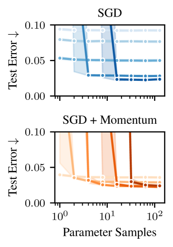
Figure 2: Training with a single parameter sample given a small enough learning rate. Lighter color shades correspond to smaller learning rates. See also Section S3.2.

When drawing fewer parameter samples ${\bm{w}}_{m}$ the training objective in Eq. 5 becomes noisier in the same way a smaller batch size impacts the loss. This is concerning since the optimization procedure may not converge given this additional noise. However, one can train with a single parameter sample only, simply by reducing the learning rate appropriately, as we show experimentally in Figure 2 and Section S3.2. Therefore given a set of sampled parameters, the cost of a forward and backward pass is identical to a standard neural network (up to the overhead of the covariance parameters). In analogy to the previously observed relationship [[, e.g.,]]Goyal2018AccurateLarge,Smith2018BayesianPerspective,Smith2018DontDecay between the optimal batch size $N_{b}$, learning rate $\eta$ and momentum $\gamma$, when optimizing the expected loss we conjecture the following scaling law for the optimal batch size $N_{b}$ and number of parameter samples $M$:

$$\textstyle N_{b}M\propto\frac{\eta}{1-\gamma}.$$ (6)

Figure 2 illustrates this. When using fewer parameter samples in the expected loss, training is unstable unless the learning rate is chosen sufficiently small. For a fixed number of optimizer steps this decreases performance, but either training for more steps, or using momentum closes this gap. As predicted by Eq. 6, momentum requires a smaller learning rate than vanilla SGD.

Variational Family and Covariance Structure

We choose a Gaussian variational distribution $q_{\bm{\theta}}({\bm{w}})$ over (a subset of the) weights of the neural network. While at first glance this may seem restrictive, there is ample evidence that variational families in deep neural networks do not need to be complex to be expressive [31, 32]. In fact, in analogy to deep feedforward NNs with ReLU activations being universal approximators [33], one can show that Bayesian neural networks with ReLU activations and at least one Gaussian hidden layer are universal conditional distribution approximators, meaning they can approximate any continuous conditional distribution arbitrarily well [32]. As we show in Section 4, training an overparametrized linear model with SGD via the expected loss amounts to generalized variational inference if the covariance is factorized, i.e. ${\bm{\Sigma}}={\bm{S}}{\bm{S}}^{\mathsf{T}}$ where ${\bm{S}}\in\mathbb{R}^{P\times R}$ is a dense matrix with rank $R\leq P$. Note that this (low-rank) parametrization of a covariance is non-standard in the sense that the implicit regularization result does not hold in the same form for a Cholesky factorization! Motivated by the theoretical observation of the implicit bias in Theorem 1, we use Gaussian layers with factorized covariances for all architectures.

3.4 Parametrization, Feature Learning and Hyperparameter Transfer

The inductive bias of SGD in the variational setting is determined by the initialization and variational parametrization, as we’ve seen above, and is formalized in Theorem 1. What is not covered, but not unusual in practice, are layer-specific learning rates. Luckily, these can be absorbed into the weights of the model and the initialization, resulting in a single global learning rate [[, Lemma J.1,]]Yang2021TensorProgramsa. We refer to this set of choices — initialization, (variational) parameters and layer-specific learning rates — as the parametrization of a variational neural network in analogy to how the term is used in deep learning. While parameterization is well-studied for non-probabilistic deep learning, it has been identified as one of the “grand challenges of Bayesian computation” [35].

The “standard parameterization” (SP) initializes the weights of a neural network randomly from a distribution with variance $\propto 1/\texttt{fan\_in}$ (e.g., as in Kaiming initialization, the PyTorch default) and makes no further adjustments to the forward pass or learning rate. In contrast, the maximal update parametrization ($\mu$P) [36] ensures feature learning even as the width of the network tends to infinity. Feature learning is at the core of the modern deep learning pipeline, permitting foundation models to extract features from large datasets that are then fine-tuned. Additionally, under $\mu$P, hyperparameters like the learning rate, can be tuned on a small model and transferred to a large-scale model [34].

Given our interpretation of training via the expected loss as generalized variational inference with a prior that is implied by the parametrization, a natural question is whether we can extend $\mu$P to the variational setting and thus inherit its inductive bias. In the probabilistic setting, feature learning now occurs when the distribution over hidden units changes from initialization. At any point during training, the $i$th hidden unit in layer $l$ is a function of four random variables: the variational mean and covariance parameters $({\bm{\mu}},{\bm{S}})$, Gaussian noise ${\bm{z}}$, and the previous layer hidden units:

$${\bm{h}}^{(l)}_{i}({\bm{x}})={\bm{W}}_{i}{\bm{h}}^{(l-1)}({\bm{x}})=({\bm{\mu}}_{i}+{\bm{S}}_{i}{\bm{z}}){\bm{h}}^{(l-1)}({\bm{x}}).$$ (7)

The parameters are random because of the stochasticity in the initialization and/or optimization procedure, while the noise is randomly drawn during each forward pass. Since the ${\bm{S}}_{i}{\bm{z}}$ term is a sum over $R$ terms, where $R$ is the rank of ${\bm{S}}\in\mathbb{R}^{P\times R}$, applying the central limit theorem we propose scaling this term by $\smash{R^{-1/2}}$ and then applying $\mu$P to the mean and covariance parameters. In practice, we implement the scaling via an adjustment to the covariance initialization and learning rate. Section S2 in the supplement provides empirical investigating of this scaling, demonstrating feature learning in the last hidden layer as the width is increased.

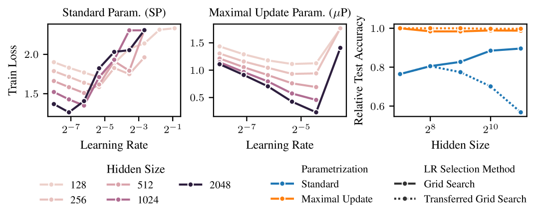
Figure 3: Hyperparameter Transfer. When scaling the size of a neural network, one has to re-tune the hyperparameters, such as the learning rate, when using the standard parametrization (SP). The same is true for probabilistic networks as we show here on CIFAR-10 (left). However, when using our proposed extension of the maximal update parametrization ($\mu$P) [34] to probabilistic networks, one can tune the learning rate on a small model and achieve optimal generalization for larger models by “transferring” the optimal learning rate from a smaller model (center and right).

Figure 3 demonstrates that our proposed maximal update parametrization enables hyperparameter transfer in a probabilistic model. We train two-hidden-layer MLPs on CIFAR10, using a low rank covariance in the final two layers. Under standard parametrization (left panel), the learning rate that results in the smallest training loss decreases with hidden size. In contrast, under $\mu$P (middle panel), it remains the same across hidden sizes. The right panel of Fig. 3 demonstrates the practical implications for model selection. For each parametrization and each hidden size $D$, we select the learning rate based on a grid search. In “transferred grid search” we do a grid search using the smallest model (hidden size 128) and transfer the best validating learning rate to the hidden size $D$ model, whereas in “grid search” we perform the grid search on the hidden size $D$ model. Relative to the test accuracy of the best performing model across learning rate and parametrization, we see that (a) $\mu$P outperforms SP, though the gap decreases with hidden size, and (b) the transfer strategy works well for $\mu$P but poorly for SP once the hidden size exceeds 256.

The $\mu$P parametrization ensures stability and feature learning. Since we interpret the initialization as a prior, which we emphasize is fully theoretically justified in the case of a linear model, this suggests a new approach to designing priors over neural networks. Instead of eliciting beliefs about the relative likelihood of weights or functions, consider how the optimization process evolves the initial parameters and whether desirable properties, like feature learning, will be preserved.

3.5 Related Work

Variational inference in the context of Bayesian deep learning has seen rapid development in recent years [37, 38, 39, 40, 41, 42]. Using a Wasserstein regularizer [27] in the context of generalized VI [26] is arguably most related to our work, given our theoretical results. Structure in the variational parameters has always played an important role for computational reasons [43, 44, 31] and often only a few layers are treated probabilistically [32], with some methods only considering the last layer, effectively treating the neural network as a feature extractor [45, 46]. The Laplace approximation if applied in the last-layer also falls under this category, which has the advantage that it can be applied post-hoc [47, 48, 13, 49, 50, 51, 52, 53, 54]. Deep ensembles repeat the standard training process using multiple random initializations [55, 56] and have been linked to Bayesian methods [57, 58] with certain caveats [59, 60]. While we use SGD only to optimize the variational parameters and arguably average over samples by using momentum, SGD has also been used widely to directly approximate samples from a target distribution [61, 57, 62, 63]. Our theoretical analysis extends recent developments on the implicit bias of overparameterized linear models [4, 7, 5] to the probabilistic setting. For classification, works have focused on convergence rates [6], SGD [7], SGD with momentum [8], and the multiclass setting [10]. Results on the implicit bias of neural network training [22] often assume large widths [64, 9, 65, 66, 67] allowing similar arguments as for linear models. The former is exemplified by the neural tangent parametrization, under which neural networks behave like kernel methods in the infinite width limit [68]. Yang et al. [66, 67, 36, 34] developed an alternative parameterization that still admits feature learning in the infinite width limit, which we extended to the case of variational networks.

4 Theoretical Analysis

Consider an overparameterized linear model with a Gaussian prior, which is trained via maximum expected log-likelihood using (stochastic) gradient descent. We will show that, in both regression (Theorem 1) and binary classification (Theorem 2), our approach can be understood as generalized variational inference with a 2-Wasserstein regularizer, which penalizes deviation from the prior. These theoretical results directly recover analogous results for non-probabilistic models [5, 4].

4.1 Linear Regression

Theorem 1 (Implicit Bias in Regression)

Let $f_{\bm{w}}({\bm{x}})={\bm{x}}^{{\mathsf{T}}}{\bm{w}}$ be an overparametrized linear model with $P>N$. Define a Gaussian prior $p({\bm{w}})={\operatorname{\mathcal{N}}\mathopen{}\left({\bm{w}};{\bm{\mu}}_{0},{\bm{S}}_{0}{\bm{S}}_{0}^{\mathsf{T}}\right)}$ and likelihood $p({\bm{y}}\mid{\bm{w}})={\operatorname{\mathcal{N}}\mathopen{}\left({\bm{y}};f_{\bm{w}}({\bm{X}}),\sigma^{2}{\bm{I}}\right)}$ and assume a variational family $q_{{\bm{\theta}}}({\bm{w}})={\operatorname{\mathcal{N}}\mathopen{}\left({\bm{w}};{\bm{\mu}},{\bm{S}}{\bm{S}}^{\mathsf{T}}\right)}$ with ${\bm{\theta}}=({\bm{\mu}},{\bm{S}})$ such that ${\bm{\mu}}\in\mathbb{R}^{P}$ and ${\bm{S}}\in\mathbb{R}^{P\times R}$ where $R\leq P$. If the learning rate sequence $\{\eta_{t}\}_{t}$ is chosen such that the limit point ${\bm{\theta}}_{\star}^{\textnormal{GD}}=\lim_{t\to\infty}{\bm{\theta}}_{t}^{\textnormal{GD}}$ identified by gradient descent, initialized at ${\bm{\theta}}_{0}=({\bm{\mu}}_{0},{\bm{S}}_{0})$, is a (global) minimizer of the expected log-likelihood $\bar{\ell}({\bm{\theta}})$, then

$${\bm{\theta}}_{\star}^{\textnormal{GD}}\in\operatorname*{arg\,min}_{\begin{subarray}{c}{\bm{\theta}}=({\bm{\mu}},{\bm{S}})\\ \textrm{s.t.\@\ }{\bm{\theta}}\in\operatorname*{arg\,min}\bar{\ell}({\bm{\theta}})\end{subarray}}\operatorname{W}_{2}^{2}\mathopen{}\left(q_{{\bm{\theta}}},p\right).$$ (8)

Further, this also holds in the case of stochastic gradient descent and when using momentum.

Proof.

See Section S1.1.1. ∎

Theorem 1 states that, among those variational parameters which minimize the expected loss, SGD (with momentum) converges to the unique variational distribution which is closest in 2-Wasserstein distance to the prior. This characterization of the implicit regularization of SGD as generalized variational inference differs from a standard ELBO objective (2) in VI via the choice of regularizer. Since the variational parameters minimize the expected loss in Equation 8, all samples from the predictive distribution interpolate the training data (see Figure 1(b), right panel), the same way a standard neural network would. In contrast, when training with a KL regularizer, the uncertainty does not collapse at the training data (see Figure 1(b), left panel), in fact a KL regularizer would diverge to infinity for a Gaussian with vanishing variance. Now, for test points that are increasingly out-of-distribution, i.e. less aligned with the span of the training data, the variational predictive matches the prior predictive more closely. Next, we will prove a similar result for binary classification.

4.2 Binary Classification of Linearly Separable Data

Consider a binary classification problem with labels $y_{n}\in\{-1,1\}$, a linear model $f_{\bm{w}}({\bm{x}})={\bm{x}}^{{\mathsf{T}}}{\bm{w}}$ and a variational distribution $q_{{\bm{\theta}}}({\bm{w}})$ with variational parameters ${\bm{\theta}}$. The expected empirical loss is $\textstyle\bar{\ell}({\bm{\theta}})=\sum_{n=1}^{N}\operatorname{\mathbb{E}}_{q_{{\bm{\theta}}}({\bm{w}})}\mathopen{}\left(\ell(y_{n}{\bm{x}}_{n}^{\mathsf{T}}{\bm{w}})\right).$ We assume without loss of generality that all labels are positive, such that $y_{n}=1$, and that the dataset is linearly separable.

Assumption 1

The dataset is linearly separable: $\exists{\bm{v}}_{\star}$ such that $\forall n:{\bm{v}}_{\star}^{\mathsf{T}}{\bm{x}}_{n}>0$.

Define $\hat{{\bm{\mu}}}$ to be the $L_{2}$ max margin vector, i.e. the solution to the hard margin SVM:

$$\hat{{\bm{\mu}}}=\operatorname*{arg\,min}_{{\bm{\mu}}\in\mathbb{R}^{P}}\|{\bm{\mu}}\|_{2}^{2}\quad\textrm{\ s.t.\@\ }\quad{\bm{\mu}}^{\mathsf{T}}{\bm{x}}_{n}\geq 1,$$ (9)

and the set of support vectors $\mathcal{S}=\operatorname*{arg\,min}_{n\in[N]}{\bm{x}}_{n}^{\mathsf{T}}\hat{{\bm{\mu}}}$ indexing those data points that lie on the margin. We adapt the following additional assumption from [7], which can be omitted at expense of simplicity as we show in Section S1.2.

Assumption 2

The SVM support vectors span the dataset: $\operatorname{span}(\{{\bm{x}}_{n}\}_{n\in[N]})=\operatorname{span}(\{{\bm{x}}_{n}\}_{n\in\mathcal{S}})$.

We can now characterize the implicit bias in the case of binary classification.

Theorem 2 (Implicit Bias in Binary Classification)

Let $f_{\bm{w}}({\bm{x}})={\bm{x}}^{{\mathsf{T}}}{\bm{w}}$ be an (overparametrized) linear model and define a Gaussian prior $p({\bm{w}})={\operatorname{\mathcal{N}}\mathopen{}\left({\bm{w}};{\bm{\mu}}_{0},{\bm{S}}_{0}{\bm{S}}_{0}^{\mathsf{T}}\right)}$. Assume a variational distribution $\smash{q_{{\bm{\theta}}}({\bm{w}})={\operatorname{\mathcal{N}}\mathopen{}\left({\bm{w}};{\bm{\mu}},{\bm{S}}{\bm{S}}^{\mathsf{T}}\right)}}$ over the weights $\smash{{\bm{w}}\in\mathbb{R}^{P}}$ with variational parameters ${\bm{\theta}}=({\bm{\mu}},{\bm{S}})$ such that ${\bm{S}}\in\mathbb{R}^{P\times R}$ and $R\leq P$. Assume we are using the exponential loss $\ell(u)=\exp(-u)$ and optimize the expected empirical loss $\bar{\ell}({\bm{\theta}})$ via gradient descent initialized at the prior, i.e. ${\bm{\theta}}_{0}=({\bm{\mu}}_{0},{\bm{S}}_{0})$, with a sufficiently small learning rate $\eta$. Then for almost any dataset which is linearly separable (Assumption 1) and for which the support vectors span the data (Assumption 2), the rescaled gradient descent iterates (rGD)

$$\textstyle{\bm{\theta}}_{t}^{\textnormal{rGD}}=({\bm{\mu}}_{t}^{\textnormal{rGD}},{\bm{S}}_{t}^{\textnormal{rGD}})=\left(\frac{1}{\log(t)}{\bm{\mu}}_{t}^{\textnormal{GD}}+{\bm{P}}_{\textup{null}({\bm{X}})}{\bm{\mu}}_{0},{\bm{S}}_{t}^{\textnormal{GD}}\right)$$ (10)

converge to a limit point ${\bm{\theta}}_{\star}^{\textnormal{rGD}}=\lim_{t\to\infty}{\bm{\theta}}_{t}^{\textnormal{rGD}}$ for which it holds that

$${\bm{\theta}}_{\star}^{\textnormal{rGD}}\in\operatorname*{arg\,min}_{\begin{subarray}{c}{\bm{\theta}}=({\bm{\mu}},{\bm{S}})\\ \textrm{s.t.\@\ }{\bm{\theta}}\in\Theta_{\star}\end{subarray}}\operatorname{W}_{2}^{2}\mathopen{}\left(q_{{\bm{\theta}}},p\right).$$ (11)

where the feasible set $\Theta_{\star}=\{({\bm{\mu}},{\bm{S}})\mid{\bm{P}}_{\textup{range}({\bm{X}}^{\mathsf{T}})}{\bm{\mu}}=\hat{{\bm{\mu}}}\quad\textrm{and}\quad\forall n:\operatorname{Var}_{q_{{\bm{\theta}}}}\mathopen{}\left(f_{\bm{w}}({\bm{x}}_{n})\right)=0\}$ consists of mean parameters which, if projected onto the training data, are equivalent to the $L_{2}$ max margin vector and covariance parameters such that there is no uncertainty at training data.

Proof.

See Section S1.2. ∎

Theorem 2 states that the mean parameters ${\bm{\mu}}_{t}$ converge to the $L_{2}$ max-margin vector $\hat{{\bm{\mu}}}$ in the span of the training data, i.e. the data manifold, and there uncertainty collapses to zero. This is analogous to the regression case, where zero training loss enforces interpolation of the training data. In the null space of the training data, i.e. off of the data manifold, the model falls back on the prior as enforced by the 2-Wasserstein distance. The assumption of an exponential loss is standard in the literature and we expect this to extend to (binary) cross-entropy in the same way it does in results for standard neural networks [4, 6, 7, 8, 10]. Similarly, we conjecture that Theorem 2 can be extended to SGD with momentum [[, cf. ]]Nacson2019StochasticGradient,Wang2022DoesMomentum. While Theorem 2 is similar to Theorem 1, there are some subtle differences. First, the feasible set for the minimization problem in Equation 11 is not the set of minima of the expected loss. This is because the exponential function does not have an optimum in contrast to a quadratic function. However, the sequence of variational parameters identified by gradient descent still satisfies $\lim_{t\to\infty}\bar{\ell}({\bm{\theta}}_{t})=0$. Second, without transformation of the mean parameters, the exponential loss results in the mean parameters being unbounded. This necessitates the transformation in Equation 10 as we explain in detail in Section S1.3.

5 Experiments

We benchmark the generalization and robustness of our approach, Implicit Bias VI (IBVI), against standard neural networks and several baselines for uncertainty quantification, namely Temperature Scaling (TS) [69], Deep Ensembles (DE) [55], Weight-Space VI (WSVI) [37, 38] and Laplace (LA-GS) & Laplace (LA-ML) [47, 48, 52], on a set of standard benchmark datasets for image classification and robustness to input corruptions. We use a convolutional architecture (either LeNet5 [70] or ResNet34 [71]) throughout, which, for all datasets but MNIST, is initialized with pretrained weights in all layers except for the input and output layer. All models were trained with SGD with momentum $\gamma=0.9$ and a batch size of $N_{b}=128$ for $200$ epochs in single precision on an NVIDIA GH200 GPU. Results shown are averaged across five random seeds. A detailed description of the datasets, metrics, models and training can be found in Section S3.

In-Distribution Generalization and Uncertainty Quantification In order to assess the in-distribution generalization, we measure the test error, negative log-likelihood (NLL) and calibration error (ECE) on MNIST, CIFAR10, CIFAR100 and TinyImageNet. As Figure 4 shows for CIFAR100, and Figure S10 for all datasets, the test error for post-hoc methods (TS, LA-GS, LA-ML) is unchanged. As expected, IBVI also performs similarly with only Ensembles providing an increase in accuracy, but at substantial memory overhead compared to most other approaches. In-distribution uncertainty quantification measured in terms of NLL is improved substantially by TS, DE and IBVI with only LA showing occasional worsening of NLL compared to the base model. As the full results in Figure S10 show, TS, DE and IBVI also consistently are the best calibrated. As described in Section 3.3, for IBVI we train with a single sample only and a probabilistic input and output layer with low-rank covariance, reducing the computational overhead compared to a standard neural network to as little as $\approx 10\%$ both in time and memory (see Figure 4). See Section S3.3.2 for the full experimental results including using different parametrizations (SP vs $\mu$P).

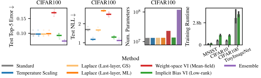
Figure 4: In-distribution generalization and uncertainty quantification. Implicit Bias VI (IBVI) has similar test error to other Bayesian deep learning approaches and achieves competitive uncertainty quantification on in-distribution data. While ensembles have improved accuracy, they come at an additional memory overhead. Training a probabilistic model via IBVI has only a minor computational overhead during training, both in time and memory, over standard deep learning.

Robustness to Input Corruptions We evaluate the robustness of the different models on MNISTC [72], CIFAR10C, CIFAR100C and TinyImageNetC [73]. These are corrupted versions of the original datasets, where the images are modified via a set of $15$ corruptions, such as impulse noise, blur, pixelation etc. We selected the maximum severity for each corruption and averaged the performance across all. As expected, the performance of all models drops compared to the in-distribution performance measured on the standard test sets as Figure 5 shows. Besides DE which consistently show lower test error, also IBVI sometimes shows improved accuracy on corrupted data compared to all other approaches, especially when using the maximal update parametrization (see Figure S12). TS, DE and IBVI perform consistently well in terms of uncertainty quantification (both for NLL and ECE) across all datasets. However, compared to the in-distribution setting IBVI has better uncertainty quantification than the Ensemble across all datasets.

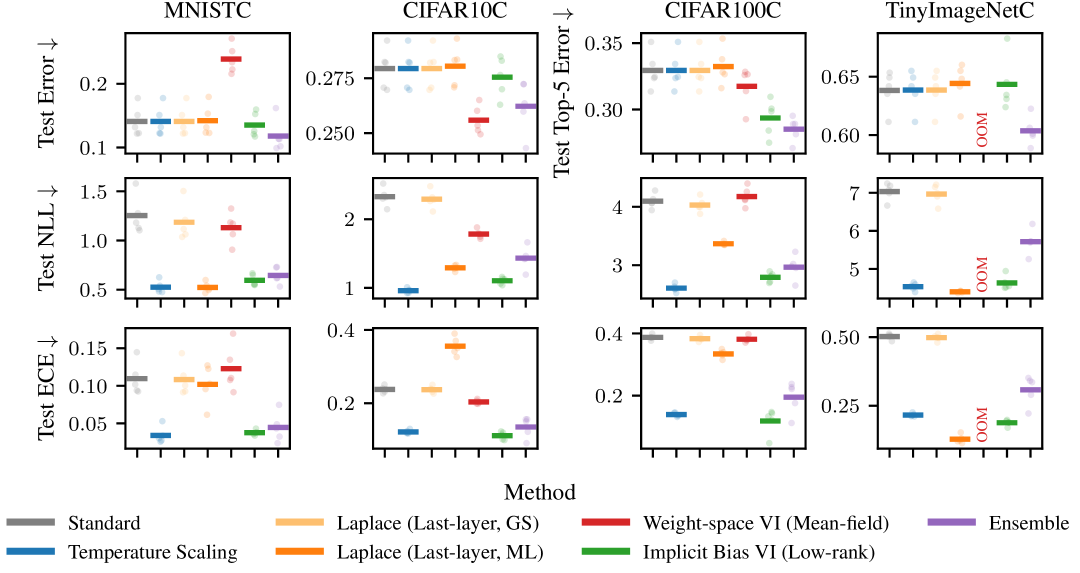
Figure 5: Generalization on robustness benchmark problems. When comparing different methods for Bayesian deep learning with regards to robustness to 15 different input corruptions, our approach, Implicit Bias VI, consistently has competitive uncertainty quantification across different datasets and metrics without sacrificing accuracy compared to a non-probabilistic network.

Limitations Compared to standard neural networks, when training via Implicit Bias VI, we observed that often lower learning rates were necessary due to the additional stochasticity in the objective (see also Section 3.3). While this does not have a significant impact on generalization, the models sometimes require slightly more epochs to achieve similar in-distribution performance to standard neural networks. Effectively, in the beginning of training it takes a bit more time for IBVI to become sufficiently certain about those features which are critical for in-distribution performance. This also means that folk knowledge on learning rate settings for specific architectures may not immediately transfer. In the experiments we train models with probabilistic in- and output layers with our approach, but we have so far not explored other covariance structures or where in the network probabilistic layers are most beneficial. While there is some theoretical evidence this may be sufficient [32], we believe there is potential for improvement. Beyond the prior induced by a choice of parametrization, we did not experiment with more informative or learned priors, which could potentially give significant performance improvements on certain tasks [15].

6 Conclusion

In this paper, we demonstrated how to exploit the implicit regularization of (stochastic) gradient descent for variational deep learning, as opposed to relying on explicit regularization. We rigorously characterized this implicit bias for an overparametrized linear model and showed that our approach is equivalent to generalized variational inference with a 2-Wasserstein regularizer at reduced computational cost. We demonstrated the importance of parameterization and how it impacts the inductive bias via the initialization — thus conferring desirable properties such as learning rate transfer. Lastly, we empirically demonstrated competitive performance with state-of-the-art methods for Bayesian deep learning on a set of in- and out-of-distribution benchmarks with minimal computational overhead over standard deep learning. In principle, our approach is not restricted to Gaussian variational families and should seemlessly extend to location-scale families, which could further improve performance. Finally, it would be interesting to explore connections between Implicit Bias VI and Bayesian deep learning in function-space [[, e.g.,]]Burt2020UnderstandingVariational,Wild2022GeneralizedVariational,Qiu2023ShouldWe,Rudner2023TractableFunctionSpace,Cinquin2024FSPLaplaceFunctionSpace.

[supplementary]

Supplementary Material

This supplementary material contains additional results and proofs for all theoretical statements. References referring to sections, equations or theorem-type environments within this document are prefixed with ‘S’, while references to, or results from, the main paper are stated as is.

[supplementary]1

S1 Theoretical Results

Lemma S1

Let $q({\bm{w}})={\operatorname{\mathcal{N}}\mathopen{}\left({\bm{w}};{\bm{\mu}},{\bm{\Sigma}}\right)}$, $p({\bm{w}})={\operatorname{\mathcal{N}}\mathopen{}\left({\bm{w}};{\bm{\mu}}_{0},{\bm{\Sigma}}_{0}\right)}$ such that ${\bm{\mu}},{\bm{\mu}}_{0}\in\mathbb{R}^{P}$, ${\bm{\Sigma}},{\bm{\Sigma}}_{0}\in\mathbb{R}^{P\times P}$ positive semi-definite and let ${\bm{V}}_{A}\in\mathbb{R}^{P\times N}$, ${\bm{V}}_{B}\in\mathbb{R}^{P\times(P-N)}$ be matrices with pairwise orthonormal columns that together define an orthonormal basis of $\mathbb{R}^{P}$, i.e. for ${\bm{V}}=\begin{bmatrix}{\bm{V}}_{A}&{\bm{V}}_{B}\end{bmatrix}$ it holds that ${\bm{V}}{\bm{V}}^{\mathsf{T}}={\bm{V}}^{\mathsf{T}}{\bm{V}}={\bm{I}}$ and $\operatorname{span}({\bm{V}})=\mathbb{R}^{P}$. Assume further that

$${\bm{V}}_{A}^{\mathsf{T}}{\bm{\Sigma}}{\bm{V}}_{A}={\bm{0}},$$ (S12)

then the squared 2-Wasserstein distance is given by

$$\operatorname{W}_{2}^{2}\mathopen{}\left(q,p\right)=\left\lVert{\bm{V}}_{A}^{\mathsf{T}}{\bm{\mu}}-{\bm{V}}_{A}^{\mathsf{T}}{\bm{\mu}}_{0}\right\rVert_{2}^{2}+\operatorname{W}_{2}^{2}\mathopen{}\left({\operatorname{\mathcal{N}}\mathopen{}\left({\bm{V}}_{B}^{\mathsf{T}}{\bm{\mu}},{\bm{V}}_{B}^{\mathsf{T}}{\bm{\Sigma}}{\bm{V}}_{B}\right)},{\operatorname{\mathcal{N}}\mathopen{}\left({\bm{V}}_{B}^{\mathsf{T}}{\bm{\mu}}_{0},{\bm{V}}_{B}^{\mathsf{T}}{\bm{\Sigma}}_{0}{\bm{V}}_{B}\right)}\right)+C,$$ (S13)

where the constant $C$ is independent of $({\bm{\mu}},{\bm{\Sigma}})$.

Proof.

Consider the matrix

$${\bm{V}}^{\mathsf{T}}{\bm{\Sigma}}{\bm{V}}=\begin{bmatrix}{\bm{0}}_{N\times N}&{\bm{V}}_{A}^{\mathsf{T}}{\bm{\Sigma}}{\bm{V}}_{B}\\ {\bm{V}}_{B}^{\mathsf{T}}{\bm{\Sigma}}{\bm{V}}_{A}&{\bm{V}}_{B}^{\mathsf{T}}{\bm{\Sigma}}{\bm{V}}_{B}\end{bmatrix}.$$

Since ${\bm{V}}^{\mathsf{T}}{\bm{\Sigma}}{\bm{V}}$ is symmetric positive semi-definite, its off-diagonal block ${\bm{V}}_{A}^{\mathsf{T}}{\bm{\Sigma}}{\bm{V}}_{B}$ satisfies

$$({\bm{I}}-{\bm{0}}{\bm{0}}^{\dagger}){\bm{V}}_{A}^{\mathsf{T}}{\bm{\Sigma}}{\bm{V}}_{B}={\bm{0}}\iff{\bm{V}}_{A}^{\mathsf{T}}{\bm{\Sigma}}{\bm{V}}_{B}={\bm{0}}$$

by [77, A5.5, ]. Therefore, we have

$${\bm{V}}^{\mathsf{T}}{\bm{\Sigma}}{\bm{V}}=\begin{bmatrix}{\bm{0}}_{N\times N}&{\bm{V}}_{A}^{\mathsf{T}}{\bm{\Sigma}}{\bm{V}}_{B}\\ {\bm{V}}_{B}^{\mathsf{T}}{\bm{\Sigma}}{\bm{V}}_{A}&{\bm{V}}_{B}^{\mathsf{T}}{\bm{\Sigma}}{\bm{V}}_{B}\end{bmatrix}=\begin{bmatrix}{\bm{0}}_{N\times N}&{\bm{0}}_{N\times(P-N)}\\ {\bm{0}}_{(P-N)\times N}&{\bm{V}}_{B}^{\mathsf{T}}{\bm{\Sigma}}{\bm{V}}_{B}\end{bmatrix}.$$ (S14)

The squared 2-Wasserstein distance between $q({\bm{w}})$ and $p({\bm{w}})$ is given by

$$\operatorname{W}_{2}^{2}\mathopen{}\left(q,p\right)=\lVert{\bm{\mu}}-{\bm{\mu}}_{0}\rVert_{2}^{2}+\operatorname{tr}({\bm{\Sigma}}-2({\bm{\Sigma}}^{\frac{1}{2}}{\bm{\Sigma}}_{0}{\bm{\Sigma}}^{\frac{1}{2}})^{\frac{1}{2}}+{\bm{\Sigma}}_{0}).$$

For the squared norm term it holds by unitary invariance of $\lVert\cdot\rVert_{2}$ that

$$\lVert{\bm{\mu}}-{\bm{\mu}}_{0}\rVert_{2}^{2} =\lVert{\bm{V}}^{\mathsf{T}}({\bm{\mu}}-{\bm{\mu}}_{0})\rVert_{2}^{2}=\left\lVert\begin{bmatrix}{\bm{V}}_{A}^{\mathsf{T}}({\bm{\mu}}-{\bm{\mu}}_{0})\\ {\bm{V}}_{B}^{\mathsf{T}}({\bm{\mu}}-{\bm{\mu}}_{0})\end{bmatrix}\right\rVert_{2}^{2}=\left\lVert{\bm{V}}_{A}^{\mathsf{T}}{\bm{\mu}}-{\bm{V}}_{A}^{\mathsf{T}}{\bm{\mu}}_{0}\right\rVert_{2}^{2}+\left\lVert{\bm{V}}_{B}^{\mathsf{T}}{\bm{\mu}}-{\bm{V}}_{B}^{\mathsf{T}}{\bm{\mu}}_{0}\right\rVert_{2}^{2}.$$

Now for the trace term we have that

$$\operatorname{tr}({\bm{V}}{\bm{V}}^{\mathsf{T}}({\bm{\Sigma}}-2({\bm{\Sigma}}^{\frac{1}{2}}{\bm{\Sigma}}_{0}{\bm{\Sigma}}^{\frac{1}{2}})^{\frac{1}{2}}+{\bm{\Sigma}}_{0}))$$ (S15)

$$=\operatorname{tr}({\bm{V}}^{\mathsf{T}}{\bm{\Sigma}}{\bm{V}})-2\operatorname{tr}({\bm{V}}^{\mathsf{T}}({\bm{\Sigma}}^{\frac{1}{2}}{\bm{\Sigma}}_{0}{\bm{\Sigma}}^{\frac{1}{2}})^{\frac{1}{2}}{\bm{V}})+\operatorname{tr}({\bm{V}}^{\mathsf{T}}{\bm{\Sigma}}_{0}{\bm{V}})$$

$$=\operatorname{tr}({\bm{V}}_{A}^{\mathsf{T}}{\bm{\Sigma}}{\bm{V}}_{A})+\operatorname{tr}({\bm{V}}_{B}^{\mathsf{T}}{\bm{\Sigma}}{\bm{V}}_{B})+\operatorname{tr}({\bm{V}}_{A}^{\mathsf{T}}{\bm{\Sigma}}_{0}{\bm{V}}_{A})+\operatorname{tr}({\bm{V}}_{B}^{\mathsf{T}}{\bm{\Sigma}}_{0}{\bm{V}}_{B})-2\operatorname{tr}({\bm{V}}^{\mathsf{T}}({\bm{\Sigma}}^{\frac{1}{2}}{\bm{\Sigma}}_{0}{\bm{\Sigma}}^{\frac{1}{2}})^{\frac{1}{2}}{\bm{V}})$$

$$\overset{c}{=}\operatorname{tr}({\bm{V}}_{B}^{\mathsf{T}}{\bm{\Sigma}}{\bm{V}}_{B})+\operatorname{tr}({\bm{V}}_{B}^{\mathsf{T}}{\bm{\Sigma}}_{0}{\bm{V}}_{B})-2\operatorname{tr}({\bm{V}}^{\mathsf{T}}({\bm{\Sigma}}^{\frac{1}{2}}{\bm{\Sigma}}_{0}{\bm{\Sigma}}^{\frac{1}{2}})^{\frac{1}{2}}{\bm{V}})$$

where we used Eq. S12 and $\overset{c}{=}$ denotes equality up to constants independent of $({\bm{\mu}},{\bm{\Sigma}})$.

Now by Eq. S14, we have that ${\bm{\Sigma}}={\bm{V}}_{B}{\bm{M}}{\bm{V}}_{B}^{\mathsf{T}}$ for ${\bm{M}}={\bm{V}}_{B}^{\mathsf{T}}{\bm{\Sigma}}{\bm{V}}_{B}$ and its unique principal square root is given by ${\bm{\Sigma}}^{\frac{1}{2}}={\bm{V}}_{B}{\bm{M}}^{\frac{1}{2}}{\bm{V}}_{B}^{\mathsf{T}}$ since

$$({\bm{V}}_{B}{\bm{M}}^{\frac{1}{2}}{\bm{V}}_{B}^{\mathsf{T}})({\bm{V}}_{B}{\bm{M}}^{\frac{1}{2}}{\bm{V}}_{B}^{\mathsf{T}})={\bm{V}}_{B}{\bm{M}}^{\frac{1}{2}}{\bm{I}}_{(P-N)\times(P-N)}{\bm{M}}^{\frac{1}{2}}{\bm{V}}_{B}^{\mathsf{T}}={\bm{\Sigma}}.$$

It also holds that the unique principal square root

$$({\bm{\Sigma}}^{\frac{1}{2}}{\bm{\Sigma}}_{0}{\bm{\Sigma}}^{\frac{1}{2}})^{\frac{1}{2}}={\bm{V}}_{B}({\bm{M}}^{\frac{1}{2}}{\bm{V}}_{B}^{\mathsf{T}}{\bm{\Sigma}}_{0}{\bm{V}}_{B}{\bm{M}}^{\frac{1}{2}})^{\frac{1}{2}}{\bm{V}}_{B}^{\mathsf{T}}$$

since direct calculation gives

$$({\bm{V}}_{B}({\bm{M}}^{\frac{1}{2}} {\bm{V}}_{B}^{\mathsf{T}}{\bm{\Sigma}}_{0}{\bm{V}}_{B}{\bm{M}}^{\frac{1}{2}})^{\frac{1}{2}}{\bm{V}}_{B}^{\mathsf{T}})({\bm{V}}_{B}({\bm{M}}^{\frac{1}{2}}{\bm{V}}_{B}^{\mathsf{T}}{\bm{\Sigma}}_{0}{\bm{V}}_{B}{\bm{M}}^{\frac{1}{2}})^{\frac{1}{2}}{\bm{V}}_{B}^{\mathsf{T}})$$

$$={\bm{V}}_{B}{\bm{M}}^{\frac{1}{2}}{\bm{V}}_{B}^{\mathsf{T}}{\bm{\Sigma}}_{0}{\bm{V}}_{B}{\bm{M}}^{\frac{1}{2}}{\bm{V}}_{B}^{\mathsf{T}}={\bm{\Sigma}}^{\frac{1}{2}}{\bm{\Sigma}}_{0}{\bm{\Sigma}}^{\frac{1}{2}}.$$

Therefore we have that

$$\operatorname{tr}({\bm{V}}^{\mathsf{T}}({\bm{\Sigma}}^{\frac{1}{2}}{\bm{\Sigma}}_{0}{\bm{\Sigma}}^{\frac{1}{2}})^{\frac{1}{2}}{\bm{V}})=\operatorname{tr}({\bm{V}}^{\mathsf{T}}{\bm{V}}_{B}({\bm{M}}^{\frac{1}{2}}{\bm{V}}_{B}^{\mathsf{T}}{\bm{\Sigma}}_{0}{\bm{V}}_{B}{\bm{M}}^{\frac{1}{2}})^{\frac{1}{2}}{\bm{V}}_{B}^{\mathsf{T}}{\bm{V}})\\ =\operatorname{tr}(({\bm{M}}^{\frac{1}{2}}{\bm{V}}_{B}^{\mathsf{T}}{\bm{\Sigma}}_{0}{\bm{V}}_{B}{\bm{M}}^{\frac{1}{2}})^{\frac{1}{2}}).$$

Putting it all together we obtain

$$\operatorname{W}_{2}^{2}\mathopen{}\left(q,p\right) \overset{c}{=}\left\lVert{\bm{V}}_{A}^{\mathsf{T}}{\bm{\mu}}-{\bm{V}}_{A}^{\mathsf{T}}{\bm{\mu}}_{0}\right\rVert_{2}^{2}+\left\lVert{\bm{V}}_{B}^{\mathsf{T}}{\bm{\mu}}-{\bm{V}}_{B}^{\mathsf{T}}{\bm{\mu}}_{0}\right\rVert_{2}^{2}+\operatorname{tr}({\bm{V}}_{B}^{\mathsf{T}}{\bm{\Sigma}}{\bm{V}}_{B})+\operatorname{tr}({\bm{V}}_{B}^{\mathsf{T}}{\bm{\Sigma}}_{0}{\bm{V}}_{B})-2\operatorname{tr}({\bm{V}}^{\mathsf{T}}({\bm{\Sigma}}^{\frac{1}{2}}{\bm{\Sigma}}_{0}{\bm{\Sigma}}^{\frac{1}{2}})^{\frac{1}{2}}{\bm{V}})$$

$$=\left\lVert{\bm{V}}_{A}^{\mathsf{T}}{\bm{\mu}}-{\bm{V}}_{A}^{\mathsf{T}}{\bm{\mu}}_{0}\right\rVert_{2}^{2}+\left\lVert{\bm{V}}_{B}^{\mathsf{T}}{\bm{\mu}}-{\bm{V}}_{B}^{\mathsf{T}}{\bm{\mu}}_{0}\right\rVert_{2}^{2}+\operatorname{tr}({\bm{V}}_{B}^{\mathsf{T}}{\bm{\Sigma}}{\bm{V}}_{B})+\operatorname{tr}({\bm{V}}_{B}^{\mathsf{T}}{\bm{\Sigma}}_{0}{\bm{V}}_{B})-2\operatorname{tr}(({\bm{M}}^{\frac{1}{2}}{\bm{V}}_{B}^{\mathsf{T}}{\bm{\Sigma}}_{0}{\bm{V}}_{B}{\bm{M}}^{\frac{1}{2}})^{\frac{1}{2}})$$

$$=\left\lVert{\bm{V}}_{A}^{\mathsf{T}}{\bm{\mu}}-{\bm{V}}_{A}^{\mathsf{T}}{\bm{\mu}}_{0}\right\rVert_{2}^{2}+\operatorname{W}_{2}^{2}\mathopen{}\left({\operatorname{\mathcal{N}}\mathopen{}\left({\bm{V}}_{B}^{\mathsf{T}}{\bm{\mu}},{\bm{V}}_{B}^{\mathsf{T}}{\bm{\Sigma}}{\bm{V}}_{B}\right)},{\operatorname{\mathcal{N}}\mathopen{}\left({\bm{V}}_{B}^{\mathsf{T}}{\bm{\mu}}_{0},{\bm{V}}_{B}^{\mathsf{T}}{\bm{\Sigma}}_{0}{\bm{V}}_{B}\right)}\right)$$

which completes the proof. ∎

S1.1 Overparametrized Linear Regression

S1.1.1 Characterization of Implicit Bias (Proof of Theorem 1)

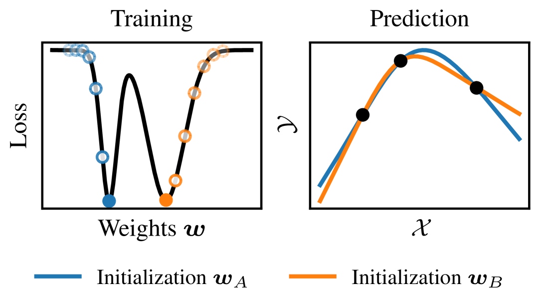
(a) NN trained with no explicit regularization.

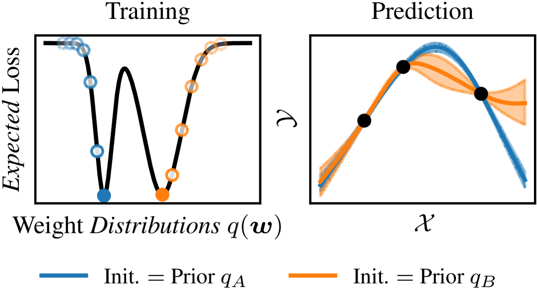
(b) BNN trained with no explicit regularization.

Figure S1: Implicit regularization in standard neural networks versus in probabilistic networks. Left panels: A NN can obtain one of two global minima of the loss. Optimization of the weights will implicitly regularize towards one or the other. Right panels: Analogously, a distribution over NNs can obtain one of two global minima of the expected loss. Optimization of the distribution over the weights will implicitly regularize towards one or the other. Our approach uses this implicit regularization instead of an explicit regularization to a prior.

See 1

Proof.

Let ${\bm{\theta}}_{\star}=({\bm{\mu}}_{\star},{\bm{S}}_{\star})$ be a minimizer of $\bar{\ell}({\bm{\theta}})$. By assumption it holds that the expected negative log-likelihood is equal to the following non-negative loss function up to an additive constant:

$$\bar{\ell}({\bm{\theta}}) =\operatorname{\mathbb{E}}_{q_{{\bm{\theta}}}({\bm{w}})}\mathopen{}\left(\ell({\bm{y}},f_{\bm{w}}({\bm{X}}))\right)=\operatorname{\mathbb{E}}_{q_{{\bm{\theta}}}({\bm{w}})}\mathopen{}\left(-\log p({\bm{y}}\mid{\bm{w}})\right)$$

$$\overset{c}{=}\frac{1}{2\sigma^{2}}\operatorname{\mathbb{E}}_{q_{{\bm{\theta}}}({\bm{w}})}\mathopen{}\left(\lVert{\bm{y}}-{\bm{X}}{\bm{w}}\rVert_{2}^{2}\right)$$

$$=\frac{1}{2\sigma^{2}}\big{(}\lVert{\bm{y}}-{\bm{X}}{\bm{\mu}}\rVert_{2}^{2}+\operatorname{tr}({\bm{X}}{\bm{\Sigma}}{\bm{X}}^{\mathsf{T}})\big{)}\geq 0,$$

where ${\bm{\Sigma}}={\bm{S}}{\bm{S}}^{\mathsf{T}}$ and non-negativity follows from ${\bm{\Sigma}}$ being symmetric positive semi-definite. Therefore any (global) minimizer ${\bm{\theta}}_{\star}=({\bm{\mu}}_{\star},{\bm{\Sigma}}_{\star})$ necessarily satisfies

$$\lVert{\bm{y}}-{\bm{X}}{\bm{\mu}}_{\star}\rVert_{2}^{2} =0,$$ (S16)

$$\operatorname{tr}({\bm{X}}{\bm{\Sigma}}_{\star}{\bm{X}}^{\mathsf{T}}) =0.$$ (S17)

Let ${\bm{V}}=\begin{bmatrix}{\bm{V}}_{\textnormal{range}}&{\bm{V}}_{\textnormal{null}}\end{bmatrix}\in\mathbb{R}^{P\times P}$ be the orthonormal matrix of right singular vectors of ${\bm{X}}={\bm{U}}{\bm{\Lambda}}{\bm{V}}^{\mathsf{T}}$, where ${\bm{V}}_{\textnormal{range}}\in\mathbb{R}^{P\times N}$ and ${\bm{V}}_{\textnormal{null}}\in\mathbb{R}^{P\times(P-N)}$. Since ${\bm{X}}\in\mathbb{R}^{N\times P}$ and we are in the overparametrized regime, i.e. $P>N$, the optimal mean parameter decomposes into the least-squares solution and a null space contribution

$${\bm{\mu}}_{\star}={\bm{V}}_{\textnormal{range}}{\bm{u}}_{\star}+{\bm{V}}_{\textnormal{null}}{\bm{z}}={\bm{X}}^{\dagger}{\bm{y}}+{\bm{V}}_{\textnormal{null}}{\bm{z}}.$$ (S18)

Furthermore, it holds for positive semi-definite ${\bm{\Sigma}}\in\mathbb{R}^{P\times P}$ that

$$0\leq\operatorname{tr}({\bm{X}}{\bm{\Sigma}}{\bm{X}}^{\mathsf{T}}) =\operatorname{tr}({\bm{U}}{\bm{\Lambda}}{\bm{V}}^{\mathsf{T}}{\bm{\Sigma}}{\bm{V}}{\bm{\Lambda}}{\bm{U}}^{\mathsf{T}})=\operatorname{tr}({\bm{\Lambda}}{\bm{V}}^{\mathsf{T}}{\bm{\Sigma}}{\bm{V}}{\bm{\Lambda}})$$

$$=\operatorname{tr}(\begin{bmatrix}{\bm{\Lambda}}_{N\times N}&{\bm{0}}\end{bmatrix}\begin{bmatrix}{\bm{V}}_{\textnormal{range}}^{\mathsf{T}}{\bm{\Sigma}}{\bm{V}}_{\textnormal{range}}&*\\ *&*\end{bmatrix}\begin{bmatrix}{\bm{\Lambda}}_{N\times N}\\ {\bm{0}}\end{bmatrix})$$

$$=\operatorname{tr}({\bm{\Lambda}}_{N\times N}{\bm{V}}_{\textnormal{range}}^{\mathsf{T}}{\bm{\Sigma}}{\bm{V}}_{\textnormal{range}}{\bm{\Lambda}}_{N\times N})$$

$$=\sum_{i=1}^{N}\lambda_{i}^{2}[{\bm{V}}_{\textnormal{range}}^{\mathsf{T}}{\bm{\Sigma}}{\bm{V}}_{\textnormal{range}}]_{ii}$$

where $\lambda_{i}^{2}>0$ are the squared singular values of ${\bm{X}}$, which are strictly positive since $\operatorname{rank}({\bm{X}})=N$. Therefore using Equation S17 any global minimizer necessarily satisfies $[{\bm{V}}_{\textnormal{range}}^{\mathsf{T}}{\bm{\Sigma}}_{\star}{\bm{V}}_{\textnormal{range}}]_{ii}=0$ for $i\in\{1,\dots,N\}$. Now since ${\bm{V}}_{\textnormal{range}}^{\mathsf{T}}{\bm{\Sigma}}_{\star}{\bm{V}}_{\textnormal{range}}$ is symmetric positive semi-definite and its diagonal is zero, so is its trace and therefore the sum of its non-negative eigenvalues is necessarily zero. Thus all eigenvalues are zero and therefore

$${\bm{V}}_{\textnormal{range}}^{\mathsf{T}}{\bm{\Sigma}}{\bm{V}}_{\textnormal{range}}={\bm{0}}.$$ (S19)

Now by Lemma S1 we have that the squared 2-Wasserstein distance between $q_{{\bm{\theta}}_{\star}}({\bm{w}})={\operatorname{\mathcal{N}}\mathopen{}\left({\bm{w}};{\bm{\mu}}_{\star},{\bm{\Sigma}}_{\star}\right)}$ and the initialization $p({\bm{w}})={\operatorname{\mathcal{N}}\mathopen{}\left({\bm{w}};{\bm{\mu}}_{0},{\bm{\Sigma}}_{0}\right)}$ is given up to a constant independent of $({\bm{\mu}}_{\star},{\bm{\Sigma}}_{\star})$ by

$$\operatorname{W}_{2}\mathopen{}\left(q_{{\bm{\theta}}_{\star}},p\right) \overset{c}{=}\left\lVert{\bm{V}}_{\textrm{range}}^{\mathsf{T}}{\bm{\mu}}_{\star}-{\bm{V}}_{\textrm{range}}^{\mathsf{T}}{\bm{\mu}}_{0}\right\rVert_{2}^{2}+\operatorname{W}_{2}^{2}\mathopen{}\left({\operatorname{\mathcal{N}}\mathopen{}\left({\bm{V}}_{\textrm{null}}^{\mathsf{T}}{\bm{\mu}}_{\star},{\bm{V}}_{\textrm{null}}^{\mathsf{T}}{\bm{\Sigma}}_{\star}{\bm{V}}_{\textrm{null}}\right)},{\operatorname{\mathcal{N}}\mathopen{}\left({\bm{V}}_{\textrm{null}}^{\mathsf{T}}{\bm{\mu}}_{0},{\bm{V}}_{\textrm{null}}^{\mathsf{T}}{\bm{\Sigma}}_{0}{\bm{V}}_{\textrm{null}}\right)}\right)$$

$$=\left\lVert{\bm{X}}^{\dagger}{\bm{y}}-{\bm{V}}_{\textrm{range}}^{\mathsf{T}}{\bm{\mu}}_{0}\right\rVert_{2}^{2}+\operatorname{W}_{2}^{2}\mathopen{}\left({\operatorname{\mathcal{N}}\mathopen{}\left({\bm{V}}_{\textrm{null}}^{\mathsf{T}}{\bm{\mu}}_{\star},{\bm{V}}_{\textrm{null}}^{\mathsf{T}}{\bm{\Sigma}}_{\star}{\bm{V}}_{\textrm{null}}\right)},{\operatorname{\mathcal{N}}\mathopen{}\left({\bm{V}}_{\textrm{null}}^{\mathsf{T}}{\bm{\mu}}_{0},{\bm{V}}_{\textrm{null}}^{\mathsf{T}}{\bm{\Sigma}}_{0}{\bm{V}}_{\textrm{null}}\right)}\right)$$

$$\overset{c}{=}\operatorname{W}_{2}^{2}\mathopen{}\left({\operatorname{\mathcal{N}}\mathopen{}\left({\bm{V}}_{\textrm{null}}^{\mathsf{T}}{\bm{\mu}}_{\star},{\bm{V}}_{\textrm{null}}^{\mathsf{T}}{\bm{\Sigma}}_{\star}{\bm{V}}_{\textrm{null}}\right)},{\operatorname{\mathcal{N}}\mathopen{}\left({\bm{V}}_{\textrm{null}}^{\mathsf{T}}{\bm{\mu}}_{0},{\bm{V}}_{\textrm{null}}^{\mathsf{T}}{\bm{\Sigma}}_{0}{\bm{V}}_{\textrm{null}}\right)}\right)$$

Therefore among variational distributions $q_{{\bm{\theta}}_{\star}}$ with parameters ${\bm{\theta}}_{\star}$ that minimize the expected loss $\bar{\ell}({\bm{\theta}})$, any such ${\bm{\theta}}_{\star}$ that minimizes the squared 2-Wasserstein distance to the prior satisfies

$$(\underbracket{{\bm{V}}_{\textrm{null}}^{\mathsf{T}}{\bm{\mu}}_{\star}}_{\eqqcolon{\bm{z}}},\underbracket{{\bm{V}}_{\textrm{null}}^{\mathsf{T}}{\bm{\Sigma}}_{\star}{\bm{V}}_{\textrm{null}}}_{\eqqcolon{\bm{M}}})=({\bm{V}}_{\textrm{null}}^{\mathsf{T}}{\bm{\mu}}_{0},{\bm{V}}_{\textrm{null}}^{\mathsf{T}}{\bm{\Sigma}}_{0}{\bm{V}}_{\textrm{null}}).$$ (S20)

(Stochastic) Gradient Descent

It remains to show that (stochastic) gradient descent identifies a minimum of the expected loss $\bar{\ell}({\bm{\theta}})$, such that the above holds. By assumption we have for the loss on a batch ${\bm{X}}_{b}$ of data that

$$\bar{\ell}({\bm{\theta}}) =\operatorname{\mathbb{E}}_{q_{{\bm{\theta}}}({\bm{w}})}\mathopen{}\left(\ell({\bm{y}}_{b},f_{\bm{w}}({\bm{X}}_{b}))\right)=\operatorname{\mathbb{E}}_{q_{{\bm{\theta}}}({\bm{w}})}\mathopen{}\left(-\log p({\bm{y}}_{b}\mid{\bm{w}})\right)$$

$$\overset{c}{=}\frac{1}{2\sigma^{2}}\big{(}\lVert{\bm{y}}_{b}-{\bm{X}}_{b}{\bm{\mu}}\rVert_{2}^{2}+\operatorname{tr}({\bm{X}}_{b}{\bm{\Sigma}}{\bm{X}}_{b}^{\mathsf{T}})\big{)},$$

Therefore, at convergence of (stochastic) gradient descent the variational parameters ${\bm{\theta}}_{\infty}=({\bm{\mu}}_{\infty},{\bm{S}}_{\infty})$ are given by

$${\bm{\mu}}_{\infty} ={\bm{\mu}}_{0}-\sum_{t=1}^{\infty}\eta_{t}\nabla_{{\bm{\mu}}}\mathopen{}\bar{\ell}_{b}\mathopen{}\left({\bm{\theta}}_{t-1}\right)\mathclose{}={\bm{\mu}}_{0}+\sum_{t=1}^{\infty}\frac{\eta_{t}}{\sigma^{2}}{\bm{X}}_{b}^{\mathsf{T}}({\bm{y}}_{b}-{\bm{X}}_{b}{\bm{\mu}}_{t-1})$$

as well as

$${\bm{S}}_{\infty} ={\bm{S}}_{0}-\sum_{t=1}^{\infty}\eta_{t}\nabla_{{\bm{S}}}\mathopen{}\bar{\ell}_{b}\mathopen{}\left({\bm{\theta}}_{t-1}\right)\mathclose{}={\bm{S}}_{0}-\sum_{t=1}^{\infty}\frac{\eta_{t}}{\sigma^{2}}{\bm{X}}_{b}^{\mathsf{T}}{\bm{X}}_{b}{\bm{S}}_{t-1}$$

and therefore

$${\bm{z}}_{\infty} ={\bm{V}}_{\textnormal{null}}^{\mathsf{T}}{\bm{\mu}}_{\infty}={\bm{V}}_{\textnormal{null}}^{\mathsf{T}}{\bm{\mu}}_{0}+\sum_{t=1}^{\infty}\frac{\eta_{t}}{\sigma^{2}}{\bm{V}}_{\textnormal{null}}^{\mathsf{T}}\underbracket{{\bm{X}}_{b}^{\mathsf{T}}({\bm{y}}_{b}-{\bm{X}}_{b}{\bm{\mu}}_{t-1})}_{\in\operatorname{range}({\bm{X}}_{b}^{\mathsf{T}})}={\bm{V}}_{\textnormal{null}}^{\mathsf{T}}{\bm{\mu}}_{0}$$

$${\bm{V}}_{\textnormal{null}}^{\mathsf{T}}{\bm{S}}_{\infty} ={\bm{V}}_{\textnormal{null}}^{\mathsf{T}}{\bm{S}}_{0}-\sum_{t=1}^{\infty}\frac{\eta_{t}}{\sigma^{2}}{\bm{V}}_{\textnormal{null}}^{\mathsf{T}}\underbracket{{\bm{X}}_{b}^{\mathsf{T}}{\bm{X}}_{b}{\bm{S}}_{t-1}}_{\text{columns }\in\operatorname{range}({\bm{X}}_{b}^{\mathsf{T}})}={\bm{V}}_{\textnormal{null}}^{\mathsf{T}}{\bm{S}}_{0}$$

where we used continuity of linear maps between finite-dimensional spaces. It follows that

$${\bm{M}}_{\infty} ={\bm{V}}_{\textnormal{null}}^{\mathsf{T}}{\bm{\Sigma}}_{\infty}{\bm{V}}_{\textnormal{null}}={\bm{V}}_{\textnormal{null}}^{\mathsf{T}}{\bm{S}}_{\infty}{\bm{S}}_{\infty}^{\mathsf{T}}{\bm{V}}_{\textnormal{null}}={\bm{V}}_{\textnormal{null}}^{\mathsf{T}}{\bm{S}}_{0}{\bm{S}}_{0}^{\mathsf{T}}{\bm{V}}_{\textnormal{null}}={\bm{V}}_{\textnormal{null}}^{\mathsf{T}}{\bm{\Sigma}}_{0}{\bm{V}}_{\textnormal{null}}.$$

Therefore any limit point of (stochastic) gradient descent that minimizes the expected log-likelihood also minimizes the 2-Wasserstein distance to the prior, since ${\bm{\theta}}_{\infty}$ satisfies Equation S20.

Momentum

In case we are using (stochastic) gradient descent with momentum, the updates are given by

$${\bm{\mu}}_{t+1} ={\bm{\mu}}_{t}+\gamma_{t}\Delta{\bm{\mu}}_{t}-\eta_{t}\nabla_{{\bm{\mu}}}\mathopen{}\bar{\ell}_{b}\mathopen{}\left({\bm{\theta}}_{t}+\alpha_{t}\Delta{\bm{\theta}}_{t}\right)\mathclose{}$$ (S21)

$${\bm{S}}_{t+1} ={\bm{S}}_{t}+\gamma_{t}\Delta{\bm{S}}_{t}-\eta_{t}\nabla_{{\bm{S}}}\mathopen{}\bar{\ell}_{b}\mathopen{}\left({\bm{\theta}}_{t}+\alpha_{t}\Delta{\bm{\theta}}_{t}\right)\mathclose{}$$

where

$$\Delta{\bm{\theta}}_{t}=\begin{pmatrix}\Delta{\bm{\mu}}_{t}\\ \Delta{\bm{S}}_{t}\end{pmatrix}={\bm{\theta}}_{t}-{\bm{\theta}}_{t-1},\qquad\Delta{\bm{\theta}}_{0}={\bm{0}}.$$

for parameters $\gamma_{t},\alpha_{t}\geq 0$, which includes Nesterov’s acceleration ($\gamma_{t}=\alpha_{t}$) [78] and heavy ball momentum ($\alpha_{t}=0$) [79].

To prove that the updates of the variational parameters are always orthogonal to the null space of ${\bm{X}}_{b}$, we proceed by induction. The base case is trivial since $\Delta{\bm{\theta}}_{0}={\bm{0}}$. Assume now that ${\bm{V}}_{\textnormal{null}}^{\mathsf{T}}\Delta{\bm{\mu}}_{t}={\bm{0}}$ and ${\bm{V}}_{\textnormal{null}}^{\mathsf{T}}\Delta{\bm{S}}_{t}={\bm{0}}$, then by Equation S21, we have

$${\bm{V}}_{\textnormal{null}}^{\mathsf{T}}\Delta{\bm{\mu}}_{t+1} ={\bm{V}}_{\textnormal{null}}^{\mathsf{T}}({\bm{\mu}}_{t+1}-{\bm{\mu}}_{t})=\gamma_{t}{\bm{V}}_{\textnormal{null}}^{\mathsf{T}}\Delta{\bm{\mu}}_{t}-\eta_{t}{\bm{V}}_{\textnormal{null}}^{\mathsf{T}}\nabla_{{\bm{\mu}}}\mathopen{}\bar{\ell}_{b}\mathopen{}\left({\bm{\theta}}_{t}+\alpha_{t}\Delta{\bm{\theta}}_{t}\right)\mathclose{}={\bm{0}}$$

$${\bm{V}}_{\textnormal{null}}^{\mathsf{T}}\Delta{\bm{S}}_{t+1} ={\bm{V}}_{\textnormal{null}}^{\mathsf{T}}({\bm{S}}_{t+1}-{\bm{S}}_{t})=\gamma_{t}{\bm{V}}_{\textnormal{null}}^{\mathsf{T}}\Delta{\bm{S}}_{t}-\eta_{t}{\bm{V}}_{\textnormal{null}}^{\mathsf{T}}\nabla_{{\bm{S}}}\mathopen{}\bar{\ell}_{b}\mathopen{}\left({\bm{\theta}}_{t}+\alpha_{t}\Delta{\bm{\theta}}_{t}\right)\mathclose{}={\bm{0}}$$

where we used the induction hypothesis and the fact that the gradients are orthogonal to the null space as shown earlier.

Therefore by the same argument as above we have that ${\bm{\theta}}_{\infty}$ computed via (stochastic) gradient descent with momentum satisfies Equation S20, which directly implies Theorem 1. ∎

S1.1.2 Connection to Ensembles

Proposition S1 (Connection to Ensembles)

Consider an ensemble of overparametrized linear models $f_{\bm{w}}({\bm{x}})={\bm{x}}^{{\mathsf{T}}}{\bm{w}}$ initialized with weights drawn from the prior $\smash{{\bm{w}}_{0}^{(i)}}\sim{\operatorname{\mathcal{N}}\mathopen{}\left({\bm{w}};{\bm{\mu}}_{0},{\bm{S}}_{0}{\bm{S}}_{0}^{\mathsf{T}}\right)}$. Assume each model is trained independently to convergence via (S)GD such that $\smash{{\bm{w}}_{\star}^{(i)}}=\operatorname*{arg\,min}_{\bm{w}}\ell({\bm{y}},f_{\bm{w}}({\bm{X}}))$. Then the distribution over the weights of the trained ensemble $q_{\textnormal{Ens}}({\bm{w}})$ is equal to the variational approximation $q_{{\bm{\theta}}_{\star}}({\bm{w}})$ learned via (S)GD initialized at the prior hyperparameters ${\bm{\theta}}_{0}=({\bm{\mu}}_{0},{\bm{S}}_{0})$, i.e.

$$q_{\textnormal{Ens}}({\bm{w}})=q_{{\bm{\theta}}_{\star}^{\textnormal{GD}}}({\bm{w}}).$$ (S22)

Proof.

The parameters ${\bm{w}}_{\infty}^{(i)}$ of the (independently) trained ensemble members identified via (stochastic) gradient descent are given by

$${\bm{w}}_{\infty}^{(i)} =\operatorname*{arg\,min}_{{\bm{w}}\in F}\lVert{\bm{w}}-{\bm{w}}_{0}^{(i)}\rVert_{2}$$

where $$F=\{{\bm{w}}\in\mathbb{R}^{P}\mid f_{\bm{w}}({\bm{X}})={\bm{X}}{\bm{w}}={\bm{y}}\} F F=\{{\bm{w}}={\bm{X}}^{\dagger}{\bm{y}}+{\bm{w}}_{\textnormal{null}}\mid{\bm{w}}_{\textnormal{null}}\in\operatorname{null}({\bm{X}})\}$$ is the set of interpolating solutions [5, Sec. 2.1]. Since we can write equivalently via the minimum norm solution and an arbitrary null space contribution, s.t. we have

$$={\bm{X}}^{\dagger}{\bm{y}}+\operatorname*{arg\,min}_{{\bm{w}}_{\textnormal{null}}\in\operatorname{null}({\bm{X}})}\lVert{\bm{w}}_{\textnormal{null}}-({\bm{w}}_{0}^{(i)}-{\bm{X}}^{\dagger}{\bm{y}})\rVert_{2}$$

$$={\bm{X}}^{\dagger}{\bm{y}}+\operatorname{\operatorname{proj}}_{\operatorname{null}({\bm{X}})}\mathopen{}\left({\bm{w}}_{0}^{(i)}-\underbracket{{\bm{X}}^{\dagger}{\bm{y}}}_{\in\operatorname{range}({\bm{X}}^{\mathsf{T}})}\right)$$

where we used the characterization of an orthogonal projection onto a linear subspace as the (unique) closest point in the subspace. Finally, we use that the minimum norm solution is in the range space of the data and rewrite the projection in matrix form, s.t.

$$={\bm{X}}^{\dagger}{\bm{y}}+{\bm{P}}_{\textnormal{null}}{\bm{w}}_{0}^{(i)}.$$

Therefore the distribution over the parameters ${\bm{w}}_{\infty}^{(i)}$ of the ensemble members computed via (S)GD with initial parameters ${\bm{w}}_{0}\sim{\operatorname{\mathcal{N}}\mathopen{}\left({\bm{w}};{\bm{\mu}}_{0},{\bm{S}}_{0}{\bm{S}}_{0}^{\mathsf{T}}\right)}$ is given by

$$q_{\textnormal{Ens}}({\bm{w}})={\operatorname{\mathcal{N}}\mathopen{}\left({\bm{w}};\underbracket{{\bm{X}}^{\dagger}{\bm{y}}+{\bm{P}}_{\textnormal{null}}{\bm{\mu}}_{0}}_{={\bm{\mu}}_{\textnormal{Ens}}},\underbracket{{\bm{P}}_{\textnormal{null}}{\bm{S}}_{0}}_{={\bm{S}}_{\textnormal{Ens}}}{\bm{S}}_{0}^{\mathsf{T}}{\bm{P}}_{\textnormal{null}}^{\mathsf{T}}\right)}.$$

Now the expected negative log-likelihood of the distribution over the parameters of the trained ensemble members $q_{\textnormal{Ens}}({\bm{w}})$ with hyperparameters ${\bm{\theta}}_{\textnormal{Ens}}=({\bm{\mu}}_{\textnormal{Ens}},{\bm{S}}_{\textnormal{Ens}})$ is

$$\bar{\ell}({\bm{\theta}}_{\textnormal{Ens}}) \overset{c}{=}\frac{1}{2\sigma^{2}}\big{(}\lVert{\bm{y}}-{\bm{X}}{\bm{\mu}}_{\textnormal{Ens}}\rVert_{2}^{2}+\operatorname{tr}({\bm{X}}{\bm{S}}_{\textnormal{Ens}}{\bm{S}}_{\textnormal{Ens}}^{\mathsf{T}}{\bm{X}}^{\mathsf{T}})\big{)}=0$$

and therefore ${\bm{\theta}}_{\textnormal{Ens}}$ is a minimizer of the expected log-likelihood. Further it holds that

$${\bm{z}} ={\bm{V}}_{\textnormal{null}}^{\mathsf{T}}({\bm{P}}_{\textnormal{null}}{\bm{\mu}}_{0})={\bm{V}}_{\textnormal{null}}^{\mathsf{T}}{\bm{\mu}}_{0}$$

$${\bm{M}} ={\bm{V}}_{\textnormal{null}}^{\mathsf{T}}({\bm{P}}_{\textnormal{null}}{\bm{S}}_{0})({\bm{P}}_{\textnormal{null}}{\bm{S}}_{0})^{\mathsf{T}}{\bm{V}}_{\textnormal{null}}={\bm{V}}_{\textnormal{null}}^{\mathsf{T}}{\bm{S}}_{0}{\bm{S}}_{0}^{\mathsf{T}}{\bm{V}}_{\textnormal{null}}={\bm{V}}_{\textnormal{null}}^{\mathsf{T}}{\bm{\Sigma}}_{0}{\bm{V}}_{\textnormal{null}}$$

and thus by Equation S20, the distribution of the trained ensemble parameters minimizes the 2-Wasserstein distance to the prior distribution, i.e.

$$q_{\textnormal{Ens}}=\operatorname*{arg\,min}_{q({\bm{w}})={\operatorname{\mathcal{N}}\mathopen{}\left({\bm{w}};{\bm{\mu}},{\bm{\Sigma}}\right)}}\operatorname{W}_{2}^{2}\mathopen{}\left(q({\bm{w}}),{\operatorname{\mathcal{N}}\mathopen{}\left({\bm{w}};{\bm{\mu}}_{0},{\bm{\Sigma}}_{0}\right)}\right).$$

Combining this with the characterization of the variational posterior in Theorem 1 proves the claim. ∎

S1.2 Binary Classification of Linearly Separable Data

In this subsection we provide proofs of claims from Section 4.2. We begin with presenting some preliminary results from [4] which will be used throughout the proof. Next, we will analyze the gradient flow of the expected loss. We extend the results for the gradient flow to gradient descent and derive the characterization of the implicit bias, completing the proof of Theorem 2.

See 2

S1.2.1 Preliminaries

Recall that the expected loss is given by

$$\textstyle\bar{\ell}({\bm{\theta}})=\sum_{n=1}^{N}\operatorname{\mathbb{E}}_{q_{{\bm{\theta}}}({\bm{w}})}\mathopen{}\left(\ell(y_{n}{\bm{x}}_{n}^{\mathsf{T}}{\bm{w}})\right),$$ (S23)

and specifically, for the exponential loss, we have

$$\textstyle\bar{\ell}({\bm{\theta}})=\bar{\ell}({\bm{\mu}},{\bm{S}})=\sum_{n=1}^{N}\exp\left(-{\bm{x}}_{n}^{\mathsf{T}}{\bm{\mu}}+\frac{1}{2}{\bm{x}}_{n}^{\mathsf{T}}{\bm{S}}{\bm{S}}^{\mathsf{T}}{\bm{x}}_{n}\right).$$ (S24)

Throughout these proofs, for any mean parameter iterate ${\bm{\mu}}_{t}$, we define the residual as

$${\bm{r}}_{t}={\bm{\mu}}_{t}-\hat{{\bm{\mu}}}\log t-\tilde{{\bm{\mu}}}_{t}$$ (S25)

where $\hat{{\bm{\mu}}}$ is the solution to the hard margin SVM, and $\tilde{{\bm{\mu}}}_{t}$ is the vector which satisfies

$$\forall n\in\mathcal{S}:\eta\exp\left(-{\bm{x}}_{n}^{\mathsf{T}}\tilde{{\bm{\mu}}}_{t}+\frac{1}{2}{\bm{x}}_{n}^{\mathsf{T}}{\bm{S}}_{t}{\bm{S}}_{t}^{\mathsf{T}}{\bm{x}}_{n}\right)=\alpha_{n},$$ (S26)

where weights $\alpha_{n}$ are defined through the KKT conditions on the hard margin SVM problem, i.e.

$$\hat{{\bm{\mu}}}=\sum_{n\in\mathcal{S}}\alpha_{n}{\bm{x}}_{n}.$$ (S27)

In Lemma 12 (Appendix B) of [4], it is shown that, for almost any dataset, there are no more than $P$ support vectors and $\alpha_{n}\neq 0,\forall n\in\mathcal{S}$. Note that, if $P>N$, the solution to the Equation S26 might not be unique, and in that case we choose $\tilde{{\bm{\mu}}}_{t}$ such that $t\mapsto\tilde{{\bm{\mu}}}_{t}$ is smooth and $\tilde{{\bm{\mu}}}_{t}$ lies in the span of the support vectors $\mathcal{S}$. Furthermore, we denote the minimum margin to a non-support vector as:

$$\kappa=\min_{n\notin\mathcal{S}}{\bm{x}}_{n}^{\mathsf{T}}\hat{{\bm{\mu}}}>1.$$ (S28)

Finally, we define ${\bm{P}}_{\mathcal{S}}\in\mathbb{R}^{P\times P}$ as the orthogonal projection matrix to the subspace spanned by the support vectors, and $\bar{{\bm{P}}}_{\mathcal{S}}={\bm{I}}-{\bm{P}}_{\mathcal{S}}$ as the complementary projection.

S1.2.2 Gradient Flow for the Expected Loss

Similar as in [4], we begin by studying the gradient flow dynamics, i.e. taking the continuous time limit of gradient descent:

$$\dot{{\bm{\theta}}}_{t}=-\nabla\mathopen{}\bar{\ell}\mathopen{}\left({\bm{\theta}}_{t}\right)\mathclose{},$$ (S29)

which can be written componentwise as:

$$\dot{{\bm{\mu}}}_{t} =-\nabla_{{\bm{\mu}}}\mathopen{}\bar{\ell}\mathopen{}\left({\bm{\mu}}_{t},{\bm{S}}_{t}\right)\mathclose{}=\sum_{n=1}^{N}{\exp\left(-{\bm{\mu}}_{t}^{\mathsf{T}}{\bm{x}}_{n}+\frac{1}{2}{\bm{x}}_{n}^{\mathsf{T}}{\bm{S}}_{t}{\bm{S}}_{t}^{\mathsf{T}}{\bm{x}}_{n}\right)}{\bm{x}}_{n}$$ (S30)

$$\dot{{\bm{S}}}_{t} =-\nabla_{{\bm{S}}}\mathopen{}\bar{\ell}\mathopen{}\left({\bm{\mu}}_{t},{\bm{S}}_{t}\right)\mathclose{}=-\sum_{n=1}^{N}{\exp\left(-{\bm{\mu}}_{t}^{\mathsf{T}}{\bm{x}}_{n}+\frac{1}{2}{\bm{x}}_{n}^{\mathsf{T}}{\bm{S}}_{t}{\bm{S}}_{t}^{\mathsf{T}}{\bm{x}}_{n}\right)}{\bm{x}}_{n}{\bm{x}}_{n}^{\mathsf{T}}{\bm{S}}_{t}.$$ (S31)

We begin by studying the convergence behavior of the mean parameter ${\bm{\mu}}_{t}$.

Mean parameter

Our goal is to show that $\|{\bm{r}}_{t}\|$ is bounded. Equation S25 implies that

$$\dot{{\bm{r}}}_{t}=\dot{{\bm{\mu}}}_{t}-\frac{1}{t}\hat{{\bm{\mu}}}-\dot{\tilde{{\bm{\mu}}}}_{t}=-\nabla_{{\bm{\mu}}}\mathopen{}\bar{\ell}\mathopen{}\left({\bm{\mu}}_{t},{\bm{S}}_{t}\right)\mathclose{}-\frac{1}{t}\hat{{\bm{\mu}}}-\dot{\tilde{{\bm{\mu}}}}_{t},$$ (S32)

and also that

$$\begin{split}\frac{1}{2}\frac{d}{dt}&\|{\bm{r}}_{t}\|^{2}=\dot{{\bm{r}}}_{t}^{\mathsf{T}}{\bm{r}}_{t}\\ &=\sum_{n=1}^{N}{\exp\left(-{\bm{\mu}}_{t}^{\mathsf{T}}{\bm{x}}_{n}+\frac{1}{2}{\bm{x}}_{n}^{\mathsf{T}}{\bm{S}}_{t}{\bm{S}}_{t}^{\mathsf{T}}{\bm{x}}_{n}\right)}{\bm{x}}_{n}^{\mathsf{T}}{\bm{r}}_{t}-\frac{1}{t}\hat{{\bm{\mu}}}^{\mathsf{T}}{\bm{r}}_{t}-\dot{\tilde{{\bm{\mu}}}}_{t}^{\mathsf{T}}{\bm{r}}_{t}\\ &=\left[\sum_{n\in\mathcal{S}}\exp\left(-\log(t)\hat{{\bm{\mu}}}^{\mathsf{T}}{\bm{x}}_{n}-\tilde{{\bm{\mu}}}_{t}^{\mathsf{T}}{\bm{x}}_{n}+\frac{1}{2}{\bm{x}}_{n}^{\mathsf{T}}{\bm{S}}_{t}{\bm{S}}_{t}^{\mathsf{T}}{\bm{x}}_{n}-{\bm{x}}_{n}^{\mathsf{T}}{\bm{r}}_{t}\right){\bm{x}}_{n}^{\mathsf{T}}{\bm{r}}_{t}-\frac{1}{t}\hat{{\bm{\mu}}}^{\mathsf{T}}{\bm{r}}_{t}\right]\\ &+\left[\sum_{n\notin\mathcal{S}}\exp\left(-\log(t)\hat{{\bm{\mu}}}^{\mathsf{T}}{\bm{x}}_{n}-\tilde{{\bm{\mu}}}_{t}^{\mathsf{T}}{\bm{x}}_{n}+\frac{1}{2}{\bm{x}}_{n}^{\mathsf{T}}{\bm{S}}_{t}{\bm{S}}_{t}^{\mathsf{T}}{\bm{x}}_{n}-{\bm{x}}_{n}^{\mathsf{T}}{\bm{r}}_{t}\right){\bm{x}}_{n}^{\mathsf{T}}{\bm{r}}_{t}\right]-\dot{\tilde{{\bm{\mu}}}}_{t}^{\mathsf{T}}{\bm{r}}_{t}.\end{split}$$ (S33)

We examine these three terms separately. Starting with the first bracket, recall that $\hat{{\bm{\mu}}}^{\mathsf{T}}{\bm{x}}_{n}=1$ for $n\in\mathcal{S}$, and that we have $\sum_{n\in\mathcal{S}}\exp(-{\bm{x}}_{n}^{\mathsf{T}}\tilde{{\bm{\mu}}}_{t}+\frac{1}{2}{\bm{x}}_{n}^{\mathsf{T}}{\bm{S}}_{t}{\bm{S}}_{t}^{\mathsf{T}}{\bm{x}}_{n}){\bm{x}}_{n}=\hat{{\bm{\mu}}}$. By Eqs. S26 and S27, the first bracket in Eq. S33 can be written as

$$\begin{split}&\frac{1}{t}\left[\sum_{n\in\mathcal{S}}\exp\left(-\tilde{{\bm{\mu}}}_{t}^{\mathsf{T}}{\bm{x}}_{n}+\frac{1}{2}{\bm{x}}_{n}^{\mathsf{T}}{\bm{S}}_{t}{\bm{S}}_{t}^{\mathsf{T}}{\bm{x}}_{n}-{\bm{x}}_{n}^{\mathsf{T}}{\bm{r}}_{t}\right){\bm{x}}_{n}^{\mathsf{T}}{\bm{r}}_{t}-\sum_{n\in\mathcal{S}}\exp\left(-{\bm{x}}_{n}^{\mathsf{T}}\tilde{{\bm{\mu}}}_{t}+\frac{1}{2}{\bm{x}}_{n}^{\mathsf{T}}{\bm{S}}_{t}{\bm{S}}_{t}^{\mathsf{T}}{\bm{x}}_{n}\right){\bm{x}}_{n}^{\mathsf{T}}{\bm{r}}_{t}\right]\\ &=\frac{1}{t}\sum_{n\in\mathcal{S}}\exp\left(-\tilde{{\bm{\mu}}}_{t}^{\mathsf{T}}{\bm{x}}_{n}+\frac{1}{2}{\bm{x}}_{n}^{\mathsf{T}}{\bm{S}}_{t}{\bm{S}}_{t}^{\mathsf{T}}{\bm{x}}_{n}\right)\left(\exp\left(-{\bm{x}}_{n}^{\mathsf{T}}{\bm{r}}_{t}\right)-1\right){\bm{x}}_{n}^{\mathsf{T}}{\bm{r}}_{t}\leq 0,\end{split}$$ (S34)

where in the last line we used that $z(e^{-z}-1)\leq 0,\forall z\in\mathbb{R}$. For the second bracket in Eq. S33, note that for $n\notin\mathcal{S}$, we have that ${\bm{x}}_{n}^{\mathsf{T}}\hat{{\bm{\mu}}}\geq\kappa$, and hence

$$\begin{split}&\sum_{n\notin\mathcal{S}}\exp\left(-\log(t)\hat{{\bm{\mu}}}^{\mathsf{T}}{\bm{x}}_{n}-\tilde{{\bm{\mu}}}_{t}^{\mathsf{T}}{\bm{x}}_{n}+\frac{1}{2}{\bm{x}}_{n}^{\mathsf{T}}{\bm{S}}_{t}{\bm{S}}_{t}^{\mathsf{T}}{\bm{x}}_{n}\right)\exp\left(-{\bm{x}}_{n}^{\mathsf{T}}{\bm{r}}_{t}\right){\bm{x}}_{n}^{\mathsf{T}}{\bm{r}}_{t}\\ &\leq\frac{1}{t^{\kappa}}\sum_{n\notin\mathcal{S}}\exp\left(-\tilde{{\bm{\mu}}}_{t}^{\mathsf{T}}{\bm{x}}_{n}+\frac{1}{2}{\bm{x}}_{n}^{\mathsf{T}}{\bm{S}}_{t}{\bm{S}}_{t}^{\mathsf{T}}{\bm{x}}_{n}\right)=\mathcal{O}\left(\frac{1}{t^{\kappa}}\right),\end{split}$$ (S35)

where in the last line we used that $ze^{-z}\leq 1,\forall z\in\mathbb{R}$, and the fact that $-\tilde{{\bm{\mu}}}_{t}^{\mathsf{T}}{\bm{x}}_{n}+\frac{1}{2}{\bm{x}}_{n}^{\mathsf{T}}{\bm{S}}_{t}{\bm{S}}_{t}^{\mathsf{T}}{\bm{x}}_{n}$ is uniformly bounded by Eq. S26 and the fact that $\|{\bm{S}}_{t}{\bm{S}}^{\mathsf{T}}_{t}\|_{F}\leq\|{\bm{S}}_{0}{\bm{S}}^{\mathsf{T}}_{0}\|_{F}$. Lastly, we examine the third term, which doesn’t appear in the proof in [4]. To that end, we first apply the Cauchy-Schwarz inequality to obtain:

$$-\dot{\tilde{{\bm{\mu}}}}_{t}^{\mathsf{T}}{\bm{r}}_{t}\leq\|\dot{\tilde{{\bm{\mu}}}}_{t}\|\|{\bm{r}}_{t}\|.$$ (S36)

We begin by showing that $\|\dot{\tilde{{\bm{\mu}}}}_{t}\|$ is integrable. First, note that from Eq. S26 we have that

$${\bm{x}}_{n}^{\mathsf{T}}\dot{\tilde{{\bm{\mu}}}}_{t}=\frac{1}{2}{\bm{x}}_{n}^{\mathsf{T}}\frac{d}{dt}\left({\bm{S}}_{t}{\bm{S}}_{t}^{\mathsf{T}}\right){\bm{x}}_{n},\quad\forall n\in\mathcal{S},$$ (S37)

so it is enough to show that $\|\frac{d}{dt}\left({\bm{S}}_{t}{\bm{S}}_{t}^{\mathsf{T}}\right)\|_{F}$ is integrable (since we defined $\tilde{{\bm{\mu}}}_{t}$ to be equal to zero outside the span of support vectors in $\mathcal{S}$). By the dynamics of ${\bm{S}}_{t}$ in Eq. S31, we find that

$$\begin{split}\frac{d}{dt}\left({\bm{S}}_{t}{\bm{S}}_{t}^{\mathsf{T}}\right)&=\dot{{\bm{S}}}_{t}{\bm{S}}_{t}^{\mathsf{T}}+{\bm{S}}_{t}\dot{{\bm{S}}}_{t}^{\mathsf{T}}\\ &=-{\bm{A}}_{t}\left({\bm{S}}_{t}{\bm{S}}_{t}^{\mathsf{T}}\right)-\left({\bm{S}}_{t}{\bm{S}}_{t}^{\mathsf{T}}\right){\bm{A}}_{t},\end{split}$$ (S38)

where

$${\bm{A}}_{t}=\sum_{n=1}^{N}{\exp\left(-{\bm{\mu}}_{t}^{\mathsf{T}}{\bm{x}}_{n}+\frac{1}{2}{\bm{x}}_{n}^{\mathsf{T}}{\bm{S}}_{t}{\bm{S}}_{t}^{\mathsf{T}}{\bm{x}}_{n}\right)}{\bm{x}}_{n}{\bm{x}}_{n}^{\mathsf{T}}\succeq 0$$ (S39)

is a positive semi-definite matrix. We denote the eigenvalues of ${\bm{S}}_{t}{\bm{S}}_{t}^{\mathsf{T}}$ with $\lambda_{t}^{(1)},\ldots,\lambda_{t}^{(P)}$, and let ${\bm{u}}_{t}^{(p)}$ be a unit-norm eigenvector for $\lambda_{t}^{(p)}$. First, note that since ${\bm{u}}_{t}^{(p)\,{\mathsf{T}}}{\bm{u}}_{t}^{(p)}=1$, we have that $\dot{{\bm{u}}_{t}}^{(p)\,{\mathsf{T}}}{\bm{u}}_{t}^{(p)}=0$, and hence it holds that

$$\dot{\lambda}_{t}^{(p)}=\frac{d}{dt}\left({\bm{u}}_{t}^{(p)\,{\mathsf{T}}}({\bm{S}}_{t}{\bm{S}}_{t}^{{\mathsf{T}}}){\bm{u}}_{t}^{(p)}\right)={\bm{u}}_{t}^{(p)\,{\mathsf{T}}}\frac{d}{dt}({\bm{S}}_{t}{\bm{S}}_{t}^{{\mathsf{T}}}){\bm{u}}_{t}^{(p)}\leq 0,\quad\forall p\in[P],$$ (S40)

where the inequality follows from the fact that ${\bm{A}}_{t}$ is positive semi-definite and Eq. S38. Hence each $\lambda_{t}^{(p)}$ is non-increasing and has a finite limit $\lambda_{\infty}^{(p)}\geq 0$. It follows by unitary invariance of the Frobenius norm that

$$\int_{0}^{\infty}\left\|\tfrac{d}{dt}({\bm{S}}_{t}{\bm{S}}_{t}^{{\mathsf{T}}})\right\|_{F}\,dt=\int_{0}^{\infty}\sqrt{\sum_{p=1}^{P}\left(\dot{\lambda}_{t}^{(p)}\right)^{2}}\,dt\leq\sum_{p=1}^{P}\int_{0}^{\infty}\left|\dot{\lambda}_{t}^{(p)}\right|\,dt=\sum_{p=1}^{P}\left(\lambda_{0}^{(p)}-\lambda_{\infty}^{(p)}\right)<\infty.$$ (S41)

Thus $\bigl{\|}\tfrac{d}{dt}({\bm{S}}_{t}{\bm{S}}_{t}^{{\mathsf{T}}})\bigr{\|}_{F}$ is integrable, completing the claim that the total variation of ${\bm{S}}_{t}{\bm{S}}_{t}^{{\mathsf{T}}}$ is finite. Combining these three summands, and by denoting $g(t)=\|\dot{\tilde{{\bm{\mu}}}}_{t}\|$, we conclude that

$$\frac{1}{2}\frac{d}{dt}\|{\bm{r}}_{t}\|^{2}\leq\mathcal{O}\left(\frac{1}{t^{\kappa}}\right)+g(t)\|{\bm{r}}_{t}\|,$$ (S42)

where we know that the function $g$ is integrable and $\kappa>1$. Lastly, by noting that

$$\|{\bm{r}}_{t}\|\leq\|{\bm{r}}_{t}\|^{2}+\mathsf{1}(\|{\bm{r}}_{t}\|\leq 1)$$

and applying Grönwall’s lemma we conclude that $\|{\bm{r}}_{t}\|$ is bounded. This completes the first part of the proof and shows that

$${\bm{\mu}}_{t}=\hat{{\bm{\mu}}}\log t+\tilde{{\bm{\mu}}}_{t}+{\bm{r}}_{t}=\hat{{\bm{\mu}}}\log t+\mathcal{O}\left(1\right),$$ (S43)

and in particular

$$\lim_{t\rightarrow\infty}\frac{{\bm{\mu}}_{t}}{\|{\bm{\mu}}_{t}\|}=\frac{\hat{{\bm{\mu}}}}{\|\hat{{\bm{\mu}}}\|}.$$ (S44)

We proceed by showing that the limit covariance parameter vanishes in the span of the support vectors.

Covariance parameter

We begin by plugging the definition of residual ${\bm{r}}_{t}$ (Equation S25) into the dynamics of ${\bm{S}}_{t}$:

$$\begin{split}\dot{{\bm{S}}}_{t}&=-\nabla_{{\bm{S}}}\mathopen{}\bar{\ell}\mathopen{}\left({\bm{\mu}}_{t},{\bm{S}}_{t}\right)\mathclose{}=-\sum_{n=1}^{N}{\exp\left(-{\bm{\mu}}_{t}^{\mathsf{T}}{\bm{x}}_{n}+\frac{1}{2}{\bm{x}}_{n}^{\mathsf{T}}{\bm{S}}_{t}{\bm{S}}_{t}^{\mathsf{T}}{\bm{x}}_{n}\right)}{\bm{x}}_{n}{\bm{x}}_{n}^{\mathsf{T}}{\bm{S}}_{t}\\ &=-\sum_{n\in\mathcal{S}}\frac{1}{t}\exp\left(-\tilde{{\bm{\mu}}}_{t}^{\mathsf{T}}{\bm{x}}_{n}-{\bm{r}}_{t}^{\mathsf{T}}{\bm{x}}_{n}\right)\exp\left(\frac{1}{2}{\bm{x}}_{n}^{\mathsf{T}}{\bm{S}}_{t}{\bm{S}}_{t}^{\mathsf{T}}{\bm{x}}_{n}\right){\bm{x}}_{n}{\bm{x}}_{n}^{\mathsf{T}}{\bm{S}}_{t}\\ &\quad-\sum_{n\notin\mathcal{S}}\left(\frac{1}{t}\right)^{{\bm{x}}_{n}^{\mathsf{T}}\hat{{\bm{\mu}}}}\exp\left(-\tilde{{\bm{\mu}}}_{t}^{\mathsf{T}}{\bm{x}}_{n}-{\bm{r}}_{t}^{\mathsf{T}}{\bm{x}}_{n}\right)\exp\left(\frac{1}{2}{\bm{x}}_{n}^{\mathsf{T}}{\bm{S}}_{t}{\bm{S}}_{t}^{\mathsf{T}}{\bm{x}}_{n}\right){\bm{x}}_{n}{\bm{x}}_{n}^{\mathsf{T}}{\bm{S}}_{t},\end{split}$$ (S45)

where we used that ${\bm{x}}_{n}^{\mathsf{T}}\hat{{\bm{\mu}}}=1$ for $n\in\mathcal{S}$. Also, we know that both $\|\tilde{{\bm{\mu}}}_{t}\|$ and $\|{\bm{r}}_{t}\|$ are bounded from the previous part. Hence, let

$$C:=\min_{n\in[N]}\min_{t\geq 0}\exp\left(-\tilde{{\bm{\mu}}}_{t}^{\mathsf{T}}{\bm{x}}_{n}-{\bm{r}}_{t}^{\mathsf{T}}{\bm{x}}_{n}\right)>0.$$ (S46)

Furthermore, let $\sigma_{\min}$ be the smallest non-zero eigenvalue of the matrix $\sum_{n\in\mathcal{S}}{\bm{x}}_{n}{\bm{x}}_{n}^{\mathsf{T}}$. Finally, we define

$$\Delta_{t}:=\operatorname{tr}({\bm{P}}_{\mathcal{S}}{\bm{S}}_{t}{\bm{S}}_{t}^{\mathsf{T}}{\bm{P}}_{\mathcal{S}})$$

to be the trace of the projection of the covariance parameter to the space of support vectors in $\mathcal{S}$. We compute its derivative over time and plug in the dynamics of ${\bm{S}}_{t}$:

$$\begin{split}\frac{1}{2}&\frac{d}{dt}\Delta_{t}=\operatorname{tr}({\bm{P}}_{\mathcal{S}}\dot{{\bm{S}}_{t}}{\bm{S}}_{t}^{\mathsf{T}}{\bm{P}}_{\mathcal{S}})\\ &=-\frac{1}{t}\sum_{n\in\mathcal{S}}\exp\left(-\tilde{{\bm{\mu}}}_{t}^{\mathsf{T}}{\bm{x}}_{n}-{\bm{r}}_{t}^{\mathsf{T}}{\bm{x}}_{n}\right)\exp\left(\frac{1}{2}{\bm{x}}_{n}^{\mathsf{T}}{\bm{S}}_{t}{\bm{S}}_{t}^{\mathsf{T}}{\bm{x}}_{n}\right)\operatorname{tr}({\bm{P}}_{\mathcal{S}}{\bm{x}}_{n}{\bm{x}}_{n}^{\mathsf{T}}{\bm{S}}_{t}{\bm{S}}_{t}^{\mathsf{T}}{\bm{P}}_{\mathcal{S}})\\ &\quad\quad-\sum_{n\notin\mathcal{S}}\left(\frac{1}{t}\right)^{{\bm{x}}_{n}^{\mathsf{T}}\hat{{\bm{\mu}}}}\exp\left(-\tilde{{\bm{\mu}}}_{t}^{\mathsf{T}}{\bm{x}}_{n}-{\bm{r}}_{t}^{\mathsf{T}}{\bm{x}}_{n}\right)\exp\left(\frac{1}{2}{\bm{x}}_{n}^{\mathsf{T}}{\bm{S}}_{t}{\bm{S}}_{t}^{\mathsf{T}}{\bm{x}}_{n}\right)\operatorname{tr}({\bm{P}}_{\mathcal{S}}{\bm{x}}_{n}{\bm{x}}_{n}^{\mathsf{T}}{\bm{S}}_{t}{\bm{S}}_{t}^{\mathsf{T}}{\bm{P}}_{\mathcal{S}})\\ &=-\frac{1}{t}\sum_{n\in\mathcal{S}}\exp\left(-\tilde{{\bm{\mu}}}_{t}^{\mathsf{T}}{\bm{x}}_{n}-{\bm{r}}_{t}^{\mathsf{T}}{\bm{x}}_{n}\right)\exp\left(\frac{1}{2}{\bm{x}}_{n}^{\mathsf{T}}{\bm{S}}_{t}{\bm{S}}_{t}^{\mathsf{T}}{\bm{x}}_{n}\right)\operatorname{tr}\left({\bm{P}}_{\mathcal{S}}{\bm{x}}_{n}{\bm{x}}_{n}^{\mathsf{T}}{\bm{S}}_{t}{\bm{S}}_{t}^{\mathsf{T}}{\bm{P}}_{\mathcal{S}}\right)+\mathcal{O}\left(\frac{1}{t^{\kappa}}\right)\\ &\leq-\frac{C}{t}\sum_{n\in\mathcal{S}}\operatorname{tr}\left({\bm{P}}_{\mathcal{S}}{\bm{x}}_{n}{\bm{x}}_{n}^{\mathsf{T}}{\bm{S}}_{t}{\bm{S}}_{t}^{\mathsf{T}}{\bm{P}}_{\mathcal{S}}\right)+\mathcal{O}\left(\frac{1}{t^{\kappa}}\right)\\ &=-\frac{C}{t}\operatorname{tr}\left({\bm{P}}_{\mathcal{S}}\left(\sum_{n\in\mathcal{S}}{\bm{x}}_{n}{\bm{x}}_{n}^{\mathsf{T}}\right){\bm{S}}_{t}{\bm{S}}_{t}^{\mathsf{T}}{\bm{P}}_{\mathcal{S}}\right)+\mathcal{O}\left(\frac{1}{t^{\kappa}}\right)\\ &\leq-\frac{C\sigma_{\min}}{t}\operatorname{tr}({\bm{P}}_{\mathcal{S}}{\bm{S}}_{t}{\bm{S}}_{t}^{\mathsf{T}}{\bm{P}}_{\mathcal{S}})+\mathcal{O}\left(\frac{1}{t^{\kappa}}\right)\\ &=-\frac{C\sigma_{\min}}{t}\Delta_{t}+\mathcal{O}\left(\frac{1}{t^{\kappa}}\right),\end{split}$$ (S47)

where the first inequality follows from Eq. S46, and the second from the definition of $\sigma_{\min}$. By Grönwall’s lemma, we have that there exists a constant $K>0$ such that, for some fixed $t_{0}>0$,

$$\Delta_{t}\leq\Delta_{t_{0}}\Bigl{(}\tfrac{t}{t_{0}}\Bigr{)}^{-2C\sigma_{\min}}+\frac{K}{2C\sigma_{\min}+\kappa-1}\,t^{-(\kappa-1)},\quad\forall t\geq t_{0}.$$ (S48)

Finally, since $\left|\mathcal{S}\right|C\sigma_{\min}>0$ and $\kappa>1$, we conclude that $\Delta_{t}\rightarrow 0$ as $t\rightarrow\infty$. This implies that the covariance parameter converges to zero in the span of the support vectors, i.e.

$$\forall n\in\mathcal{S}:\lim_{t\to\infty}{\bm{x}}_{n}^{\mathsf{T}}{\bm{S}}_{t}{\bm{S}}_{t}^{\mathsf{T}}{\bm{x}}_{n}=0,$$ (S49)

as desired. ∎

S1.2.3 Complete Proof of Theorem 2

We will now extend the results for the gradient flow to gradient descent and then use these results to characterize the implicit bias of gradient descent as generalized variational inference.

Throughout this proof, let

$${\bm{A}}_{t}=\sum_{n=1}^{N}{\exp\left(-{\bm{\mu}}_{t}^{\mathsf{T}}{\bm{x}}_{n}+\frac{1}{2}{\bm{x}}_{n}^{\mathsf{T}}{\bm{S}}_{t}{\bm{S}}_{t}^{\mathsf{T}}{\bm{x}}_{n}\right)}{\bm{x}}_{n}{\bm{x}}_{n}^{\mathsf{T}}$$ (S50)

be a positive definite matrix at iteration $t$. We begin the section with a few lemmata which will be used throughout the proof.

Lemma S2

Suppose that we start gradient descent from $({\bm{\mu}}_{0},{\bm{S}}_{0})$. If $\eta<\lambda_{\max}({\bm{A}}_{0})^{-1}$, then for the gradient descent iterates

$$\begin{split}{\bm{\mu}}_{t+1}&={\bm{\mu}}_{t}-\eta\nabla_{{\bm{\mu}}}\mathopen{}\bar{\ell}\mathopen{}\left({\bm{\mu}}_{t},{\bm{S}}_{t}\right)\mathclose{},\\ \end{split}$$ (S51)

we have that $\sum_{u=0}^{\infty}\|\nabla_{\bm{\mu}}\bar{\ell}({\bm{\mu}}_{u},{\bm{S}}_{u})\|^{2}<\infty$. Consequently, we also have that $\lim_{t\rightarrow\infty}\|\nabla_{{\bm{\mu}}}\mathopen{}\bar{\ell}\mathopen{}\left({\bm{\mu}}_{t},{\bm{S}}_{t}\right)\mathclose{}\|^{2}=0$.

Proof.

Note that our loss function is not globally smooth in ${\bm{\mu}}$. However, if we initialize at $({\bm{\mu}}_{0},{\bm{S}}_{0})$, the gradient descent iterates with $\eta<\lambda_{\max}({\bm{A}}_{0})^{-1}$ maintain bounded local smoothness. The statement now follows directly from Lemma 10 in [4]. ∎

Lemma S3

We have that

$$\left({\bm{r}}_{t+1}-{\bm{r}}_{t}\right)^{\mathsf{T}}{\bm{r}}_{t}\leq\mathcal{O}\left(\frac{1}{t^{\kappa}}\right)+\left(\mathcal{O}\left(\frac{1}{t^{2}}\right)+\|\tilde{{\bm{\mu}}}_{t+1}-\tilde{{\bm{\mu}}}_{t}\|\right)\|{\bm{r}}_{t}\|.$$ (S52)

Proof.

We follow similar steps as in the gradient flow case. It holds that

$$\begin{split}&({\bm{r}}_{t+1}-{\bm{r}}_{t})^{\mathsf{T}}{\bm{r}}_{t}\\ &=\left(-\eta\nabla_{\bm{\mu}}({\bm{\mu}}_{t},{\bm{S}}_{t})-\hat{{\bm{\mu}}}\left(\log(t+1)-\log(t)\right)-(\tilde{{\bm{\mu}}}_{t+1}-\tilde{{\bm{\mu}}}_{t})\right)^{\mathsf{T}}{\bm{r}}_{t}\\ &=\eta\sum_{n=1}^{N}\exp\left(-{\bm{\mu}}_{t}^{\mathsf{T}}{\bm{x}}_{n}+\frac{1}{2}{\bm{x}}_{n}^{\mathsf{T}}{\bm{S}}_{t}{\bm{S}}_{t}^{\mathsf{T}}{\bm{x}}_{n}\right){\bm{x}}_{n}^{\mathsf{T}}{\bm{r}}_{t}-\hat{{\bm{\mu}}}^{\mathsf{T}}{\bm{r}}_{t}\log(1+t^{-1})-(\tilde{{\bm{\mu}}}_{t+1}-\tilde{{\bm{\mu}}}_{t})^{\mathsf{T}}{\bm{r}}_{t}\\ &=\hat{{\bm{\mu}}}^{\mathsf{T}}{\bm{r}}_{t}(t^{-1}-\log(1+t^{-1}))+\eta\sum_{n\notin\mathcal{S}}\exp\left(-{\bm{\mu}}_{t}^{\mathsf{T}}{\bm{x}}_{n}+\frac{1}{2}{\bm{x}}_{n}^{\mathsf{T}}{\bm{S}}_{t}{\bm{S}}_{t}^{\mathsf{T}}{\bm{x}}_{n}\right){\bm{x}}_{n}^{\mathsf{T}}{\bm{r}}_{t}\\ &+\eta\sum_{n\in\mathcal{S}}\left[-\frac{1}{t}\exp\left(-\tilde{{\bm{\mu}}}_{t}^{\mathsf{T}}{\bm{x}}_{n}+\frac{1}{2}{\bm{x}}_{n}^{\mathsf{T}}{\bm{S}}_{t}{\bm{S}}_{t}^{\mathsf{T}}{\bm{x}}_{n}\right)+\exp\left(-{\bm{\mu}}_{t}^{\mathsf{T}}{\bm{x}}_{n}+\frac{1}{2}{\bm{x}}_{n}^{\mathsf{T}}{\bm{S}}_{t}{\bm{S}}_{t}^{\mathsf{T}}{\bm{x}}_{n}\right)\right]{\bm{x}}_{n}^{\mathsf{T}}{\bm{r}}_{t}\\ &-(\tilde{{\bm{\mu}}}_{t+1}-\tilde{{\bm{\mu}}}_{t})^{\mathsf{T}}{\bm{r}}_{t},\end{split}$$ (S53)

where in the last equality we used Equation S27 to expand $\hat{{\bm{\mu}}}^{\mathsf{T}}{\bm{r}}_{t}$. Furthermore, we can bound all four terms as follows, beginning with the first term:

$$\hat{{\bm{\mu}}}^{\mathsf{T}}{\bm{r}}_{t}(t^{-1}-\log(1+t^{-1}))\leq\|{\bm{r}}_{t}\|\mathcal{O}\left(\frac{1}{t^{2}}\right),$$ (S54)

where we used that $\log(1+t^{-1})=t^{-1}+\mathcal{O}\left(t^{-2}\right)$. For the second term, using the same argument as in Equation S35, we derive that

$$\eta\sum_{n\notin\mathcal{S}}\exp\left(-{\bm{\mu}}_{t}^{\mathsf{T}}{\bm{x}}_{n}+\frac{1}{2}{\bm{x}}_{n}^{\mathsf{T}}{\bm{S}}_{t}{\bm{S}}_{t}^{\mathsf{T}}{\bm{x}}_{n}\right){\bm{x}}_{n}^{\mathsf{T}}{\bm{r}}_{t}\leq\mathcal{O}\left(\frac{1}{t^{\kappa}}\right).$$ (S55)

For the third bracket, from Equation S34, we have that

$$\eta\sum_{n\in\mathcal{S}}\left[-\frac{1}{t}\exp\left(-\tilde{{\bm{\mu}}}_{t}^{\mathsf{T}}{\bm{x}}_{n}+\frac{1}{2}{\bm{x}}_{n}^{\mathsf{T}}{\bm{S}}_{t}{\bm{S}}_{t}^{\mathsf{T}}{\bm{x}}_{n}\right)+\exp\left(-{\bm{\mu}}_{t}^{\mathsf{T}}{\bm{x}}_{n}+\frac{1}{2}{\bm{x}}_{n}^{\mathsf{T}}{\bm{S}}_{t}{\bm{S}}_{t}^{\mathsf{T}}{\bm{x}}_{n}\right)\right]{\bm{x}}_{n}^{\mathsf{T}}{\bm{r}}_{t}\leq 0.$$ (S56)

Finally, by the Cauchy-Schwarz inequality, we bound the fourth term as follows:

$$-(\tilde{{\bm{\mu}}}_{t+1}-\tilde{{\bm{\mu}}}_{t})^{\mathsf{T}}{\bm{r}}_{t}\leq\|\tilde{{\bm{\mu}}}_{t+1}-\tilde{{\bm{\mu}}}_{t}\|\|{\bm{r}}_{t}\|.$$ (S57)

Combining all this together, we have that

$$({\bm{r}}_{t+1}-{\bm{r}}_{t})^{\mathsf{T}}{\bm{r}}_{t}\leq\mathcal{O}\left(\frac{1}{t^{\kappa}}\right)+\left(\mathcal{O}\left(\frac{1}{t^{2}}\right)+\|\tilde{{\bm{\mu}}}_{t+1}-\tilde{{\bm{\mu}}}_{t}\|\right)\|{\bm{r}}_{t}\|,$$ (S58)

as desired. ∎

Lemma S4

For small enough learning rate $\eta<\lambda_{\max}({\bm{A}}_{0})^{-1}$, we have that

$$\sum_{t=1}^{\infty}\|\tilde{{\bm{\mu}}}_{t+1}-\tilde{{\bm{\mu}}}_{t}\|<\infty.$$ (S59)

Proof.

First, note that from Equation S26 we have that

$${\bm{x}}_{n}^{\mathsf{T}}\left(\tilde{{\bm{\mu}}}_{t+1}-\tilde{{\bm{\mu}}}_{t}\right)={\bm{x}}_{n}^{\mathsf{T}}\left({\bm{S}}_{t+1}{\bm{S}}_{t+1}^{\mathsf{T}}-{\bm{S}}_{t}{\bm{S}}_{t}^{\mathsf{T}}\right){\bm{x}}_{n},\quad\forall n\in\mathcal{S},$$ (S60)

so it’s enough to show that

$$\sum_{t=1}^{\infty}\|{\bm{S}}_{t+1}{\bm{S}}_{t+1}^{\mathsf{T}}-{\bm{S}}_{t}{\bm{S}}_{t}^{\mathsf{T}}\|_{F}<\infty,$$ (S61)

since we defined $\tilde{{\bm{\mu}}}_{t}$ to be equal to zero outside the span of support vectors in $\mathcal{S}$. By the update dynamics of ${\bm{S}}_{t}$, we have that

$${\bm{S}}_{t+1}{\bm{S}}_{t+1}^{\mathsf{T}}=\left({\bm{I}}-\eta{\bm{A}}_{t}\right){\bm{S}}_{t}{\bm{S}}_{t}^{\mathsf{T}}\left({\bm{I}}-\eta{\bm{A}}_{t}\right)^{\mathsf{T}},$$ (S62)

where

$${\bm{A}}_{t}=\sum_{n=1}^{N}{\exp\left(-{\bm{\mu}}_{t}^{\mathsf{T}}{\bm{x}}_{n}+\frac{1}{2}{\bm{x}}_{n}^{\mathsf{T}}{\bm{S}}_{t}{\bm{S}}_{t}^{\mathsf{T}}{\bm{x}}_{n}\right)}{\bm{x}}_{n}{\bm{x}}_{n}^{\mathsf{T}}\succeq 0$$ (S63)

is a positive semi-definite matrix. Now note that since

$$\eta\leq\frac{1}{\lambda_{\max}({\bm{A}}_{0})}\leq\frac{1}{\lambda_{\max}({\bm{A}}_{t})},$$ (S64)

we have that

$$\left({\bm{I}}-\eta{\bm{A}}_{t}\right)\left({\bm{I}}-\eta{\bm{A}}_{t}\right)^{\mathsf{T}}={\bm{I}}-2\eta{\bm{A}}_{t}+\eta^{2}{\bm{A}}_{t}^{2}\preceq{\bm{I}},$$ (S65)

and consequently

$${\bm{S}}_{t+1}{\bm{S}}_{t+1}^{\mathsf{T}}\preceq{\bm{S}}_{t}{\bm{S}}_{t}^{\mathsf{T}}.$$ (S66)

Hence, if we denote the eigenvalues of ${\bm{S}}_{t}{\bm{S}}_{t}^{\mathsf{T}}$ with $\lambda_{t}^{(1)},\ldots,\lambda_{t}^{(P)}$, we have

$$\lambda_{t+1}^{(p)}\leq\lambda_{t}^{(p)},\quad\forall p\in[P].$$ (S67)

Hence each $\lambda_{t}^{(p)}$ is non-increasing and has a finite limit $\lambda_{\infty}^{(p)}\geq 0$. If we denote the eigenvalues of the positive semidefinite matrix $({\bm{S}}_{t}{\bm{S}}_{t}^{\mathsf{T}}-{\bm{S}}_{t+1}{\bm{S}}_{t+1}^{\mathsf{T}})$ as $\delta_{t}^{(1)},\ldots,\delta_{t}^{(P)}$, we have, by unitary invariance of the Frobenius norm, that

$$\begin{split}\sum_{t=1}^{\infty}\|{\bm{S}}_{t+1}{\bm{S}}_{t+1}^{\mathsf{T}}-{\bm{S}}_{t}{\bm{S}}_{t}^{\mathsf{T}}\|_{F}&=\sum_{t=1}^{\infty}\sqrt{\sum_{p=1}^{P}\left(\delta_{t}^{(p)}\right)^{2}}\\ &\leq\sum_{t=1}^{\infty}\sum_{p=1}^{P}\delta_{t}^{(p)}=\sum_{t=1}^{\infty}\sum_{p=1}^{P}\left(\lambda_{t}^{(p)}-\lambda_{t+1}^{(p)}\right)\\ &=\sum_{p=1}^{P}\left(\lambda_{1}^{(p)}-\lambda_{\infty}^{(p)}\right)<\infty,\end{split}$$ (S68)

which finishes the proof. ∎

Proof of Theorem 2

Proof.

As in the simple version of the proof, we begin by considering the convergence behavior of the mean parameter ${\bm{\mu}}_{t}$.

Mean parameter

Our goal is again to show that $\|{\bm{r}}_{t}\|$ is bounded. To that end, we will provide an upper bound to the following equation

$$\|{\bm{r}}_{t+1}\|^{2}=\|{\bm{r}}_{t+1}-{\bm{r}}_{t}\|^{2}+2\left({\bm{r}}_{t+1}-{\bm{r}}_{t}\right)^{\mathsf{T}}{\bm{r}}_{t}+\|{\bm{r}}_{t}\|^{2}$$ (S69)

First, consider the first term in the above equation:

$$\begin{split}&\|{\bm{r}}_{t+1}-{\bm{r}}_{t}\|^{2}\\ &=\|{\bm{\mu}}_{t+1}-\hat{{\bm{\mu}}}\log(t+1)-\tilde{{\bm{\mu}}}_{t+1}-{\bm{\mu}}_{t}+\hat{{\bm{\mu}}}\log(t)+\tilde{{\bm{\mu}}}_{t}\|^{2}\\ &=\|-\eta\nabla_{{\bm{\mu}}}\mathopen{}\bar{\ell}\mathopen{}\left({\bm{\mu}}_{t},{\bm{S}}_{t}\right)\mathclose{}-\hat{{\bm{\mu}}}_{t}\log(1+t^{-1})]-(\tilde{{\bm{\mu}}}_{t+1}-\tilde{{\bm{\mu}}}_{t})\|^{2}\\ &\leq 2\Bigl{[}\eta^{2}\|\nabla_{{\bm{\mu}}}\mathopen{}\bar{\ell}\mathopen{}\left({\bm{\mu}}_{t},{\bm{S}}_{t}\right)\mathclose{}\|^{2}+\|\hat{{\bm{\mu}}}\|^{2}\log^{2}(1+t^{-1})+\|\tilde{{\bm{\mu}}}_{t+1}-\tilde{{\bm{\mu}}}_{t}\|^{2}\Bigr{]}\\ &\leq 2\Bigl{[}\eta^{2}\|\nabla_{{\bm{\mu}}}\mathopen{}\bar{\ell}\mathopen{}\left({\bm{\mu}}_{t},{\bm{S}}_{t}\right)\mathclose{}\|^{2}+\|\hat{{\bm{\mu}}}\|^{2}t^{-2}+\|\tilde{{\bm{\mu}}}_{t+1}-\tilde{{\bm{\mu}}}_{t}\|^{2}\Bigr{]}\end{split}$$ (S70)

where in the first inequality we used the standard inequality that $(x+y+z)^{2}\leq 2(x^{2}+y^{2}+z^{2})$, and in the second inequality we used the fact that $\log(1+x)\leq x$ for $x\geq 0$. Now, from Lemma S2, Lemma S4 and the fact that $t^{-2}$ is summable, we conclude that there exists $C_{1}<\infty$ such that

$$\sum_{t=1}^{\infty}\|{\bm{r}}_{t+1}-{\bm{r}}_{t}\|^{2}\leq C_{1}<\infty.$$ (S71)

Next, for the second term, recall that in Lemma S3 we showed that

$$\left({\bm{r}}_{t+1}-{\bm{r}}_{t}\right)^{\mathsf{T}}{\bm{r}}_{t}\leq\mathcal{O}\left(\frac{1}{t^{\kappa}}\right)+\left(\mathcal{O}\left(\frac{1}{t^{2}}\right)+\|\tilde{{\bm{\mu}}}_{t+1}-\tilde{{\bm{\mu}}}_{t}\|\right)\|{\bm{r}}_{t}\|.$$ (S72)

Combining this all together, we can write

$$\|{\bm{r}}_{t+1}\|^{2}-\|{\bm{r}}_{t}\|^{2}\leq f(t)+g(t)\|r_{t}\|$$ (S73)

for some functions $f$ and $g$ where we have that $\sum_{t=1}^{\infty}|f(t)|<\infty$ and $\sum_{t=1}^{\infty}|g(t)|<\infty$. By the discrete version of Grönwall’s lemma, similar as in the gradient flow case, we conclude that ${\bm{r}}_{t}$ is bounded and hence we have that

$$\lim_{t\rightarrow\infty}\frac{{\bm{\mu}}_{t}}{\|{\bm{\mu}}_{t}\|}=\frac{\hat{{\bm{\mu}}}}{\|\hat{{\bm{\mu}}}\|}$$ (S74)

and the following lemma.

Lemma S5

For the mean parameter ${\bm{\mu}}_{t}$, we have that

$${\bm{\mu}}_{t}=\log(t)\hat{{\bm{\mu}}}+\mathcal{O}\left(1\right).$$ (S75)

Proof.

This follows immediately from the definition of the residual in Equation S25:

$${\bm{\mu}}_{t}=\hat{{\bm{\mu}}}\log t+{\bm{r}}_{t}+\tilde{{\bm{\mu}}}_{t},$$

and the fact that ${\bm{r}}_{t}$ and $\tilde{{\bm{\mu}}}_{t}$ are bounded as we showed above. ∎

We continue with the analysis of the covariance parameter over optimization iterations.

Covariance parameter

As before, let $\Delta_{t}=\operatorname{tr}({\bm{P}}_{\mathcal{S}}{\bm{S}}_{t}{\bm{S}}_{t}^{\mathsf{T}}{\bm{P}}_{\mathcal{S}})$ be the trace of the projection of the covariance parameter on the space of support vectors in $\mathcal{S}$. By following the ideas from the gradient flow case, we have the following dynamics:

$$\begin{split}\Delta_{t+1}&=\operatorname{tr}({\bm{P}}_{\mathcal{S}}\left({\bm{I}}-\eta{\bm{A}}_{t}\right){\bm{S}}_{t}{\bm{S}}_{t}^{\mathsf{T}}\left({\bm{I}}-\eta{\bm{A}}_{t}\right)^{\mathsf{T}}{\bm{P}}_{\mathcal{S}})\\ &=\operatorname{tr}({\bm{P}}_{\mathcal{S}}{\bm{S}}_{t}{\bm{S}}_{t}^{\mathsf{T}}{\bm{P}}_{\mathcal{S}})-2\eta\operatorname{tr}({\bm{P}}_{\mathcal{S}}{\bm{S}}_{t}{\bm{S}}_{t}^{\mathsf{T}}{\bm{A}}_{t}{\bm{P}}_{\mathcal{S}})+\eta^{2}\operatorname{tr}({\bm{P}}_{\mathcal{S}}{\bm{A}}_{t}{\bm{S}}_{t}{\bm{S}}_{t}^{\mathsf{T}}{\bm{A}}_{t}{\bm{P}}_{\mathcal{S}})\\ &\leq\Delta_{t}-\frac{2\eta}{t}C\sigma_{\min}\operatorname{tr}({\bm{P}}_{\mathcal{S}}{\bm{S}}_{t}{\bm{S}}_{t}^{\mathsf{T}}{\bm{P}}_{\mathcal{S}})+\mathcal{O}\left(\frac{1}{t^{\kappa}}\right)+\mathcal{O}\left(\frac{1}{t^{2}}\right)\\ &=\Delta_{t}-\frac{2\eta}{t}C\sigma_{\min}\Delta_{t}+\mathcal{O}\left(\frac{1}{t^{\kappa}}\right)+\mathcal{O}\left(\frac{1}{t^{2}}\right),\end{split}$$ (S76)

where we used the same arguments as in Equation S47 to derive the last inequality, in addition to noting that $\lambda_{\max}({\bm{A}}_{t}^{2})\leq\mathcal{O}\left(\frac{1}{t^{2}}\right)$ in order to bound the last term. Hence, we can write

$$\Delta_{t+1}-\Delta_{t}\leq-\frac{2\eta}{t}C\sigma_{\min}\Delta_{t}+\mathcal{O}\left(\frac{1}{t^{\kappa}}\right)+\mathcal{O}\left(\frac{1}{t^{2}}\right).$$ (S77)

Again, by the discrete version of Grönwall’s lemma, we derive the equivalent result to Eq. S48. Now, noting that $\sum_{t}\frac{1}{t}$ diverges, the fact that $\kappa>1$ and $\eta C\sigma_{\min}>0$, we conclude that $\Delta_{t}$ converges to zero. This implies that the covariance parameter converges to zero in the span of the support vectors, i.e.

$$\forall n\in\mathcal{S}:\lim_{t\to\infty}{\bm{x}}_{n}^{\mathsf{T}}{\bm{S}}_{t}{\bm{S}}_{t}^{\mathsf{T}}{\bm{x}}_{n}=0,$$ (S78)

as desired.

Characterization as Generalized Variational Inference

As a final step we need to show that the solution identified by gradient descent if appropriately transformed identifies the minimum 2-Wasserstein solution in the feasible set. Define the feasible set

$$\Theta_{\star} =\{({\bm{\mu}},{\bm{S}})\mid{\bm{P}}_{\mathcal{S}}{\bm{\mu}}=\hat{{\bm{\mu}}}\quad\textrm{and}\quad\forall n\in\mathcal{S}:\operatorname{Var}_{q_{{\bm{\theta}}}}\mathopen{}\left(f_{\bm{w}}({\bm{x}}_{n})\right)=0\}$$ (S79)

$$=\{({\bm{\mu}},{\bm{S}})\mid{\bm{P}}_{\mathcal{S}}{\bm{\mu}}=\hat{{\bm{\mu}}}\quad\textrm{and}\quad\forall n\in\mathcal{S}:{\bm{x}}_{n}^{\mathsf{T}}{\bm{S}}{\bm{S}}^{\mathsf{T}}{\bm{x}}_{n}=0\}$$ (S80)

and the variational parameters identified by rescaled gradient descent as

$${\bm{\theta}}_{\star}^{\textnormal{rGD}} =\lim_{t\to\infty}{\bm{\theta}}_{t}^{\textnormal{rGD}}=\lim_{t\to\infty}\left(\frac{1}{\log(t)}{\bm{\mu}}_{t}+{\bm{P}}_{\textup{null}({\bm{X}})}{\bm{\mu}}_{0},{\bm{S}}_{t}\right).$$ (S81)

It holds by Lemma S5 that

$${\bm{P}}_{\mathcal{S}}{\bm{\mu}}_{\star}^{\textnormal{rGD}}={\bm{P}}_{\mathcal{S}}\left(\lim_{t\to\infty}\frac{1}{\log(t)}{\bm{\mu}}_{t}\right)+{\bm{0}}={\bm{P}}_{\mathcal{S}}\hat{{\bm{\mu}}}=\hat{{\bm{\mu}}}$$ (S82)

and additionally by Equation S78 we have for all $n\in\mathcal{S}$ that

$${\bm{x}}_{n}^{\mathsf{T}}{\bm{S}}_{\star}^{\textnormal{rGD}}({\bm{S}}_{\star}^{\textnormal{rGD}})^{\mathsf{T}}{\bm{x}}_{n}=\lim_{t\to\infty}{\bm{x}}_{n}^{\mathsf{T}}{\bm{S}}_{t}({\bm{S}}_{t})^{\mathsf{T}}{\bm{x}}_{n}=0.$$ (S83)

Therefore the limit point ${\bm{\theta}}_{\star}^{\textnormal{rGD}}$ of rescaled gradient descent is in the feasible set. It remains to show that it is also a minimizer of the 2-Wasserstein distance to the prior / initialization. We will first show a more general result that does not require Assumption 2.

To that end define $\begin{pmatrix}{\bm{V}}_{\mathcal{S}}&{\bm{V}}_{{\bm{X}}\perp\mathcal{S}}&{\bm{V}}_{\textnormal{null}({\bm{X}})}\end{pmatrix}\in\mathbb{R}^{P\times P}$ where ${\bm{V}}_{\mathcal{S}}\in\mathbb{R}^{P\times P_{\mathcal{S}}}$ is an orthonormal basis of the span of the support vectors $\operatorname{range}({\bm{X}}_{\mathcal{S}}^{\mathsf{T}})$, ${\bm{V}}_{{\bm{X}}\perp\mathcal{S}}\in\mathbb{R}^{P\times(N-P_{\mathcal{S}})}$ an orthonormal basis of its orthogonal complement in $\operatorname{range}({\bm{X}}^{\mathsf{T}})$ and ${\bm{V}}_{\textnormal{null}({\bm{X}})}\in\mathbb{R}^{P\times(P-N)}$ the corresponding orthonormal basis of the null space $\operatorname{null}({\bm{X}})$ of the data. Let ${\bm{V}}=\begin{pmatrix}{\bm{V}}_{\mathcal{S}}&{\bm{V}}_{\textnormal{null}({\bm{X}})}\end{pmatrix}\in\mathbb{R}^{P\times(P-N+P_{\mathcal{S}})}$ and define the projected variational distribution and prior onto the span of the support vectors and the null space of the data as

$$q_{\bm{\theta}}^{\textnormal{proj}}(\tilde{{\bm{w}}}) ={\operatorname{\mathcal{N}}\mathopen{}\left(\tilde{{\bm{w}}};{\bm{P}}_{\bm{V}}{\bm{\mu}},{\bm{P}}_{\bm{V}}{\bm{\Sigma}}{\bm{P}}_{\bm{V}}^{\mathsf{T}}\right)}={\operatorname{\mathcal{N}}\mathopen{}\left(\tilde{{\bm{w}}};\tilde{{\bm{\mu}}},\tilde{{\bm{\Sigma}}}\right)}$$ (S84)

$$p^{\textnormal{proj}}(\tilde{{\bm{w}}}) ={\operatorname{\mathcal{N}}\mathopen{}\left(\tilde{{\bm{w}}};{\bm{P}}_{\bm{V}}{\bm{\mu}}_{0},{\bm{P}}_{\bm{V}}{\bm{\Sigma}}_{0}{\bm{P}}_{\bm{V}}^{\mathsf{T}}\right)}={\operatorname{\mathcal{N}}\mathopen{}\left(\tilde{{\bm{w}}};\tilde{{\bm{\mu}}}_{0},\tilde{{\bm{\Sigma}}}_{0}\right)}$$ (S85)

where $\tilde{{\bm{w}}}\in\mathbb{R}^{P-N+P_{\mathcal{S}}}$. Now earlier we showed that the limit point of rescaled gradient descent is in the feasible set, defined in Equation S81, and thus the same holds for the projected limit point of rescaled gradient descent, i.e.

$$(\tilde{{\bm{\mu}}}_{\star}^{\textnormal{rGD}},\tilde{{\bm{S}}}_{\star}^{\textnormal{rGD}}) \in\Theta_{\star}$$ (S86)

in particular

$${\bm{P}}_{\mathcal{S}}\tilde{{\bm{\mu}}}_{\star}^{\textnormal{rGD}} ={\bm{P}}_{\mathcal{S}}{\bm{\mu}}_{\star}^{\textnormal{rGD}}=\hat{{\bm{\mu}}},$$ (S87)

$$\forall n\in\mathcal{S}:\quad{\bm{x}}_{n}^{{\mathsf{T}}}\tilde{{\bm{S}}}_{\star}^{\textnormal{rGD}}(\tilde{{\bm{S}}}_{\star}^{\textnormal{rGD}})^{\mathsf{T}}{\bm{x}}_{n} ={\bm{x}}_{n}^{{\mathsf{T}}}{\bm{S}}_{\star}^{\textnormal{rGD}}({\bm{S}}_{\star}^{\textnormal{rGD}})^{\mathsf{T}}{\bm{x}}_{n}=0.$$ (S88)

Therefore we have for all $n\in\mathcal{S}$ that

$$0={\bm{x}}_{n}^{{\mathsf{T}}}\tilde{{\bm{S}}}_{\star}^{\textnormal{rGD}}(\tilde{{\bm{S}}}_{\star}^{\textnormal{rGD}})^{\mathsf{T}}{\bm{x}}_{n}=\lVert(\tilde{{\bm{S}}}_{\star}^{\textnormal{rGD}})^{\mathsf{T}}{\bm{x}}_{n}\rVert_{2}^{2} \iff(\tilde{{\bm{S}}}_{\star}^{\textnormal{rGD}})^{\mathsf{T}}{\bm{x}}_{n}={\bm{0}}$$ (S89)

$$\iff(\tilde{{\bm{S}}}_{\star}^{\textnormal{rGD}})^{\mathsf{T}}{\bm{V}}_{\mathcal{S}}={\bm{0}}$$ (S90)

and thus ${\bm{V}}_{\mathcal{S}}^{\mathsf{T}}\tilde{{\bm{S}}}_{\star}^{\textnormal{rGD}}(\tilde{{\bm{S}}}_{\star}^{\textnormal{rGD}})^{\mathsf{T}}{\bm{V}}_{\mathcal{S}}={\bm{0}}$. Therefore by Lemma S1 it holds for the squared 2-Wasserstein distance between the projected limit point of rescaled gradient descent and the projected prior that

$$\operatorname{W}_{2}^{2}\mathopen{}\left(q_{{\bm{\theta}}_{*}}^{\textnormal{proj}},p^{\textnormal{proj}}\right) \overset{c}{=}\left\lVert{\bm{V}}_{\mathcal{S}}^{\mathsf{T}}\tilde{{\bm{\mu}}}-{\bm{V}}_{\mathcal{S}}^{\mathsf{T}}\tilde{{\bm{\mu}}}_{0}\right\rVert_{2}^{2}+\operatorname{W}_{2}^{2}\mathopen{}\left({\operatorname{\mathcal{N}}\mathopen{}\left({\bm{V}}_{\textnormal{null}}^{\mathsf{T}}\tilde{{\bm{\mu}}},{\bm{V}}_{\textnormal{null}}^{\mathsf{T}}\tilde{{\bm{\Sigma}}}{\bm{V}}_{\textnormal{null}}\right)},{\operatorname{\mathcal{N}}\mathopen{}\left({\bm{V}}_{\textnormal{null}}^{\mathsf{T}}\tilde{{\bm{\mu}}}_{0},{\bm{V}}_{\textnormal{null}}^{\mathsf{T}}\tilde{{\bm{\Sigma}}}_{0}{\bm{V}}_{\textnormal{null}}\right)}\right)$$

$$=\left\lVert\begin{pmatrix}{\bm{V}}_{\mathcal{S}}^{\mathsf{T}}\tilde{{\bm{\mu}}}-{\bm{V}}_{\mathcal{S}}^{\mathsf{T}}\tilde{{\bm{\mu}}}_{0}\\ {\bm{0}}\end{pmatrix}\right\rVert_{2}^{2}+\operatorname{W}_{2}^{2}\mathopen{}\left({\operatorname{\mathcal{N}}\mathopen{}\left({\bm{V}}_{\textnormal{null}}^{\mathsf{T}}\tilde{{\bm{\mu}}},{\bm{V}}_{\textnormal{null}}^{\mathsf{T}}\tilde{{\bm{\Sigma}}}{\bm{V}}_{\textnormal{null}}\right)},{\operatorname{\mathcal{N}}\mathopen{}\left({\bm{V}}_{\textnormal{null}}^{\mathsf{T}}\tilde{{\bm{\mu}}}_{0},{\bm{V}}_{\textnormal{null}}^{\mathsf{T}}\tilde{{\bm{\Sigma}}}_{0}{\bm{V}}_{\textnormal{null}}\right)}\right)$$

$$=\left\lVert{\bm{V}}\begin{pmatrix}{\bm{V}}_{\mathcal{S}}^{\mathsf{T}}\tilde{{\bm{\mu}}}-{\bm{V}}_{\mathcal{S}}^{\mathsf{T}}\tilde{{\bm{\mu}}}_{0}\\ {\bm{0}}\end{pmatrix}\right\rVert_{2}^{2}+\operatorname{W}_{2}^{2}\mathopen{}\left({\operatorname{\mathcal{N}}\mathopen{}\left({\bm{V}}_{\textnormal{null}}^{\mathsf{T}}\tilde{{\bm{\mu}}},{\bm{V}}_{\textnormal{null}}^{\mathsf{T}}\tilde{{\bm{\Sigma}}}{\bm{V}}_{\textnormal{null}}\right)},{\operatorname{\mathcal{N}}\mathopen{}\left({\bm{V}}_{\textnormal{null}}^{\mathsf{T}}\tilde{{\bm{\mu}}}_{0},{\bm{V}}_{\textnormal{null}}^{\mathsf{T}}\tilde{{\bm{\Sigma}}}_{0}{\bm{V}}_{\textnormal{null}}\right)}\right)$$

$$=\left\lVert{\bm{P}}_{\mathcal{S}}\tilde{{\bm{\mu}}}-{\bm{P}}_{\mathcal{S}}\tilde{{\bm{\mu}}}_{0}\right\rVert_{2}^{2}+\operatorname{W}_{2}^{2}\mathopen{}\left({\operatorname{\mathcal{N}}\mathopen{}\left({\bm{V}}_{\textnormal{null}}^{\mathsf{T}}\tilde{{\bm{\mu}}},{\bm{V}}_{\textnormal{null}}^{\mathsf{T}}\tilde{{\bm{\Sigma}}}{\bm{V}}_{\textnormal{null}}\right)},{\operatorname{\mathcal{N}}\mathopen{}\left({\bm{V}}_{\textnormal{null}}^{\mathsf{T}}\tilde{{\bm{\mu}}}_{0},{\bm{V}}_{\textnormal{null}}^{\mathsf{T}}\tilde{{\bm{\Sigma}}}_{0}{\bm{V}}_{\textnormal{null}}\right)}\right)$$

$$=\left\lVert\hat{{\bm{\mu}}}-{\bm{P}}_{\mathcal{S}}\tilde{{\bm{\mu}}}_{0}\right\rVert_{2}^{2}+\operatorname{W}_{2}^{2}\mathopen{}\left({\operatorname{\mathcal{N}}\mathopen{}\left({\bm{V}}_{\textnormal{null}}^{\mathsf{T}}\tilde{{\bm{\mu}}},{\bm{V}}_{\textnormal{null}}^{\mathsf{T}}\tilde{{\bm{\Sigma}}}{\bm{V}}_{\textnormal{null}}\right)},{\operatorname{\mathcal{N}}\mathopen{}\left({\bm{V}}_{\textnormal{null}}^{\mathsf{T}}\tilde{{\bm{\mu}}}_{0},{\bm{V}}_{\textnormal{null}}^{\mathsf{T}}\tilde{{\bm{\Sigma}}}_{0}{\bm{V}}_{\textnormal{null}}\right)}\right)$$

$$\overset{c}{=}\operatorname{W}_{2}^{2}\mathopen{}\left({\operatorname{\mathcal{N}}\mathopen{}\left({\bm{V}}_{\textnormal{null}}^{\mathsf{T}}\tilde{{\bm{\mu}}},{\bm{V}}_{\textnormal{null}}^{\mathsf{T}}\tilde{{\bm{\Sigma}}}{\bm{V}}_{\textnormal{null}}\right)},{\operatorname{\mathcal{N}}\mathopen{}\left({\bm{V}}_{\textnormal{null}}^{\mathsf{T}}\tilde{{\bm{\mu}}}_{0},{\bm{V}}_{\textnormal{null}}^{\mathsf{T}}\tilde{{\bm{\Sigma}}}_{0}{\bm{V}}_{\textnormal{null}}\right)}\right)$$

where we used that ${\bm{P}}_{\mathcal{S}}\tilde{{\bm{\mu}}}=\hat{{\bm{\mu}}}$ for any $(\tilde{{\bm{\mu}}},\tilde{{\bm{S}}})$ in the feasible set $\Theta_{\star}$. Therefore it suffices to show that the projected solution $\tilde{{\bm{\theta}}}_{\star}^{\textnormal{rGD}}$ minimizes

$$\operatorname{W}_{2}^{2}\mathopen{}\left({\operatorname{\mathcal{N}}\mathopen{}\left({\bm{V}}_{\textnormal{null}}^{\mathsf{T}}\tilde{{\bm{\mu}}},{\bm{V}}_{\textnormal{null}}^{\mathsf{T}}\tilde{{\bm{\Sigma}}}{\bm{V}}_{\textnormal{null}}\right)},{\operatorname{\mathcal{N}}\mathopen{}\left({\bm{V}}_{\textnormal{null}}^{\mathsf{T}}\tilde{{\bm{\mu}}}_{0},{\bm{V}}_{\textnormal{null}}^{\mathsf{T}}\tilde{{\bm{\Sigma}}}_{0}{\bm{V}}_{\textnormal{null}}\right)}\right)\geq 0.$$ (S91)

We have using the definition of the iterates in Equation 10 that

$${\bm{V}}_{\textnormal{null}}^{\mathsf{T}}\tilde{{\bm{\mu}}}_{\star}^{\textnormal{rGD}} ={\bm{V}}_{\textnormal{null}}^{\mathsf{T}}{\bm{P}}_{\bm{V}}\left(\lim_{t\to\infty}\frac{1}{\log(t)}{\bm{\mu}}_{t}+{\bm{P}}_{\textup{null}({\bm{X}})}{\bm{\mu}}_{0}\right)$$ (S92)

$$={\bm{V}}_{\textnormal{null}}^{\mathsf{T}}(\hat{{\bm{\mu}}}+{\bm{P}}_{\textup{null}({\bm{X}})}{\bm{\mu}}_{0})={\bm{V}}_{\textnormal{null}}^{\mathsf{T}}{\bm{\mu}}_{0}$$ (S93)

where we used $$\hat{{\bm{\mu}}}\in\operatorname{range}({\bm{X}}_{\mathcal{S}}^{\mathsf{T}})$$. Further, it holds for the gradient of the expected loss (S24) with respect to the covariance factor parameters that

$${\bm{V}}_{\textnormal{null}}^{\mathsf{T}}\tilde{{\bm{S}}}_{\star}^{\textnormal{rGD}} ={\bm{V}}_{\textnormal{null}}^{\mathsf{T}}{\bm{P}}_{\bm{V}}{\bm{S}}_{\star}^{\textnormal{rGD}}={\bm{V}}_{\textnormal{null}}^{\mathsf{T}}{\bm{S}}_{\star}^{\textnormal{rGD}}={\bm{V}}_{\textnormal{null}}^{\mathsf{T}}\bigg{(}{\bm{S}}_{0}-\underbracket{\sum_{t=1}^{\infty}\eta_{t}\nabla_{{\bm{S}}}\mathopen{}\bar{\ell}\mathopen{}\left({\bm{\mu}}_{t},{\bm{S}}_{t}\right)\mathclose{}missing}_{\in\operatorname{range}({\bm{X}}^{\mathsf{T}})}\bigg{)}$$ (S94)

$$={\bm{V}}_{\textnormal{null}}^{\mathsf{T}}{\bm{S}}_{0}={\bm{V}}_{\textnormal{null}}^{\mathsf{T}}{\bm{P}}_{\bm{V}}{\bm{S}}_{0}={\bm{V}}_{\textnormal{null}}^{\mathsf{T}}\tilde{{\bm{S}}}_{0}.$$ (S95)

Therefore we have that

$$\operatorname{W}_{2}^{2}\mathopen{}\left({\operatorname{\mathcal{N}}\mathopen{}\left({\bm{V}}_{\textnormal{null}}^{\mathsf{T}}\tilde{{\bm{\mu}}}_{\star}^{\textnormal{rGD}},{\bm{V}}_{\textnormal{null}}^{\mathsf{T}}\tilde{{\bm{\Sigma}}}_{\star}^{\textnormal{rGD}}{\bm{V}}_{\textnormal{null}}\right)},{\operatorname{\mathcal{N}}\mathopen{}\left({\bm{V}}_{\textnormal{null}}^{\mathsf{T}}\tilde{{\bm{\mu}}}_{0},{\bm{V}}_{\textnormal{null}}^{\mathsf{T}}\tilde{{\bm{\Sigma}}}_{0}{\bm{V}}_{\textnormal{null}}\right)}\right)=0$$ (S96)

and thus the projected variational parameters $\tilde{{\bm{\theta}}}_{\star}^{\textnormal{rGD}}$ are both feasible (S86) and minimize the squared 2-Wasserstein distance to the projected initialization / prior (S91). This completes the proof for the generalized version of Theorem 2 without Assumption 2, which we state here for convenience.

Lemma S6

Given the assumptions of Theorem 2, except for Assumption 2 meaning the support vectors ${\bm{X}}_{\mathcal{S}}$ do not necessarily span the data, it holds for the limit point of rescaled gradient descent that

$${\bm{\theta}}_{\star}^{\textnormal{rGD}}\in\operatorname*{arg\,min}_{\begin{subarray}{c}{\bm{\theta}}=({\bm{\mu}},{\bm{S}})\\ \textrm{s.t.\@\ }{\bm{\theta}}\in\Theta_{\star}\end{subarray}}\operatorname{W}_{2}^{2}\mathopen{}\left(q_{\bm{\theta}}^{\textnormal{proj}},p^{\textnormal{proj}}\right).$$ (S97)

If in addition Assumption 2 holds, i.e. the support vectors span the training data ${\bm{X}}$, such that

$$\operatorname{span}(\{{\bm{x}}_{n}\}_{n\in[N]})=\operatorname{span}(\{{\bm{x}}_{n}\}_{n\in\mathcal{S}}),$$ (S98)

then the orthogonal complement of the support vectors in $\operatorname{range}({\bm{X}}^{\mathsf{T}})$ has dimension $N-P_{\mathcal{S}}=0$ and thus the projection ${\bm{P}}_{\bm{V}}={\bm{I}}_{P\times P}$ is the identity and therefore

$$q_{\bm{\theta}}^{\textnormal{proj}}=q_{\bm{\theta}}\qquad\text{and}\qquad p^{\textnormal{proj}}=p.$$ (S99)

This completes the proof of Theorem 2.

∎

S1.3 NLL Overfitting and the Need for (Temperature) Scaling

In Theorem 2, we assume we rescale the mean parameters. This is because the exponential loss can be made arbitrarily small for a mean vector that is aligned with the $L_{2}$ max-margin vector simply by increasing its magnitude. In fact, the sequence of mean parameters identified by gradient descent diverges to infinity at a logarithmic rate ${\bm{\mu}}_{t}^{\textnormal{GD}}\approx\log(t)\hat{{\bm{\mu}}}$ as we show in Lemma S5 and illustrate in Figure S2 (right panel).

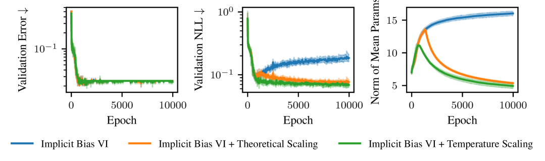
Figure S2: NLL overfitting in classification due to implicit bias of the mean parameters. As shown here for a two-hidden layer neural network on synthetic data, when training with vanilla SGD the mean parameters diverge to infinity $\lVert{\bm{\mu}}_{t}\rVert_{2}\approx\mathcal{O}\left(\log(t)\right)$ (right) and thus the classifier will eventually overfit in terms of negative log-likelihood (left and middle). Rescaling the GD iterates as in Theorem 2 or using temperature scaling [69] avoids overfitting.

This bias of the mean parameters towards the max-margin solution does not impact the train loss or validation error, but leads to overfitting in terms of validation NLL (see Figure S2) as long as there is at least one misclassified datapoint ${\bm{x}}$, since then the (average) validation NLL is given by

$$\bar{\ell}({\bm{\theta}}_{t}^{\textnormal{GD}}) =\textstyle\operatorname{\mathbb{E}}_{q_{{\bm{\theta}}_{t}^{\textnormal{GD}}}({\bm{w}})}\mathopen{}\left(\exp(-y{\bm{x}}^{\mathsf{T}}{\bm{w}})\right)=\exp({\bm{x}}^{\mathsf{T}}{\bm{\mu}}_{t}^{\textnormal{GD}}+\frac{1}{2}{\bm{x}}^{\mathsf{T}}{\bm{S}}_{t}^{\textnormal{GD}}({\bm{S}}_{t}^{\textnormal{GD}})^{\mathsf{T}}{\bm{x}})$$ (S100)

$$\approx\textstyle\exp(\log(t){\bm{x}}^{\mathsf{T}}\hat{{\bm{\mu}}}+\frac{1}{2}{\bm{x}}^{\mathsf{T}}{\bm{S}}_{t}^{\textnormal{GD}}({\bm{S}}_{t}^{\textnormal{GD}})^{\mathsf{T}}{\bm{x}})\to\infty\quad\text{as}\quad t\to\infty.$$

However, by rescaling the mean parameters as we do in Theorem 2, this can be prevented as Figure S2 (middle panel) illustrates for a two-hidden layer neural network on synthetic data. Such overfitting in terms of NLL has been studied extensively empirically with the perhaps most common remedy being Temperature Scaling (TS) [69]. As we show empirically in Figure S2, instead of using the theoretical rescaling, using temperature scaling performs very well, especially in the non-asymptotic regime, which is why we also adopt it for our experiments in Section 5.

The aforementioned divergence of the mean parameters to infinity also explains the need for the projection of the prior mean parameters in Equation 10, since any bias from the initialization vanishes in the limit of infinite training. At first glance the additional projection seems computationally prohibitive for anything but a zero mean prior, but close inspection of the implicit bias of the covariance parameters ${\bm{S}}$ in Theorem 2 shows that at convergence

$$\forall n:\operatorname{Var}_{q_{{\bm{\theta}}}}\mathopen{}\left(f_{\bm{w}}({\bm{x}}_{n})\right)={\bm{x}}_{n}^{\mathsf{T}}{\bm{S}}{\bm{S}}^{\mathsf{T}}{\bm{x}}_{n}=0\implies\operatorname{range}({\bm{S}})\subset\operatorname{null}({\bm{X}})$$ (S101)

Meaning we can approximate a basis of the null space of the training data by computing a QR decomposition of the covariance factor in $\mathcal{O}\left(PR^{2}\right)$ once at the end of training. For $R=P$ the inclusion becomes an equality and the projection can be computed exactly.

S2 Parametrization, Feature Learning and Hyperparameter Transfer

Notation

For this section we need a more detailed neural network notation. Denote an $L$-hidden layer, width-$0pt$ feedforward neural network by $f({\bm{x}})\in\mathbb{R}^{D}_{\text{out}}$, with inputs ${\bm{x}}\in\mathbb{R}^{D_{\text{in}}}$, weights ${\bm{W}}^{(l)}$, pre-activations ${\bm{h}}^{(l)}({\bm{x}})\in\mathbb{R}^{0pt^{(l)}}$, and post-activations (or “features”) ${\bm{g}}^{(l)}({\bm{x}})\in\mathbb{R}^{0pt^{(l)}}$. That is, ${\bm{h}}^{(1)}({\bm{x}})={\bm{W}}^{(1)}{\bm{x}}$ and, for $l\in 1,\dotsc,L-1$,

$${\bm{g}}^{(l)}({\bm{x}})={\phi\left({{\bm{h}}^{(l)}({\bm{x}})}\right)},\ {\bm{h}}^{(l+1)}({\bm{x}})={\bm{W}}^{(l+1)}{\bm{g}}^{(l)}({\bm{x}}),$$

and the network output is given by $f({\bm{x}})={\bm{W}}^{(L+1)}{\bm{g}}^{(L)}({\bm{x}})$, where ${\phi\left({\bullet}\right)}$ is an activation function.

For convenience, we may abuse notation and write ${\bm{h}}^{(0)}({\bm{x}})={\bm{x}}$ and ${\bm{h}}^{(L+1)}({\bm{x}})=f({\bm{x}})$. Throughout we use $\bullet^{(l)}$ to indicate the layer, subscript $\bullet_{t}$ to indicate the training time (i.e., epoch), $\Delta\bullet_{t}=\bullet_{t}-\bullet_{0}$ to indicate the change since initialization, and $[{\bullet}]_{i}$, $[{\bullet}]_{ij}$ to indicate the component within a vector or matrix.

S2.1 Definitions of Stability and Feature Learning

The following definitions extend those of [36] to the variational setting.

Definition S1 (bc scaling)

In layer $l$, the variational parameters are initialized as

$$[{{\bm{\mu}}_{0}^{(l)}}]_{i}\sim{\operatorname{\mathcal{N}}\mathopen{}\left(0,0pt^{-2b^{(l)}}\right)},\quad[{{\bm{S}}_{0}^{(l)}}]_{ij}\sim{\operatorname{\mathcal{N}}\mathopen{}\left(0,0pt^{-2\tilde{b}^{(l)}}\right)}$$

and the learning rates for the mean and covariance parameters, respectively, are set to

$$\eta^{(l)}=\eta 0pt^{-c^{(l)}},\tilde{\eta}^{(l)}=\eta 0pt^{-\tilde{c}^{(l)}}.$$

The hyperparameter $\eta$ represents a global learning rate that can be tuned, as for example in the hyperparameter transfer experiment from Section 3.4.

For the next two definitions, let $m_{r}\left(X\right)=\operatorname{\mathbb{E}}_{{\bm{z}}}\mathopen{}\left((X-\operatorname{\mathbb{E}}_{{\bm{z}}}\mathopen{}\left(X\right))^{r}\right)$ denote the $r$th central moment moment of a random variable $X$ with respect to ${\bm{z}}$, which represents all reparameterization noise in the random variable $X$. All Landau notation in Section S2 refers to asymptotic behavior in width $0pt$ in probability over reparameterization noise ${\bm{z}}$. We say that a vector sequence $\{{\bm{v}}_{0}pt\}_{0pt=1}^{\infty}$, where each ${\bm{v}}_{0}pt\in\mathbb{R}^{0}pt$, is $\mathcal{O}\left(0pt^{-a}\right)$ if the scalar sequence $\{\sqrt{\tfrac{1}{0pt}\lVert{\bm{v}}_{0}pt\rVert^{2}}\}_{0pt=1}^{\infty}=\{\text{RMSE}({\bm{v}}_{0}pt)\}_{0pt=1}^{\infty}$ is $\mathcal{O}\left(0pt^{-a}\right)$.

Definition S2 (Stability of Moment $r$)

A neural network is stable in moment $r$, if all of the following hold for all ${\bm{x}}$ and $l\in\{1,\dotsc,L\}$.

1. At initialization ($t=0$):

   1. The pre- and post-activations are $\Theta(1)$:

      $$m_{r}({\bm{h}}_{0}^{(l)}({\bm{x}})),m_{r}({\bm{g}}_{0}^{(l)}({\bm{x}}))=\Theta(1)$$

   2. The function is $\mathcal{O}\left(1\right)$:

      $$m_{r}(f_{0}({\bm{x}}))=\mathcal{O}\left(1\right)$$

2. At any point during training $t>0$:

   1. The change from initialization in the pre- and post-activations are $\mathcal{O}\left(1\right)$:

      $$\Delta m_{r}({\bm{h}}_{t}^{(l)}({\bm{x}})),\Delta m_{r}({\bm{g}}_{t}^{(l)}({\bm{x}}))=\mathcal{O}\left(1\right)$$

   2. The function is $\mathcal{O}\left(1\right)$:

      $$m_{r}(f_{t}({\bm{x}}))=\mathcal{O}\left(1\right)$$

Definition S3 (Feature Learning of Moment $r$)

Feature learning occurs in moment $r$ in layer $l$ if, for any $t>0$, the change from initialization is $\Omega(1)$:

$$\Delta m_{r}\left({\bm{g}}_{t}^{(l)}({\bm{x}})\right)=\Omega(1).$$

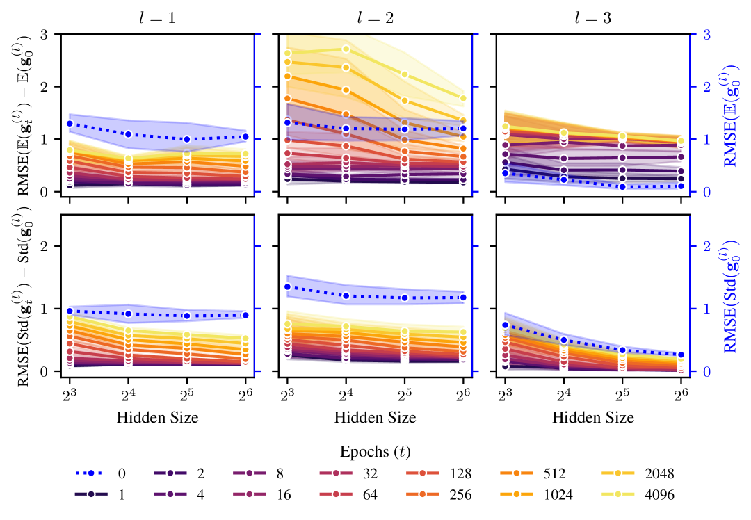
Figure S6: Variational MLP, Maximal Update Parametrization. RMSE of the change in the hidden units and, in blue, their initial values. Shaded region represents 95% confidence interval over 5 random initializations. The variational MLP is trained under $\mu$P with a full rank covariance in each layer.

As we will see later, Figure S5 and Figure S6 investigate feature learning for the first two moments.

S2.2 Initialization Scaling for a Linear Network

In this section we illustrate how the initialization scaling $\{(b^{(l)},\tilde{b}^{(l)})\}$ can be chosen for stability. For simplicity, we consider a linear feedforward network of width $0pt$ evaluated on a single input ${\bm{x}}\in\mathbb{R}^{D}_{\text{in}}$. We assume a Gaussian variational family that factorizes across layers. This implies the hidden units evolve as ${\bm{h}}_{t}^{(l+1)}={\bm{W}}_{t}^{(l+1)}{\bm{h}}_{t}^{(l)}$ and the weights are linked to the variational parameters by $\operatorname{vec}({\bm{W}}_{t}^{(l)})={\bm{\mu}}_{t}^{(l)}+{\bm{S}}_{t}^{(l)}{\bm{z}}$.

Therefore, the mean and variance of the $i$th component hidden units in layer $l\in\{1,\dotsc,L+1\}$, where $i\in 1\dotsc,0pt^{(l)}$, are given by

$$\operatorname{\mathbb{E}}_{z}\mathopen{}\left([{{\bm{h}}_{t}^{(l)}}]_{i}\right) =[{{\bm{\mu}}_{t}^{(l)}}]_{I}^{{\mathsf{T}}}\operatorname{\mathbb{E}}_{z}\mathopen{}\left({\bm{h}}_{t}^{(l-1)}\right)$$

$$\operatorname{Var}_{z}\mathopen{}\left([{{\bm{h}}_{t}^{(l)}}]_{i}\right) =[{{\bm{\mu}}_{t}^{(l)}}]_{I}^{{\mathsf{T}}}{\bm{C}}_{t}^{(l-1)}[{{\bm{\mu}}^{(l)}}]_{I}+\operatorname{tr}([{{\bm{S}}_{t}^{(l)}}]_{I,:}^{\mathsf{T}}{\bm{A}}_{t}^{(l-1)}[{{\bm{S}}_{t}^{(l)}}]_{I,:}),$$

where $I=\{iD^{(l-1)},\dotsc,(i+1)0pt^{(l-1)}\}$ and the second moment of and covariance of layer-$l$ hidden units are denoted by

$${\bm{A}}_{t}^{(l)} =\operatorname{\mathbb{E}}_{z}\mathopen{}\left({\bm{h}}_{t}^{(l)}{\bm{h}}_{t}^{(^{(l)}){{\mathsf{T}}}}\right)$$

$${\bm{C}}_{t}^{(l)} ={\bm{A}}_{t}^{(l)}-\operatorname{\mathbb{E}}_{z}\mathopen{}\left({\bm{h}}_{t}^{(l)}\right)\operatorname{\mathbb{E}}_{z}\mathopen{}\left({\bm{h}}_{t}^{(l)}\right)^{{\mathsf{T}}}.$$

Mean

We start with the mean of the hidden units, which conveniently depends only on the mean variational parameters and the previous layer hidden units.

$$\operatorname{\mathbb{E}}_{z}\mathopen{}\left([{{\bm{h}}_{0}^{(l)}}]_{i}\right) =\sum_{j=1}^{0pt^{(l-1)}}[{{\bm{\mu}}_{0}^{(l)}}]_{I_{j}}\operatorname{\mathbb{E}}_{z}\mathopen{}\left([{{\bm{h}}_{0}^{(l-1)}}]_{j}\right)$$

$$=\mathcal{O}\left(\sqrt{0pt^{(l-1)}}\cdot 0pt^{-b^{(l)}}\cdot 1\right)$$

$$=\begin{cases}\mathcal{O}\left(0pt^{-b^{(1)}}\right)&l=1\\ \mathcal{O}\left(0pt^{-(b^{(l)}-\tfrac{1}{2})}\right)&l\in\{2,\dotsc,L+1\}\end{cases}.$$

Therefore, we require $b^{(1)}\geq 0$ and $b^{(l)}\geq\tfrac{1}{2}$ for $l\in\{2,\dotsc,L+1\}$.

Variance

Next we examine the variance of hidden units. Consider the first term, which represents the contribution of the mean parameters.

$$[{{\bm{\mu}}_{0}^{(l)}}]_{I}^{{\mathsf{T}}}{\bm{C}}_{0}^{(l-1)}[{{\bm{\mu}}^{(l)}}]_{I} =\sum_{j=1}^{0pt^{(l-1)}}[{{\bm{\mu}}_{0}^{(l)}}]_{I_{j}}^{2}[{{\bm{C}}_{0}^{(l-1)}}]_{j,j}+\sum_{j\neq j^{\prime}}^{0pt^{(l-1)}}[{{\bm{\mu}}_{0}^{(l)}}]_{I_{j}}[{{\bm{C}}_{0}^{(l-1)}}]_{j,j^{\prime}}[{{\bm{\mu}}_{0}^{(l)}}]_{I_{j^{\prime}}}$$

$$=\mathcal{O}\left(0pt^{(l-1)}\cdot 0pt^{-2b^{(l)}}\cdot 1\right)+\mathcal{O}\left(\sqrt{0pt^{(l-1)}(0pt^{(l-1)}-1)}\cdot 0pt^{-b^{(l)}}\cdot 1\cdot 0pt^{-b^{(l)}}\right)$$

$$=\mathcal{O}\left(0pt^{(l-1)}\cdot 0pt^{-2b^{(l)}}\right)$$

$$=\begin{cases}\mathcal{O}\left(0pt^{-2b^{(1)}}\right)&l=1\\ \mathcal{O}\left(0pt^{-(2b^{(l)}-1)}\right)&l\in l\in\{2,\dotsc,L+1\}.\end{cases}$$

Therefore, we require $b^{(1)}\geq 0$ and $b^{(l)}\geq\tfrac{1}{2}$ for $l\in\{2,\dotsc,L+1\}$. Notice these are the same requirements as above for the mean of the hidden units. We summarize the scaling for the mean parameters as

$$\boxed{b^{(l)}\geq\begin{cases}0&l=1\\ \tfrac{1}{2}&l\in\{2,\dotsc,L+1\}.\end{cases}}$$ (S102)

Now consider the second term in the variance of the hidden units. Assume the rank scales with the input and output dimension of a layer as $R^{(l)}=(0pt^{(l-1)}0pt^{(l)})^{p^{(l)}}$, where $p^{(l)}\in[0,1]$.

$$\operatorname{tr}([{{\bm{S}}_{0}^{(l)}}]_{I,:}^{\mathsf{T}}{\bm{A}}_{0}^{(l-1)}[{{\bm{S}}_{0}^{(l)}}]_{I,:}) =\sum_{r=1}^{R^{(l)}}[{{\bm{S}}_{0}^{(l)}}]_{I,r}^{\mathsf{T}}{\bm{A}}_{0}^{(l-1)}[{{\bm{S}}_{0}^{(l)}}]_{I,r}$$

$$=\sum_{r=1}^{R^{(l)}}\left(\sum_{j=1}^{0pt^{(l-1)}}[{{\bm{S}}_{0}^{(l)}}]_{I_{j},r}^{2}[{{\bm{A}}_{0}^{(l-1)}}]_{j,j}+\sum_{j\neq j^{\prime}}^{0pt^{(l-1)}}[{{\bm{S}}_{0}^{(l)}}]_{I_{j},r}[{{\bm{A}}_{0}^{(l-1)}}]_{j,j^{\prime}}[{{\bm{S}}_{0}^{(l)}}]_{I_{j^{\prime}},r}\right)$$

$$=\mathcal{O}\left(R^{(l)}0pt^{(l-1)}\cdot 0pt^{-2\tilde{b}^{(l)}}\cdot 1\right)+\mathcal{O}\left(\sqrt{R^{(l)}0pt^{(l-1)}(0pt^{(l-1)}-1)}\cdot 0pt^{-\tilde{b}^{(l)}}\cdot 1\cdot 0pt^{-\tilde{b}^{(l)}}\right)$$

$$=\mathcal{O}\left(R^{(l)}0pt^{(l-1)}0pt^{-2\tilde{b}^{(l)}}\right)$$

$$=\begin{cases}\mathcal{O}\left(0pt^{-(2\tilde{b}^{(1)}-p^{(1)})}\right)&l=1\\ \mathcal{O}\left(0pt^{-(2\tilde{b}^{(l)}-1-2p^{(l)})}\right)&l\in\{2,\dotsc,L\}\\ \mathcal{O}\left(0pt^{-(2\tilde{b}^{(L+1)}-1-p^{(L+1)})}\right)&l=L+1.\end{cases}$$

Therefore we require $\tilde{b}^{(0)}\geq\tfrac{p^{(1)}missing}{2}$, $\tilde{b}^{(l)}\geq\tfrac{1}{2}+p^{(l)}$ for $l\in\{2,\dotsc,L\}$, and $\tilde{b}^{(L+1)}\geq\tfrac{1}{2}+\tfrac{p^{(L+1)}missing}{2}$. Notice we can write these conditions in terms of the mean scaling as

$$\boxed{\tilde{b}^{(l)}\geq b^{(l)}+\begin{cases}\tfrac{p^{(l)}missing}{2}&l=1\\ p^{(l)}&l\in\{2,\dotsc,L\}\\ \tfrac{p^{(l)}missing}{2}&l=L+1.\end{cases}}$$ (S103)

S2.3 Proposed Scaling

The previous section derives the necessary conditions for stability at initialization. Recall from Section 3.4 that we propose scaling the contribution of the covariance parameters to the forward pass, i.e. the ${\bm{S}}{\bm{z}}$ term, by $R^{-1/2}$ since each element in the term is a sum over $R$ random variables, where $R$ is the rank of ${\bm{S}}$. In the more detailed notation of this section, the proposed scaling implies the forward pass in a linear layer is given by

$$[{{\bm{h}}^{(l)}_{t}}]_{i}=[{{\bm{W}}_{t}}]_{:,i}{\bm{h}}^{(l-1)}_{t}=\left([{{\bm{\mu}}^{(l)}_{t}}]_{I}+R^{-1/2}[{{\bm{S}}^{(l)}_{t}}]_{I}{\bm{z}}^{(l)}\right){\bm{h}}^{(l-1)}_{t}.$$ (S104)

In practice, rather than scaling $[{{\bm{S}}^{(l)}_{t}}]_{I}{\bm{z}}^{(l)}$ by $R^{-1/2}$ in the forward pass, we apply Lemma J.1 from [34] to instead scale the initialization by $R^{-1/2}$ and, in SGD, the learning rate by $R^{-1}$. Scaling by the rank allows treating the mean and covariance parameters as if they were weights parameterized by $\mu$P in a non-probabilistic network, inheriting any scaling that has already been derived for that architecture.

From Table 3 of [34], we therefore scale the mean parameters as

$$b^{(l)}=\begin{cases}0&l=1\\ 1/2&l\in\{2,\dotsc,L\}\\ 1&l=L+1\end{cases}\quad\text{and}\quad c^{(l)}=\begin{cases}-1&l=1\\ 0&l\in\{2,\dotsc,L\}\\ 1&l=L+1.\end{cases}$$ (S105)

Assuming $R^{(l)}=(0pt^{(l-1)}0pt^{(l)})^{p^{(l)}}$ as before, where $p^{(l)}\in[0,1]$, we the scale the covariance parameters as

$$\tilde{b}^{(l)}=b^{(l)}+\begin{cases}\tfrac{p^{(l)}missing}{2}&l=1\\ p^{(l)}&l\in\{2,\dotsc,L\}\\ \tfrac{p^{(l)}missing}{2}&l=L+1\end{cases}\quad\text{and}\quad\tilde{c}^{(l)}=c^{(l)}+\begin{cases}p^{(l)}&l=1\\ 2p^{(l)}&l\in\{2,\dotsc,L\}\\ p^{(l)}&l=L+1.\end{cases}$$ (S106)

By comparing to Equations S102 and S103, we see the mean and covariance parameters in all but the output layer are initialized as large as possible while still maintaining stability. The output layer parameters scale to zero faster, since, as in $\mu$P for the weights of non-probabilistic networks, we set $b^{(L+1)}$ to $1$ instead of $1/2$.

Note that in Section S2.2 we did not consider input and output dimensions that scaled with the width $0pt$ for simplicity. For our experiments, we take the exact $\mu$P initialization and learning rate scaling from Yang et al. [34] — which includes, for example, a $1/\texttt{fan\_in}$ scaling in the input layer — for the means and then make the rank adjustment for the covariance parameters as described above.

We investigate the proposed scaling in Figures S4 and S5. We train two-hidden-layer ($L=2$) MLPs of hidden sizes 8, 16, 32, and 64 on a single observation $(x,y)=(1,1)$ using a squared error loss. We use SGD with a learning rate of 0.05. For the variational networks, we assume a multivariate Gaussian variational family with a full rank covariance.

Figures S3 and S4 show the RMSE of the change in the hidden units from initialization, $\Delta{\bm{g}}_{t}^{(l)}(x)={\bm{g}}_{t}^{(l)}(x)-{\bm{g}}_{0}^{(l)}(x)$, as a function of the hidden size. The RMSE of the hidden units at initialization, ${\bm{g}}_{0}^{(l)}$ is also shown in blue. Each panel corresponds to a layer of the network, so the first two panels correspond to features ${\bm{g}}_{t}^{(1)}(x)$ and ${\bm{g}}_{t}^{(2)}(x)$, respectively, while the third panel corresponds to the output of the network, ${\bm{g}}_{t}^{(3)}(x)=f_{t}(x)$. The difference between the figures is the paramaterization. Figure S3 uses standard parameterization (SP) while Figure S4 uses maximal update parametrization ($\mu$P). We observe that (a) the features change more under $\mu$P than SP and (b) training is more stable across hidden sizes under $\mu$P than SP, especially for smaller networks.

Figures S5 and S6 show the analogous results for a variational network. The top row shows the change in the mean of the hidden units, while the bottom row shows the change in the standard deviation. As in the non-probabilistic case, we observe that (a) both the mean and standard deviation of the features change more under $\mu$P than SP and (b) training is more stable across hidden sizes under $\mu$P than SP, especially for smaller networks.

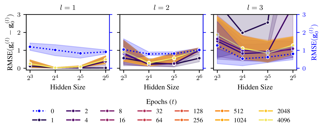
Figure S3: MLP, Standard Parameterization. RMSE of the change in the hidden units and, in blue, their initial values. Shaded region represents 95% confidence interval over 5 random initializations. The MLP is trained under SP.

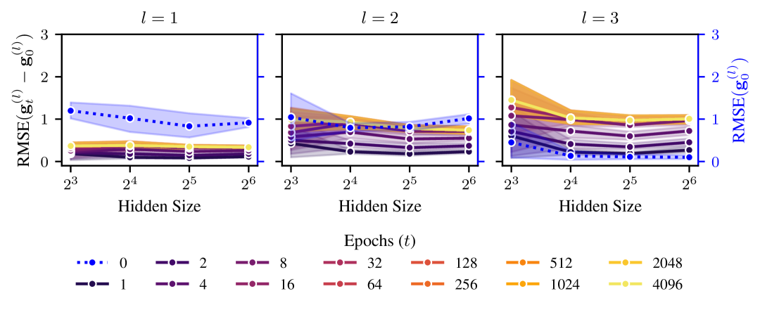
Figure S4: MLP, Maximal Update Parameterization. RMSE of the change in the hidden units and, in blue, their initial values. Shaded region represents 95% confidence interval over 5 random initializations. The MLP is trained under $\mu$P.

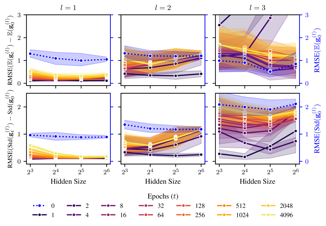
Figure S5: Variational MLP, Standard Parameterization. RMSE of the change in the hidden units and, in blue, their initial values. Shaded region represents 95% confidence interval over 5 random initializations. The variational MLP is trained under SP with a full rank covariance in each layer.

S2.4 Details on Hyperparameter Transfer Experiment

As discussed in Section 3.4 we train two-hidden-layer MLPs of width 128, 256, 512, 1024, and 2048 on CIFAR-10. For comparability to Figure 3 in Tensor Programs V [34] we use the same hyperparameters but applied to the mean parameters. For the input layer, we scale the mean parameters at initialization by a factor of 16 and in the forward pass by a factor of 1/16. For the output layer, we scale the mean parameters by 0.0 at initialization and by 32.0 in the forward pass. We use 20 epochs, batch size 64, and a grid of global learning rates ranging from $2^{-8}$ to $2^{0}$ with cosine annealing during training. For the grid search results shown in the right panel of Figure 3, we use validation NLL for model selection and then evaluate the relative test error compared to the best performing model for that width across parameterizations and learning rates.

S3 Experiments

This section outlines in more detail the experimental setup, including datasets (Section S3.1.1), metrics (Section S3.1.2), architectures, the training setup and method details (Section S3.3.1). It also contains additional experiments to the ones in the main paper (Sections S3.2, S3.3.2 and S3.3.3).

S3.1 Setup and Details

In all of our experiments we used the following datasets and metrics.

S3.1.1 Datasets

Table S1: Benchmark datasets used in our experiments. All corrupted datasets are only intended for evaluation and thus only have test sets consisting of 15 different corruptions of the original test set.

Dataset	$N$	${N_{\mathrm{test}}}$	$D_{\text{in}}$	$C$	Train / Validation Split
MNIST [70]	60 000	10 000	28 $\times$ 28	10	(0.9, 0.1)
CIFAR-10 [80]	50 000	10 000	3 $\times$ 32 $\times$ 32	10	(0.9, 0.1)
CIFAR-100 [80]	50 000	10 000	3 $\times$ 32 $\times$ 32	100	(0.9, 0.1)
TinyImageNet [81]	100 000	10 000	3 $\times$ 64 $\times$ 64	200	(0.9, 0.1)
MNIST-C [72]	-	150 000	28 $\times$ 28	10	-
CIFAR-10-C [73]	-	150 000	3 $\times$ 32 $\times$ 32	10	-
CIFAR-100-C [73]	-	150 000	3 $\times$ 32 $\times$ 32	100	-
TinyImageNet-C [73]	-	150 000	3 $\times$ 64 $\times$ 64	200	-

S3.1.2 Metrics

Accuracy

The (top-k) accuracy is defined as

$$\operatorname{Accuracy}_{k}({\bm{y}},\hat{{\bm{y}}})=\frac{1}{{N_{\mathrm{test}}}}\sum_{n=1}^{{N_{\mathrm{test}}}}1_{(y_{n}\in\hat{y}_{n}^{1:k})}.$$ (S107)

Negative Log-Likelihood (NLL)

The (normalized) negative log likelihood for classification is given by

$$\operatorname{NLL}({\bm{y}},\hat{{\bm{y}}})=-\frac{1}{{N_{\mathrm{test}}}}\sum_{n=1}^{{N_{\mathrm{test}}}}\log\hat{{\bm{p}}}_{\hat{y}_{n}},$$ (S108)

where $\hat{{\bm{p}}}_{\hat{y}_{n}}$ is the probability a model assigns to the predicted class $\hat{y}_{n}$.

Expected Calibration Error (ECE)

The expected calibration error measures how well a model is calibrated, i.e. how closely the predicted class probability matches the accuracy of the model. Assume the predicted probabilities of the model on the test set are binned into a given binning of the unit interval. Compute the accuracy $a_{j}$ and average predicted probability $\hat{p}_{j}$ of each bin, then the expected calibration error is given by

$$\operatorname{ECE}=\sum_{j=1}^{J}b_{j}\lvert a_{j}-\hat{p}_{j}\rvert,$$ (S109)

where $b_{j}$ is the fraction of datapoints in bin $j\in\{1,\dots,J\}$.

S3.2 Time and Memory-Efficient Training

To keep the time and memory overhead low during training, we would like to draw as few samples of the parameters as possible to evaluate the training objective $\bar{\ell}({\bm{\theta}})$. Drawing $M$ parameter samples for the loss increases the time and memory overhead of a forward and backward pass $M$ times (disregarding parallelism). Therefore it is paramount for efficiency to use as few parameter samples as possible, ideally $M=1$.

When drawing fewer samples from the variational distribution, the variance in the training loss and gradients increases. In practice this means one has to potentially choose a smaller learning rate to still achieve good performance. This is analogous to the previously observed linear relationship $N_{b}\propto\eta$ between the optimal batch size $N_{b}$ and learning rate $\eta$ [[, e.g.,]]Goyal2018AccurateLarge,Smith2018BayesianPerspective,Smith2018DontDecay. Figure S7 shows this relationship between the number of parameter samples used for training and the learning rate on MNIST for a two-hidden layer MLP of width 128.

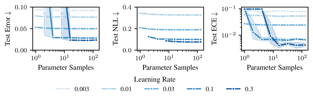
Figure S7: Generalization versus number of parameter samples. For a fixed number of epochs and batch size, fewer samples require a smaller learning rate. For a fixed learning rate, generalization performance quickly plateaus with more parameter samples.

As Figure S8 shows, when using momentum, generalization performance tends to increase, but only if either the number of samples is increased, or the learning rate is decreased accordingly. A similar relationship between noise in the objective and the use of momentum has previously been observed by [29], which propose and empirically verify a scaling law for the optimal batch size $N_{b}\propto\frac{\eta}{1-\gamma}$ as a function of the momentum parameter $\gamma>0$.

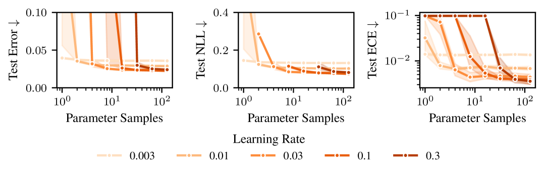
Figure S8: Generalization versus number of parameter samples when using momentum. Using momentum improves generalization performance, but when using fewer parameter samples, a smaller learning rate is necessary than for vanilla SGD as predicted by Equation 6.

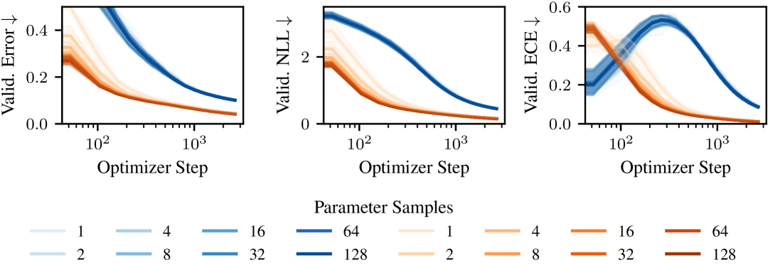
Figure S9: Validation error during training for different numbers of parameter samples. The difference in generalization error between different number of parameter samples vanishes with more optimization steps both for SGD ( ) and when using momentum ( ), if the learning rate is sufficiently small (in this example $\eta=0.003$).

S3.3 In- and Out-of-distribution Generalization

This section recounts details of the methods we benchmark in Section 5, how they are trained and additional experimental results.

S3.3.1 Architectures, Training, and Methods

Architectures

We use convolutional architectures for all experiments in Section 5. For MNIST, we use a standard LeNet-5 [70] with ReLU activations. For CIFAR-10, CIFAR-100 and TinyImageNet we use a ResNet-34 [71] where the first layer is a 2D convolution with kernel_size=3, stride=1 and padding=1 to account for the image resolution of CIFAR and TinyImageNet and the normalization layers are GroupNorm layers. We use pretrained weights from ImageNet for all but the first and last layer of the ResNets from torchvision [82] and fully finetune all parameters during training.

Training

We train all models using SGD with momentum ($\gamma=0.9)$ with batch size $N_{b}=128$ and learning rate $\eta=0.005$ for $200$ epochs. We do not use a learning rate scheduler since we found that neither cosine annealing nor learning rate warm-up improved the results.

Temperature Scaling [69]

For temperature scaling we optimize the scalar temperature parameter in the last layer on the validation set via the L-BFGS implementation in torch with an initial learning rate $\eta=0.1$, a maximum number of 100 iterations per optimization step and history_size=100.

Laplace Approximation (Last-Layer, GS + ML) [52]

As recommended by [52] we use a post-hoc KFAC last-layer Laplace approximation with a GGN approximation to the Hessian. We tune the hyperparameters post-hoc using type-II maximum likelihood (ML). As an alternative we also do a grid search (GS) for the prior scale, which we found to be somewhat more robust in our experiments. Finally, we compute the predictive using an (extended) probit approximation. Our implementation of the Laplace approximation is a thin wrapper of laplace [52] and we use its default hyperparameters throughout.

Weight-space VI (Mean-field) [37, 38]

For variational inference, we used a mean-field variational family and trained via an ELBO objective with a weighting of the Kullback-Leibler regularization term to the prior. We chose a unit-variance Gaussian prior with mean that was set to the pretrained weights, except for the in- and output layer which had zero mean. We found that using a KL weight and more than a single sample (here $M=8$) was necessary to achieve competitive performance. The KL weight was chosen to be inversely proportional to the number of parameters of the model, for which we observed better performance than a KL weight that was independent of the architecture. At test time we compute the predictive by averaging logits using $32$ samples.

Implicit Bias VI [ours]

For all architectures in Section 5 we use a Gaussian in- and output layer with a low-rank covariance ($R=10,20$). We train with a single parameter sample $M=1$ throughout and do temperature scaling at the end of training on the validation set with the same settings as when just performing temperature scaling. We do temperature scaling in classification due to the specific form of the implicit bias in classification as described in Section S1.3. Since IBVI trains by optimizing a minibatch approximation of the expected negative log-likelihood (an average over log-probabilities with respect to parameter samples), we also average log-probabilities at test-time to compute the predictive distribution over class probabilities. Although we did not see a significant difference between averaging log-probabilities, probabilities or logits. Like for WSVI we use $32$ samples at test time.

Deep Ensembles [55]

We use five ensemble members initialized and trained independently. We compute the predictive by averaging the predicted probabilities of the ensemble members in line with standard practice [55]. We did not see a significant difference in performance between averaging logits or averaging class probabilities.

S3.3.2 In-Distribution Generalization and Uncertainty Quantification

The full results from the in-distribution generalization experiment in Section 5 can be found in Figure S10. The same experiment but done in the Maximal Update parametrization is depicted in Figure S11. When finetuning a pretrained model, we found that on some datasets (CIFAR-100, TinyImageNet) $\mu$P resulted in somewhat lower performance, contrary to the results in Section 3.4, where we trained from scratch. This suggests that, when pretraining, there may be a modification to the parametrization that could improve generalization.

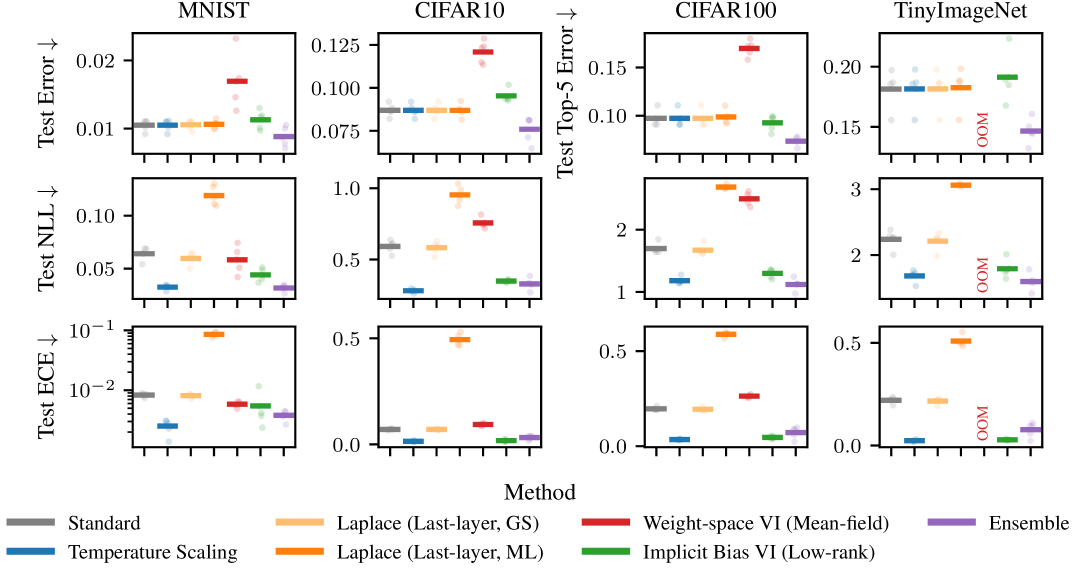
Figure S10: In-distribution generalization and uncertainty quantification (Standard parametrization).

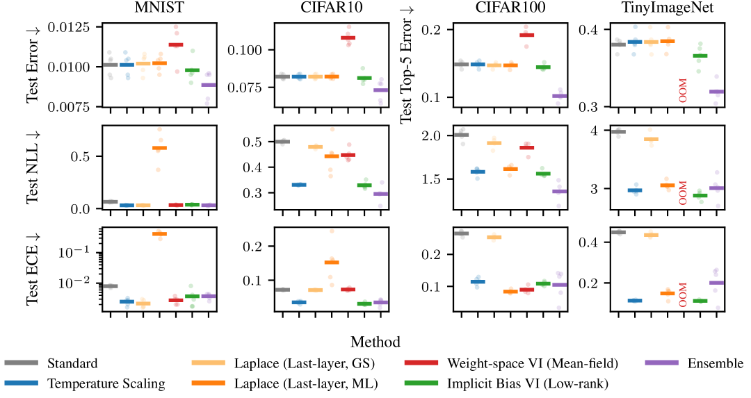
Figure S11: In-distribution generalization and uncertainty quantification (Maximal Update parametrization).

S3.3.3 Robustness to Input Corruptions

Besides the benchmark in Figure S11, we also evaluated the models trained using the Maximal Update parametrization on the corrupted datasets. The results can be found in Figure S12.

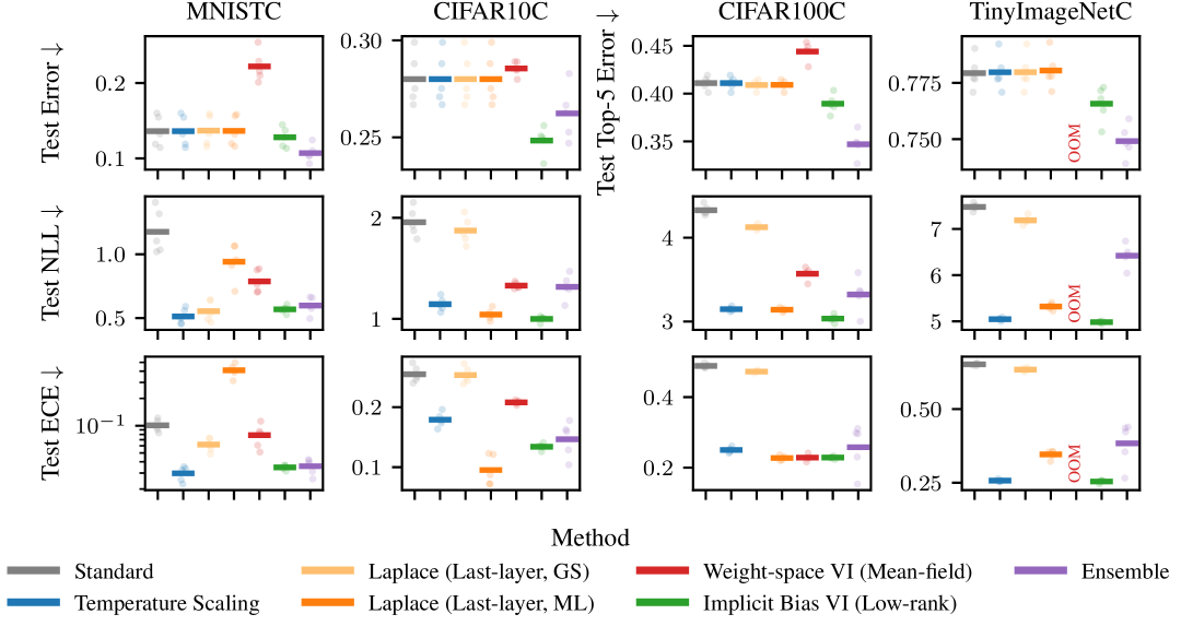
Figure S12: Generalization on robustness benchmark problems (Maximal Update parametrization).

[supplementary]

References

- [1] Micah Goldblum, Marc Finzi, Keefer Rowan and Andrew Gordon Wilson “The No Free Lunch Theorem, Kolmogorov Complexity, and the Role of Inductive Biases in Machine Learning” In International Conference on Machine Learning (ICML), 2024 DOI: 10.48550/arXiv.2304.05366
- [2] Mor Shpigel Nacson, Rotem Mulayoff, Greg Ongie, Tomer Michaeli and Daniel Soudry “The Implicit Bias of Minima Stability in Multivariate Shallow ReLU Networks” In International Conference on Learning Representations (ICLR), 2023 DOI: 10.48550/arXiv.2306.17499
- [3] Rotem Mulayoff, Tomer Michaeli and Daniel Soudry “The Implicit Bias of Minima Stability: A View from Function Space” In Advances in Neural Information Processing Systems (NeurIPS), 2021 URL: https://proceedings.neurips.cc/paper/2021/hash/944a5ae3483ed5c1e10bbccb7942a279-Abstract.html
- [4] Daniel Soudry, Elad Hoffer, Mor Shpigel Nacson, Suriya Gunasekar and Nathan Srebro “The Implicit Bias of Gradient Descent on Separable Data” In Journal of Machine Learning Research (JMLR), 2018 DOI: 10.48550/arXiv.1710.10345
- [5] Suriya Gunasekar, Jason Lee, Daniel Soudry and Nathan Srebro “Characterizing Implicit Bias in Terms of Optimization Geometry” In International Conference on Machine Learning (ICML), 2018 DOI: 10.48550/arXiv.1802.08246
- [6] Mor Shpigel Nacson, Jason D. Lee, Suriya Gunasekar, Pedro H.. Savarese, Nathan Srebro and Daniel Soudry “Convergence of Gradient Descent on Separable Data” In International Conference on Artificial Intelligence and Statistics (AISTATS), 2019 DOI: 10.48550/arXiv.1803.01905
- [7] Mor Shpigel Nacson, Nathan Srebro and Daniel Soudry “Stochastic Gradient Descent on Separable Data: Exact Convergence with a Fixed Learning Rate” In International Conference on Artificial Intelligence and Statistics (AISTATS), 2019 DOI: 10.48550/arXiv.1806.01796
- [8] Bohan Wang, Qi Meng, Huishuai Zhang, Ruoyu Sun, Wei Chen, Zhi-Ming Ma and Tie-Yan Liu “Does Momentum Change the Implicit Regularization on Separable Data?” In Advances in Neural Information Processing Systems (NeurIPS), 2022
- [9] Hui Jin and Guido Montúfar “Implicit Bias of Gradient Descent for Mean Squared Error Regression with Two-Layer Wide Neural Networks” arXiv:2006.07356 [stat] arXiv, 2023 DOI: 10.48550/arXiv.2006.07356
- [10] Hrithik Ravi, Clayton Scott, Daniel Soudry and Yutong Wang “The Implicit Bias of Gradient Descent on Separable Multiclass Data” In Advances in Neural Information Processing Systems (NeurIPS), 2024 DOI: 10.48550/arXiv.2411.01350
- [11] Theodore Papamarkou, Maria Skoularidou, Konstantina Palla, Laurence Aitchison, Julyan Arbel, David Dunson, Maurizio Filippone, Vincent Fortuin, Philipp Hennig, José Miguel Hernández-Lobato, Aliaksandr Hubin, Alexander Immer, Theofanis Karaletsos, Mohammad Emtiyaz Khan, Agustinus Kristiadi, Yingzhen Li, Stephan Mandt, Christopher Nemeth, Michael A. Osborne, Tim G.. Rudner, David Rügamer, Yee Whye Teh, Max Welling, Andrew Gordon Wilson and Ruqi Zhang “Position: Bayesian Deep Learning is Needed in the Age of Large-Scale AI” In International Conference on Machine Learning (ICML), 2024 DOI: 10.48550/arXiv.2402.00809
- [12] Dustin Tran, Jeremiah Liu, Michael W. Dusenberry, Du Phan, Mark Collier, Jie Ren, Kehang Han, Zi Wang, Zelda Mariet, Huiyi Hu, Neil Band, Tim G.. Rudner, Karan Singhal, Zachary Nado, Joost van Amersfoort, Andreas Kirsch, Rodolphe Jenatton, Nithum Thain, Honglin Yuan, Kelly Buchanan, Kevin Murphy, D. Sculley, Yarin Gal, Zoubin Ghahramani, Jasper Snoek and Balaji Lakshminarayanan “Plex: Towards Reliability using Pretrained Large Model Extensions” arXiv, 2022 DOI: 10.48550/arXiv.2207.07411
- [13] Hippolyt Ritter, Aleksandar Botev and David Barber “Online Structured Laplace Approximations For Overcoming Catastrophic Forgetting” In Advances in Neural Information Processing Systems (NeurIPS), 2018 DOI: 10.48550/arXiv.1805.07810
- [14] Yucen Lily Li, Tim G.. Rudner and Andrew Gordon Wilson “A Study of Bayesian Neural Network Surrogates for Bayesian Optimization” In International Conference on Learning Representations (ICLR), 2024 DOI: 10.48550/arXiv.2305.20028
- [15] Vincent Fortuin “Priors in Bayesian Deep Learning: A Review” In International Statistical Review 90.3, 2022, pp. 563–591 DOI: 10.1111/insr.12502
- [16] Pavel Izmailov, Sharad Vikram, Matthew D. Hoffman and Andrew Gordon Wilson “What Are Bayesian Neural Network Posteriors Really Like?” In International Conference on Machine Learning (ICML), 2021 DOI: 10.48550/arXiv.2104.14421
- [17] Ben Adlam, Jasper Snoek and Samuel L. Smith “Cold Posteriors and Aleatoric Uncertainty” arXiv, 2020 DOI: 10.48550/arXiv.2008.00029
- [18] Tristan Cinquin, Alexander Immer, Max Horn and Vincent Fortuin “Pathologies in priors and inference for Bayesian transformers” In NeurIPS Bayesian Deep Learning Workshop, 2021 DOI: 10.48550/arXiv.2110.04020
- [19] Beau Coker, Wessel P. Bruinsma, David R. Burt, Weiwei Pan and Finale Doshi-Velez “Wide Mean-Field Bayesian Neural Networks Ignore the Data” In International Conference on Artificial Intelligence and Statistics (AISTATS), 2022 DOI: 10.48550/arXiv.2202.11670
- [20] Andrew Y.. Foong, David R. Burt, Yingzhen Li and Richard E. Turner “On the Expressiveness of Approximate Inference in Bayesian Neural Networks” In Advances in Neural Information Processing Systems (NeurIPS), 2020 DOI: 10.48550/arXiv.1909.00719
- [21] Chiyuan Zhang, Samy Bengio, Moritz Hardt, Benjamin Recht and Oriol Vinyals “Understanding deep learning requires rethinking generalization” In International Conference on Learning Representations (ICLR), 2017 DOI: 10.48550/arXiv.1611.03530
- [22] Gal Vardi “On the Implicit Bias in Deep-Learning Algorithms” In Commun. ACM 66.6, 2023, pp. 86–93 DOI: 10.1145/3571070
- [23] Bhavya Vasudeva, Puneesh Deora and Christos Thrampoulidis “Implicit Bias and Fast Convergence Rates for Self-attention”, 2024 DOI: 10.48550/arXiv.2402.05738
- [24] Arnold Zellner “Optimal Information Processing and Bayes’s Theorem” In The American Statistician 42.4, 1988, pp. 278–280 DOI: 10.2307/2685143
- [25] Pier Giovanni Bissiri, Chris Holmes and Stephen Walker “A General Framework for Updating Belief Distributions” In Journal of the Royal Statistical Society: Series B (Statistical Methodology) 78.5, 2016, pp. 1103–1130 DOI: 10.1111/rssb.12158
- [26] Jeremias Knoblauch, Jack Jewson and Theodoros Damoulas “An Optimization-centric View on Bayes’ Rule: Reviewing and Generalizing Variational Inference” In Journal of Machine Learning Research (JMLR) 23.132, 2022, pp. 1–109 URL: http://jmlr.org/papers/v23/19-1047.html
- [27] Veit D. Wild, Robert Hu and Dino Sejdinovic “Generalized Variational Inference in Function Spaces: Gaussian Measures meet Bayesian Deep Learning” In Advances in Neural Information Processing Systems (NeurIPS), 2022 DOI: 10.48550/arXiv.2205.06342
- [28] Priya Goyal, Piotr Dollár, Ross Girshick, Pieter Noordhuis, Lukasz Wesolowski, Aapo Kyrola, Andrew Tulloch, Yangqing Jia and Kaiming He “Accurate, Large Minibatch SGD: Training ImageNet in 1 Hour”, 2018 URL: http://arxiv.org/abs/1706.02677
- [29] Samuel L. Smith and Quoc V. Le “A Bayesian Perspective on Generalization and Stochastic Gradient Descent” In International Conference on Learning Representations (ICLR), 2018 DOI: 10.48550/arXiv.1710.06451
- [30] Samuel L. Smith, Pieter-Jan Kindermans, Chris Ying and Quoc V. Le “Don’t Decay the Learning Rate, Increase the Batch Size” In International Conference on Learning Representations (ICLR), 2018 DOI: 10.48550/arXiv.1711.00489
- [31] Sebastian Farquhar, Lewis Smith and Yarin Gal “Liberty or Depth: Deep Bayesian Neural Nets Do Not Need Complex Weight Posterior Approximations” In Advances in Neural Information Processing Systems (NeurIPS), 2020 DOI: 10.48550/arXiv.2002.03704
- [32] Mrinank Sharma, Sebastian Farquhar, Eric Nalisnick and Tom Rainforth “Do Bayesian Neural Networks Need To Be Fully Stochastic?” In International Conference on Artificial Intelligence and Statistics (AISTATS), 2023 DOI: 10.48550/arXiv.2211.06291
- [33] Boris Hanin and Mark Sellke “Approximating Continuous Functions by ReLU Nets of Minimal Width” arXiv:1710.11278 [stat] arXiv, 2018 DOI: 10.48550/arXiv.1710.11278
- [34] Greg Yang, Edward J. Hu, Igor Babuschkin, Szymon Sidor, Xiaodong Liu, David Farhi, Nick Ryder, Jakub Pachocki, Weizhu Chen and Jianfeng Gao “Tensor Programs V: Tuning Large Neural Networks via Zero-Shot Hyperparameter Transfer” In Advances in Neural Information Processing Systems (NeurIPS), 2021 DOI: 10.48550/arXiv.2203.03466
- [35] Anirban Bhattacharya, Antonio Linero and Chris J. Oates “Grand Challenges in Bayesian Computation” In Bulletin of the International Society for Bayesian Analysis (ISBA) 31.3, 2024 DOI: 10.48550/arXiv.2410.00496
- [36] Greg Yang and Edward J. Hu “Tensor Programs IV: Feature Learning in Infinite-Width Neural Networks” In International Conference on Machine Learning (ICML), 2021 DOI: 10.48550/arXiv.2011.14522
- [37] Alex Graves “Practical Variational Inference for Neural Networks” In Advances in Neural Information Processing Systems (NeurIPS), 2011 URL: https://papers.nips.cc/paper_files/paper/2011/hash/7eb3c8be3d411e8ebfab08eba5f49632-Abstract.html
- [38] Charles Blundell, Julien Cornebise, Koray Kavukcuoglu and Daan Wierstra “Weight Uncertainty in Neural Networks” In International Conference on Machine Learning (ICML), 2015 DOI: 10.48550/arXiv.1505.05424
- [39] Guodong Zhang, Shengyang Sun, David Duvenaud and Roger Grosse “Noisy Natural Gradient as Variational Inference” arXiv, 2018 DOI: 10.48550/arXiv.1712.02390
- [40] Minh-Ngoc Tran, Nghia Nguyen, David Nott and Robert Kohn “Bayesian Deep Net GLM and GLMM” arXiv, 2018 DOI: 10.48550/arXiv.1805.10157
- [41] Kazuki Osawa, Siddharth Swaroop, Anirudh Jain, Runa Eschenhagen, Richard E. Turner, Rio Yokota and Mohammad Emtiyaz Khan “Practical Deep Learning with Bayesian Principles” In Advances in Neural Information Processing Systems (NeurIPS), 2019 DOI: 10.48550/arXiv.1906.02506
- [42] Yuesong Shen, Nico Daheim, Bai Cong, Peter Nickl, Gian Maria Marconi, Clement Bazan, Rio Yokota, Iryna Gurevych, Daniel Cremers, Mohammad Emtiyaz Khan and Thomas Möllenhoff “Variational Learning is Effective for Large Deep Networks” In International Conference on Machine Learning (ICML), 2024 DOI: 10.48550/arXiv.2402.17641
- [43] Christos Louizos and Max Welling “Structured and Efficient Variational Deep Learning with Matrix Gaussian Posteriors” arXiv, 2016 DOI: 10.48550/arXiv.1603.04733
- [44] Aaron Mishkin, Frederik Kunstner, Didrik Nielsen, Mark Schmidt and Mohammad Emtiyaz Khan “SLANG: Fast Structured Covariance Approximations for Bayesian Deep Learning with Natural Gradient” arXiv, 2019 DOI: 10.48550/arXiv.1811.04504
- [45] James Harrison, John Willes and Jasper Snoek “Variational Bayesian Last Layers” In International Conference on Learning Representations (ICLR), 2024 DOI: 10.48550/arXiv.2404.11599
- [46] Jeremiah Zhe Liu, Zi Lin, Shreyas Padhy, Dustin Tran, Tania Bedrax-Weiss and Balaji Lakshminarayanan “Simple and Principled Uncertainty Estimation with Deterministic Deep Learning via Distance Awareness” arXiv, 2020 DOI: 10.48550/arXiv.2006.10108
- [47] David J.. MacKay “A Practical Bayesian Framework for Backpropagation Networks” In Neural Computation 4, 1992 DOI: 10.1162/neco.1992.4.3.448
- [48] Hippolyt Ritter, Aleksandar Botev and David Barber “A Scalable Laplace Approximation for Neural Networks” In International Conference on Learning Representations (ICLR), 2018
- [49] Mohammad Emtiyaz Khan, Alexander Immer, Ehsan Abedi and Maciej Korzepa “Approximate Inference Turns Deep Networks into Gaussian Processes” In Advances in Neural Information Processing Systems (NeurIPS), 2019 DOI: 10.48550/arXiv.1906.01930
- [50] Alexander Immer, Maciej Korzepa and Matthias Bauer “Improving predictions of Bayesian neural nets via local linearization” In International Conference on Artificial Intelligence and Statistics (AISTATS), 2021
- [51] Erik Daxberger, Eric Nalisnick, James Urquhart Allingham, Javier Antorán and José Miguel Hernández-Lobato “Bayesian Deep Learning via Subnetwork Inference” In International Conference on Machine Learning (ICML), 2021 DOI: 10.48550/arXiv.2010.14689
- [52] Erik Daxberger, Agustinus Kristiadi, Alexander Immer, Runa Eschenhagen, Matthias Bauer and Philipp Hennig “Laplace Redux – Effortless Bayesian Deep Learning” In Advances in Neural Information Processing Systems (NeurIPS), 2021 DOI: 10.48550/arXiv.2106.14806
- [53] Agustinus Kristiadi, Alexander Immer, Runa Eschenhagen and Vincent Fortuin “Promises and Pitfalls of the Linearized Laplace in Bayesian Optimization” In Advances in Approximate Bayesian Inference (AABI), 2023 DOI: 10.48550/arXiv.2304.08309
- [54] Tristan Cinquin, Marvin Pförtner, Vincent Fortuin, Philipp Hennig and Robert Bamler “FSP-Laplace: Function-Space Priors for the Laplace Approximation in Bayesian Deep Learning” In Advances in Neural Information Processing Systems (NeurIPS), 2024 DOI: 10.48550/arXiv.2407.13711
- [55] Balaji Lakshminarayanan, Alexander Pritzel and Charles Blundell “Simple and Scalable Predictive Uncertainty Estimation using Deep Ensembles” In Advances in Neural Information Processing Systems (NeurIPS), 2017 DOI: 10.48550/arXiv.1612.01474
- [56] Stanislav Fort, Huiyi Hu and Balaji Lakshminarayanan “Deep Ensembles: A Loss Landscape Perspective” arXiv, 2020 DOI: 10.48550/arXiv.1912.02757
- [57] Andrew Gordon Wilson and Pavel Izmailov “Bayesian Deep Learning and a Probabilistic Perspective of Generalization” In Advances in Neural Information Processing Systems (NeurIPS), 2020 DOI: 10.48550/arXiv.2002.08791
- [58] Veit David Wild, Sahra Ghalebikesabi, Dino Sejdinovic and Jeremias Knoblauch “A Rigorous Link between Deep Ensembles and (Variational) Bayesian Methods” In Advances in Neural Information Processing Systems (NeurIPS), 2023 DOI: 10.48550/arXiv.2305.15027
- [59] Taiga Abe, E. Buchanan, Geoff Pleiss, Richard Zemel and John P. Cunningham “Deep Ensembles Work, But Are They Necessary?” In Advances in Neural Information Processing Systems (NeurIPS), 2022 DOI: 10.48550/arXiv.2202.06985
- [60] Niclas Dern, John P. Cunningham and Geoff Pleiss “Theoretical Limitations of Ensembles in the Age of Overparameterization” arXiv:2410.16201 [stat] arXiv, 2024 DOI: 10.48550/arXiv.2410.16201
- [61] Pavel Izmailov, Dmitrii Podoprikhin, Timur Garipov, Dmitry Vetrov and Andrew Gordon Wilson “Averaging Weights Leads to Wider Optima and Better Generalization” In Conference on Uncertainty in Artificial Intelligence (UAI), 2018 URL: https://arxiv.org/abs/1803.05407v3
- [62] Chris Mingard, Guillermo Valle-Pérez, Joar Skalse and Ard A Louis “Is SGD a Bayesian sampler? Well, almost.” In Journal of Machine Learning Research (JMLR), 2020
- [63] Jihao Andreas Lin, Javier Antorán, Shreyas Padhy, David Janz, José Miguel Hernández-Lobato and Alexander Terenin “Sampling from Gaussian Process Posteriors using Stochastic Gradient Descent” In Advances in Neural Information Processing Systems (NeurIPS), 2023 DOI: 10.48550/arXiv.2306.11589
- [64] Jaehoon Lee, Lechao Xiao, Samuel S. Schoenholz, Yasaman Bahri, Roman Novak, Jascha Sohl-Dickstein and Jeffrey Pennington “Wide Neural Networks of Any Depth Evolve as Linear Models Under Gradient Descent” In Journal of Statistical Mechanics: Theory and Experiment 2020.12, 2020 DOI: 10.1088/1742-5468/abc62b
- [65] Jianfa Lai, Manyun Xu, Rui Chen and Qian Lin “Generalization Ability of Wide Neural Networks on ” arXiv, 2023 DOI: 10.48550/arXiv.2302.05933
- [66] Greg Yang “Tensor Programs I: Wide Feedforward or Recurrent Neural Networks of Any Architecture are Gaussian Processes” In Advances in Neural Information Processing Systems (NeurIPS), 2019 DOI: 10.48550/arXiv.1910.12478
- [67] Greg Yang “Tensor Programs II: Neural Tangent Kernel for Any Architecture”, 2020 DOI: 10.48550/arXiv.2006.14548
- [68] Arthur Jacot, Franck Gabriel and Clément Hongler “Neural Tangent Kernel: Convergence and Generalization in Neural Networks” In Advances in Neural Information Processing Systems (NeurIPS) DOI: 10.48550/arXiv.1806.07572
- [69] Chuan Guo, Geoff Pleiss, Yu Sun and Kilian Q. Weinberger “On Calibration of Modern Neural Networks” In International Conference on Machine Learning (ICML), 2017 DOI: 10.48550/arXiv.1706.04599
- [70] Yann LeCun, L. Bottou, Y. Bengio and P. Haffner “Gradient-based learning applied to document recognition” In Proceedings of the IEEE 86.11, 1998, pp. 2278–2324 DOI: 10.1109/5.726791
- [71] Kaiming He, Xiangyu Zhang, Shaoqing Ren and Jian Sun “Deep Residual Learning for Image Recognition” In Proceedings of the IEEE/CVF Conference on Computer Vision and Pattern Recognition (CVPR) IEEE, 2016, pp. 770–778 DOI: 10.1109/CVPR.2016.90
- [72] Norman Mu and Justin Gilmer “MNIST-C: A Robustness Benchmark for Computer Vision” In ICML Workshop on Uncertainty and Robustness in Deep Learning, 2019 DOI: 10.48550/arXiv.1906.02337
- [73] Dan Hendrycks and Thomas Dietterich “Benchmarking Neural Network Robustness to Common Corruptions and Perturbations” In International Conference on Learning Representations (ICLR), 2019 DOI: 10.48550/arXiv.1903.12261
- [74] David R. Burt, Sebastian W. Ober, Adrià Garriga-Alonso and Mark Wilk “Understanding Variational Inference in Function-Space”, 2020 DOI: 10.48550/arXiv.2011.09421
- [75] Shikai Qiu, Tim G.. Rudner, Sanyam Kapoor and Andrew Gordon Wilson “Should We Learn Most Likely Functions or Parameters?” In Advances in Neural Information Processing Systems (NeurIPS), 2023 DOI: 10.48550/arXiv.2311.15990
- [76] Tim G.. Rudner, Zonghao Chen, Yee Whye Teh and Yarin Gal “Tractable Function-Space Variational Inference in Bayesian Neural Networks” In Advances in Neural Information Processing Systems (NeurIPS), 2023 DOI: 10.48550/arXiv.2312.17199
- [77] Stephen P. Boyd and Lieven Vandenberghe “Convex optimization” Cambridge University Press, 2004
- [78] Yurii Nesterov “A method for solving the convex programming problem with convergence rate ” In Dokl Akad Nauk SSSR 269, 1983, pp. 543
- [79] B.. Polyak “Some methods of speeding up the convergence of iteration methods” In USSR Computational Mathematics and Mathematical Physics 4.5, 1964, pp. 1–17 DOI: 10.1016/0041-5553(64)90137-5
- [80] Alex Krizhevsky “Learning multiple layers of features from tiny images”, 2009
- [81] Yann Le and Xuan Yang “Tiny ImageNet Visual Recognition Challenge” In Stanford CS 231N, 2015 URL: http://cs231n.stanford.edu/tiny-imagenet-200.zip
- [82] TorchVision maintainers and contributors “TorchVision: PyTorch’s Computer Vision library” In GitHub repository GitHub, https://github.com/pytorch/vision, 2016