Abstract

Oscillons are classical oscillatory solutions with very long but finite lifetimes in real scalar field theories with appropriate potentials. An interesting feature is that resonances appear in the lifetimes of the oscillon for the initial size of the oscillon core $R_{0}$, which was discovered by Honda and Choptuik in the case of Minkowski space. In a previous work, oscillons in the global anti-de Sitter (AdS) space have been constructed, which we abbreviate as AdS oscillons. We present new resonance structures for the curvature radius $L$ and the core size $R_{0}$ in the lifetime of the AdS oscillon. We then compute exponents associated with the resonance peaks. Finally, we observe the bifurcation of the peaks due to the reflected waves.

1 Introduction

Oscillons are classical oscillatory solutions with longevity in real scalar field theories with appropriate potentials. These were originally discovered by Bogolubsky and Makhankov [1, 2] and then their existence was confirmed by Gleiser [3]. The oscillons are not topological solitons because they have no topological charges. Furthermore, in contrast to Q-balls [4], there is no conserved charge as well. Therefore, oscillons are not completely stable and will decay despite having very long lifetimes.

A theoretical framework to explain the longevity of oscillons had been investigated in a series of papers [5, 6, 7] and further elaborated to the present (For a recent summary of the progress, see [8]). Currently, it is possible to easily construct oscillons under some suitable conditions phenomenologically supported, and it is expected to have applications in various fields including cosmology. However, the fundamental mechanism underlying their long lifetimes has yet to be elucidated, and it remains shrouded in mystery.

Recently, oscillons in the global anti-de Sitter (AdS) space have been studied in [9]. In the following, these solutions are abbreviated as AdS oscillons. The systems considered there are real scalar field theories with anti-symmetric double well potentials in the global AdS space. The solutions are supposed to be spherically symmetric. In particular, the initial configuration is a Gaussian wave packet located at the origin of the global AdS space. In contrast to the Minkowski case [5], the presence of the finite curvature radius $L$ leads to two interesting features:

$$\mbox{1) \quad the recurrence phenomenon},\qquad\mbox{2) \quad the existence of stable oscillating solutions}$$

The first one is based on reflected waves. The oscillons emit radiations and collapse into a collection of small amplitude waves. Then their reflection occurs at a classical turning point. This is an advantage of the AdS space since no boundary conditions need to be imposed, in contrast to a finite box. Then the recurrence phenomenon occurs at the origin and the recurrent wave packets again show a noticeably long lifetime. With each reflection at a classical turning point, its lifetime becomes shorter and shorter. This is to be anticipated since the system is not integrable and perfect recurrence cannot be expected. However, we can still observe the recurrence phenomena with good accuracy.

The second is related to a finite curvature radius $L$ . When the initial Gaussian core size $R_{0}$ is close to $L$ , the time it takes for the reflected waves to return to the origin is significantly reduced. Then the reflected waves return to the origin during the decay of the oscillon. In other words, the decay of the oscillons is forbidden by the strong curvature effect of AdS space.

In this letter, we consider the third feature of the AdS oscillons: the resonance structure in lifetimes of AdS oscillons. The resonances with respect to the oscillon core size $R_{0}$ in lifetimes of flat space oscillons were originally discovered by Honda and Choptuik [12] and further elaborated by Gleiser and Krackow [13]. In the AdS case, in addition to $R_{0}$ , there exists the curvature radius $L$ . Thus, revealing the resonance structure with respect to $L$ is an interesting issue. We present the resonance structure as a 3D plot for both $R_{0}$ and $L$ . Then, we consider several sections and calculate the relevant exponents of some resonance curves. Finally, we observe the bifurcation of the peaks due to the reflected waves.

This letter is organized as follows. In section 2, we introduce the setup for considering oscillons and explain some basic properties of AdS oscillons. In section 3, we show the resonance structure for both the core size $R_{0}$ and the curvature radius $L$ . We then take several sections and calculate the exponents of some resonance curves. Finally, the bifurcation of the peaks is observed. Section 4 is devoted to the conclusion and discussion.

2 Setup

In this section, let us prepare the system we will analyze, which is almost the same as in [9].

2.1 Classical action

We consider the $d+1$ dimensional global AdS space with the metric

$$ds^{2}=g_{\mu\nu}dx^{\mu}dx^{\nu}=-\left(1+\frac{r^{2}}{\ell^{2}}\right)dt^{2}+\left(1+\dfrac{r^{2}}{\ell^{2}}\right)^{-1}dr^{2}+r^{2}d\Omega_{d-1}^{2}\,,$$ (2.1)

where $\ell$ is the curvature radius. The velocity of light $c$ is taken to be 1.

Suppose here that the scalar field $\phi$ is spherically symmetric. Then it depends only on $t$ and $r$ as $\phi=\phi(t,r)$ . Then the classical action of a real scalar field on the AdS space is given by

$$S\left[\phi\right]=V_{d-1}\int\!dt\!\int\!dr\,r^{d-1}\left[-\frac{1}{2}\,g^{tt}\,\partial_{t}\phi\,\partial_{t}\phi-\frac{1}{2}\,g^{rr}\,\partial_{r}\phi\,\partial_{r}\phi-V(\phi)\right]\,,$$ (2.2)

where $V_{d-1}$ is the $(d-1)$-dimensional unit sphere volume and is given by

$$V_{d-1}=\frac{2\pi^{d/2}}{\Gamma\left(d/2\right)}\,.$$ (2.3)

In the following, we will consider the following symmetric double-well potential,

$$V(\phi)=\frac{\lambda}{4}\left(\phi^{2}-\frac{m^{2}}{\lambda}\right)^{2}\,,$$ (2.4)

where $\lambda$ is a real positive parameter.

To carry out numerical calculations, we need to make the parameters dimensionless. Although the curvature radius $\ell$ is commonly utilized to make the coordinates dimensionless, we will use the mass $m$ here. For details of the rescaling, see Appendix A in the work [9]. The resulting dimensionless Lagrangian is given by

$$\mathcal{L}_{\mathrm{rescaled}}\left[\phi\right]=\frac{1}{\lambda}V_{d-1}\,r^{d-1}\left[-\frac{1}{2f}\,\partial_{t}\phi\,\partial_{t}\phi-\frac{f}{2}\,\partial_{r}\phi\,\partial_{r}\phi-\frac{1}{4}(\phi^{2}-1)^{2}\right]\,,$$ (2.5)

where the function $f(r)$ is defined as

$$f(r)\equiv 1+\frac{r^{2}}{L^{2}}\,,\qquad L\equiv\ell\,m\,.$$ (2.6)

Note here that all the quantities are now dimensionless.

The equation of motion is given by

$$-f^{-1}\,\partial_{t}^{2}\phi+f\,\partial_{r}^{2}\phi+\frac{d-1}{r}f\,\partial_{r}\phi+\frac{2r}{L^{2}}\partial_{r}\phi-\phi(\phi^{2}-1)=0\,.$$ (2.7)

Taking $L\,\rightarrow\,\infty$ , we obtain the equation of motion in Minkowski spacetime.

2.2 Oscillon ansatz and shell energy

In order to realize oscillons in our setup, let us suppose the same initial and boundary conditions as in the case of Minkowski spacetime [5], which are the following four conditions:

$$\partial_{t}\phi(t=0,\,r)=0\,,\quad\partial_{r}\phi(t,\,r=0)=0\,,\quad\phi(t,\,r=\infty)=0\,,$$ (2.8)

$$\phi(t=0,\,r)={\rm e}^{-r^{2}/R_{0}^{2}}\,.$$ (2.9)

In particular, the last condition (2.9) supposes that the initial shape is Gaussian, where $R_{0}$ is the core size of the oscillon at $t=0$ .

Then, the shell energy is significant so as to capture the oscillon time evolution and to detect radiations emitted from the oscillon. The shell energy is defined as

$$E_{\rm s}(t)\equiv\int_{0}^{R_{\mathrm{s}}}\!\!dr\,\mathcal{E}\left[\phi\right]\,,$$ (2.10)

where the integrand is the energy density given by

$$\mathcal{E}\left[\phi\right]=\frac{1}{\lambda}\,V_{d-1}\,r^{d-1}\left[\frac{1}{2}\,f^{-1}\,\partial_{t}\phi\,\partial_{t}\phi+\frac{1}{2}\,f\,\partial_{r}\phi\,\partial_{r}\phi+V(\phi)\right]\,,$$ (2.11)

and $R_{\mathrm{s}}$, measuring the shell size, is taken to be sufficiently large in comparison to the oscillon core size $R_{0}$ . By definition, the shell energy contains all the energy of the oscillon solution at $t=0$ . As time goes on, radiations go out of the shell and the shell energy decreases. Hence $E_{\rm s}$ is basically time dependent. As a matter of course, the total energy

$$E_{\rm tot}\equiv\int_{0}^{\infty}\!\!dr\,\mathcal{E}\left[\phi\right]$$ (2.12)

is conserved due to the time translation symmetry of the classical action.

2.3 Conformal transformation

It is helpful to compactify the radial direction $0\leq r<\infty$ to an angle variable $0\leq\theta<\pi/2$ by using the following transformation,

$$r=L\,\tan{\theta}\,.$$ (2.13)

The resulting differential equation to be studied is given by

$$-\partial^{2}_{t}\phi+\frac{1}{L^{2}}\partial^{2}_{\theta}\phi+\frac{d-1}{L^{2}\sin{\theta}\cos{\theta}}\partial_{\theta}\phi-\frac{1}{\cos^{2}{\theta}}\phi(\phi^{2}-1)=0\,.$$ (2.14)

Note here that the original time $t$ is kept in comparison to the previous work [9]. This is just because the computational cost is reduced. The Gaussian profile (LABEL:bc4) in the initial conditions is similarly rewritten as

$$\phi(t=0,\,r)=\exp\left(-\frac{L^{2}\tan^{2}{\theta}}{R_{0}^{2}}\right)\,.$$ (2.15)

The shell energy $E_{\rm s}$ is also given by

$$E_{\rm s}(t)\equiv\int_{0}^{\theta_{\mathrm{s}}}\!\!d\theta\,\frac{L}{\cos^{2}{\theta}}\,\mathcal{E}\left[\phi\right]\,,$$ (2.16)

where $\theta_{\rm s}$ is defined by $R_{\rm s}=L\tan\theta_{\rm s}$ and the integrand is

$$\mathcal{E}\left[\phi\right]=\frac{1}{\lambda}\,V_{d-1}\,L^{d-1}\,\cos^{2}{\theta}\,\tan^{d-1}\!{\theta}\left[\frac{1}{2}\partial_{t}\phi\partial_{t}\phi+\frac{1}{2L^{2}}\partial_{\theta}\phi\partial_{\theta}\phi+\frac{1}{\cos^{2}{\theta}}\,V(\phi)\right]\,.$$ (2.17)

The total energy can be obtained by replacing $\theta_{\rm s}$ with $\pi/2$ .

In the following, we will consider the case with $d=3$ and $\lambda=1$ .

3 Resonances in lifetimes of AdS oscillons

By performing numerical computations for the differential equation (2.14) , oscillons can be constructed. The oscillons have very long but finite lifetimes. The decay process takes some time to complete, so we need to determine a working definition of oscillon’s lifetime, where we say that the oscillon has decayed when its shell energy drops below half.

Hereafter, we will compute the oscillon lifetime for some values of the oscillon core size $R_{0}$ and the curvature radius $L$ . Honda and Choptuik computed lifetimes of oscillons in Minkowski spacetime by varying the values of the oscillon core size $R_{0}$ in [12], where some coordinate transformations were performed to reduce the computational cost. We will not here perform the coordinate transformations but directly carry out the numerical analysis for the differential equation (2.14) .

3.1 Resonances in the $R_{0}$-$L$ plane

First of all, we shall see the global structure of the AdS oscillon lifetimes by plotting the lifetimes versus both $R_{0}$ and $L$ . This is presented in Fig. 1 as a 3D plot. The vertical axis is the lifetime and the horizontal axes are $R_{0}$ and $L$ . One can clearly see a lot of peaks. By taking a section for a fixed value of $L$ , one can see resonances for values of $R_{0}$ as in [12]. Then, by changing the value of $L$ , the peaks shift to form ridges. Remarkably, new resonances appear along the ridges depending on the value of $L$ .

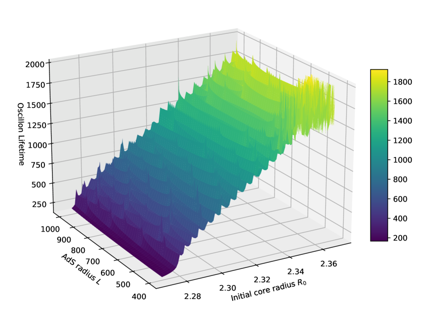
Figure 1: A plot of lifetimes of an AdS oscillon for $R_{0}$ and $L$.

As in [12], the resonances in the AdS oscillon lifetimes also exhibit the self-similar structure. Figure 2 shows the zoom-up of the region with $2.278\leq R_{0}\leq 2.280$ and $400\leq L\leq 500$ of Fig. 1. One can see a lot of small peaks and exhibit a self-similar structure. This self-similarity along the $R_{0}$-direction was found in [12]. A remarkable point here is that a self-similar structure can also be seen along the $L$-axis as well.

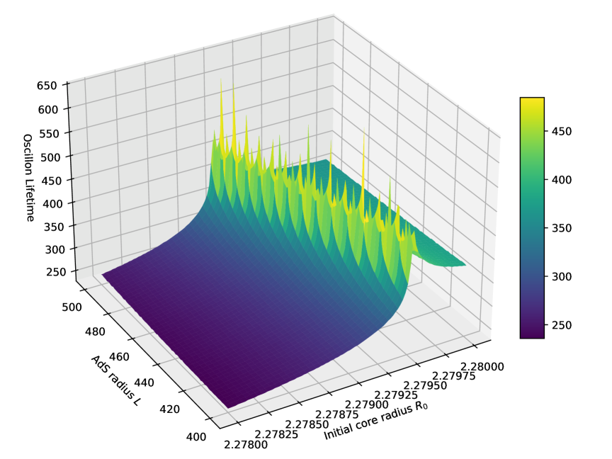
Figure 2: A zoom-up of the region with $2.278\leq R_{0}\leq 2.280$ and $400\leq L\leq 500$ in Fig. 1.

In the following, let us see the detailed properties of peaks by considering sections of Fig. 1 .

3.2 Peaks and exponents for $R_{0}$ with fixed $L$

Let us consider here a section with fixed $L$ . Figure 3 shows a section with $L=500$ and lifetimes of the AdS oscillon are plotted for values of the core size $R_{0}$ . There are three peaks in Fig. 3.

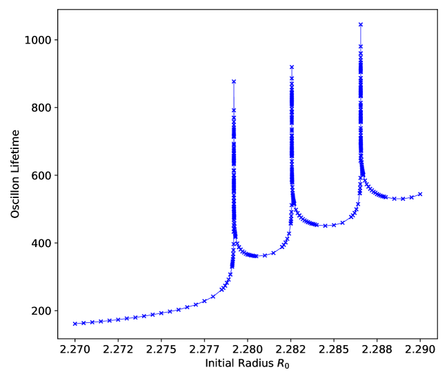
Figure 3: Lifetimes of the AdS oscillon for $R_{0}$ (fixed $L=500$).

Exponents

As in [12], for each of the peaks, one can define the exponents $\gamma_{\pm}$ for the left and right curves, respectively, as

$$\text{lifetime}~=~\left\{\begin{array}[]{ll}\gamma_{+}\,\ln(R_{0}-R_{0}^{\ast})+\mbox{const.}&\quad\mbox{(the right curve)}\\ \gamma_{-}\,\ln(R_{0}^{\ast}-R_{0})+\mbox{const.}&\quad\mbox{(the left curve)}\end{array}\right.\,,$$ (3.3)

where $R_{0}^{\ast}$ is the location of the peak on the $R_{0}$ line. The exponents can be numerically computed. Figure 4 shows the result for the peak with $R_{0}^{\ast}\approx 2.279$ . For the other peaks, the exponents can be computed similarly. The resulting exponents for the three peaks are summarized as

$$\begin{array}[]{c|ccc}~~R_{0}^{\ast}&2.279&2.282&2.286\\ \hline\cr\gamma_{+}&~~32.747&~~29.430&~~28.039\\ \gamma_{-}&32.660&31.297&32.746\end{array}\,.$$ (3.4)

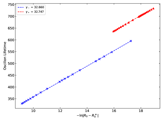
Figure 4: The exponents $\gamma_{\pm}$ of the peak with $R_{0}^{\ast}\approx 2.279$. The red (blue) marks are related to $\gamma_{+}~(\gamma_{-})$ .

3.3 Peaks and exponents for $L$ with fixed $R_{0}$

In this section, we consider a section with fixed $R_{0}$ . Figure 5 shows a section at $R_{0}=2.282$ and plots the lifetime of the AdS oscillon for values of AdS radius $L$. As plotted in Fig.5, we find resonance peaks along the $L$-direction for the AdS oscillon lifetimes.

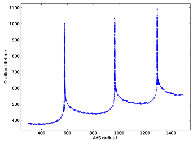
Figure 5: Lifetimes of the AdS oscillon for $L$ (fixed $R_{0}=2.282$).

Exponents

For the peaks in the $L$-direction, we introduce new exponents $\chi_{\pm}$ for the two branches of the curve, assigning $\chi_{-}$ to the left curve and $\chi_{+}$ to the right curve, as follows:

$$\text{lifetime}~=~\left\{\begin{array}[]{ll}\chi_{+}\,\ln(L-L^{\ast})+\mbox{const.}&\quad\mbox{(the right curve)}\\ \chi_{-}\,\ln(L^{\ast}-L)+\mbox{const.}&\quad\mbox{(the left curve)}\end{array}\right.\,.$$ (3.7)

Here, $L^{\ast}$ denotes the location of a peak. In Fig. 6, the exponents are computed from the lifetimes around the peak at $L^{\ast}\approx 578.160$. Performing the same calculations for the other peaks, we obtain

$$\begin{array}[]{c|ccc}~~L^{\ast}&578.160&966.567&1293.032\\ \hline\cr\chi_{+}&~~32.803&~~32.228&~~31.065\\ \chi_{-}&31.217&30.395&30.089\end{array}\,.$$ (3.8)

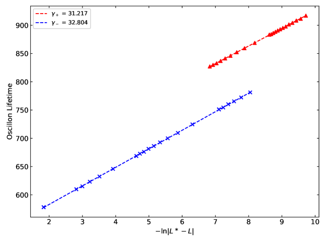
Figure 6: The exponents $\chi_{\pm}$ of the peak with $L^{\ast}\approx 578.160$. The red (blue) mark are concerned with values of $\chi_{+}~(\chi_{-})$ .

3.4 The bifurcation of peaks by reflected waves

Finally, we shall see the effect of the reflected waves against the resonance structures. Figure 7 shows lifetimes of the AdS oscillon for values of $L$ with fixed $R_{0}=2.36$ . For this value of $R_{0}$ , the effect of the reflected waves becomes significant. As a result, the resonance peaks exhibit the bifurcation. It seems likely that the bifurcation would present a certain pattern. It may be concerned with chaotic scattering [14], where the fractal structure appears in lifetimes.

Figure 7: Lifetimes of the AdS oscillon for $L$ (fixed $R_{0}=2.36$).

4 Conclusion and Discussion

In this letter, we have continued to study oscillons in AdS space and found new resonance structures for the curvature radius $L$ and the oscillon core size $R_{0}$ in lifetimes of the AdS oscillon. We then have computed the exponents associated with the resonance peaks by taking sections with fixed $L$ or $R_{0}$ . Finally, we have observed the bifurcation of the resonance peaks due to the reflected waves. It seems likely that the bifurcation has some pattern. It would be interesting to study it more carefully.

There are some future directions. It is desirable to understand the exponents of the peak curves analytically. For this issue, it may be interesting to consider the simplest oscillon constructed by Manton and Roma [17]. This oscillon was constructed in a real scalar field theory with a cubic potential in two-dimensional Minkowski spacetime and can be seen as a perturbative expansion around a sphaleron [18]. Hence one may get some analytical understanding of the exponents. The oscillon in [17] is constructed in two-dimensional Minkowski spacetime only, at least so far. So it is also interesting to construct the simplest oscillon in two-dimensional AdS space.

As an application, it is intriguing to consider a holographic interpretation of the resonances discussed here via the AdS/CFT correspondence [19]. In particular, in the AdS/QCD scenario [20, 21] the dilaton may exhibit fluctuations with longevity like oscillons before falling down to the stable configuration. The resonance structures may be related to some hadronic structures.

It is also interesting to include the gravitational back reaction by following [22]. The resonance structures may be bifurcated or destroyed by it.

We hope that the resonance structures found here would shed light on new aspects of the AdS/CFT correspondence.

Acknowledgments

The authors thank Takaaki Ishii, Tomohiro Shigemura and Norihiro Tanahashi for useful discussions and comments. The works of K. Y. were supported by MEXT KAKENHI Grant-in-Aid for Transformative Research Areas A “Machine Learning Physics” No. 22H05115, and JSPS Grant-in-Aid for Scientific Research (B) No. 22H01217 and (C) No. 25K07313.

References

- [1] I. L. Bogolyubsky and V. G. Makhankov, “On the Pulsed Soliton Lifetime in Two Classical Relativistic Theory Models,” JETP Lett. 24 (1976), 12 JINR-E2-9695.
- [2] V. G. Makhankov, “Dynamics of Classical Solitons In Nonintegrable Systems,” Phys. Rept. 35 (1978), 1-128.
- [3] M. Gleiser, “Pseudostable bubbles,” Phys. Rev. D 49 (1994), 2978-2981 [arXiv:hep-ph/9308279 [hep-ph]].
- [4] S. R. Coleman, “Q-balls,” Nucl. Phys. B 262 (1985) no.2, 263.
- [5] E. J. Copeland, M. Gleiser and H. R. Muller, “Oscillons: Resonant configurations during bubble collapse,” Phys. Rev. D 52 (1995), 1920-1933 [arXiv:hep-ph/9503217 [hep-ph]].
- [6] M. Gleiser and D. Sicilia, “Analytical Characterization of Oscillon Energy and Lifetime,” Phys. Rev. Lett. 101 (2008), 011602 [arXiv:0804.0791 [hep-th]].
- [7] M. Gleiser and D. Sicilia, “A General Theory of Oscillon Dynamics,” Phys. Rev. D 80 (2009), 125037 [arXiv:0910.5922 [hep-th]].
- [8] S. Y. Zhou, “Non-topological solitons and quasi-solitons,” Rept. Prog. Phys. 88 (2025) no.4, 046901 [arXiv:2411.16604 [hep-th]].
- [9] T. Ishii, T. Matsumoto, K. Nakano, R. Suda and K. Yoshida, “Oscillons in AdS space,” [arXiv:2412.19468 [hep-th]].
- [10] G. Fodor, P. Forgács and P. Grandclément, “Scalar field breathers on anti-de Sitter background,” Phys. Rev. D 89 (2014) no.6, 065027 [arXiv:1312.7562 [hep-th]].
- [11] P. Dorey, T. Romanczukiewicz, Y. Shnir and A. Wereszczynski, “Oscillons in gapless theories,” Phys. Rev. D 109 (2024) no.8, 085017 [arXiv:2312.05308 [hep-th]].
- [12] E. P. Honda and M. W. Choptuik, “Fine structure of oscillons in the spherically symmetric phi**4 Klein-Gordon model,” Phys. Rev. D 65 (2002), 084037 doi:10.1103/PhysRevD.65.084037 [arXiv:hep-ph/0110065 [hep-ph]].
- [13] M. Gleiser and M. Krackow, “Resonant configurations in scalar field theories: Can some oscillons live forever?,” Phys. Rev. D 100 (2019) no.11, 116005 doi:10.1103/PhysRevD.100.116005 [arXiv:1906.04070 [hep-th]].
- [14] J. M. Seoane, and M. AF. Sanjuan. “New developments in classical chaotic scattering,” Reports on Progress in Physics 76(1) (2012):16001-53.
- [15] O. Fukushima and K. Yoshida, “Chaotic instability in the BFSS matrix model,” JHEP 09 (2022), 039 [arXiv:2204.06391 [hep-th]].
- [16] O. Fukushima, T. Shigemura and K. Yoshida, “Scaling law for membrane lifetime,” Nucl. Phys. B 1017 (2025), 116946 [arXiv:2411.04754 [hep-th]].
- [17] N. S. Manton and T. Romańczukiewicz, “Simplest oscillon and its sphaleron,” Phys. Rev. D 107 (2023) no.8, 085012 [arXiv:2301.09660 [hep-th]].
- [18] F. R. Klinkhamer and N. S. Manton, “A Saddle Point Solution in the Weinberg-Salam Theory,” Phys. Rev. D 30 (1984), 2212.
- [19] J. M. Maldacena, “The Large N limit of superconformal field theories and supergravity,” Adv. Theor. Math. Phys. 2 (1998), 231-252 [arXiv:hep-th/9711200 [hep-th]].
- [20] U. Gursoy and E. Kiritsis, “Exploring improved holographic theories for QCD: Part I,” JHEP 02 (2008), 032 [arXiv:0707.1324 [hep-th]].
- [21] U. Gursoy, E. Kiritsis and F. Nitti, “Exploring improved holographic theories for QCD: Part II,” JHEP 02 (2008), 019 [arXiv:0707.1349 [hep-th]].
- [22] P. Bizon and A. Rostworowski, “On weakly turbulent instability of anti-de Sitter space,” Phys. Rev. Lett. 107 (2011), 031102 [arXiv:1104.3702 [gr-qc]].