Kira 3: integral reduction with efficient seeding and optimized equation selection

Abstract

We present version 3 of Kira, a Feynman integral reduction program for high-precision calculations in quantum field theory and gravitational-wave physics. Building on previous versions, Kira 3 introduces optimized seeding and equation selection algorithms, significantly improving performance for multi-loop and multi-scale problems. New features include convenient numerical sampling, symbolic integration-by-parts reductions, and support for user-defined additional relations. We demonstrate its capabilities through benchmarks on two- and three-loop topologies, showcasing up to two orders of magnitude improvement over Kira 2.3. Kira 3 is publicly available and poised to support ambitious projects in particle physics and beyond.

Keywords: Feynman diagrams, multi-loop Feynman integrals, integral reduction, computer algebra

11em() ZU-TH 39/25
HU-EP-25/17-RTG

NEW VERSION PROGRAM SUMMARY

Program title: Kira

Developer’s repository link: https://gitlab.com/kira-pyred/kira

Licensing provisions: GNU General Public License 3 (GPL)

Programming language: C++

Journal Reference of previous version:
P. Maierhöfer, J. Usovitsch and P. Uwer, Kira—A Feynman integral reduction program, Comput. Phys. Commun. 230 (2018) 99 [1705.05610].
J. Klappert, F. Lange, P. Maierhöfer and J. Usovitsch, Integral reduction with Kira 2.0 and finite field methods, Comput. Phys. Commun. 266 (2021) 108024 [2008.06494].

Does the new version supersede the previous version?: Yes.

Reasons for the new version: Improved algorithms with significant performance gains for all problems and new features.

Summary of revisions: The primary new feature is an improved seeding and selection of equations. Further improvements include the expanded support for numerical integration-by-parts applications, symbolic integration-by-parts reductions, and support for user-defined additional relations.

Nature of problem: The reduction of Feynman integrals to a smaller set of master integrals is a central building block for high-precision calculations of observables in theoretical particle and gravitational-wave physics. Furthermore, the reduction is a key ingredient in many methods to calculate the master integrals themselves.

Solution method: Kira generates a system of equations using integration-by-parts [1,2], Lorentz-invariance [3], and symmetry relations. It eliminates linearly dependent equations and identifies master integrals by solving the system over a finite field [4] and then solves the system of equation with Laporta’s algorithm [5]. Two solution methods are available: since version 1.0, Kira algebraically solves the system using Fermat [6]; since version 2.0, it numerically solves the system multiple times over finite fields, reconstructing master integral coefficients with FireFly [7,8]. Both approaches extend to any homogeneous linear system. New in this version, an optimized algorithm for seeding and selecting integration-by-parts identities demonstrates that a small subset of prior equations suffices for a full reduction.

References:

[1] F. V. Tkachov, A theorem on analytical calculability of 4-loop renormalization group functions, Phys. Lett. B 100 (1981) 65.

[2] K. G. Chetyrkin and F. V. Tkachov, Integration by parts: The algorithm to calculate $\beta$-functions in 4 loops, Nucl. Phys. B192 (1981) 159.

[3] T. Gehrmann and E. Remiddi, Differential equations for two-loop four-point functions, Nucl. Phys. B580 (2000) 485 [hep-ph/9912329].

[4] P. Kant, Finding linear dependencies in integration-by-parts equations: A Monte Carlo approach, Comput. Phys. Commun. 185 (2014) 1473 [1309.7287].

[5] S. Laporta, High precision calculation of multiloop Feynman integrals by difference equations, Int. J. Mod. Phys. A 15 (2000) 5087 [hep-ph/0102033].

[6] R. H. Lewis, Computer Algebra System Fermat, https://home.bway.net/lewis.

[7] J. Klappert and F. Lange, Reconstructing rational functions with FireFly, Comput. Phys. Commun. 247 (2020) 106951 [1904.00009].

[8] J. Klappert, S. Y. Klein and F. Lange, Interpolation of dense and sparse rational functions and other improvements in FireFly, Comput. Phys. Commun. 264 (2021) 107968 2004.01463.

Contents

1. 1 Introduction
2. 2 Preliminaries
3. 3 New features
   1. 3.1 Improved seeding
      1. 3.1.1 Changed behavior for sectors with symmetries or preferred master integrals
      2. 3.1.2 Truncating the seeds
   2. 3.2 Improved selection algorithm
   3. 3.3 Extra relations
   4. 3.4 Numerical sampling
   5. 3.5 Symbolic integration-by-parts reductions
   6. 3.6 Check master integral basis
4. 4 Further changes
   1. 4.1 Internal reordering of propagators
   2. 4.2 Support for 128-bit weights
   3. 4.3 Command Line option ----set_value
5. 5 Benchmarks
   1. 5.1 Double-box topologies
   2. 5.2 Tennis-court topology
   3. 5.3 Double-pentagon and pentagon-hexagon topologies
6. 6 Conclusions

1 Introduction

Feynman integrals are central objects for high-precision predictions for both particle physics experiments based on perturbative quantum field theory as well as for scattering events of cosmological objects like black holes which provide input for gravitational-wave studies. Calculations first generate amplitudes or angles consisting of tensor Feynman integrals which are then reduced to scalar Feynman integrals with the help of tensor reduction techniques. State-of-the-art calculations typically result in at least tens of thousands if not millions of scalar integrals whose direct calculations is infeasible in most cases. Integration-by-parts (IBP) identities [1, 2] and the Laporta algorithm [3] allow us to reduce this number to a significantly smaller set of master integrals. This is implemented in tools like AIR [4], FIRE [5, 6, 7, 8, 9], Reduze [10, 11], Kira [12, 13], FiniteFlow [14] with LiteRed [15, 16], and Blade [17].

The ever increasing need of higher precision leads to an increasing complexity both in terms of loop orders and external legs and, thus, requires constant development of new and improved integration-by-parts (IBP) reduction strategies. The field of Feynman integral reductions is constantly evolving and new techniques are explored and applied to integral reduction problems, e.g. syzygy equations/algebraic geometry [18, 19, 20, 21, 22, 23, 24, 25, 26, 27, 28], intersection numbers [29, 30, 31, 32, 33, 34, 35, 36, 37, 38, 39, 40, 41], finite field and interpolation techniques [42, 43, 44, 45, 8, 46, 14, 47, 48, 49, 50, 51, 52, 53, 54, 55], special integral representations [56, 57, 58, 17], and other methods [59, 60, 61] as well as machine learning techniques [62, 63, 64].

In this article we describe the new version 3 of Kira which is widely used in the community and backend in several public tools, see e.g. Refs. [65, 49, 66, 67, 68, 28]. After a brief recapitulation of IBP reductions and an overview of the strategy of Kira in Section˜2, we discuss the new features in Section˜3. The main features are improved seeding and selection strategies which reduce the reduction complexity significantly, especially if high tensor ranks are involved. Furthermore, we discuss other new features like the possibility to add additional relations, sample the system over user-provided finite field points, perform symbolic reductions, and check the master integral basis. In Section˜4 we discuss smaller changes with respect to the default behavior before quantifying the improvements with some benchmarks in Section˜5 and concluding in Section˜6.

2 Preliminaries

The central object of this paper is the Feynman integral

$$I_{\nu_{1},\ldots,\nu_{n}}\left(\{s_{i},m_{i}\},d\right)=\int\left(\prod_{j=1}^{L}\mathrm{d}^{d}k_{j}\right)\,\prod_{j=1}^{N}\frac{1}{D_{j}^{\nu_{j}}},$$ (1)

where we follow the standard notations used in Ref. [12]. We use the convention $D_{j}=q_{j}^{2}-m_{j}^{2}+\mathrm{i}\delta$, where $q_{j}$ denotes the momentum of the $j$-th propagator. The momentum $q_{j}$ can be written as a linear combination of $L$ loop momenta $k_{i}$ and $E$ linearly independent external momenta $p_{j}$ such that

$$q_{j}=\sum_{n=1}^{L}a_{jn}k_{n}+\sum_{n=1}^{E}b_{jn}p_{n}$$ (2)

for some integers $a_{jn}$ and $b_{jn}$. The term $\mathrm{i}\delta$ is the Feynman prescription. Here, $\{s_{i},m_{i}\}$ schematically denotes the set of external scales and internal masses on which the integral family depends. We work in dimensional regularization $d=d_{\mathrm{int}}-2\varepsilon$, where $d_{\mathrm{int}}$ is a positive (even) integer. In the remainder of this paper, we will typically leave the dependence on the external scales, masses, and the dimension implicit. The propagator exponents $\nu_{i}$ are assumed to be integers. The set of inverse propagators must be complete and independent in the sense that every scalar product of momenta can be uniquely expressed as a linear combination of $q_{j}$, squared masses $m_{j}^{2}$, and external kinematical invariants. The number of propagators is thus $N=\frac{L}{2}(L+2E+1)$ including auxiliary propagators that only appear with $\nu_{j}\leq 0$.

The Feynman integrals of Eq.˜1 are in general not independent. In Refs. [1, 2] it was found that they are related by so-called integration-by-parts (IBP) identities

$$\int\left(\prod\limits_{i=1}^{L}\mathrm{d}^{d}k_{i}\right)\frac{\partial}{\partial k^{\mu}_{i}}\frac{P^{\mu}_{j}}{D_{1}^{\nu_{1}}D_{2}^{\nu_{2}}\cdots D_{N}^{\nu_{N}}}=0,$$ (3)

where $P^{\mu}_{j}$ is either a loop momentum, an external momentum, or a linear combination thereof. In addition to these IBP identities, there also exist so-called Lorentz-invariance identities [69]

$$\sum_{i=1}^{E}\left(p_{i}^{\nu}\frac{\partial}{\partial p_{i\mu}}-p_{i}^{\mu}\frac{\partial}{\partial p_{i\nu}}\right)I_{\nu_{1},\ldots,\nu_{n}}=0.$$ (4)

They do not provide additional information, but it was found that they often facilitate the reduction process. Finally, there are symmetry relations between Feynman integrals which are most often searched for by comparing graph polynomials with Pak’s algorithm [70]. All these relations provide linear equations of the form

$$0=\sum_{i}c_{i}\left(\{s_{i},m_{i}\},d\right)I_{\nu_{1},\ldots,\nu_{n}}$$ (5)

between different Feynman integrals, where the coefficients $c_{i}\left(\{s_{i},m_{i}\},d\right)$ are polynomials in the kinematic invariants $s_{j}$, the propagator masses $m_{k}$, and $d$. The relations can be solved to express the Feynman integrals in terms of a basis of master integrals. It was even shown that the number of master integrals for the standard Feynman integrals of Eq.˜1 is finite [71].

Nowadays, the most prominent solution strategy is the Laporta algorithm [3]: The linear relations of Eq.˜5 are generated for different values of the propagator powers $\nu_{j}$ resulting in a system of equations between specific Feynman integrals. Each choice of $\{\nu_{j}\}$ is called a seed and this generation process is also known as seeding. The system can then be solved with Gauss-type elimination algorithms.

This requires an ordering of the integrals. In Kira we first assign the integrals to so-called topologies based on their respective sets of propagators, i.e. their momenta and masses. We assign a unique integer number to each topology. Secondly, we assign each integral to a sector

$$S=\sum\limits_{j=1}^{N}2^{j-1}\,\theta(\nu_{j}-\tfrac{1}{2}),$$ (6)

where $\theta(x)$ is the Heaviside step function. A sector $S$ (with propagators powers $\nu_{j}$) is called subsector of another sector $S^{\prime}$ (with propagators powers $\nu^{\prime}_{j}$) if $S<S^{\prime}$ and $\theta(\nu_{j}-\tfrac{1}{2})\leq\theta(\nu^{\prime}_{j}-\tfrac{1}{2})$ for all $j=1,\dots,N$. We denote as top-level sectors those sectors which are not subsectors of other sectors that contain Feynman integrals occurring in the reduction problem at hand. For the discussions in the following sections it is beneficial to use the big-endian binary notation instead of the sector number defined by Eq.˜6, i.e. the sector $S=5$ is represented by b$1010$ where each number represents one bit of the number $5$ in reverse order. In this notation it is immediately visible that b$1010$ is a subsector of b$1110$.

Furthermore, it is useful to define the number of propagators with positive powers,

$$t=\sum_{j=1}^{N}\theta(\nu_{j}-\tfrac{1}{2}),$$ (7)

and

$$r=\sum_{j=1}^{N}\nu_{j}\theta(\nu_{j}-\tfrac{1}{2}),\qquad s=-\sum_{j=1}^{N}\nu_{j}\theta(\tfrac{1}{2}-\nu_{j}),\qquad d=\sum_{j=1}^{N}(\nu_{j}-1)\theta(\nu_{j}-\tfrac{1}{2})$$ (8)

denoting the sum of all positive powers, the negative sum of all negative powers, and the sum of positive powers larger than 1 (referred to as dots), respectively.

On the one hand, these concepts allow us to order the integrals in Kira. On the other hand, they are used to limit the seeds $\{\nu_{j}\}$ for which equations are generated. We generate the equations only for those sets $\{\nu_{j}\}$ for which $r\leq r_{\mathrm{max}}$, $s\leq s_{\mathrm{max}}$, and $d\leq d_{\mathrm{max}}$, where $r_{\mathrm{max}}$, $s_{\mathrm{max}}$, and $d_{\mathrm{max}}$ are input provided by the user.

The workflow in Kira is split into two components: first generating the system of equations and then solving it. We offer two different strategies for the latter. First, the system can be solved analytically using the computer algebra system Fermat [72] for the rational function arithmetic. Secondly, the system can be solved using modular arithmetic over finite fields [42, 43, 44, 45] with our internal solver pyRed. The variables, i.e. kinematic invariants and masses, are replaced by random integer numbers and all arithmetic operations are performed over prime fields. Choosing the largest $63$-bit primes allows us to perform all operations on native data types and to avoid large intermediate expressions. The final result can then be interpolated and reconstructed by probing the system sufficiently many times for different random choices of the variables. We employ the library FireFly for this task [46, 47].

The main improvements of Kira 3 concern the generation of the system of equations and it is thus beneficial for the understanding of the reader to summarize the old algorithm from version 2.3 in more detail:

1. Identify trivial sectors and discard all integrals in these sectors.

2. Identify symmetries between sectors including those of other integral families and collect them in the set $\{S^{\prime}\}$.

3. Generate IBP equations for all sectors not in $\{S^{\prime}\}$ and generate only symmetry equations for all sectors in $\{S^{\prime}\}$. Start from the simplest one and generate all equations within the specifications provided by the user:

   1. Generate one equation. Check if it is linearly independent by inserting all previously generated equations numerically [43].

   2. Keep, if it is linearly independent, otherwise drop it.

4. After all equations were generated, solve the system for the target integrals specified by the user with modular arithmetic and drop all equations which do not contribute to their solutions.

At the end of this procedure Kira has generated a system of linearly independent equations specifically trimmed to suffice to reduce the target integrals to master integrals.

3 New features

3.1 Improved seeding

The choice of which equations should be generated for the reduction has severe impact on the performance of the reduction. Previous versions of Kira seed conservatively and generate all equations within the bounds specified by the user to reduce to the minimal basis of master integrals. Irrelevant equations are filtered out through a selection procedure. However, for integrals with many loops or high values of $r$, $s$, and $d$ the combinatorics of the seeds easily gets out of hand and already makes the generation of the system of equations unfeasible, running both into runtime and memory limits.

We show that it is possible to find a subset of relevant equations which improves the generation of equations lifting the limits for many applications, as demonstrated in Refs. [73, 74]. We revise the seeding process in Kira and identify three areas for improvement: sectors related by symmetries, sectors containing preferred master integrals, and subsectors. We discuss the first two points in Section˜3.1.1 and the latter in Section˜3.1.2.

3.1.1 Changed behavior for sectors with symmetries or preferred master integrals

In previous versions of Kira, sectors which are related by symmetries to other sectors are seeded with the same values for $r_{\mathrm{max}}$ and $s_{\mathrm{max}}$, ignoring any set $d_{\mathrm{max}}$. Similarly, sectors which contain one of the preferred master integrals are seeded with the maximum values of $r_{\mathrm{max}}$ and $s_{\mathrm{max}}$ for all sectors, again ignoring $d_{\mathrm{max}}$. Those choices turn out to be too conservative and negatively impact the performance of IBP reductions. With Kira 3 subsectors inherit the values for $r_{\mathrm{max}}$, $s_{\mathrm{max}}$, and also $d_{\mathrm{max}}$ from higher sectors, independently of symmetries and preferred master integrals.

Furthermore, in previous versions Kira did not generate IBP equations for sectors which can be mapped away by symmetries and instead relied on symmetry relations alone. While this is a good strategy to generate fewer equations, symmetry equations quickly become longer with more complicated coefficients when they are generated with numerators. Their complexity easily overtakes those of IBP equations even for moderate values of $s$ and makes the solution significantly more expensive. Hence, with Kira 3 we also generate IBP equations for sectors which are mapped away by symmetries. This increases the reduction performance, while the growth of generated equations is easily compensated by the new truncation option discussed in the next subsubsection.

3.1.2 Truncating the seeds

By default, the values for $r_{\mathrm{max}}$ and $s_{\mathrm{max}}$ for one sector are inherited by all subsectors. For example, if we are interested in the integral $T(1,1,1,1,1,1,1,0,-4)$, the typical choice is to seed the sector b$111111100$ with $r_{\mathrm{max}}=7$ and $s_{\mathrm{max}}=4$. This then propagates to the lower sectors and sector b$111111000$ is automatically seeded with $r_{\mathrm{max}}=7$, corresponding to $d_{\mathrm{max}}=1$, and $s_{\mathrm{max}}=4$ and sector b$111000000$ with $r_{\mathrm{max}}=7$, corresponding to $d_{\mathrm{max}}=4$, and $s_{\mathrm{max}}=4$, respectively. The increase in $d_{\mathrm{max}}$ can already be restricted by manually setting $d_{\mathrm{max}}$ (with the exceptions discussed in Section˜3.1.1), but we previously argued against this to prevent finding too many master integrals. With the new release of Kira 3 we revise this recommendation and encourage setting $d_{\mathrm{max}}$.

However, keeping $s_{\mathrm{max}}$ constant when descending to the subsectors is even more problematic because the combinatorics of distributing irreducible scalar products in lower sectors grows factorially. As it turns out, most of these seeds are actually not required to reduce integrals with positive $s$ in higher sectors and one can decrease $s_{\mathrm{max}}$ in lower sectors. In Kira 3 we introduce a new feature to restrict $s$ following the function

$$s\leq\max(1,\ t-l+1,\ s_{\text{max},\text{sector}})$$ (9)

where $t$ was defined in Eq.˜7, $l$ can be chosen by the user, and $s_{\text{max},\text{sector}}$ is the value that was explicitly set by the user for this sector with the option reduce. If no explicit value is provided with reduce, $s_{\text{max},\text{sector}}=0$, i.e. it is not inherited from higher sectors. The usefulness of this feature was first described and proven in Ref. [73]. Similar observations were also made by the developers of Blade [17] and FIRE [75].

This feature can be enabled with the new job file option

    truncate_sp:
      - {topologies: [<topologies>], l: <n>}

with the two arguments

• topologies (optional): a list of topologies to which truncate_sp should be applied. If no topology is provided, Kira applies truncate_sp to all topologies.

• l (mandatory): This option takes the integer argument <n> (negative numbers are allowed) and instructs Kira to choose seeds following Eq.˜9 with $l=\texttt{<n>}$.

A good choice of <n> can result in a speedup of orders of magnitude. To choose the optimal parameters we recommend the following strategy:

1. The highest possible value for <n> is computed by taking the difference between the $t$ value of the top-level sector and the highest number $s$ of an integral which one wants to reduce. This choice is too optimistic in almost all cases and one should run Kira to check if all integrals reduce to the expected master integrals. The new option check_masters described in Section˜3.6 is helpful for this purpose. If too many master integrals are reported, we recommend to tune the options provided to Kira starting with those sectors with the highest value of $t$ that report too many master integrals.

2. Tune all sectors at level $t$:

   1. If many or even all sectors with the same value of $t$ have too many master integrals whose values are cut off by Eq.˜9, decrease <n> to a value that seeds those additional master integrals.

   2. If only a few sectors have too many master integrals cut off by Eq.˜9 or $s>s_{\mathrm{max}}$, increase $s_{\mathrm{max}}$ for the sector.

   3. If there are too many master integrals with $d>d_{\mathrm{max}}$ in a sector, increase $d_{\mathrm{max}}$ for this sector.

3. Run Kira again to check if there are additional master integrals on level $t$. If yes, tune those sectors further by repeating steps 2 and 3. If not, reduce $t$ by one and repeat steps 2 and 3 on this level.

Using the option select_mandatory_recursively is not recommended if truncate_sp is enabled because the aforementioned option selects all integrals to reduce with a constant value of $s_{\mathrm{max}}$. This results in Kira reporting many unreduced integrals because many required seeds are removed by truncate_sp.

Summarizing this section, our recommendation for the job file with Kira 3 reads

jobs:
 - reduce_sectors:
    reduce:
      - {topologies: [topo7], sectors: [b111111100], r: 7, s: 5, d: 0}
      - {topologies: [topo7], sectors: [b011100100], r: 5, s: 3, d: 1}
    truncate_sp:
      - {topologies: [topo7], l: 3}
    select_integrals:
      select_mandatory_list:
        - [seeds7]

for the example topology topo7 provided with the source code. The top-level sector b111111100 (127) is seeded with $r_{\mathrm{max}}=7$, $s_{\mathrm{max}}=5$, and $d_{\mathrm{max}}=0$, providing sufficient seeds to reduce all integrals in this sector. Furthermore, truncate_sp cuts away seeds in subsectors. However, sector b011100100 (78) had to be tuned by increasing $d_{\mathrm{max}}$ to $1$.

3.2 Improved selection algorithm

Once Kira determines the linearly independent system of equations, it will select the relevant equations to reduce specific integrals as defined for example with the option select_integals. The algorithm to select relevant equations in previous Kira versions is not optimal. One weakness can easily be illustrated when reducing all integrals in the top-level sector b111111100 (127) of the topology topo7 depicted in Fig.˜1 with exactly $s=5$.

Figure 1: The planar double box topo7 contributing, e.g., to single-top production.

With Kira 2.3, we first seed with $s_{\mathrm{max}}=5$ and, secondly, with $s_{\mathrm{max}}=6$, and in both cases select equations to reduce the same set of integrals. As can be seen in Table˜1, the number of selected equations and with it the number of terms as well as the time to solve the system increases.

Table 1: Comparison of the generated and selected systems for topo7 when seeded with different values of $s_{\mathrm{max}}$.

	2.3, $s_{\mathrm{max}}=5$	2.3, $s_{\mathrm{max}}=6$	3.0, $s_{\mathrm{max}}=5$	3.0, $s_{\mathrm{max}}=6$
# of generated eqs.	3 317 357	6 009 193	4 053 617	7 511 785
# of selected eqs.	62 514	85 119	30 984	30 984
# of terms	461 336	659 803	245 975	245 975

This can be explained by the fact that Kira generates and selects equations with the sector-by-sector approach as discussed in Section˜2. It prefers equations generated with higher values for $r$, $s$, and $d$ in lower sectors, which are usually more complicated than equations generated with low values of $r$, $s$, and $d$ in higher sectors.

Secondly, we identified another problem: Kira selects equations which do not contribute to the final result because they cancel in intermediate steps. This can be illustrated with the toy system

$$(\mathrm{i})\quad 0= \,x[6]+b_{1}\,x[2],$$ (10)

$$(\mathrm{ii})\quad 0= \,x[6]+c_{1}\,x[1],$$

$$(\mathrm{iii})\quad 0= \,x[5]+a_{1}\,x[2]+a_{2}\,x[4]+a_{3}x[3],$$

$$(\mathrm{iv})\quad 0= \,x[5]+a_{1}\,x[2],$$

where $x[i]$ represents a Feynman integral and the Roman number in front denotes the equation number. We now solve this system using Gaussian elimination.

In Kira we solve equations one at a time, starting with equation $(\mathrm{iv})$ in Eq.˜10 and work in a bottom-up approach. Whenever we add a new equation, Kira immediately inserts already known solutions into the new equation. If the equation equates to zero, it is treated as redundant and is discarded. Otherwise its terms are sorted with respect to some Laporta ordering and the new equation is added to the solved equations. This is repeated until all equations are processed. This step is called forward elimination in Kira and results in a system that is in upper-triangular form. After the forward elimination Eq.˜10 reads

$$(\mathrm{i})\quad 0= \,b_{1}\,x[2]-c_{1}\,x[1]\quad \{\mathrm{ii}\}$$ , (11)

$$(\mathrm{ii})\quad 0= \,x[6]+c_{1}\,x[1]\quad \{\}$$ ,

$$(\mathrm{iii})\quad 0= \,a_{2}\,x[4]+a_{3}\,x[3]\quad \{\mathrm{iv}\}$$ ,

$$(\mathrm{iv})\quad 0= \,x[5]+a_{1}\,x[2]\quad \{\}$$ .

Kira traces which equations were used to eliminate integrals from the newly added equation, in this example denoted by the Roman numbers in the curly brackets: Equation $(\mathrm{ii})$ was used to eliminate the integral $x[6]$ in equation $(\mathrm{i})$ and equation $(\mathrm{iv})$ was used to eliminate the integral $x[5]$ in equation $(\mathrm{iii})$.

In the second step, the backward substitution iterates the system of equations bottom-up and inserts all available solutions. Again we record each equation used to eliminate integrals. After the back substitution we obtain

$$(\mathrm{i})\quad 0= \,b_{1}\,x[2]-c_{1}\,x[1]\quad \{\mathrm{ii}\}$$ , (12)

$$(\mathrm{ii})\quad 0= \,x[6]+c_{1}\,x[1]\,\quad \{\}$$ ,

$$(\mathrm{iii})\quad 0= \,a_{2}\,x[4]+a_{3}\,x[3]\quad \{\mathrm{iv}\}$$ ,

$$(\mathrm{iv})\quad 0= \,x[5]+a_{1}\,c_{1}/b_{1}\,x[1]\quad \{\mathrm{i},\mathrm{ii}\}$$ .

Here equation $(\mathrm{i})$ is used to eliminate the integral $x[2]$ in equation $(\mathrm{iv})$.

In previous versions the information in the curly brackets from Eq.˜12 is used to select relevant equations for the reduction process. For the reduction of the integral $x[4]$, the previous versions of Kira selected equation $(\mathrm{iii})$ because it provides the solution for $x[4]$, then equation $(\mathrm{iv})$ which was inserted into equation $(\mathrm{iii})$, and finally equations $(\mathrm{i})$ and $(\mathrm{ii})$ which were inserted into equation $(\mathrm{iv})$. However, the latter two do not provide any relevant information: it is easy to spot in Eq.˜10 that equation $(\mathrm{iii})$ contains equation $(\mathrm{iv})$ as a subequation. This subequation thus vanishes after inserting equation $(\mathrm{iv})$ only and the information of equations $(\mathrm{i})$ and $(\mathrm{ii})$ is not needed. We call this phenomenon hidden zero which in general can take more complicated forms.

To address both the deficits of the sector-by-sector approach and the hidden zeros, Kira 3 selects the relevant equations after the forward elimination only. For the example above we can clearly see that this information in Eq.˜11 is sufficient to reduce the integral $x[4]$ to master integrals and it gives the relevant equations only. For more generic examples the algorithm requires one additional step: Kira reduces the system numerically over a finite field once and checks if the selected equations are sufficient to reduce all integrals to the minimal basis of master integrals. All unreduced integrals are added to the list and the reduction is repeated until all requested integrals are reduced to the minimal basis. This algorithm is generic and applies to user-defined systems as well.

However, it cannot give the minimal number of equations for general problems as more stealthy zeros in the forward elimination remain undetected. One could heuristically reduce the number of equations by randomly reordering the equations and repeating the algorithm discussed above, throwing out all irrelevant equations at the end of every iteration. Repeating this process, we end up with less and less equations until reaching a local minimum. However, a randomly reordered system of equations typically gets dense after a few Gaussian elimination steps, making the solution computationally expensive. One could reorder the system of equations in bunches, e.g. in batches of 20 equations, but in our experiments this yield at most $20$ % less equations. This is a very low improvement from our perspective and does not justify the implementation of this algorithm yet. There is another algorithm, privately called the Oerlikon algorithm, designed to select necessary IBP equations, see Refs. [24, 27], which we plan to investigate with Kira in the future.

The impact of the new selection algorithm is illustrated in Table˜1. Since the new truncation discussed in Section˜3.1.2 option is not enabled, Kira 3 generates more equations than Kira 2.3 as discussed in Section˜3.1.1. However, even though $22$ % more equations are generated for $s_{\mathrm{max}}=5$, the new selection algorithm actually selects $50$ % less equations, indicating that many hidden zeros and irrelevant equations are dropped. Moreover, increasing $s_{\mathrm{max}}$ to $6$ does not change the selected equations anymore as in previous versions.

3.3 Extra relations

There can be additional relations between integrals that are not discovered by Kira, usually through some non-trivial symmetries, see e.g. Refs. [76, 77, 78], or four-dimensional kinematic constraints, see e.g. Ref. [79]. Therefore, it is desirable to add those relations to the system generated by Kira. In previous version additional relations could only be added in the user-defined system mode. With Kira 3 it is now possible to add them during the normal reduction setup with the option extra_relations: <file> in the job file. It takes exactly only one file as argument in which the relations should be provided in the format of user-defined systems as described in Ref. [13]. The additional equations are inserted after the IBP relations for a specific sector were generated. Additional relations belonging to sectors beyond the seeded sectors are inserted at the end of the generation process.

3.4 Numerical sampling

For complicated reductions it might be useful to sample the reduction numerically on chosen phase space points, either before attempting to obtain full analytic expressions or bypassing them altogether, see e.g. Ref. [80]. In the context of Kira this feature has been explored in Ref. [79].

There are two aspects with respect to this feature: First, we implemented an interface for the user to provide both the prime for the finite field and the sample points with the option numerical_points: <file> where the file format reads

prime 9223372036854771977
d s t m12 m22
11111 -1 -38 -1039/6 -2712776
11112 -1 -38 -1039/6 -2712776

prime 9223372036854771689
d s t m12 m22
11111 -1 -38 -1039/6 -2712776
11112 -1 -38 -1039/6 -2712776

The first line specifies the user-defined prime number for a finite field. The largest prime number currently permitted is $9223372036854775783$, i.e. the largest $63$-bit prime. The second line lists all symbols that the user intends to assign numerical values to. It should contain all symbols appearing in the system, i.e. all kinematic invariants, the dimension $d$, and potentially further symbols in user-defined systems of equations. In the following lines the numerical values corresponding to those symbols are provided. An empty line separates the collection of points from another collection of points in a different prime field.

The second, less obvious aspect concerns the generation of the system of equations by Kira. By default Kira chooses pseudo-random numbers for all symbols in the system during the generation step to check the equations for linear dependence. However, the user might restrict the sample points to a slice in phase space in which not all of the symbols are independent. In this case, further cancellations can occur and a system of linearly-independent equations generated on a general pseudo-random phase space point might no longer contain sufficient information to reduce all integrals. Therefore, when instructed with numerical_points in the job file, Kira generates the system with the first provided phase space point and prime and writes it to disk as usual. The same result can be obtained with the command-line options ----set_value and ----prime_user, see also Section˜4.3. By default, Kira writes the system to disk with algebraic coefficients, but can be instructed to replace all symbols by the given values with the job file option symbols2num: true.

The results of the numerical reductions are written to the files results/<topology>/<input file name>_<prime>_<j>.m. Since we want to avoid to produce too large files, only 1000 entries are written into each file. If this limit is reached, Kira writes to the next file with j increased by one. An example output for a reduction with the example integral family topo7 looks like

{9223372036854771977,
  {{11111, 9223372036854771976, 9223372036854771939, 7686143364045643141,
  9223372036852059201},
    {
      {topo7[1,1,1,1,1,1,1,-5,0],
        {topo7[1,1,1,1,1,1,1,0,-1], 2951302433002828169},
        {topo7[1,1,1,1,1,1,1,-1,0], 819004719938417371},
        {topo7[1,1,1,1,1,1,1,0,0], 5495110817388584284},
        ...
      },
      ...
    }
  },
  {{11112, 9223372036854771976, 9223372036854771939, 7686143364045643141,
  9223372036852059201},
    {
      {...}
    }
  }
}

where the indentation is for better illustration. Each file is structured as a nested list in Mathematica readable format. The first entry is a prime number used in the computations, followed by sublists, each containing IBP results for a specific numerical point. Each sublist starts with the numerical point as an identifier (note that the user input has been converted into a finite field element over the user provided prime), followed by the numerical reduction results. Each reduction result is a sublist beginning with the integral to be reduced, followed by pairs of master integrals and their corresponding reduction coefficients.

3.5 Symbolic integration-by-parts reductions

Obtaining general recurrence relations for arbitrary propagator powers can be seen as the ultimate goal for IBP reductions since they should facilitate an efficient reduction for all integrals of a family. LiteRed [15, 16] is the only public tool that offers an algorithm to search for such relations, but it is not guaranteed to succeed. Recently, a different strategy has been explored in Ref. [60].

In Kira 3 it is now possible to treat propagator powers symbolically and use the Laporta strategy to derive symbolic recursion relations. Every power is treated as an additional symbol which makes it computationally expensive to derive fully algebraic recursion relations in all indices. However, constructing recursion relations for one or very few powers works reasonably well in many problems. This feature is activated with the option symbolic_ibp: [<n1>, <n2>, ...] in integralfamilies.yaml. <n1>, <n2>, …may take an integer number between $1$ and the total number of propagators provided with the integral family definition. The symbolic power is then associated with the n1, n2, …propagator from top to bottom as listed in integralfamilies.yaml.

In the following we illustrate our best strategy for a symbolic IBP reduction as applied in Ref. [81] with an example available in the directory examples/symbolic_IBP provided with the source code. It is advised to take as a top-level sector all propagators which have positive propagator powers, but to omit the propagators associated with the symbolic powers. The relevant part of integralfamilies.yaml may read

top_level_sectors: [b011111100] # b011111100 is same as sector 126
symbolic_ibp: [1]

where we treat the first propagator power as a symbolic power. The example job file jobs_lowering.yaml is used to generate lowering relations for the symbolic power:

jobs:
 - reduce_sectors:
    reduce:
      - {topologies: [topo7], sectors: [b011111100], r: 7, s: 2, d: 1}
    truncate_sp:
      - {topologies: [topo7], l: 4}
    select_integrals:
      select_mandatory_list:
        - [toReduce_lowering]
    preferred_masters: masters_lowering
    integral_ordering: 2
    run_initiate: true
    run_firefly: true
 - kira2math:
    target:
     - [toReduce_lowering]

The file toReduce_lowering contains one integral which will be reduced with Kira:

#to reduce
topo7[0,1,1,1,1,1,1,-2,0]

The essential master integrals are listed in the file masters_lowering:

topo7[-1,1,1,1,1,1,1,0,0]
topo7[-1,1,1,1,1,1,1,0,-1]
topo7[-1,1,1,1,1,1,1,-1,0]
topo7[-2,1,1,1,1,1,1,0,0]

Since the first index is symbolic, the corresponding entries are interpreted as lowering or raising operations. The first indices of the selected integrals serve as starting point and, if all of them are larger than the first indices of all preferred master integrals, Kira will construct lowering relations, and raising operations if the first indices of the selected integrals are smaller. In the example above Kira will try to construct a lowering relation shifting the first index down by $-1$ and $-2$. If all of the selected integrals and all of the preferred master integrals have zero or negative symbolic indices, the corresponding sector is merged with a subsector, generating less equations. In the example above sectors b011111100 (126) and b111111100 (127) are considered to be the same.

In the resulting expressions, the symbols b0, …,b(N-1) denote symbolic powers, where N is the total number of propagators listed in integralfamilies.yaml. In the example above, we encounter the relation

topo7[0,0,1,0,0,0,1,-1,0] ->
 + topo7[-1,0,1,0,0,0,1,0,0]*(((d+(-2))*(1))/((b0+(-1))*(1)))

in the results directory, which can be translated into the recursion relation

$$\texttt{topo7}(b_{0},0,1,0,0,0,1,-1,0)\rightarrow\frac{d-2}{b_{0}-1}\texttt{topo7}(b_{0}-1,0,1,0,0,0,1,0,0)$$ (13)

in the first $b_{0}$ index.

3.6 Check master integral basis

In many cases users determine and choose the basis of master integrals before performing a full-fledged reduction. Criteria might be a convenient basis choice for the reduction and/or for solving the master integrals. Since version 1.1, Kira allows users to provide their basis choice with the job file option preferred_masters. Since version 2.0, the basis can also consist of linear combinations of master integrals as described in Ref. [13]. However, by default Kira supplements the provided basis with additional master integrals in case it cannot reduce to the provided basis. With the new job file option check_masters: true, Kira 3 compares the master integrals it found when generating the system with those provided by preferred_masters. It reports both additional master integrals as well as those provided master integrals it does not need for the reduction. In case it finds additional master integrals, it aborts the reduction and throws an error.

This feature is especially useful if users already determined the basis and try to exploit the new seeding features discussed in Section˜3.1 to generate an optimal system of equations.

4 Further changes

4.1 Internal reordering of propagators

It is well known that the definition of the propagators in Eq.˜1 influences the performance of the reduction. Not only different choices for the momenta have an impact, simply reordering them can make a difference, especially when selecting equations before the actual reduction as in Kira. This can be demonstrated with the four-loop propagator topology depicted in Fig.˜2.

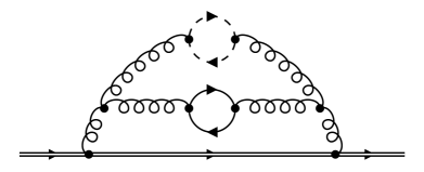
Figure 2: Four-loop propagator topology with two masses.

We reduce all integrals appearing in the quark self energy amplitude for the relation between the quark mass renormalization constants in the $\overline{\text{MS}}$ and the on-shell schemes [82]. We compare the propagator order

$$\begin{split}&p_{1}^{2}-m_{1}^{2},\ (p_{1}-q)^{2},\ \underline{(p_{2}+p_{3})^{2}},\ (p_{1}-p_{3}+p_{4}-q)^{2},\ (p_{3}-p_{4})^{2},\ \underline{(p_{3}+q)^{2}},\ \underline{(p_{2}+p_{4})^{2}},\\ &p_{2}^{2}-m_{2}^{2},\ (-p_{1}+p_{2}+p_{3}-p_{4}+q)^{2}-m_{2}^{2},\ p_{3}^{2},p_{4}^{2},\ \underline{(p_{1}+p_{3})^{2}},\ \underline{(p_{1}+p_{4})^{2}},\ \underline{(p_{1}+p_{2})^{2}},\end{split}$$ (14)

which was automatically chosen when generating the amplitude in Ref. [82], denoted as bad choice, with propagator order 1,

$$\begin{split}&p_{3}^{2},\ p_{4}^{2},\ p_{1}^{2}-m_{1}^{2},\ p_{2}^{2}-m_{2}^{2},\ (p_{1}-q)^{2},\ (p_{3}-p_{4})^{2},\ (p_{1}-p_{3}+p_{4}-q)^{2},\\ &(-p_{1}+p_{2}+p_{3}-p_{4}+q)^{2}-m_{2}^{2},\ \underline{(p_{2}+p_{3})^{2}},\ \underline{(p_{3}+q)^{2}},\ \underline{(p_{2}+p_{4})^{2}},\ \underline{(p_{1}+p_{3})^{2}},\\ &\underline{(p_{1}+p_{4})^{2}},\ \underline{(p_{1}+p_{2})^{2}},\end{split}$$ (15)

which implements the guidelines outlined in Ref. [83]: order by the number of momenta and put massless propagators first. The underlined entries denote auxiliary propagators which only appear in the numerator and should be placed at the end.

When comparing the systems of equations generated with Kira 3 for the two permutation ordering choices in Table˜2, we see that the system generated with order 1 selects 3 % less equations, 6.5 % less terms, and can be solved 29 % faster for a phase space point over a finite field than the system generated with the bad choice.

Table 2: Comparison of the generated and selected systems of equations for the two propagator orders defined in Eqs.˜14 and 15 of the four-loop propagator topology depicted in Fig.˜2.

	bad choice	order 1
# of equations	481 855	467 338
# of terms	5 902 637	5 537 560
$T_{\texttt{pyRed}{}}$	8.0 s	6.2 s

Since version Kira 2.3 offers the possibility to reorder the propagators internally independent of the order specified in the integral family definition, i.e. the propagator order in the input and output files differs from the order Kira uses internally to perform the reduction. The ordering can either be chosen manually or be adjusted automatically according to four different ordering schemes. The one outlined above usually provides the best results. With Kira 3 we will automatically turn on this ordering scheme by default. It can be overridden in config/integralfamilies.yaml by choosing a different ordering scheme with the option permutation_option: <N>, with <N> taking values from 1 to 4, or by manually fixing the order with the option permutation: [<n1>,…,<nN>], where each <ni> denotes the number of the i’th propagator defined for the topology.

4.2 Support for 128-bit weights

Internally Kira represents all integrals by an integer weight. Up to Kira 2.2 they were limited to native 64-bit integers. However, those do not suffice to represent all integrals for some new, ambitious projects, see e.g. Ref. [81]. Hence, with Kira 2.3 we introduced 128-bit weights based on compiler extensions available in standard C++ compilers like GCC [84] and clang [85]. The width of the weights can be set with

meson setup -Dweight_width=<WIDTH> build

when compiling Kira, where <WIDTH> can either be 64 (default) or 128. If 128 is chosen, the executable is called kira128.

Note that sectors are still represented by a 32-bit integer and, thus, topologies with more than 31 lines are not yet supported.

4.3 Command Line option ----set_value

When generating a system of equations with previous versions of Kira, a pseudo-random point was selected to determine the linearly independent system. The old implementation of ----set_value did not influence this point. In the same way as the job file option numerical_points introduced in Section˜3.4, Kira 3 now ensures that user-defined numerical points are respected during the generation and selection steps. In combination with the job option symbols2num: false the resulting independent system of equations is written to disk with symbolic coefficients.

5 Benchmarks

We provide multiple examples for two-loop and three-loop reductions in the example directory shipped with the source code, in which the option truncate_sp as introduced in Section˜3.1 and the new equation selection discussed in Section˜3.2 are demonstrated,

• double-box: topo7 and topo5, see Figs.˜3(a) and 3(b),

• tennis-court: TennisCourt, see Fig.˜3(c),

• double-pentagon: doublePentagon, doublePentagon-1-mass, doublePentagon-2-mass, doublePentagon-3-equal-mass, see Figs.˜3(d), 3(e), 3(f) and 3(g),

• pentagon-hexagon: hex, see Fig.˜3(h).

(a) topo7

(b) topo5

(c) TennisCourt

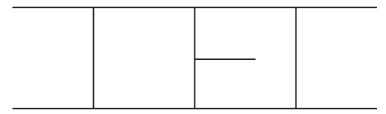
(d) massless doublePentagon

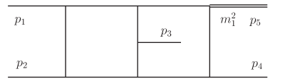
(e) one mass doublePentagon

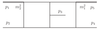
(f) two mass doublePentagon

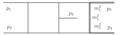
(g) three equal mass doublePentagon

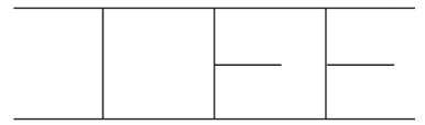
(h) hex

Figure 3: Illustrated are different families which are used to study the algorithms as implemented in Kira 3. Integral family 3(a) and 3(b), are double-box topologies and are called topo7 and topo5, respectively. Integral family 3(c) is a three-loop tennis-court topology, called TennisCourt. The integral family depicted in 3(d)-3(g) belong to a double-pentagon topology and are called doublePentagon. Integral family 3(h) is a two loop pentagon-hexagon family with the name hex. The external momenta $p_{i}$, are explicitly depicted to avoid ambiguity. Variables $m_{i}$ are used to denote massive lines.

To identify individual reduction problems we use the notation ${r_{\mathrm{max}}.s_{\mathrm{max}}.d_{\mathrm{max}}}$ in the following. $r_{\mathrm{max}}$ stands for the maximum total number of positive indices, $s_{\mathrm{max}}$ for the maximum total number of negative indices, and $d_{\mathrm{max}}$ for the maximum total number of dots, cf. Eq.˜8. All reductions are performed for all integrals from top-level sectors only. We compare the new version Kira 3 against the previous version Kira 2.3. In all reductions Kira’s default integral ordering $1$ and the default permutation option $1$ are used, cf. Section˜4.1. All benchmarks are performed on a machine with two AMD EPYC 7702 64-core processors with 1 TiB of main memory.

5.1 Double-box topologies

While topo7 and topo5 in Figs.˜3(a) and 3(b) are relatively simple two-loop topologies, they illustrate Kira 3’s efficiency for planar and non-planar diagrams with varying number of scales. topo7 has only one massive internal line and 31 master integrals, while topo5 has multiple scales, 76 master integrals, and is non-planar. Table˜3 shows that for topo7 Kira 3 generates 27 times less equations, finds 13 times less independent equations, and selects 4 times less equations.

Table 3: The double-box integral families topo7 and topo5 are studied. They reduce to 31 and 76 master integrals, respectively.

problem	r.s.d	7.5.0 (topo7)		7.5.0 (topo5)
	version	Kira 2.3	Kira 3	Kira 2.3	Kira 3
	truncate_sp	-	l=3	-	l=2
generation	# gen.	615 943	23 030	774 165	50 804
	# indep.	216 179	16 109	325 702	35 443
	# sel.	38 576	9 473	126 285	29 740
	RAM [GiB]	0.87	0.07	1.52	0.16
	$T_{\mathrm{gen}}$ [min:s]	0:23.3	0:02.2	1:15.5	0:04.7
FF	$T_{\texttt{pyRed}{}}$ [s]	0.16	0.04	1.4	0.36

The ratio of independent equations to generated equations improves from 35 % to 70 % and the ratio of selected equations to generated equations from 6.2 % to 41 %, indicating a significantly improved strategy to only generate relevant equations. This speeds up the generation step by a factor 11 and improves the memory footprint by a factor 12. The solution time with Kira’s internal solver pyRed for a phase space point over a finite field improves by a factor of 4.0.

Similarly, 15 times less equations are generated for topo5 of which now 59 % are selected instead of 16 % in Kira 2.3. The generation is now 16 times faster, requires 9.5 less memory, while the solution with pyRed becomes 3.9 times faster.

In Fig.˜4 we compare the solution time over a finite field with pyRed for increasing values of $s_{\mathrm{max}}$ for topo7.

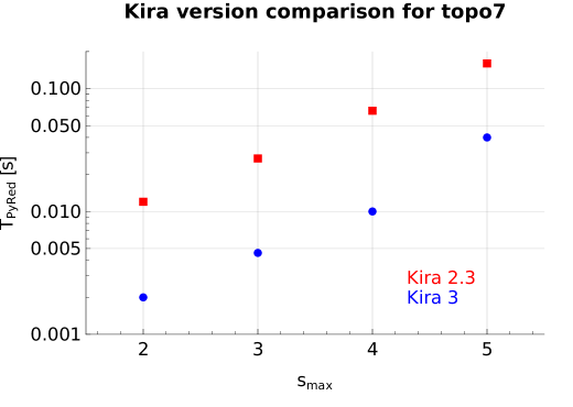
Figure 4: Scaling of the solution time $T_{\texttt{pyRed}{}}$ for the planar double-box topo7 with Kira 3 and Kira 2.3.

Compared to Kira 2.3, Kira 3 can solve the system with $s_{\mathrm{max}}+2$ in the same time, highlighting the improvements in the new version. Overall, the improvements for these trivial examples are certainly welcome, but only the more complicated examples in the following subsections show the true power of the new version.

5.2 Tennis-court topology

As the first non-trivial example we study the three-loop TennisCourt topology depicted in Fig.˜3(c). In Table˜4 we show the reductions for Kira 2.3 and Kira 3 at the same complexity with $r_{\mathrm{max}}=10$, $s_{\mathrm{max}}=3$, and $d_{\mathrm{max}}=0$.

Table 4: The reductions are performed with different integral complexities for the three-loop integral family TennisCourt. The number of master integrals is 166.

problem	r.s.d	10.3.0		10.4.0	10.5.0	10.6.0	10.7.0
	version	Kira 2.3	Kira 3
	truncate_sp	-	l=7	l=6	l=5	l=4	l=3
generation	# gen.	8 272 762	387 011	865 442	2 984 878	9 734 618	27 999 684
	# indep.	4 890 067	282 686	603 856	1 827 965	5 253 869	13 555 275
	# sel.	2 768 144	115 021	333 055	1 034 357	2 900 250	7 259 008
	RAM [GiB]	35.44	0.56	1.62	5.05	15.61	46.18
	$T_{\mathrm{gen}}$ [min:s]	41:36.3	0:28.7	1:09.4	3:23.0	11:43.8	46:30.2
FF	$T_{\texttt{pyRed}{}}$ [s]	146	0.91	4.16	15.3	63	212

Kira 3 generates about 21 times less equations and selects a system with about 24 times less equations. This means that in this case the ratio of selected equations to generated equations drops slightly from 33 % to 30 %, staying on a acceptable level. Furthermore, it requires about 63 times less main memory to set up the system and is about 87 times faster in doing so. Finally, we see a performance improvement of a factor 160 in the reduction time on a finite field point. To give glimpse what is now possible, we also show more complicated reductions by increasing $s_{\mathrm{max}}$ up to seven for Kira 3. The tremendous effect is visualized in Fig.˜5 where a reduction of integrals with seven numerators with Kira 3 is as efficient as a reduction of integrals with three numerators with Kira 2.3.

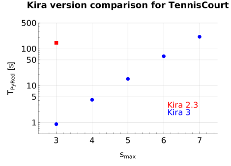
Figure 5: Scaling of the solution time $T_{\texttt{pyRed}{}}$ for the TennisCourt topology with Kira 2.3 and Kira 3.

5.3 Double-pentagon and pentagon-hexagon topologies

In Table˜5 we study the integral family doublePentagon depicted in Fig.˜3(d).

Table 5: Comparison of Kira 2.3 and Kira 3 for the integral family doublePentagon. Both reduce to 108 master integrals.

problem	r.s.d	8.5.0		9.5.1	13.5.5
	version	Kira 2.3	Kira 3
	truncate_sp	-	l=4	l=4	l=4
generation	# gen.	16 872 564	73 902	485 560	29 942 304
	# indep.	4 842 650	53 648	234 344	7 517 845
	# sel.	1 157 381	41 998	147 756	2 895 663
	RAM [GiB]	25.04	0.34	1.08	35.17
	$T_{\mathrm{gen}}$ [min:s]	33:46.0	0:08.8	0:45.8	44:46.6
FF	$T_{\texttt{pyRed}{}}$ [s]	33.0	1.3	4.0	122.0

We find a significant improvement of the new version Kira 3 compared to the previous version Kira 2.3 in all metrics: Kira 3 generates 228 times less equations and selects 28 times less equations. The ratio of independent equations to generated equations improves from 29 % to 73 % and the ratio of selected equations to generated equations from 6.9 % to 57 %, again highlighting that many irrelevant equations are no longer generated. This translates to a reduction in main memory requirements by a factor of 74 and improves the runtime by a factor of 107. Finally, the solution time for a phase space point over a finite field improves by a factor of 25. In addition we demonstrate that Kira 3 is also efficient when we include dots in addition to numerators. Even the extreme case of five dots in the top-level sector is only of slightly higher complexity than the reduction without dots with Kira 2.3.

Due to their importance for phenomenology, two-loop $2\to 3$ topologies have been studied extensively over the last decade and many ideas for efficient reductions have been developed. We also tried the doublePentagon topology with two of those dedicated and more involved strategies: the block triangular form [56, 58] as implemented in Blade [17] and syzygy equations [18, 19, 20, 21, 22, 23, 24, 25, 26] as implemented in NeatIBP [27, 28]. For the latter, we also tried the spanning cuts (spc.) strategy recently implemented in its latest version 1.1. For the block triangular system we take the system provided in Ref. [58] and improved all of the coefficients with Horner’s method. Since we cannot compare the methods themselves properly with one single example, we did not necessarily tune the other methods to achieve their best performance. Nonetheless, the corresponding measurements in Table˜6 allow us to make some interesting preliminary observations.

Table 6: Different strategies applied to the doublePentagon topology shown in Fig.˜3(d) at the complexity 8.5.0. The numbers for syzygies with spanning cuts are summed over all cuts.

	Kira 3	syzygies	syzygies (spc.)	block triangular
$T_{\mathrm{gen}}$	8.8 s	$\sim$ hours	$\sim$ hours	$\sim$ hours
# equations	41 998	26 106	23 834	3 497
# terms	734 833	1 498 728	544 355	388 973
disk [MiB]	3.7	46	8.6	23
$T_{\texttt{pyRed}}$ [s]	1.3	3.3	0.42	0.63
$T_{\texttt{Ratracer}{}}$ [s]	0.25	1.31	0.068	0.5

While in this example the system generated by Kira 3 contains more equations than the other systems, its equations consist of less terms on average and its size on disk in Kira readable format is actually smaller. This can be explained by the fact that Kira produces standard IBP equations with few terms and small algebraic coefficients, whereas the other strategies attempt to construct target oriented equations for the price of potentially longer equations and more complicated coefficients.

Despite these different characteristics, solving the systems with pyRed over finite fields results in comparable runtimes. Whereas solving the Kira system is completely dominated by the numerical Gaussian elimination, substituting numbers into the coefficients is non-negligible for the other systems.

In addition to Kira’s internal solver pyRed we also solved the systems with the external solver Ratracer [49], which records and plays the trace of operations and performs further optimizations. Again, we measure the time to solve the system for one phase space point over a finite field. Compared to pyRed, all systems benefit, but to a different degree. It is expected that different systems benefit from different solution strategies and solvers. However, we did not try any other solver for this manuscript. For example, Blade provides a solver specifically designed for the block triangular system [17].

As we have seen before, Kira 3 is able to generate the system in a few seconds, whereas the other methods take a few hours. In view of the many million, or even tens of million, sample points required for realistic applications, all of those generation times are typically negligible in the overall CPU budget. However, it could become relevant if the reduction coefficients are constrained with more sophisticated algorithms, see e.g. Refs. [86, 87, 48, 53, 88].

With the above, for this two-loop $2\to 3$ topology, Kira 3 now seems able to generate systems at a level of efficiency that was only achievable with dedicated strategies before. It will be interesting to study whether this observation holds for other topologies. For example, the three-loop $2\to 3$ topology studied in Ref. [89] was efficiently addressed by NeatIBP. Testing whether Kira 3 can reach the same level of efficiency is left for future explorations.

As a first glimpse in this direction, we study how Kira 3 scales with more complicated topologies for state-of-the-art calculations. In Table˜7 we first study the integral family doublePentagon when adding external and internal masses, see Figs.˜3(d), 3(e), 3(f) and 3(g).

Table 7: Kira 3’s performance for the more complicated double-pentagon topologies with external and internal masses from Figs.˜3(d), 3(e), 3(f) and 3(g) as well as the massless pentagon-hexagon topology shown in Fig.˜3(h).

problem	r.s.d	8.5.0 (doublePentagon, l=4)				9.5.0 (hex, l=5)
	topology	massless	one-mass	two-mass	internal mass	massless
	# masters	108	142	185	172	313
generation	# gen.	73 902	76 045	77 286	78 480	339 215
	# indep.	53 648	55 596	57 034	57 918	218 502
	# sel.	41 998	43 827	45 359	46 231	156 853
	RAM [GiB]	0.34	0.37	0.46	0.43	1.88
	$T_{\mathrm{gen}}$ [min:s]	0:08.8	0:09.9	0:12.8	0:11.6	1:10.0
FF	$T_{\texttt{pyRed}{}}$ [s]	1.35	1.6	2.5	2.1	16
	$T_{\texttt{Ratracer}{}}$ [s]	0.25	0.38	0.45	0.43	3.5

Even though these problems become significantly more complicated, be it in terms of the number of required sample points to obtain analytic reduction coefficients or the algebraic structure of the master integrals, there is only a mild increase in terms of main memory requirements and runtime when generating the system with Kira 3 and sampling it for individual phase space points. Only when adding an additional leg as in the topology hex depicted in Fig.˜3(h), there is a clear jump in complexity visible with Kira.

6 Conclusions

We presented the new version 3 of the Feynman integral reduction program Kira which brings enormous performance improvements and reductions of main memory requirements. This is mainly driven by a refined seeding strategy, generating significantly less equations while still being able to fully reduce the target integrals, and an improved equation selection algorithm. We quantified the performance improvements compared to Kira 2.3 at the hand of several different topologies at two- and three-loop order and observed for a single two-loop $2\to 3$ topology that the new version produces a system of equations on par with those generated by dedicated strategies.

Furthermore, we presented other new features such as the ability to add additional relations, sample the system numerically on chosen phase space points over finite fields, perform symbolic IBP reductions, and check the master integral basis.

We already applied this new version to a wide range of different projects, see Refs. [81, 73, 90, 74, 79], and believe that many more ambitious projects in both high-energy and gravitational-wave physics become now accessible with the public release of Kira 3. The source code is available on

https://gitlab.com/kira-pyred/kira

together with a more detailed changelog, installation instructions, and a wiki containing some best-practice guidelines. Bug reports and feature requests can be submitted via the issue system. In addition, a statically compiled version can be downloaded from

https://kira.hepforge.org/

While we have shown that the new seeding and selection strategies are vastly superior, further improvements seem realistic. On the one hand, we discussed in Section˜3.2 that the generated systems still contain irrelevant information which potentially could be filtered out with an improved selection algorithm, see e.g. Refs. [24, 27]. On the other hand, Refs. [62, 63, 64] recently introduced the concept of priority functions for seeding and applied machine learning techniques to find optimal distributions. Such an approach could address both seeding and selection and it will be interesting to investigate this in more detail in the future. In addition, new symmetry detection algorithms such as the one presented in Ref. [78] will allow us to uncover new relations between master integrals and could potentially lead to improved systems.

In this version we largely neglected the interpolation and reconstruction steps necessary to obtain analytic reduction coefficients. While for small rational functions with only a few variables those are typically limited by the sampling, for complicated rational functions the inherent costs of those algorithms become a bottleneck and the achieved performance improvements diminish. Thus, both technical and algorithmic improvements in FireFly might be necessary, e.g. following the ideas of Ref. [50, 53, 54, 55]. On the other hand it might be worthwhile to sample the phase space for $2\to 3$ and $2\to 4$ processes instead of interpolating the reduction tables, as for example pursued in Ref. [80]. As presented in Table˜7, the performance of the new version of Kira looks promising for this strategy. At the hand of Ratracer [49] we have seen that further speed ups are possible with technical improvements and better solution algorithms for linear systems, see also Refs. [51, 52]. It might also be worthwhile to study GPU acceleration.

For some applications a traditional algebraic solving strategy can still be advantageous. While Kira’s solver based on the computer algebra system Fermat already benefits from the improvements in this paper, further gains with other computer algebra systems seem possible [91, 9].

References

- [1] F. V. Tkachov, A Theorem on Analytical Calculability of Four Loop Renormalization Group Functions, Phys. Lett. B 100 (1981) 65.
- [2] K. Chetyrkin and F. Tkachov, Integration by parts: The algorithm to calculate functions in 4 loops, Nucl. Phys. B192 (1981) 159.
- [3] S. Laporta, High precision calculation of multiloop Feynman integrals by difference equations, Int. J. Mod. Phys. A 15 (2000) 5087 [hep-ph/0102033].
- [4] C. Anastasiou and A. Lazopoulos, Automatic integral reduction for higher order perturbative calculations, JHEP 07 (2004) 046 [hep-ph/0404258].
- [5] A. V. Smirnov, Algorithm FIRE – Feynman Integral REduction, JHEP 10 (2008) 107 [0807.3243].
- [6] A. V. Smirnov and V. A. Smirnov, FIRE4, LiteRed and accompanying tools to solve integration by parts relations, Comput. Phys. Commun. 184 (2013) 2820 [1302.5885].
- [7] A. V. Smirnov, FIRE5: a C++ implementation of Feynman Integral REduction, Comput. Phys. Commun. 189 (2015) 182 [1408.2372].
- [8] A. V. Smirnov and F. S. Chuharev, FIRE6: Feynman Integral REduction with Modular Arithmetic, Comput. Phys. Commun. 247 (2020) 106877 [1901.07808].
- [9] A. V. Smirnov and M. Zeng, FIRE 6.5: Feynman integral reduction with new simplification library, Comput. Phys. Commun. 302 (2024) 109261 [2311.02370].
- [10] C. Studerus, Reduze – Feynman integral reduction in C++, Comput. Phys. Commun. 181 (2010) 1293 [0912.2546].
- [11] A. von Manteuffel and C. Studerus, Reduze 2 - Distributed Feynman Integral Reduction, 1201.4330.
- [12] P. Maierhöfer, J. Usovitsch and P. Uwer, Kira—A Feynman integral reduction program, Comput. Phys. Commun. 230 (2018) 99 [1705.05610].
- [13] J. Klappert, F. Lange, P. Maierhöfer and J. Usovitsch, Integral reduction with Kira 2.0 and finite field methods, Comput. Phys. Commun. 266 (2021) 108024 [2008.06494].
- [14] T. Peraro, FiniteFlow: multivariate functional reconstruction using finite fields and dataflow graphs, JHEP 07 (2019) 031 [1905.08019].
- [15] R. N. Lee, Presenting LiteRed: a tool for the Loop InTEgrals REDuction, 1212.2685.
- [16] R. N. Lee, LiteRed 1.4: a powerful tool for reduction of multiloop integrals, J. Phys. Conf. Ser. 523 (2014) 012059 [1310.1145].
- [17] X. Guan, X. Liu, Y.-Q. Ma and W.-H. Wu, Blade: A package for block-triangular form improved Feynman integrals decomposition, Comput. Phys. Commun. 310 (2025) 109538 [2405.14621].
- [18] J. Gluza, K. Kajda and D. A. Kosower, Towards a Basis for Planar Two-Loop Integrals, Phys. Rev. D 83 (2011) 045012 [1009.0472].
- [19] R. M. Schabinger, A New Algorithm For The Generation Of Unitarity-Compatible Integration By Parts Relations, JHEP 01 (2012) 077 [1111.4220].
- [20] H. Ita, Two-loop Integrand Decomposition into Master Integrals and Surface Terms, Phys. Rev. D 94 (2016) 116015 [1510.05626].
- [21] G. Chen, J. Liu, R. Xie, H. Zhang and Y. Zhou, Syzygies Probing Scattering Amplitudes, JHEP 09 (2016) 075 [1511.01058].
- [22] K. J. Larsen and Y. Zhang, Integration-by-parts reductions from unitarity cuts and algebraic geometry, Phys. Rev. D 93 (2016) 041701 [1511.01071].
- [23] J. Böhm, A. Georgoudis, K. J. Larsen, M. Schulze and Y. Zhang, Complete sets of logarithmic vector fields for integration-by-parts identities of Feynman integrals, Phys. Rev. D 98 (2018) 025023 [1712.09737].
- [24] J. Böhm, A. Georgoudis, K. J. Larsen, H. Schönemann and Y. Zhang, Complete integration-by-parts reductions of the non-planar hexagon-box via module intersections, JHEP 09 (2018) 024 [1805.01873].
- [25] D. Bendle, J. Böhm, W. Decker, A. Georgoudis, F.-J. Pfreundt, M. Rahn et al., Integration-by-parts reductions of Feynman integrals using Singular and GPI-Space, JHEP 02 (2020) 079 [1908.04301].
- [26] A. von Manteuffel, E. Panzer and R. M. Schabinger, Cusp and collinear anomalous dimensions in four-loop QCD from form factors, Phys. Rev. Lett. 124 (2020) 162001 [2002.04617].
- [27] Z. Wu, J. Boehm, R. Ma, H. Xu and Y. Zhang, NeatIBP 1.0, a package generating small-size integration-by-parts relations for Feynman integrals, Comput. Phys. Commun. 295 (2024) 108999 [2305.08783].
- [28] Z. Wu, J. Böhm, R. Ma, J. Usovitsch, Y. Xu and Y. Zhang, Performing integration-by-parts reductions using NeatIBP 1.1 + Kira, 2502.20778.
- [29] P. Mastrolia and S. Mizera, Feynman Integrals and Intersection Theory, JHEP 02 (2019) 139 [1810.03818].
- [30] H. Frellesvig, F. Gasparotto, S. Laporta, M. K. Mandal, P. Mastrolia, L. Mattiazzi et al., Decomposition of Feynman Integrals on the Maximal Cut by Intersection Numbers, JHEP 05 (2019) 153 [1901.11510].
- [31] H. Frellesvig, F. Gasparotto, M. K. Mandal, P. Mastrolia, L. Mattiazzi and S. Mizera, Vector Space of Feynman Integrals and Multivariate Intersection Numbers, Phys. Rev. Lett. 123 (2019) 201602 [1907.02000].
- [32] S. Weinzierl, On the computation of intersection numbers for twisted cocycles, J. Math. Phys. 62 (2021) 072301 [2002.01930].
- [33] H. Frellesvig, F. Gasparotto, S. Laporta, M. K. Mandal, P. Mastrolia, L. Mattiazzi et al., Decomposition of Feynman Integrals by Multivariate Intersection Numbers, JHEP 03 (2021) 027 [2008.04823].
- [34] V. Chestnov, F. Gasparotto, M. K. Mandal, P. Mastrolia, S. J. Matsubara-Heo, H. J. Munch et al., Macaulay matrix for Feynman integrals: linear relations and intersection numbers, JHEP 09 (2022) 187 [2204.12983].
- [35] V. Chestnov, H. Frellesvig, F. Gasparotto, M. K. Mandal and P. Mastrolia, Intersection numbers from higher-order partial differential equations, JHEP 06 (2023) 131 [2209.01997].
- [36] G. Fontana and T. Peraro, Reduction to master integrals via intersection numbers and polynomial expansions, JHEP 08 (2023) 175 [2304.14336].
- [37] G. Brunello, V. Chestnov, G. Crisanti, H. Frellesvig, M. K. Mandal and P. Mastrolia, Intersection numbers, polynomial division and relative cohomology, JHEP 09 (2024) 015 [2401.01897].
- [38] X. Jiang, M. Lian and L. L. Yang, Recursive structure of Baikov representations: The top-down reduction with intersection theory, Phys. Rev. D 109 (2024) 076020 [2312.03453].
- [39] G. Crisanti and S. Smith, Feynman integral reductions by intersection theory with orthogonal bases and closed formulae, JHEP 09 (2024) 018 [2405.18178].
- [40] G. Brunello, V. Chestnov and P. Mastrolia, Intersection Numbers from Companion Tensor Algebra, 2408.16668.
- [41] M. Lu, Z. Wang and L. L. Yang, Intersection theory, relative cohomology and the Feynman parametrization, JHEP 05 (2025) 158 [2411.05226].
- [42] M. Kauers, Fast Solvers for Dense Linear Systems, Nucl. Phys. B Proc. Suppl. 183 (2008) 245.
- [43] P. Kant, Finding linear dependencies in integration-by-parts equations: A Monte Carlo approach, Comput. Phys. Commun. 185 (2014) 1473 [1309.7287].
- [44] A. von Manteuffel and R. M. Schabinger, A novel approach to integration by parts reduction, Phys. Lett. B 744 (2015) 101 [1406.4513].
- [45] T. Peraro, Scattering amplitudes over finite fields and multivariate functional reconstruction, JHEP 12 (2016) 030 [1608.01902].
- [46] J. Klappert and F. Lange, Reconstructing rational functions with FireFly, Comput. Phys. Commun. 247 (2020) 106951 [1904.00009].
- [47] J. Klappert, S. Y. Klein and F. Lange, Interpolation of dense and sparse rational functions and other improvements in FireFly, Comput. Phys. Commun. 264 (2021) 107968 [2004.01463].
- [48] G. De Laurentis and B. Page, Ansätze for scattering amplitudes from p-adic numbers and algebraic geometry, JHEP 12 (2022) 140 [2203.04269].
- [49] V. Magerya, Rational Tracer: a Tool for Faster Rational Function Reconstruction, 2211.03572.
- [50] A. V. Belitsky, A. V. Smirnov and R. V. Yakovlev, Balancing act: Multivariate rational reconstruction for IBP, Nucl. Phys. B 993 (2023) 116253 [2303.02511].
- [51] X. Liu, Reconstruction of rational functions made simple, Phys. Lett. B 850 (2024) 138491 [2306.12262].
- [52] J. Mangan, FiniteFieldSolve: Exactly solving large linear systems in high-energy theory, Comput. Phys. Commun. 300 (2024) 109171 [2311.01671].
- [53] H. A. Chawdhry, p-adic reconstruction of rational functions in multiloop amplitudes, Phys. Rev. D 110 (2024) 056028 [2312.03672].
- [54] A. Maier, Scaling up to Multivariate Rational Function Reconstruction, 2409.08757.
- [55] A. Smirnov and M. Zeng, Feynman integral reduction: balanced reconstruction of sparse rational functions and implementation on supercomputers in a co-design approach, 2409.19099.
- [56] X. Liu and Y.-Q. Ma, Determining arbitrary Feynman integrals by vacuum integrals, Phys. Rev. D 99 (2019) 071501 [1801.10523].
- [57] Y. Wang, Z. Li and N. Ul Basat, Direct reduction of multiloop multiscale scattering amplitudes, Phys. Rev. D 101 (2020) 076023 [1901.09390].
- [58] X. Guan, X. Liu and Y.-Q. Ma, Complete reduction of integrals in two-loop five-light-parton scattering amplitudes, Chin. Phys. C 44 (2020) 093106 [1912.09294].
- [59] M. Barakat, R. Brüser, C. Fieker, T. Huber and J. Piclum, Feynman integral reduction using Gröbner bases, JHEP 05 (2023) 168 [2210.05347].
- [60] X. Guan, X. Li and Y.-Q. Ma, Exploring the linear space of Feynman integrals via generating functions, Phys. Rev. D 108 (2023) 034027 [2306.02927].
- [61] V. Chestnov, G. Fontana and T. Peraro, Reduction to master integrals and transverse integration identities, JHEP 03 (2025) 113 [2409.04783].
- [62] M. von Hippel and M. Wilhelm, Refining Integration-by-Parts Reduction of Feynman Integrals with Machine Learning, JHEP 05 (2025) 185 [2502.05121].
- [63] Z.-Y. Song, T.-Z. Yang, Q.-H. Cao, M.-x. Luo and H. X. Zhu, Explainable AI-assisted Optimization for Feynman Integral Reduction, 2502.09544.
- [64] M. Zeng, Reinforcement Learning and Metaheuristics for Feynman Integral Reduction, 2504.16045.
- [65] X. Liu and Y.-Q. Ma, AMFlow: A Mathematica package for Feynman integrals computation via auxiliary mass flow, Comput. Phys. Commun. 283 (2023) 108565 [2201.11669].
- [66] V. Shtabovenko, R. Mertig and F. Orellana, FeynCalc 10: Do multiloop integrals dream of computer codes?, Comput. Phys. Commun. 306 (2025) 109357 [2312.14089].
- [67] W. Chen, Semi-automatic calculations of multi-loop Feynman amplitudes with AmpRed, Comput. Phys. Commun. 312 (2025) 109607 [2408.06426].
- [68] R. M. Prisco, J. Ronca and F. Tramontano, LINE: Loop Integrals Numerical Evaluation, 2501.01943.
- [69] T. Gehrmann and E. Remiddi, Differential equations for two-loop four-point functions, Nucl. Phys. B 580 (2000) 485 [hep-ph/9912329].
- [70] A. Pak, The Toolbox of modern multi-loop calculations: novel analytic and semi-analytic techniques, J. Phys. Conf. Ser. 368 (2012) 012049 [1111.0868].
- [71] A. V. Smirnov and A. V. Petukhov, The Number of Master Integrals is Finite, Lett. Math. Phys. 97 (2011) 37 [1004.4199].
- [72] R. H. Lewis, Fermat, A Computer Algebra System for Polynomial and Matrix Computation, http://home.bway.net/lewis/.
- [73] M. Driesse, G. U. Jakobsen, G. Mogull, J. Plefka, B. Sauer and J. Usovitsch, Conservative Black Hole Scattering at Fifth Post-Minkowskian and First Self-Force Order, Phys. Rev. Lett. 132 (2024) 241402 [2403.07781].
- [74] M. Driesse, G. U. Jakobsen, A. Klemm, G. Mogull, C. Nega, J. Plefka et al., Emergence of Calabi–Yau manifolds in high-precision black-hole scattering, Nature 641 (2025) 603 [2411.11846].
- [75] Z. Bern, E. Herrmann, R. Roiban, M. S. Ruf, A. V. Smirnov, V. A. Smirnov et al., Amplitudes, supersymmetric black hole scattering at , and loop integration, JHEP 10 (2024) 023 [2406.01554].
- [76] S. Abreu, M. Becchetti, C. Duhr and M. A. Ozcelik, Two-loop master integrals for pseudo-scalar quarkonium and leptonium production and decay, JHEP 09 (2022) 194 [2206.03848].
- [77] F. Buccioni, P. A. Kreer, X. Liu and L. Tancredi, One loop QCD corrections to gg → at , JHEP 03 (2024) 093 [2312.10015].
- [78] Z. Wu and Y. Zhang, A new method for finding more symmetry relations of Feynman integrals, 2406.20016.
- [79] S. Abreu, P. F. Monni, B. Page and J. Usovitsch, Planar Six-Point Feynman Integrals for Four-Dimensional Gauge Theories, 2412.19884.
- [80] B. Agarwal, G. Heinrich, S. P. Jones, M. Kerner, S. Y. Klein, J. Lang et al., Two-loop amplitudes for production: the quark-initiated Nf-part, JHEP 05 (2024) 013 [2402.03301].
- [81] M. Fael and J. Usovitsch, Third order correction to semileptonic decay: Fermionic contributions, Phys. Rev. D 108 (2023) 114026 [2310.03685].
- [82] M. Fael, F. Lange, K. Schönwald and M. Steinhauser, A semi-analytic method to compute Feynman integrals applied to four-loop corrections to the -pole quark mass relation, JHEP 09 (2021) 152 [2106.05296].
- [83] P. Maierhöfer and J. Usovitsch, Kira 1.2 Release Notes, 1812.01491.
- [84] GNU Project, GCC, the GNU Compiler Collection, https://gcc.gnu.org/.
- [85] LLVM Developer Group, Clang: a C language family frontend for LLVM, https://clang.llvm.org/index.html.
- [86] S. Abreu, J. Dormans, F. Febres Cordero, H. Ita and B. Page, Analytic Form of Planar Two-Loop Five-Gluon Scattering Amplitudes in QCD, Phys. Rev. Lett. 122 (2019) 082002 [1812.04586].
- [87] S. Badger, C. Brønnum-Hansen, D. Chicherin, T. Gehrmann, H. B. Hartanto, J. Henn et al., Virtual QCD corrections to gluon-initiated diphoton plus jet production at hadron colliders, JHEP 11 (2021) 083 [2106.08664].
- [88] G. De Laurentis, H. Ita, B. Page and V. Sotnikov, Compact Two-Loop QCD Corrections for Production in Proton Collisions, 2503.10595.
- [89] Y. Liu, A. Matijašić, J. Miczajka, Y. Xu, Y. Xu and Y. Zhang, An Analytic Computation of Three-Loop Five-Point Feynman Integrals, 2411.18697.
- [90] M. Fael, T. Huber, F. Lange, J. Müller, K. Schönwald and M. Steinhauser, Heavy-to-light form factors to three loops, Phys. Rev. D 110 (2024) 056011 [2406.08182].
- [91] K. Mokrov, A. Smirnov and M. Zeng, Rational Function Simplification for Integration-by-Parts Reduction and Beyond, 2304.13418.
- [92] J. A. M. Vermaseren, Axodraw, Comput. Phys. Commun. 83 (1994) 45.
- [93] D. Binosi and L. Theußl, JaxoDraw: A Graphical user interface for drawing Feynman diagrams, Comput. Phys. Commun. 161 (2004) 76 [hep-ph/0309015].
- [94] R. V. Harlander, S. Y. Klein and M. Lipp, FeynGame, Comput. Phys. Commun. 256 (2020) 107465 [2003.00896].
- [95] R. Harlander, S. Y. Klein and M. C. Schaaf, FeynGame-2.1 – Feynman diagrams made easy, PoS EPS-HEP2023 (2024) 657 [2401.12778].