No Free Lunch: Non-Asymptotic Analysis
of Prediction-Powered Inference

Abstract

Prediction-Powered Inference (PPI) is a popular strategy for combining gold-standard and possibly noisy pseudo-labels to perform statistical estimation. Prior work has shown an asymptotic “free lunch” for PPI++, an adaptive form of PPI, showing that the asymptotic variance of PPI++ is always less than or equal to the variance obtained from using gold-standard labels alone. Notably, this result holds regardless of the quality of the pseudo-labels. In this work, we demystify this result by conducting an exact finite-sample analysis of the estimation error of PPI++ on the mean estimation problem. We give a “no free lunch” result, characterizing the settings (and sample sizes) where PPI++ has provably worse estimation error than using gold-standard labels alone. Specifically, PPI++ will outperform if and only if the correlation between pseudo- and gold-standard is above a certain level that depends on the number of labeled samples ($n$). In some cases our results simplify considerably: For Gaussian data, the correlation must be at least $1/\sqrt{n-2}$ in order to see improvement, and a similar result holds for binary labels. In experiments, we illustrate that our theoretical findings hold on real-world datasets, and give insights into trade-offs between single-sample and sample-splitting variants of PPI++.

1 Introduction

Mean estimation is an ever-present problem: Medical researchers wish to understand the prevalence of disease, machine learning engineers want to understand the average performance of their models, and so on. Often, practioners have access to a large set of unlabeled examples, e.g., clinical notes that may or may not record the presence of a disease, images with unknown labels, etc. A typical approach to mean estimation is to gather (expensive) gold-standard labels for a small number of randomly selected examples, and take a simple average of the relevant metric across labeled cases.

In many scenarios, it is possible to construct cheap pseudo-labels using machine learning models or other heuristics. For instance, large language models (LLMs) and vision-language models (VLMs) can achieve reasonable “zero shot” performance on a variety of tasks (Radford et al., 2021). These pseudo-labels have the potential to improve estimation: For instance, if they were perfect substitutes for gold-standard labels, they would dramatically expand our sample size without introducing bias.

However, the quality of these pseudo-labels is often unknown a priori, and the naive approach of treating them as true standard labels can lead to erroneous conclusions. Prediction-Powered Inference (PPI) (Angelopoulos et al., 2023a) proposes an estimator that is unbiased for any set of pseudo-labels, by using the small labeled dataset (on which pseudo-labels can also be obtained) to estimate and correct for any pseudo-label bias. While PPI is unbiased, it is not guaranteed to improve variance / statistical efficiency, particularly when the pseudo-labels have weak correlation with the true labels. To this end, Angelopoulos et al. (2023b) proposed Power-Tuned PPI (PPI++), which uses the labeled dataset to infer the pseudo/true label correlation and discount the pseudo-labels if this correlation is small. Informed by analysis showing that the (asymptotic) variance of PPI++ is never greater than the variance of the classical estimator that only uses the labeled examples, they note (emphasis added)

[our] methods automatically adapt to the quality of available predictions, yielding easy-to-compute confidence sets…that always improve on classical intervals using only the labeled data. (Angelopoulos et al., 2023b)

However, this guarantee is asymptotic in nature, applying in the regime where the number of labeled examples becomes large, while the highest-value use of PPI++ comes precisely when labeled data is scarce. This leaves an open question: If the labeled sample is already too small to give a reliable estimate of the mean, when can we trust its assessment of the pseudo-labels?

We resolve this question by providing an exact expression for the finite-sample mean squared estimation error (MSE) of PPI++, which can be directly compared to the MSE of the classical estimator. For PPI++ with sample splitting (see Definition˜3.6), our analysis allows for any size of the labeled dataset and considers the unlabeled dataset to be arbitrarily large. Further, we place no restrictions on the joint distribution of pseudo- and true labels (other than bounded moments).

Our analysis produces a “no free lunch” result: PPI++ pays a price (in MSE terms) attributable to errors in estimating the correlation between pseudo- and true labels. If this correlation is small, then the costs of PPI++ outweigh the benefits. From our general results, we derive expressions for the minimum number of labeled samples that are required for PPI++ to improve upon the classical estimator. While our results apply to any distribution, they simplify considerably for Gaussian and binary labels. For Gaussian labels, the correlation must be larger than $(n-2)^{-1/2}$ for PPI++ to improve over the classical estimator, where $n$ is the labeled sample size.

PPI++ and variants are a useful tool, but require practitioners to implicitly assume that their pseudo-labels are “good enough”, a notion we define precisely in this work, enabling practitioners to make informed decisions. Our overall contributions can be summarized as follows:

• In Section˜4.1, we analyze PPI++ (with and without sample splitting) in the Gaussian setting, and provide interpretable bounds on the correlation/sample size required for PPI++ to outperform the classical estimator that uses only the labeled sample.

• In Sections˜4.2 and 4.3, we analyze PPI++ with sample splitting, for general distributions, showing that the same intuitions hold, and we provide an exact expression for the MSE in terms of moments of the joint pseudo/true label distribution.

• In Section˜4.4, we return to PPI++ without sample splitting, showing that this estimator has two undesirable properties for inference in finite samples: It is biased, and standard variance-estimation approaches can produce overly optimistic estimates of its variance.

• In Section˜5, we illustrate these findings empirically on real data, highlighting scenarios where PPI++ has worse MSE than the classical estimator, and demonstrating the tendency of PPI++ without sample splitting to produce overly narrow confidence intervals.

2 Related Work

The term “Prediction-Powered Inference” was coined by Angelopoulos et al. (2023a), who introduced the method in the context of both mean estimation and more general inference tasks. Recent work has proposed various extensions to PPI and PPI++, including their use with multiple estimands using additional shrinkage (Li and Ignatiadis, 2025), their use with cross-fitting of predictors (Zrnic and Candès, 2024b), and their use in the context of active statistical inference (Zrnic and Candès, 2024a). Others have proposed the use of PPI for application in clinical trials (Poulet et al., 2025), causal inference (Demirel et al., 2024), social science research (Broska et al., 2024), and the efficient evaluation of AI systems (Boyeau et al., 2024; Gligoric et al., 2025).

PPI shares substantial similarities with doubly-robust estimators in causal inference, as noted by Zrnic and Candès (2024a), and can be seen as a special case of the Augmented Inverse Propensity Weighted (AIPW) estimator (Bang and Robins, 2005). Through this lens, the unbiased nature of PPI (even when pseudo-labels are uninformative) is mirrored by the consistency of AIPW estimators under incorrect outcome-regression models. The core idea of PPI++ (taking linear combinations of unbiased estimators to minimize variance) dates back at least as far as Bates and Granger (1969). However, the theoretical analysis of these estimators is often limited to potentially loose non-asymptotic error bounds (Lavancier and Rochet, 2016) or study of their asymptotic efficiency. A distinct but related problem arises in the study of combining biased and unbiased estimators, where the bias of the former can be estimated from data. In that setting, a similar “no free lunch” phenomon has been observed, where these methods improve asymptotic variance for any fixed bias, but perform poorly when the bias is comparable in magnitude to $1/\sqrt{n}$ (Yang et al., 2023; Chen et al., 2021; Oberst et al., 2022). While our analysis strategy and problem setting differs substantially, our core result shows a conceptually similar point, that PPI++ tends to under-perform the classical estimator when the correlation between pseudo-labels and true labels is smaller than $\approx 1/\sqrt{n}$.

Despite the depth of literature on the topic of combining unbiased estimators, the characterization of the exact finite-sample variance (or mean squared estimation error) is often intractable outside of simple parameteric data-generating processes (e.g., Gaussian observations). For instance, in causal inference, one would require an exact understanding of the finite-sample behavior of the underlying propensity score or outcome-regression models. Our insight, in this context, is that this analysis becomes tractable precisely in the setting that motivates PPI++, where the model generating pseudo-labels is fixed, and an extremely large unlabeled dataset is available.

The theoretical characterization of PPI++ in other related work is largely limited to characterizing upper bounds on the benefits. Dorner et al. (2024) studies the limits of the benefits of PPI++, but focus on establishing upper bounds on the theoretical benefit, in the (optimistic) scenario where the optimal weight is chosen exactly. Likewise, (Chaganty et al., 2018), whose proposed method is largely identical to PPI++ in the mean estimation setting, do not consider the finite-sample behavior of their estimator beyond establishing that the bias is $O(1/n)$.

3 Setup: Mean Estimation with Pseudo-Labels

Notation: We use upper-case letters to denote a random variable (e.g., $Y$) and lower-case letters to denote a particular value (e.g., $y$). We use $P_{Y}$ to denote the distribution of a variable $Y$. We denote the mean of a random variable $Y$ by $\mu_{y}$, the variance by $\sigma_{y}^{2}$, and the covariance between two random variables $Y,X$ by $\sigma_{yx}$ or $\sigma_{xy}$. Given $n$ observations $\{x_{i},y_{i}\}_{i=1}^{n}$ of two random variables $X,Y$, the empirical covariance is given by $\hat{\sigma}_{xy}=\widehat{\text{Cov}}(X,Y)=\frac{1}{n-1}\sum_{i=1}^{n}(x_{i}-\bar{x}_{n})(y_{i}-\bar{y}_{n})$ where $\bar{x}_{n}$ and $\bar{y}_{n}$ are the sample means of $x$ and $y$ respectively over $n$ samples.

Problem Setting: We focus on the mean estimation problem: Our goal is to estimate the expectation of a variable (or “label”) $Y$, denoted $\theta\coloneqq\mathbb{E}[Y]$. We have access to a dataset of size $n$ (typically small), containing both covariates $X$ and true labels $Y$. Meanwhile, we have access to a dataset of size $N$ (typically much larger), which only contains unlabeled examples $X$. We make the standard assumption in this setting that both samples are drawn from a common distribution. This assumptions holds in the common scenario where a random subset of the entire dataset is chosen for labeling. To make use of the unlabeled data, we assume access to a model $f$ that can be queried to get pseudo-labels (or “synthetic labels”). The resulting pseudo-label on an input $X$ is given by $f(X)$, and we often write the pseudo-label as a variable $F\coloneqq f(X)$ where $f_{i}$ denotes a single sample of $F$. The classical estimator simply takes the average of the labeled examples to estimate the mean.

Definition 3.1 (Classical Estimator).

Let $\{y_{i}\}_{i=1}^{n}$ be $n$ samples drawn independently from $P_{Y}$, where the mean of $Y$ is given by $\theta\coloneqq\mathbb{E}[Y]$ and the variance by $\sigma^{2}_{y}\coloneqq\mathbb{E}[(Y-\theta)^{2}]$. The classical estimator of $\theta$ is the sample average $\hat{\theta}_{\text{Classical}}=\frac{1}{n}\sum_{i=1}^{n}y_{i}$ and is unbiased with variance $\sigma_{y}^{2}/n$.

Prediction Powered Inference: Prediction Powered Inference is a family of estimators that combine the labeled dataset of $n$ samples $\mathcal{D}_{n}=\{y_{i},f_{i}\}_{i=1}^{n}$ with the larger set of $N$ pseudo-label samples $\{f_{j}\}_{j=1}^{N}$. For mean estimation, the original  (Prediction Powered Inference (PPI) (Angelopoulos et al., 2023a)). estimator takes the following form.

Definition 3.2 (Prediction Powered Inference (PPI) (Angelopoulos et al., 2023a)).

Let $\mathcal{D}_{n}$ denote $n$ samples of $F,Y$ drawn from $P_{FY}$, and let $\mathcal{D}^{\prime}_{N}$ denote $N$ samples of $F$ drawn from $P_{F}$. The PPI estimator is then given by $\hat{\theta}_{\text{PPI}}=\frac{1}{n}\sum_{i\in\mathcal{D}_{n}}y_{i}+\frac{1}{N}\sum_{j\in\mathcal{D}^{\prime}_{N}}f_{j}-\frac{1}{n}\sum_{i\in\mathcal{D}_{n}}f_{i}$

Notice that  (Prediction Powered Inference (PPI) (Angelopoulos et al., 2023a)). (Definition˜3.2) is unbiased for any $f$. That is, $\mathbb{E}[\hat{\theta}_{\text{PPI++}}]=\mathbb{E}[Y]+\mathbb{E}[F]-\mathbb{E}[F]=\mathbb{E}[Y]$. However, the variance of  (Prediction Powered Inference (PPI) (Angelopoulos et al., 2023a)). depends on the variance of $Y-F$, which can be worse than the variance of $Y$ alone if $F$ is not sufficiently correlated with $Y$. Motivated by this concern, the  (Power Tuned PPI (PPI++) (Angelopoulos et al., 2023b)). estimator (Angelopoulos et al., 2023b) uses a data-driven parameter $\lambda$ to weight the contribution of the pseudo-labels. For mean estimation, the  (Power Tuned PPI (PPI++) (Angelopoulos et al., 2023b)). estimator takes the following form.

Definition 3.3 (Power Tuned PPI (PPI++) (Angelopoulos et al., 2023b)).

Let $\mathcal{D}_{n},\mathcal{D}^{\prime}_{N}$ be defined as in Definition˜3.2. The PPI++ estimator for mean estimation is then given by the following $\hat{\theta}_{\text{PPI++}}=\frac{1}{n}\sum_{i\in\mathcal{D}_{n}}y_{i}+\hat{\lambda}\left(\frac{1}{N}\sum_{j\in\mathcal{D}^{\prime}_{N}}f_{j}-\frac{1}{n}\sum_{i\in\mathcal{D}_{n}}f_{i}\right)$ with $\hat{\lambda}=\widehat{\text{Cov}}(Y,F)/((1+\frac{n}{N})\widehat{\text{Var}}(F))$

Note that if $\lambda=0$, then  (Power Tuned PPI (PPI++) (Angelopoulos et al., 2023b)). reduces to  (Classical Estimator)., and if $\lambda=1$, then  (Power Tuned PPI (PPI++) (Angelopoulos et al., 2023b)). reduces to  (Prediction Powered Inference (PPI) (Angelopoulos et al., 2023a)).. Angelopoulos et al. (2023b) note that the variance-optimal choice of $\lambda^{*}$ is given by $\lambda^{*}=(\sigma_{fy}/((1+\frac{n}{N})\sigma_{f}^{2})$, which motivates the “plug-in” estimator of $\hat{\lambda}$ above. We make two observations: First, the optimal value $\lambda^{*}$ increases with higher covariance between the pseudo-labels and the true labels ($\sigma_{fy}$), and with lower variance in the pseudo-labels ($\sigma_{f}^{2})$. Both quantities need to be estimated from data, but the covariance in particular needs to be estimated using labeled data: Notably, the true labels $Y$ are used for both (a) estimating the mean, and (b) estimating the quality of the pseudo-labels.

In many practical applications, the unlabeled sample size $N$ is extremely large, and in our work, we consider it to be effectively infinite, such that $\sigma_{f}^{2}$ and $\mu_{f}$ can be estimated with arbitrary precision, and the optimal tuning parameter $\lambda^{*}$ is given by $\sigma_{yf}/\sigma_{f}^{2}$. Notably, even when $N$ is infinite,  (Power Tuned PPI (PPI++) (Angelopoulos et al., 2023b)). still relies heavily on the small labeled sample of size $n$, which in practice may be very small. We now describe two variants of  (Power Tuned PPI (PPI++) (Angelopoulos et al., 2023b))., which vary in how they use the labeled data to obtain their estimate of the optimal $\lambda$. The first approach is to use the entire labeled sample for both (a) estimating $\hat{\lambda}$, and (b) estimating $\hat{\theta}$, which we refer to as  (Single-Sample PPI++, Infinite $N$)..

Definition 3.4 (Single-Sample PPI++, Infinite $N$).

Let $\mathcal{D}_{n}$ denote $n$ IID samples of $F,Y$ drawn from $P_{FY}$, and let $\mu_{f}$ denote the mean of $F$. Then the Single-Sample PPI++ estimate is given by

$$\hat{\theta}_{\text{Single-PPI++}} =\frac{1}{n}\sum_{i\in\mathcal{D}_{n}}y_{i}+\hat{\lambda}\left(\mu_{f}-\frac{1}{n}\sum_{i\in\mathcal{D}_{n}}f_{i}\right) \hat{\lambda} =\frac{\widehat{\text{Cov}}(Y,F;\mathcal{D}_{n})}{\sigma_{f}^{2}}$$

This estimator is simple, but the lack of sample splitting can complicate variance estimation and the construction of confidence intervals. For instance, as we show in Section˜4.4, when the same data is used to both (a) construct $\hat{\lambda}$, which minimizes the empirical variance, and (b) estimate the empirical variance while treating $\hat{\lambda}$ as fixed, then the resulting variance estimates can be overly optimistic.

To avoid this problem, one can use cross-fitting: splitting the labeled data and using one half to estimate $\lambda$ and the other to construct $\hat{\theta}$ (and estimate the variance) using the chosen $\hat{\lambda}$. This procedure is repeated by swapping the roles of each half (using the second half to estimate $\hat{\lambda}$, and the first to estimate $\hat{\theta}$), and the two estimates are averaged to produce a final estimate.

Definition 3.5 (Split-Sample PPI++ Estimator, infinite $N$).

Let $\mathcal{D}^{(1)}_{n},\mathcal{D}^{(2)}_{n}$ denote two independent sets of $n$ independent samples of $f(X),Y$ drawn from $P(X,Y)$. Let $\hat{\theta}^{(k)}$ denote the Split-Sample PPI++ Estimator using $\mathcal{D}^{(k)}_{n}$ to estimate $\hat{\lambda}$, and $\mathcal{D}^{(k^{\prime})}_{n}$ to estimate $\hat{\theta}$, where $k^{\prime}\neq k$, such that

$$\hat{\theta}^{(k)}_{\text{SS-PPI}} \coloneqq\frac{1}{n}\sum_{i\in\mathcal{D}^{(k^{\prime})}_{n}}y_{i}+\hat{\lambda}^{(k)}\left(\mu_{f}-\frac{1}{n}\sum_{i\in\mathcal{D}^{(k^{\prime})}_{n}}f(X_{i})\right) \hat{\lambda}^{(k)} \coloneqq\frac{\widehat{\text{Cov}}(f,Y;\mathcal{D}^{(k)}_{n})}{\sigma^{2}_{f}}$$

Definition 3.6 (Cross-fit PPI++ Estimator, infinite $N$).

Let $\mathcal{D}^{(1)}_{n},\mathcal{D}^{(2)}_{n}$ denote two independent sets of $n$ independent samples of $f(X),Y$ drawn from $P(X,Y)$. Let $\hat{\theta}^{(k)}$ denote the  (Split-Sample PPI++ Estimator, infinite $N$). Estimator, for $k=1,2$. The cross-fit PPI++ estimator is then given by $\hat{\theta}_{\text{CF-PPI++}}=(\hat{\theta}^{(1)}+\hat{\theta}^{(2)})/2$.

4 Theoretical Analysis

To understand relative performance of the classical and PPI++ estimators, we focus on their mean-squared estimation error, defined as $\mathsf{MSE}(\hat{\theta})\coloneqq\mathbb{E}[(\hat{\theta}-\theta)^{2}]$ for an estimator $\hat{\theta}$ and a target $\theta$. We focus on characterizing this error exactly in finite samples.

Our main results (Sections˜4.2 and 4.3) make no substantive assumptions regarding the distribution of $Y$ and $F$. That said, we begin in Section˜4.1 by analyzing a special case where labels and pseudo-labels are Gaussian, for which the analysis and the results are remarkably simpler. In this setting, the MSE of the  (Single-Sample PPI++, Infinite $N$). and  (Cross-fit PPI++ Estimator, infinite $N$). estimators are comparable and their behavior qualitatively similar to the more general results we derive later on.

In Section˜4.2, we move on to analyze the MSE of the  (Cross-fit PPI++ Estimator, infinite $N$). estimator for general distributions, showing that it depends primarily on the MSE of the individual  (Split-Sample PPI++ Estimator, infinite $N$). estimators, plus an additional positive term that captures dependence between folds. In particular, if the  (Split-Sample PPI++ Estimator, infinite $N$). estimator underperforms the  (Classical Estimator). estimator on $n$ samples, then the  (Cross-fit PPI++ Estimator, infinite $N$). estimator will underperform the  (Classical Estimator). estimator on $2n$ samples.

Motivated by this result, in Section˜4.3, we exactly characterize the MSE of the  (Split-Sample PPI++ Estimator, infinite $N$). estimator. In Section˜4.3, we decompose the MSE into three parts: The MSE of the classical estimator, a term that represents the gain in efficiency (i.e., a decrease in variance) attributable to pseudo-label quality, and a term that represents the loss in efficiency due to errors in estimating the quality of the pseudo-labels. In Section˜4.3.1, we first illustrate the relationship between these terms in the setting where pseudo-labels are completely random. Here, the MSE of  (Split-Sample PPI++ Estimator, infinite $N$). is always greater than the MSE of the classical estimator, by a multiplicative factor of $(1+(n-1)^{-1})$. In Section˜4.3.2, we characterize the MSE of the  (Split-Sample PPI++ Estimator, infinite $N$). estimator for any joint distribution of gold-standard and pseudo-labels. In Section˜4.3.3, we show how these results simplify in cases where labels are signed ($\{+1,-1\}$). Finally, in Section˜4.4, we return to discussion of the single-sample PPI++ estimator, which is more difficult to analyze theoretically, but has some unappealing properties from the perspective of confidence interval construction: It is biased in finite samples, and estimates of the variance that treat $\lambda$ as fixed can lead to misleading optimism. We provide full formal proofs for all theoretical results in Appendix˜A

4.1 Warm Up: Gaussian Labels

We begin with the special case where $Y$ and $F$ are normally distributed, for two reasons. First, this special case allows for a unified analysis of both the  (Single-Sample PPI++, Infinite $N$). and the  (Cross-fit PPI++ Estimator, infinite $N$). estimators, and establishes the existence of settings where both estimators under-perform (Classical Estimator).. Second, this special case provides simple expressions for the $\mathsf{MSE}$ of each estimator that capture the fundamental “no free lunch” nature of the problem.

[Condition for $\mathsf{MSE}$ Improvement, Gaussian Case]propositionMSESingleSampleNormal Let $Y,F$ be jointly Gaussian random variables, and consider the (Single-Sample PPI++, Infinite $N$). and  (Cross-fit PPI++ Estimator, infinite $N$). estimators which both make use of $2n$ labeled samples overall. Then,

$$\mathsf{MSE}(\hat{\theta}_{\text{PPI++}}) <\mathsf{MSE}(\hat{\theta}_{\text{Classical}}) \iff \frac{1}{\sqrt{c\cdot n-2}} <\left|\frac{\sigma_{fy}}{\sigma_{y}\sigma_{f}}\right|$$

where $c=2$ for  (Single-Sample PPI++, Infinite $N$). and $c=1$ for  (Cross-fit PPI++ Estimator, infinite $N$).. Note that if the reverse inequality holds, the $\mathsf{MSE}$ of each estimator is higher than that of (Classical Estimator).. Section˜4.1 provides a unifying perspective on the “no free lunch” phenomenon: If the correlation $\rho_{yf}\coloneqq\sigma_{fy}/(\sigma_{y}\sigma_{f})$ is non-zero, then pseudo-labels can improve our $\mathsf{MSE}$, but there is a minimum sample size at which this improvement kicks in. Notably, the condition for  (Cross-fit PPI++ Estimator, infinite $N$). uses $n$, the size of a single fold, while the condition for  (Single-Sample PPI++, Infinite $N$). uses $2n$, which illustrates one cost of sample splitting in this setting. However, if the correlation is zero, then both PPI++ estimators always performs worse than the classical estimator, as we show next. [$\mathsf{MSE}$, Independent Gaussian Case]propositionMSEIndependentNormal Let $Y,F$ be independent Gaussian random variables, and consider the (Single-Sample PPI++, Infinite $N$). and  (Cross-fit PPI++ Estimator, infinite $N$). estimators which both make use of $2n$ labeled samples overall. Then, the  (Single-Sample PPI++, Infinite $N$). and  (Cross-fit PPI++ Estimator, infinite $N$). estimators have $\mathsf{MSE}$ given by $\mathsf{MSE}(\hat{\theta}_{\text{PPI++}})=\mathsf{MSE}(\hat{\theta}_{\text{Classical}})\cdot\left(1+\frac{1}{(c\cdot n-1)}\right)$ where $c=2$ for  (Single-Sample PPI++, Infinite $N$). and $c=1$ for  (Cross-fit PPI++ Estimator, infinite $N$)..

If the covariance is zero, then $\lambda^{*}=0$, and this choice of $\lambda$ yields the same $\mathsf{MSE}$ as the classical estimator. In practice, however, $\hat{\lambda}$ is not exactly zero, leading to higher $\mathsf{MSE}$. As we will see in Section˜4.3.1, the same gap arises for  (Cross-fit PPI++ Estimator, infinite $N$). under general distributions, and we discuss the intuition further in Section˜4.3.1.

4.2 Performance of Cross-fit PPI++

We now proceed to focus on the finite sample $\mathsf{MSE}$ of  (Cross-fit PPI++ Estimator, infinite $N$). for general distributions. We omit a similar analysis of  (Single-Sample PPI++, Infinite $N$)., since the latter case is far less tractable to analyze, owing to complex dependencies that arise from estimating $\lambda$ on the same data used to form the final estimate. Our starting point is to relate the MSE of  (Cross-fit PPI++ Estimator, infinite $N$). to that of  (Split-Sample PPI++ Estimator, infinite $N$).. [MSE of Crossfit-PPI++]theoremCrossfitGeneralMSE Given a sample size of $2n$ labeled samples, the mean-squared error of the  (Cross-fit PPI++ Estimator, infinite $N$). estimator (Definition˜3.6) is given by

$$\mathsf{MSE}(\hat{\theta}_{\text{CF-PPI++}})=\frac{1}{2}\left[\mathsf{MSE}(\hat{\theta}_{\text{SS-PPI++}})+\frac{1}{n^{2}\sigma_{f}^{4}}(\sigma_{yf^{2}}-2\sigma_{fy}\mu_{f})^{2}\right]$$ (1)

where $\hat{\theta}_{\text{SS-PPI++}}$ is the  (Split-Sample PPI++ Estimator, infinite $N$). estimator (Definition˜3.5). Section˜4.2 demonstrates that the  (Cross-fit PPI++ Estimator, infinite $N$). estimator, by reusing both folds of the data, achieves slightly more than half the MSE of using a single fold. Note that $\theta_{\text{SS-PPI++}}$ (and hence, $\theta_{\text{CF-PPI++}}$) is unbiased, and as we will see in Section˜4.3, the MSE (i.e., the variance) of $\theta_{\text{SS-PPI++}}$ is $O(1/n)$. The final term in Equation˜1 is $O(1/n^{2})$, and so vanishes asymptotically relative to the MSE of the  (Split-Sample PPI++ Estimator, infinite $N$). estimator, but in finite samples represents extra variance due to dependence between the two estimates used in the  (Cross-fit PPI++ Estimator, infinite $N$). estimator. This result has important implications for analyzing when  (Cross-fit PPI++ Estimator, infinite $N$). outpeforms the classical estimator, which motivates our investigation next of the  (Split-Sample PPI++ Estimator, infinite $N$). estimator.

[Sufficient Condition for Worse Performance]corollaryConditionCrossFitWorse If $\mathsf{MSE}(\hat{\theta}_{\text{SS-PPI++}})>\sigma_{y}^{2}/n$, then the  (Cross-fit PPI++ Estimator, infinite $N$). estimator has higher MSE (i.e., higher variance) than the classical estimator.

4.3 Theoretical Analysis of Split-Sample PPI++

We now proceed to analyze the (Split-Sample PPI++ Estimator, infinite $N$). estimator defined in Definition˜3.5. Our first result characterizes the relative efficiency to the classical estimator. Motivated by Section˜4.2, we compare the performance of  (Split-Sample PPI++ Estimator, infinite $N$). to that of the classical estimator using $n$ samples. [Relative MSE of Split-Sample PPI++ versus the Classical Estimator]theoremGeneralMSE The  (Split-Sample PPI++ Estimator, infinite $N$). estimator given in Definition˜3.5, which estimates $\hat{\lambda}$ using $n$ samples, and uses an independent sample of size $n$ to estimate $\theta$, has MSE given by

$$\mathsf{MSE}(\hat{\theta}_{\text{SS-PPI++}})=\underbrace{\frac{\sigma_{y}^{2}}{n}}_{\text{Var}(\bar{y}_{n})}-\underbrace{\frac{\sigma_{fy}^{2}}{n\sigma_{f}^{2}}}_{\text{(Eff. Gain)}}+\underbrace{\frac{1}{n\sigma_{f}^{2}}\mathbb{E}[(\hat{\sigma}_{fy}-\sigma_{fy})^{2}]}_{\text{(Eff. Loss)}}$$ (2)

where the first term (Eff. Gain) captures the gain in efficiency from using a predictor $f$ that is highly correlated with the true label $Y$, and the second term (Eff. Loss) captures the loss of efficiency that arises from errors in estimating the covariance from data. In Section˜4.3.2 we will characterize the last term in Equation˜2, which can be combined with Sections˜4.3 and 4.2 to give the exact MSE of the  (Cross-fit PPI++ Estimator, infinite $N$). estimator. For now, we note that Equation˜2 gives a necessary and sufficient condition for  (Split-Sample PPI++ Estimator, infinite $N$). to fail to provide benefits over using only labeled examples. [Condition for Worse Performance]corollaryConditionWorseSplit $\mathsf{MSE}(\hat{\theta}_{\text{SS-PPI++}})>(\sigma_{y}^{2}/n)$ if and only if $\mathbb{E}[(\hat{\sigma}_{fy}-\sigma_{fy})^{2}]>\sigma_{fy}^{2},$ i.e., if the $\mathsf{MSE}$ in covariance estimation is higher than the squared covariance. In other words, there is no free lunch, but rather an intuitive trade-off: If the error in estimating the covariance $\sigma_{fy}$ is higher than the magnitude of $\sigma_{fy}$, then  (Split-Sample PPI++ Estimator, infinite $N$). performs worse than simply using the $n$ labeled examples alone. Equations˜2 and 4.2 together imply that if this estimation error is too large, then  (Cross-fit PPI++ Estimator, infinite $N$). similarly under-performs the  (Classical Estimator). estimator.

In the following, we characterize the covariance estimation error $\mathbb{E}[(\hat{\sigma}_{fy}-\sigma_{fy})^{2}]$. To build intuition, we first revisit the setting where $Y,F$ are independent, and prove that the result in Footnote˜2 holds more generally in this setting. In Section˜4.3.2 we then give an explicit characterization (in Section˜4.3.2) of the covariance estimation error term.

4.3.1 Warm-up: Performance Gap with Random Pseudo-Labels

We revisit the case where $Y$ and $F$ are independent, but now allow for non-Gaussian distributions. propositionIndependentMSE Given $2n$ samples $\{y_{i},f_{i}\}_{i=1}^{n}$ drawn from $P_{FY}$, where $Y$ and $F$ are independent with bounded second moments, the MSE of  (Split-Sample PPI++ Estimator, infinite $N$). and  (Cross-fit PPI++ Estimator, infinite $N$). are given by

$$\mathsf{MSE}(\hat{\theta}_{\text{SS-PPI++}}) =\frac{\sigma^{2}_{y}}{n}\left(1+\frac{1}{n-1}\right) \mathsf{MSE}(\hat{\theta}_{\text{CF-PPI++}}) =\frac{\sigma^{2}_{y}}{2n}\left(1+\frac{1}{n-1}\right)$$ and

Note that in the setting of Section˜4.3.1, the $\mathsf{MSE}$ of the  (Classical Estimator). estimator is $\sigma^{2}_{y}/2n$. Section˜4.3.1 can help build intuition that bridges the non-asymptotic and asymptotic regimes. Since  (Split-Sample PPI++ Estimator, infinite $N$). and  (Cross-fit PPI++ Estimator, infinite $N$). are unbiased, their $\mathsf{MSE}$ is equal to their variance. Accordingly, in the setting of independent pseudo-labels, the finite-sample variance of these PPI++ estimators is always greater than the variance of the classical estimator, even if the asymptotic variance is identical.

4.3.2 Finite-Sample Covariance Estimation Error with General Pseudo-Labels

Before introducing our main result, we introduce additional notation regarding the covariance and variance of higher powers. For two variables (e.g., $F$ and $Y$) and two integers $a,b$, we use $\sigma_{f^{a}y^{b}}$ to refer to the covariance between the random variable $F^{a}$ and the random variable $Y^{b}$. For a single variable $Y$, we similarly use $\sigma^{2}_{Y^{a}}$ to denote the variance of $Y^{a}$. We now present a full treatment of the covariance estimation error for general distributions. [Covariance Estimation Error, General Case]theoremGeneralCovarianceEstimation Let $Y$ and $F$ have bounded fourth-moments. Given $n$ samples $\{y_{i},f_{i}\}_{i=1}^{n}$ from the joint distribution of $Y$ and $F$, we have

$$\mathbb{E}[(\hat{\sigma}_{yf}-\sigma_{yf})^{2}]=\frac{1}{n}\sigma_{f^{2}y^{2}}+\frac{1}{n-1}\sigma_{f}^{2}\sigma_{y}^{2}-\frac{(n-2)}{n(n-1)}\sigma_{fy}^{2}-\frac{2}{n}[\sigma_{y^{2}f}\mu_{f}+\sigma_{f^{2}y}\mu_{y}-2\sigma_{fy}\mu_{f}\mu_{y}]$$

Combining Section˜4.3.2 with Equation˜2 characterizes the scenarios where  (Split-Sample PPI++ Estimator, infinite $N$). out-performs  (Classical Estimator).. While the exact characterization involves several terms, we will demonstrate cases below where it simplifies substantially. To build intuition, note that the condition in Equation˜2 is equivalent to the condition (dividing both sides by $\sigma_{y}^{2}\sigma_{f}^{2}$) that $\mathbb{E}[(\hat{\sigma}_{yf}-\sigma_{yf})^{2}]/\sigma_{y}^{2}\sigma_{f}^{2}>\sigma_{yf}^{2}/\sigma_{y}^{2}\sigma_{f}^{2}=\rho_{fy}^{2}$, where the left-hand side is $O(1/n)$. Hence, as long as the correlation $\rho_{fy}$ is non-zero, there exists a sample size $n$ such that the  (Split-Sample PPI++ Estimator, infinite $N$). estimator out-performs using the labeled data alone, but below this required sample size, it will generally perform worse.

4.3.3 Example: Binary Labels

For signed binary labels taking values in $\{-1,1\}$, the bounds simplify considerably, because $F^{2}=Y^{2}=1$, such so the higher order covariance terms (e.g., $\sigma_{y^{2}f},\sigma_{y^{2}f^{2}}$, etc.) vanish. [Signed Binary Labels]propositionBinaryPPI Under the conditions of Section˜4.3.2, if $F,Y$ take values in $\{-1,+1\}$, the MSE of the  (Split-Sample PPI++ Estimator, infinite $N$). estimator is less than $(\sigma_{y}^{2}/n)$ if

$$\sqrt{\frac{n}{(n^{2}-2)}+A_{n}(f,y)^{2}}-\left|A_{n}(f,y)\right| <\left|\frac{\sigma_{yf}}{\sigma_{f}\sigma_{y}}\right| A_{n}(f,y) \coloneqq\frac{2(n-1)}{n^{2}-2}\frac{\mu_{f}\mu_{y}}{\sigma_{f}\sigma_{y}}$$ where (3)

Note that the left-hand side of Equation˜3 is $O(1/\sqrt{n})$, since $A_{n}=O(1/n)$, recovering similar qualitative behavior to the Gaussian case.

4.4 Bias and Variance Estimate of Single-Sample PPI++

In addition to mean squared error, practitioners conducting statistical inference are often concerned with the construction of confidence intervals. Typically, we construct asymptotically valid confidence intervals using the variance of a consistent estimator, and hence lower variance yields tighter intervals. While such intervals are generally not guaranteed to maintain nominal coverage in finite samples, (Single-Sample PPI++, Infinite $N$). introduces two additional challenges. First, it is biased in finite sample, and second, it can produce overly optimistic variance estimates. We first characterize the exact bias in Footnote˜4, and in Section˜4.4 we illustrate that under mild conditions, standard methods for estimating the variance of  (Single-Sample PPI++, Infinite $N$). will necessarily yield estimates that are lower than the classical variance, even in scenarios (as illustrated in Section˜4.1) where we know the MSE of  (Single-Sample PPI++, Infinite $N$). is higher than that of the classical estimator. [Bias of Single Sample]propositionBiasSingleSample The bias of the  (Single-Sample PPI++, Infinite $N$). defined in Definition˜3.4 is given by $\mathbb{E}[\hat{\theta}_{\text{Single-PPI++}}-\theta]=\left(2\sigma_{yf}\mu_{f}-\sigma_{yf^{2}}\right)/(n\sigma_{f}^{2})$

In Section˜4.4 we consider a variance estimation strategy that treats $\lambda$ as fixed, and uses plug-in estimators to estimate each component of the variance (namely, $\hat{\sigma}_{y},\hat{\sigma}_{f},$ and $\hat{\sigma}_{yf}$). In the appendix, we present a similar result for another common method of variance estimation, that similarly treats the estimated $\lambda$ as fixed, and uses the empirical variance of $y-\lambda f$ in $\mathcal{D}_{n}$ and $\lambda f$ in $\mathcal{D}^{\prime}_{N}$.

[Optimistic Variance Estimation of Single Sample PPI++]propositionOptimisticVarianceSSPPI Consider the variance estimator for  (Single-Sample PPI++, Infinite $N$). given by $\hat{\sigma}^{2}_{\text{Single-PPI++}}=(1/n)[\hat{\sigma}^{2}_{y}+\lambda^{2}\sigma^{2}_{f}-2\lambda\hat{\sigma}_{fy}]$. This estimate reduces to $(1/n)[\hat{\sigma}^{2}_{y}-\hat{\sigma}^{2}_{fy}/\sigma^{2}_{f}]$, which is always less than the classical plug-in variance $\hat{\sigma}^{2}_{y}/n$. As a result of Section˜4.4, the asymptotic confidence intervals constructed for  (Single-Sample PPI++, Infinite $N$). will always be narrower than those of  (Classical Estimator)., even if the true variance is larger. In Section˜5, we show empirically that these always tighter intervals can result in significant drops in coverage.

5 Experiments

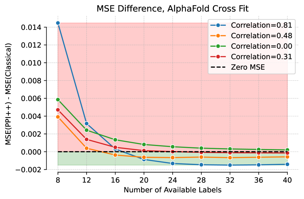
(a) Cross-fit PPI++ Estimator

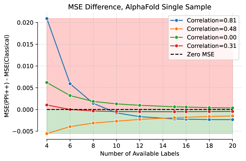
(b) Single-Sample PPI++ Estimator

Figure 1: Relative $\mathsf{MSE}$ vs. Sample Size on the Alphafold Dataset for PPI++ estimators with black-box models $f$ of varying quality. Y-axis gives the difference $\mathsf{MSE}(\hat{\theta}_{\text{PPI++}})-\mathsf{MSE}(\hat{\theta}_{\text{Classical}})$, such that lower (negative) values imply improvement over the classical estimator. Each line represents PPI++ with a different black-box model $f$. The blue line uses the original model, which has strong predictive performance, but only improves estimation error at $2n\geq 20$ (left) and $n\geq 10$ (right).

In this section, we illustrate the implications of our theory with experiments on the Alphafold (Jumper et al., 2021) dataset used in Angelopoulos et al. (2023b), using a similar experimental setup where we use bootstrapping to simulate multiple draws from a common distribution, and use the empirical mean of the (larger) original dataset set for establishing ground truth. Note that we focus on the low sample size regime where n < 50. See Appendix˜B for more details. See Appendix˜C for additional results on the galaxies (Angelopoulos et al., 2023b) dataset.

In Figure˜1, we show the relative MSE of PPI++ as a function of labeled dataset size $n$, which gives results that are in line with our theoretical developments for  (Cross-fit PPI++ Estimator, infinite $N$)., and which illustrate that similar trends hold for  (Single-Sample PPI++, Infinite $N$).. In particular, using pseudo-labels with varying quality, the MSE either (a) starts off worse than classical, but starts to improve over classical past a certain ‘tipping point’ sample size, (b) starts off worse than classical, but closes the gap as dataset size increases, or (c) starts off better than classical and stays there. We note that for the pseudo-label models shown here,  (Single-Sample PPI++, Infinite $N$). tends to achieve lower $\mathsf{MSE}$ than  (Cross-fit PPI++ Estimator, infinite $N$)..

In Figure˜2, we show the coverage and average widths of intervals constructed via (Single-Sample PPI++, Infinite $N$). and (Cross-fit PPI++ Estimator, infinite $N$).. We note that the (Single-Sample PPI++, Infinite $N$). method produces intervals that are narrower than those from the (Classical Estimator). (right). However, these substantively tighter intervals come at the cost of inadequate coverage (left). Comparing Figures˜2(a) and 2(b), both (Single-Sample PPI++, Infinite $N$). and (Cross-fit PPI++ Estimator, infinite $N$). show wider intervals as the correlation drops, and while (Cross-fit PPI++ Estimator, infinite $N$). widens enough to match the coverage of (Classical Estimator)., (Single-Sample PPI++, Infinite $N$). still falls short in this regard.

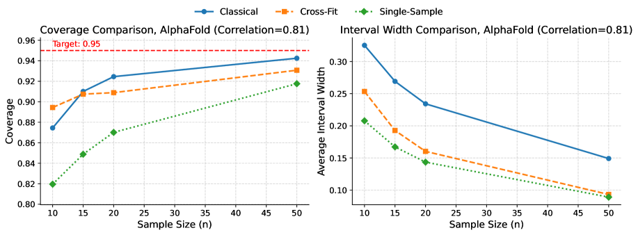
(a)

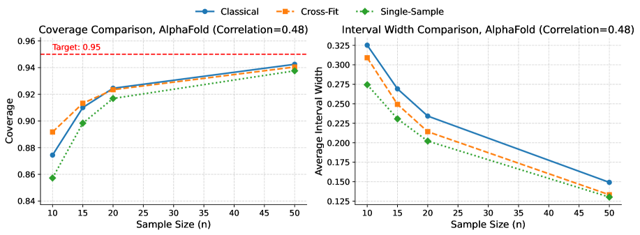
(b)

Figure 2: Comparison of Coverage and Interval Width for  (Cross-fit PPI++ Estimator, infinite $N$). and  (Single-Sample PPI++, Infinite $N$)., using different models $f$ on the Alphafold dataset. (2(a)) Original pseudo-label model $f$, where Single-Sample PPI++ has substantially lower coverage than either Cross-fit PPI++ or the classical estimator. (2(b)) A modified model with lower correlation, where similar trends hold.

6 Conclusions

Intuitively, there is no “free lunch” when it comes to using predictions in statistical inference, and we have shown this formally in the case of PPI++. Importantly, beyond establishing a no-free-lunch result, this paper provides a clear analysis that precisely characterizes when we should expect PPI++ to perform well, offering practical guidance to practitioners. Using our expression for the MSE of the  (Cross-fit PPI++ Estimator, infinite $N$). variant of PPI++, practioners can use their prior knowledge of (or assumptions on) the quality of the pseudo-labels, to assess whether they are in the regime where PPI++ should improve statistical efficiency. Our hope is that these results will be useful to practitioners when deciding how much labeled data is required to see a benefit from PPI++, and to help justify the use of PPI++ and related methods more formally in applications.

Supplementary Material

Appendix A Proofs

Here we include full formal proofs for all the theoretical results in our paper. We provide a table of contents for ease of navigation. The organization is as follows:

We start with the proof of the $\mathsf{MSE}$ of the (Cross-fit PPI++ Estimator, infinite $N$). estimator, showing that it is composed of the $\mathsf{MSE}$ of the (Split-Sample PPI++ Estimator, infinite $N$). and variance introduced by dependence between the folds of the cross-fit. A natural transition then is to characterize the $\mathsf{MSE}$ of the (Split-Sample PPI++ Estimator, infinite $N$). estimator. We derive the $\mathsf{MSE}$ of this estimator in terms of the covariance estimation error. Then we characterize this error, warming-up in the case of independent pseudo-labels before presenting a full general treatment. We follow this with a derivation of the error and $\mathsf{MSE}$ condition for the special case of signed binary variables. We are then ready to present a proof of the unified $\mathsf{MSE}$ analysis in the Gaussian case for (Single-Sample PPI++, Infinite $N$). and (Cross-fit PPI++ Estimator, infinite $N$).. Then, we change tracks from $\mathsf{MSE}$ to provide a proof of the bias of the (Single-Sample PPI++, Infinite $N$). estimator and its empirical variance estimate.

A.1 Foreword and Useful Lemmas

Remark A.1 (Use of subscripts).

We often make use of subscripts $y_{i},f_{j}$, etc in two contexts: First, we use these subscripts in the standard context as part of a sum. For instance, we may write $\mathbb{E}[\bar{y}\bar{f}]=\frac{1}{n}\sum_{i=1}^{n}\mathbb{E}[y_{i}\bar{f}]$. Second, we use these subscripts as short-hand to distinguish between variables corresponding to different samples. Continuing the previous example, we may write $\mathbb{E}[\bar{y}\bar{f}]=\frac{1}{n}\sum_{i=1}^{n}\mathbb{E}[y_{i}\bar{f}]=\frac{1}{n}n\cdot\mathbb{E}[y_{i}\bar{f}]$. Here, we make implicit use of the fact that for any $i\in\{1,\ldots,n\}$, the expectation $\mathbb{E}[y_{i}\bar{f}]$ is identical by exchangeability. This notation is particularly useful when indicies differ. For instance $\mathbb{E}[y_{i}\bar{f}]=\frac{1}{n}\mathbb{E}[y_{i}(f_{i}+\sum_{j\neq i}f_{j})]=\frac{1}{n}\mathbb{E}[y_{i}f_{i}]+\frac{(n-1)}{n}\mathbb{E}[y_{i}f_{j}]$, where $\mathbb{E}[y_{i}f_{j}]$ denotes the expectation of $y_{i}$ (from some sample $i$) and $f_{j}$ (drawn from a distinct sample $j\neq i$), such that $\mathbb{E}[y_{i}f_{j}]=\mathbb{E}[y]\mathbb{E}[f]$ by independence, while $\mathbb{E}[y_{i}f_{i}]=\mathbb{E}[yf]$.

Lemma A.1 (Covariance Representation).

The empirical covariance can be equivalently written

$$\frac{1}{n-1}\sum_{i=1}^{n}(y_{i}-\bar{y})(f_{i}-\bar{f})=\frac{1}{n-1}\sum_{i=1}^{n}(y_{i}f_{i}-\bar{y}\bar{f})$$ (4)

Proof.

$$\frac{1}{n-1}\sum_{i=1}^{n}(y_{i}-\bar{y})(f_{i}-\bar{f}) =\frac{1}{n-1}\sum_{i=1}^{n}(y_{i}f_{i}-y_{i}\bar{f}-f_{i}\bar{y}+\bar{y}\bar{f})$$ (5)

and $\sum_{i}y_{i}\bar{f}=n\bar{y}\bar{f}=\sum_{i}\bar{y}\bar{f}$, and similarly with $f_{i}\bar{y}$. ∎

[Cross-term under Cross-Fitting]lemmaCrossTermExpectationGeneral Let $Y$ and $F$ be random variables with bounded second-moments. Suppose that we observe $n$ IID samples $\{y_{i},f_{i}\}_{i=1}^{n}$ from the joint distribution of $Y$ and $F$. Let $\bar{y}_{n},\bar{f}_{n}$ denote the sample means of $Y,F$ on the observed n-sample. Furthermore, let $\hat{\lambda}$ be independent of $\{y_{i},f_{i}\}_{i=1}^{n}$. Then we have,

$$\mathbb{E}\left[\hat{\lambda}(\bar{y}_{n}-\theta)(\mu_{f}-\bar{f}_{n})\right] =-\frac{\sigma_{yf}^{2}}{n\sigma_{f}^{2}}$$

Proof.

$$\mathbb{E}\left[\hat{\lambda}(\bar{y}_{n}-\theta)(\mu_{f}-\bar{f}_{n})\right]$$

$$=\mathbb{E}[\hat{\lambda}]\mathbb{E}[(\bar{y}_{n}-\theta)(\mu_{f}-\bar{f}_{n})] \hat{\lambda}$$ Independence of

$$=\mathbb{E}[\hat{\lambda}]\mathbb{E}\left[\bar{y}_{n}(\mu_{f}-\bar{f}_{n})-\theta(\mu_{f}-\bar{f}_{n})\right]$$

$$=\mathbb{E}[\hat{\lambda}]\mathbb{E}\left[\bar{y}_{n}(\mu_{f}-\bar{f}_{n})\right]-\mathbb{E}[\hat{\lambda}]\mathbb{E}\left[\theta(\mu_{f}-\bar{f}_{n})\right]$$ Linearity of Expectation

$$=\mathbb{E}[\hat{\lambda}]\mathbb{E}\left[\bar{y}_{n}(\mu_{f}-\bar{f}_{n})\right]-\mathbb{E}[\hat{\lambda}]\theta\mathbb{E}\left[(\mu_{f}-\bar{f}_{n})\right] \theta$$ is constant

$$=\mathbb{E}[\hat{\lambda}]\mathbb{E}\left[\bar{y}_{n}(\mu_{f}-\bar{f}_{n})\right]-\mathbb{E}[\hat{\lambda}]\theta(\mathbb{E}[\mu_{f}]-\mathbb{E}[\bar{f}_{n}])$$ Linearity of Expectation

Since $\mu_{f}=\mathbb{E}[\bar{f}_{n}]$, the second term vanishes. Further $\hat{\lambda}=\widehat{\text{Cov}}(Y,F)/\sigma^{2}_{f}$. where $\widehat{\text{Cov}}(Y,F)$ is an unbiased estimate of the covariance between $Y,F$. Therefore, $\mathbb{E}[\hat{\lambda}]=\frac{\sigma_{fy}}{\sigma^{2}_{f}}$. Plugging these in,

$$\mathbb{E}\left[\hat{\lambda}(\bar{y}_{n}-\theta)(\mu_{f}-\bar{f}_{n})\right] =\frac{\sigma_{fy}}{\sigma^{2}_{f}}\mathbb{E}\left[\bar{y}_{n}(\mu_{f}-\bar{f}_{n})\right]$$

$$=\frac{\sigma_{fy}}{\sigma^{2}_{f}}\left[\mathbb{E}[\bar{y}_{n}\mu_{f}]-\mathbb{E}[\bar{y}_{n}\bar{f}_{n}]\right]$$ Linearity of Expectation

Note that $\mathbb{E}[\bar{y}_{n}\mu_{f}]=\mu_{y}\mu_{f}$, and $\mathbb{E}[\bar{y}_{n}\bar{f}_{n}]$ can be written as

$$\mathbb{E}\left[\bar{y}_{n}\bar{f}_{n}\right] =\frac{1}{n^{2}}\mathbb{E}\left[\sum_{i}\sum_{j}y_{i}f_{j}\right]$$

$$=\frac{1}{n^{2}}\mathbb{E}\left[\sum_{i=j}y_{i}f_{j}+\sum_{i\neq j}y_{i}f_{j}\right]$$

$$=\frac{1}{n^{2}}(n\mathbb{E}[y_{i}f_{j}]+n(n-1)\mathbb{E}[y_{i}f_{j}])$$

$$=\frac{\sigma_{yf}}{n}+\frac{n}{n^{2}}\mu_{f}\mu_{y}+\frac{n(n-1)}{n^{2}}\mu_{f}\mu_{y}$$

$$=\frac{\sigma_{fy}}{n}+\mu_{f}\mu_{y}$$

Where we have used the fact that in the expansion of $\bar{y}\bar{f}$, there are $n$ terms where $i=j$, such that $E[y_{i}f_{j}i=\sigma_{fy}+\mu_{f}\mu_{y}$ by definition of covariance, and there are $n(n-1)$ terms where $i\neq j$, such that $E[y_{i}f_{j}]=\mu_{f}\mu_{y}$, since $y_{i}\perp f_{j}$. Putting these together, we have

$$\mathbb{E}[\bar{y}_{n}\mu_{f}]-\mathbb{E}[\bar{y}_{n}\bar{f}_{n}]=\mu_{y}\mu_{f}-\frac{\sigma_{fy}}{n}-\mu_{f}\mu_{y}=-\frac{\sigma_{fy}}{n}$$

Therefore,

$$\mathbb{E}\left[\hat{\lambda}(\bar{y}_{n}-\theta)(\mu_{f}-\bar{f}_{n})\right]=\frac{\sigma_{fy}}{\sigma^{2}_{f}}\left[\mathbb{E}[\bar{y}_{n}\mu_{f}]-\mathbb{E}[\bar{y}_{n}\bar{f}_{n}]\right]=\frac{\sigma_{fy}}{\sigma^{2}_{f}}[-\frac{\sigma_{fy}}{n}]=-\frac{\sigma_{fy}^{2}}{n\sigma_{f}^{2}}$$

which completes the proof. ∎

Lemma A.2.

We have it that

$$\mathbb{E}[\hat{\sigma}_{yf}\bar{f}] =\frac{1}{n}\left(\sigma_{yf^{2}}+(n-2)\sigma_{yf}\mu_{f}\right)$$

$$\mathbb{E}[\hat{\sigma}_{yf}\bar{y}] =\frac{1}{n}\left(\sigma_{y^{2}f}+(n-2)\sigma_{yf}\mu_{y}\right)$$

Proof.

We demonstrate for $\mathbb{E}[\hat{\sigma}_{yf}\bar{f}]$, and the case with $\bar{y}$ follows by symmetry.

$$\mathbb{E}[\widehat{\text{Cov}}(y,f)\bar{f}]=\mathbb{E}\left[\frac{1}{n-1}\sum_{i=1}^{n}(y_{i}-\bar{y})(f_{i}-\bar{f})\bar{f}\right]=\frac{1}{n-1}\sum_{i=1}^{n}\mathbb{E}[(y_{i}f_{i}-\bar{f}\bar{y}))\bar{f}]$$

where have we used Lemma˜A.1 and linearity of expectation. We can then use the fact that

$$\bar{f}\bar{y}=\frac{1}{n^{2}}\sum_{j}\sum_{k}f_{j}y_{k}=\frac{1}{n^{2}}\left(\sum_{j=k}f_{j}y_{k}+\sum_{j\neq k}f_{j}y_{k}\right),$$

to obtain

$$\mathbb{E}[\widehat{\text{Cov}}(y,f)\bar{f}] =\frac{1}{n-1}\sum_{i=1}^{n}\mathbb{E}[(y_{i}f_{i}-\bar{f}\bar{y}))\bar{f}]$$

$$=\frac{1}{n-1}\sum_{i=1}^{n}\mathbb{E}\left[\frac{1}{n^{2}}\left(n^{2}(y_{i}f_{i})-\sum_{j=k}f_{j}y_{k}-\sum_{j\neq k}f_{j}y_{k}\right)\bar{f}\right]$$

$$=\frac{1}{n-1}\sum_{i=1}^{n}\left(\frac{n(n-1)}{n^{2}}\mathbb{E}[y_{i}f_{i}\bar{f}]-\frac{n(n-1)}{n^{2}}\mathbb{E}[f_{j}y_{k}\bar{f}]\right)$$

$$=\frac{n}{n-1}\left(\frac{n(n-1)}{n^{2}}\mathbb{E}[y_{i}f_{i}\bar{f}]-\frac{n(n-1)}{n^{2}}\mathbb{E}[f_{j}y_{k}\bar{f}]\right)$$

$$=\left(\mathbb{E}[y_{i}f_{i}\bar{f}]-\mathbb{E}[f_{j}y_{k}\bar{f}]\right)$$ (6)

We then consider each term in Equation˜6 separately

$$\mathbb{E}[y_{i}f_{i}\bar{f}] =\frac{1}{n}\left(\mathbb{E}[y_{i}f_{i}f_{i}]+\sum_{j\neq i}\mathbb{E}[y_{i}f_{i}f_{j}]\right) =\frac{1}{n}\mathbb{E}[y_{i}f_{i}f_{i}]+\frac{n-1}{n}\mathbb{E}[y_{i}f_{i}f_{j}]$$

$$\mathbb{E}[f_{j}y_{k}\bar{f}] =\frac{1}{n}\left(\mathbb{E}[f_{j}y_{k}f_{j}]+\mathbb{E}[f_{j}y_{k}f_{k}]+\sum_{i\neq j\neq k}\mathbb{E}[f_{j}y_{k}f_{i}]\right) =\frac{1}{n}\left(\mathbb{E}[f_{j}y_{k}f_{j}]+\mathbb{E}[f_{j}y_{k}f_{k}]+(n-2)\mathbb{E}[f_{j}y_{k}f_{i}]\right)$$

where we use the subscripts $i,j,k$ as described in Remark˜A.1. We then rewrite Equation˜6 as

$$\mathbb{E}[y_{i}f_{i}\bar{f}]-\mathbb{E}[f_{j}y_{k}\bar{f}] =\frac{1}{n}\left(\mathbb{E}[yf^{2}]+(n-1)\mathbb{E}[yf]\mathbb{E}[f]-\mathbb{E}[y]\mathbb{E}[f^{2}]-\mathbb{E}[f]\mathbb{E}[yf]-(n-2)\mathbb{E}[f]^{2}\mathbb{E}[y]\right)$$

$$=\frac{1}{n}\left(\sigma_{yf^{2}}+(n-1)\mathbb{E}[yf]\mathbb{E}[f]-\mathbb{E}[f]\mathbb{E}[yf]-(n-2)\mathbb{E}[f]^{2}\mathbb{E}[y]\right)$$

$$=\frac{1}{n}\left(\sigma_{yf^{2}}+(n-2)\mathbb{E}[yf]\mathbb{E}[f]-(n-2)\mathbb{E}[f]^{2}\mathbb{E}[y]\right)$$

$$=\frac{1}{n}\left(\sigma_{yf^{2}}+(n-2)\sigma_{yf}\mu_{f}\right)$$

which gives the desired result. ∎

While the following result is of interest in it’s own right (and makes up substantially the entire proof of Footnote˜4), we give it here as a Lemma, as we also make use of it in the proof of Section˜4.2. lemmaBiasPPISingle Given $\hat{\lambda}$ and $\bar{f}$ estimated on the same sample, we have it that

$$\mathbb{E}[(\hat{\lambda}(\bar{f}-\mu_{f}))]=\frac{1}{n\sigma^{2}_{f}}\left(\sigma_{yf^{2}}-2\sigma_{yf}\mu_{f}\right)$$

Proof.

$$\mathbb{E}[(\hat{\lambda}(\bar{f}-\mu_{f}))] =\frac{1}{\sigma^{2}_{f}}\mathbb{E}[\widehat{\text{Cov}}(y,f)(\bar{f}-\mu_{f})]$$

$$=\frac{1}{\sigma^{2}_{f}}\mathbb{E}[\widehat{\text{Cov}}(y,f)\bar{f}]-\frac{\sigma_{yf}\mu_{f}}{\sigma^{2}_{f}}$$

$$=\frac{1}{n\sigma^{2}_{f}}\left(\sigma_{yf^{2}}+(n-2)\sigma_{yf}\mu_{f}\right)-\frac{\sigma_{yf}\mu_{f}}{\sigma^{2}_{f}}$$ (7)

$$=\frac{1}{n\sigma^{2}_{f}}\left(\sigma_{yf^{2}}-2\sigma_{yf}\mu_{f}\right)$$

Where Equation˜7 follows from Lemma˜A.2. ∎

A well-known result in statistics is that for Gaussian data, the sample mean and the sample covariance matrix are independent. Here we give the formal statement and include the proof. [Independence of sample mean and covariance, Gaussian]lemmaGaussianIndependence Given I.I.D. random sample $X_{1},...,X_{n}$ from a multivariate Gaussian distribution $\mathcal{N}(\mu,\Sigma)$, then the sample mean $\bar{X}=\frac{\sum_{i=1}^{n}X_{i}}{n}$ and the sample covariance matrix $S=\frac{1}{n-1}\sum_{i=1}^{n}(X_{i}-\bar{X})(X_{i}-\bar{X})^{T}$ are independent.

Proof.

Let $D_{i}:=X_{i}-\bar{X}$. Since $D_{i}$ is a linear combination of independent random normal vectors, $D_{i}$ also follows a multivariate normal distribution.

Now let’s consider the covariance between $D_{i}$ and $\bar{X}$.

$$\text{Cov}(D_{i},\bar{X}) =\text{Cov}(X_{i}-\bar{X},\bar{X})$$

$$=\text{Cov}(X_{i},\bar{X})-\text{Cov}(\bar{X},\bar{X})$$

$$=\text{Cov}(X_{i},\frac{1}{n}\sum_{j=1}^{n}X_{j})-\text{Cov}(\frac{1}{n}\sum_{j=1}^{n}X_{j},\frac{1}{n}\sum_{j=1}^{n}X_{j})$$

$$=\text{Cov}(X_{i},\frac{1}{n}X_{i})-\frac{1}{n^{2}}\sum_{j=1}^{n}\text{Cov}(X_{j},X_{j})\quad\quad X_{j}\perp X_{i},\forall i\neq j$$

$$=\frac{1}{n}\Sigma-\frac{1}{n}\Sigma$$

$$=0$$

Since $D_{i},\bar{X}$ are Gaussian, $D_{i},\bar{X}$ are independent, $\forall i$. Therefore $S=\sum_{i=1}^{n}D_{i}D_{i}^{T}$ and $\bar{X}$ are independent. ∎

A.2 Section˜4.2: Finite-Sample $\mathsf{MSE}$ of (Cross-fit PPI++ Estimator, infinite $N$). Estimator

A.2.1 $\mathsf{MSE}$ of  (Cross-fit PPI++ Estimator, infinite $N$). Estimator

*

Proof.

Let $\mathcal{D}_{1},\mathcal{D}_{2}$ denote our two dataset splits. Then we have that $\hat{\theta}_{1}$ is derived using $\mathcal{D}_{1}$ for $\hat{\lambda}$ and $\mathcal{D}_{2}$ for the point estimate, and vice versa for $\hat{\theta}_{2}$. The error of the estimate is given by

$$\frac{\hat{\theta}_{1}+\hat{\theta}_{2}}{2}-\theta =\frac{\hat{\theta}_{1}-\theta+\hat{\theta}_{2}-\theta}{2}$$

$$\mathbb{E}\left[\left(\frac{\hat{\theta}_{1}+\hat{\theta}_{2}}{2}-\theta\right)^{2}\right] =\frac{1}{4}\mathbb{E}[(\hat{\theta}_{1}-\theta+\hat{\theta}_{2}-\theta)^{2}]$$

$$=\frac{1}{4}\mathbb{E}\left[(\hat{\theta}_{1}-\theta)^{2}+2(\hat{\theta}_{1}-\theta)(\hat{\theta}_{2}-\theta)+(\hat{\theta}_{2}-\theta)^{2}\right]$$

$$=\frac{1}{4}\left(\mathsf{MSE}(\hat{\theta}_{1})+\mathsf{MSE}(\hat{\theta}_{2})+2E\left[(\hat{\theta}_{1}-\theta)(\hat{\theta}_{2}-\theta)\right]\right)$$

$$=\frac{1}{2}\mathsf{MSE}(\hat{\theta}_{1})+\frac{1}{2}\mathbb{E}\left[(\hat{\theta}_{1}-\theta)(\hat{\theta}_{2}-\theta)\right]$$ (8)

The first term is intuitive: The cross-fit estimator uses twice the samples of the split-sample estimator, and so it has half the variance (or MSE). The second term arises due to correlations in the errors of each cross-fit term. To analyze this term, we use subscripts to denote different datasets that serve as the source of different terms, e.g., $\bar{y}_{1}$ is the average of $y$ in the first split, and $\bar{y}_{2}$ is the average in the second split. Then the cross term is given by

$$\mathbb{E}[(\hat{\theta}_{1}-\theta)(\hat{\theta}_{2}-\theta)] =\mathbb{E}[((\bar{y}_{2}-\theta)+\hat{\lambda}_{1}(\bar{f}_{2}-\mu_{f}))((\bar{y}_{1}-\theta)+\hat{\lambda}_{2}(\bar{f}_{1}-\mu_{f}))]$$

$$=\mathbb{E}[(\bar{y}_{2}-\theta)(\bar{y}_{1}-\theta)]$$

$$\quad+\mathbb{E}[(\bar{y}_{2}-\theta)(\hat{\lambda}_{2}(\bar{f}_{1}-\mu_{f}))]$$

$$\quad+\mathbb{E}[(\bar{y}_{1}-\theta)(\hat{\lambda}_{1}(\bar{f}_{2}-\mu_{f}))]$$

$$\quad+\mathbb{E}[(\hat{\lambda}_{1}(\bar{f}_{2}-\mu_{f}))(\hat{\lambda}_{2}(\bar{f}_{1}-\mu_{f}))]$$

$$=\mathbb{E}[(\bar{y}_{2}-\theta)]\mathbb{E}[(\bar{y}_{1}-\theta)] \bar{y}_{1}\mathchoice{\mathrel{\hbox to0.0pt{$\displaystyle\perp$\hss}\mkern 2.0mu{\displaystyle\perp}}}{\mathrel{\hbox to0.0pt{$\textstyle\perp$\hss}\mkern 2.0mu{\textstyle\perp}}}{\mathrel{\hbox to0.0pt{$\scriptstyle\perp$\hss}\mkern 2.0mu{\scriptstyle\perp}}}{\mathrel{\hbox to0.0pt{$\scriptscriptstyle\perp$\hss}\mkern 2.0mu{\scriptscriptstyle\perp}}}\bar{y}_{2}$$

$$\quad+\mathbb{E}[\hat{\lambda}_{2}(\bar{y}_{2}-\theta)]\mathbb{E}[\bar{f}_{1}-\mu_{f}] \bar{y}_{2},\hat{\lambda}_{2}\mathchoice{\mathrel{\hbox to0.0pt{$\displaystyle\perp$\hss}\mkern 2.0mu{\displaystyle\perp}}}{\mathrel{\hbox to0.0pt{$\textstyle\perp$\hss}\mkern 2.0mu{\textstyle\perp}}}{\mathrel{\hbox to0.0pt{$\scriptstyle\perp$\hss}\mkern 2.0mu{\scriptstyle\perp}}}{\mathrel{\hbox to0.0pt{$\scriptscriptstyle\perp$\hss}\mkern 2.0mu{\scriptscriptstyle\perp}}}\bar{f}_{1}$$

$$\quad+\mathbb{E}[\hat{\lambda}_{1}(\bar{y}_{1}-\theta)]\mathbb{E}[\bar{f}_{2}-\mu_{f}] \bar{y}_{1},\hat{\lambda}_{1}\mathchoice{\mathrel{\hbox to0.0pt{$\displaystyle\perp$\hss}\mkern 2.0mu{\displaystyle\perp}}}{\mathrel{\hbox to0.0pt{$\textstyle\perp$\hss}\mkern 2.0mu{\textstyle\perp}}}{\mathrel{\hbox to0.0pt{$\scriptstyle\perp$\hss}\mkern 2.0mu{\scriptstyle\perp}}}{\mathrel{\hbox to0.0pt{$\scriptscriptstyle\perp$\hss}\mkern 2.0mu{\scriptscriptstyle\perp}}}\bar{f}_{2}$$

$$\quad+\mathbb{E}[(\hat{\lambda}_{1}(\bar{f}_{1}-\mu_{f}))]\mathbb{E}[(\hat{\lambda}_{2}(\bar{f}_{2}-\mu_{f}))]$$ (9)

Note that the first three terms are zero, since they include mean-zero terms (e.g., $\mathbb{E}[\bar{y}-\theta]=0,\mathbb{E}[\bar{f}-\mu_{f}]=0$, etc). The fourth term is given by Lemma˜A.2, which we recall below: * Plugging this expression back into Equation˜9, we get the value of the cross term $\mathbb{E}[(\hat{\theta}_{1}-\theta)(\hat{\theta}_{2}-\theta)]$.

$$\mathbb{E}[(\hat{\theta}_{1}-\theta)(\hat{\theta}_{2}-\theta)] =\mathbb{E}[(\hat{\lambda}_{1}(\bar{f}_{1}-\mu_{f}))]\mathbb{E}[(\hat{\lambda}_{2}(\bar{f}_{2}-\mu_{f}))]$$ From Equation˜9

$$=\frac{1}{n^{2}\sigma_{f}^{4}}\left(\sigma_{yf^{2}}-2\sigma_{yf}\mu_{f}\right)^{2}$$

Plugging this expression back into Equation˜8 gives us the overall MSE of the cross-fit estimator.

$$\mathbb{E}\left[\left(\frac{\hat{\theta}_{1}+\hat{\theta}_{2}}{2}-\theta\right)^{2}\right] =\frac{1}{2}\mathsf{MSE}(\hat{\theta}_{1})+\frac{1}{2}\mathbb{E}\left[(\hat{\theta}_{1}-\theta)(\hat{\theta}_{2}-\theta)\right]$$ From Equation˜8

$$=\frac{1}{2}\left(\mathsf{MSE}(\hat{\theta}_{1})+\frac{1}{n^{2}\sigma_{f}^{4}}\left(\sigma_{yf^{2}}-2\sigma_{yf}\mu_{f}\right)^{2}\right)$$

∎

A.2.2 Section˜4.2: Condition for Worse Performance using (Cross-fit PPI++ Estimator, infinite $N$).

*

Proof.

Starting with the result from Section˜4.2, we have

$$\mathsf{MSE}(\hat{\theta}_{\text{CF-PPI++}})=\frac{1}{2}\left[\mathsf{MSE}(\hat{\theta}_{\text{SS-PPI++}})+\frac{1}{n^{2}\sigma_{f}^{4}}(\sigma_{yf^{2}}-2\sigma_{fy}\mu_{f})^{2}\right]$$

Since

$$\frac{1}{n^{2}\sigma_{f}^{4}}(\sigma_{yf^{2}}-2\sigma_{fy}\mu_{f})^{2}>0,$$

we have $\mathsf{MSE}(\hat{\theta}_{\text{CF-PPI++}})>\frac{1}{2}\mathsf{MSE}(\hat{\theta}_{\text{SS-PPI++}})$. Therefore, if $\mathsf{MSE}(\hat{\theta}_{\text{SS-PPI++}})>\frac{\sigma_{y}^{2}}{n}$, then $\mathsf{MSE}(\hat{\theta}_{\text{CF-PPI++}})>\frac{\sigma_{y}^{2}}{2n}$ which is the $\mathsf{MSE}$ of the classical estimator. Recall that both estimators are unbiased, such that a higher $\mathsf{MSE}$ corresponds to a higher variance. ∎

A.3 Section˜4.3: Finite-sample $\mathsf{MSE}$ of (Split-Sample PPI++ Estimator, infinite $N$). Estimator

A.3.1 $\mathsf{MSE}$ of (Split-Sample PPI++ Estimator, infinite $N$). Estimator

*

Proof.

From Definition˜3.5 we have it that the errors in our estimator can be decomposed as follows

$$(\hat{\theta}_{\text{SS-PPI++}}-\theta)=\underbrace{(\bar{y}_{n}-\theta)}_{A}+\hat{\lambda}\underbrace{\left(\mu_{f}-\frac{1}{n}\sum_{i\in\mathcal{D}^{\prime}_{n}}^{n}f_{i}\right)}_{D}=A+\hat{\lambda}D$$ (10)

Such that the mean squared error is given by

$$\mathsf{MSE}(\hat{\theta}_{\text{SS-PPI++}}) =\mathbb{E}[(\hat{\theta}_{\text{SS-PPI++}}-\theta)^{2}]$$

$$=\mathbb{E}[(A+\hat{\lambda}D)^{2}]$$ by Equation˜10

$$=\mathbb{E}[A^{2}+2A\hat{\lambda}D+{\hat{\lambda}}^{2}D^{2}]$$

$$=\mathbb{E}[A^{2}]+2\mathbb{E}[A\hat{\lambda}D]+\mathbb{E}[{\hat{\lambda}}^{2}D^{2}]$$ by Linearity of Expectation

We can observe that

$$\mathbb{E}[A^{2}]=\mathbb{E}[(\bar{y}_{n}-\theta)^{2}]=\frac{\sigma_{y}^{2}}{n}$$

Consider the second term:

$$2\mathbb{E}[A\hat{\lambda}D]=2\mathbb{E}[\hat{\lambda}(\bar{y}_{n}-\theta)(\mu_{f}-\bar{f}_{n})]$$ (11)

Recall that in each split-estimate, $\hat{\lambda}$ is estimated on an independent split and is therefore independent of the other terms in the expectation. This allows us to apply Lemma˜A.1 to obtain

$$2\mathbb{E}[A\hat{\lambda}D]=2\mathbb{E}[\hat{\lambda}(\bar{y}_{n}-\theta)(\mu_{f}-\bar{f}_{n})]=-2\frac{\sigma_{fy}^{2}}{n\sigma_{f}^{2}}$$ (12)

Now consider the third term: Since $\hat{\lambda}$ is independent of $D$, we have it that

$$\mathbb{E}[{\hat{\lambda}}^{2}D^{2}] =\mathbb{E}[\hat{\lambda}^{2}]\mathbb{E}[(\mu_{f}-\bar{f}_{n})^{2}]$$

$$=\frac{\mathbb{E}[\hat{\sigma}_{fy}^{2}]}{\sigma_{f}^{4}}\cdot\frac{\sigma_{f}^{2}}{n} \hat{\lambda} \coloneqq\frac{\hat{\sigma}_{fy}}{\sigma^{2}_{f}}$$

$$=\frac{\mathbb{E}[\hat{\sigma}_{fy}^{2}]}{n\sigma_{f}^{2}}$$

where we use the definition of $\hat{\lambda}$ and the fact that $\mathbb{E}[(\bar{f}-\mu_{f})^{2}]=\sigma_{f}^{2}/n$ by definition of $\bar{f}$. Putting these together, we get

$$\mathsf{MSE}(\hat{\theta}_{\text{SS-PPI++}}) =\frac{\sigma_{y}^{2}}{n}-2\frac{\sigma_{fy}^{2}}{n\sigma_{f}^{2}}+\frac{\mathbb{E}[\hat{\sigma}_{fy}^{2}]}{n\sigma_{f}^{2}}$$

$$=\frac{\sigma_{y}^{2}}{n}-\frac{\sigma_{fy}^{2}}{n\sigma_{f}^{2}}+\frac{\mathbb{E}[\hat{\sigma}_{fy}^{2}]}{n\sigma_{f}^{2}}-\frac{\sigma_{fy}^{2}}{n\sigma_{f}^{2}}$$

$$=\frac{\sigma_{y}^{2}}{n}-\frac{\sigma_{fy}^{2}}{n\sigma_{f}^{2}}+\frac{\mathbb{E}[\hat{\sigma}_{fy}^{2}-\sigma_{fy}^{2}]}{n\sigma_{f}^{2}}$$

$$=\frac{\sigma_{y}^{2}}{n}-\frac{\sigma_{fy}^{2}}{n\sigma_{f}^{2}}+\frac{\mathbb{E}[(\hat{\sigma}_{fy}-\sigma_{fy})^{2}]}{n\sigma_{f}^{2}}$$

where the last line follows from the fact that $\mathbb{E}[(\hat{\sigma}_{fy}-\sigma_{fy})^{2}]=\mathbb{E}[\hat{\sigma}_{fy}^{2}-2\hat{\sigma}_{fy}\sigma_{fy}+\sigma_{fy}^{2}]=\mathbb{E}[\hat{\sigma}_{fy}^{2}-\sigma_{fy}^{2}]$, from the fact that $\mathbb{E}[\hat{\sigma}_{fy}]=\sigma_{fy}$. ∎

A.3.2 Equation˜2: Condition for Worse Performance using (Split-Sample PPI++ Estimator, infinite $N$).

*

Proof.

Using the result of Section˜4.3, it is straightforward to show the proof of Equation˜2. For $\mathsf{MSE}(\hat{\theta}_{\text{SS-PPI++}})$ to be greater than $\frac{\sigma_{y}^{2}}{n}$, we require the gain to be lower than the loss. Since the denominators of the gain and the loss are the same, $n\sigma_{f}^{2}$, we simply have,

$$\mathbb{E}[(\hat{\sigma}_{fy}-\sigma_{fy})^{2}]>\sigma_{fy}^{2}$$

as the condition for the $\mathsf{MSE}$ to be greater than $\frac{\sigma_{y}^{2}}{n}$. ∎

A.4 Covariance Estimation Error & Special $\mathsf{MSE}$ Results

A.4.1 Section˜4.3.1: Warm-up, Random Pseudo Labels

While Section˜4.3.1 follows directly from Section˜4.3.2, the calculations behind Section˜4.3.2 are fairly involved. Motivating by the desire to build intuition, we first consider the case when $Y,F$ are independent, and present a proof in that scenario. Using Section˜A.4.1 in combination with Sections˜4.2 and 4.3 allows us to prove Section˜4.3.1.

[Covariance Estimation Error, Independent Case]lemmaCovarianceEstimation Given $n$ samples $\{y_{i},f_{i}\}_{i=1}^{n}$ drawn iid from $P_{FY}$, where $Y$ and $F$ are independent with bounded second moments, then

$$\mathbb{E}\left[(\hat{\sigma}_{yf}-\sigma_{yf})^{2}\right]=\frac{\sigma^{2}_{y}\sigma^{2}_{f}}{n-1},$$

Proof.

By definition, we can write that

$$\hat{\sigma}_{fy}(Y,F)=\frac{1}{n-1}\sum_{i=1}^{n}(y_{i}-\bar{y})(f_{i}-\bar{f}).$$

where $\bar{y}={n}^{-1}\sum_{i=1}^{n}y_{i}$ and similar for $\bar{f}$. Taking the square gives us

$$\hat{\sigma}_{fy}^{2} =\left(\frac{1}{n-1}\sum_{i=1}^{n}(y_{i}-\bar{y})(f_{i}-\bar{f})\right)^{2}$$

$$=\frac{1}{(n-1)^{2}}\sum_{i=1}^{n}\sum_{j=1}^{n}(y_{i}-\bar{y})(f_{i}-\bar{f})(y_{j}-\bar{y})(f_{j}-\bar{f})$$

and by linearity of expectation, we therefore have it that

$$\mathbb{E}[\hat{\sigma}_{fy}^{2}]=\frac{1}{(n-1)^{2}}\sum_{i=1}^{n}\sum_{j=1}^{n}\mathbb{E}\left[(y_{i}-\bar{y})(f_{i}-\bar{f})(y_{j}-\bar{y}(f_{j}-\bar{f})\right]\\$$

Since we have independence of $f,y$, such that we can treat the expectations over terms involving $F,Y$ separately, giving us

$$\mathbb{E}[\hat{\sigma}_{fy}^{2}]=\frac{1}{(n-1)^{2}}\sum_{i=1}^{n}\sum_{j=1}^{n}\mathbb{E}\left[(y_{i}-\bar{y})(y_{j}-\bar{y})\right]\mathbb{E}\left[(f_{i}-\bar{f})(f_{j}-\bar{f})\right]$$ (13)

where

$$\mathbb{E}[(y_{i}-\bar{y})(y_{j}-\bar{y})]=\begin{cases}\sigma_{y}^{2}\left(1-\frac{1}{n}\right)&\text{if }i=j,\\ -\frac{\sigma_{y}^{2}}{n}&\text{if }i\neq j.\end{cases}$$ (14)

While Equation˜14 is a standard result, it can be proven as follows: First, we distribute terms and use linearity of expectation to write

$$\mathbb{E}[(y_{i}-\bar{y})(y_{j}-\bar{y})] =\mathbb{E}[y_{i}y_{j}]-\mathbb{E}[y_{i}\bar{y}]-\mathbb{E}[y_{j}\bar{y}]+\mathbb{E}[\bar{y}^{2}]$$

and we can then observe that each term can be written as

$$\mathbb{E}[y_{i}y_{j}] =\begin{cases}\sigma_{y}^{2}+\mu_{y}^{2}&\text{if }i=j\\ \mu_{y}^{2}&\text{if }i\neq j\end{cases}$$

$$\mathbb{E}[y_{i}\bar{y}] =\frac{1}{n}\left(\mathbb{E}[y_{i}^{2}]+(n-1)\mu_{y}^{2}\right)=\frac{1}{n}(\sigma_{y}^{2}+n\mu_{y}^{2})$$

$$\mathbb{E}[\bar{y}^{2}] =\frac{1}{n^{2}}\left(n(\sigma_{y}^{2}+\mu_{y}^{2})+n(n-1)\mu_{y}^{2}\right)=\frac{\sigma_{y}^{2}}{n}+\mu_{y}^{2}$$

We can then consider each case in Equation˜14 as follows:

Case 1: $i=j$

$$\mathbb{E}[(y_{i}-\bar{y})^{2}] =(\sigma_{y}^{2}+\mu_{y}^{2})-2\cdot\frac{1}{n}(\sigma_{y}^{2}+n\mu_{y}^{2})+\left(\frac{\sigma_{y}^{2}}{n}+\mu_{y}^{2}\right)=\sigma_{y}^{2}\left(1-\frac{1}{n}\right)$$

Case 2: $i\neq j$

$$\mathbb{E}[(y_{i}-\bar{y})(y_{j}-\bar{y})] =\mu_{y}^{2}-2\cdot\frac{1}{n}(\sigma_{y}^{2}+n\mu_{y}^{2})+\left(\frac{\sigma_{y}^{2}}{n}+\mu_{y}^{2}\right)=-\frac{\sigma_{y}^{2}}{n}$$

which yields Equation˜14, with a similar result holding for $F$. Returning to Equation˜13, we can observe that there are $n$ terms where $i=j$ and $n(n-1)$ terms where $i\neq j$. Therefore, we obtain

$$\mathbb{E}[\hat{\sigma}_{fy}^{2}] =\frac{1}{(n-1)^{2}}\left[n\cdot\sigma_{y}^{2}\left(1-\frac{1}{n}\right)\cdot\sigma_{f}^{2}\left(1-\frac{1}{n}\right)+n(n-1)\cdot\left(-\frac{\sigma_{y}^{2}}{n}\right)\cdot\left(-\frac{\sigma_{f}^{2}}{n}\right)\right]$$

$$=\frac{1}{(n-1)^{2}}\left[n\cdot\sigma^{2}_{y}\sigma^{2}_{f}\frac{(n-1)^{2}}{n^{2}}+\sigma^{2}_{y}\sigma^{2}_{f}\frac{n(n-1)}{n^{2}}\right]$$

$$=\frac{n(n-1)}{n^{2}(n-1)^{2}}\sigma^{2}_{y}\sigma^{2}_{f}\left[n-1+1\right]$$

$$=\frac{\sigma^{2}_{y}\sigma^{2}_{f}}{n-1}$$

which gives the desired result. ∎

With Section˜A.4.1 in hand, we now prove Section˜4.3.1. Note that we could have also written this proof using the more general result of Section˜4.3.2 instead of Section˜A.4.1. *

Proof.

From Section˜4.3, we have that

$$\mathsf{MSE}(\hat{\theta}_{\text{SS-PPI++}})=\frac{\sigma_{y}^{2}}{n}-\frac{\sigma_{fy}^{2}}{n\sigma_{f}^{2}}+\frac{1}{n\sigma_{f}^{2}}\mathbb{E}[(\hat{\sigma}_{fy}-\sigma_{fy})^{2}]$$

From Section˜A.4.1, we have

$$\mathbb{E}\left[(\hat{\sigma}_{yf}-\sigma_{yf})^{2}\right]=\frac{\sigma^{2}_{y}\sigma^{2}_{f}}{n-1}$$

Which gives us that

$$\frac{1}{n\sigma_{f}^{2}}\mathbb{E}[(\hat{\sigma}_{fy}-\sigma_{fy})^{2}]=\frac{\sigma^{2}_{y}}{n(n-1)}$$

Further, we have it that for independent random variables $\sigma_{fy}=0$. Using these results in

$$\mathsf{MSE}(\hat{\theta}_{\text{SS-PPI++}})=\frac{\sigma_{y}^{2}}{n}-\frac{\sigma_{fy}^{2}}{n\sigma_{f}^{2}}+\frac{1}{n\sigma_{f}^{2}}\mathbb{E}[(\hat{\sigma}_{fy}-\sigma_{fy})^{2}]$$

we obtain

$$\mathsf{MSE}(\hat{\theta}_{\text{SS-PPI++}})=\frac{\sigma_{y}^{2}}{n}+\frac{\sigma^{2}_{y}}{n(n-1)}=\frac{\sigma_{y}^{2}}{n}\left(1+\frac{1}{n-1}\right)$$

Now, from Section˜4.2 we have that

$$\mathsf{MSE}(\hat{\theta}_{\text{CF-PPI++}})=\frac{1}{2}\left[\mathsf{MSE}(\hat{\theta}_{\text{SS-PPI++}})+\frac{1}{n^{2}\sigma_{f}^{4}}(\sigma_{yf^{2}}-2\sigma_{fy}\mu_{f})^{2}\right]$$

Where, since $F,Y$ are independent, we have it that $\sigma_{fy}=\sigma_{yf^{2}}=0$. Therefore,

$$\mathsf{MSE}(\hat{\theta}_{\text{CF-PPI++}})=\frac{1}{2}\mathsf{MSE}(\hat{\theta}_{\text{SS-PPI++}})=\frac{\sigma_{y}^{2}}{2n}\left(1+\frac{1}{n-1}\right)$$

which gives us the desired result. Note that this also proves the condition in the special case where $Y$ is Gaussian and independent of $F$ for the (Cross-fit PPI++ Estimator, infinite $N$). estimator. ∎

A.4.2 Section˜4.3.2: Covariance Estimation Error for General Pseudo-Labels

*

Proof.

Noting that $\mathbb{E}[(\hat{\sigma}_{fy}-\sigma_{fy})^{2}]=\mathbb{E}[\hat{\sigma}_{fy}^{2}]-\sigma_{fy}^{2}$, we focus on first term.

$$\mathbb{E}[\hat{\sigma}_{fy}^{2}] =\frac{1}{(n-1)^{2}}\sum_{i}\sum_{j}\mathbb{E}[(y_{i}f_{i}-\bar{y}\bar{f})(y_{j}f_{j}-\bar{y}\bar{f})]$$ by Lemma˜A.1

$$=\frac{1}{(n-1)^{2}}\sum_{i}\sum_{j}\mathbb{E}[(y_{i}f_{i}y_{j}f_{j}-y_{i}f_{i}\bar{y}\bar{f}-y_{j}f_{j}\bar{y}\bar{f}+(\bar{y}\bar{f})^{2})]$$

$$=\frac{1}{(n-1)^{2}}\left(\sum_{i}\sum_{j}\mathbb{E}[y_{i}f_{i}y_{j}f_{j}]-2n^{2}\mathbb{E}[y_{i}f_{i}\bar{y}\bar{f}]+n^{2}\mathbb{E}[\bar{y}\bar{f}\bar{y}\bar{f}]\right)$$

$$=\frac{1}{(n-1)^{2}}\left(n\mathbb{E}[y_{i}f_{i}y_{i}f_{i}]+n(n-1)\mathbb{E}[y_{i}f_{i}y_{j}f_{j}]-2n^{2}\mathbb{E}[y_{i}f_{i}\bar{y}\bar{f}]+n^{2}\mathbb{E}[\bar{y}\bar{f}\bar{y}\bar{f}]\right)$$ (15)

where we use $\{(y_{i},f_{i}),(y_{j},f_{j})\}$ as shorthand for any pair of samples $(y,f)$ that are independently drawn, as discussed in Remark˜A.1. We can further note that

$$\mathbb{E}[\bar{y}\bar{f}\bar{y}\bar{f}] =\mathbb{E}[y_{i}\bar{f}\bar{y}\bar{f}]=\frac{1}{n}\mathbb{E}[y_{i}f_{i}\bar{y}\bar{f}]+\frac{n-1}{n}\mathbb{E}[y_{i}f_{j}\bar{y}\bar{f}]$$

which we can combine with Equation˜15 to obtain

$$\mathbb{E}[\hat{\sigma}_{fy}^{2}]$$

$$=\frac{1}{(n-1)^{2}}\left(n\mathbb{E}[y_{i}f_{i}y_{i}f_{i}]+n(n-1)\mathbb{E}[y_{i}f_{i}y_{j}f_{j}]-2n^{2}\mathbb{E}[y_{i}f_{i}\bar{y}\bar{f}]+n^{2}\left(\frac{1}{n}\mathbb{E}[y_{i}f_{i}\bar{y}\bar{f}]+\frac{n-1}{n}\mathbb{E}[y_{i}f_{j}\bar{y}\bar{f}]\right)\right)$$

$$=\frac{1}{(n-1)^{2}}\left(n\mathbb{E}[y_{i}f_{i}y_{i}f_{i}]+n(n-1)\mathbb{E}[y_{i}f_{i}y_{j}f_{j}]-(2n^{2}-n)\mathbb{E}[y_{i}f_{i}\bar{y}\bar{f}]+n(n-1)\mathbb{E}[y_{i}f_{j}\bar{y}\bar{f}]\right)$$

$$=\frac{1}{(n-1)^{2}}\left(n\mathbb{E}[y^{2}f^{2}]+n(n-1)\mathbb{E}[yf]^{2}-(2n^{2}-n)\mathbb{E}[y_{i}f_{i}\bar{y}\bar{f}]+n(n-1)\mathbb{E}[y_{i}f_{j}\bar{y}\bar{f}]\right)$$

$$=\frac{1}{(n-1)^{2}}\left(n\mathbb{E}[y^{2}f^{2}]+n(n-1)\mathbb{E}[yf]^{2}-n^{2}\mathbb{E}[y_{i}f_{i}\bar{y}\bar{f}]-n(n-1)(\mathbb{E}[y_{i}f_{i}\bar{y}\bar{f}]-\mathbb{E}[y_{i}f_{j}\bar{y}\bar{f}]\right)$$ (16)

We can further note that

$$\mathbb{E}[y_{i}f_{i}\bar{y}\bar{f}]=\frac{1}{n}\mathbb{E}[y_{i}f_{i}(y_{i}+\sum_{j\neq i}y_{j})\bar{f}]$$

$$=\frac{1}{n}\left(\mathbb{E}[y_{i}^{2}f_{i}\bar{f}]+(n-1)\mathbb{E}[y_{i}f_{i}y_{j}\bar{f}]\right)$$

$$=\frac{1}{n^{2}}\left(\mathbb{E}[y_{i}^{2}f_{i}(f_{i}+\sum_{j\neq i}f_{j})]+(n-1)\mathbb{E}[y_{i}f_{i}y_{j}(f_{i}+f_{j}+\sum_{k\neq(i,j)}f_{k})]\right)$$

$$=\frac{1}{n^{2}}\left(\mathbb{E}[y^{2}f^{2}]+(n-1)\mathbb{E}[y^{2}f]\mathbb{E}[f]+(n-1)\mathbb{E}[yf^{2}]\mathbb{E}[y]+(n-1)\mathbb{E}[yf]^{2}+(n-1)(n-2)\mathbb{E}[yf]\mathbb{E}[y]\mathbb{E}[f]\right)$$ (17)

and similarly,

$$\mathbb{E}[y_{i}f_{j}\bar{y}\bar{f}]=\frac{1}{n}\mathbb{E}[y_{i}f_{j}(y_{i}+y_{j}+\sum_{k\neq(i,j)}y_{k})\bar{f}]$$

$$=\frac{1}{n}\left(\mathbb{E}[y_{i}^{2}f_{j}\bar{f}]+\mathbb{E}[y_{i}f_{j}y_{j}\bar{f}]+(n-2)\mathbb{E}[y_{i}f_{j}y_{k}\bar{f}]\right)$$

$$=\frac{1}{n^{2}}\left(\mathbb{E}[y_{i}^{2}f_{j}(f_{i}+f_{j}+\sum_{k\neq(i,j)}f_{k})]+\mathbb{E}[y_{i}f_{j}y_{j}(f_{i}+f_{j}+\sum_{k\neq(i,j)}f_{k})]+(n-2)\mathbb{E}[y_{i}f_{j}y_{k}(f_{i}+f_{j}+f_{k}+\sum_{l\neq(i,j,k)}f_{l})]\right)$$

$$=\frac{1}{n^{2}}\bigg{(}\mathbb{E}[y^{2}f]\mathbb{E}[f]+\mathbb{E}[y^{2}]\mathbb{E}[f^{2}]+(n-2)\mathbb{E}[y^{2}]\mathbb{E}[f]^{2}$$

$$\qquad\qquad+\mathbb{E}[yf]^{2}+\mathbb{E}[yf^{2}]\mathbb{E}[y]+(n-2)\mathbb{E}[yf]\mathbb{E}[y]\mathbb{E}[f]$$

$$\qquad\qquad+(n-2)\bigg{(}\mathbb{E}[yf]\mathbb{E}[y]\mathbb{E}[f]+\mathbb{E}[f^{2}]\mathbb{E}[y]^{2}+\mathbb{E}[yf]\mathbb{E}[y]\mathbb{E}[f]+(n-3)\mathbb{E}[y]^{2}\mathbb{E}[f]^{2}\bigg{)}\bigg{)}$$

which gives us that the last term of Equation˜16 is given by

$$n(n-1)(\mathbb{E}[y_{i}f_{i}\bar{y}\bar{f}]-\mathbb{E}[y_{i}f_{j}\bar{y}\bar{f}])$$

$$=\frac{n(n-1)}{n^{2}}\bigg{(}\mathbb{E}[y^{2}f^{2}]+(n-1)\mathbb{E}[y^{2}f]\mathbb{E}[f]+(n-1)\mathbb{E}[yf^{2}]\mathbb{E}[y]+(n-1)\mathbb{E}[yf]^{2}+(n-1)(n-2)\mathbb{E}[yf]\mathbb{E}[y]\mathbb{E}[f]$$

$$\qquad-\bigg{(}\mathbb{E}[y^{2}f]\mathbb{E}[f]+\mathbb{E}[y^{2}]\mathbb{E}[f^{2}]+(n-2)\mathbb{E}[y^{2}]\mathbb{E}[f]^{2}$$

$$\qquad\qquad+\mathbb{E}[yf]^{2}+\mathbb{E}[yf^{2}]\mathbb{E}[y]+(n-2)\mathbb{E}[yf]\mathbb{E}[y]\mathbb{E}[f]$$

$$\qquad\qquad+2(n-2)\mathbb{E}[yf]\mathbb{E}[y]\mathbb{E}[f]+(n-2)\mathbb{E}[f^{2}]\mathbb{E}[y]^{2}+(n-2)(n-3)\mathbb{E}[y]^{2}\mathbb{E}[f]^{2}\bigg{)}\bigg{)}$$

$$=\frac{n(n-1)}{n^{2}}\bigg{(}[\mathbb{E}[y^{2}f^{2}]-\mathbb{E}[y^{2}]\mathbb{E}[f^{2}]]+(n-2)[\mathbb{E}[y^{2}f]\mathbb{E}[f]-\mathbb{E}[y^{2}]\mathbb{E}[f]\mathbb{E}[f]]+(n-2)[\mathbb{E}[yf^{2}]\mathbb{E}[y]-\mathbb{E}[y]\mathbb{E}[f^{2}]\mathbb{E}[y]]$$

$$\qquad\qquad+(n-2)(\mathbb{E}[yf]^{2}-\mathbb{E}[yf]\mathbb{E}[y]\mathbb{E}[f])+(n-2)(n-3)[\mathbb{E}[yf]\mathbb{E}[y]\mathbb{E}[f]-\mathbb{E}[y]\mathbb{E}[f]\mathbb{E}[y]\mathbb{E}[f]]\bigg{)}$$

Noting that $\sigma_{ab}=\mathbb{E}[ab]-\mathbb{E}[a]\mathbb{E}[b]$, we can then rewrite the above as

$$n(n-1)(\mathbb{E}[y_{i}f_{i}\bar{y}\bar{f}]-\mathbb{E}[y_{i}f_{j}\bar{y}\bar{f}])$$

$$=\frac{n(n-1)}{n^{2}}\bigg{(}\sigma_{y^{2}f^{2}}+(n-2)\sigma_{y^{2}f}\mu_{f}+(n-2)\sigma_{yf^{2}}\mu_{y}+(n-2)\mathbb{E}[yf]\sigma_{yf}+(n-2)(n-3)\sigma_{yf}\mu_{y}\mu_{f}\bigg{)}$$ (18)

and we can combine Equations˜17 and 18 with Equation˜16 to obtain

$$\mathbb{E}[\hat{\sigma}_{fy}^{2}]$$

$$=\frac{1}{(n-1)^{2}}\bigg{(}n\mathbb{E}[y^{2}f^{2}]+n(n-1)\mathbb{E}[yf]^{2}$$ (From Eq. 16)

$$\qquad\qquad-n^{2}\mathbb{E}[y_{i}f_{i}\bar{y}\bar{f}]-n(n-1)(\mathbb{E}[y_{i}f_{i}\bar{y}\bar{f}]-\mathbb{E}[y_{i}f_{j}\bar{y}\bar{f}]\bigg{)}$$

$$=\frac{1}{(n-1)^{2}}\bigg{(}n\mathbb{E}[y^{2}f^{2}]+n(n-1)\mathbb{E}[yf]^{2}$$

$$\qquad-\bigg{(}\mathbb{E}[y^{2}f^{2}]+(n-1)\mathbb{E}[y^{2}f]\mathbb{E}[f]+(n-1)\mathbb{E}[yf^{2}]\mathbb{E}[y]$$ (From Eq. 17)

$$\qquad\qquad+(n-1)\mathbb{E}[yf]^{2}+(n-1)(n-2)\mathbb{E}[yf]\mathbb{E}[y]\mathbb{E}[f]\bigg{)}$$

$$\qquad-\frac{n(n-1)}{n^{2}}\bigg{(}\sigma_{y^{2}f^{2}}+(n-2)\sigma_{y^{2}f}\mu_{f}$$ (From Eq. 18)

$$\qquad\qquad+(n-2)\sigma_{yf^{2}}\mu_{y}+(n-2)\mathbb{E}[yf]\sigma_{yf}+(n-2)(n-3)\sigma_{yf}\mu_{y}\mu_{f}\bigg{)}\bigg{)}$$

$$=\frac{1}{(n-1)^{2}}\bigg{(}(n-1)\mathbb{E}[y^{2}f^{2}]+(n-1)(n-1)\mathbb{E}[yf]^{2}$$ (Collect terms)

$$\qquad-\bigg{(}(n-1)\mathbb{E}[y^{2}f]\mathbb{E}[f]+(n-1)\mathbb{E}[yf^{2}]\mathbb{E}[y]+(n-1)(n-2)\mathbb{E}[yf]\mathbb{E}[y]\mathbb{E}[f]\bigg{)}$$

$$\qquad-\frac{n(n-1)}{n^{2}}\bigg{(}\sigma_{y^{2}f^{2}}+(n-2)\sigma_{y^{2}f}\mu_{f}$$

$$\qquad\qquad+(n-2)\sigma_{yf^{2}}\mu_{y}+(n-2)\mathbb{E}[yf]\sigma_{yf}+(n-2)(n-3)\sigma_{yf}\mu_{y}\mu_{f}\bigg{)}\bigg{)}$$

$$=\frac{1}{n(n-1)}\bigg{(}n\mathbb{E}[y^{2}f^{2}]+n(n-1)\mathbb{E}[yf]^{2} \frac{n}{n}$$ (Multiply by )

$$\qquad-\bigg{(}n\mathbb{E}[y^{2}f]\mathbb{E}[f]+n\mathbb{E}[yf^{2}]\mathbb{E}[y]+n(n-2)\mathbb{E}[yf]\mathbb{E}[y]\mathbb{E}[f]\bigg{)}$$

$$\qquad-\bigg{(}\sigma_{y^{2}f^{2}}+(n-2)\sigma_{y^{2}f}\mu_{f}$$

$$\qquad\qquad+(n-2)\sigma_{yf^{2}}\mu_{y}+(n-2)\mathbb{E}[yf]\sigma_{yf}+(n-2)(n-3)\sigma_{yf}\mu_{y}\mu_{f}\bigg{)}\bigg{)}$$

To further simplify, we expand terms like $\mathbb{E}[y^{2}f]=\sigma_{y^{2}f}+\mathbb{E}[y^{2}]\mathbb{E}[f]=\sigma_{y^{2}f}+(\sigma_{y}^{2}+\mu_{y}^{2})\mu_{f}$ and so on.

$$=\frac{1}{n(n-1)}\bigg{(}n\sigma_{y^{2}f^{2}}+n(\sigma_{y}^{2}+\mu_{y}^{2})(\sigma_{f}^{2}+\mu_{f}^{2})+n(n-1)(\sigma_{yf}+\mu_{f}\mu_{y})(\sigma_{yf}+\mu_{f}\mu_{y})$$

$$\qquad-\bigg{(}n\sigma_{y^{2}f}\mu_{f}+n(\sigma_{y}^{2}+\mu_{y}^{2})\mu_{f}^{2}+n\sigma_{yf^{2}}\mu_{y}+n(\sigma_{f}^{2}+\mu_{f}^{2})\mu_{y}^{2}+n(n-2)(\sigma_{yf}+\mu_{f}\mu_{y})\mu_{f}\mu_{y}\bigg{)}$$

$$\qquad-\bigg{(}\sigma_{y^{2}f^{2}}+(n-2)\sigma_{y^{2}f}\mu_{f}+(n-2)\sigma_{yf^{2}}\mu_{y}+(n-2)(\sigma_{yf}+\mu_{f}\mu_{y})\sigma_{yf}+(n-2)(n-3)\sigma_{yf}\mu_{y}\mu_{f}\bigg{)}\bigg{)}$$

We then expand and collect similar terms

$$=\frac{1}{n(n-1)}\bigg{(}{\color[rgb]{0,0,1}n\sigma_{y^{2}f^{2}}}+n({\color[rgb]{0,0,1}\sigma_{y}^{2}\sigma_{f}^{2}}+\sigma_{y}^{2}\mu_{f}^{2}+\sigma_{f}^{2}\mu_{y}^{2}+\mu_{y}^{2}\mu_{f}^{2})+n(n-1)(\sigma_{yf}^{2}+2\sigma_{yf}\mu_{f}\mu_{y}+\mu_{f}^{2}\mu_{y}^{2})$$

$$\qquad-\bigg{(}n\sigma_{y^{2}f}\mu_{f}+n(\sigma_{y}^{2}\mu_{f}^{2}+\mu_{f}^{2}\mu_{y}^{2})+n\sigma_{yf^{2}}\mu_{y}+n(\sigma_{f}^{2}\mu_{y}^{2}+\mu_{f}^{2}\mu_{y}^{2})+n(n-2)(\sigma_{yf}\mu_{f}\mu_{y}+\mu_{f}^{2}\mu_{y}^{2})\bigg{)}$$

$$\qquad-\bigg{(}{\color[rgb]{0,0,1}\sigma_{y^{2}f^{2}}}+(n-2)\sigma_{y^{2}f}\mu_{f}+(n-2)\sigma_{yf^{2}}\mu_{y}+(n-2)(\sigma_{yf}^{2}+\sigma_{yf}\mu_{f}\mu_{y})+(n-2)(n-3)\sigma_{yf}\mu_{y}\mu_{f}\bigg{)}\bigg{)}$$

$$=\frac{\sigma_{y^{2}f^{2}}}{n}+\frac{\sigma_{y}^{2}\sigma_{f}^{2}}{n-1}+\frac{1}{n(n-1)}\bigg{(}n(\sigma_{y}^{2}\mu_{f}^{2}+\sigma_{f}^{2}\mu_{y}^{2}+\mu_{y}^{2}\mu_{f}^{2})+n(n-1)({\color[rgb]{0,0,1}\sigma_{yf}^{2}}+2\sigma_{yf}\mu_{f}\mu_{y}+\mu_{f}^{2}\mu_{y}^{2})$$

$$\qquad-\bigg{(}n\sigma_{y^{2}f}\mu_{f}+n(\sigma_{y}^{2}\mu_{f}^{2}+\mu_{f}^{2}\mu_{y}^{2})+n\sigma_{yf^{2}}\mu_{y}+n(\sigma_{f}^{2}\mu_{y}^{2}+\mu_{f}^{2}\mu_{y}^{2})+n(n-2)(\sigma_{yf}\mu_{f}\mu_{y}+\mu_{f}^{2}\mu_{y}^{2})\bigg{)}$$

$$\qquad-\bigg{(}(n-2)\sigma_{y^{2}f}\mu_{f}+(n-2)\sigma_{yf^{2}}\mu_{y}+(n-2)({\color[rgb]{0,0,1}\sigma_{yf}^{2}}+\sigma_{yf}\mu_{f}\mu_{y})+(n-2)(n-3)\sigma_{yf}\mu_{y}\mu_{f}\bigg{)}\bigg{)}$$

$$=\frac{\sigma_{y^{2}f^{2}}}{n}+\frac{\sigma_{y}^{2}\sigma_{f}^{2}}{n-1}+\left(1-\frac{n-2}{n(n-1)}\right)\sigma_{yf}^{2}+\frac{1}{n(n-1)}\bigg{(}n(\sigma_{y}^{2}\mu_{f}^{2}+\sigma_{f}^{2}\mu_{y}^{2}+{\color[rgb]{1,0,0}\mu_{y}^{2}\mu_{f}^{2})}+n(n-1)(2\sigma_{yf}\mu_{f}\mu_{y}+{\color[rgb]{1,0,0}\mu_{f}^{2}\mu_{y}^{2}})$$

$$\qquad-\bigg{(}n\sigma_{y^{2}f}\mu_{f}+n(\sigma_{y}^{2}\mu_{f}^{2}+{\color[rgb]{1,0,0}\mu_{f}^{2}\mu_{y}^{2}})+n\sigma_{yf^{2}}\mu_{y}+n(\sigma_{f}^{2}\mu_{y}^{2}+{\color[rgb]{1,0,0}\mu_{f}^{2}\mu_{y}^{2}})+n(n-2)(\sigma_{yf}\mu_{f}\mu_{y}+{\color[rgb]{1,0,0}\mu_{f}^{2}\mu_{y}^{2}})\bigg{)}$$

$$\qquad-\bigg{(}(n-2)\sigma_{y^{2}f}\mu_{f}+(n-2)\sigma_{yf^{2}}\mu_{y}+(n-2)(\sigma_{yf}\mu_{f}\mu_{y})+(n-2)(n-3)\sigma_{yf}\mu_{y}\mu_{f}\bigg{)}\bigg{)}$$

$$=\frac{\sigma_{y^{2}f^{2}}}{n}+\frac{\sigma_{y}^{2}\sigma_{f}^{2}}{n-1}+\left(1-\frac{n-2}{n(n-1)}\right)\sigma_{yf}^{2}+\frac{1}{n(n-1)}\bigg{(}n({\color[rgb]{1,0,0}\sigma_{y}^{2}\mu_{f}^{2}+\sigma_{f}^{2}\mu_{y}^{2}})+n(n-1)(2\sigma_{yf}\mu_{f}\mu_{y})$$

$$\qquad-\bigg{(}n\sigma_{y^{2}f}\mu_{f}+n{\color[rgb]{1,0,0}\sigma_{y}^{2}\mu_{f}^{2}}+n\sigma_{yf^{2}}\mu_{y}+n{\color[rgb]{1,0,0}\sigma_{f}^{2}\mu_{y}^{2}}+n(n-2)(\sigma_{yf}\mu_{f}\mu_{y})\bigg{)}$$

$$\qquad-\bigg{(}(n-2)\sigma_{y^{2}f}\mu_{f}+(n-2)\sigma_{yf^{2}}\mu_{y}+(n-2)(\sigma_{yf}\mu_{f}\mu_{y})+(n-2)(n-3)\sigma_{yf}\mu_{y}\mu_{f}\bigg{)}\bigg{)}$$

$$=\frac{\sigma_{y^{2}f^{2}}}{n}+\frac{\sigma_{y}^{2}\sigma_{f}^{2}}{n-1}+\left(1-\frac{n-2}{n(n-1)}\right)\sigma_{yf}^{2}+\frac{1}{n(n-1)}\bigg{(}n(n-1)(2\sigma_{yf}\mu_{f}\mu_{y})$$

$$\qquad-\bigg{(}n{\color[rgb]{0,0,1}\sigma_{y^{2}f}\mu_{f}}+n{\color[rgb]{0,0,1}\sigma_{yf^{2}}\mu_{y}}+n(n-2)(\sigma_{yf}\mu_{f}\mu_{y})\bigg{)}$$

$$\qquad-\bigg{(}(n-2){\color[rgb]{0,0,1}\sigma_{y^{2}f}\mu_{f}}+(n-2){\color[rgb]{0,0,1}\sigma_{yf^{2}}\mu_{y}}+(n-2)(\sigma_{yf}\mu_{f}\mu_{y})+(n-2)(n-3)\sigma_{yf}\mu_{y}\mu_{f}\bigg{)}\bigg{)}$$

$$=\frac{\sigma_{y^{2}f^{2}}}{n}+\frac{\sigma_{y}^{2}\sigma_{f}^{2}}{n-1}+\left(1-\frac{n-2}{n(n-1)}\right)\sigma_{yf}^{2}-\frac{1}{n}(2\sigma_{y^{2}f}\mu_{f}+2\sigma_{yf^{2}}\mu_{y})$$

$$\qquad+\frac{1}{n(n-1)}\bigg{(}[2n(n-1)-n(n-2)-(n-2)-(n-2)(n-3)](\sigma_{yf}\mu_{f}\mu_{y})\bigg{)}$$

$$=\frac{\sigma_{y^{2}f^{2}}}{n}+\frac{\sigma_{y}^{2}\sigma_{f}^{2}}{n-1}+\left(1-\frac{n-2}{n(n-1)}\right)\sigma_{yf}^{2}-\frac{2}{n}(\sigma_{y^{2}f}\mu_{f}+\sigma_{yf^{2}}\mu_{y}-2\sigma_{yf}\mu_{f}\mu_{y})$$ (19)

where in the last line we use the fact that

$$\frac{1}{n(n-1)}[2n(n-1)-n(n-2)-(n-2)-(n-2)(n-3)]$$

$$=\frac{1}{n(n-1)}[{\color[rgb]{1,0,0}2n^{2}}-2n-{\color[rgb]{1,0,0}n^{2}}+2n-n+2-({\color[rgb]{1,0,0}n^{2}}-5n+6)]$$

$$=\frac{1}{n(n-1)}[-{\color[rgb]{1,0,0}2n}+{\color[rgb]{1,0,0}2n}-n+2+5n-6]$$

$$=\frac{1}{n(n-1)}[-n+2+5n-6]$$

$$=\frac{1}{n(n-1)}[4(n-1)]$$

$$=\frac{4}{n}$$

Subtracting $\sigma_{yf}^{2}$ from the final expression for $\mathbb{E}[\hat{\sigma}_{yf}^{2}]$ in Equation˜19, to obtain $\mathbb{E}[\hat{\sigma}^{2}_{yf}]-\sigma^{2}_{yf}=\mathbb{E}[(\hat{\sigma}_{yf}-\sigma_{yf})^{2}]$, gives the desired result. ∎

A.4.3 Section˜4.3.3: Performant PPI++ for Signed Binary Variables

*

Proof.

Given that $F,Y$ are signed binary random variables, we have it that $F^{2}=1,Y^{2}=1$, and as a result, several of the covariance terms are zero, e.g., we have $\sigma_{f^{2}y}=\sigma_{y^{2}f}=\sigma_{f^{2}y^{2}}=0$. We now plug this in to Section˜4.3.2 to obtain

$$\mathbb{E}[(\hat{\sigma}_{yf}-\sigma_{yf})^{2}] =\frac{1}{n}\sigma_{f^{2}y^{2}}+\frac{1}{n-1}\sigma_{f}^{2}\sigma_{y}^{2}-\frac{(n-2)}{n(n-1)}\sigma_{fy}^{2}-\frac{2}{n}[\sigma_{y^{2}f}\mu_{f}+\sigma_{f^{2}y}\mu_{y}-2\sigma_{fy}\mu_{f}\mu_{y}]$$

$$=\frac{1}{n-1}\sigma_{f}^{2}\sigma_{y}^{2}-\frac{(n-2)}{n(n-1)}\sigma_{fy}^{2}+\frac{4}{n}(\sigma_{fy}\mu_{f}\mu_{y})$$

Plugging this expression into Equation˜2, we have the condition that

$$\mathbb{E}[(\hat{\sigma}_{yf}-\sigma_{yf})^{2}]=\frac{1}{n-1}\sigma_{f}^{2}\sigma_{y}^{2}-\frac{(n-2)}{n(n-1)}\sigma_{fy}^{2}+\frac{4}{n}(\sigma_{fy}\mu_{f}\mu_{y}) <\sigma_{yf}^{2}$$

which implies that

$$\frac{1}{n-1}\sigma_{f}^{2}\sigma_{y}^{2}+\frac{4}{n}(\sigma_{fy}\mu_{f}\mu_{y}) <\sigma_{yf}^{2}\left(1+\frac{(n-2)}{n(n-1)}\right)$$

$$\frac{1}{n-1}\sigma_{f}^{2}\sigma_{y}^{2} <\sigma_{yf}^{2}\left(1+\frac{(n-2)}{n(n-1)}\right)-\sigma_{fy}\left(\frac{4}{n}(\mu_{f}\mu_{y})\right)$$

$$\frac{1}{n-1} <\frac{\sigma_{yf}^{2}}{\sigma_{f}^{2}\sigma_{y}^{2}}\left(1+\frac{(n-2)}{n(n-1)}\right)-\frac{\sigma_{fy}}{\sigma_{f}^{2}\sigma_{y}^{2}}\left(\frac{4}{n}(\mu_{f}\mu_{y})\right)$$

$$\frac{1}{n-1} <\frac{\sigma_{yf}^{2}}{\sigma_{f}^{2}\sigma_{y}^{2}}\left(\frac{n^{2}-2}{n(n-1)}\right)-\frac{\sigma_{fy}}{\sigma_{f}^{2}\sigma_{y}^{2}}\left(\frac{4}{n}(\mu_{f}\mu_{y})\right)$$

$$\frac{n}{(n^{2}-2)} <\frac{\sigma_{yf}^{2}}{\sigma_{f}^{2}\sigma_{y}^{2}}-\frac{\sigma_{fy}}{\sigma_{f}^{2}\sigma_{y}^{2}}\left(\frac{4(n-1)}{n^{2}-2}(\mu_{f}\mu_{y})\right)$$

$$\frac{n}{(n^{2}-2)} <\frac{\sigma_{yf}^{2}}{\sigma_{f}^{2}\sigma_{y}^{2}}-2\frac{\sigma_{fy}}{\sigma_{f}\sigma_{y}}\left(\frac{2(n-1)}{n^{2}-2}\frac{\mu_{f}\mu_{y}}{\sigma_{f}\sigma_{y}}\right)$$

$$\frac{n}{(n^{2}-2)} <\frac{\sigma_{yf}^{2}}{\sigma_{f}^{2}\sigma_{y}^{2}}-2\frac{\sigma_{fy}}{\sigma_{f}\sigma_{y}}\left(\frac{2(n-1)}{n^{2}-2}\frac{\mu_{f}\mu_{y}}{\sigma_{f}\sigma_{y}}\right)+\left(\frac{2(n-1)}{n^{2}-2}\frac{\mu_{f}\mu_{y}}{\sigma_{f}\sigma_{y}}\right)^{2}-\left(\frac{2(n-1)}{n^{2}-2}\frac{\mu_{f}\mu_{y}}{\sigma_{f}\sigma_{y}}\right)^{2}$$

$$\frac{n}{(n^{2}-2)}+\left(\frac{2(n-1)}{n^{2}-2}\frac{\mu_{f}\mu_{y}}{\sigma_{f}\sigma_{y}}\right)^{2} <\frac{\sigma_{yf}^{2}}{\sigma_{f}^{2}\sigma_{y}^{2}}-2\frac{\sigma_{fy}}{\sigma_{f}\sigma_{y}}\left(\frac{2(n-1)}{n^{2}-2}\frac{\mu_{f}\mu_{y}}{\sigma_{f}\sigma_{y}}\right)+\left(\frac{2(n-1)}{n^{2}-2}\frac{\mu_{f}\mu_{y}}{\sigma_{f}\sigma_{y}}\right)^{2}$$

$$\frac{n}{(n^{2}-2)}+\left(\frac{2(n-1)}{n^{2}-2}\frac{\mu_{f}\mu_{y}}{\sigma_{f}\sigma_{y}}\right)^{2} <\left(\frac{\sigma_{yf}}{\sigma_{f}\sigma_{y}}-\frac{2(n-1)}{n^{2}-2}\frac{\mu_{f}\mu_{y}}{\sigma_{f}\sigma_{y}}\right)^{2}$$

Which, letting

$$A_{n}(f,y) =\frac{2(n-1)}{n^{2}-2}\frac{\mu_{f}\mu_{y}}{\sigma_{f}\sigma_{y}}$$

Yields the desired result, as

$$\frac{n}{(n^{2}-2)}+A_{n}(f,y)^{2} <\left(\frac{\sigma_{yf}}{\sigma_{f}\sigma_{y}}-A_{n}(f,y)\right)^{2}$$

Finally, the result given in the statement of Section˜4.3.3 follows from the fact that

$$\frac{n}{(n^{2}-2)}+A_{n}(f,y)^{2} <\left(\frac{\sigma_{yf}}{\sigma_{f}\sigma_{y}}-A_{n}(f,y)\right)^{2}$$

$$\implies\sqrt{\frac{n}{(n^{2}-2)}+A_{n}(f,y)^{2}} <\left|\frac{\sigma_{yf}}{\sigma_{f}\sigma_{y}}-A_{n}(f,y)\right|$$

$$\sqrt{\frac{n}{(n^{2}-2)}+A_{n}(f,y)^{2}} <\left|\frac{\sigma_{yf}}{\sigma_{f}\sigma_{y}}\right|+\left|A_{n}(f,y)\right|$$

$$\sqrt{\frac{n}{(n^{2}-2)}+A_{n}(f,y)^{2}}-\left|A_{n}(f,y)\right| <\left|\frac{\sigma_{yf}}{\sigma_{f}\sigma_{y}}\right|$$

where we have used the fact that $\left|a-b\right|\leq\left|a\right|+\left|b\right|$. ∎

A.5 Section˜4.1: Unifying $\mathsf{MSE}$ Analysis in the Jointly Gaussian Case

Our strategy is as follows: We begin by proving the result for the (Cross-fit PPI++ Estimator, infinite $N$). estimator. We then use Lemma˜A.2 to simplify the analysis of the (Single-Sample PPI++, Infinite $N$). estimator to a similar analysis as the (Cross-fit PPI++ Estimator, infinite $N$). estimator.

*

A.5.1 $\mathsf{MSE}$ (Cross-fit PPI++ Estimator, infinite $N$)., Gaussian

For jointly normal random variables $X$ and $Y$ with means $\mu_{x}$, $\mu_{y}$, variances $\sigma_{x}^{2}$, $\sigma_{y}^{2}$, and covariance $\sigma_{xy}$, we have the following identities:

$$\mathbb{E}[X^{2}Y^{2}] =\mu_{x}^{2}\mu_{y}^{2}+\sigma_{x}^{2}\mu_{y}^{2}+\sigma_{y}^{2}\mu_{x}^{2}+\sigma_{x}^{2}\sigma_{y}^{2}+2\sigma_{xy}^{2}+4\sigma_{xy}\mu_{x}\mu_{y}$$

$$\mathbb{E}[X^{2}Y] =\mu_{x}^{2}\mu_{y}+\sigma_{x}^{2}\mu_{y}+2\sigma_{xy}\mu_{x}$$

$$\mathbb{E}[XY^{2}] =\mu_{x}\mu_{y}^{2}+\sigma_{y}^{2}\mu_{x}+2\sigma_{xy}\mu_{y}$$

Now consider the following expression for the expected value of the squared sample covariance obtained from Section˜4.3.2:

$$\mathbb{E}\left[\hat{\sigma}_{fy}^{2}\right] =\frac{1}{n}\sigma_{f^{2}y^{2}}+\frac{1}{n-1}\sigma_{f}^{2}\sigma_{y}^{2}+\left[\frac{n-1}{n}+\frac{1}{n(n-1)}\right]\sigma_{fy}^{2}$$

$$+\frac{1}{n}[-2\sigma_{y^{2}f}\mu_{f}-2\sigma_{f^{2}y}\mu_{y}+4\sigma_{fy}\mu_{f}\mu_{y}]$$

Using these identities, we can simplify the covariance terms in our expression:

$$\sigma_{f^{2}y^{2}} =\mathbb{E}[F^{2}Y^{2}]-\mathbb{E}[F^{2}]\mathbb{E}[Y^{2}]$$

$$=(\mu_{f}^{2}\mu_{y}^{2}+\sigma_{f}^{2}\mu_{y}^{2}+\sigma_{y}^{2}\mu_{f}^{2}+\sigma_{f}^{2}\sigma_{y}^{2}+2\sigma_{fy}^{2}+4\sigma_{fy}\mu_{f}\mu_{y})$$

$$\quad-(\mu_{f}^{2}+\sigma_{f}^{2})(\mu_{y}^{2}+\sigma_{y}^{2})$$

$$=\mu_{f}^{2}\mu_{y}^{2}+\sigma_{f}^{2}\mu_{y}^{2}+\sigma_{y}^{2}\mu_{f}^{2}+\sigma_{f}^{2}\sigma_{y}^{2}+2\sigma_{fy}^{2}+4\sigma_{fy}\mu_{f}\mu_{y}$$

$$\quad-\mu_{f}^{2}\mu_{y}^{2}-\mu_{f}^{2}\sigma_{y}^{2}-\sigma_{f}^{2}\mu_{y}^{2}-\sigma_{f}^{2}\sigma_{y}^{2}$$

$$=2\sigma_{fy}^{2}+4\sigma_{fy}\mu_{f}\mu_{y}$$

Similarly for the other covariance terms:

$$\sigma_{f^{2}y} =\mathbb{E}[F^{2}Y]-\mathbb{E}[F^{2}]\mathbb{E}[Y]$$

$$=(\mu_{f}^{2}\mu_{y}+\sigma_{f}^{2}\mu_{y}+2\sigma_{fy}\mu_{f})-(\mu_{f}^{2}+\sigma_{f}^{2})\mu_{y}$$

$$=\mu_{f}^{2}\mu_{y}+\sigma_{f}^{2}\mu_{y}+2\sigma_{fy}\mu_{f}-\mu_{f}^{2}\mu_{y}-\sigma_{f}^{2}\mu_{y}$$

$$=2\sigma_{fy}\mu_{f}$$

and

$$\sigma_{y^{2}f} =\mathbb{E}[Y^{2}F]-\mathbb{E}[Y^{2}]\mathbb{E}[F]$$

$$=(\mu_{y}^{2}\mu_{f}+\sigma_{y}^{2}\mu_{f}+2\sigma_{fy}\mu_{y})-(\mu_{y}^{2}+\sigma_{y}^{2})\mu_{f}$$

$$=\mu_{y}^{2}\mu_{f}+\sigma_{y}^{2}\mu_{f}+2\sigma_{fy}\mu_{y}-\mu_{y}^{2}\mu_{f}-\sigma_{y}^{2}\mu_{f}$$

$$=2\sigma_{fy}\mu_{y}$$

Now we substitute these expressions into our original equation:

$$\mathbb{E}[\hat{\sigma}_{fy}^{2}] =\frac{1}{n}(2\sigma_{fy}^{2}+4\sigma_{fy}\mu_{f}\mu_{y})+\frac{1}{n-1}\sigma_{f}^{2}\sigma_{y}^{2}$$

$$\quad+\left[\frac{n-1}{n}+\frac{1}{n(n-1)}\right]\sigma_{fy}^{2}$$

$$\quad+\frac{1}{n}[-2(2\sigma_{fy}\mu_{y})\mu_{f}-2(2\sigma_{fy}\mu_{f})\mu_{y}+4\sigma_{fy}\mu_{f}\mu_{y}]$$

Simplifying the terms with $\mu_{f}$ and $\mu_{y}$:

$$\frac{1}{n}(4\sigma_{fy}\mu_{f}\mu_{y}-4\sigma_{fy}\mu_{y}\mu_{f}-4\sigma_{fy}\mu_{f}\mu_{y}+4\sigma_{fy}\mu_{f}\mu_{y})=0$$ (20)

So these terms cancel out completely. Now we simplify the terms with $\sigma_{fy}^{2}$:

$$\frac{2\sigma_{fy}^{2}}{n}+\left[\frac{n-1}{n}+\frac{1}{n(n-1)}\right]\sigma_{fy}^{2} =\sigma_{fy}^{2}\left[\frac{2}{n}+\frac{n-1}{n}+\frac{1}{n(n-1)}\right]$$

$$=\sigma_{fy}^{2}\left[\frac{n+1}{n}+\frac{1}{n(n-1)}\right]$$

$$=\sigma_{fy}^{2}\left[\frac{(n+1)(n-1)+1}{n(n-1)}\right]$$

$$=\sigma_{fy}^{2}\left[\frac{n^{2}-1+1}{n(n-1)}\right]$$

$$=\sigma_{fy}^{2}\left[\frac{n^{2}}{n(n-1)}\right]$$

$$=\sigma_{fy}^{2}\left[\frac{n}{n-1}\right]$$

Therefore, for jointly normal random variables $F$ and $Y$, the Covariance Estimation Error becomes:

$$\mathbb{E}[\hat{\sigma}_{fy}^{2}]-\sigma_{fy}^{2}=\frac{n}{n-1}\sigma_{fy}^{2}+\frac{1}{n-1}\sigma_{f}^{2}\sigma_{y}^{2}-\sigma_{fy}^{2}=\frac{1}{n-1}(\sigma_{fy}^{2}+\sigma_{f}^{2}\sigma_{y}^{2})$$ (21)

or

$$\mathbb{E}[(\hat{\sigma}_{fy}-\sigma_{fy})^{2}]=\frac{n}{n-1}\sigma_{fy}^{2}+\frac{1}{n-1}\sigma_{f}^{2}\sigma_{y}^{2}-\sigma_{fy}^{2}=\frac{1}{n-1}(\sigma_{fy}^{2}+\sigma_{f}^{2}\sigma_{y}^{2})$$

Now Section˜4.2 gives us the condition for $\mathsf{MSE}$ of the (Cross-fit PPI++ Estimator, infinite $N$). estimator to be higher than $\mathsf{MSE}$ of the (Classical Estimator). estimator as

$$\mathsf{MSE}(\hat{\theta}_{\text{SS-PPI++}})>\sigma_{y}^{2}/n$$

Further, we know from Equation˜2 that $\mathsf{MSE}(\hat{\theta}_{\text{SS-PPI++}})>\sigma_{y}^{2}/n$ when $\mathbb{E}[(\hat{\sigma}_{fy}-\sigma_{fy})^{2}]>\sigma_{fy}^{2}$. For the Gaussian case, substituting Equation˜21 in this, we get the condition for higher $\mathsf{MSE}$ of (Cross-fit PPI++ Estimator, infinite $N$). as

$$\frac{1}{n-1}(\sigma_{fy}^{2}+\sigma_{f}^{2}\sigma_{y}^{2}) >\sigma_{fy}^{2}$$

$$\sigma_{fy}^{2}+\sigma_{f}^{2}\sigma_{y}^{2} >n\sigma_{fy}^{2}-\sigma_{fy}^{2}$$

$$\sigma_{f}^{2}\sigma_{y}^{2} >(n-2)\sigma_{fy}^{2}$$

Or, the condition for lower $\mathsf{MSE}$ is given by,

$$(n-2)\sigma_{fy}^{2} >\sigma_{f}^{2}\sigma_{y}^{2}$$

$$\frac{\sigma_{fy}^{2}}{\sigma_{f}^{2}\sigma_{y}^{2}} >\frac{1}{(n-2)}$$

$$\lvert\frac{\sigma_{fy}}{\sigma_{f}\sigma_{y}}\rvert >\frac{1}{\sqrt{n-2}}$$

A.5.2 $\mathsf{MSE}$ (Single-Sample PPI++, Infinite $N$)., Gaussian

We are now ready to prove the result in the case of the (Single-Sample PPI++, Infinite $N$).. Consider the $\mathsf{MSE}$ of the single sample estimator: We have it that the errors in our estimator can be decomposed as follows

$$(\hat{\theta}_{\text{PPI++}}-\theta)=\underbrace{(\bar{y}_{2n}-\theta)}_{A}+\hat{\lambda}\underbrace{\left(\mu_{f}-\frac{1}{2n}\sum_{i\in\mathcal{D}^{\prime}_{n}}^{n}f_{i}\right)}_{D}=A+\hat{\lambda}D$$

Such that the mean squared error is given by

$$\mathsf{MSE}(\hat{\theta}_{\text{PPI++}}) =\mathbb{E}[(\hat{\theta}_{\text{PPI++}}-\theta)^{2}]$$

$$=\mathbb{E}[(A+\hat{\lambda}D)^{2}]$$

$$=\mathbb{E}[A^{2}+2A\hat{\lambda}D+{\hat{\lambda}}^{2}D^{2}]$$

$$=\mathbb{E}[A^{2}]+2\mathbb{E}[A\hat{\lambda}D]+\mathbb{E}[{\hat{\lambda}}^{2}D^{2}]$$ by Linearity of Expectation

We can observe that

$$\mathbb{E}[A^{2}]=\mathbb{E}[(\bar{y}_{2n}-\theta)^{2}]=\frac{\sigma_{y}^{2}}{2n}$$

is $\mathsf{MSE}(\hat{\theta}_{\text{Classical}})$ the classical $\mathsf{MSE}$. Now we consider the second term:

$$2\mathbb{E}[A\hat{\lambda}D]=2\mathbb{E}[\hat{\lambda}(\bar{y}_{2n}-\theta)(\mu_{f}-\bar{f}_{2n})]$$

From Lemma˜A.2 we have that since $Y,F$ are gaussian, $\hat{\lambda}$ is independent of $\bar{y}_{2n},\bar{f}_{2n}$. Further, since $\theta,\mu_{f}$ are non-random, we have that $\hat{\lambda}$ is also independent of them. Overall, this gets us that $\hat{\lambda}$ is independent of $(\bar{y}_{2n}-\theta)(\mu_{f}-\bar{f}_{2n})$. This allows us to apply Lemma˜A.1 with $2n$ samples to obtain

$$2\mathbb{E}[A\hat{\lambda}D]=2\mathbb{E}[\hat{\lambda}(\bar{y}_{2n}-\theta)(\mu_{f}-\bar{f}_{2n})]=-2\frac{\sigma_{fy}^{2}}{(2n)\sigma_{f}^{2}}=-\frac{\sigma_{fy}^{2}}{n\sigma_{f}^{2}}$$

Now consider the third term: $\mathbb{E}[{\hat{\lambda}}^{2}D^{2}]$, once again using Lemma˜A.2, $\hat{\lambda}$ is independent of $D$, we get $\mathbb{E}[{\hat{\lambda}}^{2}D^{2}]=\mathbb{E}[\hat{\lambda}^{2}]\mathbb{E}[(\mu_{f}-\bar{f}_{2n})^{2}]$

$$\hat{\lambda}=\frac{\hat{\sigma}_{fy}}{\sigma^{2}_{f}}$$

where $\hat{\sigma}_{fy}$ is an unbiased estimate of the covariance $\sigma_{fy}$. Therefore,

$$\mathbb{E}[\hat{\lambda}^{2}]=\frac{\mathbb{E}[\hat{\sigma}_{fy}^{2}]}{\sigma_{f}^{4}}$$

Further, consider, $\mathbb{E}[(\bar{f}_{2n}-\mu_{f})^{2}]$. Since $\mu_{f}$ is the expected value of $\bar{f}_{2n}$, this term reduces to the variance of $\bar{f}_{2n}$ which is $\frac{\sigma_{f}^{2}}{2n}$. Putting these together, we get

$$\mathsf{MSE}(\hat{\theta}_{\text{PPI++}}) =\frac{\sigma_{y}^{2}}{2n}-\frac{\sigma_{fy}^{2}}{n\sigma_{f}^{2}}+\frac{\mathbb{E}[\hat{\sigma}_{fy}^{2}]}{\sigma_{f}^{4}}\cdot\frac{\sigma_{f}^{2}}{2n}$$

$$=\frac{\sigma_{y}^{2}}{2n}-\frac{\sigma_{fy}^{2}}{2n\sigma_{f}^{2}}+\frac{\mathbb{E}[\hat{\sigma}_{fy}^{2}]}{2n\sigma_{f}^{2}}-\frac{\sigma_{fy}^{2}}{2n\sigma_{f}^{2}}$$

$$=\mathsf{MSE}(\hat{\theta}_{\text{Classical}})-\frac{\sigma_{fy}^{2}}{2n\sigma_{f}^{2}}+\frac{\mathbb{E}[(\hat{\sigma}_{fy}-\sigma_{fy})^{2}]}{2n\sigma_{f}^{2}}$$ (22)

Therefore, $\mathsf{MSE}(\hat{\theta}_{\text{PPI++}})$ is lower when

$$\sigma_{fy}^{2}>\mathbb{E}[(\hat{\sigma}_{fy}-\sigma_{fy})^{2}]$$

Now the covariance estimation error from Equation˜21, modified appropriately for $2n$ instead of $n$ samples used for estimating the covariance is

$$\mathbb{E}[(\hat{\sigma}_{fy}-\sigma_{fy})^{2}]=\frac{1}{2n-1}(\sigma_{fy}^{2}+\sigma_{f}^{2}\sigma_{y}^{2})$$

Therefore the required condition becomes,

$$\sigma_{fy}^{2}>\frac{1}{2n-1}(\sigma_{fy}^{2}+\sigma_{f}^{2}\sigma_{y}^{2})$$

giving us,

$$(2n-1)\sigma_{fy}^{2} >\sigma_{f}^{2}\sigma_{y}^{2}$$

$$\lvert\frac{\sigma_{fy}}{\sigma_{f}\sigma_{y}}\rvert >\frac{1}{\sqrt{2n-2}}$$

A.5.3 Footnote˜2: $\mathsf{MSE}$ for Independent Gaussians

*

Proof.

For the (Cross-fit PPI++ Estimator, infinite $N$). estimator, this result holds without requiring the Gaussian assumption. Therefore, we defer readers to the proof of Section˜4.3.1 in Section˜A.4.1. For the (Single-Sample PPI++, Infinite $N$). estimator, we begin with its $\mathsf{MSE}$ as defined in Equation˜22,

$$\mathsf{MSE}(\hat{\theta}_{\text{PPI++}})=\mathsf{MSE}(\hat{\theta}_{\text{Classical}})-\frac{\sigma_{fy}^{2}}{2n\sigma_{f}^{2}}+\frac{\mathbb{E}[(\hat{\sigma}_{fy}-\sigma_{fy})^{2}]}{2n\sigma_{f}^{2}}$$

Now, for independent Gaussians, we can set $\sigma_{fy}=0$, resulting in,

$$\mathsf{MSE}(\hat{\theta}_{\text{PPI++}})=\mathsf{MSE}(\hat{\theta}_{\text{Classical}})+\frac{\mathbb{E}[(\hat{\sigma}_{fy}-\sigma_{fy})^{2}]}{2n\sigma_{f}^{2}}$$

Further, we have from Section˜A.5.2 the covariance estimation error for Gaussians as,

$$\mathbb{E}[(\hat{\sigma}_{fy}-\sigma_{fy})^{2}]=\frac{1}{2n-1}(\sigma_{fy}^{2}+\sigma_{f}^{2}\sigma_{y}^{2})$$

Now setting, $\sigma_{fy}$ to 0, this becomes: $\mathbb{E}[(\hat{\sigma}_{fy}-\sigma_{fy})^{2}]=\frac{1}{2n-1}\sigma_{f}^{2}\sigma_{y}^{2}$, giving us that,

$$\frac{\mathbb{E}[(\hat{\sigma}_{fy}-\sigma_{fy})^{2}]}{2n\sigma_{f}^{2}}=\frac{1}{2n-1}\sigma_{f}^{2}\sigma_{y}^{2}\cdot\frac{1}{2n\sigma_{f}^{2}}=\frac{1}{2n-1}(\frac{\sigma_{y}^{2}}{2n})$$

Since the classical $\mathsf{MSE}$ is $(\frac{\sigma_{y}^{2}}{2n})$, we get, $\frac{\mathbb{E}[(\hat{\sigma}_{fy}-\sigma_{fy})^{2}]}{2n\sigma_{f}^{2}}=\mathsf{MSE}(\hat{\theta}_{\text{Classical}})\frac{1}{2n-1}$.

Plugging this in,

$$\mathsf{MSE}(\hat{\theta}_{\text{PPI++}}) =\mathsf{MSE}(\hat{\theta}_{\text{Classical}})+\frac{\mathbb{E}[(\hat{\sigma}_{fy}-\sigma_{fy})^{2}]}{2n\sigma_{f}^{2}}$$

$$\mathsf{MSE}(\hat{\theta}_{\text{PPI++}}) =\mathsf{MSE}(\hat{\theta}_{\text{Classical}})+\mathsf{MSE}(\hat{\theta}_{\text{Classical}})\frac{1}{2n-1}$$

$$\mathsf{MSE}(\hat{\theta}_{\text{PPI++}}) =\mathsf{MSE}(\hat{\theta}_{\text{Classical}})\left(1+\frac{1}{2n-1}\right)$$

∎

A.6 Footnote˜4: Bias of (Single-Sample PPI++, Infinite $N$).

*

Proof.

Note that expectation of the  (Single-Sample PPI++, Infinite $N$). estimator is given by

$$\mathbb{E}[\hat{\theta}_{\text{Single-PPI++}}]=\mathbb{E}[\bar{y}]-\mathbb{E}[\hat{\lambda}(\bar{f}-\mu_{f})]$$

and hence, the bias of  (Single-Sample PPI++, Infinite $N$). is given by the second term. This term is derived in Lemma˜A.2, which we restate here: * The stated result follows. ∎

A.7 Variance Estimate of Definition˜3.4

We now consider the variance estimate of the Definition˜3.4 estimator in two methods. The first method is based on the idea of $\lambda$ as a minmum variance linear combination, the spirit of PPI++. Here, we compute the theoretical variance of the PPI++ estimator assuming $\lambda$ is independent of the data, and then use all the required plug-ins, including $\hat{\lambda}$. In the second method, we naively compute the direct empirical plug-in in the (Single-Sample PPI++, Infinite $N$). estimator.

A.7.1 Section˜4.4: Data Independent Plug-in

*

Proof.

We first calculate the variance of the estimator assuming $\lambda$ is fixed. Then we evaluate the result upon substituting the data-dependent plug-in $\hat{\lambda}$ and plug-ins for other quantities involved.

[Variance of PPI++]lemmaVariancePPI The variance of the PPI++ estimator defined in Definition˜3.3 is given by

$$\sigma^{2}_{\hat{\theta}_{\text{PPI++}}}=\frac{\sigma_{y}^{2}}{n}+\lambda^{2}\left(\frac{\sigma^{2}_{f}}{N}+\frac{\sigma^{2}_{f}}{n}\right)-2\lambda\frac{\sigma_{fy}}{n}.$$ (23)

$$\hat{\theta}_{\text{PPI++}}=\frac{1}{n}\sum_{i=1}^{n}y_{i}+\lambda\left(\frac{1}{N}\sum_{i=1}^{N}f_{i}-\frac{1}{n}\sum_{i=1}^{n}f_{i}\right).$$ (24)

To compute its variance:

$$\text{Var}(\hat{\theta}_{\text{PPI++}}) =\text{Var}\left(\frac{1}{n}\sum_{i=1}^{n}y_{i}\right)+\lambda^{2}\text{Var}\left(\frac{1}{N}\sum_{i=1}^{N}f_{i}\right)+\lambda^{2}\text{Var}\left(\frac{1}{n}\sum_{i=1}^{n}f_{i}\right)$$ (25)

$$\quad-2\lambda\text{Cov}\left(\frac{1}{n}\sum_{i=1}^{n}y_{i},\frac{1}{n}\sum_{i=1}^{n}f_{i}\right).$$ (26)

Using the standard variance formulas for sample means:

$$\text{Var}\left(\frac{1}{n}\sum_{i=1}^{n}y_{i}\right) =\frac{\sigma_{y}^{2}}{n},$$ (27)

$$\text{Var}\left(\frac{1}{N}\sum_{i=1}^{N}f_{i}\right) =\frac{\sigma_{f}^{2}}{N},$$ (28)

$$\text{Var}\left(\frac{1}{n}\sum_{i=1}^{n}f_{i}\right) =\frac{\sigma_{f}^{2}}{n},$$ (29)

$$\text{Cov}\left(\frac{1}{n}\sum_{i=1}^{n}Y_{i},\frac{1}{n}\sum_{i=1}^{n}f(X_{i})\right) =\frac{\sigma_{fy}}{n}.$$ (30)

Therefore, putting it all together, we get the variance when $\lambda$ is fixed,

$$\sigma^{2}_{\hat{\theta}_{\text{PPI++}}}=\frac{\sigma_{y}^{2}}{n}+\lambda^{2}\left(\frac{\sigma_{f}^{2}}{N}+\frac{\sigma_{f}^{2}}{n}\right)-2\lambda\frac{\sigma_{fy}}{n}.$$ (31)

The plug-in estimate of the variance of the Single-Sample estimator considers the variance of the PPI++ estimator as given in Equation˜23 with plug-ins for all quantities (including $\lambda$ computed from data).

Therefore, substitute plug-ins and use $\hat{\lambda}=\frac{\hat{\sigma}_{fy}}{(1+\frac{n}{N})\hat{\sigma_{f}}^{2}}$, gives us,

$$\hat{\sigma^{2}}_{\hat{\theta}_{\text{PPI++}}}=\frac{\hat{\sigma_{y}^{2}}}{n}-\frac{\left(\frac{\hat{\sigma}_{fy}}{n}\right)^{2}}{\frac{\hat{\sigma^{2}_{f}}}{N}+\frac{\hat{\sigma^{2}_{f}}}{n}}.$$ (32)

$$\hat{\sigma^{2}}_{\hat{\theta}_{\text{PPI++}}}=\frac{\hat{\sigma^{2}_{y}}}{n}-\frac{\left(\frac{\hat{\sigma}_{fy}}{n}\right)^{2}}{(\frac{1}{N}+\frac{1}{n})\hat{\sigma^{2}_{f}}}.$$ (33)

$$\hat{\sigma^{2}}_{\hat{\theta}_{\text{PPI++}}}=\frac{\hat{\sigma_{y}^{2}}}{n}-\frac{\left(\frac{\hat{\sigma}_{fy}}{n}\right)^{2}}{(\frac{1}{N}+\frac{1}{n})\hat{\sigma^{2}_{f}}}.$$

Further, if we let $N\to\infty$, $\hat{\sigma^{2}_{f}}\to\sigma_{f}^{2}$ and $1/N\to 0$, giving us,

$$\hat{\sigma^{2}}_{\hat{\theta}_{\text{PPI++}}}=\frac{\hat{\sigma_{y}^{2}}}{n}-\frac{\hat{\sigma}_{fy}^{2}}{n\sigma_{f}^{2}}$$

Since, $\frac{\hat{\sigma^{2}_{y}}}{n}$ is the estimate of the variance of the classical estimator, this shows that the estimate of the variance of the (Single-Sample PPI++, Infinite $N$). is always lower than its classical counterpart.

∎

A.7.2 Naive Plug-in

We now consider an alternate method for computing the empirical variance. Starting with the (Power Tuned PPI (PPI++) (Angelopoulos et al., 2023b)). definition, assuming again that $\lambda$ is fixed, we rewrite it as a sum of two independent terms.

$$\hat{\theta}_{\text{PPI++}}=(\bar{y}-\lambda\bar{f}_{n})+\lambda\bar{f}_{N}$$

Now, consider the following standard method for estimating variance, by taking the empirical variance of $\bar{y}-\lambda\bar{f}_{n}$ and the empirical variance of $\lambda\bar{f}_{N}$, and adding up the empirical variance estimates, adjusted for sample size. The estimate of the variance of the former is given by

$$\hat{\sigma}_{y-\lambda f}^{2} =\frac{1}{n-1}\sum_{i}((y_{i}-\lambda f_{i})-(\bar{y}-\lambda\bar{f}))^{2}$$

$$=\frac{1}{n-1}\sum_{i}((y_{i}-\bar{y})-(\lambda f_{i}-\lambda\bar{f}))^{2}$$

$$=\frac{1}{n-1}\sum_{i}(y_{i}-\bar{y})^{2}-2\lambda(y_{i}-\bar{y})(f_{i}-\bar{f})+\lambda^{2}(f_{i}-\bar{f})^{2}$$

$$=\hat{\sigma}_{y}^{2}+\lambda^{2}\hat{\sigma}_{f}^{2}[n]-2\lambda\hat{\sigma}_{yf}$$

where $\hat{\sigma}_{y}^{2},\hat{\sigma}_{f}^{2}[n],\hat{\sigma}_{yf}$ are the empirical variances of $Y$ and $F$ and the empirical covariance respectively, where we note that $\hat{\sigma}_{f}^{2}[n]$ is the empirical variance on $n$ samples. Using the fact that $\lambda\coloneqq\hat{\sigma}_{yf}/((1+n/N)\hat{\sigma}_{f}^{2}[N])$, we have it that

$$\hat{\sigma}_{y-\lambda f}^{2} =\hat{\sigma}_{y}^{2}+\lambda^{2}\hat{\sigma}_{f}^{2}[n]-2\lambda\hat{\sigma}_{yf}$$

$$=\hat{\sigma}_{y}^{2}+\left(\frac{\hat{\sigma}_{yf}^{2}}{(1+\frac{n}{N})^{2}\hat{\sigma}_{f}^{4}[N]}\right)\hat{\sigma}_{f}^{2}[n]-2\left(\frac{\hat{\sigma}_{yf}}{(1+\frac{n}{N})\hat{\sigma}_{f}^{2}[N]}\right)\hat{\sigma}_{yf}$$

$$=\hat{\sigma}_{y}^{2}+\left(\frac{\hat{\sigma}_{yf}^{2}}{(1+\frac{n}{N})^{2}\hat{\sigma}_{f}^{4}[N]}\right)\hat{\sigma}_{f}^{2}[n]-2\left(\frac{\hat{\sigma}^{2}_{yf}}{(1+\frac{n}{N})\hat{\sigma}_{f}^{2}[N]}\right)$$

$$=\hat{\sigma}_{y}^{2}+\left(\frac{\hat{\sigma}_{yf}^{2}}{(1+\frac{n}{N})^{2}\hat{\sigma}_{f}^{4}[N]}\right)\hat{\sigma}_{f}^{2}[n]-2\hat{\sigma}_{f}^{2}[N]\left(1-\frac{n}{N}\right)\left(\frac{\hat{\sigma}^{2}_{yf}}{(1+\frac{n}{N})^{2}\hat{\sigma}_{f}^{4}[N]}\right)$$

$$=\hat{\sigma}_{y}^{2}-\left(2\sigma_{f}^{2}[N]\left(1-\frac{n}{N}\right)-\sigma_{f}^{2}[n]\right)\left(\frac{\hat{\sigma}_{yf}^{2}}{(1+\frac{n}{N})^{2}\hat{\sigma}_{f}^{4}[N]}\right)$$

$$=\hat{\sigma}_{y}^{2}-\left(2\sigma_{f}^{2}[N]\left(1-\frac{n}{N}\right)-\sigma_{f}^{2}[n]\right)\hat{\lambda}^{2}$$

Then the empirical variance of $\hat{\sigma}_{\lambda f}^{2}$, computed on $N$ samples, is given by $\lambda^{2}\hat{\sigma}_{f}^{2}[N]$, so that the total variance (dividing by $n$ and $N$ respectively, and then taking the sum), is given by

$$\frac{\hat{\sigma}_{y-\lambda f}^{2}}{n}+\frac{\hat{\sigma}_{\lambda f}^{2}}{N} =\frac{\hat{\sigma}_{y}^{2}}{n}-\frac{\left(2\sigma_{f}^{2}[N]\left(1-\frac{n}{N}\right)\right)\hat{\lambda}^{2}}{n}+\frac{\hat{\lambda}^{2}\sigma_{f}^{2}[n]}{n}+\frac{\hat{\lambda}^{2}\hat{\sigma}_{f}^{2}[N]}{N}$$

If $N\to\infty$, then $\frac{\hat{\sigma}_{\lambda f}^{2}}{N}=0$ and $1-\frac{n}{N}=1$ and $\frac{\hat{\lambda}^{2}\hat{\sigma}_{f}^{2}[N]}{N}=0$. Further, $\sigma_{f}^{2}[N]=\sigma_{f}^{2}$.

Therefore, the empirical variance estimate becomes,

$$\frac{\hat{\sigma}_{y}^{2}}{n}-\frac{2\hat{\lambda}^{2}\sigma_{f}^{2}}{n}+\frac{\hat{\lambda}^{2}\sigma_{f}^{2}[n]}{n}$$

This is always less than the empirical estimate of the classical variance as long as the empirical variance of $F$ on $n$ samples is no greater than double the true variance

Appendix B Experiment Setup Details

In this section, we provide details of the experiment setup on Alphafold [Jumper et al., 2021]. For both the $\mathsf{MSE}$ as well as the coverage experiments, our results are bootstrapped over 50,000 draws. To closely match the theoretical intuition, we aim to study the setting where $n$ is small and $N$ is large. Therefore, after randomly sampling $n$ (or $2n$, for sample-splitting), we treat all the remaining data as unlabeled. Since the true labels are binary, we also use a binary noise model for the configurations that do not use the original predictor. This noise model is implemented by specifying $\mathbb{P}(F=1|Y=1)$ and $\mathbb{P}(F=1|Y=0)$. Alternatively, this can be viewed as specifying the True Positive Rate and the False Positive Rate of the pseudo-labels. From a noisy label lens, this can be viewed as specifying the complete noise transition matrix. For each configuration, for each $n$, we reset random states, ensuring full reproducibility. For all plug-in statistical quantities computed, we use ddof = 1 for unbiasedness.

Appendix C Additional Experiments: Galaxies Dataset

In this section, we extend our experiments to the galaxies dataset used in Angelopoulos et al. [2023b]. Similar insights hold as in Section˜5. Our experiment apparatus is the same as described in Appendix˜B. We run $50,000$ draws using small-regime of $n$ or $2n$ and all the remaining data as unlabeled. We use a similar binary noise model. We show our results in Figures˜3 and 4.

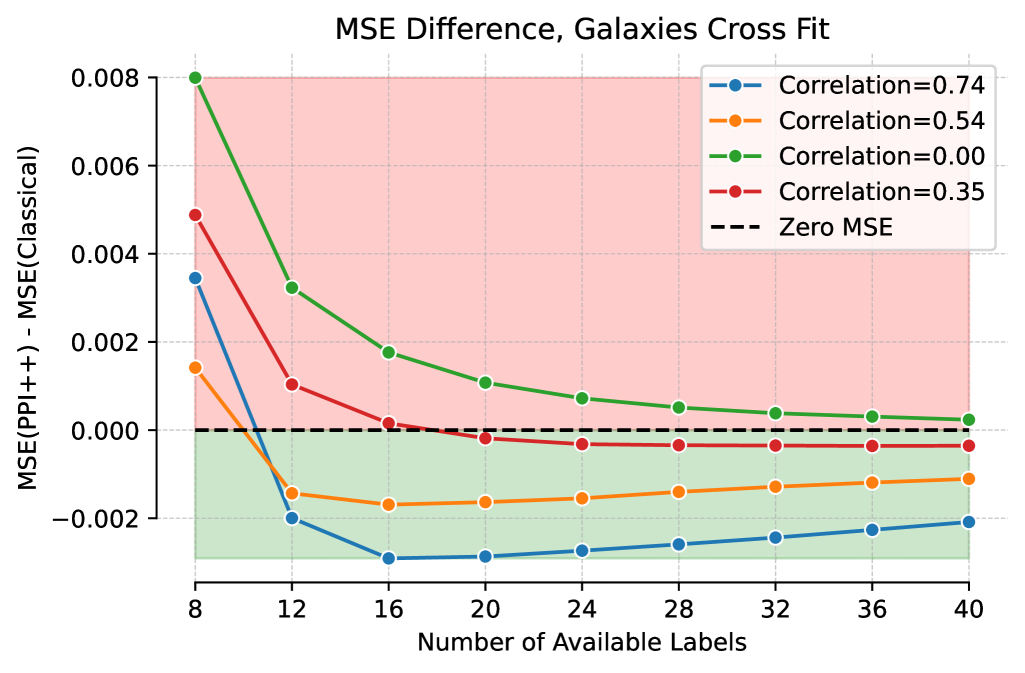
(a) Cross-fit PPI++ Estimator

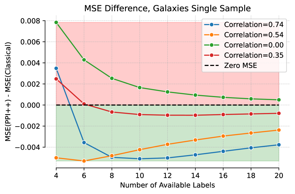
(b) Single-Sample PPI++ Estimator

Figure 3: Relative $\mathsf{MSE}$ vs. Sample Size on the Galaxies Dataset for PPI++ estimators with black-box models $f$ of varying quality. Y-axis gives the difference $\mathsf{MSE}(\hat{\theta}_{\text{PPI++}})-\mathsf{MSE}(\hat{\theta}_{\text{Classical}})$, such that lower (negative) values imply improvement over the classical estimator. Each line represents PPI++ with a different black-box model $f$. The blue line uses the original model, which has strong predictive performance, but only improves estimation error at $2n\geq 12$ (left) and $n\geq 6$ (right).

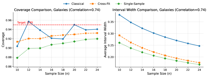
(a)

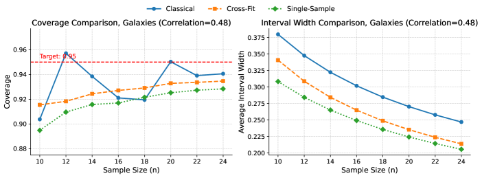
(b)

Figure 4: Comparison of Coverage and Interval Width for  (Cross-fit PPI++ Estimator, infinite $N$). and  (Single-Sample PPI++, Infinite $N$)., using different models $f$ on the Galaxies dataset. (4(a)) Original pseudo-label model $f$, where Single-Sample PPI++ has lower coverage than either Cross-fit PPI++ or the classical estimator. (4(b)) A modified model with lower correlation, where similar trends hold.

References

• Angelopoulos et al. [2023a] Anastasios N Angelopoulos, Stephen Bates, Clara Fannjiang, Michael I Jordan, and Tijana Zrnic. Prediction-powered inference. Science, 382(6671):669–674, 2023a.
• Angelopoulos et al. [2023b] Anastasios N Angelopoulos, John C Duchi, and Tijana Zrnic. Ppi++: Efficient prediction-powered inference. arXiv preprint arXiv:2311.01453, 2023b.
• Bang and Robins [2005] Heejung Bang and James M. Robins. Doubly robust estimation in missing data and causal inference models. Biometrics, 61:962–973, 12 2005. doi: 10.1111/j.1541-0420.2005.00377.x. URL https://doi.org/10.1111/j.1541-0420.2005.00377.x.
• Bates and Granger [1969] J. M. Bates and C. W. J. Granger. The combination of forecasts. Operations Research, 20:451, 12 1969. doi: 10.2307/3008764. URL https://doi.org/10.2307/3008764.
• Boyeau et al. [2024] Pierre Boyeau, Anastasios N Angelopoulos, Nir Yosef, Jitendra Malik, and Michael I Jordan. Autoeval done right: Using synthetic data for model evaluation. arXiv preprint arXiv:2403.07008, 2024.
• Broska et al. [2024] David Broska, Michael Howes, and Austin van Loon. The mixed subjects design: Treating large language models as potentially informative observations. Sociological Methods & Research, page 00491241251326865, 2024.
• Chaganty et al. [2018] Arun Tejasvi Chaganty, Stephen Mussman, and Percy Liang. The price of debiasing automatic metrics in natural language evaluation. arXiv preprint (1807.02202v1), 7 2018. URL http://arxiv.org/abs/1807.02202v1.
• Chen et al. [2021] Shuxiao Chen, Bo Zhang, and Ting Ye. Minimax rates and adaptivity in combining experimental and observational data. arXiv preprint (2109.10522), September 2021.
• Demirel et al. [2024] Ilker Demirel, Ahmed Alaa, Anthony Philippakis, and David Sontag. Prediction-powered generalization of causal inferences. arXiv preprint arXiv:2406.02873, 2024.
• Dorner et al. [2024] Florian E. Dorner, Vivian Y. Nastl, and Moritz Hardt. Limits to scalable evaluation at the frontier: Llm as judge won’t beat twice the data. arXiv preprint (2410.13341v2), 10 2024. URL http://arxiv.org/abs/2410.13341v2.
• Eyre and Madras [2024] Benjamin Eyre and David Madras. Auto-evaluation with few labels through post-hoc regression. arXiv preprint arXiv:2411.12665, 2024.
• Gligoric et al. [2025] Kristina Gligoric, Tijana Zrnic, Cinoo Lee, Emmanuel Candes, and Dan Jurafsky. Can unconfident llm annotations be used for confident conclusions? In Luis Chiruzzo, Alan Ritter, and Lu Wang, editors, Proceedings of the 2025 Conference of the Nations of the Americas Chapter of the Association for Computational Linguistics: Human Language Technologies (Volume 1: Long Papers), pages 3514–3533, Albuquerque, New Mexico, April 2025. Association for Computational Linguistics. ISBN 979-8-89176-189-6. URL https://aclanthology.org/2025.naacl-long.179/.
• Jumper et al. [2021] John Jumper, Richard Evans, Alexander Pritzel, Tim Green, Michael Figurnov, Olaf Ronneberger, Kathryn Tunyasuvunakool, Russ Bates, Augustin Žídek, Anna Potapenko, et al. Highly accurate protein structure prediction with alphafold. nature, 596(7873):583–589, 2021.
• Lavancier and Rochet [2016] F Lavancier and P Rochet. A general procedure to combine estimators. Computational statistics \& data analysis, 94:175–192, February 2016.
• Li and Ignatiadis [2025] Sida Li and Nikolaos Ignatiadis. Prediction-powered adaptive shrinkage estimation. arXiv preprint arXiv:2502.14166, 2025.
• Oberst et al. [2022] Michael Oberst, Alexander D' Amour, Minmin Chen, Yuyan Wang, David Sontag, and Steve Yadlowsky. Understanding the risks and rewards of combining unbiased and possibly biased estimators, with applications to causal inference. arXiv preprint (2205.10467v2), May 2022. URL http://arxiv.org/abs/2205.10467v2.
• Poulet et al. [2025] Pierre-Emmanuel Poulet, Maylis Tran, Sophie Tezenas du Montcel, Bruno Dubois, Stanley Durrleman, and Bruno Jedynak. Prediction-powered inference for clinical trials. medRxiv, 2025.
• Radford et al. [2021] Alec Radford, Jong Wook Kim, Chris Hallacy, Aditya Ramesh, Gabriel Goh, Sandhini Agarwal, Girish Sastry, Amanda Askell, Pamela Mishkin, Jack Clark, Gretchen Krueger, and Ilya Sutskever. Learning transferable visual models from natural language supervision. arXiv preprint (2103.00020v1), 2 2021. URL http://arxiv.org/abs/2103.00020v1.
• Yang et al. [2023] Shu Yang, Chenyin Gao, Donglin Zeng, and Xiaofei Wang. Elastic integrative analysis of randomised trial and real-world data for treatment heterogeneity estimation. Journal of the Royal Statistical Society Series B: Statistical Methodology, 85:575–596, 7 2023. doi: 10.1093/jrsssb/qkad017. URL https://doi.org/10.1093/jrsssb/qkad017.
• Zrnic and Candès [2024a] Tijana Zrnic and Emmanuel J. Candès. Active statistical inference. arXiv preprint (2403.03208v2), 3 2024a. URL http://arxiv.org/abs/2403.03208v2.
• Zrnic and Candès [2024b] Tijana Zrnic and Emmanuel J Candès. Cross-prediction-powered inference. Proceedings of the National Academy of Sciences, 121(15):e2322083121, 2024b.