Second Order Properties of Thinned Counts
in Finite Birth–Death Processes

Abstract

The paper studies the counting process arising as a subset of births and deaths in a birth–death process on a finite state space. Whenever a birth or death occurs, the process is incremented or not depending on the outcome of an independent Bernoulli experiment whose probability is a state-dependent function of the birth and death and also depends on whether it is a birth or death that has occurred. We establish a formula for the asymptotic variance rate of this process, also presented as the ratio of the asymptotic variance and the asymptotic mean. Several examples including queueing models illustrate the scope of applicability of the results. An analogous formula for the countably infinite state space is conjectured and tested.

1 Introduction

We first became aware of the second-order properties discussed in this note in various queueing models in which the simpler cases can be cast purely in a birth–death process setting where computation is more readily effected. In such cases there is a phenomenon, called BRAVO below, that appears in the limit as the state space grows. In this paper we exhibit more general processes $N_{q}$ defined by counting the births and deaths that remain after independent thinnings of these two types of events in a birth–death process and for which the BRAVO characteristics may or may not survive the thinning procedure.

Let $\{Q(t):t\geq 0\}$ be an irreducible continuous-time birth–death process on the state space ${\mathbb{J}}:=\{0,1,\ldots,J\}$ with $J<\infty$. Any realization of $Q$ is expressible in the form

$$Q(t)=Q(0)~+~N_{+}(0,t]~-~N_{-}(0,t],$$ (1.1)

where the counting measures $N_{+}$ and $N_{-}$ have unit atoms at the instants of births and deaths respectively. Thus, $N_{+}$ is the process of births in $Q$, and $N_{-}$ the process of deaths in $Q$.

We thin the sum-process $N_{+}+N_{-}$ to obtain $N_{q}$ as follows. Let $\{q^{+}_{j}:j\in\mathbb{J}\}$ and $\{q^{-}_{j}:j\in\mathbb{J}\}$ be two families of $[0,1]$-valued constants, where there is at least one $j\in{\mathbb{J}}$ where either $q_{j}^{+}>0$, or $q_{j}^{-}>0$, or both. Note that at the endpoints we set $q_{0}^{-}=0$ and $q_{J}^{+}=0$.

For each atom $s$ of $N_{+}$ let $\tilde{J}^{+}(s)=1$ with probability $q^{+}_{Q(s^{-})}$, or let $\tilde{J}^{+}(s)=0$ otherwise. Similarly, for each atom $s$ of $N_{-}$ let $\tilde{J}^{-}(s)=1$ with probability $q^{-}_{Q(s^{-})}\,$, or let $\tilde{J}^{-}(s)=0$ otherwise. Hence the probability of having atoms for $\tilde{J}^{+}$ and $\tilde{J}^{-}$ depend on the state of $Q$ just before the jump. Now let

$$N_{q}(0,t]=\int_{0}^{t}\tilde{J}^{+}(u)\,N_{+}({\rm d}u)~+~\int_{0}^{t}\tilde{J}^{-}(u)\,N_{-}({\rm d}u),$$ (1.2)

where conditional on $\{Q(u):u<t^{\prime}\}$ for any finite $t^{\prime}$, all indicator r.v.s $\tilde{J}^{\pm}(t)$ for $t<t^{\prime}$ are mutually independent.

This paper studies the asymptotic variance also represented via the asymptotic index of dispersion of $N_{q}$,

$$\mathcal{D}:=\lim_{t\to\infty}\frac{\mathop{\rm var}\nolimits N_{q}(0,t]}{{\mathbb{E}}\big{[}N_{q}(0,t]\big{]}}.$$ (1.3)

In mathematical biology, for a general stationary counting process $N_{q}$, $\mathcal{D}$ is known as the Fano factor, as for example in Eden and Kramer [6]. The denominator and numerator here are asymptotically linear in $t\geq 0$, and the limit in (1.3) is always finite and positive. Our main result, Theorem 1, presents a formula for $\mathcal{D}$ in terms of $\{q^{\pm}_{j}:j\in\mathbb{J}\}$ and the birth- and death-rates of $Q$. To our knowledge this condensed explicit formula is new. Yet we mention that since the state space is finite, computable matrix based expressions for $\mathcal{D}$ can be obtained by considering the process as a MAP (Markovian Arrival Process); see for example [9].

In the special case of a pure death-counting process (all $q_{i}^{+}=0$), no thinning ($q^{-}_{i}\equiv 1$), a similar formula was derived in [14] where the BRAVO effect was first noted. This phenomenon occurs when the birth–death process $Q(t)$ models a queueing system and $N_{-}$ is the output process of served customers. In a sequence of papers associated with BRAVO [4, 5, 7, 8, 11, 12, 13, 14], it was shown that for non-small $J$, it holds that $\mathcal{D}\approx 1$, except for ‘balanced‘ singular cases in which the arrival rate equals the service capacity. In those cases $\mathcal{D}\approx{\cal B}$ where for many standard queueing models, the BRAVO constant ${\cal B}<1$. This constant equals $2/3$ for simple single-server Markovian queues with a finite buffer, [8, 14]; equals $2(1-2/\pi)\approx 0.7268$ for infinite buffer cases with infinite buffers, [1, 13]; and equals $\approx 0.6093$ in many-server queues under the so-called Halfin–Whitt scaling regime, [5]. Note also a correction paper for some of the computations associated with that result, [11].

Further, for queues with renewal input (i.e. GI/$\cdot/\cdot)$ systems), the first multiple, $2$, in $2(1-2/\pi)$ is replaced by the sum of the squared coefficients of variation of the inter-arrival and service times driving a GI/G/$s$ queue, [1]; similarly in the finite case, as conjectured and numerically tested, [12], ${\cal B}$ equals the sum of the squared coefficients of variations divided by $3$. All of these examples motivate the study of the asymptotic index of dispersion, $\mathcal{D}$.

For simple queueing models with reneging, the question of the existence of BRAVO remains. When such queueing processes are represented by birth–death models, a thinning mechanism is required, since some deaths count as departures but others are reneging customers. This motivated us to seek a general formula for $\mathcal{D}$. Here we prove our formula for $\mathcal{D}$ for the finite ${\mathbb{J}}$ case. We also explore its use for the countably infinite case, and leave the exact conditions of when this infinite case holds for further research. Our derivation follows from detailed regenerative arguments, including the manipulation of moment expressions via matrix algebra. The derivation also hinges on an explicit inverse of a matrix, which to the best of our knowledge has not appeared earlier in this form, and can in principle be used for other birth and death related results.

The paper is organized as follows. In Section 2 we present the main result, Theorem 1. We then prove the main result in Section 3. The proof hinges on an explicit formula for the inverse of a matrix which may be of independent interest and is also presented as a lemma in Section 3. We close with examples in Section 4.

2 Setup and Main Result

Let $\{Q(t),t\geq 0\}$ be an irreducible continuous-time birth–death (BD) Markov chain on finite state space $\mathbb{J}:=\{0,1,\ldots,J\}$, for finite positive integer $J$. The birth rates are $\lambda_{0},\ldots,\lambda_{J}$ and death rates are $\mu_{0},\ldots,\mu_{J}$ with $\lambda_{J}=\mu_{0}=0$ and all other rates positive.

The stationary (and limiting) probabilities $\pi_{i}:=\lim_{t\to\infty}\mathbb{P}\{Q(t)=i\}$ satisfy the partial balance relations

$$\pi_{i}\mu_{i}=\pi_{i-1}\lambda_{i-1}\qquad\text{for}\qquad i\in\mathbb{J}\setminus\{0\},$$ (2.1)

and therefore

$$\pi_{i}=\frac{\prod_{k=1}^{i}(\lambda_{k-1}/\mu_{k})}{\sum_{j\in\mathbb{J}}\prod_{k=1}^{j}(\lambda_{k-1}/\mu_{k})}\,=\,\pi_{0}\prod_{k=1}^{i}\frac{\lambda_{k-1}}{\mu_{k}}\qquad\text{for}\qquad i\in\mathbb{J},$$ (2.2)

with empty products being unity (so $\pi_{0}\neq 0$). We denote the cumulative distribution elements as

$$P_{k}:=\sum_{i=0}^{k}\pi_{i},\qquad\text{for}\qquad k\in\mathbb{J}.$$ (2.3)

Denote the raw rate of births deaths as,

$${\overline{\lambda}}_{\star}=\sum_{i\in\mathbb{J}}\pi_{i}(\lambda_{i}+\mu_{i})=2\sum_{i\in\mathbb{J}}\pi_{i}\lambda_{i},$$ (2.4)

where the second equality follows from (2.1). The rate ${\overline{\lambda}}_{\star}$ satisfies,

$$\lim_{t\to\infty}\frac{{\mathbb{E}}\big{[}N_{+}(0,t]+N_{-}(0,t]\big{]}}{t}={\overline{\lambda}}_{\star}.$$

With each state $i\in\mathbb{J}$, associate the probabilities $q^{\pm}_{i}\in[0,1]$ and let $N_{q}(\cdot)$ denote the thinned sum-process based on $Q$ as described in (1.2). With this, define the thinned rate as

$${\overline{\lambda}}=\sum_{i\in\mathbb{J}}\pi_{i}(\lambda_{i}q^{+}_{i}+\mu_{i}q^{-}_{i}).$$ (2.5)

This rate ${\overline{\lambda}}$ satisfies,

$$\lim_{t\to\infty}\frac{{\mathbb{E}}\big{[}N_{q}(0,t]\big{]}}{t}={\overline{\lambda}}.$$

Note also that ergodicity shows that in the long run $N_{q}(\cdot)$ counts a proportion $\varpi$ of all births and deaths, where

$$\varpi=\frac{{\overline{\lambda}}}{{\overline{\lambda}}_{\star}}=\lim_{t\to\infty}\frac{{\mathbb{E}}\big{[}N_{q}(0,t]\big{]}}{{\mathbb{E}}\big{[}N_{+}(0,t]+N_{-}(0,t]\big{]}}=\lim_{t\to\infty}{\mathbb{E}}\Big{[}\frac{N_{q}(0,t]}{N_{+}(0,t]+N_{-}(0,t]}\Big{]}.$$ (2.6)

Also note that,

$${\overline{\lambda}}=\sum_{i=0}^{J-1}\pi_{i}\lambda_{i}q^{+}_{i}+\sum_{i=1}^{J}\pi_{i}\mu_{i}q^{-}_{i}=\sum_{i=0}^{J-1}\pi_{i}\lambda_{i}(q^{+}_{i}+q^{-}_{i+1}),$$ (2.7)

where the last equality follows using (2.1).

We also use the partial sums

$${\overline{\lambda}}_{k}:=\sum_{i=0}^{k}\pi_{i}\lambda_{i}q^{+}_{i}+\sum_{i=1}^{k}\pi_{i}\mu_{i}q^{-}_{i}=\pi_{k}\lambda_{k}q_{k}^{+}+\sum_{i=0}^{k-1}\pi_{i}\lambda_{i}(q^{+}_{i}+q^{-}_{i+1}),$$ (2.8)

and observe that ${\overline{\lambda}}_{J}={\overline{\lambda}}$. Further, when normalized as

$$\Lambda_{k}:=\frac{{\overline{\lambda}}_{k}}{{\overline{\lambda}}}\,=\,\frac{\pi_{k}\lambda_{k}q^{+}_{k}+\sum_{i=0}^{k-1}\pi_{i}\lambda_{i}(q^{+}_{i}+q_{i+1}^{-})}{{\overline{\lambda}}}\qquad\text{for}\qquad k\in\mathbb{J},$$ (2.9)

$\{\Lambda_{k}\}$ defines a cumulative distribution in the same manner that $\{P_{k}\}$ does.

Theorem 1 presents a formula for the asymptotic index of dispersion $\mathcal{D}$ at (1.3) in terms of the distribution functions $\{P_{k}\}$ and $\{\Lambda_{k}\}$, the counting rate ${\overline{\lambda}}$ and the sequences $\{q_{k}^{\pm}\}$, $\{\lambda_{k}\}$ and $\{\pi_{k}\}$. If $N_{q}(\cdot)$ were a Poisson process we should have $\mathcal{D}=1$. This is certainly not the case in general. Our formula directly generalizes Theorem 1 of [14] which handles the pure death-counting process case of $q_{i}^{-}\equiv 1$ and $q_{i}^{+}\equiv 0$; so $N_{q}(0,t]=N_{-}(0,t]$ as in (1.1). The result in [14] is proved by combining results for Markovian Arrival Processes with limit results for Markov Modulated Poisson Processes; the method there requires the retention probabilities $q_{i}^{\pm}$ to be $\{0,1\}$-valued. Our proof is quite different: it is more elementary, albeit with tedious calculations; importantly, it no longer requires $q_{i}^{-}=1$ and $q_{i}^{+}=0$.

Theorem 1.

Consider the finite state space case where irreducible $Q(\cdot)$ follows any initial distribution on $\mathbb{J}$. The asymptotic index of dispersion of $N_{q}$ is,

$$\mathcal{D}=1+2\sum_{k=0}^{J-1}R_{k},$$ (2.10)

where,

$$R_{k}=(P_{k}-\Lambda_{k})\bigg{(}\frac{{\overline{\lambda}}(P_{k}-\Lambda_{k})}{\pi_{k}\lambda_{k}}+q^{+}_{k}-q^{-}_{k+1}\bigg{)}.$$ (2.11)

The Infinite State Space Case

While Theorem 1 is limited to a finite state space, a natural extension is to consider a countably infinite state space where $\lambda_{i}>0$ for all all $i\geq 0$, $\mu_{i}>0$ for all $i\geq 1$, and $q^{\pm}_{i}$ are defined for all $i\geq 0$ with $q_{0}^{-}=0$. In such a case, we also require the standard stability (positive recurrance) condition,

$$\sum_{j\in\mathbb{J}}\prod_{k=1}^{j}\frac{\lambda_{k-1}}{\mu_{k}}<\infty.$$ (2.12)

In this infinite state space case, $P_{k}$, $\lambda_{k}$, $\Lambda_{k}$, and ${\overline{\lambda}}$ extend naturally as above with,

$${\overline{\lambda}}=\sum_{i=0}^{\infty}\pi_{i}\lambda_{i}(q^{+}_{i}+q^{-}_{i+1}).$$ (2.13)

Now using $R_{k}$ as in (2.11) we define the formal expression,

$$\mathcal{D}_{\infty}=1+2\sum_{k=0}^{\infty}R_{k}.$$ (2.14)

While in this paper we do not prove that $\mathcal{D}_{\infty}$ equals the asymptotic index of dispersion $\mathcal{D}$ of (1.3), we conjecture that under suitable regularity conditions, the expression for $\mathcal{D}_{\infty}$ evaluates to the asymptotic index of dispersion in the countably infinite state space case. Some insightful examples and numerical results involving the expression (2.14) are presented in Section 4.

Special Cases

We say the process is a pure birth-counting process if $q_{i}^{-}=0$ for all states $i$ and $q_{i}^{+}>0$ for at least one state $i$ (note that this term should not be confused with a pure-birth process which is a process with $\mu_{i}=0$ for all $i$). Similarly a pure death-counting process has $q_{i}^{+}=0$ for all state $i$ and $q_{i}^{-}>0$ for at least one state $i$. Further, we call $N(0,t]$ a fully counting pure-birth process if in addition to being pure birth-counting it also has $q_{i}^{+}=1$ for all states $i$. And similarly a fully counting pure-death process is a pure death-counting process that has $q_{i}^{-}=1$ for all states $i$. Finally we call the process fully counting if $q_{i}^{+}=1$ and $q_{i}^{-}=1$ for all states $i$.

Let us see that our finite state space formula, (2.10) from Theorem 1 generalizes the formula, in Theorem 3.1 of [14]. Specifically, [14] studies fully counting pure-death processes, and by switching the role of births and deaths, one may also apply the results to fully counting pure-birth processes. The following corollary applies to this case and one may verify that (2.15) agrees with the results in Theorem 3.1 of [14].

Corollary 1.

Given a fixed set of birth and death parameters, $\mathcal{D}$ is the same for both the fully counting pure-birth process case, or the fully counting pure-death case. In both of these cases,

$$\mathcal{D}=1+2{\overline{\lambda}}\sum_{k=0}^{J-1}\frac{\bigg{(}P_{k}-\Lambda_{k}^{-}\bigg{)}\bigg{(}P_{k}-\Lambda_{k}^{+}\bigg{)}}{\pi_{k}\lambda_{k}},$$ (2.15)

where

$$\Lambda_{k}^{-}=\frac{\sum_{i=0}^{k-1}\pi_{i}\lambda_{i}}{{\overline{\lambda}}},\qquad\text{and}\qquad\Lambda_{k}^{+}=\frac{\sum_{i=0}^{k}\pi_{i}\lambda_{i}}{{\overline{\lambda}}}.$$ (2.16)

Note that in the fully counting pure-birth case, $\Lambda_{k}$ of (2.9) is $\Lambda_{k}^{+}$ of (2.16) and similarly in the fully counting pure-death case, $\Lambda_{k}$ is $\Lambda_{k}^{-}$. Note also that we take $\Lambda_{0}^{-}=0$.

Proof.

It follows from Equation (2.5) and (2.1) that ${\overline{\lambda}}=\sum_{j=0}^{J-1}\pi_{j}\lambda_{j}$ for both the fully counting pure-birth and fully counting pure-death process. However, considering (2.9) we see that $\Lambda_{k}$ differs for these cases and is $\Lambda_{k}^{-}$ and $\Lambda_{k}^{+}$ for the fully counting pure-death and fully counting pure-birth processes respectively.

Now using Theorem 1, for the fully counting pure-birth case we obtain the following expression for $R_{k}$ in (2.11),

$$R_{k} =(P_{k}-\Lambda_{k})\bigg{(}\frac{{\overline{\lambda}}(P_{k}-\Lambda_{k})}{\pi_{k}\lambda_{k}}+1\bigg{)}$$

$$=(P_{k}-\Lambda_{k})\bigg{(}\frac{{\overline{\lambda}}(P_{k}-\Lambda_{k-1})}{\pi_{k}\lambda_{k}}\bigg{)}$$

$$={\overline{\lambda}}\frac{\bigg{(}P_{k}-\Lambda_{k}^{-}\bigg{)}\bigg{(}P_{k}-\Lambda_{k}^{+}\bigg{)}}{\pi_{k}\lambda_{k}}.$$

Similarly, for the fully counting pure-death we obtain the same expression on the right hand side. Hence we obtain (2.15) for both of these cases.

∎

3 Proof of the main result

We break up the proof into several subsections. First we present a lemma for an explicit inverse of a $J\times J$ matrix. This result maybe of independent interest. Then we construct a renewal-reward process related to $N_{q}$. Then we compute the asymptotic variance of the renewal reward process based on moments of quantities within a regeneration period. We then carry out a Laplace transform with generating function analysis, to obtain expressions for these moments. Finally, we use the explicit matrix inverse to assemble the pieces together and obtain the result.

An Explicit Matrix Inverse

Define the following $J\times J$ matrix,

$${\mathbf{W}}=\left[\begin{array}[]{cccccccc}r_{1}&-\lambda_{1}&0&.&\cdots&.&0\\ -\mu_{2}&r_{2}&-\lambda_{2}&0&\cdots&.&.\\ 0&-\mu_{3}&r_{3}&-\lambda_{3}&\cdots&.&.\\ .&0&\ddots&\ddots&\ddots&\vdots&\vdots\\ \vdots&\vdots&\ddots&\ddots&\ddots&\ddots&0\\ .&.&.&\cdot&-\mu_{J-1}&r_{J-1}&-\lambda_{J-1}\\ 0&.&.&\cdots&0&-\mu_{J}&r_{J}\\ \end{array}\right],$$ (3.1)

where $r_{i}=\lambda_{i}+\mu_{i}$, and $\lambda_{i},\mu_{i}>0$.

Based on computational exploration with trial and error, we were able to guess an explicit form for the matrix inverse.

Lemma 1.

The matrix ${\mathbf{W}}$ is non-singular with elements of the inverse given by,

$$\big{(}{\mathbf{W}}^{-1}\big{)}_{ij}=\sum_{k=1}^{\min\{i,j\}}\frac{\pi_{j}}{\pi_{k}\mu_{k}}\qquad(i,j=1,\ldots,J).$$ (3.2)

Proof.

Write ${\mathbf{W}}=(w_{ij}),\ {\mathbf{W}}^{-1}=(u_{ij})$. We leave the reader to check the case $i=j=J$, namely $({\mathbf{W}}^{-1}{\mathbf{W}})_{JJ}=1$. Otherwise,

$$({\mathbf{W}}^{-1}{\mathbf{W}})_{11}=u_{11}w_{11}+u_{12}w_{21}=\frac{\pi_{1}}{\pi_{1}\mu_{1}}(\lambda_{1}+\mu_{1})-\frac{\pi_{2}}{\pi_{1}\mu_{1}}\mu_{2}=1;$$

for $i=1$ and $j=2,\ldots,J,$

$$({\mathbf{W}}^{-1}{\mathbf{W}})_{1j} =u_{1,j-1}w_{j-1,j}+u_{1j}w_{jj}+u_{1,j+1}w_{j+1,j}$$

$$=\frac{\pi_{j-1}}{\pi_{1}\mu_{1}}\bigg{[}-\lambda_{j-1}+\frac{\lambda_{j-1}}{\mu_{j}}(\lambda_{j}+\mu_{j})-\frac{\lambda_{j-1}\lambda_{j}}{\mu_{j}\mu_{j+1}}\mu_{j+1}\bigg{]}=0;$$

for $i,j\geq 2,\;i\neq j$,

$$({\mathbf{W}}^{-1}{\mathbf{W}})_{ij} =u_{i,j-1}w_{j-1,j}+u_{ij}w_{jj}+u_{i,j+1}w_{j+1,j}$$

$$=-u_{i,j-1}\lambda_{j-1}+u_{ij}(\lambda_{j}+\mu_{j})-u_{i,j+1}\mu_{j+1}$$

$$=\bigg{(}\sum_{k=1}^{\min\{i,j\}}\frac{1}{\pi_{k}\mu_{k}}\bigg{)}\pi_{j-1}\bigg{[}-\lambda_{j-1}+\frac{\pi_{j}}{\pi_{j-1}}(\lambda_{j}+\mu_{j})-\frac{\pi_{j+1}}{\pi_{j-1}}\mu_{j+1}\bigg{]}=0;$$

and for $2\leq i=j\leq J-1$,

$$({\mathbf{W}}^{-1}{\mathbf{W}})_{ii} =u_{i,i-1}w_{i-1,i}+u_{ii}w_{ii}+u_{i,i+1}w_{i+1,i}$$

$$=-u_{i,i-1}\lambda_{i-1}+u_{ii}(\lambda_{i}+\mu_{i})-u_{i,i+1}\mu_{i+1}$$

$$=\bigg{(}\sum_{k=1}^{i-1}\frac{1}{\pi_{k}\mu_{k}}\bigg{)}\pi_{i-1}\bigg{[}-\lambda_{i-1}+\frac{\pi_{i}}{\pi_{i-1}}(\lambda_{i}+\mu_{i})-\frac{\pi_{i+1}}{\pi_{i-1}}\mu_{i+1}\bigg{]}$$

$$\qquad\qquad\qquad+\frac{\pi_{i}}{\pi_{i}\mu_{i}}\Big{[}(\lambda_{i}+\mu_{i})-\frac{\pi_{i+1}}{\pi_{i}}\mu_{i+1}\Big{]}\,=\,0+1\,=\,1.$$

Combining these cases confirms (3.2). ∎

A Renewal Reward Process

We exploit regeneration epochs in the sample path of the BD process $Q$ at exit times $\tilde{t}$ from the state 0, i.e. $\{Q(\tilde{t}-)=0,Q(\tilde{t})=1\}$, focusing on the generic time $X$ that elapses between such epochs and the number $Y$ of birth and death epochs that are counted (i.e. are not thinned) by the counting function $N(\cdot)$ during this time-interval of length $X$. Then $N(\cdot)$ has asymptotic behaviour the same as a renewal–reward process $C(\cdot)$ for which $\lim_{t\to\infty}t^{-1}\mathop{\rm var}\nolimits C(t)$ is known ([3] and (3.9)–(3.11) below). This derivation shows that the initial distribution of $Q(0)$ plays no part in the theorem when $J$ is finite, i.e. the result depends only on the existence and properties of a stationary distribution $\{\pi_{i}\}$, and thus holds both for a stationary and non-stationary version of the process.

Let ${\cal T}$ be the set of regeneration times in $\mathbb{R}_{+}$ when $Q(\cdot)$ exits the state 0, i.e.

$${\cal T}=\{\tilde{t}:Q(\tilde{t}-)=0,\,Q(\tilde{t})=1\}.$$ (3.3)

Because $\pi_{0}>0$, ${\cal T}$ is a countably infinite sequence which a.s. has no finite limit point; enumerate ${\cal T}$ as the increasing sequence $\{T_{i}\}$. Denote

$$X_{i}=T_{i}-T_{i-1}\quad(i=1,2,\ldots),$$ (3.4)

and write $Y_{i}=N_{q}(T_{i-1},T_{i}]$ for the number of transitions counted (after thinning) during the half-open time interval shown. Write also

$$\tilde{n}^{\pm}_{i,j}:=\mathop{\rm{card}}\nolimits\big{\{}t\in(T_{i-1},T_{i}]:Q(t-)=j,\ Q(t)=j\pm 1\big{\}},$$ (3.5)

respectively, for which almost surely for every $i$, $\tilde{n}^{-}_{i,0}=0$, $\tilde{n}^{+}_{i,0}=1=\tilde{n}^{-}_{i,1}$, $\tilde{n}^{+}_{i,j}=\tilde{n}^{-}_{i,j+1}\in\{0,1,\ldots\}$ for $j=1,\ldots,J-1$, and

$$Y_{i}:=\sum\nolimits_{j=0}^{J-1}\mbox{Bin}(\tilde{n}^{+}_{i,j},\,q^{+}_{j})+\sum\nolimits_{j=1}^{J}\mbox{Bin}(\tilde{n}^{-}_{i,j},\,q^{-}_{j})=:Y_{i}^{+}+Y_{i}^{-}\,,$$ (3.6)

say, where $\mathop{\rm{Bin}}\nolimits(k,p)$ denotes a binomial $(k,p)$ r.v. Because the process $Q(\cdot)$ has the strong Markov property, the sequence $\big{\{}(X_{i},Y_{i}),i\geq 1\big{\}}$ is a sequence of i.i.d. random vectors. Let $(X,Y)$ denote a generic element of this sequence. Define

$$N_{\cal T}(t):=\sup\Big{\{}\ell:\sum\nolimits_{i=1}^{\ell}X_{i}\leq t\Big{\}},\qquad C(t)=\sum\nolimits_{i=1}^{N_{\cal T}(t)}Y_{i}.$$ (3.7)

Then $C(\cdot)$ is a renewal–reward process; $C(t)$ is the number of BD transitions counted during regeneration intervals $X_{i}$ wholly contained in $(0,t]$, and (3.7) exhibits $Y_{i}$ as the sum of counted BD transitions accumulating during each interval $X_{i}$ and finally included in $C(\cdot)$ at the regeneration epochs occurring by $t$. From our definitions,

$$N_{q}(0,t]=C(t)+\widetilde{N}_{q}(t),$$ (3.8)

where $\widetilde{N}_{q}(t)$ is the number of counted BD transitions occurring in the time interval $(T_{N_{q}(t)-1},t]$. Take first and second moments of both sides of (3.8), divide by $t$ and let $t\to\infty$. Then

$$\lim_{t\to\infty}\frac{{\mathbb{E}}\big{[}N_{q}(0,t]\big{]}}{t} =\lim_{t\to\infty}\frac{{\mathbb{E}}\big{[}C(t)\big{]}}{t},$$ (3.9)

$$\lim_{t\to\infty}\frac{\mathop{\rm var}\nolimits N_{q}(0,t]}{t} =\lim_{t\to\infty}\frac{\mathop{\rm var}\nolimits C(t)}{t},$$

where we have used the fact that ${\mathbb{E}}\big{[}\big{(}\widetilde{N_{q}}(t)\big{)}^{2}\big{]}<\infty$, hence $\mathop{\rm cov}\nolimits\big{(}C(t),\widetilde{N}_{q}(t)\big{)}=O(\sqrt{t}\,)$. The two limit relations at (3.9) imply that

$$\mathcal{D}=\lim_{t\to\infty}\frac{\mathop{\rm var}\nolimits C(t)}{{\mathbb{E}}\big{[}C(t)\big{]}},$$ (3.10)

and thus we may study $C(t)$ in place of $N_{q}(0,t]$.

A representation of the asymptotic variance of renewal–reward processes in terms of moments of a generic element $(X,Y)$ is long known (see [3]), from which work it follows that when $X$ and $Y$ have finite second-order moments,

$$\mathcal{D}=\frac{\mathop{\rm var}\nolimits\big{(}Y-{\mathbb{E}}[Y](X/{\mathbb{E}}[X])\big{)}}{{\mathbb{E}}[Y]}=\frac{{\mathbb{E}}(Y^{2})-2R\,{\mathbb{E}}(XY)+R^{2}\,{\mathbb{E}}(X^{2})}{{\mathbb{E}}(Y)},$$ (3.11)

where $R={\mathbb{E}}(Y)/{\mathbb{E}}(X)$, showing that $\mathcal{D}$ is determined by ${\mathbb{E}}[X]$, ${\mathbb{E}}[Y]$, ${\mathbb{E}}[XY]$, ${\mathbb{E}}[X^{2}]$ and ${\mathbb{E}}[Y^{2}]$. In (3.11), $Y$ is the number of counted births and deaths in a generic regeneration interval of duration $X$, being a generic recurrence time of the state 0 of the stationary Markov process $Q$, so ${\mathbb{E}}(X)=1/(\pi_{0}\lambda_{0})$. Births and deaths occur in $Q$ at rate ${\overline{\lambda}}_{\star}$, and $N_{q}(\cdot)$ counts a proportion $\varpi$ of these (see (2.6)) at rate ${\overline{\lambda}}=\varpi{\overline{\lambda}}_{\star}$, so for the pair $(X,Y)$, the mean count ${\mathbb{E}}(Y)$ equals $\varpi{\overline{\lambda}}_{\star}{\mathbb{E}}(X)$. Thus, $R={\mathbb{E}}(Y)/{\mathbb{E}}(X)={\overline{\lambda}}$ and ${\mathbb{E}}(Y)={\overline{\lambda}}/(\pi_{0}\lambda_{0})$.

To compute these moments we study the evolution of the $\mathbb{J}$-valued strong Markov process $Q$ in more detail over a generic regeneration interval. Consider the r.v.s, for $j,k=1,\ldots,J$,

$$\tau_{k} :=\inf\{t>0:Q(t)=0\mid Q(0)=k\},$$

$$\breve{n}^{\pm}_{j,k} :=\mathop{\rm{card}}\nolimits\big{\{}t\in(0,\tau_{k}]:Q(t-)=j,\,Q(t)=j\pm 1\mid Q(0)=k\big{\}},$$ (3.12)

$$N_{J}(\tau_{k}) :=\big{(}\textstyle\sum_{j=1}^{J-1}\mathop{\rm{Bin}}\nolimits(\breve{n}^{+}_{j,k},q^{+}_{j})+\sum_{j=1}^{J}\mathop{\rm{Bin}}\nolimits(\breve{n}^{-}_{j,k},q^{-}_{j})\mid Q(0)=k\big{)},$$

where for given $k$ and $\breve{n}^{\pm}_{j,k}$, each of the sequences of binomial r.v.s $\{\mathop{\rm{Bin}}\nolimits(\breve{n}^{\pm}_{j,k},q^{\pm}_{j}):j=1,\ldots,J\}$ has mutually independent elements. (Strictly, each of the r.v.s defined in (3) is a functional defined on the sample path $\{Q(u):0\leq u\leq\tau_{k}\}$, where given the sample path, each of $\breve{n}^{\pm}_{j,k}$ records the numbers of births or deaths resp., and then, conditional on these numbers, $N_{J}(\tau_{k})$ counts the number of births or deaths included in the two components of $N_{q}(\cdot)$ at (1.2) over the regenerative interval $X_{i}$ of which $\tau_{k}$ is part; so, conditional on the sample path of $Q(\cdot)$, hence also $\{\breve{n}^{\pm}_{j,k}\}$, $N_{J}$ has the representation as shown in terms of independent Binomial r.v.s.). Note the distinction between the counting r.v.s $\breve{n}^{\pm}_{j,k}$ here and $\tilde{n}^{\pm}_{i,j}$ in (3.5).

Any regeneration interval $X_{i}$ as at (3.4) starting at time $T_{i-1}$ consists first of an interval which we call the busy period, and then of an interval which we call the idle period. The busy period is distributed as $\tau_{1}$ and the idle period is distributed as an exponential random variable, say $\sigma_{0}$, with rate $\lambda_{0}$. With this, $X_{i}=^{d}\tau_{1}+\sigma_{0}$, and $Y_{i}=^{d}N_{J}(\tau_{1})+\mathop{\rm{Bin}}\nolimits(1,q_{0}^{+})$. In these representations, $\sigma_{0}$ is independent of both $\tau_{1}$ and $N_{J}(\tau_{1})$, and $\mathop{\rm{Bin}}\nolimits(1,q_{0}^{+})$ and $N_{J}(\tau_{1})$ are independent; of course $\tau_{1}$ and $N_{J}(\tau_{1})$ are in general dependent.

For $h=1,2$, define the moments

$$\tau^{(h)}_{k} ={\mathbb{E}}[\tau_{k}^{h}]\,=\,{\mathbb{E}}[\tau_{k}^{h}\mid Q(0)=k],$$

$$n^{(h)}_{k} ={\mathbb{E}}\big{[}\big{(}N_{J}(\tau_{k})\big{)}^{h}\mid Q(0)=k\big{]},$$ (3.13)

$$c_{k}^{(1)} ={\mathbb{E}}[\tau_{k}\,N_{J}(\tau_{k})\mid Q(0)=k].$$

Observe that $\tau^{(1)}_{0}=n^{(1)}_{0}=c^{(1)}_{0}=\tau^{(2)}_{0}=n^{(2)}_{0}=0$. Below we develop expressions for the moments $\tau_{1}^{(1)}$, $n^{(1)}_{1}$, $c^{(1)}_{1}$, $\tau^{(2)}_{1}$ and $n^{(2)}_{1}$, using these to find the moments ${\mathbb{E}}[XY]$, ${\mathbb{E}}[X^{2}]$, and ${\mathbb{E}}[Y^{2}]$ for (3.11). Recalling the expressions for ${\mathbb{E}}[X]$, ${\mathbb{E}}[Y]$ we have

$${\mathbb{E}}[X] =\tau_{1}^{(1)}+\frac{1}{\lambda_{0}}=\frac{1}{\pi_{0}\lambda_{0}},$$ (3.14)

$${\mathbb{E}}[Y] =n_{1}^{(1)}+q_{0}^{+}\,=\,\frac{{\overline{\lambda}}}{\pi_{0}\lambda_{0}}.$$

And thus,

$$\tau_{1}^{(1)}=(1-\pi_{0})/(\pi_{0}\lambda_{0}),\qquad\text{and}\qquad n_{1}^{(1)}=({\overline{\lambda}}-\pi_{0}\lambda_{0}q_{0}^{+})/(\pi_{0}\lambda_{0}).$$ (3.15)

Now continuing with the busy period and idle period relationship we have,

$${\mathbb{E}}[X^{2}] =\tau_{1}^{(2)}+\frac{2\tau_{1}^{(1)}}{\lambda_{0}}+\frac{2}{\lambda_{0}^{2}}\,=\,\tau_{1}^{(2)}+\frac{2}{\pi_{0}\lambda_{0}^{2}}\,,$$ (3.16)

$${\mathbb{E}}[XY] =c_{1}^{(1)}+\frac{n_{1}^{(1)}}{\lambda_{0}}+q_{0}^{+}\Big{(}\tau_{1}^{(1)}+\frac{1}{\lambda_{0}}\Big{)}\,=\,c_{1}^{(1)}+\frac{n_{1}^{(1)}}{\lambda_{0}}+\frac{q_{0}^{+}}{\pi_{0}\lambda_{0}}\,,$$

$${\mathbb{E}}[Y^{2}] =n_{1}^{(2)}+2n_{1}^{(1)}q_{0}^{+}+q_{0}^{+}\,.$$

Now using (3.11) and (3.15) we have,

$${\mathbb{E}}(Y)\mathcal{D}=n_{1}^{(2)}-2{\overline{\lambda}}c_{1}^{(1)}+{\overline{\lambda}}^{2}\tau_{1}^{(2)}+q_{0}^{+}\Big{(}1-2q_{0}^{+}+2\pi_{0}{\mathbb{E}}(Y)\Big{)}.$$ (3.17)

A Transform Based Calculation

To use (3.17), we now find a representation for the moments $n_{1}^{(2)}$, $c_{1}^{(1)}$, and $\tau_{1}^{(2)}$ using first step analysis. Note that this process also yields expressions for the first moments $\tau_{1}^{(1)}$ and $n_{1}^{(1)}$ which naturally agree with those computed above. For such a first step analysis, the r.v.s at (3) are amenable to study via a backwards decomposition in terms of the BD process $Q$ as follows. Given $Q(0)=k$ for some $k=1,\ldots,J$, define $\phi_{k}(s,z)={\mathbb{E}}[{\rm e}^{-s\tau_{k}}z^{N_{J}(\tau_{k})}\mid Q(0)=k]$. The first transition in $Q$ from $Q(0)=k$ occurs after the random time $\sigma_{k}$ which is exponentially distributed with mean $1/r_{k}:=1/(\lambda_{k}+\mu_{k})$, after which $Q=k\pm 1$ (at rate $\lambda_{k}$ for +1, and $\mu_{k}$ for $-1$), and $N_{J}(\tau_{k})$ increases by 1 with probability $q_{k}^{\pm}$ depending on $\pm 1$ change in $Q$. Using indicator r.v.s $I(q)=1$ with probability $q$, $=0$ otherwise, these relations can be written as

$$(\tau_{k},N_{J}(\tau_{k}))=\Bigg{\{}\begin{aligned} &\big{(}\sigma_{k}+\tau_{k+1},\,I(q_{k}^{+})+N_{J}(\tau_{k+1})\big{)}\;\;\text{with prob. }\lambda_{k}/r_{k},\\ &\big{(}\sigma_{k}+\tau_{k-1},\,I(q_{k}^{-})+N_{J}(\tau_{k-1})\big{)}\;\;\text{with prob. }\mu_{k}/r_{k}.\\ \end{aligned}$$ (3.18)

Using generating functions and ${\mathbb{E}}[{\rm e}^{-s\sigma_{k}}]=r_{k}/(s+r_{k})$ we deduce that

$$(s+r_{k})\phi_{k}(s,z)=\lambda_{k}(zq_{k}^{+}+1-q_{k}^{+})\phi_{k+1}(s,z)+\mu_{k}(zq_{k}^{-}+1-q_{k}^{-})\phi_{k-1}(s,z).$$ (3.19)

Differentiation in $s$ and $z$ and setting $(s,z)=(0,1)$ yields the relations for $k=1,\ldots,J$ (we can and do include $k=1$ and $k=J$ because $\lambda_{J}=0$ and $\tau^{(1)}_{0}=n^{(1)}_{0}=c^{(1)}_{0}=\tau^{(2)}_{0}=n^{(2)}_{0}=0$):

$$r_{k}\tau^{(1)}_{k}-\lambda_{k}\tau^{(1)}_{k+1}-\mu_{k}\tau^{(1)}_{k-1} =1,$$

$$r_{k}n^{(1)}_{k}-\lambda_{k}n^{(1)}_{k+1}-\mu_{k}n^{(1)}_{k-1} =\lambda_{k}q^{+}_{k}+\mu_{k}q^{-}_{k},$$

$$r_{k}c^{(1)}_{k}-\lambda_{k}c^{(1)}_{k+1}-\mu_{k}c^{(1)}_{k-1} =n^{(1)}_{k}+\lambda_{k}q^{+}_{k}\tau^{(1)}_{k+1}+\mu_{k}q^{-}_{k}\tau^{(1)}_{k-1},$$ (3.20)

$$r_{k}\tau^{(2)}_{k}-\lambda_{k}\tau^{(2)}_{k+1}-\mu_{k}\tau^{(2)}_{k-1} =2\tau^{(1)}_{k},$$

$$r_{k}n^{(2)}_{k}-\lambda_{k}n^{(2)}_{k+1}-\mu_{k}n^{(2)}_{k-1} =\lambda_{k}q_{k}^{+}+\mu_{k}q^{-}_{k}+2(\lambda_{k}q^{+}_{k}n^{(1)}_{k+1}+\mu_{k}q^{-}_{k}n^{(1)}_{k-1}).$$

In these five equations the left-hand sides are of the same form. Moreover this form is familiar from the study of BD equations because they come from a backward decomposition of the first-passage time r.v.s $\{\tau_{k}\}$ and functionals $N_{J}(\tau_{k})$, all defined in terms of the underlying BD process $Q$.

Assembling the Components for the Final Expression

We now represent (3) in matrix form using $J$-vectors (taken as columns), for $h=1,2,$ $\boldsymbol{\tau}^{(h)}={(\tau_{1}^{(h)},\ldots,\tau_{J}^{(h)})}$, ${\mathbf{n}}^{(h)}={(n_{1}^{(h)},\ldots,n_{J}^{(h)})}$ and ${\mathbf{c}}^{(1)}={(c_{1}^{(1)},\ldots,c_{J}^{(1)})}$ and using the $J\times J$ matrix ${\mathbf{W}}$ from (3.1).

With this notation, the left-hand sides of (3) are expressible as ${\mathbf{W}}{\mathbf{x}}$ for the relevant $J$-vector ${\mathbf{x}}={(x_{1},\ldots,x_{J})}$. To describe the right-hand sides of the equations at (3) in matrix form write ${\mathbf{a}}\circ{\mathbf{b}}$ for the $J$-vector consisting of the element-wise products of the $J$-vectors ${\mathbf{a}}=(a_{1},\ldots,a_{J})$ and ${\mathbf{b}}=(b_{1},\ldots,b_{J})$, ${\mathbf{b}}_{[-]}$ for the $J$-vector $(0,b_{1},\ldots,b_{J-1})$, ${\mathbf{b}}_{[+]}$ for the $J$-vector $(b_{2},\ldots,b_{J},0)$ and $\boldsymbol{\pi}=(\pi_{1},\ldots,\pi_{J})$ so that $\boldsymbol{\pi}^{\top}{\bf 1}+\pi_{0}=1$. Write also $\boldsymbol{\lambda}=(\lambda_{1},\ldots,\lambda_{J})$, $\boldsymbol{\mu}=(\mu_{1},\ldots,\mu_{J})$ and ${{\mathbf{q}}^{\pm}}=(q^{\pm}_{1},\ldots,q^{\pm}_{J})$.

The notation ${\mathbf{a}}\circ{\mathbf{b}}$ is useful and has $({\mathbf{a}}\circ{\mathbf{b}})\circ{\mathbf{c}}={\mathbf{a}}\circ({\mathbf{b}}\circ{\mathbf{c}})={\mathbf{a}}\circ{\mathbf{b}}\circ{\mathbf{c}}$ and $\boldsymbol{\pi}^{\top}({\mathbf{a}}\circ{\mathbf{b}})={\bf 1}^{\top}(\boldsymbol{\pi}\circ{\mathbf{a}}\circ{\mathbf{b}})$, but has the drawback that, for a general $J\times J$ matrix ${\mathbf{A}}$, ${\mathbf{A}}({\mathbf{a}}\circ{\mathbf{b}})\neq({\mathbf{A}}{\mathbf{a}})\circ{\mathbf{b}}$. We also define the $J\times J$-matrix ${\mathbf{V}}=:(v_{ij})$ for $i,j\in\{1,\ldots,J\}$ with $v_{ij}=0$ except for its super- and sub-diagonal elements $v_{i,i+1}=\lambda_{i}q_{i}^{+}$ ($i=1,\ldots,J-1$) and $v_{i,i-1}=\mu_{i}q^{-}_{i}$ $(i=2,\ldots,J)$. This matrix helps facilitate algebraic manipulation.

With these definitions the five equations (3) are expressible as,

$${\mathbf{W}}\boldsymbol{\tau}^{(1)} ={\bf 1},$$

$${\mathbf{W}}{\mathbf{n}}^{(1)} =\boldsymbol{\lambda}\circ{\mathbf{q}}^{+}+\boldsymbol{\mu}\circ{\mathbf{q}}^{-},$$

$${\mathbf{W}}{\mathbf{c}}^{(1)} ={\mathbf{n}}^{(1)}+(\boldsymbol{\lambda}\circ{\mathbf{q}}^{+})\circ\boldsymbol{\tau}^{(1)}_{[+]}+(\boldsymbol{\mu}\circ{\mathbf{q}}^{-})\circ\boldsymbol{\tau}^{(1)}_{[-]}$$ (3.21)

$$={\mathbf{n}}^{(1)}+{\mathbf{V}}\boldsymbol{\tau}^{(1)},$$

$${\mathbf{W}}\boldsymbol{\tau}^{(2)} =2\boldsymbol{\tau}^{(1)},$$

$${\mathbf{W}}{\mathbf{n}}^{(2)} =\boldsymbol{\lambda}\circ{\mathbf{q}}^{+}+\boldsymbol{\mu}\circ{\mathbf{q}}^{-}+2\big{(}\boldsymbol{\lambda}\circ{\mathbf{q}}^{+}\circ{\mathbf{n}}^{(1)}_{[+]}~+~\boldsymbol{\mu}\circ{\mathbf{q}}^{-}\circ{\mathbf{n}}^{(1)}_{[-]}\big{)}$$

$$=\boldsymbol{\lambda}\circ{\mathbf{q}}^{+}+\boldsymbol{\mu}\circ{\mathbf{q}}^{-}+2{\mathbf{V}}{\mathbf{n}}^{(1)},$$

and hence by multiplying each equation in (3) by ${\mathbf{W}}^{-1}$ we have a representation of the desired vector. For example $\boldsymbol{\tau}^{(1)}={\mathbf{W}}^{-1}{\bf 1}$ and ${\mathbf{n}}^{(1)}={\mathbf{W}}^{-1}(\boldsymbol{\lambda}\circ{\mathbf{q}}^{+}+\boldsymbol{\mu}\circ{\mathbf{q}}^{-})$. In both of these cases, by left multiplying the expression with ${\mathbf{e}}_{1}=(1,0,\ldots,0)$ we retrieve the previously obtained expressions in (3.15). Observe also that

$${\mathbf{n}}^{(2)}={\mathbf{n}}^{(1)}+2{\mathbf{W}}^{-1}{\mathbf{V}}{\mathbf{n}}^{(1)}.$$ (3.22)

We now return to (3.17) and use (3), (3.22), and ${\mathbf{W}}^{-1}$ to develop an expression for the sum of the first three terms of (3.17). Namely,

$$n_{1}^{(2)}-2{\overline{\lambda}}c_{1}^{(1)}+{\overline{\lambda}}^{2}\tau_{1}^{(2)} =n_{1}^{(1)}+2{\mathbf{e}}_{1}^{\top}{\mathbf{W}}^{-1}{\mathbf{V}}{\mathbf{n}}^{(1)}-2{\overline{\lambda}}{\mathbf{e}}_{1}^{\top}{\mathbf{W}}^{-1}({\mathbf{n}}^{(1)}+{\mathbf{V}}\boldsymbol{\tau}^{(1)})+2{\overline{\lambda}}^{2}{\mathbf{e}}_{1}^{\top}{\mathbf{W}}^{-1}\boldsymbol{\tau}^{(1)}$$

$$=n_{1}^{(1)}+2{\mathbf{e}}_{1}^{\top}{\mathbf{W}}^{-1}\big{(}{\mathbf{V}}{\mathbf{n}}^{(1)}-{\overline{\lambda}}{\mathbf{n}}^{(1)}-{\overline{\lambda}}{\mathbf{V}}\boldsymbol{\tau}^{(1)}+{\overline{\lambda}}^{2}\boldsymbol{\tau}^{(1)}\big{)}$$

$$=n_{1}^{(1)}+2{\mathbf{e}}_{1}^{\top}{\mathbf{W}}^{-1}({\mathbf{V}}-{\overline{\lambda}}{\mathbf{I}})({\mathbf{n}}^{(1)}-{\overline{\lambda}}\boldsymbol{\tau}^{(1)})$$

$$=n_{1}^{(1)}+\frac{2}{\pi_{0}\lambda_{0}}\boldsymbol{\pi}^{\top}({\mathbf{V}}-{\overline{\lambda}}{\mathbf{I}}){\mathbf{W}}^{-1}\big{(}\boldsymbol{\lambda}\circ{\mathbf{q}}^{+}+\boldsymbol{\mu}\circ{\mathbf{q}}^{-}-{\overline{\lambda}}{\bf 1}\big{)}.$$

In the last step we used Lemma 1 to represent ${\mathbf{e}}_{1}^{\top}{\mathbf{W}}^{-1}$ as $\boldsymbol{\pi}^{\top}/(\pi_{1}\mu_{1})$ and then use (2.1).

Now returning to (3.17) and we have

$$\mathcal{D}-2\pi_{0}q_{0}^{+}-\frac{q_{0}^{+}(1-2q_{0}^{+})+n_{1}^{(1)}}{{\mathbb{E}}(Y)}=\frac{2}{{\overline{\lambda}}}\,{\mathbf{a}}^{\top}{\mathbf{W}}^{-1}{{\mathbf{b}}}\,,$$ (3.23)

where ${\mathbf{a}}^{\top}:=\boldsymbol{\pi}^{\top}({\mathbf{V}}-{\overline{\lambda}}{\mathbf{I}})$ and ${\mathbf{b}}:=\boldsymbol{\lambda}\circ{\mathbf{q}}^{+}+\boldsymbol{\mu}\circ{\mathbf{q}}^{-}-{\overline{\lambda}}{\bf 1}$. Considering the bi-linear form on the right hand side of (3.23) we now have,

$${\mathbf{a}}^{\top}{\mathbf{W}}^{-1}{\mathbf{b}}=\sum_{i=1}^{J}\sum_{j=1}^{J}\sum_{k=1}^{\min\{i,j\}}a_{i}\frac{\pi_{j}}{\pi_{k}\mu_{k}}b_{j}=\sum_{k=1}^{J}\frac{1}{\pi_{k}\mu_{k}}\sum_{i=k}^{J}a_{i}\sum_{j=k}^{J}\pi_{j}b_{j},$$

where the first step follows from Lemma 1 and the second step is due to elementary manipulation, $\sum_{i=1}^{J}\sum_{j=1}^{J}\sum_{k=1}^{\min\{i,j\}}=\sum_{k=1}^{J}\sum_{i=k}^{J}\sum_{j=k}^{J}$.

We now define the partial sums $A_{k}:=\sum_{j=1}^{k}a_{j}$ and $B^{\pi}_{k}:=\sum_{j=1}^{k}\pi_{j}b_{j}$ for $k=0,\ldots,J$. Noting the empty sum case, $A_{0}=B^{\pi}_{0}=0$, we now have

$${\mathbf{a}}^{\top}{\mathbf{W}}^{-1}{\mathbf{b}}=\sum_{k=1}^{J}\frac{(B^{\pi}_{J}-B^{\pi}_{k-1})(A_{J}-A_{k-1})}{\pi_{k}\mu_{k}}=\sum_{k=0}^{J-1}\frac{(B^{\pi}_{J}-B^{\pi}_{k})(A_{J}-A_{k})}{\pi_{k}\lambda_{k}}\,.$$ (3.24)

Now using the expression for $\lambda_{k}$ in (2.8) as well as the definitions of $\Lambda_{k}$ and $P_{k}$, with simple manipulation we can represent $A_{k}$ and $B_{k}^{\pi}$ as,

$$A_{k}=\begin{cases}{\overline{\lambda}}_{k}-\pi_{1}\mu_{1}q^{-}_{1}-\pi_{0}\lambda_{0}q^{+}_{0}-{\overline{\lambda}}(P_{k}-\pi_{0})-\pi_{k}\lambda_{k}q_{k}^{+}+\pi_{k}\lambda_{k}q^{-}_{k+1},&k=1,\ldots,J-1,\\ \vskip 3.0pt plus 1.0pt minus 1.0pt\cr{\overline{\lambda}}\pi_{0}-\pi_{1}\mu_{1}q^{-}_{1}-\pi_{0}\lambda_{0}q^{+}_{0},&k=J,\end{cases}$$

and

$$B_{k}^{\pi}={\overline{\lambda}}(\Lambda_{k}-P_{k})+\pi_{0}({\overline{\lambda}}-\lambda_{0}q_{0}^{+}),\qquad\text{for}\qquad k=1,\ldots,J,$$

where we observe that $B_{J}^{\pi}=\pi_{0}({\overline{\lambda}}-\lambda_{0}q_{0}^{+})$.

Thus in the summation on the right of (3.24), the denominator factors for $k=1,\ldots,J$, can be represented as,

$$A_{J}-A_{k}={\overline{\lambda}}\big{(}P_{k}-\Lambda_{k}\big{)}+\pi_{k}\lambda_{k}(q_{k}^{+}-q_{k+1}^{-})\qquad\text{and}\qquad B^{\pi}_{J}-B^{\pi}_{k}={\overline{\lambda}}\big{(}P_{k}-\Lambda_{k}\big{)}.$$

With these expression and (3.24), (3.23), and ${\mathbb{E}}(Y)={\overline{\lambda}}/(\pi_{0}\lambda_{0})$, after some standard manipulation we obtain the expression in the result, (2.10). This proves Theorem 1.

4 Examples and Illustrations

We first present examples of finite state queueing systems where there is modeling value for understanding the asymptotic index of dispersion. We then present examples of infinite systems, based on the formal expression in (2.14) with a purpose of exploring the validity of that expression.

Finite State Queueing Models

BRAVO for the departure process of finite state queues without reneging (M/M/1/K, M/M/s/K, M/M/K/K) was already analyzed extensively in [14] since the main result there (appearing as Corollary 1 in this paper) covers that case. For this current work, we were originally interested in the variance rate of thinned death processes because the output of a queue with reneging has such a structure. That type of process is not covered in [14] since it requires state dependent thinning. We thus have this example:

Example 1.

BRAVO for a queue with reneging. Consider the many-server Poisson system M/M/$s$ with reneging and a finite buffer of size $K$. It is sometimes described as an M/M/$s$/K$+$M system. In terms of a birth–death process on finite state space, we set the state space upper limit $J=K$, the number of servers $s\leq K$, the arrival rate $\lambda>0$, the service rate (per server) $\mu>0$, and the abandonment rate $\gamma\geq 0$. With these, the BD and thinning parameters are,

$$\lambda_{i}=\lambda,\qquad\mu_{i}=\mu\min(i,s)+\gamma\max(i-s,0),\qquad q_{i}^{-}=\frac{\mu\min(i,s)}{\mu_{i}}\,,\qquad q_{i}^{+}=0.$$

Setting $\rho=\lambda/(\mu s)$, Figure 1 presents the asymptotic index of dispersion as a function of $\rho$ for various values of $\gamma$. This is for $K=20$, $s=10$ and $\mu=1$. Indeed it is evident that a BRAVO effect appears also in this type of system.

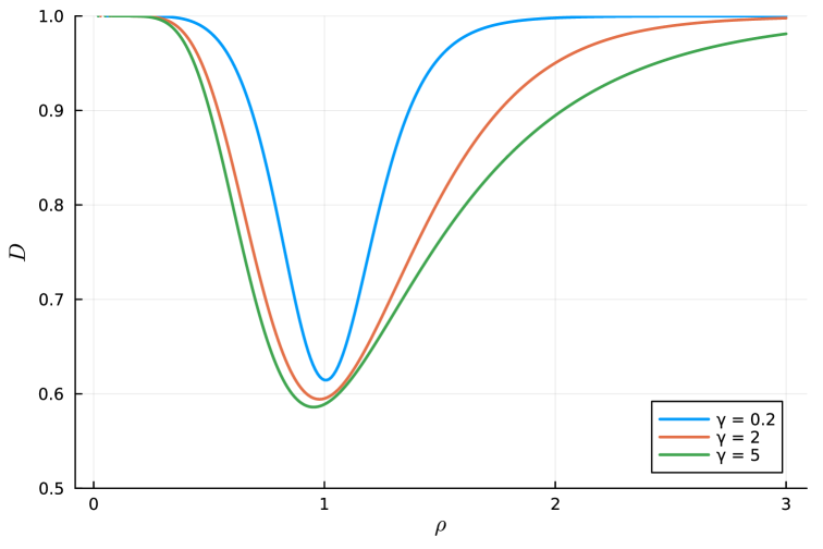
Figure 1: The asymptotic index of dispersion for M/M/$s$/K$+$M systems with $K=20$, $s=10$, and $\mu=1$. When the offered load $\rho\approx\lambda/(\mu s)$, the asymptotic variability of the output process is reduced in comparison to the Poisson process ($\mathcal{D}=1$) case.

This next example, illustrates a situation where counting thinned arrivals maybe of interest:

Example 2.

Finite population interaction upon arrival. Consider a finite population queueing system with $J$ individuals in the population, arriving, and departing from an unlimited service (infinite server) queue. An example is a small population of a certain species living on a small island and occasionally meeting at a fresh water source. As an additional individual arrives to the water source, there is a possibility of it interacting with one of the other individuals already there, or not. This probability increases as the number of individuals at the water source increases.

For this situation we set the BD and thinning parameters as,

$$\lambda_{i}=(J-i)\lambda,\qquad\mu_{i}=i\,\mu,\qquad q_{i}^{-}=0,\qquad q_{i}^{+}=\frac{i}{i+1},$$

where we note that $\lambda_{i}$ and $\mu_{i}$ in this form capture the finite population and the unlimited service.

Figure 2 presents the asymptotic index of dispersion as a function of $\lambda$ when $\mu=1$, for various population sizes, $J$. Observe that the asymptotic index of dispersion can be both greater and smaller than unity. Also note (not in figure), that as $\lambda\to\infty$ the asymptotic index of dispersion rises to $1$.

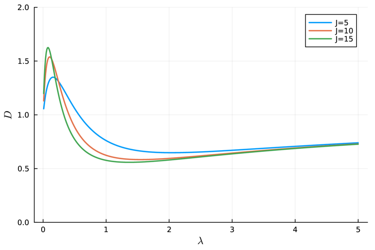
Figure 2: The asymptotic index of dispersion for a counting process of interactions upon arrival to a finite population unlimited service system.

Infinite State Calculations

The calculations in this section rely on the formal expression (2.14) for the infinite state space case. We have not presented a proof for the validity of (2.14). In particular, characterization of the conditions for which (2.14) is valid is a matter requiring further research. Nevertheless, we believe that the following infinite state space calculations are insightful as they hint at the validity of (2.14).

Example 3.

Renewal process of positive recurrent M/M/1 busy cycles. Assume $q^{+}_{i}\equiv 0$ for all $i$, $q^{-}_{1}=1$ and $q^{-}_{i}\equiv 0$ for $i\geq 2$. This is a pure death-counting process. The BD process for a simple queue has $\lambda_{i}=\lambda$, $\mu_{i}=\mu$ and $\rho:=\lambda/\mu<1$. Further, $\pi_{k}=(1-\rho)\rho^{k}$ and $1-P_{k}=\rho^{k+1}$. A busy cycle is a time interval between $Q$ exiting 0. Then (2.14) simplifies to,

$$\mathcal{D}_{\infty}=1-2(1-\rho)\rho+2\rho^{2}\sum_{k=1}^{\infty}\rho^{k}=1-2\rho\frac{1-2\rho}{1-\rho}.$$ (4.1)

Interestingly, for $\rho\in(0,\frac{1}{2})$, $\mathcal{D}<1$, for $\rho=\frac{1}{2}$, $\mathcal{D}=1$ and for $\rho\in(\frac{1}{2},1)$, $\mathcal{D}>1$. The minimum is at $\rho=\frac{1}{2}(2-\sqrt{2})\approx 0.292893$ at which point, $\mathcal{D}=4\sqrt{2}-5\approx 0.656854$. The formula of (4.1) indeed agrees with classic queueing theory results based on the so-called M/G/1 busy period functional equation (see e.g. the computation in the proof of [8, Proposition 6]). In this case, using the fact that $X=B+I$, where $B$ is the busy period r.v. and $I$ is the (independent) idle period r.v., exponentially distributed with rate $\lambda$, it is easy to obtain,

$${\mathbb{E}}[X] =\frac{1}{\mu}\frac{1}{1-\rho}+\frac{1}{\lambda}=\mu^{-1}\frac{1}{\rho(1-\rho)},$$

$${\mathbb{E}}[X^{2}] =\frac{1}{\mu^{2}}\frac{2}{(1-\rho)^{3}}+2\Big{(}\frac{1}{\mu}\frac{1}{1-\rho}\Big{)}\Big{(}\frac{1}{\lambda}\Big{)}+\frac{2}{\lambda^{2}}=2\mu^{-2}\frac{1-2\rho(1-\rho)}{\rho^{2}(1-\rho)^{3}}.$$

Combining the above gives ${\mathbb{E}}[X^{2}]/({\mathbb{E}}[X]^{2})-1$ consistent with (4.1).

Example 4.

Constant birth rates, fully counting pure-death process. Consider the infinite state space case where $\lambda_{i}=\lambda$ (constant) for all $i$, $q^{+}_{i}=0$ (all $i$), $q_{i}^{-}\equiv 1$, $\mu_{i}=\min\{i,s\}\mu$ and $\rho=\lambda/(s\mu)<1$. This is the case for output of a stable M/M/$s$ queue. By reversibility, [10], it is known that in the stationary case the output process is Poisson and hence has $\mathcal{D}=1$. Indeed using (2.14), ${\overline{\lambda}}=\lambda$ and $\Lambda_{k}=P_{k-1}$ so every product in the numerators in the sum preceding (2.14) is zero, and $\mathcal{D}=1$.

Suppose now that $q_{i}^{-}=q$ (all $i=1,2,\ldots$) for some $q$ in $(0,1)$. Then the thinning of departures is independent of the state and hence the output process is still a Poisson process. Indeed repeating the calculations (observing that ${\overline{\lambda}}=q\lambda$) we again obtain $\mathcal{D}=1$.

Example 5.

M/M/1: Thinning and counting both the input and output processes at constant probabilities. Consider again a stable M/M/1 queue with arrival rate $\lambda_{i}=\lambda$ and service rate $\mu_{i}=\mu$. Now Let $q_{i}^{+}=q^{+}$ and $q_{i}^{-}=q^{-}$ for all $i$ where $q^{-}$ and $q^{+}$ are two constants in $(0,1]$.

In this case, we have $P_{k}-\Lambda_{k}=(\pi_{k}\,q^{-})/(q^{+}+q^{-})$ which leads to

$$\mathcal{D}_{\infty}=1+H(q^{-},q^{+}),$$

where $H(q^{-},q^{+})$ is the harmonic mean of $q^{-}$ and $q^{+}$. In particular if $q^{-}=q^{+}=q$ we get $\mathcal{D}_{\infty}=1+q$.

Interestingly, when either $q^{+}=0$ or $q^{-}=0$, the counting process becomes a thinned Poisson process and we obtain $\mathcal{D}_{\infty}=\mathcal{D}=1$. However, when both the input and output processes are counted together, we have $\mathcal{D}_{\infty}>1$ due to the dependence and positive correlation between the two thinned processes.

Acknowledgements

Daryl Daley’s work done as an Honorary Professorial Associate at the University of Melbourne. The second and third author are indebted to his mentorship and collegiality throughout the work on this project. Daryl Daley, passed on 16 April 2023 and the last face to face discussion about this manuscript was a month earlier. See [15] for an insightful outline of some his scientific contributions throughout his career.

Jiesen Wang’s research has been supported by the European Union’s Horizon 2020 research and innovation programme under the Marie Sklodowska-Curie grant agreement no. 101034253, and by the NWO Gravitation project NETWORKS under grant agreement no. 024.002.003 .

References

- [1] Al Hanbali, A., Mandjes, M., Nazarathy, Y., and Whitt, W. (2011). The asymptotic variance of departures in critically loaded queues. Advances in Applied Probability 43, 243–263.
- [2] Asmussen, S. (2003). Applied Probability and Queues, second edition. Springer, New York.
- [3] Brown, M. and Solomon, H. (1975). A second-order approximation for the variance of a renewal reward process. Stochastic Processes and their Applications 3, 301–314.
- [4] Daley, D.J. (2011). Revisiting queueing output processes: a point process viewpoint. Queueing Systems 68, 395–405.
- [5] Daley, D.J., Nazarathy, Y., and van Leeuwaarden, J.S.H. (2015). BRAVO for many-server QED systems with finite buffers. Advances in Applied Probability 47, 231–250.
- [6] Eden, U.T. and Kramer, M.A. (2010). Drawing inferences from Fano factor calculations. Journal of Neuroscience Methods 190, 231–250.
- [7] Glynn, P.W. and Wang, R.J. (2023). A heavy-traffic perspective on departure process variability. Stochastic Processes and their Applications 166, 104097
- [8] Hautphenne, S., Kerner, S., Nazarathy, Y., and Taylor, P.G. (2015). The intercept term of the asymptotic variance curve for some queueing output processes. European Journal of Operational Research 24, 455–464.
- [9] He, Q. M. (2014). Fundamentals of Matrix-Analytic Methods. Springer, Vol. 365.
- [10] Kelly, F.P. (2011). Reversibility and Stochastic Networks. Cambridge University Press, Cambridge.
- [11] Nadarajah, S. and Pogány, T.K. (2018). Precise formulae for Bravo coefficients. Operations Research Letters 46, 189–192.
- [12] Nazarathy, Y. (2011). The variance of departure processes: puzzling behavior and open problems. Queueing Systems 68, 385–394.
- [13] Nazarathy, Y. and Palmowski, Z. (2022). On busy periods of the critical GI/G/1 queue and BRAVO. Queueing Systems 102, 219–225.
- [14] Nazarathy, Y. and Weiss, G. (2008). The asymptotic variance rate of finite capacity birth–death queues. Queueing Systems 59, 135–156.
- [15] Taylor, P. (2023). Daryl John Daley, 4 April 1939–16 April 2023: An internationally acclaimed researcher in applied probability and a gentleman of great kindness. Journal of Applied Probability 60, 1516–1531.