Data-Distill-Net: A Data Distillation Approach
Tailored for Reply-based Continual Learning

Abstract

Replay-based continual learning (CL) methods assume that models trained on a small subset can also effectively minimize the empirical risk of the complete dataset. These methods maintain a memory buffer that stores a sampled subset of data from previous tasks to consolidate past knowledge. However, this assumption is not guaranteed in practice due to the limited capacity of the memory buffer and the heuristic criteria used for buffer data selection. To address this issue, we propose a new dataset distillation framework tailored for CL, which maintains a learnable memory buffer to distill the global information from the current task data and accumulated knowledge preserved in the previous memory buffer. Moreover, to avoid the computational overhead and overfitting risks associated with parameterizing the entire buffer during distillation, we introduce a lightweight distillation module that can achieve global information distillation solely by generating learnable soft labels for the memory buffer data. Extensive experiments show that, our method can achieve competitive results and effectively mitigates forgetting across various datasets. The source code will be publicly available.

1 Introduction

Continual Learning (CL) (Thrun & Mitchell, 1995), also known as Lifelong Learning, is a machine learning paradigm aimed at continually learning new tasks in ever-changing environments while maintaining knowledge from old tasks. This learning approach mimics the human ability to acquire new knowledge without forgetting what has already been mastered. A key challenge of CL is catastrophic forgetting (McCloskey & Cohen, 1989), a phenomenon where the model is prone to erasing previously acquired knowledge. The root cause lies in the lack of access to data from prior tasks, causing the model to overwrite parameters containing information relevant to old tasks during the training of new ones, subsequently leading to a substantial decline in performance on earlier tasks.

To address the issue of catastrophic forgetting in CL, a variety of replay-based works (Ratcliff, 1990a; Rebuffi et al., 2017; Buzzega et al., 2020; Arani et al., 2022; Bang et al., 2021; Wu et al., 2024a) have recently emerged. These approaches consolidate previously acquired knowledge by introducing a memory buffer that retains a limited portion of old task data and replays them alongside new task data during training. For example, the earliest replay-based method, Experience Replay (ER) (Ratcliff, 1990a), employs reservoir sampling (Vitter, 1985) to randomly select samples from old tasks for storage and replay. To further refine which samples are retained, numerous coreset selection strategies have been proposed to identify more informative subset for each task. For example, certain heuristic methods concentrate on capturing the most representative samples from each class (e.g., iCaRL (Rebuffi et al., 2017), RM (Bang et al., 2021), GSS (Aljundi et al., 2019b), OCS (Yoon et al., 2021)) or those lying closer to the decision boundary (e.g., Rwalk (Chaudhry et al., 2018a), MIR (Aljundi et al., 2019a), ASER (Shim et al., 2021)).

All these methods are fundamentally based on the assumption that training on a small coreset is sufficient to minimize the empirical risk on the entire original dataset. However, due to capacity constraints, a limited memory buffer may fail to accurately approximate the stationary distribution of all previously encountered tasks, particularly when exemplars are selected using heuristic strategies (Wang et al., 2022b). Consequently, a substantial discrepancy often arises between the distribution of the stored data and that of the complete dataset from older tasks. This naturally raises the question: how can a limited buffer be used to better approximate the underlying assumption of replay-based methods?

Recent research (Liu et al., 2020; Yang et al., 2023) suggests that rather than merely selecting a subset, generating a small dataset that preserves performance on the original dataset could offer a promising alternative. This learning paradigm, often referred to as dataset distillation or dataset condensation (Wang et al., 2018), aims to compress the information from a large dataset into a compact synthetic dataset that achieves results on par with the original. In CL scenarios, since only the task $\mathcal{T}^{n}$ is accessible during learning task $n$, recent distillation-based methods (Liu et al., 2020; Yang et al., 2023) focus on compressing $\mathcal{T}^{n}$ into a small subset $\mathcal{E}^{n}$, which is then combined with the existing memory buffer $\mathcal{M}^{n-1}=\cup_{k=1}^{n-1}\mathcal{E}^{k}$ to form a new buffer, i.e., $\mathcal{M}^{n}=\mathcal{M}^{n-1}\cup\mathcal{E}^{n}$. Upon analyzing the evolution of the memory buffer, we observe that, up to task timestamp $n$, the resulting $\mathcal{M}^{n}$ ensures only intra-task information condensation, which neglects the relationships between different tasks. In other words, while $\mathcal{M}^{n}$ can effectively preserve class discrimination within each task $\mathcal{T}^{k}$ (for $k\in[n]$) , it fails to maintain class discrimination across all $n$ tasks. Consequently, this limitation prevents $\mathcal{M}^{n}$ from meeting the practical requirements of replay-based methods, which assume on training with $\mathcal{M}^{n}$ to adequately minimize the empirical risk over the entire dataset $\mathcal{T}^{[1:n]}$.

To address this challenge, this paper proposes a simple yet efficient dataset distillation framework tailored for replay-based CL methods. The framework aims to construct a memory buffer distilled not only from the current task data but also from the accumulated knowledge preserved in the previous memory buffer. Unlike current methods (Liu et al., 2020; Yang et al., 2023), our method treats the entire memory buffer as differentiable parameters at each task timestamp, enabling it to capture global information from cross-task data. To mitigate the computational overhead and overfitting risk introduced by parameterizing the entire memory buffer, we further propose a novel strategy in which only the labels of the memory buffer data are treated as learnable parameters, with these parameters generated by a unified hyper-network, Data-Distill-Net (or abbreviated as DDN). We theoretically demonstrate the feasibility of distilling global information from cross-task data via the hyper-network and empirically validate the effectiveness of our approach through extensive experiments across various settings and benchmark datasets. Our main contributions are summarized as follows:

• We propose a new dataset distillation framework tailored for CL, which maintains a learnable memory buffer capable of distilling global information from the current task data and accumulated knowledge preserved in the previous memory buffer, thereby mitigating forgetting.

• Rather than parameterizing the entire memory buffer, we further propose a light-weight distillation module, Data-Distill-Net, to generate learnable soft labels for memory buffer data, which efficiently mitigates the computational overhead and overfitting risk associated with our proposed distillation framework.

• We evaluate the proposed method on four replay-based baselines under both online and offline settings. Experimental results show that our approach effectively consolidates prior knowledge and seamlessly integrates as a plugin to enhance various replay-based baselines.

2 Related Work

2.1 Continual Learning

Classic CL can be divided into several categories including replay-based methods (Ratcliff, 1990b; Buzzega et al., 2020; Arani et al., 2022; Wu et al., 2024a; Wang et al., 2024), regularization-based methods (Li & Hoiem, 2018; Kirkpatrick et al., 2017), optimization-based methods (Lopez-Paz & Ranzato, 2017; Chaudhry et al., 2018b; Rusu et al., 2017; Wu et al., 2024b), and LoRA/prompt-based methods (Wu et al., 2025; Zhiqi et al., 2025; Piao et al., 2024; Yang et al., 2024; Wang et al., 2025). Among these, replay-based methods stand out for their competitive performance by using a memory buffer to store a small part of samples from previous tasks. One important class within replay-based methods (Buzzega et al., 2020; Arani et al., 2022) focuses on maximizing the utility of stored samples. For example, DER++ (Buzzega et al., 2020) uses knowledge distillation to effectively utilize old task data stored in the buffer, while CLSER (Arani et al., 2022) integrates a fast learning module to adapt to new tasks and a slow learning module to ensure stable integration of prior knowledge.

Other critical approaches (Rebuffi et al., 2017; Aljundi et al., 2019b; Yoon et al., 2021) focus on optimizing the quality of data stored in the memory buffer through coreset selection, which prioritizes more representative and higher-quality samples for replay. For instance, iCaRL (Rebuffi et al., 2017) employs a nearest sample mean rule for classification, and RM (Bang et al., 2021) uses interval selection based on classification uncertainty (Gal & Ghahramani, 2016). OCS (Yoon et al., 2021) selects coresets based on mini-batch gradient similarity and inter-batch gradient diversity. However, these methods rely on manually designed strategies for coreset selection, which may limit their performance in complex scenarios. To address this limitation, some approaches aim to automate coreset selection. For instance, a bi-level optimization approach (Borsos et al., 2020) dynamically adjusts coreset selection based on model performance. GCR (Tiwari et al., 2022) introduces gradient approximation to reduce computational costs, while BCSR (Hao et al., 2024) improves upon (Zhou et al., 2022) by incorporating a smoothed top-K regularization term. Compared to these methods, our method considers a learnable memory buffer that distills global information from all seen tasks, thus preserving more important knowledge.

2.2 Dataset Distillation

Dataset distillation seeks to condense a large-scale dataset into a smaller synthetic dataset, such that a model trained on this condensed dataset performs comparably to one trained on the full dataset (Wang et al., 2018). This process involves optimizing the synthetic dataset to approximate the training dynamics of the full dataset, enabling the distilled data to achieve similar effects with fewer training steps.

Gradient-based methods (Zhao et al., 2020; Zhao & Bilen, 2021; Lee et al., 2022; Jiang et al., 2023; Kim et al., 2022; Zhang et al., 2023) focus on aligning the gradients between the original and synthetic datasets during training. For example, DC (Zhao et al., 2020) formulates the objective as a gradient matching problem, while DCC (Lee et al., 2022) introduces a new gradient matching distance metric that incorporates class-discriminative features. MTT (Cazenavette et al., 2022), a multi-step parameter-based method (Li et al., 2024; Cui et al., 2023), tracks the training trajectory over multiple steps to improve alignment. On the other hand, distribution-based methods focus on aligning feature statistics between the synthetic and original datasets. For instance, DM (Zhao & Bilen, 2023) employs Maximum Mean Discrepancy (Gretton et al., 2012) to match feature distributions, while (Wang et al., 2022a) ensures consistency in feature statistics extracted by each network layer for synthetic and real samples. Despite their effectiveness, existing dataset distillation methods still face challenges in replay-based CL. Specifically, distillation samples from old tasks may be lost during memory buffer updates, disrupting the data distribution. Moreover, directly optimizing synthetic samples incurs significant computational costs. To address these issues, we propose a continual label distillation process that leverages a bi-level optimization mechanism. This approach preserves data distribution and reduces computational overhead, offering a more efficient solution for CL.

3 Preliminaries

Consider a classification model $f_{\theta}$ trained on $N$ sequentially arriving tasks, denoted as $\{\mathcal{T}^{1},\mathcal{T}^{2},...,\mathcal{T}^{N}\}$, where the $n$-th task is represented as $\mathcal{T}^{n}=\{X^{n},Y^{n}\}$, with $X^{n}$ and $Y^{n}$ being the input data and corresponding labels, respectively. For the $n$-th task, the ideal objective of CL is to minimize the following empirical risk,

$$\theta^{*}=\arg\min_{\theta}\mathcal{L}(f_{\theta};\mathcal{T}^{[1:n]}),$$ (1)

where $\theta^{*}$ denote the optimal model weights, $\mathcal{L}$ refer to the cross-entropy loss, and $\mathcal{T}^{[1:n]}=\cup_{k=1}^{n}\mathcal{T}^{k}$ means the all seen $n$ tasks. When learning the $n$-th task, memory constraints and privacy concerns restrict access to the complete set of examples from the previous tasks $\mathcal{T}^{1:n-1}$. To mitigate this limitation, replay-based CL methods leverage a small memory buffer $\mathcal{M}^{n-1}=\mathcal{E}^{[1:n-1]}$, where $\mathcal{E}^{k}\subset\mathcal{T}^{k}$ (with $|\mathcal{E}^{k}|\ll|\mathcal{T}^{k}|,k\in[n-1]$) is a subset of examples sampled from $\mathcal{T}^{k}$. Using this buffer, the training objective in Eqn. (1) can be approximated as follows,

$$\theta^{*}=\arg\min_{\theta}\mathcal{L}(f_{\theta};\mathcal{M}^{n-1}\cup\mathcal{T}^{n}).$$ (2)

Dataset distillation in CL. Similar to traditional reply-based methods, recent distillation methods (Liu et al., 2020; Yang et al., 2023) also maintain a small memory buffer $\mathcal{M}^{n-1}=\mathcal{E}^{[1:n-1]}$ to reply when learning task $n$. In contrast, these methods distill each $\mathcal{E}^{k}$ from $\mathcal{T}^{k}$ at the timestamp $k$. Specifically, this can be formulated as the following bi-level optimization problem:

$$\mathcal{E}^{k} =\arg\min_{\mathcal{E}^{k}_{tmp}}\mathcal{L}(f_{\theta^{*}(\mathcal{E}_{tmp}^{k})};\mathcal{T}^{k})$$ (3)

 s.t. $$\quad\theta^{*}(\mathcal{E}^{k}_{tmp})=\arg\min_{\theta}\mathcal{L}(f_{\theta};\mathcal{E}^{k}_{tmp}),$$

where the inner loop trains a temporary classifier model $f_{\theta}$ on the synthetic data $\mathcal{E}^{k}_{tmp}$ (treated as a hyper-parameter), and the outer loop uses the entire data $\mathcal{T}^{k}$ as a validation set to optimize $\mathcal{E}^{k}_{tmp}$. It shows that, each $\mathcal{E}^{k}$ in $\mathcal{M}^{n-1}$ only condenses intra-task information within task $k$, such that the resulting buffer neglects the relationships between different tasks. To illustrate this, we consider a three-task CL scenario and demonstrate the evolution of the memory buffer in Fig. 1(a). Throughout the CL process, we can see that the subsets from different tasks do not interact, implying that they are treated as independently distributed across tasks.

4 Method

In this section, we propose a new dataset distillation framework tailored for CL. Rather than distilling information for individual tasks, as described in Eqn. (3) and Fig. 1(a), our approach explicitly captures inter-task relationships.

Figure 1: Comparison between traditional dataset distillation (a) and our proposed method (b). At the $n$-th task $\mathcal{T}^{n}$, the distilled data $\mathcal{E}^{n}$ in the traditional approach contains only task-specific information from $\mathcal{T}^{n}$, while the samples in $\mathcal{M}^{n}$ fail to capture inter-task relationships as illustrate in  (a). In contrast, our method distills samples for the memory buffer $\mathcal{M}^{n}$ from both the current task $\mathcal{T}^{n}$ and the previous buffer $\mathcal{M}^{n-1}$, thereby preserving correlations across tasks as shown in (b).

4.1 Tailored Distillation Framework for CL

Unlike traditional dataset distillation methods exclusively for individual tasks, our proposed framework maintains a learnable memory buffer to distill the global information from the current task data and accumulated knowledge preserved in the previous memory buffer. As a result, it can effectively capture the relationships among sequential tasks, making it highly suitable for continual learning.

Specifically, when learning the $n$-th task $\mathcal{T}^{n}$, we directly parameterize the memory buffer $\mathcal{M}^{n}_{tmp}$ as learnable parameters, which are then utilized to distill both the current task data $\mathcal{T}^{n}$ and the existing buffer $\mathcal{M}^{n-1}$. This process is realized through a bi-level optimization strategy, as follows:

$$\mathcal{M}^{n} =\arg\min_{\mathcal{M}^{n}_{tmp}}\mathcal{L}(f_{\theta^{*}(\mathcal{M}^{n}_{tmp})};\mathcal{M}^{n-1}\cup\mathcal{T}^{n})$$ (4)

 s.t. $$\quad\theta^{*}(\mathcal{M}^{n}_{tmp})=\arg\min_{\theta}\mathcal{L}(f_{\theta};\mathcal{M}^{n}_{tmp}),$$

where the inner loop trains a temporary classifier $f_{\theta}$ on the learnable buffer $\mathcal{M}^{n}_{tmp}$, which is treated as a hyperparameter, to obtain an optimal parameter $\theta^{*}$, and the outer loop utilizes the combined global information $\mathcal{M}^{n-1}\cup\mathcal{T}^{n}$ from all seen $n$ task as a validation set to optimize $\mathcal{M}^{n}_{tmp}$. By optimizing Eqn. (4), we obtain the desired buffer $\mathcal{M}^{n}$, which corresponds to the optimal $\mathcal{M}^{n}_{tmp}$.

As illustrated in Fig. 1 (b), our proposed continuous distillation strategy, described in Eqn. (4), distills $\mathcal{M}^{n}$ by considering not only the current task and previously learned tasks but also the relationships between them after completing the training of each task. This approach avoids the loss of important distilled samples in the buffer $\mathcal{M}$ during updates through reservoir sampling, as illustrated in Fig.1(a). By distilling the buffer and the current task simultaneously, rather than randomly replacing the samples stored in $\mathcal{M}$, we can preserve the core information from both sources while effectively extracting their global task relationships, which are empirically demonstrated to be critical in Sec. 6.

4.2 Efficient Distillation with Data-Distill-Net

To capture global information from cross-task data, Eqn. (4) parametrizes the entire memory buffer as differentiable parameters during each continual learning phase. However, this strategy introduces significant computational overhead and increases the risk of overfitting during buffer optimization. To address these challenges, we further propose a lightweight distillation module, Data-Distill-Net (DDN), to ensure effective distillation of global information across tasks while mitigating the computational overhead and overfitting risks associated with full buffer parameterization. For simplicity, we denote the memory buffer as $\mathcal{M}^{n}=\{X_{buf}^{n},Y_{buf}^{n}\}$ with $Y_{buf}^{n}$ representing the sets of one-hot labels corresponding to $X_{buf}^{n}$.

Instead of directly parameterizing the entire $\mathcal{M}^{n}$ in Eqn. (4), the DDN module first constructs $\mathcal{M}^{n}$ using existing replay-based methods, such as the commonly used reservoir sampling (Vitter, 1985). It then treats the soft version of $Y^{n}_{buf}$ as learnable parameters and employs a unified hyper-network $\mathcal{G}_{\omega}^{n}$ to generate these parameters, where $\omega$ denotes its parameters and $n$ represents the current CL phase. Specifically, this can be formulated as

$$\tilde{Y}^{n}_{buf}(\omega)=\mathcal{G}^{n}_{\omega}(X^{n}_{buf}).$$ (5)

Furthermore, the parameter $\omega$ of $\mathcal{G}_{\omega}^{n}$ is treated as a hyper-parameter and optimized through a bi-level optimization problem similar to Eqn. (4). It can be expressed as

$$\omega^{*} =\arg\min_{\omega}\mathcal{L}\bigl{(}f_{\theta^{*}(\omega)};\{X_{buf}^{n-1},Y_{buf}^{n-1}\}\cup\mathcal{T}^{n}\bigr{)}$$ (6)

 s.t. $$\quad\theta^{*}(\omega)=\arg\min_{\theta}\mathcal{L}\bigl{(}f_{\theta};\{X^{n}_{buf},\tilde{Y}^{n}_{buf}(\omega)\}\bigr{)}.$$

Once the optimal $\omega^{*}$ is obtained after learning $\mathcal{T}^{n}$, we only need to retain $X_{buf}^{n}$ and the lightweight $\mathcal{G}_{\omega^{*}}^{n}$ in the buffer, which are subsequently utilized to replay global information from the preceding $n$ tasks, by forming a learnable buffer $\mathcal{M}^{n}=\bigl{\{}{X_{buf}^{n},\mathcal{G}_{\omega^{*}}^{n}(X_{buf}^{n})}\bigr{\}}$, during the learning of $\mathcal{T}^{n+1}$.

The success of our proposed distillation framework relies on Data-Distill-Net’s ability to extract global information from $\mathcal{T}^{n}\cup\mathcal{M}^{n-1}$. While it employs a hypernetwork-driven parameterization to generate adaptive soft-label distributions for the memory buffer, rather than direct parametric optimization as in Eqn. (4), we have theoretically proven its functional equivalence to the direct parameterization through gradient signal alignment. The detailed proof is provided in Sec. 5.

4.3 Data-Distill-Net as a Plugin for Replay-based CL

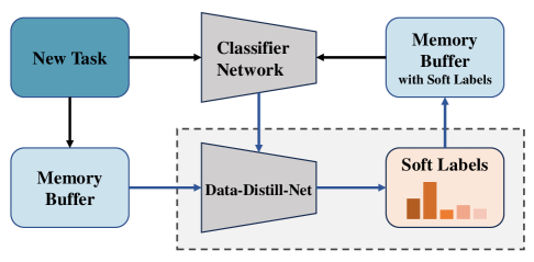
Figure 2: Overall framework of the proposed DDN. By generating refined soft labels for buffer samples, DDN enhances the classifier’s training, thereby mitigating catastrophic forgetting of prior task knowledge. The training algorithms for the classifier and DDN are detailed in Algorithm 1 and Algorithm 2, respectively.

As aforementioned, our proposed distillation framework does not change the construction or storage manner of the memory buffer data. Instead, it merely introduces a lightweight DDN to condense global information. Therefore, this distillation module can be integrated as a plug-in with any existing replay-based CL method, as illustrated in Fig. 2 and Algorithm 1.

Specifically, during the learning of $\mathcal{T}^{n}$, given the retained buffer data $X_{buf}^{n-1}$ and the DDN module $\mathcal{G}_{\omega}^{n-1}$, we first apply DDN to generate soft labels $\tilde{Y}_{buf}^{n-1}(\omega)=\mathcal{G}_{\omega}^{n-1}(X_{buf}^{n-1})$ for these buffer data. We then update the classifier network $f_{\theta}$ using the resulting learnable buffer $\mathcal{M}^{n-1}=\{X_{buf}^{n-1},\tilde{Y}_{buf}^{n-1}\}$ by minimizing the following empirical risk:

$$\mathcal{L}(f_{\theta};\mathcal{T}^{n}\cup\mathcal{M}^{n-1})=\mathcal{L}(f_{\theta};\mathcal{T}^{n})+\alpha\mathcal{L}(f_{\theta};\mathcal{M}^{n-1}),$$ (7)

where $\alpha$ is a hyper-parameter controlling the trade-off between learning new tasks and retaining previously acquired knowledge. Subsequently, we optimize the bi-level optimization problem Eqn. (6) to update the DDN module. Due to space constraints, the optimization procedure of Eqn. (6) is detailed in Appendix A.

Note that DDN is only enabled during the training phase. During testing, the trained classifier network is used directly for predictions, so there is no additional computational burden during testing.

Architectural designs of DDN. The proposed DDN $\mathcal{G}_{\omega}^{n}$ is implemented as a Multi-Layer Perceptron (MLP) with two hidden layers, each comprising 200 units followed by a ReLU activation function. For an input $x$, the DDN takes the predicted probabilities from classifier network $f_{\theta}$ (with gradients stopped) and outputs a soft label $\tilde{y}$. As the inputs of $\mathcal{G}_{\omega}$ depends on the classifier network, it might make $\mathcal{G}_{\omega}$ suffer from forgetting when encountering new tasks. To address this issue, we employ an Exponential Moving Average (EMA) to generate soft labels by $\mathcal{G}_{\omega}$. Specifically, at the end of the $(n-1)$-th task, we save $\mathcal{G}_{\omega}^{n-1}$ as $\mathcal{G}_{old}$, which is used as a ‘cached checkpoint’ to smooth the outputs of $\mathcal{G}_{\omega}^{n}$ in the current $n$-th task. Consequently, the soft label generated by DDN in Eqn. (5) can be reformulated as

$$\tilde{Y}^{n}_{buf}(\omega)=(1-\beta)\mathcal{G}^{n}_{\omega}(X^{n}_{buf})+\beta\mathcal{G}_{old}(X^{n}_{buf}),$$ (8)

where $\beta\in[0,1]$ is the EMA weight of $\mathcal{G}_{old}$.

In this work, we additionally add the corresponding one-hot label to $\tilde{y}$ and then apply normalization to ensure that it constitutes a valid probability distribution. Despite its simple structure, DDN leverages its universal approximation capability (Haykin, 1998) to effectively capture and represent complex relationships between different classes.

Algorithm 1 Training of classifier network

 Input: current task $\mathcal{T}^{n}$, classifier network $f_{\theta}$, DDN $\mathcal{G}_{\omega}^{n-1}$, memory buffer $\mathcal{M}^{n-1}$, max iterations K

 for $i=0$ to K do

  $\mathcal{B}^{n}\!=\!\{X^{n},Y^{n}\}\!\leftarrow\!$ SampleMiniBatch($\mathcal{T}^{n}$)

  $\mathcal{B}^{n-1}_{buf}\!=\!\{X^{n-1}_{buf},Y^{n-1}_{buf}\}\!\leftarrow\!$ SampleMiniBatch($\mathcal{M}^{n-1}$)

  Generate soft-labels $\tilde{Y}_{buf}^{n-1}=\mathcal{G}_{\omega}^{n-1}(X_{buf}^{n-1})$

  Update $\theta$ of classifier network by minimize Eq. (7)

  Update DDN by Algorithm 2

 end for

Algorithm 2 Training of DDN

 Input: current task $\mathcal{T}^{n}$, memory buffer $\mathcal{M}^{n-1}$, max iterations K

 for $i=0$ to K do

  # Inner loop

  $\mathcal{B}^{in}\!=\!\{X^{in},Y^{in}\}\!\leftarrow\!$ SampleMiniBatch($\mathcal{M}^{n}$)

  Generate soft labels $\tilde{Y}^{in}(\omega)=\mathcal{G}_{\omega}^{n-1}(X^{in})$

  Update $\theta(\omega)$ of classifier network by minimizing $\mathcal{L}(f_{\theta};\{X^{in},Y^{in}\})+\alpha\cdot\mathcal{L}(f_{\theta};\{X^{in},\tilde{Y}^{in}(\omega)\})$

  # Outer loop

  $\mathcal{B}^{out}\!=\!\{X^{out},Y^{out}\}\!\!\leftarrow\!\!$ SampleMiniBatch($\mathcal{M}^{n-1}\!\cup\!\mathcal{T}^{n}$)

  Update $\omega$ of DDN by minimizing $\mathcal{L}(f_{\theta(\omega)};\mathcal{B}^{out})$

 end for

5 Theoretical Analysis

In this section, we establish the theoretical connections between two memory buffer parameterization paradigms. Whereas Eqn. (4) implements direct parametric optimization by treating the entire memory buffer as learnable parameters, Eqn. (6) proposes a hypernetwork-driven parameterization that generates adaptive soft-label distributions for memory entries. To formalize this equivalence, we first demonstrate that our bi-level framework Eqn. (4) corresponds to the gradient-matching formulation below.

Theorem 5.1.

Let $\nabla_{\theta}\mathcal{L}(f_{\theta};\mathcal{M}^{n})$ be the gradients w.r.t. $\theta$ on the parameterized memory buffer $\mathcal{M}^{n}$, and $\nabla_{\theta}\mathcal{L}(f_{\theta};\mathcal{M}^{n-1}\cup\mathcal{T}^{n})$ be the gradients w.r.t. $\theta$ on the current task $\mathcal{T}^{n}$ and the previous buffer $\mathcal{M}^{n-1}$. The bi-level framework in Eqn. (4) is equivalent to minimizing the following empirical risk:

$$\min_{\mathcal{M}^{n}}-\bigl{\langle}\nabla_{\theta}\mathcal{L}(\theta;\mathcal{M}^{n}),\nabla_{\theta}\mathcal{L}(\theta;\mathcal{M}^{n-1}\cup\mathcal{T}^{n})\bigr{\rangle}.$$ (9)

Next, we show that the bi-level framework in Eqn. (6) is equivalent to the following gradient-matching formulation.

Theorem 5.2.

Let $\nabla_{\theta}\mathcal{L}(f_{\theta};\mathcal{M}^{n})$ be the gradients w.r.t. $\theta$ on the learnable memory buffer $\mathcal{M}^{n}=\bigl{\{}{X_{buf}^{n},\mathcal{G}_{\omega}^{n}(X_{buf}^{n})}\bigr{\}}$, and $\nabla_{\theta}\mathcal{L}(f_{\theta};\mathcal{M}^{n-1}\cup\mathcal{T}^{n})$ be the gradients w.r.t. $\theta$ on the current task $\mathcal{T}^{n}$ and the previous buffer $\mathcal{M}^{n-1}$. The bi-level framework in Eqn. (6) is equivalent to minimizing the following empirical risk:

$$\min_{\omega}-\bigl{\langle}\nabla_{\theta}\mathcal{L}(\theta;\mathcal{M}^{n}),\nabla_{\theta}\mathcal{L}(\theta;\mathcal{M}^{n-1}\cup\mathcal{T}^{n})\bigr{\rangle}.$$ (10)

Theorem 9 and  10 demonstrate that the direct parametric optimization approach in Eqn. (4) and the hypernetwork-driven parameterization method in Eqn. (6) play analogous roles throughout the distillation process. Specifically, once both optimization objectives achieve their optimums, we have $\nabla_{\theta}\mathcal{L}\bigl{(}f_{\theta};\{X_{buf}^{n},\mathcal{G}^{n}_{\omega}\}\bigr{)}\simeq\nabla_{\theta}\mathcal{L}(\theta;\mathcal{M}^{n-1}\cup\mathcal{T}^{n})\simeq\nabla_{\theta}\mathcal{L}\bigl{(}f_{\theta};\mathcal{M}^{n}\bigr{)}$. This demonstrates that our method significantly reduces computational overhead by leveraging hypernetwork-driven parameterization instead of direct parametric optimization while still achieving the same optimum.

Table 1: Comparison results on three datasets under the online continual learning setting, evaluated by ACC and FM. Gray cells represent our method applied to four baselines.

	Split CIFAR-10				Split CIFAR-100				Split Tiny-ImageNet
	M=0.2K		M=0.5K		M=2K		M=5K		M=2K		M=5K
Method	ACC $\uparrow$	FM $\downarrow$	ACC $\uparrow$	FM $\downarrow$	ACC $\uparrow$	FM $\downarrow$	ACC $\uparrow$	FM $\downarrow$	ACC $\uparrow$	FM $\downarrow$	ACC $\uparrow$	FM $\downarrow$
LUCIR (Hou et al., 2019)	23.59	35.59	24.63	31.89	8.28	16.07	12.31	14.02	4.47	20.40	5.29	20.28
iCaRL (Rebuffi et al., 2017)	40.49	26.84	44.50	24.87	9.13	7.79	9.13	8.14	4.03	4.93	4.03	5.15
BiC (Wu et al., 2019)	27.71	66.45	35.47	47.92	16.32	36.70	20.89	32.33	5.43	40.14	7.50	38.52
Mnemonics (Liu et al., 2020)	37.08	38.27	43.12	29.88	22.93	27.29	23.82	28.05	15.38	26.72	16.91	24.98
LoDM (Yang et al., 2023)	30.57	17.84	29.22	19.57	14.78	11.20	15.02	10.95	4.43	9.08	4.83	10.72
ER (Ratcliff, 1990a)	36.05	49.99	44.34	36.90	21.23	33.99	23.78	33.1	15.35	31.45	16.86	30.76
ER DDN (ours)	41.93	35.28	48.11	30.07	23.41	30.08	24.48	30.25	15.13	28.06	17.14	28.9
DER++ (Buzzega et al., 2020)	41.54	39.49	49.11	34.24	17.90	43.76	17.95	44.54	11.64	40.69	11.47	41.44
DER++ DDN (ours)	42.82	37.26	49.48	28.18	21.92	35.59	22.29	37.22	13.84	35.46	15.54	34.44
CLSER (Arani et al., 2022)	39.03	48.49	44.58	37.31	21.65	36.15	23.40	35.38	14.79	33.19	16.64	32.79
CLSER DDN (ours)	40.95	40.06	47.37	29.74	22.80	31.48	25.05	30.44	15.16	32.87	17.61	28.93
ER-ACE (Caccia et al., 2021)	42.81	17.32	47.02	17.53	25.74	7.26	28.53	6.13	17.64	7.58	20.37	5.53
ER-ACE DDN (ours)	43.37	17.60	50.02	14.50	25.94	8.71	28.73	7.73	18.25	9.81	21.02	7.02

6 Experiments

To verify the effectiveness of our method DDN, we compared it with several current state-of-the-art CL baselines under different experimental setups including online and offline settings. Additionally, we conducted a series of ablation experiments to demonstrate the rationale of our method.

6.1 Experimental Settings

Datasets: Our experiments are conducted on three commonly used CL datasets following (Buzzega et al., 2020): Split CIFAR-10 (Krizhevsky et al., 2009), Split CIFAR-100, and Split Tiny-ImageNet (Pouransari & Ghili, 2014). Specifically, we split CIFAR-10 into 5 binary classification tasks. Both CIFAR-100 and Tiny-ImageNet are divided into 10 tasks, with 10 classes and 20 classes per task, respectively. See Appendix C for details.

Metrics: To fairly evaluate our approach and other comparison methods, we employ the following two metrics in all experiments.

• Average Accuracy (ACC $\uparrow$): The average accuracy measures the overall CL classification ability, i.e., $\mathrm{ACC}=\frac{1}{T}\sum_{i=t}^{T}A_{t,T}$, where $A_{t,T}$ represents the test accuracy of the model on the $t$-th task $\mathcal{T}^{t}$ after the training of all $T$ tasks. Additionally, $\uparrow$ indicates that higher is better.

• Forgetting Measure (FM $\downarrow$): FM measures the average forgetting of each task, where the lower FM ($\downarrow$) is better. Specifically, FM calculates the average difference between the best performance during the whole CL stage $A^{*}_{t}$ and the final performance $A_{t,T}$, i.e., $\mathrm{FM}=\frac{1}{T}\sum_{i=t}^{T}A^{*}_{t}-A_{t,T}$.

Comparison methods: The proposed DDN can be easily plugged into various rehearsal-based CL methods and further improve their performance, such as ER (Ratcliff, 1990a), DER++ (Buzzega et al., 2020), CLSER (Arani et al., 2022), and ER-ACE (Caccia et al., 2021). To verify the strength of our method, we also compare the performance with several representative rehearsal methods, i.e., LUCIR (Hou et al., 2019), iCaRL (Rebuffi et al., 2017), BiC (Wu et al., 2019), and two dataset distillation CL methods LoDM (Yang et al., 2023) and Mnemonics (Liu et al., 2020), whose memory buffer applied distillation samples. Details of comparison methods please refer to Appendix C.

Implementation details: We focus primarily on online and offline CL settings. Specifically, in online CL, data arrives sequentially, and each sample is trained only once, except for those stored in a memory buffer, making it more challenging as models must learn quickly while mitigating forgetting. In contrast, offline CL allows storing the current task samples and training multiple times, leading to more stable performance, though catastrophic forgetting remains a key challenge. In our experiments, we take the average results of 10 runs and 3 runs to alleviate random factors for online and offline CL, respectively. We adopt ResNet-18 as backbone follow (Buzzega et al., 2020) and train all methods by stochastic gradient descent (SGD) optimizer. For our DDN, we use Adam (Kingma & Ba, 2014) optimizer with the learning rate as 0.001 for Split CIFAR-10, 0.01 for Split CIFAR-100, and 0.0001 for Split Tiny-ImageNet. More implementation details are shown in Appendix C.

6.2 Results of Online and Offline CL

Online CL. Table 1 shows the ACC and FM results for our method and all comparison methods. Note that our approach has been applied to four different rehearsal-based CL baselines, marked as ‘DDN’ with gray cells in the table. From Table 1, it is evident that our method improves the classification accuracy of the corresponding baseline while significantly reducing forgetting. For example, our ER DDN improves the ACC of the baseline ER by $5.88\%$ on Split CIFAR-10 with 0.2K memory buffer samples. Even for ER-ACE with relatively lower FM, our method can further improve the classification accuracy from a global perspective and produce a comparable FM. These results demonstrate that the proposed method effectively distills knowledge from all tasks into DDN by generating soft labels, leading to better CL performance. For a fair comparison with other dataset distillation CL methods, we also applied LoDM and Mnemonics to ER. LoDM performs poorly in online CL due to its reliance on excessive iterations to optimize condensed data samples. Mnemonics, which initializes synthetic data as real images from the training set, offers a slight improvement over ER but still falls short of our method. These results demonstrate that our distillation framework is better suited for CL tasks, significantly reducing computational costs while enhancing baseline performance.

Table 2: Comparison results on three datasets under the offline continual learning setting, evaluated by ACC and FM. Gray cells represent our method applied to four baselines.

	Split CIFAR-10				Split CIFAR-100				Split Tiny-ImageNet
	M=0.2K		M=0.5K		M=2K		M=5K		M=2K		M=5K
Method	ACC $\uparrow$	FM $\downarrow$	ACC $\uparrow$	FM $\downarrow$	ACC $\uparrow$	FM $\downarrow$	ACC $\uparrow$	FM $\downarrow$	ACC $\uparrow$	FM $\downarrow$	ACC $\uparrow$	FM $\downarrow$
ER (Ratcliff, 1990a)	54.91	48.43	65.31	35.45	39.37	53.62	50.05	40.17	18.71	64.77	27.58	54.01
ER DDN (ours)	58.93	43.24	68.56	29.57	46.32	43.45	56.57	30.63	22.93	47.71	31.02	42.40
DER++ (Buzzega et al., 2020)	64.59	34.99	73.31	23.45	53.04	32.56	60.45	23.39	32.22	42.34	39.88	31.50
DER++ DDN (ours)	65.73	31.34	73.96	20.01	52.65	33.57	59.85	25.20	32.42	40.18	39.37	30.04
CLSER (Arani et al., 2022)	55.25	47.14	69.05	28.42	44.84	46.13	54.71	34.26	23.75	58.75	30.93	50.70
CLSER DDN (ours)	57.34	42.00	69.79	27.88	48.46	37.34	55.85	27.76	24.97	53.69	35.58	40.95
ER-ACE (Caccia et al., 2021)	64.35	18.38	71.95	14.44	50.29	28.01	56.34	21.56	32.37	36.42	38.92	28.65
ER-ACE DDN (ours)	66.12	19.25	72.20	14.96	51.44	30.91	59.76	22.44	32.19	43.23	37.67	39.37

Offline CL. Different from online CL, models in offline CL typically achieve better and more stable results, though the forgetting issue remains pronounced. Table 2 presents the performance of our approach and comparison methods in the offline CL setting. From these results, our method significantly improves ACC and reduces FM across almost all datasets and baselines. For example, on the CIFAR-100 dataset with 2K buffer samples, our method improves by $6.95\%$ compared to the baseline. For ER-ACE, our method also enhances the accuracy with comparable FM. These superior results suggest that our DDN effectively captures and transfers knowledge from all tasks. Therefore, with our distillation framework and buffered soft labels, most rehearsal-based CL methods can be further improved in both online and offline settings.

6.3 Discussion

Comparison with other soft label methods: As aforementioned, we distill information from all tasks into DDN by generating learnable soft lables. To demonstrate the superiority of the distilled soft label, we compare our approach with other soft label methods based on ER in Table 3. First, we create random soft labels by adding uniform noise to hard labels with normalization, referred to as ‘RANDOM’ in Table 3. Such random soft labels do not provide additional useful information and even harm baseline performance. Then we evaluate label smoothing (Yuan et al., 2020) with different smoothing strength, denoted as ‘ER LS’. This approach suffers from instability during CL training and struggles to improve baseline. In contrast, our method leads to significant improvements, highlighting the effectiveness of the soft labels generated by our distillation framework.

Table 3: The online CL comparison results of our method and other soft label methods on Split CIFAR-10 with various buffer sizes.

	Split CIFAR-10
	M=0.2K		M=0.5K
Method	ACC $\uparrow$	FM $\downarrow$	ACC $\uparrow$	FM $\downarrow$
ER	36.05	49.99	44.34	36.90
RANDOM	33.47	55.64	43.85	40.56
ER LS    ($\epsilon$=0.1)	35.46	50.72	45.04	37.25
ER LS    ($\epsilon$=0.5)	34.24	52.96	42.59	41.87
ER L2Y	37.60	42.83	44.44	37.10
ER DDN (ours)	41.93	35.28	48.11	30.07

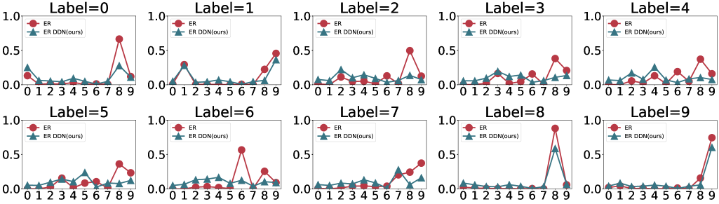
Figure 3: Under online CL, comparison of the predicted probability distributions for different class samples between ER and ER DDN(ours) on Split CIFAR-10 with buffer size M = 0.2K.

Furthermore, to verify the strength of $\mathcal{G}_{\omega}$, we directly optimize soft labels of memory buffer samples by our distillation framework as ‘ER L2Y’. While this method also improves the performance of ER, it cannot outperform our method with the $\mathcal{G}_{\omega}$, indicating the importance of this module.

Probability distribution predicted by DDN: To figure out the effect of our proposed DDN on classifier network training, under the online CL setting, we calculate the probability distribution of each class predicted by ER and our ER DDN after the whole CL training of Split CIFAR-10 with M = 0.2K in Fig. 3. For the old classes of previous tasks (i.e., Label=$0,\cdots,7$), the predicted probabilities are seriously biased toward the new classes (i.e., Label=$8,9$). In contrast, our method significantly corrects this bias and enhances the predicted probabilities of the ground truth class. On the other hand, for the new classes (i.e., Label=$8,9$), our proposed ER DDN decreases prediction confidence for these new class samples without loss of classification accuracy. Therefore, our method can automatically adapt to CL distributions by distilling knowledge from all tasks, and thus accelerate network training to achieve better performance.

Effect of small buffer size: To further investigate the effectiveness of our method in scenarios with small buffer sizes, we apply the proposed DDN to four baselines on Split CIFAR-10, as shown in Table 4. When the buffer size is M = 0.05K, our method ER DDN improves the ACC of the baseline ER by approximately $4.1\%$ and reduces FM by around $12.03\%$. These results demonstrate that our method can effectively extract and distill information from training samples across all tasks into the limited memory buffer, significantly enhancing the performance of the corresponding rehearsal baselines in memory-constrained scenarios.

Table 4: Under online CL, comparison results of our method and corresponding baselines on Split CIFAR-10 with small buffer sizes.

	Split CIFAR-10
	M=0.05K		M=0.1K
Method	ACC $\uparrow$	FM $\downarrow$	ACC $\uparrow$	FM $\downarrow$
ER (Ratcliff, 1990a)	22.44	74.46	28.08	61.30
ER DDN (ours)	26.51	62.43	34.54	45.84
DER++ (Buzzega et al., 2020)	30.11	57.91	36.21	49.66
DER++ DDN (ours)	31.52	51.82	37.19	45.85
CLSER (Arani et al., 2022)	25.53	67.46	30.58	54.59
CLSER DDN (ours)	28.08	55.93	34.77	45.90
ER-ACE (Caccia et al., 2021)	33.77	22.73	36.72	21.19
ER-ACE DDN (ours)	34.15	21.47	39.24	19.49

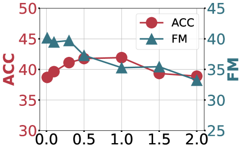
Figure 4: Under online CL, ACC and FM of different $\alpha$ and $\beta$ of our method on Split CIFAR-10 with buffer size M = 0.2K. (a) Effect of $\alpha$ with fixed $\beta=0.9$. (b) Effect of $\beta$ with fixed $\alpha=1.0$.

Effect of $\alpha$ and $\beta$: In our distillation framework, $\alpha$ and $\beta$ are key hyperparameters to control the strength of DDN and the effect of the old generator in EMA, respectively. In Fig. 4, we illustrate the effect of varying $\alpha$ and $\beta$ on Split CIFAR-10 with M = 0.2K. Our method achieves the highest ACC and a relatively lower FM at $\alpha=1.0$, indicating that our soft label loss is crucial in the classifier network training. Additionally, a larger $\alpha$ results in lower accuracy, likely because the model still relies on hard labels to provide sufficient confidence for classification. Furthermore, with $\alpha=1.0$, our method performs best when $\beta=0.9$, suggesting that the old $\mathcal{G}_{old}$ plays an important role in alleviating forgetting and improving performance.

7 Conclusion

The previous dataset distillation methods applied in the continual learning (CL) problem typically ignored the correlation between each task. To tackle this challenge, we propose a new dataset distillation framework tailored for CL, which maintains a learnable memory buffer to distill global information from all seen tasks. Furthermore, we parameterize a Data-Distill-Net (DDN) to distill global information by generating learnable soft labels for memory buffer samples, reducing the computational burden and overfitting risks during the CL training and distillation stage. We plug the designed DDN in four rehearsal-based CL baselines and the experiments have demonstrated the effectiveness of DDN under both online and offline settings.

Impact Statement

This paper aims to advance the field of Machine Learning. Specifically, we propose a novel distillation method tailored for CL, which offers significant advantages by reducing memory and computational requirements, thereby enhancing the accessibility of machine learning models in resource-constrained environments. On the flip side, these benefits might come with potential ethical and societal challenges if not properly managed. The data compression process might unintentionally exclude rare or minority examples, thereby reinforcing existing biases and diminishing fairness in applications. As a result, it is essential for practitioners to ensure transparency in how distilled datasets are created and evaluated, as well as to conduct rigorous assessments to guarantee that diverse populations are adequately represented.

Supplementary Materials
Data-Distill-Net: A Data Distillation Approach
Tailored for Reply-based Continual Learning

Appendix A Optimization of Eqn. (6)

We first recall Eqn. (6) in the main text, representing our proposed distillation framework tailored for continual learning, which can be represented as follows:

$$\omega^{*} =\arg\min_{\omega}\mathcal{L}\bigl{(}f_{\theta^{*}(\omega)};\{X_{buf}^{n-1},Y_{buf}^{n-1}\}\cup\mathcal{T}^{n}\bigr{)}$$

 s.t. $$\quad\theta^{*}(\omega)=\arg\min_{\theta}\mathcal{L}\bigl{(}f_{\theta};\{X^{n}_{buf},\tilde{Y}^{n}_{buf}(\omega)\bigr{\}}).$$

where $\tilde{Y}^{n}_{buf}(\omega)=\mathcal{G}^{n}_{\omega}(X^{n}_{buf})$ and $\mathcal{G}^{n}_{\omega}$ indicates our proposed DDN to distill knowledge from all seen tasks. Note that Eqn. (6) form a nested bi-level optimization problem, where the optimal solutions of $\theta^{*}$ and $\omega^{*}$ are interdependent in the inner and outer optimization problems, and it is difficult to obtain a closed-form solution for $\theta$ and $\omega$. To optimize this bi-level optimization framework in neural networks, we propose to use a gradient-based optimization method to approximately update parameters $\theta$ and $\omega$ (Finn et al., 2017; Wang et al., 2023).

Specifically, we iteratively update $\theta$ and $\omega$ as follows:

(1) Update $\theta$: At the $k_{th}$ iteration, the parameters of DDN $\mathcal{G}$ are denoted by $\omega_{k}$. We fix $\omega_{k}$ and use a single step of stochastic gradient descent (SGD) to update the parameter $\theta$ of the classifier network $f$. Therefore, the updated parameter $\theta$ are a function of $\omega$, i.e.,

$$\theta^{k+1}(\omega)=\theta^{k}-\eta\cdot\partial_{\theta}\mathcal{L}\bigl{(}f_{\theta};\{X^{n}_{buf},\tilde{Y}^{n}_{buf}(\omega)\bigr{\}})$$ (11)

where $\eta>0$ is the learning rate of the inner optimization problem.

(2) Update $\omega$: After obtaining $\theta^{(k+1)}(\omega)$, we use this updated network to update the $\omega$ of DDN. During this process, the loss function depends solely on the parameter $\omega$, allowing $\omega$ to be updated directly by computing its gradient, as shown in the following equation:

$$\omega^{(k+1)}=\omega^{k}-\gamma\cdot\partial_{\omega}\mathcal{L}\bigl{(}f_{\theta^{k+1}(\omega)};\{X_{buf}^{n-1},Y_{buf}^{n-1}\}\cup\mathcal{T}^{n}\bigr{)}$$ (12)

where $\gamma>0$ is the learning rate of the outer optimization problem.

Appendix B Proof of Theorems

B.1 Proof of Theorem 9

As aforementioned, Eqn. (4) implements direct parametric optimization by treating the entire memory buffer as learnable parameters. Then we claim that this bi-level optimization framework in Eqn. (4) is equivalent to a gradient matching between the gradients w.r.t. $\theta$ on $\mathcal{M}^{n-1}\cup\mathcal{T}^{n}$ and the entirely parameterized current buffer $\mathcal{M}^{n}$ in Theorem 9. Specifically, the proof of this theorem is presented as follows.

Proof.

Similar to Eqn. (11), we update the classifier network parameter by one-step SGD at iteration step $k$, that is

$$\theta^{k}(\mathcal{M}^{n}_{tmp})=\theta^{k-1}-\eta\cdot\nabla_{\theta}\mathcal{L}(\theta^{k-1};\mathcal{M}^{n}_{tmp}).$$ (13)

where $\eta>0$ is the learning rate of the inner optimization problem.

Then we expand the loss function $\mathcal{L}(f_{\theta^{n}(\mathcal{M}^{n}_{tmp})};\mathcal{M}^{n-1}\cup\mathcal{T}^{n})$ of the outer optimization problem by first-order Taylor expansion around $\theta^{k-1}$, i.e.,

$$\mathcal{L}(f_{\theta^{k}(\mathcal{M}^{n}_{tmp})};\mathcal{M}^{n-1}\cup\mathcal{T}^{n})\approx\mathcal{L}(f_{\theta^{k-1}};\mathcal{M}^{n-1}\cup\mathcal{T}^{n})$$ (14)

$$+ \left(\theta^{k}(\mathcal{M}^{n}_{tmp})-\theta^{k-1}\right)\nabla_{\theta}\mathcal{L}(\theta^{k-1};\mathcal{M}^{n-1}\cup\mathcal{T}^{n}).$$

According to Eqn. (13), we have $\theta^{k}(\mathcal{M}^{n}_{tmp})-\theta^{k-1}=-\eta\cdot\nabla_{\theta}\mathcal{L}(\theta^{k-1};\mathcal{M}^{n}_{tmp})$. Substitute it into Eqn. (14), we obtain

$$\mathcal{L}(f_{\theta^{k}(\mathcal{M}^{n}_{tmp})};\mathcal{M}^{n-1}\cup\mathcal{T}^{n})=\mathcal{L}(f_{\theta^{k-1}};\mathcal{M}^{n-1}\cup\mathcal{T}^{n})$$ (15)

$$- \eta\nabla_{\theta}\mathcal{L}(\theta^{k-1};\mathcal{M}^{n}_{tmp})\nabla_{\theta}\mathcal{L}(\theta^{k-1};\mathcal{M}^{n-1}\cup\mathcal{T}^{n}).$$

Since the first term in the right-hand-side of Eqn. (15) is irrelevant to the optimization of variable $\mathcal{M}^{n}$, it can be ignored in optimization. Therefore, we have the following equivalent optimization problem for the outer loop of Eqn. (4):

$$\min_{\mathcal{M}^{n}}\mathcal{L}(f_{\theta^{k}(\mathcal{M}^{n}_{tmp})};\mathcal{M}^{n-1}\cup\mathcal{T}^{n})\Leftrightarrow$$ (16)

$$\min_{\mathcal{M}^{n}}-\langle\nabla_{\theta}\mathcal{L}(\theta^{k-1};\mathcal{M}^{n}_{tmp}),\nabla_{\theta}\mathcal{L}(\theta^{k-1};\mathcal{M}^{n-1}\cup\mathcal{T}^{n})\rangle.$$

Therefore, the optimization of Eqn. (4) is equivalent to:

$$\underset{\mathcal{M}^{n}}{\min}-\langle\nabla_{\theta}\mathcal{L}(\theta;\mathcal{M}^{n}),\nabla_{\theta}\mathcal{L}(\theta;\mathcal{M}^{n-1}\cup\mathcal{T}^{n})\rangle.$$ (17)

∎

B.2 Proof of Theorem 10

In Sec. 4.2, we propose a hypernetwork-driven parameterization that generates learnable soft labels for all memory buffer samples in Eqn. (6). Furthermore, we introduce Theorem 10, accounting that the proposed distillation framework Eqn. (6) is equivalent to a gradient matching between the gradients w.r.t. $\theta$ on $\mathcal{M}^{n-1}\cup\mathcal{T}^{n}$ and the current buffer $\mathcal{M}^{n}$, which only parameterize a hypernetwork $\mathcal{G}_{\omega}$. The proof of this theorem is presented as follows.

Proof.

As shown in Eqn. (11), we update the classifier network parameter $\theta$ by one-step SGD at iteration step $k$ as follows,

$$\theta^{k}(\omega)=\theta^{k-1}-\eta\cdot\nabla_{\theta}\mathcal{L}(\theta^{k-1};\{{X_{buf}^{n},\mathcal{G}_{\omega}^{n}(X_{buf}^{n})}\}).$$ (18)

Then we expand the outer optimization loss function by first-order Taylor expansion around $\theta^{k-1}$, that is

$$\hskip 17.07164pt\mathcal{L}(f_{\theta^{n}(\omega)};\mathcal{M}^{n-1}\cup\mathcal{T}^{n})\approx\mathcal{L}(f_{\theta^{k-1}};\mathcal{M}^{n-1}\cup\mathcal{T}^{n})$$ (19)

$$+(\theta^{k}(\omega)-\theta^{n-1})\nabla_{\theta}\mathcal{L}(\theta^{k-1};\mathcal{M}^{n-1}\cup\mathcal{T}^{n}).$$

According to Eqn. (18), we can obtain

$$\hskip 8.53581pt\mathcal{L}(f_{\theta^{k}(\omega)};\mathcal{M}^{n-1}\cup\mathcal{T}^{n})\approx\mathcal{L}(f_{\theta^{k-1}};\mathcal{M}^{n-1}\cup\mathcal{T}^{n})$$ (20)

$$-\eta\cdot\nabla_{\theta}\mathcal{L}(\theta^{n-1};\{{X_{buf}^{n},\mathcal{G}_{\omega}^{n}(X_{buf}^{n})}\})\nabla_{\theta}\mathcal{L}(\theta^{n-1};\mathcal{M}^{n-1}\cup\mathcal{T}^{n}).$$

Similarly to the proof of Theorem 9, the first term in the right-hand-side of Eqn. (20) is irrelevant to the optimization of variable $\omega$, which can be ignored in optimization. Thus we have the following equivalent optimization problem:

$$\underset{\omega}{\min}\mathcal{L}(f_{\theta^{k}(\omega)};\mathcal{M}^{n-1}\cup\mathcal{T}^{n})\Leftrightarrow$$ (21)

$$\underset{\omega}{\min}-\langle\nabla_{\theta}\mathcal{L}(\theta^{k-1};\mathcal{M}^{n}),\nabla_{\theta}\mathcal{L}(\theta^{k-1};\mathcal{M}^{n-1}\cup\mathcal{T}^{n})\rangle.$$

Therfore, the optimization of Eqn. (6) is equivalent to:

$$\min_{\omega}-\bigl{\langle}\nabla_{\theta}\mathcal{L}(\theta;\mathcal{M}^{n}),\nabla_{\theta}\mathcal{L}(\theta;\mathcal{M}^{n-1}\cup\mathcal{T}^{n})\bigr{\rangle}.$$ (22)

∎

Appendix C Details of Experiments.

C.1 Datasets Details

Split CIFAR-10: Specifically, CIFAR-10 dataset consists of 50,000 training images and 10,000 test images, with each image being a 32×32 RGB image distributed across 10 classes. We partitioned the CIFAR-10 dataset into 5 balanced tasks, each containing 2 classes, referred to as Split CIFAR-10.

Split CIFAR-100: The CIFAR-100 dataset also consists of 50,000 training images and 10,000 test images, with 100 classes in total. We divided it into 10 balanced tasks, each containing 10 classes, denoted as Split CIFAR-100.

Split Tiny-ImageNet: Tiny-ImageNet dataset includes 100,000 training images distributed across 200 classes. This dataset was partitioned into 10 tasks, each with 20 classes, and its test set contains 10,000 images, referred to as Split Tiny-ImageNet.

C.2 Training Details

As we aforementioned in Sec. 6.1, the primary settings of our experiments are follow DER++ (Buzzega et al., 2020). Specifically, we fix the batch size to 32 for both new samples from the current task and previous samples from the memory buffer. We employ the SGD optimizer with a learning rate of 0.03 for training. We train CL models for 1 epoch under online CL, and 50 epochs under offline CL. Additionally, for our DDN, we use the Adam optimizer with learning rates of 0.001, 0.01, and 0.0001 for the Split CIFAR-10, CIFAR-100, and Tiny-ImageNet datasets, respectively. This configuration ensures consistency and reproducibility across our experiments.

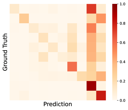
Figure 5: The normalized confusion matrix of ER and ER DDN based on Split CIFAR-10 with buffer size M=0.2K.

Table 5: Comparison for different methods of each task accuracy $a_{t,T}(t=1,2,...T)$ after the whole training based on Split CIFAR-10 with buffer size M=0.2K and M=0.5K.

	method	$a_{1,5}$	$a_{2,5}$	$a_{3,5}$	$a_{4,5}$	$a_{5,5}$	ACC$\uparrow$	FM$\downarrow$
	ER	18.42	18.64	23.38	36.36	83.44	36.05	49.99
	ER DDN	32.45	19.95	30.47	47.12	79.71	41.94	35.29
	DER++	31.27	26.12	28.63	44.27	77.42	41.54	39.50
	DER++ DDN	24.63	27.60	34.96	44.72	82.22	42.82	37.26
	CLSER	21.66	15.60	27.61	44.13	86.14	39.03	48.50
	CLSER DDN	27.50	19.11	31.68	45.83	80.68	40.96	40.07
	ER-ACE	48.93	33.20	38.52	53.41	40.02	42.81	17.33
M=0.2K	ER-ACE DDN	46.12	29.50	38.44	56.70	50.41	44.23	21.59
	ER	30.35	26.03	37.51	48.02	79.86	44.35	36.90
	ER DDN	40.25	34.51	39.54	49.03	77.25	48.11	32.30
	DER++	39.03	36.97	36.63	50.51	82.44	49.11	34.24
	DER++ DDN	40.70	36.26	38.23	54.43	77.82	49.48	28.19
	CLSER	34.10	27.13	32.63	47.99	81.09	44.58	37.31
	CLSER DDN	40.74	34.37	32.71	53.73	75.29	47.37	29.75
	ER-ACE	52.88	32.42	49.68	58.02	42.13	47.02	17.54
M=0.5K	ER-ACE DDN	52.31	34.20	43.28	62.11	54.68	49.31	16.84

C.3 Comparison methods

We provide a detailed induction of the four baselines and other comparison methods mentioned in the Table 1:

ER (Ratcliff, 1990a) is the most common replay-based continual learning method, which trains the new samples with the memory buffer samples together. Specifically, under the online CL setting, ER employs reservoir sampling to construct the memory buffer, which can be regarded as a balanced dataset to approximate the data distribution of all encountered tasks.

DER++ (Buzzega et al., 2020) builds upon ER by integrating an additional knowledge distillation, which calculates the MSE loss between the logits predicted by the current model and previous logits predicted by the old model. To reduce the memory size, DER++ directly stores previous logits with the memory buffer samples.

CLSER (Arani et al., 2022) incorporates a fast learning module for adapting to new tasks and a slow learning module for stabilizing old knowledge integration based on a complementary learning system (CLS). The collaboration between these two modules significantly reduce forgetting in CL.

ER-ACE(Caccia et al., 2021) shields old classes during updates and uses asymmetric update rules to encourage new classes to adapt to old ones. For the incoming new samples, ER-ACE masks the predicted probabilities corresponding to old classes, thereby preventing the gradients of new samples from negatively impacting the discriminative ability of the old classes.

iCarl (Rebuffi et al., 2017) proposes the nearest class mean (NCM) classification rule, selecting old training samples closest to the feature mean of each class for replay. It leverages knowledge distillation and prototype rehearsal for representation learning.

LUCIR (Hou et al., 2019) aims to balance the influence of new and old tasks. Specifically, ER-ACE employs cosine normalization to address the imbalance in embeddings between new and old classes. It further aligns embeddings provided by new and old models by minimizing their discrepancy. Additionally, it also maximizes the inter-class differences to enhance the model’s discriminative ability.

BIC (Wu et al., 2019) introduces an affine transformation to the classifier to correct the classification bias in the CL process. This method adopts a two-stage training approach. In the first stage, the classification model is trained by ER, while in the second stage, the affine transformation is trained by the memory buffer, which is an approximation of all data distributions.

LoDM (Yang et al., 2023) proposed a plugin module for previous dataset distillation methods. For example, based on DM (Zhao & Bilen, 2023), LoDM decomposed the synthetic images as two low-rank matrices to reduce the optimization parameters in image space, which significantly reduces the calculation in bi-level optimization. However, LoDM treats CL solely as a downstream application and performs distillation for each individual task, which easily neglects the global relationship between sequential tasks.

Mnemonics (Liu et al., 2020) optimized examples saved in the memory buffer for each task individually as we introduced in Eqn. (3). This formulation only distilled the intra-task information for the current task while ignoring the correlation between different tasks.

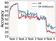
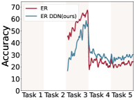
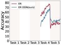
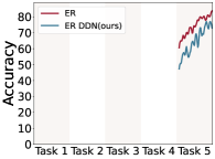
Figure 6: The accuracy of each task in the whole training process on Split CIFAR-10 with buffer size M=0.2K .

Appendix D Addational experiments

D.1 Confusion matrix

We visualized the confusion matrices of the baseline ER and our proposed ER DDN to better illustrate their performance in classifying samples from different classes. The horizontal axis of the confusion matrix represents the predicted classes, while the vertical axis represents the ground truth classes. Values along the diagonal indicate the number of correctly classified samples. As shown in the Fig. 5, Fig. 5 represents the confusion matrix for ER. It is evident that ER exhibits a strong bias towards predicting test samples as belonging to new classes. This bias leads to a higher misclassification rate for samples from old classes, exacerbating catastrophic forgetting. In contrast, due to the incorporation of soft-label distillation, ER DDN(ours) in Fig. 5, demonstrates superior retention of old-class information and effectively mitigates the bias towards new classes. During testing, predictions are more balanced between old and new classes, resulting in an overall improvement in classification performance.

D.2 Accuracy of each task

To comprehensively analyze how our method alleviates forgetting, we evaluated the accuracy of all tasks at the end of training, $i.e.$, $a_{t,T}(t=1,2,...T)$ to assess the model’s performance across different tasks. Under the online learning setting, we compared our method with various baselines on the Split CIFAR-10 dataset with buffer sizes of M=0.2K and M=0.5K.
The experimental results demonstrate that our method significantly improves the classification accuracy of old classes, particularly for ER with buffer sizes of M=0.2K and M=0.5K, the improvement in old-class accuracy is especially notable. This enhancement effectively mitigates the bias toward new classes, thereby improving overall performance. Further analysis reveals that the performance gains primarily stem from better accuracy on old classes. Specifically, when the buffer size is M=0.2K, our method reduces the forgetting measure (FM) by 14.7%, highlighting its strong capability in alleviating forgetting and preserving old-class information.

D.3 Analyse of each task accuracy

To investigate the accuracy trends of each task throughout the training process, Fig. 6 illustrates a comparison between the baseline ER and our proposed ER DDN on the Split CIFAR-10 dataset with buffer size M=0.2K. Each subplot represents the accuracy progression of task $i$ over the course of training. The results clearly show that our method consistently outperforms ER across the entire process. Notably, after a task transitions to being an old task, its accuracy during subsequent training remains significantly higher than that of ER. This indicates that our approach is more effective at retaining knowledge from old tasks, significantly mitigating catastrophic forgetting. These findings further validate the effectiveness of our method DDN in consolidating old task knowledge within the continual learning framework.

References

- Aljundi et al. (2019a) Aljundi, R., Belilovsky, E., Tuytelaars, T., Charlin, L., Caccia, M., Lin, M., and Page-Caccia, L. Online continual learning with maximal interfered retrieval. Advances in neural information processing systems, 32, 2019a.
- Aljundi et al. (2019b) Aljundi, R., Lin, M., Goujaud, B., and Bengio, Y. Gradient based sample selection for online continual learning. Advances in neural information processing systems, 32, 2019b.
- Arani et al. (2022) Arani, E., Sarfraz, F., and Zonooz, B. Learning fast, learning slow: A general continual learning method based on complementary learning system. arXiv preprint arXiv:2201.12604, 2022.
- Bang et al. (2021) Bang, J., Kim, H., Yoo, Y., Ha, J.-W., and Choi, J. Rainbow memory: Continual learning with a memory of diverse samples. In Proceedings of the IEEE/CVF conference on computer vision and pattern recognition, pp. 8218–8227, 2021.
- Borsos et al. (2020) Borsos, Z., Mutny, M., and Krause, A. Coresets via bilevel optimization for continual learning and streaming. Advances in neural information processing systems, 33:14879–14890, 2020.
- Buzzega et al. (2020) Buzzega, P., Boschini, M., Porrello, A., Abati, D., and Calderara, S. Dark experience for general continual learning: a strong, simple baseline. Advances in neural information processing systems, 33:15920–15930, 2020.
- Caccia et al. (2021) Caccia, L., Aljundi, R., Asadi, N., Tuytelaars, T., Pineau, J., and Belilovsky, E. New insights on reducing abrupt representation change in online continual learning. arXiv preprint arXiv:2104.05025, 2021.
- Cazenavette et al. (2022) Cazenavette, G., Wang, T., Torralba, A., Efros, A. A., and Zhu, J.-Y. Dataset distillation by matching training trajectories. In Proceedings of the IEEE/CVF Conference on Computer Vision and Pattern Recognition, pp. 4750–4759, 2022.
- Chaudhry et al. (2018a) Chaudhry, A., Dokania, P. K., Ajanthan, T., and Torr, P. H. Riemannian walk for incremental learning: Understanding forgetting and intransigence. In Proceedings of the European conference on computer vision (ECCV), pp. 532–547, 2018a.
- Chaudhry et al. (2018b) Chaudhry, A., Ranzato, M., Rohrbach, M., and Elhoseiny, M. Efficient lifelong learning with a-gem. In International Conference on Learning Representations (ICLR), 2018b.
- Cui et al. (2023) Cui, J., Wang, R., Si, S., and Hsieh, C.-J. Scaling up dataset distillation to imagenet-1k with constant memory. In International Conference on Machine Learning, pp. 6565–6590. PMLR, 2023.
- Finn et al. (2017) Finn, C., Abbeel, P., and Levine, S. Model-agnostic meta-learning for fast adaptation of deep networks. In International conference on machine learning, pp. 1126–1135. PMLR, 2017.
- Gal & Ghahramani (2016) Gal, Y. and Ghahramani, Z. Dropout as a bayesian approximation: Representing model uncertainty in deep learning. In international conference on machine learning, pp. 1050–1059. PMLR, 2016.
- Gretton et al. (2012) Gretton, A., Borgwardt, K. M., Rasch, M. J., Schölkopf, B., and Smola, A. A kernel two-sample test. The Journal of Machine Learning Research, 13(1):723–773, 2012.
- Hao et al. (2024) Hao, J., Ji, K., and Liu, M. Bilevel coreset selection in continual learning: A new formulation and algorithm. Advances in Neural Information Processing Systems, 36, 2024.
- Haykin (1998) Haykin, S. Neural networks: a comprehensive foundation. Prentice Hall PTR, 1998.
- Hou et al. (2019) Hou, S., Pan, X., Loy, C. C., Wang, Z., and Lin, D. Learning a unified classifier incrementally via rebalancing. In 2019 IEEE/CVF Conference on Computer Vision and Pattern Recognition (CVPR), pp. 831–839, 2019.
- Jiang et al. (2023) Jiang, Z., Gu, J., Liu, M., and Pan, D. Z. Delving into effective gradient matching for dataset condensation. In 2023 IEEE International Conference on Omni-layer Intelligent Systems (COINS), pp. 1–6. IEEE, 2023.
- Kim et al. (2022) Kim, J.-H., Kim, J., Oh, S. J., Yun, S., Song, H., Jeong, J., Ha, J.-W., and Song, H. O. Dataset condensation via efficient synthetic-data parameterization. In International Conference on Machine Learning, pp. 11102–11118. PMLR, 2022.
- Kingma & Ba (2014) Kingma, D. and Ba, J. Adam: A method for stochastic optimization. Computer Science, 2014.
- Kirkpatrick et al. (2017) Kirkpatrick, J., Pascanu, R., Rabinowitz, N., Veness, J., Desjardins, G., Rusu, A., et al. Overcoming catastrophic forgetting in neural networks. Proceedings of the National Academy of Sciences, 114(13):3521–3526, 2017.
- Krizhevsky et al. (2009) Krizhevsky, A., Hinton, G., et al. Learning multiple layers of features from tiny images. 2009.
- Lee et al. (2022) Lee, S., Chun, S., Jung, S., Yun, S., and Yoon, S. Dataset condensation with contrastive signals. In International Conference on Machine Learning, pp. 12352–12364. PMLR, 2022.
- Li et al. (2024) Li, G., Togo, R., Ogawa, T., and Haseyama, M. Dataset distillation using parameter pruning. IEICE Transactions on Fundamentals of Electronics, Communications and Computer Sciences, 107(6):936–940, 2024.
- Li & Hoiem (2018) Li, Z. and Hoiem, D. Learning without forgetting. IEEE Transactions on Pattern Analysis and Machine Intelligence, 40(12):2935–2947, 2018. doi: 10.1109/TPAMI.2017.2773081.
- Liu et al. (2020) Liu, Y., Su, Y., Liu, A.-A., Schiele, B., and Sun, Q. Mnemonics training: Multi-class incremental learning without forgetting. In Proceedings of the IEEE/CVF conference on Computer Vision and Pattern Recognition, pp. 12245–12254, 2020.
- Lopez-Paz & Ranzato (2017) Lopez-Paz, D. and Ranzato, M. Gradient episodic memory for continual learning. In Advances in Neural Information Processing Systems, volume 30. Neural Information Processing Systems (NeurIPS), 2017.
- McCloskey & Cohen (1989) McCloskey, M. and Cohen, N. J. Catastrophic interference in connectionist networks: The sequential learning problem. In Psychology of learning and motivation, volume 24, pp. 109–165. Elsevier, 1989.
- Piao et al. (2024) Piao, H., Wu, Y., Wu, D., and Wei, Y. Federated continual learning via prompt-based dual knowledge transfer. In Forty-first International Conference on Machine Learning, 2024.
- Pouransari & Ghili (2014) Pouransari, H. and Ghili, S. Tiny imagenet visual recognition challenge, 2014. 6.
- Ratcliff (1990a) Ratcliff, R. Connectionist models of recognition memory: constraints imposed by learning and forgetting functions. Psychological review, 97(2):285, 1990a.
- Ratcliff (1990b) Ratcliff, R. Connectionist models of recognition memory: constraints imposed by learning and forgetting functions. Psychological review, 97(2):285, 1990b.
- Rebuffi et al. (2017) Rebuffi, S.-A., Kolesnikov, A., Sperl, G., and Lampert, C. H. icarl: Incremental classifier and representation learning. In Proceedings of the IEEE conference on Computer Vision and Pattern Recognition, pp. 2001–2010, 2017.
- Rusu et al. (2017) Rusu, A. A., Rusu, I. A., Rao, D., Desjardins, G., He, B., Horgan, D., Ghemawat, S., Legenstein, R., Schmidhuber, J., et al. Learning to learn without forgetting by maximizing transfer and minimizing interference. In Proceedings of the 5th International Conference on Learning Representations (ICLR), 2017.
- Shim et al. (2021) Shim, D., Mai, Z., Jeong, J., Sanner, S., Kim, H., and Jang, J. Online class-incremental continual learning with adversarial shapley value. In Proceedings of the AAAI Conference on Artificial Intelligence, volume 35, pp. 9630–9638, 2021.
- Thrun & Mitchell (1995) Thrun, S. and Mitchell, T. M. Lifelong robot learning. Robotics and autonomous systems, 15(1-2):25–46, 1995.
- Tiwari et al. (2022) Tiwari, R., Killamsetty, K., Iyer, R., and Shenoy, P. Gcr: Gradient coreset based replay buffer selection for continual learning. In Proceedings of the IEEE/CVF Conference on Computer Vision and Pattern Recognition, pp. 99–108, 2022.
- Vitter (1985) Vitter, J. S. Random sampling with a reservoir. ACM Transactions on Mathematical Software (TOMS), 11(1):37–57, 1985.
- Wang et al. (2022a) Wang, K., Zhao, B., Peng, X., Zhu, Z., Yang, S., Wang, S., Huang, G., Bilen, H., Wang, X., and You, Y. Cafe: Learning to condense dataset by aligning features. In Proceedings of the IEEE/CVF Conference on Computer Vision and Pattern Recognition, pp. 12196–12205, 2022a.
- Wang et al. (2023) Wang, Q., Wang, R., Wu, Y., Jia, X., and Meng, D. Cba: Improving online continual learning via continual bias adaptor. In Proceedings of the IEEE/CVF International Conference on Computer Vision, pp. 19082–19092, 2023.
- Wang et al. (2024) Wang, Q., Wang, R., Wu, Y., Jia, X., Zhou, M., and Meng, D. Dual-cba: Improving online continual learning via dual continual bias adaptors from a bi-level optimization perspective. arXiv preprint arXiv:2408.13991, 2024.
- Wang et al. (2018) Wang, T., Zhu, J.-Y., Torralba, A., and Efros, A. A. Dataset distillation. arXiv preprint arXiv:1811.10959, 2018.
- Wang et al. (2022b) Wang, Z., Shen, L., Fang, L., Suo, Q., Duan, T., and Gao, M. Improving task-free continual learning by distributionally robust memory evolution. In International conference on machine learning, pp. 22985–22998. PMLR, 2022b.
- Wang et al. (2025) Wang, Z., Wu, Y., Wang, R., Lin, H., Wang, Q., Zhao, Q., and Meng, D. Singular value fine-tuning for few-shot class-incremental learning. arXiv preprint arXiv:2503.10214, 2025.
- Wu et al. (2019) Wu, Y., Chen, Y., Wang, L., Ye, Y., Liu, Z., Guo, Y., and Fu, Y. Large scale incremental learning. In 2019 IEEE/CVF Conference on Computer Vision and Pattern Recognition (CVPR), pp. 374–382, 2019. doi: 10.1109/CVPR.2019.00046.
- Wu et al. (2024a) Wu, Y., Huang, L.-K., Wang, R., Meng, D., and Wei, Y. Meta continual learning revisited: Implicitly enhancing online hessian approximation via variance reduction. In The Twelfth International Conference on Learning Representations, 2024a.
- Wu et al. (2024b) Wu, Y., Wang, H., Zhao, P., Zheng, Y., Wei, Y., and Huang, L.-K. Mitigating catastrophic forgetting in online continual learning by modeling previous task interrelations via pareto optimization. In Forty-first International Conference on Machine Learning, 2024b.
- Wu et al. (2025) Wu, Y., Piao, H., Huang, L.-K., Wang, R., Li, W., Pfister, H., Meng, D., Ma, K., and Wei, Y. SD-LoRA: Scalable Decoupled Low-Rank Adaptation for Class Incremental Learning. The Thirteenth International Conference on Learning Representations, 2025.
- Yang et al. (2023) Yang, E., Shen, L., Wang, Z., Liu, T., and Guo, G. An efficient dataset condensation plugin and its application to continual learning. Advances in Neural Information Processing Systems, 36, 2023.
- Yang et al. (2024) Yang, J., Wu, Y., Cen, J., Huang, W., Wang, H., and Zhang, J. Continual learning for segment anything model adaptation. arXiv preprint arXiv:2412.06418, 2024.
- Yoon et al. (2021) Yoon, J., Madaan, D., Yang, E., and Hwang, S. J. Online coreset selection for rehearsal-based continual learning. arXiv preprint arXiv:2106.01085, 2021.
- Yuan et al. (2020) Yuan, L., Tay, F. E., Li, G., Wang, T., and Feng, J. Revisiting knowledge distillation via label smoothing regularization. In 2020 IEEE/CVF Conference on Computer Vision and Pattern Recognition (CVPR), pp. 3902–3910, 2020. doi: 10.1109/CVPR42600.2020.00396.
- Zhang et al. (2023) Zhang, L., Zhang, J., Lei, B., Mukherjee, S., Pan, X., Zhao, B., Ding, C., Li, Y., and Xu, D. Accelerating dataset distillation via model augmentation. In Proceedings of the IEEE/CVF Conference on Computer Vision and Pattern Recognition, pp. 11950–11959, 2023.
- Zhao & Bilen (2021) Zhao, B. and Bilen, H. Dataset condensation with differentiable siamese augmentation. In International Conference on Machine Learning, pp. 12674–12685. PMLR, 2021.
- Zhao & Bilen (2023) Zhao, B. and Bilen, H. Dataset condensation with distribution matching. In Proceedings of the IEEE/CVF Winter Conference on Applications of Computer Vision, pp. 6514–6523, 2023.
- Zhao et al. (2020) Zhao, B., Mopuri, K. R., and Bilen, H. Dataset condensation with gradient matching. arXiv preprint arXiv:2006.05929, 2020.
- Zhiqi et al. (2025) Zhiqi, K., Wang, L., Zhang, X., and Alahari, K. Advancing prompt-based methods for replay-independent general continual learning. In The Thirteenth International Conference on Learning Representations, 2025.
- Zhou et al. (2022) Zhou, X., Pi, R., Zhang, W., Lin, Y., Chen, Z., and Zhang, T. Probabilistic bilevel coreset selection. In International Conference on Machine Learning, pp. 27287–27302. PMLR, 2022.