Graph Wave Networks
Abstract.
Dynamics modeling has been introduced as a novel paradigm in message passing (MP) of graph neural networks (GNNs). Existing methods consider MP between nodes as a heat diffusion process, and leverage heat equation to model the temporal evolution of nodes in the embedding space. However, heat equation can hardly depict the wave nature of graph signals in graph signal processing. Besides, heat equation is essentially a partial differential equation (PDE) involving a first partial derivative of time, whose numerical solution usually has low stability, and leads to inefficient model training. In this paper, we would like to depict more wave details in MP, since graph signals are essentially wave signals that can be seen as a superposition of a series of waves in the form of eigenvector. This motivates us to consider MP as a wave propagation process to capture the temporal evolution of wave signals in the space. Based on wave equation in physics, we innovatively develop a graph wave equation to leverage the wave propagation on graphs. In details, we demonstrate that the graph wave equation can be connected to traditional spectral GNNs, facilitating the design of graph wave networks (GWNs) based on various Laplacians and enhancing the performance of the spectral GNNs. Besides, the graph wave equation is particularly a PDE involving a second partial derivative of time, which has stronger stability on graphs than the heat equation that involves a first partial derivative of time. Additionally, we theoretically prove that the numerical solution derived from the graph wave equation are constantly stable, enabling to significantly enhance model efficiency while ensuring its performance. Extensive experiments show that GWNs achieve state-of-the-art and efficient performance on benchmark datasets, and exhibit outstanding performance in addressing challenging graph problems, such as over-smoothing and heterophily. Our code is available at https://github.com/YueAWu/Graph-Wave-Networks.
1. Introduction
The widespread availability of graph data has propelled the development of graph neural networks (GNNs) (Wu et al., 2021). These methods have achieved significant success in various applications, such as recommender systems (Wu et al., 2023), social network analysis (Lin et al., 2021), particle physics (Shlomi et al., 2021), and drug discovery (Gaudelet et al., 2021).
Currently, mainstream GNNs (Defferrard et al., 2016; Kipf and Welling, 2017) develop message passing (MP) paradigm with graph signal processing (Shuman et al., 2013), which delivers messages node-by-node by stacking graph convolutional layers. In fact, the MP paradigm can be modelled as a differential equation (Chamberlain et al., 2021). Recent studies explore partial differential equations (PDEs) (Chamberlain et al., 2021; Thorpe et al., 2022; Li et al., 2024) to consider the spatial and temporal relationships in MP. Intuitively, they analogize MP to a heat diffusion process between nodes, and thus leverage the heat equation to model nodes in the embedding space. In physics, the heat equation describes the evolution of temperature in the space over time. Consider 3-dimension spatial variables in the space and a time variable , the Heat Equation is:
| (1) |
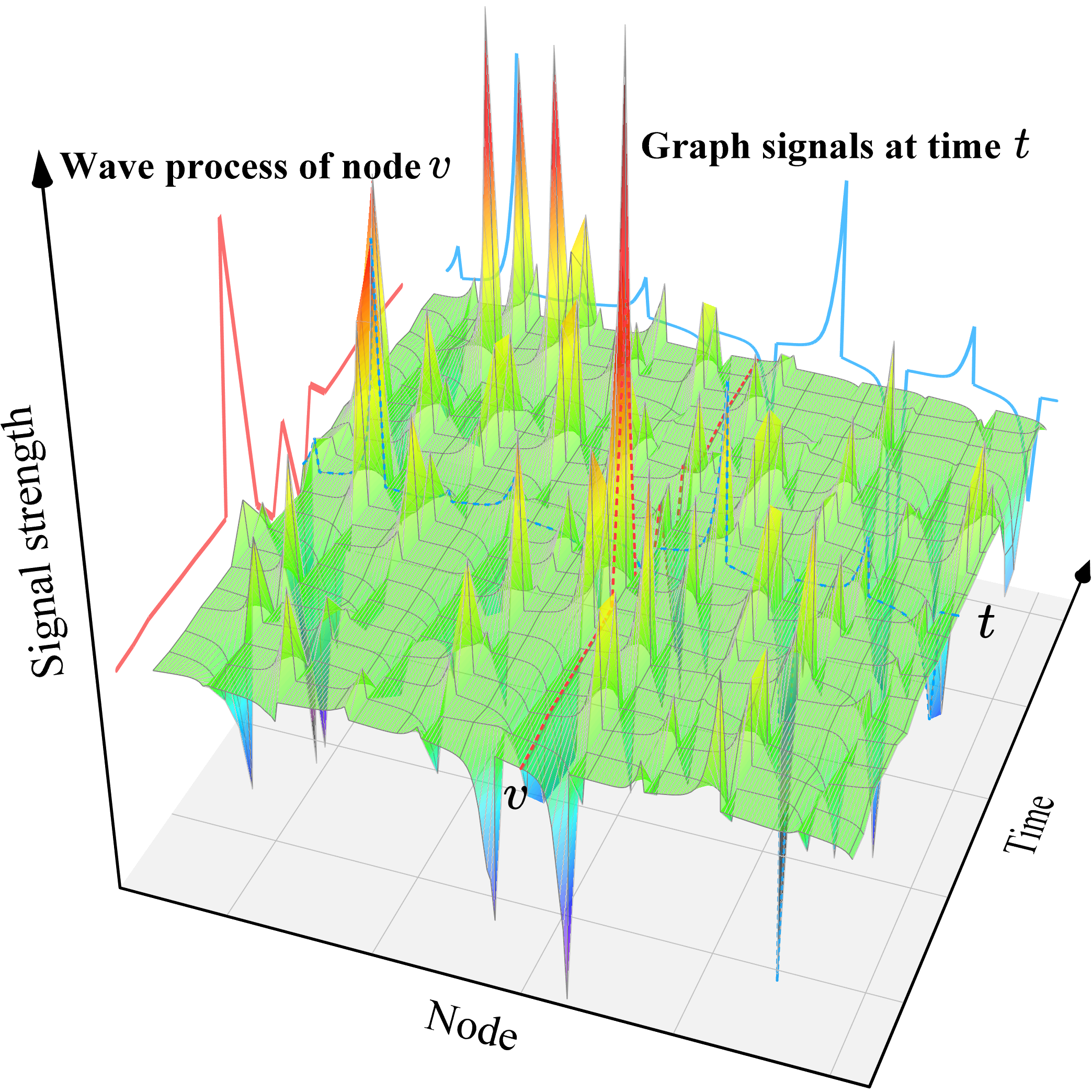
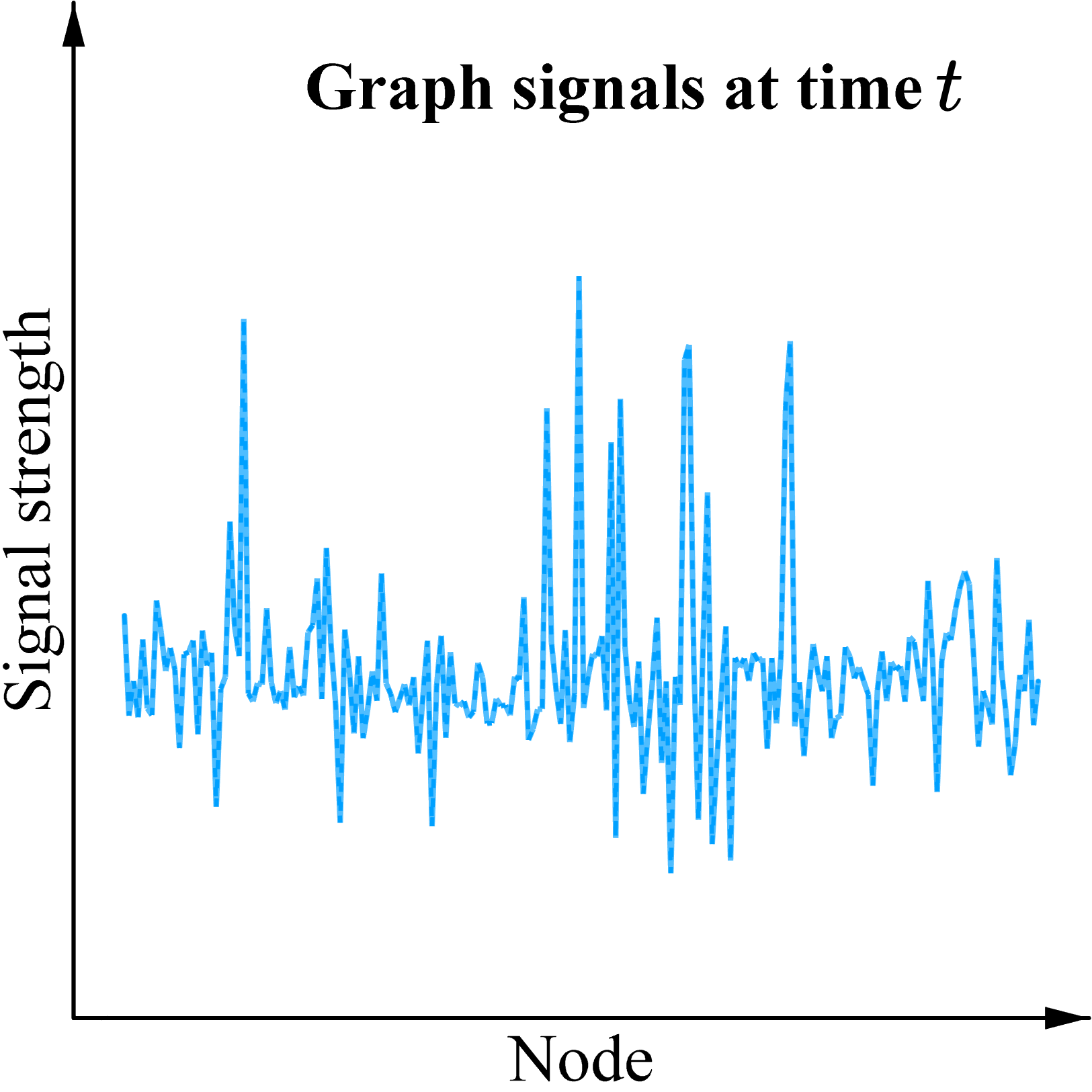
where is the abbreviation symbol for , denoting the temperature at position and time , and is a coefficient called the thermal diffusivity of the medium. However, in context of graph learning, these methods suffer from two drawbacks: First, the heat equation can hardly depict the wave nature of graph signals. In graph signal processing theory (Shuman et al., 2013), the graph can be seen as a combination of waves with different frequencies, where we show the graph wave spectrum in Figure 1 (Top). The heat equation is naturally not capable to process the details of wave property in message passing, which leads to coarse and sub-optimal GNN designs. Second, the heat equation is essentially a PDE involving a first partial derivative of time, yet its stability of numerical solution can be poor on graph. This requires small time step lengths in solving PDE, leading to low efficiency in model training, and can be easily affected by initial values and generate unsatisfactory performance. We also give the experimental evidence in Sec. 4.
Unlike previous studies (Chamberlain et al., 2021; Thorpe et al., 2022; Li et al., 2024) that regard MP as a heat diffusion process, we innovatively analogize MP to a wave propagation process. Particularly, MP basically embodies the information propagation along the nodes at different spatial positions and temporal steps, which bears a strong resemblance to the propagation of waves in physics, such as electromagnetic waves. To depict the wave propagation process, we explore the wave equation, a PDE involving the second derivative of time, which describes the evolution of wave intensity over time and has wide applicability in physics. Also consider the three spatial variables and a time variable , the Wave Equation is:
| (2) |
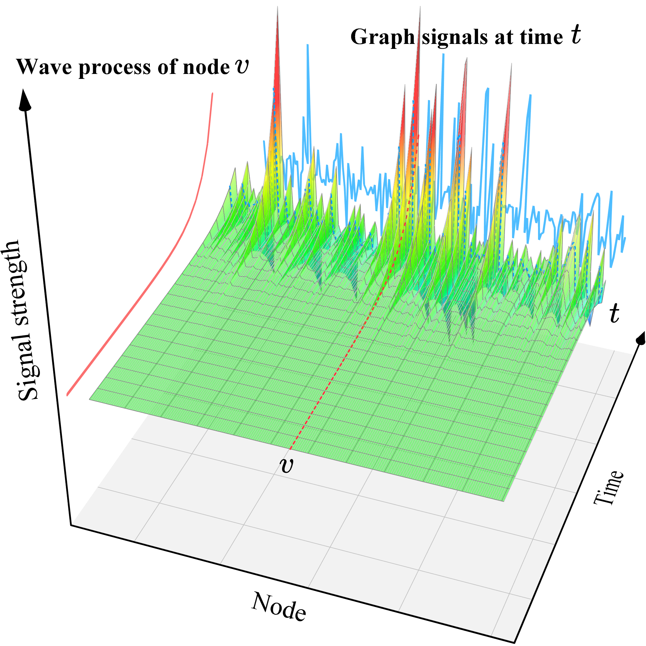
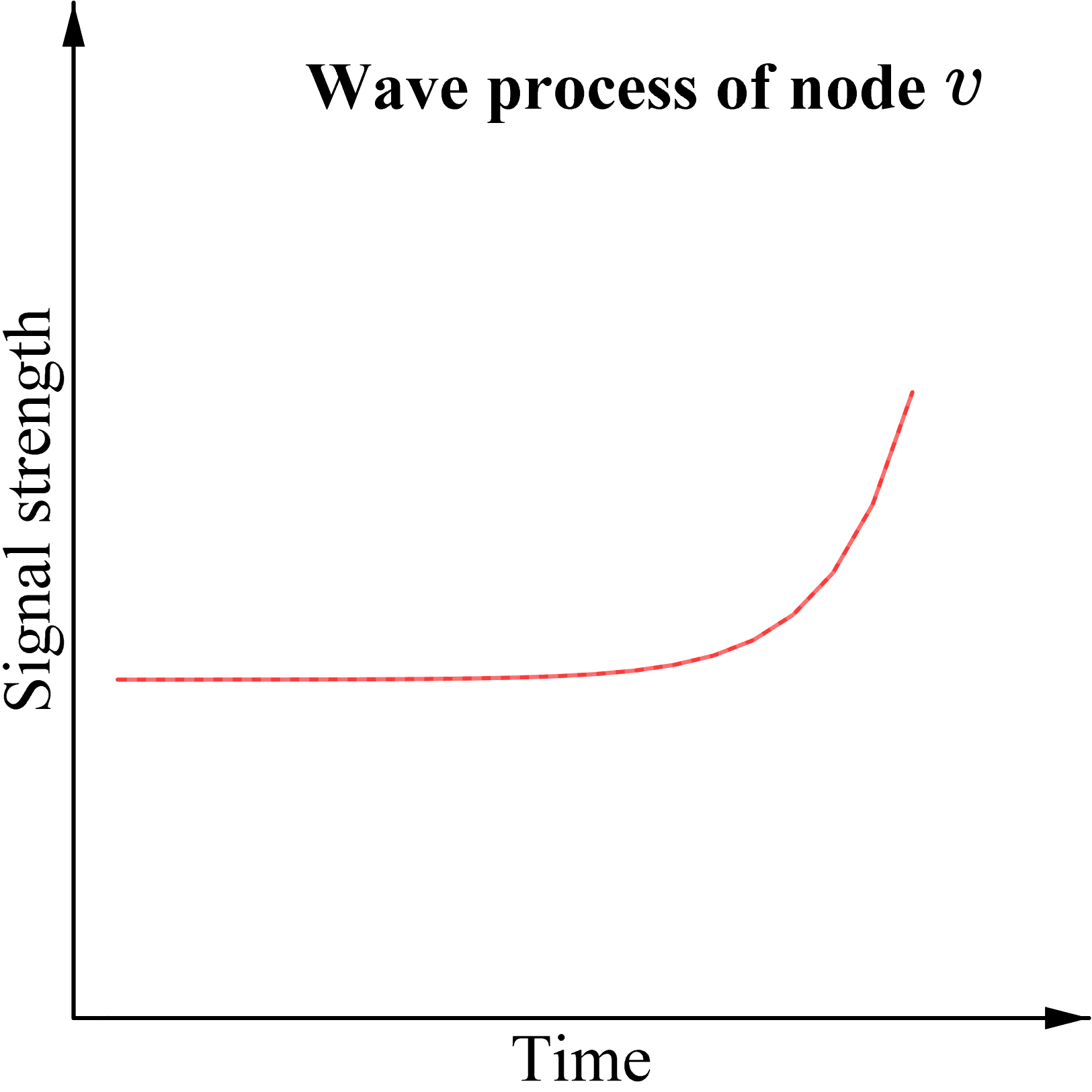
where is the abbreviation symbol for , denoting the wave intensity at position and time , and is a coefficient denoting the propagation speed of the wave. Notably, though the wave equation has similar formulation as heat equation, it has intrinsically different properties in the context of graph learning: First, wave equation is naturally suitable for MP in GNNs. Since GNN is actually a wave filter of frequencies, it can be achieved by Laplacian. It investigates more details in processcing graph signals, offering higher accuracy and practicality compared to heat equation. Second, the wave equation is essentially a PDE involving a second partial derivative of time, which can offer stronger stable condition on graph. This property provides more efficient training process that allows larger time step lengths, and often generates robust experimental results (see Figure 4). The wave propagation process on graph can be depicted as Figure 1 (Bottom).
![[Uncaptioned image]](/html/2505.20034/assets/x2.png)
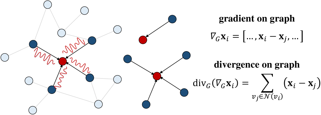
Though applying the above wave equation to MP is attractive and reasonable, the specific MP formulation of wave equation is not obvious, and it is non-trivial to conduct further exploration. To this end, our breakthrough point is to formulate the MP process with the wave equation at each node, since once the MP process is specified, the overall GNN is designed. Therefore, we first would like to derive graph wave equation for MP. Inspired by Chamberlain et al. (2021), we let the gradient on graph be the difference of features between a central node and each of its neighbors, and the divergence be the total difference of them. Thereby we can derive the formulation in graph wave equation, and the details are shown in Table 1. By introducing the characteristics of graph Laplacian, the graph wave equation can be further rewritten into a brief form for the solution of PDEs (detailed in Sec. 3.2).
Based upon the above derived graph wave equation, we then would like to achieve the MP for GNN design by solving PDEs. In fact, the solution of PDEs is often an iterative node feature update process, which can actually be interpreted as the MP process. Existing PDE-based GNN methods (Nguyen et al., 2024; Chamberlain et al., 2021) utilizing the forward Euler method to solve PDEs, resulting in conditionally stable explicit schemes, making it difficult to balance the performance and efficiency of the model. Besides, Chamberlain et al. (2021) also attempt implicit schemes through the backward Euler method, which are constantly stable but require solving linear systems, leading to higher computational complexity and lower efficiency compared to the explicit schemes. In this paper, we use the forward Euler method to solve the graph wave equation, which can obtain constantly stable explicit schemes. This allows the model to significantly improve convergence rates by selecting larger time step lengths, thereby enhancing efficiency of operation while guaranteeing model performance (detailed in Sec. 3.3). Based upon the above designs, we propose the Graph Wave Networks (termed as GWN) with MP formulated by graph wave equation. Two specified implementations are provided to achieve our GWN according to different specification of Laplacians (detailed in Sec. 3.4).
Our main contributions can be summarized as follows:
-
•
For the first time, we model the message passing from an innovative perspective of a wave propagation process, thereby maintaining the wave nature in graph convolutional operation.
-
•
We develop wave equation into graph wave equation, and propose a novel graph wave network, namely GWN. It establishes a connection between wave equation and traditional spectral GNNs, enhancing them with more details of waves on graphs.
-
•
Through the theoretical evidence, we prove that the explicit scheme of the graph wave equation is constantly stable, allowing significant efficiency improvements while guaranteeing robust model prediction results.
-
•
We conduct extensive experiments on 9 benchmark datasets. Experimental results substantiate that GWN outperforms previous state-of-the-art methods and achieves efficient performance in alleviating over-smoothing and heterophily.
2. Preliminaries
In this section, we discuss graph signal processing in traditional GNNs, and then introduce fundamental concepts of wave equations.
2.1. Graph Signal Processing
Graph signal processing (Shuman et al., 2013) is a field that focuses on signal analysis and processing conducted on graphs.
Notations of Graph. Given a simple undirected graph , composed of a set of nodes and a set of edges , with nodes in total. Graph is associated with a feature matrix , where the -th row of corresponds to the feature vector of node , and the -th column of corresponds to the graph signal of dimension . We denote the adjacency matrix as and the degree matrix as with .
Spectral Graph Convolution. Traditional spectral GNNs design spectral graph convolution using the symmetric normalized Laplacian , which can be decomposed into , where is a diagonal matrix of eigenvalues and is a matrix of corresponding eigenvectors. Here, the eigenvalues satisfy . Based on this, the definition of spectral graph convolution is as follows:
| (3) |
where denotes the graph filter function.
2.2. Wave Equation
The wave equation describes the laws of waves in the space evolving over time, which has been widely adopted to analyze the characteristics of waves like electromagnetic waves in physics.
Given that is a scalar-valued function on that reflects the wave intensity, where denotes the spatial dimension, and denotes the time dimension, the wave equation can be formulated by the following partial differential equation (PDE):
| (4) |
where denotes Laplacian operator in mathematics, and denote gradient and divergence, respectively. denotes the propagation velocity of waves in the medium (such as the propagation velocity of electromagnetic waves in vacuum), which is a scalar or a function to describe the wave.
3. Wave Equation on Graphs
In this section, we would like to analyze the wave nature of graph signals, and propose graph wave equation with solutions for MP.
3.1. Graph and Wave
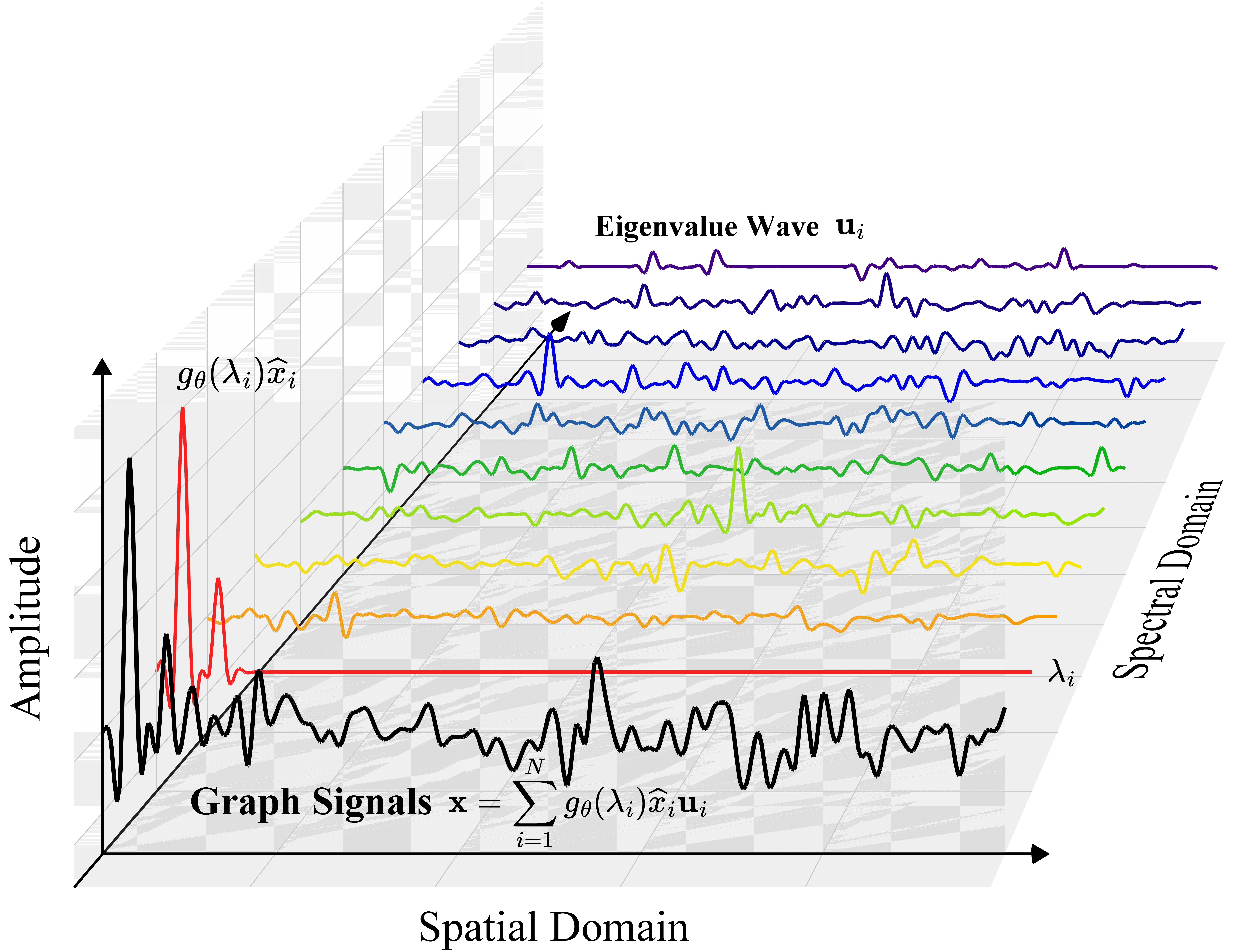
This section illustrates the connection between graphs and waves from the perspective of graph signal processing. For convenience, we use a toy example of graph signals with nodes embedded in -dimensional space , where the same principle can be extended to -dimensional space . First, the typical implementation of spectral graph convolution transforms graph signals by Fourier transform:
| (5) |
where the -th element of denotes the signal strength of the spectral signal corresponding to the eigenvalue in the spectral domain. Then, based upon them, the spectral graph convolution is defined as:
| (6) |
Finally, the inverse Fourier transform is used to map the spectral signal back to the spatial domain:
| (7) | ||||
Remark 1. The connection between graph and wave. From Eq. (7), we can observe that the graph signal in spatial domain can be treated as a linear combination of different eigenvalues in spectral domain, vividly depicted in Figure 1 (Top). Intuitively, we can interpret the eigenvalue as the frequency, its corresponding eigenvector as a particular type of wave, and denotes the amplitude of the wave. This reflects the wave nature of the spectral graph convolution on any given graphs.
3.2. Graph Wave Equation
We are going to extend the wave equation on the graph. Given the graph signal (, node features), for any node , its node representation acquires messages from its neighbors in GNNs. Then, we can derive the gradient of in MP on its graph by vector subtraction between and its neighbors, which actually captures their signal differences (Chamberlain et al., 2021):
| (8) |
where the gradient direction reflects the direction from to in MP, and the gradient magnitude measures the feature difference amount between and . Subsequently, we can derive the divergence of on by the sum of feature differences between the node and all its neighbor :
| (9) |
where the divergence actually measures the total difference between a node and its neighborhood. Finally, by substituting Eq. (9) into (4), we propose Graph Wave Equation on the graph:
| (10) |
where is the signal intensity (of all nodes) in the entire graph , and can be regarded as the node representations. Each row of involves a wave equation at a specific node. By introducing the form of Laplacian, we can rewrite Eq. (10) as follows (see Appendix A.1 for mathematical proof):
Proposition 1. Let denote the discrete form of the Laplacian operator . The graph wave equation can be rewritten as:
| (11) |
where we incorporate into for a simple form, , . Here, the propagation velocity controls the speed of wave propagation between nodes on the graph. Note that the propagation velocity can alternatively be constant or learnable parameters in practice, leading to different forms of Laplacian (detailed in Eq. (15) and (17) later). Benefit by treating as learnable parameters, we can redefine Laplacian with flexibility and establish a connection between wave equation and Laplacian-based spectral GNNs.
Remark 2. The connection between graph wave equation and spectral GNNs. With Eq. (11), we can easily combine the wave equation with spectral GNNs into graph wave equations. Thereby, the graph wave equation can be flexibly extended and achieved by specific designed Laplacians of existing spectral GNNs.
3.3. Solution of Graph Wave Equation
In general, it is often intractable to obtain an analytical solution for a PDE. Fortunately, there are numerical methods that can approximate PDE solutions. First, the continuous PDE can be discretized into a finite form of a linear algebraic system using the finite difference method. Then, an iteration process with initial values can be employed to solve this linear algebraic system. In the context of graphs, only the time dimension needs to be further discretized on each node. To this end, we employ a commonly-used discretization method in mathematics, namely forward Euler method, to solve the graph wave equation for node representations (i.e., ) (Chamberlain et al., 2021).
Formally, the forward Euler method discretizes the graph wave equation by performing forward difference in the time dimension, and then derives the explicit scheme:
| (12) |
where is the time step length. The initial values of and in the PDE can be obtained using the second-order central quotient:
| (13) |
where and can be practically achieved by neural networks, such as feedforward networks. Finally, the explicit scheme of the graph wave equation is given by:
| (14) |
Please see Appendix A.2 for the detailed derivation of the forward Euler method. In particular, we can interpret the above equation from the perspective of message passing:
Remark 3. The perspective of message passing. By decomposing into , the graph signal at time consists of two components: 1) the aggregation of neighbor information at time , and 2) the difference between the graph signal at times and .
3.4. Graph Wave Networks
In this section, we propose two specifications of GWNs with time-independent and time-dependent Laplacian, respectively.
Symmetric Normalized Laplacian.
We consider time-independent Laplacian, where we let the velocity be a constant. Typically, we adopt GCN (Kipf and Welling, 2017) as the base model and design a symmetric normalized Laplacian without self-loops, which behaves as a low-pass filter in the spectral domain:
| (15) |
GWN-sym. We propose the Graph Wave Network based on the symmetric normalized Laplacian. With the initial values given by Eq. (13), the feature matrix at time can be determined as:
| (16) |
The final feature matrix at the terminal time is transformed into a prediction matrix by an MLP as .
Frequency Adaptive Laplacian.
Next, we consider time-dependent Laplacian, where the velocity is non-constant learnable parameters. Typically, we adopt FAGCN (Bo et al., 2021) as the base model and propose a frequency adaptive Laplacian with a time-dependent learnable parameter , which designs both a low-pass filter and a high-pass filter in the spectral domain:
| (17) |
GWN-fa. We propose the Graph Wave Network based on the frequency adaptive Laplacian. The initial values are also given by Eq. (13), and the feature matrix at time can be determined as (see Appendix A.4 for detailed derivation):
| (18) |
where the element of is the attention weight between nodes and at time , and is a learnable parameter vector. Notably, when , the two nodes are more similar and GWN-fa behaves a low-pass filter; and when , two nodes are more dissimilar and GWN-fa behaves a high-pass filter. The final feature matrix at terminal time is also transformed into a prediction matrix by an MLP.
3.5. Stability
Stability is an important property of differential equations, which is closely related to the robustness in machine learning (Chamberlain et al., 2021), and refers to the property that small perturbations in initial values would not result in a significant change in solutions. We discuss the initial value stability of the explicit scheme . Formally, if there exists and a constant such that the inequality holds for all and , then the explicit scheme is said to be initial value stable. It is crucial to prove the stability of explicit schemes to ensure that the resulting GNNs is reliable and feasible. A commonly used method for proving stability is the matrix method:
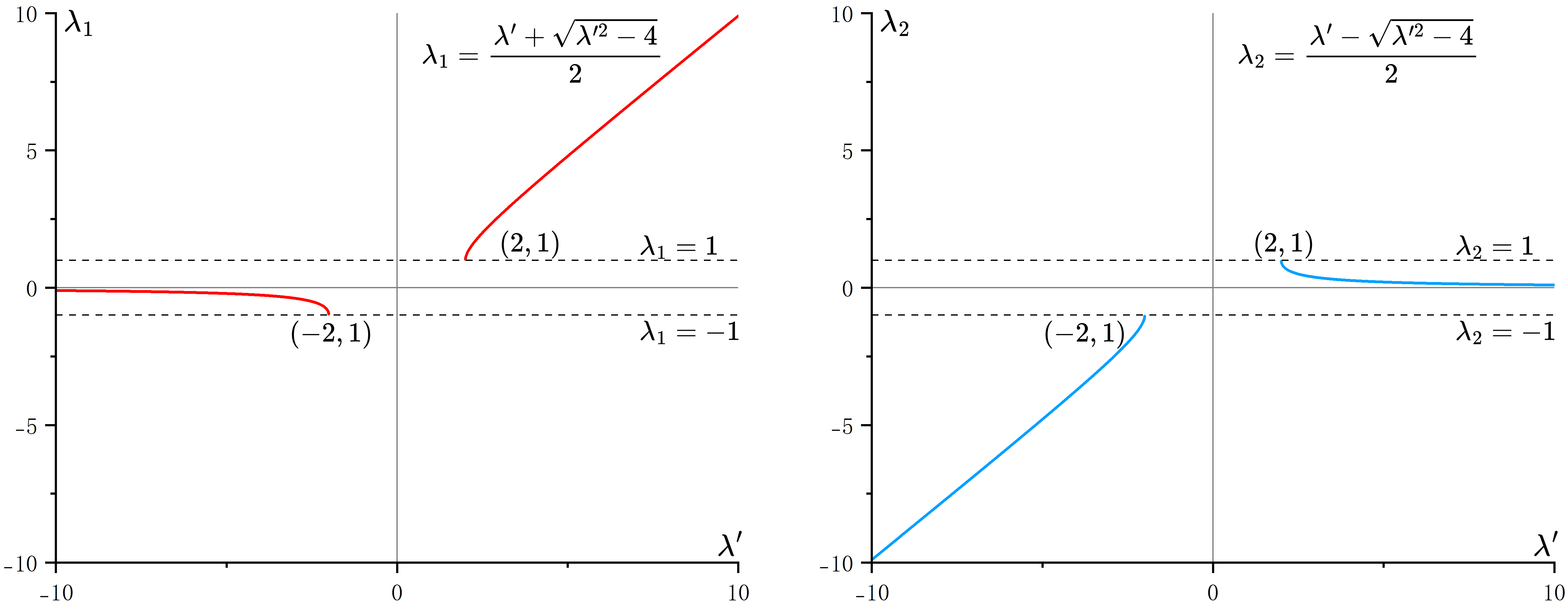
Theorem 1. Let denote the spectral radius of matrix , if , the numerical scheme is stable.
Based on Theorem 1, we prove that both the explicit schemes based on the symmetric normalized Laplacian (see Appendix A.3 for proof) and the frequency adaptive Laplacian (see Appendix A.5 for proof) are constantly stable.
Theorem 2. Given with , the explicit scheme is constantly stable for any .
Theorem 3. Given with , the explicit scheme is constantly stable for any .
Remark 4. The impact of constantly stability for models. Theoretically, we prove that the explicit scheme of the graph wave equation is constantly stable, guaranteeing the model performance would not be affected by the time step length, thus allowing to improve the efficiency by choosing a relatively larger .
Comparison with heat equation based GRAND
The explicit scheme of GRAND is , where is an attention matrix constrained to be a right stochastic matrix satisfying and . Benefiting from being a right stochastic matrix, the explicit scheme is stable and can be directly proven. However, it has the two deficiencies: First, the stability of explicit schemes is conditional (), striking a balance between performance and efficiency. Detailed comparisons and validations can be found in Sec. 4.4. Second, the attention scores are constrained to , which performs poorly in distinguishing inter-class nodes. In contrast, our GWN-fa acts as low-pass and high-pass filters when and respectively, enabling better handling of various types of graph.
3.6. Complexity Analysis
The number of learnable parameters of GWN-sym and GWN-fa are and , compared to in GRAND (Chamberlain et al., 2021). Here, , and denote the input dimension, the hidden layer dimension, and the number of classes, respectively. In general, . The computational complexity of each layer of GWN-sym and GWN-fa are and , compared to in GRAND. Here, , and are the number of nodes, edges and rewritten edges.
4. Experiments
| Datesets | Cora | CiteSeer | PubMed | Computers | Photo | CS | obgn-arxiv |
| GCN | 87.51 1.38 | 80.59 1.12 | 87.95 0.83 | 86.09 0.61 | 93.04 0.53 | 95.14 0.25 | 72.17 ± 0.33 |
| GAT | 87.42 1.46 | 80.16 1.63 | 85.91 1.26 | 87.89 0.82 | 93.53 0.58 | 94.37 0.28 | 73.65 0.11 |
| GraphSAGE | 87.50 1.45 | 79.39 1.38 | 89.64 0.73 | 88.53 0.70 | 94.49 0.55 | 95.93 0.25 | 71.39 ± 0.16 |
| GDC | 86.89 1.28 | 80.05 0.60 | 86.18 0.42 | 88.56 0.38 | 93.56 0.33 | 94.82 0.22 | |
| CGNN | 88.29 1.11 | 79.93 1.04 | 89.46 0.52 | 88.31 0.65 | 94.35 0.56 | 96.21 0.32 | 58.70 ± 2.50 |
| ADC∗ | 87.45 0.89 | 79.43 0.96 | 90.23 0.39 | 88.62 0.56 | 95.33 0.27 | 95.82 0.15 | |
| GADC | 87.64 0.64 | 78.62 0.57 | 88.58 0.48 | 87.78 0.54 | 94.70 0.35 | 96.16 0.29 | |
| GRAND∗ | 88.70 0.99 | 81.56 1.28 | 88.39 0.32 | 89.37 0.41 | 95.79 0.59 | 95.77 0.28 | 72.23 0.20 |
| GraphCON∗ | 87.81 0.92 | 79.68 1.23 | 88.54 1.32 | ||||
| GWN-sym | 89.61 0.87 | 81.81 1.70 | 90.56 0.54 | 90.10 0.87 | 95.31 0.65 | 96.66 0.26 | 72.19 0.20 |
| GWN-fa | 89.66 1.29 | 80.89 1.51 | 90.64 0.73 | 90.62 0.61 | 95.61 0.53 | 96.67 0.26 | 72.40 0.10 |
| Datesets | Actor | Texas | Cornell | Wisconsin | DeezerEurope | |||
| Splits | 60/20/20(%)† | 48/32/20(%)† | 60/20/20(%)‡ | 48/32/20(%)† | 60/20/20(%)‡ | 48/32/20(%)† | 60/20/20(%)‡ | 60/20/20(%)† |
| GCN | 27.32 1.10 | 55.14 5.16 | 79.33 4.47 | 60.54 5.30 | 69.53 11.79 | 51.76 3.06 | 63.94 4.93 | 62.23 0.53 |
| GAT | 27.44 0.89 | 52.16 6.63 | 79.59 9.21 | 61.89 5.05 | 66.91 15.99 | 49.41 4.09 | 63.45 11.65 | 61.09 0.77 |
| GraphSAGE | 34.23 0.99 | 82.43 6.14 | 86.02 4.78 | 75.95 5.01 | 85.06 5.12 | 81.18 5.56 | 89.56 3.99 | |
| MixHop | 32.22 2.34 | 77.84 7.73 | 73.51 6.34 | 75.88 4.90 | 66.80 0.58 | |||
| Geom-GCN | 31.59 1.15 | 66.76 2.72 | 60.54 3.67 | 64.51 3.66 | ||||
| H2GCN | 35.70 1.00 | 84.86 7.23 | 85.90 3.53 | 82.70 5.28 | 86.23 4.71 | 87.65 4.98 | 87.50 1.77 | 67.22 0.90 |
| LINKX | 36.10 1.55 | 74.60 8.37 | 77.84 5.81 | 75.49 5.72 | ||||
| WRGAT | 36.53 0.77 | 83.62 5.50 | 81.62 3.90 | 86.98 3.78 | ||||
| FAGCN | 34.82 1.35 | 82.43 6.89 | 85.57 4.75 | 79.19 9.79 | 86.38 5.33 | 82.94 7.95 | 84.88 9.19 | 66.86 0.53 |
| GPR-GNN | 35.16 0.90 | 78.38 4.36 | 91.89 4.08 | 80.27 8.11 | 85.91 4.60 | 82.94 4.21 | 93.84 3.16 | 66.90 0.50 |
| GGCN | 37.54 1.56 | 84.86 4.55 | 92.13 3.05 | 85.68 6.63 | 88.70 4.97 | 86.86 3.29 | 94.56 3.26 | |
| NLMLP | 85.40 3.80 | 84.90 5.70 | 87.30 4.30 | |||||
| GloGNN∗ | 37.70 1.40 | 84.05 4.90 | 85.95 5.10 | 88.04 3.22 | ||||
| NSD∗ | 37.81 1.15 | 85.95 5.51 | 84.86 4.71 | 89.41 4.74 | ||||
| ACM-GCN∗ | 37.31 1.09 | 88.38 3.43 | 86.49 6.73 | 88.43 3.66 | 67.50 0.53 | |||
| Ordered GNN | 37.99 1.70 | 86.22 4.12 | 90.82 4.18 | 87.03 4.73 | 88.09 3.36 | 88.04 3.63 | 93.62 2.91 | |
| GWN-sym | 39.97 1.72 | 89.85 5.05 | 91.64 3.74 | 88.11 3.17 | 89.57 3.54 | 90.88 4.43 | 93.38 3.18 | 68.15 0.77 |
| GWN-fa | 42.03 1.59 | 92.94 4.45 | 93.28 3.14 | 90.81 4.63 | 92.13 3.76 | 94.26 1.76 | 95.63 1.59 | 68.63 0.29 |
4.1. Experimental Setup
Datasets. Following the practices (Chamberlain et al., 2021; Rusch et al., 2022), we conduct node classification (Shchur et al., 2018) on the following real-world datasets (see Appendix B.1 for statistics): (1) homophilic datasets (Shchur et al., 2018; Yang et al., 2016): citation networks Cora, CiteSeer and PubMed, Amazon co-purchase networks Computers and Photo, and co-author networks CS; (2) heterophilic datasets (Rozemberczki et al., 2019; Pei et al., 2020; Rozemberczki and Sarkar, 2020a, b): co-occurrence graph Actor, WebKB datasets Texas, Cornell and Wisconsin, and social network DeezerEurope; (3) large-scale dataset (Hu et al., 2020): citation network ogbn-arxiv.
Baselines. We categorize all baselines into the following two classes: (1) mainstream GNNs: GCN (Kipf and Welling, 2017), GAT (Velickovic et al., 2018), GraphSAGE (Hamilton et al., 2017), SGC (Wu et al., 2019), JK-Net (Xu et al., 2018), ResGCN (Li et al., 2019), GCNII (Chen et al., 2020), FAGCN (Bo et al., 2021), GPR-GNN (Chien et al., 2021), AIR (Zhang et al., 2022), MixHop (Abu-El-Haija et al., 2019), Geom-GCN (Pei et al., 2020), H2GCN (Zhu et al., 2020), LINKX (Lim et al., 2021), WRGAT (Suresh et al., 2021), GGCN (Yan et al., 2022), NLMLP (Liu et al., 2022), GloGNN (Li et al., 2022), NSD (Bodnar et al., 2022), ACM-GCN (Luan et al., 2022), Ordered GNN (Song et al., 2023); (2) GNNs based on differential equation: GDC (Klicpera et al., 2019), CGNN (Xhonneux et al., 2020), ADC (Zhao et al., 2021), GADC (Zhao et al., 2021), GRAND (Chamberlain et al., 2021), GraphCON (Rusch et al., 2022). Unless specifically state that the results are from original papers, baselines are reproduced using their open-source code with fair settings.
Setup. We split the datasets into training/valiation/test sets using two schemes: (Bo et al., 2021; Chien et al., 2021) and (Pei et al., 2020; Zhu et al., 2020; Yan et al., 2022; Bodnar et al., 2022). During the training phase, our method utilizes the cross-entropy loss function, Adam optimizer (Kingma and Ba, 2015), and early stopping strategy. The code is implemented using the PyTorch Geometric library (Fey and Lenssen, 2019) and parameter search is performed using wandb library. Finally, we report the mean accuracy and standard deviation of 10 runs.
4.2. Performance
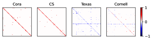
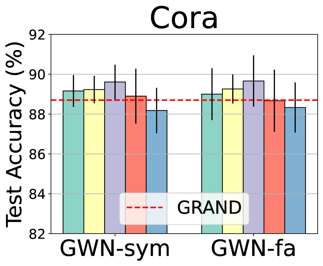
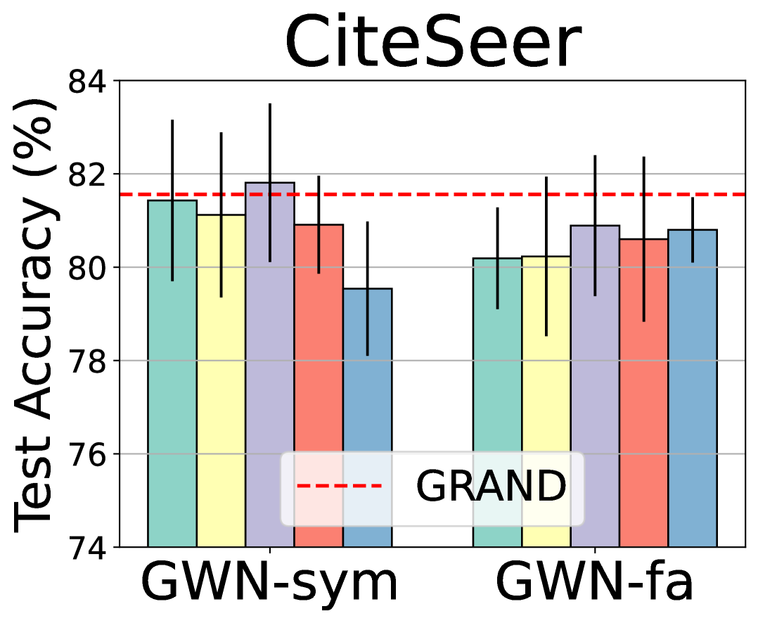
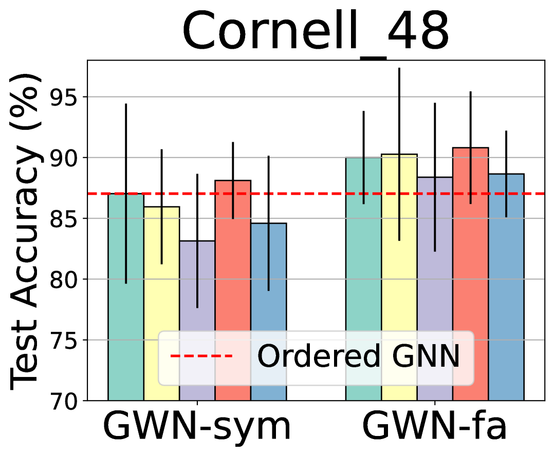
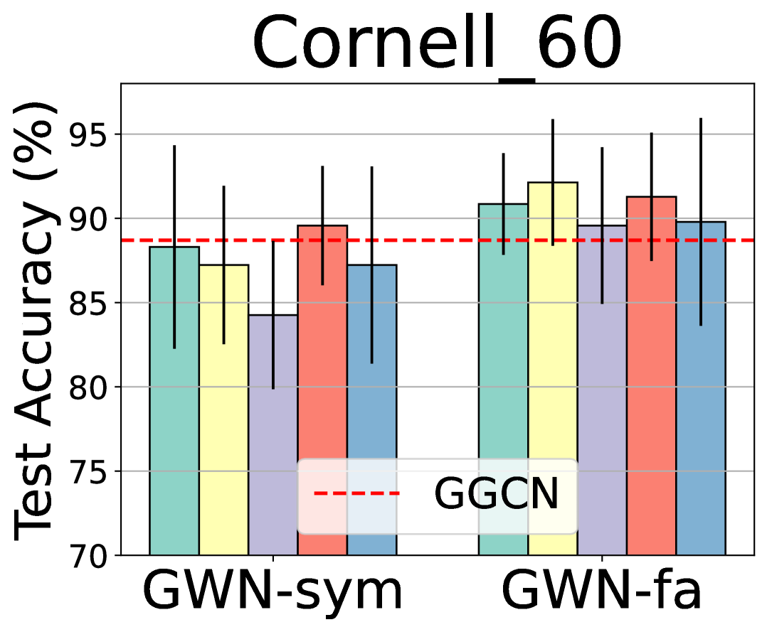
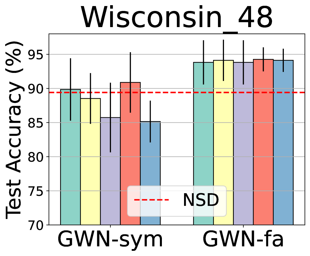
To validate the feasibility of GWN, we first compare it with GNNs based on differential equations on 6 homophilic graphs. Table 2 indicates that GWN outperforms heat equation based methods sush as GRAND on 5 datasets and achieves suboptimal performance on Photo. Since both GWN-sym and GWN-fa can be treated as low-pass filters, their performances are closely comparable. Then, we examine the generality of GWN on heterophilic graphs. Table 3 demonstrates that GWN outperforms state-of-the-art methods under two commonly used data splits. GWN-sym and GWN-fa show a significant difference on heterophilic graphs, which can be attributed to the high-pass filter of GWN-fa. It reflects remarkable performance in modelling heterophily in graphs. Next, we further probe whether the low-pass and high-pass filters in GWN-fa perform as expected. As shown in Figure 2, we visualize the attention matrix in Eq. (18). As stated in Sec. 3.4, GWN behaves as a low-pass filter when and behaves as a high-pass filter when . This is consistent with the visualized results. Additionally, it is worth noting that under the 48%/32%/20% split, GWN-fa even outperforms most state-of-the-art methods under the 60%/20%/20% split, highlighting its superiority in scenarios with low label rates. Furthermore, GWNs also achieve competitive performance on obgn-arxiv, demonstrating its scalability on large-scale graphs.


| Cora | CiteSeer | PubMed | Computers | Photo | CS | Texas | Cornell | Wisconsin | |
| GCN | 87.51 | 80.59 | 87.95 | 86.09 | 93.04 | 95.14 | 79.33 | 69.53 | 63.94 |
| GWN-sym | 89.61 ( 2.10) | 81.81 ( 1.22) | 90.56 ( 2.61) | 90.10 ( 4.01) | 95.31 ( 2.27) | 96.66 ( 1.52) | 91.64 ( 12.31) | 89.57 ( 20.04) | 93.38 ( 29.44) |
| FAGCN | 88.49 | 81.65 | 87.58 | 87.32 | 93.41 | 95.79 | 85.57 | 86.38 | 84.88 |
| GWN-fa | 89.66 ( 1.17) | 80.89 ( 0.76) | 90.64 ( 3.06) | 90.62 ( 3.30) | 95.61 ( 2.20) | 96.67 ( 0.88) | 93.28 ( 7.71) | 92.13 ( 5.75) | 95.63 ( 10.75) |
4.3. Over-smoothing Analysis
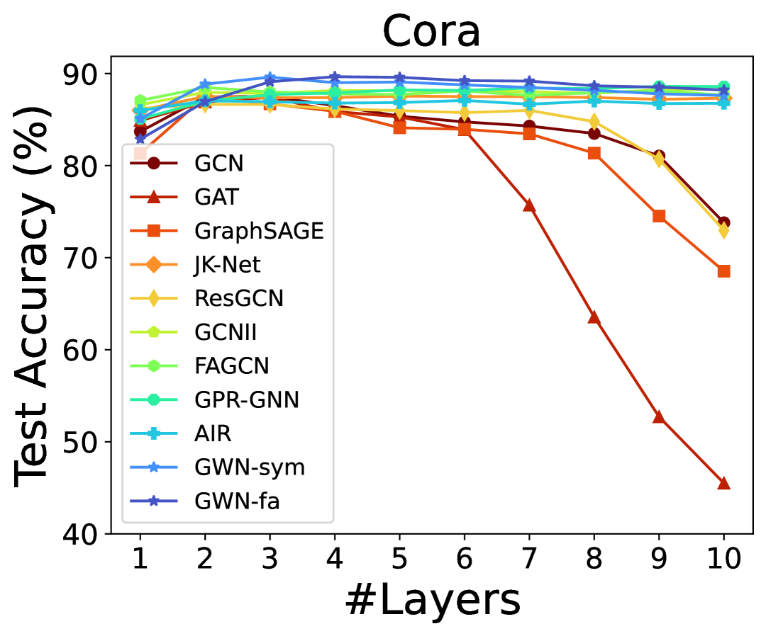
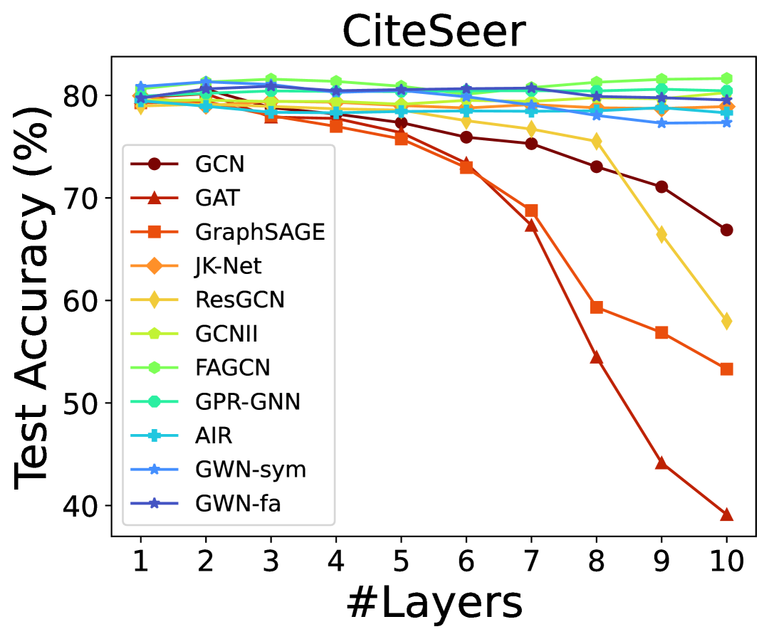
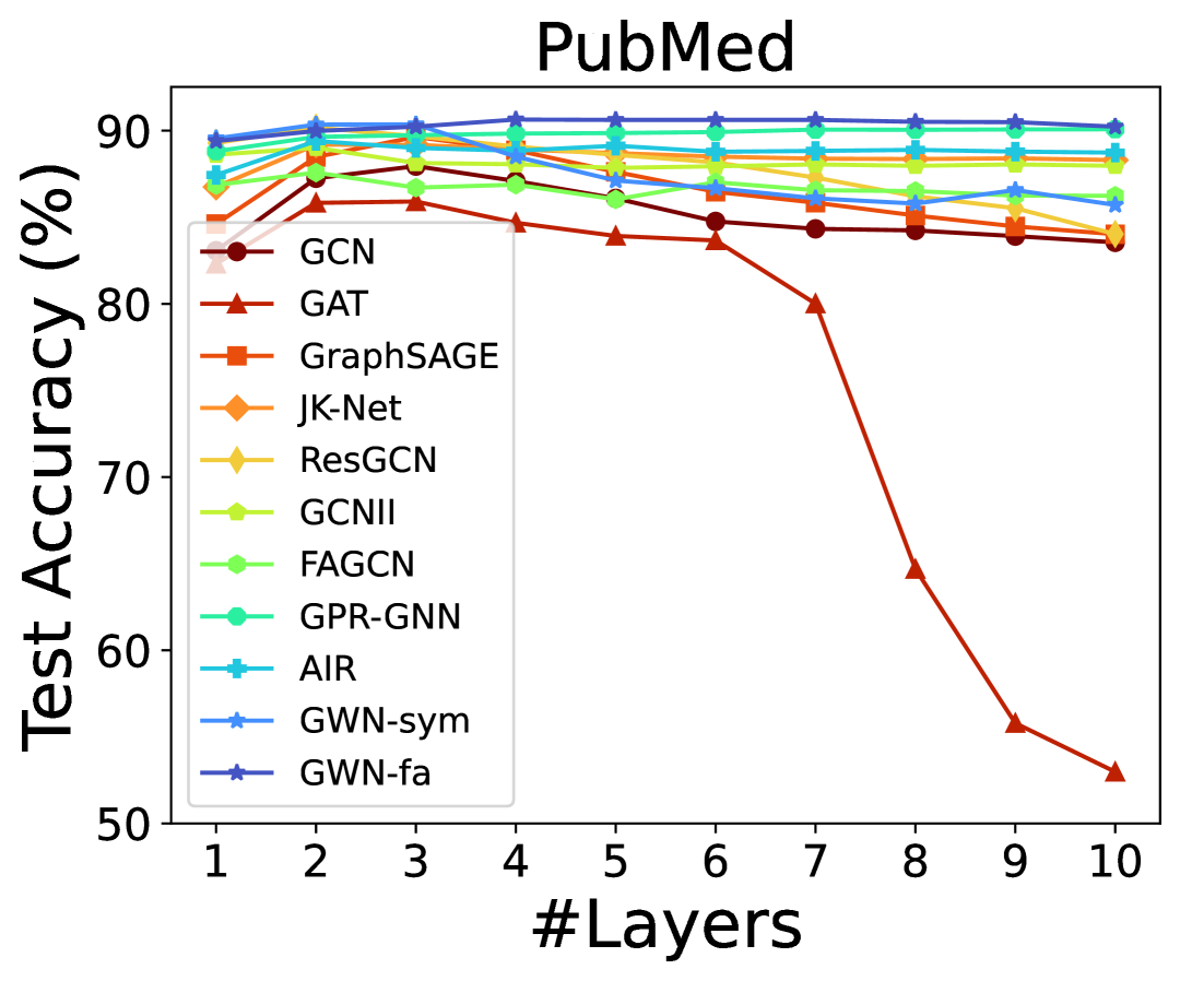
We investigate the ability of GWN to mitigate over-smoothing on three citation networks: Cora, CiteSeer, and PubMed. Following the practice of Chamberlain et al. (2021) and Rusch et al. (2022), we set , then the terminal time denotes the number of layers. Figure 3 demonstrates that compared to GNNs specifically designed for over-smoothing, GWN not only outperforms all baselines in terms of performance but also maintains its performance as the number of layers increases. It demonstrates that our models have better performance in mitigating the over-smoothing issue.
4.4. Stability Analysis
We analyze the stability of the explicit scheme in experiments. We run GWN on all datasets and report the accuracy for different . As depicted in Figure 4, on larger-scale datasets such as CS, GWN exhibits minimal performance differences when is varied. On smaller-scale datasets like Texas, due to the high-pass filters, GWN-fa demonstrates better stability compared to GWN-sym. Compared to GRAND, which only guarantees stability of the explicit scheme for (Chamberlain et al., 2021), GWN can maintain stability at larger while achieving higher computational efficiency and performance.
4.5. Analysis of base models
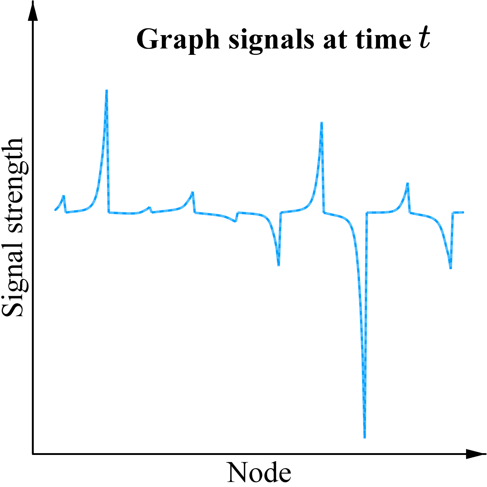
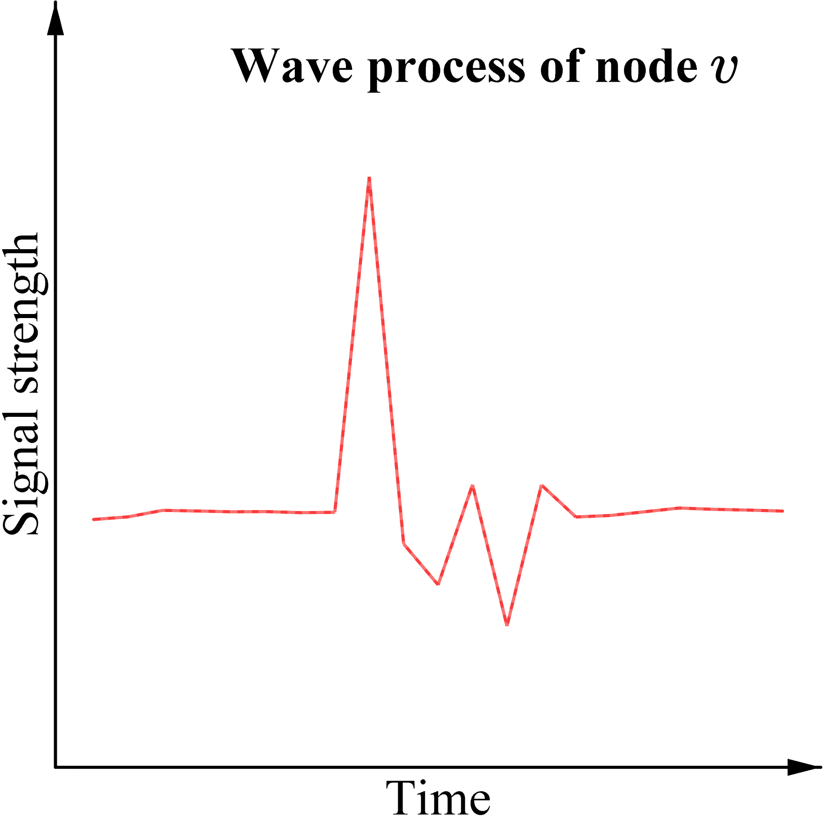
We explore the impact of base models in Table 4, where both GCN and FAGCN increase their performances in the form of the graph wave equation. Besides, we also show the visualization of wave propagation of GWN-sym and GWN-fa on Cora. From Figure 5, the waveform of GWN-sym are not prominent at early iterations, while the waveform of GWN-fa demonstrate more frequent information interactions at any time. Figure 6(a) depicts wave signals at a specific time, where the waveform of GWN-sym appears chaotic, whereas the waveform of GWN-fa is relatively clear. From Figure 6(b), compared to the waveform of GWN-sym, the waveform of GWN-fa exhibits periodic variations of peaks and troughs. We believe that these phenomena can be attributed to the ability of capturing both the low- and high-frequency signals in GWN-fa.
5. Related Work
Spectral GNNs.
Spectral GNNs (Bruna et al., 2014) based on Laplacian to design various filter functions in the spectral domain. One category of spectral GNNs directly modify the Laplacian. GCN (Kipf and Welling, 2017) incorporates self-loops in the normalized Laplacian, which manifests as a low-pass filter. Some methods (Bo et al., 2021; Luan et al., 2022; Zheng et al., 2021; Geng et al., 2023) introduce additional high-pass filters to learn difference between nodes. Bianchi et al. (2022) propose an auto-regressive moving average filter to capture the global graph structure. Defferrard et al. (2016) and He et al. (2022) approximate the spectral graph convolution using Chebyshev polynomial. He et al. (2021) approximate arbitrary filters using Bernstein polynomials. Wang and Zhang (2022) utilize Jacobi polynomials to adapt a wider range of weight functions. Chien et al. (2021) employ learnable parameters to approximate the polynomial coefficients. These methods are all built upon the traditional graph signal processing methods, but few of them fully explore the nature of wave propagation in the MP process.
Differential Equations on Graphs.
Neural ODE (Chen et al., 2018) models the embedding representation as a continuous dynamic with respect to neural network parameters. Poli et al. (2019) propose a continuous-depth GNN framework and solves the forward process using numerical methods. Xhonneux et al. (2020) establish the relationship between the derivative of node embeddings and the initial and neighboring embeddings of nodes. Rusch et al. (2022) relate to traditional GNNs using second-order ODEs. Nguyen et al. (2024) adapt well-known Kuramoto model to alleviate over-smoothing. Neural PDE (Li et al., 2020) applies partial differential equations to graph-based problems. Eliasof et al. (2021) utilizes non-linear diffusion and non-linear hyperbolic equations to model message passing. Wang et al. (2021) decouple the terminal time and feature propagation steps from a continuous perspective. Klicpera et al. (2019) define graph diffusion convolution to overcome the limitation of traditional GNNs in aggregating only direct neighbors. Zhao et al. (2021) propose adaptive diffusion convolution to automatically learn the optimal neighborhood from the data. Recent works introduce the heat diffusion equation on graphs to simulate the temporal dynamics of node embeddings (Chamberlain et al., 2021). The explicit scheme stability derived from GRAND is conditional, ensuring model performance only when using smaller time steps, leading to inefficient model performance. Thorpe et al. (2022) further utilize a heat diffusion equation with a source term to define graph convolution, which performs better in low-label-rate scenarios. Li et al. (2024) introduce a general diffusion equation framework with a fidelity term and establishes the connection between the diffusion process and GNNs. Compared to considering message passing as a heat diffusion process between nodes, treating it as a wave propagation process better aligns with the process of inter-node information interaction described in graph signal processing. Moreover, note that there are several DE-based GNNs (Xhonneux et al., 2020; Wang et al., 2021; Eliasof et al., 2021; Thorpe et al., 2022; Li et al., 2024) lack stability proofs, which can hardly ensure the robustness of models, and weaker stability conditions make it challenging to balance model performance and efficiency. In contrast, in this paper, the proposed graph wave networks can significantly enhance efficiency while ensuring model performance, due to its constantly stable properties.
(a) time view
(b) node view
6. Conclusion
In this paper, we consider the message passing in GNNs as a wave propagation process, and further develop graph wave networks (GWNs) based on the proposed graph wave equation with spectral GNNs. We demonstrate that compared to the heat equation, the graph wave equation exhibits superior performance and stability. Extensive experiments demonstrate that our GWNs obtain accurate and efficient performance, and show effectiveness in addressing challenging graph problems such as over-smoothing and heterophily modelling. Our future work would explore more complex and general Laplacian polynomials to advance GNNs.
Acknowledgements.
This work is supported by the National Natural Science Foundation of China (No.62406319 and No.62472416), the Youth Innovation Promotion Association of CAS (Grant No. 2021153), and the Postdoctoral Fellowship Program of CPSF (No.GZC20232968).References
- (1)
- Abu-El-Haija et al. (2019) Sami Abu-El-Haija, Bryan Perozzi, Amol Kapoor, Nazanin Alipourfard, Kristina Lerman, Hrayr Harutyunyan, Greg Ver Steeg, and Aram Galstyan. 2019. MixHop: Higher-Order Graph Convolutional Architectures via Sparsified Neighborhood Mixing. In Proceedings of the 36th International Conference on Machine Learning, ICML 2019, 9-15 June 2019, Long Beach, California, USA. PMLR.
- Bianchi et al. (2022) Filippo Maria Bianchi, Daniele Grattarola, Lorenzo Livi, and Cesare Alippi. 2022. Graph Neural Networks With Convolutional ARMA Filters. IEEE Trans. Pattern Anal. Mach. Intell. 44, 7 (2022), 3496–3507. doi:10.1109/TPAMI.2021.3054830
- Bo et al. (2021) Deyu Bo, Xiao Wang, Chuan Shi, and Huawei Shen. 2021. Beyond Low-frequency Information in Graph Convolutional Networks. In Thirty-Fifth AAAI Conference on Artificial Intelligence, AAAI 2021, Thirty-Third Conference on Innovative Applications of Artificial Intelligence, IAAI 2021, The Eleventh Symposium on Educational Advances in Artificial Intelligence, EAAI 2021, Virtual Event, February 2-9, 2021. AAAI Press.
- Bodnar et al. (2022) Cristian Bodnar, Francesco Di Giovanni, Benjamin Paul Chamberlain, Pietro Lió, and Michael M. Bronstein. 2022. Neural Sheaf Diffusion: A Topological Perspective on Heterophily and Oversmoothing in GNNs. In NeurIPS.
- Bruna et al. (2014) Joan Bruna, Wojciech Zaremba, Arthur Szlam, and Yann LeCun. 2014. Spectral Networks and Locally Connected Networks on Graphs. In 2nd International Conference on Learning Representations, ICLR 2014, Banff, AB, Canada, April 14-16, 2014, Conference Track Proceedings, Yoshua Bengio and Yann LeCun (Eds.). http://arxiv.org/abs/1312.6203
- Chamberlain et al. (2021) Ben Chamberlain, James Rowbottom, Maria I. Gorinova, Michael M. Bronstein, Stefan Webb, and Emanuele Rossi. 2021. GRAND: Graph Neural Diffusion. In Proceedings of the 38th International Conference on Machine Learning, ICML 2021, 18-24 July 2021, Virtual Event (Proceedings of Machine Learning Research, Vol. 139), Marina Meila and Tong Zhang (Eds.). PMLR, 1407–1418. http://proceedings.mlr.press/v139/chamberlain21a.html
- Chen et al. (2020) Ming Chen, Zhewei Wei, Zengfeng Huang, Bolin Ding, and Yaliang Li. 2020. Simple and Deep Graph Convolutional Networks. In Proceedings of the 37th International Conference on Machine Learning, ICML 2020, 13-18 July 2020, Virtual Event. PMLR.
- Chen et al. (2018) Tian Qi Chen, Yulia Rubanova, Jesse Bettencourt, and David Duvenaud. 2018. Neural Ordinary Differential Equations. In Advances in Neural Information Processing Systems 31: Annual Conference on Neural Information Processing Systems 2018, NeurIPS 2018, December 3-8, 2018, Montréal, Canada, Samy Bengio, Hanna M. Wallach, Hugo Larochelle, Kristen Grauman, Nicolò Cesa-Bianchi, and Roman Garnett (Eds.). 6572–6583. https://proceedings.neurips.cc/paper/2018/hash/69386f6bb1dfed68692a24c8686939b9-Abstract.html
- Chien et al. (2021) Eli Chien, Jianhao Peng, Pan Li, and Olgica Milenkovic. 2021. Adaptive Universal Generalized PageRank Graph Neural Network. In 9th International Conference on Learning Representations, ICLR 2021, Virtual Event, Austria, May 3-7, 2021. OpenReview.net.
- Defferrard et al. (2016) Michaël Defferrard, Xavier Bresson, and Pierre Vandergheynst. 2016. Convolutional Neural Networks on Graphs with Fast Localized Spectral Filtering. In Advances in Neural Information Processing Systems 29: Annual Conference on Neural Information Processing Systems 2016, December 5-10, 2016, Barcelona, Spain.
- Eliasof et al. (2021) Moshe Eliasof, Eldad Haber, and Eran Treister. 2021. PDE-GCN: Novel Architectures for Graph Neural Networks Motivated by Partial Differential Equations. In Advances in Neural Information Processing Systems 34: Annual Conference on Neural Information Processing Systems 2021, NeurIPS 2021, December 6-14, 2021, virtual, Marc’Aurelio Ranzato, Alina Beygelzimer, Yann N. Dauphin, Percy Liang, and Jennifer Wortman Vaughan (Eds.). 3836–3849. https://proceedings.neurips.cc/paper/2021/hash/1f9f9d8ff75205aa73ec83e543d8b571-Abstract.html
- Fey and Lenssen (2019) Matthias Fey and Jan Eric Lenssen. 2019. Fast Graph Representation Learning with PyTorch Geometric. In ICLR Workshop on Representation Learning on Graphs and Manifolds.
- Gaudelet et al. (2021) Thomas Gaudelet, Ben Day, Arian R. Jamasb, Jyothish Soman, Cristian Regep, Gertrude Liu, Jeremy B. R. Hayter, Richard Vickers, Charles Roberts, Jian Tang, David Roblin, Tom L. Blundell, Michael M. Bronstein, and Jake P. Taylor-King. 2021. Utilizing graph machine learning within drug discovery and development. Briefings Bioinform. 22, 6 (2021). doi:10.1093/BIB/BBAB159
- Geng et al. (2023) Haoyu Geng, Chao Chen, Yixuan He, Gang Zeng, Zhaobing Han, Hua Chai, and Junchi Yan. 2023. Pyramid Graph Neural Network: A Graph Sampling and Filtering Approach for Multi-scale Disentangled Representations. In Proceedings of the 29th ACM SIGKDD Conference on Knowledge Discovery and Data Mining, KDD 2023, Long Beach, CA, USA, August 6-10, 2023, Ambuj K. Singh, Yizhou Sun, Leman Akoglu, Dimitrios Gunopulos, Xifeng Yan, Ravi Kumar, Fatma Ozcan, and Jieping Ye (Eds.). ACM, 518–530. doi:10.1145/3580305.3599478
- Hamilton et al. (2017) William L. Hamilton, Zhitao Ying, and Jure Leskovec. 2017. Inductive Representation Learning on Large Graphs. In Advances in Neural Information Processing Systems 30: Annual Conference on Neural Information Processing Systems 2017, December 4-9, 2017, Long Beach, CA, USA.
- He et al. (2021) Mingguo He, Zhewei Wei, Zengfeng Huang, and Hongteng Xu. 2021. BernNet: Learning Arbitrary Graph Spectral Filters via Bernstein Approximation. In Advances in Neural Information Processing Systems 34: Annual Conference on Neural Information Processing Systems 2021, NeurIPS 2021, December 6-14, 2021, virtual, Marc’Aurelio Ranzato, Alina Beygelzimer, Yann N. Dauphin, Percy Liang, and Jennifer Wortman Vaughan (Eds.). 14239–14251. https://proceedings.neurips.cc/paper/2021/hash/76f1cfd7754a6e4fc3281bcccb3d0902-Abstract.html
- He et al. (2022) Mingguo He, Zhewei Wei, and Ji-Rong Wen. 2022. Convolutional Neural Networks on Graphs with Chebyshev Approximation, Revisited. In Advances in Neural Information Processing Systems 35: Annual Conference on Neural Information Processing Systems 2022, NeurIPS 2022, New Orleans, LA, USA, November 28 - December 9, 2022, Sanmi Koyejo, S. Mohamed, A. Agarwal, Danielle Belgrave, K. Cho, and A. Oh (Eds.). http://papers.nips.cc/paper_files/paper/2022/hash/2f9b3ee2bcea04b327c09d7e3145bd1e-Abstract-Conference.html
- Hu et al. (2020) Weihua Hu, Matthias Fey, Marinka Zitnik, Yuxiao Dong, Hongyu Ren, Bowen Liu, Michele Catasta, and Jure Leskovec. 2020. Open Graph Benchmark: Datasets for Machine Learning on Graphs. In Advances in Neural Information Processing Systems 33: Annual Conference on Neural Information Processing Systems 2020, NeurIPS 2020, December 6-12, 2020, virtual, Hugo Larochelle, Marc’Aurelio Ranzato, Raia Hadsell, Maria-Florina Balcan, and Hsuan-Tien Lin (Eds.). https://proceedings.neurips.cc/paper/2020/hash/fb60d411a5c5b72b2e7d3527cfc84fd0-Abstract.html
- Kingma and Ba (2015) Diederik P. Kingma and Jimmy Ba. 2015. Adam: A Method for Stochastic Optimization. In 3rd International Conference on Learning Representations, ICLR 2015, San Diego, CA, USA, May 7-9, 2015, Conference Track Proceedings.
- Kipf and Welling (2017) Thomas N. Kipf and Max Welling. 2017. Semi-Supervised Classification with Graph Convolutional Networks. In 5th International Conference on Learning Representations, ICLR 2017, Toulon, France, April 24-26, 2017, Conference Track Proceedings. OpenReview.net.
- Klicpera et al. (2019) Johannes Klicpera, Stefan Weißenberger, and Stephan Günnemann. 2019. Diffusion Improves Graph Learning. In Advances in Neural Information Processing Systems 32: Annual Conference on Neural Information Processing Systems 2019, NeurIPS 2019, December 8-14, 2019, Vancouver, BC, Canada, Hanna M. Wallach, Hugo Larochelle, Alina Beygelzimer, Florence d’Alché-Buc, Emily B. Fox, and Roman Garnett (Eds.). 13333–13345. https://proceedings.neurips.cc/paper/2019/hash/23c894276a2c5a16470e6a31f4618d73-Abstract.html
- Li et al. (2019) Guohao Li, Matthias Müller, Ali K. Thabet, and Bernard Ghanem. 2019. DeepGCNs: Can GCNs Go As Deep As CNNs?. In 2019 IEEE/CVF International Conference on Computer Vision, ICCV 2019, Seoul, Korea (South), October 27 - November 2, 2019. IEEE, 9266–9275. doi:10.1109/ICCV.2019.00936
- Li et al. (2022) Xiang Li, Renyu Zhu, Yao Cheng, Caihua Shan, Siqiang Luo, Dongsheng Li, and Weining Qian. 2022. Finding Global Homophily in Graph Neural Networks When Meeting Heterophily. In International Conference on Machine Learning, ICML 2022, 17-23 July 2022, Baltimore, Maryland, USA (Proceedings of Machine Learning Research, Vol. 162), Kamalika Chaudhuri, Stefanie Jegelka, Le Song, Csaba Szepesvári, Gang Niu, and Sivan Sabato (Eds.). PMLR, 13242–13256. https://proceedings.mlr.press/v162/li22ad.html
- Li et al. (2024) Yibo Li, Xiao Wang, Hongrui Liu, and Chuan Shi. 2024. A Generalized Neural Diffusion Framework on Graphs. In Thirty-Eighth AAAI Conference on Artificial Intelligence, AAAI 2024, Thirty-Sixth Conference on Innovative Applications of Artificial Intelligence, IAAI 2024, Fourteenth Symposium on Educational Advances in Artificial Intelligence, EAAI 2014, February 20-27, 2024, Vancouver, Canada, Michael J. Wooldridge, Jennifer G. Dy, and Sriraam Natarajan (Eds.). AAAI Press, 8707–8715. doi:10.1609/AAAI.V38I8.28716
- Li et al. (2020) Zongyi Li, Nikola B. Kovachki, Kamyar Azizzadenesheli, Burigede Liu, Andrew M. Stuart, Kaushik Bhattacharya, and Anima Anandkumar. 2020. Multipole Graph Neural Operator for Parametric Partial Differential Equations. In Advances in Neural Information Processing Systems 33: Annual Conference on Neural Information Processing Systems 2020, NeurIPS 2020, December 6-12, 2020, virtual, Hugo Larochelle, Marc’Aurelio Ranzato, Raia Hadsell, Maria-Florina Balcan, and Hsuan-Tien Lin (Eds.). https://proceedings.neurips.cc/paper/2020/hash/4b21cf96d4cf612f239a6c322b10c8fe-Abstract.html
- Lim et al. (2021) Derek Lim, Felix Hohne, Xiuyu Li, Sijia Linda Huang, Vaishnavi Gupta, Omkar Bhalerao, and Ser-Nam Lim. 2021. Large Scale Learning on Non-Homophilous Graphs: New Benchmarks and Strong Simple Methods. In Advances in Neural Information Processing Systems 34: Annual Conference on Neural Information Processing Systems 2021, NeurIPS 2021, December 6-14, 2021, virtual, Marc’Aurelio Ranzato, Alina Beygelzimer, Yann N. Dauphin, Percy Liang, and Jennifer Wortman Vaughan (Eds.). 20887–20902. https://proceedings.neurips.cc/paper/2021/hash/ae816a80e4c1c56caa2eb4e1819cbb2f-Abstract.html
- Lin et al. (2021) Jianghao Lin, Weiwen Liu, Xinyi Dai, Weinan Zhang, Shuai Li, Ruiming Tang, Xiuqiang He, Jianye Hao, and Yong Yu. 2021. A Graph-Enhanced Click Model for Web Search. In SIGIR ’21: The 44th International ACM SIGIR Conference on Research and Development in Information Retrieval, Virtual Event, Canada, July 11-15, 2021, Fernando Diaz, Chirag Shah, Torsten Suel, Pablo Castells, Rosie Jones, and Tetsuya Sakai (Eds.). ACM, 1259–1268. doi:10.1145/3404835.3462895
- Liu et al. (2022) Meng Liu, Zhengyang Wang, and Shuiwang Ji. 2022. Non-Local Graph Neural Networks. IEEE Trans. Pattern Anal. Mach. Intell. 44, 12 (2022), 10270–10276. doi:10.1109/TPAMI.2021.3134200
- Luan et al. (2022) Sitao Luan, Chenqing Hua, Qincheng Lu, Jiaqi Zhu, Mingde Zhao, Shuyuan Zhang, Xiao-Wen Chang, and Doina Precup. 2022. Revisiting Heterophily For Graph Neural Networks. In NeurIPS.
- Nguyen et al. (2024) Tuan Nguyen, Hirotada Honda, Takashi Sano, Vinh Nguyen, Shugo Nakamura, and Tan Minh Nguyen. 2024. From Coupled Oscillators to Graph Neural Networks: Reducing Over-smoothing via a Kuramoto Model-based Approach. In International Conference on Artificial Intelligence and Statistics, 2-4 May 2024, Palau de Congressos, Valencia, Spain (Proceedings of Machine Learning Research, Vol. 238), Sanjoy Dasgupta, Stephan Mandt, and Yingzhen Li (Eds.). PMLR, 2710–2718. https://proceedings.mlr.press/v238/nguyen24c.html
- Pei et al. (2020) Hongbin Pei, Bingzhe Wei, Kevin Chen-Chuan Chang, Yu Lei, and Bo Yang. 2020. Geom-GCN: Geometric Graph Convolutional Networks. In 8th International Conference on Learning Representations, ICLR 2020, Addis Ababa, Ethiopia, April 26-30, 2020. OpenReview.net.
- Poli et al. (2019) Michael Poli, Stefano Massaroli, Junyoung Park, Atsushi Yamashita, Hajime Asama, and Jinkyoo Park. 2019. Graph Neural Ordinary Differential Equations. CoRR abs/1911.07532 (2019). arXiv:1911.07532 http://arxiv.org/abs/1911.07532
- Rozemberczki et al. (2019) Benedek Rozemberczki, Carl Allen, and Rik Sarkar. 2019. Multi-scale Attributed Node Embedding. CoRR abs/1909.13021 (2019). arXiv:1909.13021
- Rozemberczki and Sarkar (2020a) Benedek Rozemberczki and Rik Sarkar. 2020a. Characteristic Functions on Graphs: Birds of a Feather, from Statistical Descriptors to Parametric Models. In CIKM ’20: The 29th ACM International Conference on Information and Knowledge Management, Virtual Event, Ireland, October 19-23, 2020. ACM. doi:10.1145/3340531.3411866
- Rozemberczki and Sarkar (2020b) Benedek Rozemberczki and Rik Sarkar. 2020b. Characteristic Functions on Graphs: Birds of a Feather, from Statistical Descriptors to Parametric Models. In CIKM ’20: The 29th ACM International Conference on Information and Knowledge Management, Virtual Event, Ireland, October 19-23, 2020. ACM. doi:10.1145/3340531.3411866
- Rusch et al. (2022) T. Konstantin Rusch, Ben Chamberlain, James Rowbottom, Siddhartha Mishra, and Michael M. Bronstein. 2022. Graph-Coupled Oscillator Networks. In International Conference on Machine Learning, ICML 2022, 17-23 July 2022, Baltimore, Maryland, USA (Proceedings of Machine Learning Research, Vol. 162), Kamalika Chaudhuri, Stefanie Jegelka, Le Song, Csaba Szepesvári, Gang Niu, and Sivan Sabato (Eds.). PMLR, 18888–18909. https://proceedings.mlr.press/v162/rusch22a.html
- Shchur et al. (2018) Oleksandr Shchur, Maximilian Mumme, Aleksandar Bojchevski, and Stephan Günnemann. 2018. Pitfalls of Graph Neural Network Evaluation. CoRR abs/1811.05868 (2018). arXiv:1811.05868
- Shlomi et al. (2021) Jonathan Shlomi, Peter W. Battaglia, and Jean-Roch Vlimant. 2021. Graph neural networks in particle physics. Mach. Learn. Sci. Technol. 2, 2 (2021), 21001. doi:10.1088/2632-2153/ABBF9A
- Shuman et al. (2013) David I. Shuman, Sunil K. Narang, Pascal Frossard, Antonio Ortega, and Pierre Vandergheynst. 2013. The Emerging Field of Signal Processing on Graphs: Extending High-Dimensional Data Analysis to Networks and Other Irregular Domains. IEEE Signal Process. Mag. 30, 3 (2013), 83–98. doi:10.1109/MSP.2012.2235192
- Song et al. (2023) Yunchong Song, Chenghu Zhou, Xinbing Wang, and Zhouhan Lin. 2023. Ordered GNN: Ordering Message Passing to Deal with Heterophily and Over-smoothing. In The Eleventh International Conference on Learning Representations, ICLR 2023, Kigali, Rwanda, May 1-5, 2023. OpenReview.net. https://openreview.net/pdf?id=wKPmPBHSnT6
- Suresh et al. (2021) Susheel Suresh, Vinith Budde, Jennifer Neville, Pan Li, and Jianzhu Ma. 2021. Breaking the Limit of Graph Neural Networks by Improving the Assortativity of Graphs with Local Mixing Patterns. In KDD ’21: The 27th ACM SIGKDD Conference on Knowledge Discovery and Data Mining, Virtual Event, Singapore, August 14-18, 2021, Feida Zhu, Beng Chin Ooi, and Chunyan Miao (Eds.). ACM, 1541–1551. doi:10.1145/3447548.3467373
- Thorpe et al. (2022) Matthew Thorpe, Tan Minh Nguyen, Hedi Xia, Thomas Strohmer, Andrea L. Bertozzi, Stanley J. Osher, and Bao Wang. 2022. GRAND++: Graph Neural Diffusion with A Source Term. In The Tenth International Conference on Learning Representations, ICLR 2022, Virtual Event, April 25-29, 2022. OpenReview.net. https://openreview.net/forum?id=EMxu-dzvJk
- Velickovic et al. (2018) Petar Velickovic, Guillem Cucurull, Arantxa Casanova, Adriana Romero, Pietro Liò, and Yoshua Bengio. 2018. Graph Attention Networks. In 6th International Conference on Learning Representations, ICLR 2018, Vancouver, BC, Canada, April 30 - May 3, 2018, Conference Track Proceedings. OpenReview.net.
- Wang and Zhang (2022) Xiyuan Wang and Muhan Zhang. 2022. How Powerful are Spectral Graph Neural Networks. In International Conference on Machine Learning, ICML 2022, 17-23 July 2022, Baltimore, Maryland, USA (Proceedings of Machine Learning Research, Vol. 162), Kamalika Chaudhuri, Stefanie Jegelka, Le Song, Csaba Szepesvári, Gang Niu, and Sivan Sabato (Eds.). PMLR, 23341–23362. https://proceedings.mlr.press/v162/wang22am.html
- Wang et al. (2021) Yifei Wang, Yisen Wang, Jiansheng Yang, and Zhouchen Lin. 2021. Dissecting the Diffusion Process in Linear Graph Convolutional Networks. In Advances in Neural Information Processing Systems 34: Annual Conference on Neural Information Processing Systems 2021, NeurIPS 2021, December 6-14, 2021, virtual, Marc’Aurelio Ranzato, Alina Beygelzimer, Yann N. Dauphin, Percy Liang, and Jennifer Wortman Vaughan (Eds.). 5758–5769. https://proceedings.neurips.cc/paper/2021/hash/2d95666e2649fcfc6e3af75e09f5adb9-Abstract.html
- Wu et al. (2019) Felix Wu, Amauri H. Souza Jr., Tianyi Zhang, Christopher Fifty, Tao Yu, and Kilian Q. Weinberger. 2019. Simplifying Graph Convolutional Networks. In Proceedings of the 36th International Conference on Machine Learning, ICML 2019, 9-15 June 2019, Long Beach, California, USA. PMLR.
- Wu et al. (2023) Shiwen Wu, Fei Sun, Wentao Zhang, Xu Xie, and Bin Cui. 2023. Graph Neural Networks in Recommender Systems: A Survey. ACM Comput. Surv. 55, 5 (2023), 97:1–97:37. doi:10.1145/3535101
- Wu et al. (2021) Zonghan Wu, Shirui Pan, Fengwen Chen, Guodong Long, Chengqi Zhang, and Philip S. Yu. 2021. A Comprehensive Survey on Graph Neural Networks. IEEE Trans. Neural Networks Learn. Syst. 32, 1 (2021), 4–24. doi:10.1109/TNNLS.2020.2978386
- Xhonneux et al. (2020) Louis-Pascal A. C. Xhonneux, Meng Qu, and Jian Tang. 2020. Continuous Graph Neural Networks. In Proceedings of the 37th International Conference on Machine Learning, ICML 2020, 13-18 July 2020, Virtual Event (Proceedings of Machine Learning Research, Vol. 119). PMLR, 10432–10441. http://proceedings.mlr.press/v119/xhonneux20a.html
- Xu et al. (2018) Keyulu Xu, Chengtao Li, Yonglong Tian, Tomohiro Sonobe, Ken-ichi Kawarabayashi, and Stefanie Jegelka. 2018. Representation Learning on Graphs with Jumping Knowledge Networks. In Proceedings of the 35th International Conference on Machine Learning, ICML 2018, Stockholmsmässan, Stockholm, Sweden, July 10-15, 2018. PMLR.
- Yan et al. (2022) Yujun Yan, Milad Hashemi, Kevin Swersky, Yaoqing Yang, and Danai Koutra. 2022. Two Sides of the Same Coin: Heterophily and Oversmoothing in Graph Convolutional Neural Networks. In IEEE International Conference on Data Mining, ICDM 2022, Orlando, FL, USA, November 28 - Dec. 1, 2022. IEEE. doi:10.1109/ICDM54844.2022.00169
- Yang et al. (2016) Zhilin Yang, William W. Cohen, and Ruslan Salakhutdinov. 2016. Revisiting Semi-Supervised Learning with Graph Embeddings. In Proceedings of the 33nd International Conference on Machine Learning, ICML 2016, New York City, NY, USA, June 19-24, 2016. JMLR.org.
- Zhang et al. (2022) Wentao Zhang, Zeang Sheng, Ziqi Yin, Yuezihan Jiang, Yikuan Xia, Jun Gao, Zhi Yang, and Bin Cui. 2022. Model Degradation Hinders Deep Graph Neural Networks. In KDD ’22: The 28th ACM SIGKDD Conference on Knowledge Discovery and Data Mining, Washington, DC, USA, August 14 - 18, 2022, Aidong Zhang and Huzefa Rangwala (Eds.). ACM, 2493–2503. doi:10.1145/3534678.3539374
- Zhao et al. (2021) Jialin Zhao, Yuxiao Dong, Ming Ding, Evgeny Kharlamov, and Jie Tang. 2021. Adaptive Diffusion in Graph Neural Networks. In Advances in Neural Information Processing Systems 34: Annual Conference on Neural Information Processing Systems 2021, NeurIPS 2021, December 6-14, 2021, virtual, Marc’Aurelio Ranzato, Alina Beygelzimer, Yann N. Dauphin, Percy Liang, and Jennifer Wortman Vaughan (Eds.). 23321–23333. https://proceedings.neurips.cc/paper/2021/hash/c42af2fa7356818e0389593714f59b52-Abstract.html
- Zheng et al. (2021) Xuebin Zheng, Bingxin Zhou, Junbin Gao, Yuguang Wang, Pietro Lió, Ming Li, and Guido Montúfar. 2021. How Framelets Enhance Graph Neural Networks. In Proceedings of the 38th International Conference on Machine Learning, ICML 2021, 18-24 July 2021, Virtual Event (Proceedings of Machine Learning Research, Vol. 139), Marina Meila and Tong Zhang (Eds.). PMLR, 12761–12771. http://proceedings.mlr.press/v139/zheng21c.html
- Zhu et al. (2020) Jiong Zhu, Yujun Yan, Lingxiao Zhao, Mark Heimann, Leman Akoglu, and Danai Koutra. 2020. Beyond Homophily in Graph Neural Networks: Current Limitations and Effective Designs. In Advances in Neural Information Processing Systems 33: Annual Conference on Neural Information Processing Systems 2020, NeurIPS 2020, December 6-12, 2020, virtual.
Appendix A Detailed mathematical derivation
A.1. Proof of Proposition 1
Proof.
Since , then
| (19) |
where , if ; , otherwise. Hence, the graph wave equation can be rewritten as:
| (20) |
∎
A.2. Derivation of Explicit Scheme
For any node at time , we first discretize as . Then, considering its node representation along with a time step , its time difference of wave equation is given by:
| (21) |
where denotes the element of . Moreover, we can expand at point using Taylor series, and obtain
| (22) |
By substituting Eq. (21) into Eq. (22), we obtain
| (23) |
where denotes the truncation error. By truncating it, we obtain the forward time difference
| (24) |
where denotes the approximate value of at . Transforming the Eq. (24) into matrix form
| (25) |
We define the problem of solving the partial differential equation as an initial value problem, with the initial values given by the second-order central difference quotient:
| (26) |
| (27) |
where and can be obtained through neural layers. Let , then
| (28) |
By eliminating using the initial value Eq. (27), we obtain the node representation at time :
| (29) |
Finally, we can derive the node representation at time :
| (30) |
A.3. Proof of Theorem 2
According to Theorem 1, to prove the stability of the explicit scheme , we would like to prove that .
Proof.
To facilitate the stability analysis of the explicit scheme , we first need to transform it into the form of . Therefore, we assume
| (31) |
then, we can obtain the system of linear equations:
| (32) |
According the equation of the explicit scheme, we can obtain the values of each block matrix in :
| (33) |
resulting in as follows:
| (34) |
According to the Theorem 1, now we only need to compute the spectral radius of matrix to determine the condition that ensures the stability of the explicit scheme.
For convenience, we still use instead of , and let denote the eigenvalue of , respectively. Then, the characteristic determinant of is given by:
| (35) |
Evidently, is the characteristic equation of , with the eigenvalue . According to the ’s eigenvalue belongs to the interval , then . Next, we will investigate the range of values for .
Considering the equation obtained from :
| (36) |
If , that is , then the equation has a pair of complex conjugate roots and . And if , that is , then the equation has a pair of real roots and . We next discuss whether the satisfies for different , considering different cases.
Case 1. If .
a) When , the equation has a pair of complex conjugate roots . Evidently, . Therefore, for any , .
b) When , the equation has a pair of real roots .
As shown in Figure 7 (Left), when , , can take any positive real number at .
As shown in Figure 7 (Right), when , , can take any positive real number at .
Caes 2. If .
a) When , the equation has a pair of real roots .
As shown in Figure 7 (Left), when , , can take any positive real number at .
As shown in Figure 7 (Right), when , , can take any positive real number at .
b) When , the equation has a pair of complex conjugate roots . Evidently, . Therefore, for any , .
c) When , the equation has a pair of real roots .
As shown in Figure 7 (Left), when , , can take any positive real number at .
As shown in Figure 7 (Right), when , , can take any positive real number at .
In conclusion, when , the eigenvalues of satisfy , then the explicit scheme based on symmetric normalized Laplacian is constantly stable. ∎
A.4. Derivation of GWN-fa
Given frequency adaptive Laplacian as follow:
| (37) |
where is a low-pass filter, and is a high-pass filter. Based on the aforementioned two Laplacian, we can capture the low-frequency and high-frequency signals at time :
| (38) |
Then, we adaptively combine low-frequency and high-frequency signals using attention weights and obtain the feature vector of node at time :
| (39) |
where denotes the degree of node . Let and , we have
| (40) |
Weight can denote the correlation between nodes and , and it is computed using attention mechanism, where is a learnable parameter vector. Since is a learnable parameter, we can simplify as . Furthermore, in order to preserve the original node features, we replace with (Bo et al., 2021). So we can obtain
| (41) |
Rewrite Eq. (41) in matrix form
| (42) |
where the is the element of .
A.5. Proof of Theorem 3
Similar to the proof of Theorem 2 (in A.3), we prove the stability of frequency adaptive Laplacian.
Proof.
Given , we have
| (43) |
and its eigenvalues satisfy .
According to the proof of Theorem 1, when ’s eigenvalue belongs to the interval , then the eigenvalue of satisfies . Next, we will investigate the range of values for .
Considering the equation obtained from :
| (44) |
If , that is , then the equation has a pair of complex conjugate roots and . And if , that is , then the equation has real roots and . We next discuss whether the satisfies for different , considering different cases.
Case 1. If .
a) When , the equation has a pair of complex conjugate roots . Evidently, . Therefore, for any , .
b) When , the equation has a pair of real roots .
As shown in Figure 7 (Left), when , , can take any positive real number at .
As shown in Figure 7 (Right), when , , can take any positive real number at .
Caes 2. If .
a) When , the equation has a pair of real roots .
As shown in Figure 7 (Left), when , , can take any positive real number at .
As shown in Figure 7 (Right), when , , can take any positive real number at .
b) When , the equation has a pair of complex conjugate roots . Evidently, . Therefore, for any , .
c) When , the equation has a pair of real roots .
As shown in Figure 7 (Left), when , , can take any positive real number at .
As shown in Figure 7 (Right), when , , can take any positive real number at .
In conclusion, when , the eigenvalues of satisfy , then the explicit scheme based on frequency adaptive Laplacian is constantly stable. ∎
Appendix B Implementation Details
For all experiments, each method was run on a single NVIDIA Tesla V100 GPU with 16GB memory, and the CPU used is Intel Xeon E5-2660 v4 CPUs. All models train 200 epochs and employed an early stopping strategy triggered when the loss exceed the average loss of the last 10 epochs.
B.1. Dataset Statistics
Table 5 report the statistical information of datasets used in this paper.
| Datesets | #Nodes | #Edges | #Features | #Classes |
| Cora | 2708 | 5278 | 1433 | 7 |
| CiteSeer | 3327 | 4552 | 3703 | 6 |
| PubMed | 19717 | 44324 | 500 | 3 |
| Computers | 13752 | 245861 | 767 | 10 |
| Photo | 7650 | 119081 | 745 | 8 |
| CS | 18333 | 81894 | 6805 | 15 |
| Actor | 7600 | 30019 | 932 | 5 |
| Texas | 183 | 325 | 1703 | 5 |
| Cornell | 183 | 298 | 1703 | 5 |
| Wisconsin | 251 | 515 | 1703 | 5 |
| DeezerEurope | 28281 | 92752 | 128 | 2 |
| ogbn-arxiv | 169343 | 1166243 | 128 | 40 |
B.2. Parameter Search
We employ the wandb library for parameter search with Bayes scheme. The ranges for each hyperparameter are outlined in Table 6.
| Parameters | Range | Distribution |
| Dimension | set | |
| Time size | set | |
| Terminal time | uniform | |
| Dropout | uniform | |
| Learning rate | log_uniform_values | |
| Weight decay | uniform |
Appendix C Performance and Efficiency Analysis
| Datesets | Cora | CiteSeer | PubMed | Computers | Photo | CS |
| SGC | 86.10 1.37 (0.7) | 80.35 1.33 (0.7) | 83.45 0.51 (0.8) | 84.45 0.56 (0.7) | 88.95 0.86 (0.6) | 95.15 0.24 (0.7) |
| APPNP | 88.97 0.88 (0.7) | 80.91 1.43 (0.8) | 88.58 0.56 (0.9) | 86.73 0.74 (0.8) | 93.74 0.57 (0.8) | 95.58 0.20 (1.6) |
| GPR-GNN | 88.61 1.28 (2.7) | 80.60 1.27 (3.0) | 90.08 0.70 (3.2) | 88.55 0.90 (1.4) | 94.61 0.68 (2.5) | 96.26 0.27 (1.3) |
| GCN | 87.51 1.38 (1.3) | 80.59 1.12 (1.0) | 87.95 0.83 (1.4) | 86.09 0.61 (1.3) | 93.04 0.53 (1.4) | 95.14 0.25 (0.9) |
| FAGCN | 88.49 1.18 (1.4) | 81.65 0.96 (7.6) | 87.58 1.15 (1.3) | 87.32 0.51 (1.2) | 93.41 0.76 (1.0) | 95.79 0.26 (4.8) |
| sym-0.2 | 89.16 0.80 (4.5) | 81.43 1.73 (2.6) | 90.56 0.54 (4.6) | 89.97 0.56 (8.8) | 94.82 0.43 (4.1) | 96.60 0.28 (3.6) |
| sym-0.5 | 89.23 0.69 (2.4) | 81.12 1.77 (1.7) | 90.35 1.08 (2.8) | 89.92 0.72 (3.8) | 94.96 0.69 (3.6) | 96.51 0.29 (2.8) |
| sym-1.0 | 89.61 0.87 (1.8) | 81.81 1.70 (1.4) | 90.36 0.75 (1.9) | 90.10 0.87 (3.7) | 95.31 0.65 (4.0) | 96.66 0.26 (3.2) |
| sym-2.0 | 88.90 1.38 (1.5) | 80.91 1.05 (1.1) | 89.62 0.64 (1.4) | 89.75 1.10 (2.0) | 94.84 0.59 (1.9) | 96.52 0.32 (2.3) |
| sym-5.0 | 88.18 1.14 (1.5) | 79.54 1.44 (1.4) | 89.83 0.30 (1.3) | 90.01 1.12 (2.9) | 94.83 0.69 (1.4) | 95.91 0.26 (3.1) |
| fa-0.2 | 89.00 1.30 (18.2) | 80.19 1.09 (12.9) | 90.03 0.81 (18.8) | OOM | OOM | OOM |
| fa-0.5 | 89.26 0.73 (6.9) | 80.23 1.71 (5.3) | 90.61 0.77 (7.8) | OOM | 95.25 0.55 (6.9) | 96.53 0.25 (5.5) |
| fa-1.0 | 89.66 1.29 (2.8) | 80.89 1.51 (2.1) | 90.64 0.73 (2.8) | 90.62 0.61 (5.6) | 95.61 0.53 (3.5) | 96.67 0.26 (8.6) |
| fa-2.0 | 88.67 1.56 (2.1) | 80.60 1.77 (2.3) | 90.27 0.82 (3.4) | 89.29 0.99 (5.9) | 94.22 0.59 (1.7) | 96.62 0.30 (2.5) |
| fa-5.0 | 88.33 1.26 (1.5) | 80.80 0.70 (3.0) | 89.70 0.74 (1.7) | 89.22 0.98 (3.6) | 94.56 0.75 (2.3) | 96.62 0.21 (5.4) |
| Datesets | Texas | Cornell | Wisconsin | |||
| Splits | 48/32/20(%) | 60/20/20(%) | 48/32/20(%) | 60/20/20(%) | 48/32/20(%) | 60/20/20(%) |
| SGC | - | 74.90 8.23 (0.6) | - | 60.60 11.92 (0.6) | - | 63.75 5.14 (0.8) |
| APPNP | - | 81.64 3.17 (1.2) | - | 73.40 4.62 (1.3) | - | 71.50 5.92 (1.5) |
| GPR-GNN | - | 91.89 4.08 (0.9) | - | 85.91 4.60 (0.8) | - | 93.84 3.16 (0.9) |
| GCN | - | 79.33 4.47 (2.2) | - | 69.53 11.79 (2.9) | - | 63.94 4.93 (1.1) |
| FAGCN | - | 85.57 4.75 (4.6) | - | 86.38 5.33 (3.7) | - | 84.88 9.19 (5.6) |
| sym-0.2 | 89.85 5.05 (2.3) | 91.48 5.40 (2.6) | 87.03 7.41 (2.2) | 88.30 6.04 (2.7) | 89.85 4.57 (2.2) | 91.62 3.12 (2.5) |
| sym-0.5 | 87.84 3.18 (1.7) | 90.33 6.30 (1.6) | 85.95 4.73 (1.8) | 87.23 4.70 (1.7) | 88.53 3.72 (1.7) | 91.12 2.67 (1.7) |
| sym-1.0 | 86.47 3.13 (1.4) | 88.52 2.56 (1.4) | 83.14 5.52 (1.4) | 84.26 4.40 (1.4) | 85.74 5.10 (1.4) | 88.75 3.78 (1.5) |
| sym-2.0 | 89.41 3.23 (1.1) | 91.64 3.74 (1.2) | 88.11 3.17 (1.1) | 89.57 3.54 (1.1) | 90.88 4.43 (1.0) | 93.38 3.18 (1.1) |
| sym-5.0 | 82.75 4.41 (1.1) | 84.59 5.02 (1.2) | 84.59 5.56 (1.1) | 87.23 5.85 (1.1) | 85.15 3.06 (1.2) | 87.50 4.49 (1.2) |
| fa-0.2 | 92.94 4.45 (4.4) | 93.28 3.41 (5.1) | 90.00 3.83 (4.2) | 90.85 3.02 (5.9) | 93.82 3.24 (3.7) | 94.25 2.65 (4.2) |
| fa-0.5 | 92.16 2.61 (2.1) | 92.79 3.01 (2.4) | 90.27 7.12 (2.1) | 92.13 3.76 (2.0) | 94.12 3.02 (2.0) | 94.75 1.85 (2.1) |
| fa-1.0 | 91.57 4.24 (1.8) | 92.46 3.30 (1.8) | 88.38 6.12 (1.8) | 89.57 4.65 (1.7) | 93.82 3.24 (2.0) | 94.63 1.77 (1.8) |
| fa-2.0 | 91.74 3.06 (1.4) | 93.28 4.19 (1.4) | 90.81 4.63 (1.4) | 91.28 3.81 (1.7) | 94.26 1.76 (1.3) | 95.63 1.59 (1.3) |
| fa-5.0 | 90.59 3.56 (1.3) | 90.33 3.97 (1.3) | 88.65 3.56 (1.3) | 89.79 6.17 (1.5) | 94.12 1.70 (1.2) | 94.13 2.13 (1.4) |
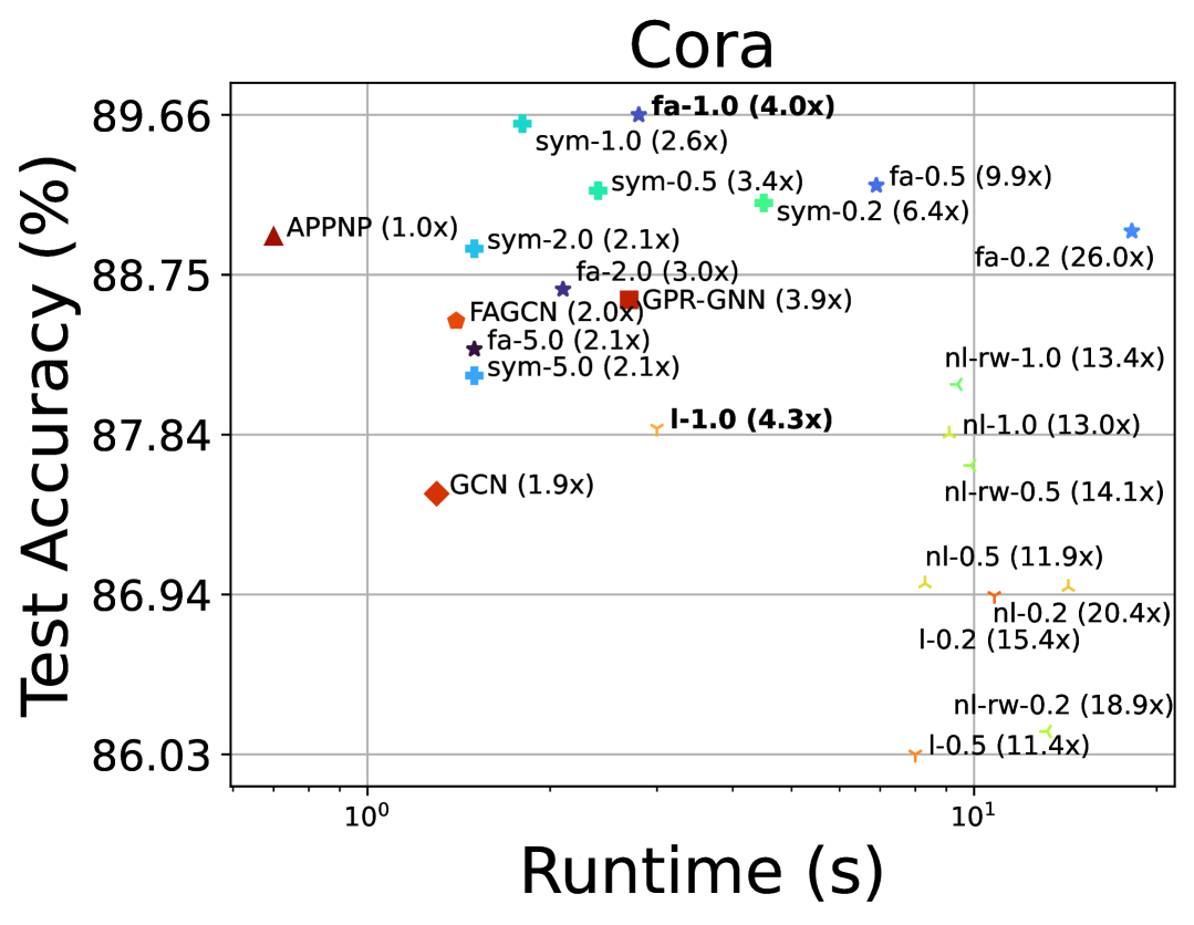
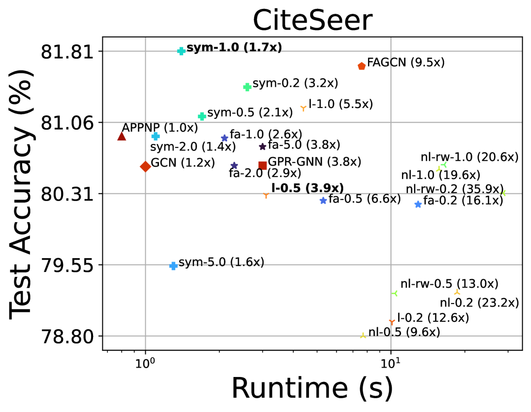
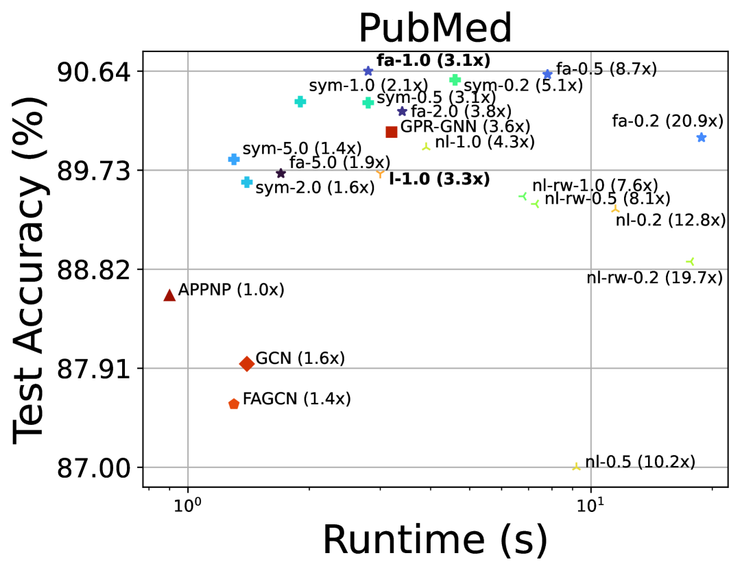
We analyze the efficiency of GWN in Figure 8. We compare GWN at different with four basic GNNs and three variants of GRAND (GRAND-l, GRAND-nl, and GRAND-nl-rw). GWN-sym is faster than GWN-fa because it has fewer learnable parameters. And as increases, their runtime becomes faster. Taking CiteSeer as an example, ”sym-1.0 (1.7x)” achieves both optimal performance and competitive efficiency. Furthermore, GRAND exhibits overall less efficiency, with its three variants mainly cluster on the right side of figures, and their runtimes are on the order of . Considering its most efficient variant ”l-0.5 (3.9x)”, its performance and runtime are still inferior to our variant ”sym-1.0 (1.7x)”. It demonstrates that our models can achieve both efficient and effective performance.
As shown in Table 7 and Table 8, we present the complete performance and efficiency of GWN at different . The results and runtimes for all models are obtained using the optimal parameters. It is important to note that the runtime, in addition to time step , can be affected by parameters such as the number of layers, learning rate, and hidden layer dimensions. Therefore, there are cases where the runtime increases for larger compared to smaller .