2.0cm2.0cm1.0cm1.0cm
On free arrangements of three conics
Abstract
We give a complete classification of free arrangement of three smooth conics on complex projective plane admitting only singularities and singularities.
1 Introduction
The aim of this paper is to classify all free arrangements (up to the projective equivalence) of three smooth conics in admitting only certain quasi-homogeneous singularities. Let us recall that an arrangement of plane curves is called free if its associated module of derivations is a free module over the coordinate ring of the complex projective plane. The free arrangements of conics with quasi-homogeneous singularities were studied before by some authors, see [4, 10, 11], but still our knowledge and understanding of these arrangements is far from being complete, even in a very natural setting of conic arrangements with only singularities. Free curves are not common objects because they are generally difficult to find or construct.
The inspiration for our study of arrangements of three smooth conics is [11, Theorem 2.2] which states that if an arrangement of smooth conics with some simple singularities is free, then . This restriction is, to some extent, surprising and it is very natural to ask whether we can completely classify such arrangements.
It is known that there exists only one (up to the projective equivalence) -parameter family of two smooth conics that is free [3, Proposition 5.5], i.e., every member of this family is free. Additionally, two free arrangements of three smooth conics are also known. One of them is the arrangement with the defining equations
This arrangement is well-known in algebraic geometry and it is called Persson’s triconical arrangement [9]. The other one is the arrangement presented in [11], with three conics defined by the following equations:
We are also aware of examples of free arrangements of four smooth conics, for instance one based on Persson’s triconical arrangement (see [5, Example 3.3]). However, we are not aware of any free arrangements of four smooth conics admitting only singularities of type , , , and (this notation is according to Arnold’s classification of singularities [1]).
Our research project focuses on finding all free arrangements of three and four smooth conics with singularities, and in this article we make the first step into this direction, namely we deliver a classification result on free arrangements of three smooth conics, see Theorem A. Additionally, we show that there are no free arrangements containing a singularity of type , which is a quasi-homogeneous singularity that is not , see Theorem B.
2 Preliminaries
For a projective situation, with a point and a homogeneous polynomial , we take local affine coordinates such that and then the dehomogenization of .
Definition 2.1.
Let be an isolated singularity of a polynomial . Since we can change the local coordinates, let . The number
is called the Milnor number of at .
The number
is called the Tjurina number of at .
Additionally, the total Tjurina number of a given reduced curve is defined as
Let us denote by the coordinate ring of and for a homogeneous polynomial let us denote by the Jacobian ideal associated with . Let be a reduced curve in of degree defined by . Denote by the associated Milnor algebra.
Definition 2.2.
We say that a reduced plane curve is an -syzygy curve when has the following minimal graded free resolution:
with and .
In the setting of the above definition, the minimal degree of the Jacobian relations among the partial derivatives of is defined to be .
Definition 2.3.
We say that is free if and only if , and then .
A useful criterion for studying the freeness of curves is Du Plessis-Wall theorem [7]:
Theorem 2.4.
A reduced plane curve with is free if and only if
| (1) |
We present below the local normal forms of the singularities we are interested in, and these equations are taken from Arnold’s paper [1]. All of these singularities are quasi-homogeneous.
| with | , |
| with | , |
We are going to study arrangements of conics from the perspective of pairs consisting of them. Any arrangement of smooth conics for can be split into pairs. In Table 2, we show all possible configurations of a pair of smooth conics, along with the graph notation captured from[12, Table 2.1]. In the last column, we introduce our own symbolic notation for each pair. We are going to use this notation throughout the paper.
| Graph notation | Picture | Singularities | Symbolic notation | ||
|
|
|
||||
| four | |||||
| (four nodes) | |||||
|
|
|
||||
| one , two | |||||
| (one tacnode, two nodes) | |||||
|
|
|
||||
| two | |||||
| (two tacnodes) | |||||
|
|
|
one , one | |||
|
|
|
one |
Example 2.5.
In this arrangement of three conics, given by
we have two singularities, three singularities and one singularity. This configuration splits into three pairs as follows:
Using the notation from Table 2, we write this decomposition as .
3 Free configurations of three conics with only ADE singularities
Here is the list of all possible ADE singularities in configurations of three smooth plane conics:
-
1.
– node, in which two conics intersect transversally,
-
2.
– tacnode, in which two conics are tangent with multiplicity ,
-
3.
– point in which two conics are tangent with multiplicity ,
-
4.
– point in which two conics are tangent with multiplicity ,
-
5.
– point where three conics intersect pairwise transversally,
-
6.
– two conics and have an singularity and the third conic passes transversally through that singularity,
-
7.
– two conics and have an singularity and the third conic passes transversally through that singularity,
-
8.
– two conics and have an singularity and the third conic passes transversally through that singularity.
Table 3 shows all the notations and values of the Milnor number (which in this case is equal to the Tjurina number) and the multiplicities of all the singularities on this list. The values and the notation from this table will be used in the following sections of the paper.
| Number of | |||
| Singularity | occurrences | Multiplicity | |
| 1 | 1 | ||
| 3 | 2 | ||
| 4 | 3 | ||
| 5 | 3 | ||
| 6 | 4 | ||
| 7 | 4 | ||
| 8 | 5 | ||
| 10 | 6 |
Let us recall some definitions first, based on [11]. Recall that the germ is weighted homogeneous of type with if there are local analytic coordinates centered at and a polynomial with , where the sum is over all pairs with . Using this description, the Arnold exponent (a log canonical threshold) of can be defined as
If is a configuration of three smooth conics with only singularities, then by [6, Theorem 2.1] we know that we have where is the minimum of the Arnold exponents of the singular points of . In the case of a configuration with only singularities, we have (see [2, Corollary 7.45 and inequality 7.46]), so we have . Since for free curves, we have . Therefore by Theorem 2.4 we get . Hence, using the values of and notation from the table above, we obtain the following system of equations:
| (2) |
where the second equation refers to the well-known naive combinatorial counting of the intersections among conics. By finding all solutions of (2) in nonnegative integers, we obtain the following result:
Theorem 3.1.
A configuration of three smooth conics with only singularities is free if and only if it has one of the following weak combinatorics:
Now we introduce some simple lemmas, which we will use later to show that most of these weak combinatorics cannot be realized geometrically over the complex numbers.
Lemma 3.2.
If a configuration of smooth conics with only quasi-homogeneous singularities has singularities of type and singularities of type , then by splitting the configuration into pairs of conics, we obtain pairs of type .
Proof.
This is a straightforward observation resulting from the analysis of the list of singularities in arrangements of smooth conics at the beginning of this section. Namely, a pair of type can only be obtained from an singularity or from a singularity.
Lemma 3.3.
If a configuration of smooth conics with only quasi-homogeneous singularities has singularities of type and singularities of type , then by splitting the configuration into pairs of conics, we obtain pairs of type .
Proof.
Analogous to the proof of Lemma 3.2.
Lemma 3.4.
If a configuration of smooth conics with only quasi-homogeneous singularities has singularities of type and singularities of type , then by splitting the configuration into pairs of conics, we obtain pairs of type and pairs of type , with .
Proof.
This equality is a consequence of counting the singularities.
Lemma 3.5.
If a configuration of smooth conics with only quasi-homogeneous singularities has at least one singularity of type or , then it does not contain singularities of type , or .
Proof.
If a configuration has a or singularity, there exists a pair of conics which intersect only at one point (with multiplicity ). However, a singularity of type , or requires three conics to intersect and each intersection index is smaller than , which is a contradiction.
Lemma 3.6.
If a configuration of smooth conics with only quasi-homogeneous singularities has more than one pair without nodes (i.e. or ), then it does not contain singularities of type , and .
Proof.
In order for the singularity of type , and to exist, there must be two different pairs of conics with singularities. However, if a configuration has more than one pair without nodes, there exists at most one pair with singularities, a contradiction.
Lemma 3.7.
If a configuration of smooth conics with only quasi-homogeneous singularities has at least one singularity of type then each pair of conics has to contain nodes (i.e. , or ).
Proof.
The singularity splits into three pairs, where two pairs have nodes and one pair has the singularity (i.e. ). A pair of type also contains a node.
Proposition 3.8.
The following weak combinatorics:
cannot be realized over by three smooth conics.
Proof.
From Lemmas 3.3 and, 3.4 we obtain at least pairs in the decomposition in each case, which is a contradiction.
Proposition 3.9.
The following weak combinatorics
cannot be realized over by smooth conics.
Proof.
Follows from Lemma 3.5.
Proposition 3.10.
The following weak combinatorics
cannot be realized over by smooth conics.
Proof.
Follows from Lemma 3.6.
Proposition 3.11.
The configuration of three smooth conics with the weak combinatoric
cannot exist.
Proof.
Suppose that such a configuration exists. Then it splits into pairs of type and one pair of type . Since does not contain a node, this weak combinatoric cannot be realized from Lemma 3.7.
Proposition 3.12.
The configuration of three conics with the weak combinatoric
cannot exist.
Proof.
Suppose that such a configuration exists. Then it splits into pairs of type and one pair of type . The singularity is formed by joining the singularity with two nodes. These nodes must come from two pairs. The singularity is formed by joining the singularity with two nodes. Since we already used the nodes from both pairs, the only remaining ones are from the pair, but these two nodes are clearly distinct, a contradiction.
Before we proceed, we introduce the following two facts which will be used in our proofs.
Fact 3.13.
Let and be two distinct smooth conics.
-
a)
If and form the arrangement (i.e. with singularities and ), then the equation of can be written in the form
where , is the equation of a line tangent to at the singularity and is the equation of a line passing through both singularities.
-
b)
If and form the arrangement (i.e. with one singularity and two nodes), then the equation of can be written in the form
where , is the equation of a line tangent to at the singularity and is the equation of a line passing through both nodes.
-
c)
If and form the arrangement (i.e. with two singularities), then the equation of can be written in the form
where and , are the equation of lines tangent to at the respective singularities.
-
d)
If and form the arrangement (i.e. with one singularity), then the equation of can be written in the form
where and is the equation of a line tangent to at the singularity.
Proposition 3.14.
The following weak combinatoric
cannot be realized over by smooth conics.
Proof.
Suppose that there exists a configuration admitting this weak combinatoric. The only possible decomposition into pairs is . Using the method presented in [12] (see Table 2), this configuration of conics can be represented by the following graph.
By [8, Proposition 3], we may assume that
for some , . By [12, Remark 4.3.2] we know that , have following parametrizations:
Let us assume that is given by . Since and intersect in and cannot contain those points, then by parametrizations of and we obtain that the intersection points of with and must be of the form
respectively, where and . By substituting these points into the equation of , we obtain
and
By the intersection behaviour of with and , we have and for some nonzero and . By comparing the coefficients, we obtain the following system of equations:
If , then from (V) we get , but this implies which is a contradiction, hence we know that .
From (I), (VI), we obtain . Then (II) and (VII) implies , which is equivalent to
| (*) |
Now, from (IV) and (IX), we obtain
| (**) |
By adding (I) and (V), we get
| (***) |
Now, after subtracting (I) and (V) we obtain . Similarly, from (II) and (IV) we get
respectively. From (III) we get . Now by substituting it into the (VIII) and using (*), (**) we obtain
Substituting in (III), we get
| (****) |
Now, by (***) and (****) we can find formulas for :
Having determined in terms of and we can express by
which is a contradiction with irreducibility of .
Proposition 3.15.
The following weak combinatoric
cannot be realized over by smooth conics.
Proof.
Suppose that such a configuration of three conics , and exists and it is represented by the following graph:
By [12, Proposition 4.2.1], we may assume that
for some . These two quadrics meet at the point with multiplicity and they have parametrizations
Suppose such a quadric exists. Since , then will meet with at the points and with multiplicities and respectively, where . Similarly, will meet with at the points and with multiplicities , when . In addition, the line is tangent to at and the line passes through the intersection points and . Therefore by Fact 3.13 a) the equation of must be in the form of
for some . Substituting the affine parametrization , , of into the above equation, we obtain
On the other hand, by the intersection behavior of and , must be of the form
Comparing these two equations, we obtain
From the first equations, we obtain
Then, by substituting these equalities into the third equation and simplifying, we finally obtain that , which contradicts our earlier assumption that .
Proposition 3.16.
The following weak combinatoric
cannot be realized over by smooth conics.
Proof.
Suppose that such a configuration of three conics , and exists. It can be split into pairs . Using projective transformations, we can assume that the singularity is in and two singularities are in and . Let be the conic which passes through both singularities. Since it also has to pass through the singularity, it is necessarily given by
for some . The lines tangent to at and are and , respectively. The line passing through both intersection points of and is , while the line passing through both intersection points of and is . Therefore, by Fact 3.13 a), the equations of the remaining conics are:
for some We want conics and to be tangent to each other at two points and one of them is . The tangents to and at this point are
respectively. For these lines to be identical, we need
| (3) |
Moreover, the coordinates of points of intersection of and satisfy
We can use this system of equations to determine the second point of tangency. Note that if , then and we obtain the point , so we may assume . By multiplying equations (I) and (II) by and , respectively, and subtracting them, we get
which by (3) further reduces to
Since we only have one more point of intersection of and besides , the discriminant of the above quadratic equation must be zero. However, by (3) this discriminant is equal to , which is a contradiction since and .
Proposition 3.17.
Any free configuration of three quadrics , , with weak combinatorics
is projectively equivalent to the quadrics
with , and .
The statement and proof of the above theorem was already published in [12], however, the formula presented there contains mistakes. The above formula corrects them.
Proposition 3.18.
Any free configuration of three quadrics , , with weak combinatorics
is projectively equivalent to the quadrics
with and .
Proof.
The decomposition into pairs is . By [12, Proposition 4.2.1] we may assume that
for some . These conics intersect at point and with multiplicities and , respectively (and the second point will become a singularity). These two conics have the following parametrizations:
We can therefore write the coordinates of the remaining two singularities of type as and for some with and .
By Fact 3.13 a), we can write the equation defining as , where , is the equation of a line tangent to at point , and is the equation of a line passing through points and . In this case, is defined by equation and is defined by . We therefore obtain
On the other hand, we can write the equation for in the same way, but this time considering its intersection with , i.e. in the form , where and the lines and are defined similarly as before. In this case, we obtain
and therefore
By comparing the coefficients in both equations, we obtain the following system of equations:
From (IV) we obtain . By substituting that into the remaining equations, we obtain (equations (I) and (V)) and (equations (II) and (III)), which leads to . Finally, from equation (III) we get . By substituting these values into any of the above equations defining , we obtain the equation from the statement of our theorem.
Proposition 3.19.
Any free configuration of three quadrics , , with weak combinatorics
is projectively equivalent to the quadrics
with , .
Proof.
The only possible decomposition into pairs is . We assume that this configuration of three conics , and is represented by the following graph:
We can mimic the proof of Proposition 3.18. We use [12, Proposition 4.2.1] to get the equations of and along with their parametrizations. Then we write the equation for in two ways, using Fact 3.13 a) and b). Then, we compare the coefficients in both equations and as a result we obtain the formulas from the statement of our proposition.
(, ).
Proposition 3.20.
Any free configuration of three quadrics , , with weak combinatorics
is projectively equivalent to the quadrics
with , .
Proof.
The only possible decomposition into pairs is . We assume that this configuration of three conics , and is represented by the following graph:
We can mimic the proof of Proposition 3.18. We use [12, Proposition 4.1.1] to get the equations of and along with their parametrizations. Then we write the equation for in two ways, using Fact 3.13 b) and d). Then, we compare the coefficients in both equations and as a result we obtain the formulas from the statement of our proposition.
Remark 3.21.
In this configuration, two singularities and one singularity are always colinear.
Proof.
It can be shown that the coordinates of two singularities are and , while the coordinates of the singularity can be written in the form . It is easy to check that all these points lie on a line given by .
Proposition 3.22.
Any free configuration of three quadrics , , with weak combinatorics
is projectively equivalent to the quadrics
with , , and additionally .
Proof.
The only possible decomposition into pairs is . One singularity coincides with nodes from two other pairs and becomes the singularity.
We can mimic the proof of Proposition 3.18. We use [12, Proposition 4.2.1] to get the equations of and along with their parametrizations. Then we write the equation for in two ways, using Fact 3.13 a). Then, we compare the coefficients in both equations and as a result we obtain the formulas from the statement of our proposition.
Proposition 3.23.
Any free configuration of three quadrics , , with weak combinatorics
is projectively equivalent to the quadrics
with and .
Proof.
The only possible decomposition into pairs is . We assume that this configuration of three conics , and is represented by the following graph:
We can mimic the proof of Proposition 3.18. We use [12, Proposition 4.1.1] to get the equations of and along with their parametrizations. Then we write the equation for in two ways, using Fact 3.13 a) and b). Then, we compare the coefficients in both equations and as a result we obtain the formulas from the statement of our proposition.
().
It can be checked that all in the above propositions, from Proposition 3.8 to Proposition 3.23, we analyzed all possible weak combinatorics listed in Theorem 3.1. Therefore we can gather all these results and write them down in a single main theorem:
Theorem A.
Every free arrangement of three smooth conics over with only singularities is projectively equivalent to one of the following arrangements:
-
(i)
with , . This arrangement has one singularity and two singularities.
-
-
(ii)
-
,
-
,
-
with , . This arrangement has one singularity and three singularities.
-
-
(iii)
with and . This arrangement has two , two and one singularities.
-
-
(iv)
with . This arrangement has two singularities, one singularity and two singularities.
-
-
(v)
where , and additionally . This arrangement has one , two and one singularity.
-
-
(vi)
where . This arrangement has one , one , one and one singularity.
-
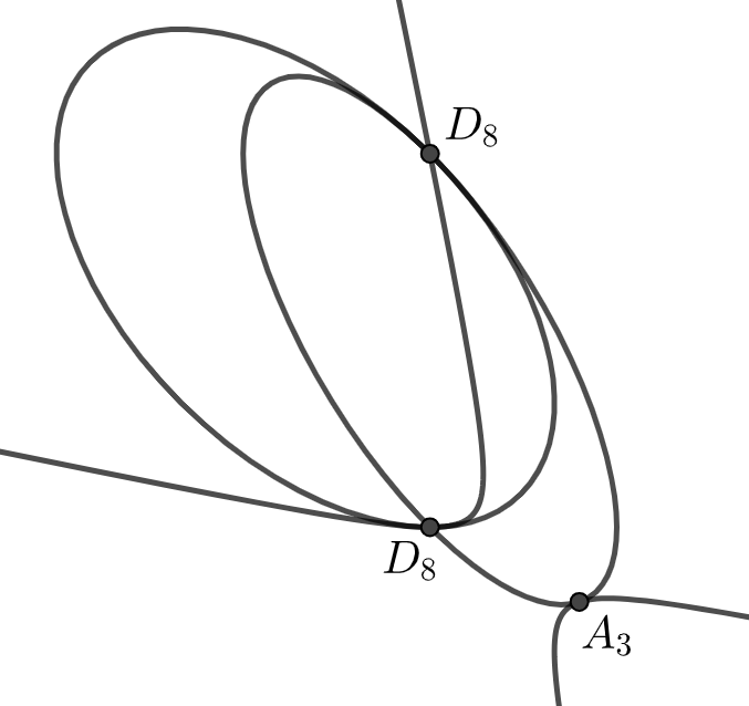
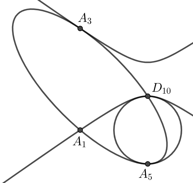
4 Adding the singularity
Given the complete classification of free arrangements of three smooth conics with only singularities, a natural question is to ask how the classification looks when considering all possible quasi-homogeneous singularities. The first step towards the full classification is considering another type of quasi-homogeneous singularity, namely . For this singularity, there are three conics passing through one point such that each pair of conics intersects as an singularity. We present below an appendix to Table 3 with the information about the singularity.
| Number of | |||
| Singularity | occurrences | Multiplicity | |
| 10 | 6 |
By repeating the reasoning from the previous section, we obtain the following system of equations, which is a necessary condition for such free arrangements to exist:
| (4) |
Here, the right side of the first equation comes from Theorem 2.4 for , where the second equation refers to the well-known naive combinatorial counting of the intersections of conics. We have . It turns out that (4) does not have any solutions in non-negative integers when , however we obtain new solutions (apart from the ones from Theorem 3.1) when , so we can write the following result:
Proposition 4.1.
A configuration of three smooth conics with only singularities and at least one singularity is free if and only if it has either one of the weak combinatorics from Theorem 3.1 or one of the following weak combinatorics:
In the following, we will show that none of the above weak combinatorics is realizable over . To begin with, let us write down a useful lemma.
Lemma 4.2.
If a configuration of smooth conics has at least one singularity of type , , or , then it does not contain a singularity of type .
Proof.
Suppose that a configuration of three smooth conics has a singularity at a point and a singularity at a point . Without loss of generality, assume that and intersect at with multiplicity . Then these two conics must also intersect at with multiplicity , which contradicts Bézout’s Theorem. The proof in the remaining cases (, , and ) is analogous.
Proposition 4.3.
The following weak combinatorics
cannot be realized over by smooth conics.
Proof.
Follows from Lemma 4.2.
Proposition 4.4.
The following weak combinatoric
cannot be realized over by smooth conics.
Proof.
Follows from Lemma 3.6.
Proposition 4.5.
The following weak combinatoric
cannot be realized over by smooth conics.
Proof.
Suppose that a configuration realizing this weak combinatoric exists. The only possible decomposition into pairs is . This configuration is represented by the following graph.
By [8, Proposition 3], we may assume that
for some , . These conics intersect in two points: and . Without loss of generality we may assume that is the singularity. By [12, Remark 4.3.2] we know that , have following parametrizations
By Fact 3.13 c) we know that is given by the equation , where and are tangent lines tangent to at two intersection points. We have and from the above parametrization of the second point of intersection is of the form for some , . We therefore have and . In the end we write
Now, consider the intersection of and . Let denote the polynomial in variable obtained by substituting the parametrization of to the above equation of . We have
Since cannot lie in the intersection of and roots of are simply values of that give all the intersection points of and . From the intersection behavior of we also know that must be in the form
We know that the singularity lies in the in the intersection of and therefore we know that which leads to
for some . Thus which implies that the discriminant is equal to . Therefore we can write
Since are all contradictory with our assumptions, the only valid option is . If we substitute into the equation of we get
which is a contradiction with irreducibility of .
As a result from the above propositions, we obtain the second main theorem:
Theorem B.
Every free arrangement of three smooth conics over admitting only singularities and singularities is projectively equivalent to one of the arrangements presented in Theorem A.
References
- [1] V. I. Arnold. Local normal forms of functions. Inventiones mathematicae, 35:87–110, 1976.
- [2] A. Dimca. Topics on Real and Complex Singularities: An Introduction. Advanced Lectures in Mathematics. Vieweg+Teubner Verlag, 2013.
- [3] A. Dimca, G. Ilardi, and G. Sticlaru. Addition-deletion results for the minimal degree of a jacobian syzygy of a union of two curves. Journal of Algebra, 615:77–102, 2023.
- [4] A. Dimca, M. Janasz, and P. Pokora. On plane conic arrangements with nodes and tacnodes. Innov. Incidence Geom., 19(2):47–58, 2022.
- [5] A. Dimca and P. Pokora. Maximizing curves viewed as free curves. International Mathematics Research Notices, 2023(22):19156–19183, 03 2023.
- [6] A. Dimca and E. Sernesi. Syzygies and logarithmic vector fields along plane curves. Journal de l’École polytechnique - Mathématiques, 1:247–267, 2014.
- [7] A. du Plessis and C. Wall. Application of the theory of the discriminant to highly singular plane curves. Mathematical Proceedings of the Cambridge Philosophical Society, 126:259 – 266, 03 1999.
- [8] G. Megyesi. Configurations of conics with many tacnodes. Tohoku Mathematical Journal, 52(4):555 – 577, 2000.
- [9] U. Persson. Horikawa surfaces with maximal picard numbers. Mathematische Annalen, 259:287–312, 1982.
- [10] P. Pokora. -conic arrangements in the complex projective plane. Proc. Amer. Math. Soc., 151(7):2873–2880, 2023.
- [11] P. Pokora. On free and nearly free arrangements of conics admitting certain ADE singularities. Ann. Univ. Ferrara Sez. VII Sci. Mat., 70(3):593–606, 2024.
- [12] C. C. Sarıoğlu. Combinatorics and Topology of Conic Line Arrangement. PhD thesis, Dokuz Eylul University, August 2010. Access: https://acikeris-im.deu.edu.tr/xmlui/bitstream/handle/20.500.12397/9191/283678.pdf.