Kernel Ridge Regression with Predicted Feature Inputs and Applications to Factor-Based Nonparametric Regression

Abstract

Kernel methods, particularly kernel ridge regression (KRR), are time-proven, powerful nonparametric regression techniques known for their rich capacity, analytical simplicity, and computational tractability. The analysis of their predictive performance has received continuous attention for more than two decades. However, in many modern regression problems where the feature inputs used in KRR cannot be directly observed and must instead be inferred from other measurements, the theoretical foundations of KRR remain largely unexplored. In this paper, we introduce a novel approach for analyzing KRR with predicted feature inputs. Our framework is not only essential for handling predicted feature inputs—enabling us to derive risk bounds without imposing any assumptions on the error of the predicted features—but also strengthens existing analyses in the classical setting by allowing arbitrary model misspecification, requiring weaker conditions under the squared loss, particularly allowing both an unbounded response and an unbounded function class, and being flexible enough to accommodate other convex loss functions. We apply our general theory to factor-based nonparametric regression models and establish the minimax optimality of KRR when the feature inputs are predicted using principal component analysis. Our theoretical findings are further corroborated by simulation studies.

Keywords: Reproducing kernel Hilbert space, kernel ridge regression, kernel complexity, nonparametric regression, factor regression model, dimension reduction.

1 Introduction

Regression is one of the most fundamental problems in statistics and machine learning where the goal is to construct a prediction function $f:\mathcal{Z}\to\mathbb{R}$ based on $n$ independent pairs $(Y_{i},Z_{i})\in(\mathbb{R},\mathcal{Z})$, with $1\leq i\leq n$, such that for a new pair $(Y,Z)$, the prediction $f(Z)$ is close to $Y$. Among existing regression approaches, Kernel Ridge Regression (KRR) is a cornerstone of nonparametric regression due to its flexibility, analytical simplicity, and computational efficiency (Kimeldorf and Wahba, 1971; Bach and Jordan, 2002; Steinwart and Christmann, 2008; Cucker and Smale, 2002), making it widely applicable across diverse fields, including finance, bioinformatics, signal processing, image recognition, natural language processing, and climate modeling. In this paper, we study the prediction of KRR when the regression features $Z_{i}$’s are not directly observed and must be predicted from other measurements.

Let $K:{\mathcal{Z}\times\mathcal{Z}}\to\mathbb{R}$ be a pre-specified kernel function. In the classical setting where $n$ pairs of $(Y_{i},Z_{i})$ are observed, KRR searches for the best predictor over the function class $\mathcal{H}_{K}$, the Reproducing Kernel Hilbert Space (RKHS) induced by $K$, by minimizing the penalized least squares loss:

$$\widetilde{f}=\operatorname*{arg\,min}_{f\in\mathcal{H}_{K}}\left\{\frac{1}{n}\sum_{i=1}^{n}\bigl{(}Y_{i}-f(Z_{i})\bigl{)}^{2}+\lambda\|f\|_{K}^{2}\right\}.$$ (1)

Here $\lambda>0$ is some regularization parameter and $\|\cdot\|_{K}$ is the endowed norm of $\mathcal{H}_{K}$. It is well known that the RKHS induced by a universal kernel, such as the Gaussian or Laplacian kernel, is a large function space, as any continuous function can be approximated arbitrarily well by an intermediate function in the RKHS under the infinity norm (Steinwart, 2005; Micchelli et al., 2006). More importantly, the representer theorem (Kimeldorf and Wahba, 1971) ensures that $\widetilde{f}$ in (1) admits a closed-form solution and can be computed effectively. Theoretical properties of $\widetilde{f}$ have been constantly studied over the past two decades, see, for instance, Caponnetto and De Vito (2007); Smale and Zhou (2007); Steinwart and Christmann (2008); Fischer and Steinwart (2020); Cui et al. (2021); Blanchard and Mücke (2018); Rudi and Rosasco (2017), to just name a few.

However, in many modern regression problems across machine learning, natural language processing, healthcare, and finance, the regression features $Z_{1},\ldots,Z_{n}$ in (1) are not directly observed and must be predicted from other measurable features. Consequently, regression such as KRR is performed by regressing the response onto the predicted feature inputs. Below, we present prominent examples, including well-known feature extraction and representation learning techniques in large language models and deep learning.

Example 1 (Dimension reduction via principal component analysis).

KRR, or more broadly, nonparametric regression approaches, are particularly appealing due to their flexibility in approximating any form of the regression function when the feature dimension is small and the sample size is large. However, in many modern applications, the number of features is often comparable to, or even greatly exceeds the sample size. Classical non-parametric approaches including KRR are affected by the curse of dimensionality. To address the high-dimensionality issue, one common approach is to first find a low-dimensional representation of the observed high-dimensional features and then regress the response onto the obtained low-dimensional representation.

Principal Component Analysis (PCA) is the most commonly used method to construct a small number of linear combinations of the original features, known as the Principal Components (PCs) (Hotelling, 1957). The prediction is then made by regressing the response onto the obtained PCs. When this regression step is performed using ordinary least squares, the approach is known as Principal Component Regression (PCR) (Stock and Watson, 2002; Bing et al., 2021; Bai and Ng, 2006; Kelly and Pruitt, 2015), which is fully justified under the following factor-based linear regression model:

$$Y=Z^{\top}\beta+\epsilon,$$ (2)

$$X=AZ+W.$$ (3)

Here both $X\in\mathbb{R}^{p}$ and $Y\in\mathbb{R}$ are observable while $Z\in\mathbb{R}^{r}$, with $r\ll p$, is some unobservable, latent factor. The $p\times r$ loading matrix $A$ is deterministic but unknown, the vector $\beta$ contains the linear coefficients of the factor $Z$, and both $\epsilon\in\mathbb{R}$ and $W\in\mathbb{R}^{p}$ represent additive errors. By centering, we can assume $Y$, $X$ and $Z$ have zero mean. The leading PCs in PCR can be regarded as a linear prediction of the latent factor $Z$. While the linear factor model in (3) is reasonable and widely adopted in the factor model literature (Anderson, 2003; Chamberlain and Rothschild, 1983; Lawley and Maxwell, 1962; Bai, 2003), PCR often yields unsatisfactory predictive performance due to its reliance on linear regression in the low-dimensional space. As a running example of our general theory, we adopt KRR to capture more complex nonlinear relationships between $Y$ and $Z$ in place of (2), while still using (3) to model the dependence between $X$ and $Z$.

Example 2 (Feature extraction via autoencoder).

Unlike PCA, an autoencoder is a powerful alternative in machine learning and data science for constructing a nonlinear low-dimensional representation of high-dimensional features (Goodfellow et al., 2016). Specifically, an autoencoder learns an encoding function $E$ that maps the original features $X\in\mathcal{X}\subseteq\mathbb{R}^{p}$ to its latent representation in $\mathcal{Z}\subseteq\mathbb{R}^{r}$ while simultaneously learning a decoding function $D:\mathcal{Z}\to\mathcal{X}$ to reconstruct the original features from the encoded representation (Bank et al., 2023). Both the encoder and decoder are typically parameterized by using deep neural networks as $E_{\theta}$ and $D_{\vartheta}$, respectively. Given a metric $d:\mathcal{X}\times\mathcal{X}:\to\mathbb{R}^{+}$, for instance, $d(x,x^{\prime})=\|x-x^{\prime}\|_{2}^{2}$ for any $x,x^{\prime}\in\mathcal{X}$, the encoder and decoder are learned by solving the optimization problem:

$$(\widehat{\theta},\widehat{\vartheta}):=\operatorname*{arg\,min}_{\theta,\vartheta}\frac{1}{n}\sum_{i=1}^{n}d\big{(}(D_{\vartheta}\circ E_{\theta})(X_{i}),X_{i}\big{)}.$$

The trained autoencoder provides a method for constructing a low-dimensional representation of the original features, given by $E_{\widehat{\theta}}(X)$, which are then utilized in various downstream supervised learning tasks (Berahmand et al., 2024), with applications found in finance (Bieganowski and Ślepaczuk, 2024), healthcare (Afzali et al., 2024) and climate science (Chen et al., 2023).

Example 3 (Representation learning in large language models).

Recent advancements in natural language processing have demonstrated the effectiveness of large language models (LLMs), such as Transformer-based architectures, in learning meaningful representations of text data (Vaswani et al., 2017; Devlin et al., 2019; Radford et al., 2021). These models convert text input into numerical vector representations, commonly referred to as word embeddings or contextualized embeddings, which capture semantic and syntactic properties of words and phrases.

Formally, a large language model learns an embedding function $E:\mathcal{X}\to\mathcal{Z}$, where $\mathcal{X}$ represents the input text space (e.g., tokenized sequences) and $\mathcal{Z}$ is the latent representation space. This includes the traditional static word embeddings (e.g., Word2Vec or GloVe) where the same token is mapped to a unique representation. Recently, modern transformer-based models produce contextualized embeddings based on the surrounding words. Given a sequence of tokens $X=(x_{1},x_{2},\dots,x_{T})$, a trained transformer model computes the embeddings as:

$$E_{\widehat{\theta}}(X)=\left(E_{\widehat{\theta}}(x_{1}),E_{\widehat{\theta}}(x_{2}),\ldots,E_{\widehat{\theta}}(x_{T})\right),$$

where $E_{\widehat{\theta}}$ denotes the parametrized embedding function, pretrained on large-scale corpora using unsupervised learning objectives, such as masked language modeling (Devlin et al., 2019). The embeddings serve as powerful feature representations for various downstream supervised learning tasks. Let $f_{1}\circ f_{2}$ denote the composition of two functions $f_{1}$ and $f_{2}$. In regression applications, the embeddings of the input text together with their corresponding responses are used to train a regression function $\widehat{f}:\mathcal{Z}\to\mathbb{R}$ with the final predictor given by: $\widehat{f}\circ E_{\widehat{\theta}}:\mathcal{X}\to\mathbb{R}.$ This approach is widely adopted in natural language processing tasks such as sentiment analysis with continuous sentiment scores, automated readability assessment, and financial text-based forecasting, where leveraging pretrained embeddings has been shown to significantly improve prediction performance (Raffel et al., 2020; Brown et al., 2020).

Motivated by the aforementioned examples, in this paper we study the KRR in (1) when the feature inputs $Z_{i}$’s need to be predicted from other measurable features. Concretely, consider $n$ i.i.d. training data $\mathcal{D}=\{(Y_{i},X_{i})\}_{i=1}^{n}\in(\mathbb{R},\mathcal{X})^{n}$ with $\mathcal{X}\subseteq\mathbb{R}^{p}$ and the response $Y_{i}$ generated according to the following non-parametric regression model

$$Y=f^{*}(Z)+\epsilon,$$ (4)

where $Z\in\mathcal{Z}\subseteq\mathbb{R}^{r}$ is some random, unobservable, latent factor with some $r\in\mathbb{N}$, $f^{*}:\mathcal{Z}\to\mathbb{R}$ is the true regression function, and $\epsilon$ is some regression error with zero mean and finite second moment $\sigma^{2}<\infty$. Let $\widehat{g}:\mathcal{X}\to\mathcal{Z}$ be any generic measurable predictor of $Z$ that is constructed independently of $\mathcal{D}$. The KRR predictor $\widehat{f}$ is obtained as in (1) with $Z_{i}$ replaced by its predicted value $\widehat{g}(X_{i})$ for $i\in[n]:=\{1,\ldots,n\}$. The final predictor of KRR using predicted inputs based on $\widehat{g}$ is $\widehat{f}\circ\widehat{g}:\mathcal{X}\to\mathbb{R},$ with its excess risk defined as

$$\mathcal{E}(\widehat{f}\circ\widehat{g})~:=~\mathbb{E}\bigl{[}Y-(\widehat{f}\circ\widehat{g})(X)\bigr{]}^{2}-\sigma^{2}~=~\mathbb{E}\bigl{[}f^{*}(Z)-(\widehat{f}\circ\widehat{g})(X)\bigr{]}^{2},$$ (5)

where $(Y,X)$ is a new random pair following the same model as $\mathcal{D}$. As detailed below, despite existing analyses and results on KRR in the classical setting, little is known about its predictive behavior when feature inputs are subject to prediction errors. In this paper, our goal is to provide a general treatment for analyzing $\mathcal{E}(\widehat{f}\circ\widehat{g})$, which is valid for any generic predictor $\widehat{g}$. The new framework we develop for analyzing KRR is not only indispensable for handling predicted feature inputs but also improves existing analyses in the classical setting by allowing arbitrary model misspecification, requiring weaker conditions under the squared loss, and being flexible enough to accommodate other convex loss functions in (1). We start by reviewing existing approaches for analyzing KRR in the classical setting.

1.1 Existing approaches for analyzing KRR

In the classical setting where the features $Z_{i}$’s in (1) are directly observed, existing techniques for bounding the excess risk of $\widetilde{f}$ under model (4) mainly fall into two streams.

The first proof strategy relies on the integral operator approach (see, e.g., Smale and Zhou (2007); Caponnetto and De Vito (2007); Blanchard and Mücke (2018); Fischer and Steinwart (2020); Rudi and Rosasco (2017), and references therein). Denote by $\rho$ the probability measure of the feature $Z\in\mathcal{Z}$ and by $\mathcal{L}^{2}(\rho)=\{f:\int_{\mathcal{Z}}f^{2}(z)~{\rm d}\rho(z)<\infty\}$ its induced space of square-integrable functions, equipped with the inner product $\langle\cdot,\cdot\rangle_{\rho}$ and norm $\|\cdot\|_{\rho}$. For any $z\in\mathcal{Z}$, by writing $K_{z}:=K(z,\cdot)\in\mathcal{H}_{K}$, the integral operator is $L_{K}:\mathcal{L}^{2}(\rho)\to\mathcal{L}^{2}(\rho)$, defined as

$$L_{K}:f\mapsto\int_{\mathcal{Z}}K_{z}f(z)~{\rm d}\rho(z).$$

Let $\{\mu_{j}\}_{j\geq 1}$ be the eigenvalues of $L_{K}$ and $\{\phi_{j}\}_{j\geq 1}$ be the corresponding eigenfunctions, assuming their existence. When the regression function $f^{*}$ belongs to $\mathcal{H}_{K}$ and the eigenvalues $\mu_{j}$’s satisfy the following polynomial decay condition

$$cj^{-1/\alpha}\leq\mu_{j}\leq Cj^{-1/\alpha},\qquad\text{for all $j\geq 1$ and some $\alpha\in(0,1)$},$$ (6)

Caponnetto and De Vito (2007) established the minimax optimal rate of $\|\widetilde{f}-f^{*}\|_{\rho}^{2}$, which depends on the decaying rate $\alpha$. While the integral operator approach allows for sharp rate analysis of KRR, it oftentimes has limitations in handling model misspecification, and the required conditions on $\mu_{j}$’s could be difficult to verify. Without assuming (6), Smale and Zhou (2007) derives upper bounds of $\|\widetilde{f}-f^{*}\|_{\rho}^{2}$ but their analysis still requires $f^{*}\in\mathcal{H}_{K}$ along with some additional smoothness condition on $f^{*}$. Allowing $f^{*}\notin\mathcal{H}_{K}$ is addressed by Rudi and Rosasco (2017) in the context of learning with random features where the authors resort to a so-called effective dimension condition $\sum_{j}\mu_{j}/(\mu_{j}+\delta)\leq C\delta^{-\alpha}$, for all $\delta>0$ and some $\alpha\in[0,1]$, which is related to but weaker than (6). Alternatively, Fischer and Steinwart (2020); Zhang et al. (2023) handle $f^{*}\notin\mathcal{H}_{K}$ by relying on the smoothness condition $f^{*}=L_{K}^{r}g^{*}$ for some $g^{*}\in\mathcal{L}^{2}(\rho)$ and some $r\in(0,1/2]$ as well as the upper bound requirement in condition (6).

The other proof strategy for analyzing KRR adopts the empirical risk minimization perspective and employs probabilistic tools from empirical process theory to establish excess risk bounds. See, e.g., Bartlett et al. (2005); Mendelson and Neeman (2010); Steinwart et al. (2009); more recently, Ma et al. (2023); Duan et al. (2024), and references therein. Inherited from the classical learning theory, this proof strategy has the potential to deal with model misspecification and can be easily applied to KRR in (1) in which the squared loss is replaced by other convex loss functions (Eberts and Steinwart, 2013). However, the existing works typically assume boundedness conditions on the response variable and the function class, or restrictive conditions on the eigen-decomposition of $L_{K}$. For instance, the analyses in Mendelson and Neeman (2010); Ma et al. (2023); Duan et al. (2024) require the eigenfunctions $\{\phi_{j}\}_{j\geq 1}$ of $L_{K}$ to be uniformly bounded, a useful condition for obtaining improved $\|\cdot\|_{\infty}$ bound but is not always satisfied even for the most popular kernel functions (Zhou, 2002). On the other hand, the authors of Bartlett et al. (2005) derive prediction risk bounds for general empirical risk minimization based on local Rademacher complexity, and applied them to analyze $\widetilde{f}_{bd}$, which is computed from (1) with $\lambda=0$ but constrained to the unit ball $\mathcal{B}_{\mathcal{H}}:=\{f:\|f\|_{K}\leq 1\}$. A key step in their proof is connecting the local Rademacher complexity of $\mathcal{B}_{\mathcal{H}}$ with the kernel complexity function

$$R(\delta)=\biggl{(}{1\over n}\sum_{j=1}^{\infty}\min\{\delta,\mu_{j}\}\biggr{)}^{1/2},\qquad\forall~\delta\geq 0,$$

using the result proved in Mendelson (2002). The kernel complexity function depends not only on $\mathcal{H}_{K}$ but also on the probability measure $\rho$ of $Z$ through the integral operator $L_{K}$, and is commonly used to characterize the complexity of $\mathcal{H}_{K}$. Indeed, it is closely related with the effective dimension (Caponnetto and De Vito, 2007; Rudi and Rosasco, 2017), covering numbers (Cucker and Smale, 2002) and related capacity measures (Steinwart and Christmann, 2008). Let $\delta_{n}>0$ be the fixed point of $R(\delta)$ such that $R(\delta_{n})=\delta_{n}$. The risk bound of $\widetilde{f}_{bd}$ in Bartlett et al. (2005) reads

$$\mathbb{P}\left\{\|\widetilde{f}_{bd}-f^{*}\|_{\rho}^{2}~\lesssim~\delta_{n}+{t\over n}\right\}\geq 1-e^{-t},\qquad\forall~t\geq 0.$$ (7)

However, the analysis of Bartlett et al. (2005) requires the response variable $Y$ and $\mathcal{H}_{K}$ to be bounded, as well as $f^{*}\in\mathcal{H}_{K}$. The case $f^{*}\notin\mathcal{H}_{K}$ is considered in Steinwart et al. (2009) where the authors derive an oracle inequality for the prediction risk of a truncated version of the KRR predictor $\widetilde{f}$. But their analysis requires $Y$ to be bounded, condition (6) and the approximation error to satisfy $\inf_{f\in\mathcal{H}_{K}}\{\|f^{*}-f\|_{\rho}^{2}+\lambda\|f\|_{K}^{2}\}\leq C\lambda^{\beta}$ for some $\beta\in(0,1]$ and $\lambda>0$. The last requirement turns out be related to the aforementioned smoothness condition $f^{*}=L_{K}^{r}g^{*}$ with $r\in(0,1/2]$.

Summarizing, even in the classical setting where the feature inputs are observed, existing analyses of KRR require either that the true regression function belongs to the specified RKHS, that both the RKHS and the response $Y$ are bounded, or that certain conditions on the eigenvalues or eigenfunctions of the RKHS hold. As explained in the next section, our new framework of analyzing KRR removes such restrictions under the squared loss in (1), while remaining applicable to the analysis of general convex loss functions.

More substantially, when the feature inputs $Z_{i}$ in (1) must be predicted by $\widehat{g}(X_{i})$, neither of the above two proof strategies can be applied. This is because both the integral operator $L_{K}$ and the kernel complexity function $R(\delta)$, defined via the eigenvalues of $L_{K}$, depend on the probability measure $\rho$ of the latent feature $Z$. When regressing $Y$ onto the predicted feature $\widehat{g}(X)$, following either strategy would lead to a different integral operator $L_{x,K}$ and a different kernel complexity function, both of which depend on the probability measure $\rho_{x}$ of $\widehat{g}(X)$. Let $\{\mu_{x,j}\}_{j\geq 1}$ be the eigenvalues of $L_{x,K}$. The new kernel complexity function is

$$R_{x}(\delta)=\biggl{(}{1\over n}\sum_{j=1}^{\infty}\min\{\delta,\mu_{x,j}\}\biggr{)}^{1/2},\qquad\forall~\delta\geq 0.$$

Establishing a direct relationship between either $R_{x}(\delta)$ and $R(\delta)$, or between $\{\mu_{j}\}_{j\geq 1}$ and $\{\mu_{x,j}\}_{j\geq 1}$, however, is generally intractable without imposing strong assumptions on the relationship between $\rho_{x}$ and $\rho$. Handling predicted feature inputs thus requires a new proof strategy.

1.2 Our contributions

We summarize our main contributions in this section.

1.2.1 Non-asymptotic excess risk bounds of KRR with predicted feature inputs

Our first contribution is to establish new non-asymptotic upper bounds on the excess risk of the KRR predictor $\widehat{f}\circ\widehat{g}$. In particular, our risk bounds are valid for any generic predictor $\widehat{g}$ without imposing any assumptions on the proximity of $\widehat{g}(X)$ to $Z$. Moreover, our results allow arbitrary model misspecification and do not require either the response or the RKHS to be bounded.

To allow for model misspecification, we assume in 1 of Section 3.1 only the existence of $f_{\mathcal{H}}\in\mathcal{H}_{K}$, which is the $\mathcal{L}^{2}(\rho)$ projection of $f^{*}$ onto $\mathcal{H}_{K}$. Using $f_{\mathcal{H}}$, the excess risk of $\widehat{f}\circ\widehat{g}$ is decomposed in (3.1) of Section 3.1 as

$$\mathcal{E}(\widehat{f}\circ\widehat{g})~\lesssim~\mathbb{E}[\ell_{\widehat{f}\circ\widehat{g}}(Y,X)]+\mathbb{E}\Delta_{\widehat{g}}+\|f_{\mathcal{H}}-f^{*}\|_{\rho}^{2}$$ (8)

where $\|f_{\mathcal{H}}-f^{*}\|_{\rho}^{2}$ represents the approximation error, $\Delta_{\widehat{g}}:=\|K_{Z}-K_{\widehat{g}(X)}\|_{K}^{2}$ reflects the error of predicting $Z$ by $\widehat{g}(X)$ through the kernel function $K$, and

$$\ell_{\widehat{f}\circ\widehat{g}}(y,x):=\bigl{(}y-(\widehat{f}\circ\widehat{g})(x)\bigr{)}^{2}-\bigl{(}y-(f_{\mathcal{H}}\circ\widehat{g})(x)\bigr{)}^{2}$$

denotes the squared loss of $\widehat{f}\circ\widehat{g}$ relative to $f_{\mathcal{H}}\circ\widehat{g}$. Analyzing the term $\mathbb{E}[\ell_{\widehat{f}\circ\widehat{g}}(Y,X)]$ in (8) turns out to be the main technical challenge, and its bound also depends on both $\mathbb{E}\Delta_{\widehat{g}}$ and $\|f_{\mathcal{H}}-f^{*}\|_{\rho}^{2}$. In Theorem 2 of Section 3.2, we stated our main result:

Theorem 1 (Informal).

For any $\eta\in(0,1)$ and a suitable choice of $\lambda$ in (1), with probability $1-\eta$, one has

$$\mathcal{E}(\widehat{f}\circ\widehat{g})~\lesssim~\delta_{n}\log(1/\eta)+\mathbb{E}\Delta_{\widehat{g}}+\|f_{\mathcal{H}}-f^{*}\|_{\rho}^{2}+\frac{\log(1/\eta)}{n}.$$ (9)

Theorem 1 holds for any predictor $\widehat{g}$ of $Z$ that is constructed independently of $\mathcal{D}$ and any $f^{*}\in\mathcal{L}^{2}(\rho)$. In particular, it does not impose any restrictions on $\mathbb{E}\Delta_{\widehat{g}}$, the prediction error for $Z$, nor on the approximation error $\|f_{\mathcal{H}}-f^{*}\|_{\rho}^{2}$. Regardless of their magnitudes, both terms appear additively in the risk bound, a particular surprising result for $\mathbb{E}\Delta_{\widehat{g}}$. This is a new result to the best of our knowledge. Even in the classical setting, the rate in (9) with $\mathbb{E}\Delta_{\widehat{g}}=0$ generalizes the existing result in (7) by allowing arbitrary model misspecification, as well as unboundedness of both the response and the RKHS. Moreover, even when the model is correctly specified, our analysis achieves the same optimal rate without imposing any regularity or decaying conditions on $\mu_{j}$’s, such as those in (6), in contrast to existing integral operator approaches, for instance, Fischer and Steinwart (2020); Steinwart et al. (2009); Caponnetto and De Vito (2007); Rudi and Rosasco (2017).

In Section 3.2.1 we further derive more transparent expression of $\mathbb{E}\Delta_{\widehat{g}}$. For the kernel function $K$ that satisfies a Lipschitz property (see, 5), $\mathbb{E}\Delta_{\widehat{g}}$ can be simplified to $\mathbb{E}\|\widehat{g}(X)-Z\|^{2}_{2}$, the $\mathcal{L}^{2}$ prediction error of $\widehat{g}(X)$. To discuss the order of $\delta_{n}$ in (9), we present in Section 3.2.2 its slow rate in Corollary 1 and its fast rates under three common classes of kernel functions: linear kernels in Corollary 2, kernels with polynomially decaying eigenvalues in Corollary 3, and kernels with exponentially decaying eigenvalues in Corollary 4. Our new risk bounds generalize existing results in all cases by characterizing the dependence on both the approximation error and the error in predicting the feature inputs.

In Section 5, we further extend our analysis to other convex loss functions in (1) that satisfy some classical smoothness and strong convexity conditions.

1.2.2 A new framework for analyzing KRR with predicted feature inputs

Along with our new rate results comes a novel approach to analyzing the KRR with predicted inputs. The framework we develop offers two key contributions: (1) it improves existing analyses of KRR in the classical setting by accommodating arbitrary model misspecification and allowing both an unbounded response and an unbounded RKHS; (2) it is essential for handling predicted feature inputs, enabling us to derive risk bounds without imposing any assumptions on the proximity of $\widehat{g}(X)$ to $Z$.

To accomplish the first point, we adopt a hybrid approach that combines the integral operator method with the local Rademacher complexity based empirical process theory from Bartlett et al. (2005), along with a careful reduction argument. This is necessary because the integral operator approach cannot easily handle model misspecification, while the empirical process theory requires both a bounded response and a bounded RKHS. Specifically, as seen in the decomposition (8), the key is to bound from above $\mathbb{E}[\ell_{\widehat{f}\circ\widehat{g}}(Y,X)]$. Since $\sup_{f\in\mathcal{H}_{K}}\|f\|_{K}$ could be unbounded, we first apply a reduction argument, showing that bounding $\mathbb{E}[\ell_{\widehat{f}\circ\widehat{g}}(Y,X)]$ can be reduced to controlling the empirical process

$$\sup_{f\in\uline{\mathcal{F}_{b}}}\Bigl{\{}\mathbb{E}[\ell_{f\circ\widehat{g}}(Y,X)]-2\mathbb{E}_{n}[\ell_{f\circ\widehat{g}}(Y,X)]\Bigr{\}}$$ (10)

where $\uline{\mathcal{F}_{b}}$ is a bounded subset of $\mathcal{H}_{K}$, given by (37) of Section 3.4. We use $\mathbb{E}_{n}$ in this paper to denote the expectation with respect to the empirical measure of $n$ i.i.d. samples. To further address the unboundedness of $Y$, we need to bound the cross-term $\mathbb{E}_{n}[\epsilon(f\circ\widehat{g})(X)-\epsilon(f_{\mathcal{H}}\circ\widehat{g})(X)]$ uniformly over $f\in\uline{\mathcal{F}_{b}}$. To accomplish this, we employ both the empirical process theory based on local Rademacher complexity from Bartlett et al. (2005) and the integral operator approach, as detailed in Section B.2.3; see also Lemma 7. Our analysis only requires moment conditions on the regression error $\epsilon$. Finally, the local Rademacher complexity technique from Bartlett et al. (2005) is applied once again to control the remaining bounded components in the empirical process (10). Due to our new hybrid approach, the analysis can be easily applied to learning algorithms in (1) in which other convex loss functions are used in place of the squared loss, as demonstrated in Section 5.

Another fundamental difficulty in our analysis arises from handling predicted feature inputs. As noted in the end of Section 1.1, the primary challenge lies in establishing a precise connection between the local Rademacher complexity and the kernel complexity function $R(\delta)$ in the presence of errors in predicting the features. The existing analysis in Mendelson (2002) only establishes a connection to $R_{x}(\delta)$, which depends on the probability measure $\rho_{x}$ of $\widehat{g}(X)$. And it is hopeless to relate $R_{x}(\delta)$ with $R(\delta)$ without imposing restrictive assumptions on the closeness of $\rho_{x}$ and $\rho$. To circumvent this issue, rather than working with the population-level local Rademacher complexity and $R_{x}(\delta)$—both of which rely on $\rho_{x}$—we instead focus on their empirical counterparts. The first step is to relate the local Rademacher complexity to its empirical counterpart where we borrow existing concentration inequalities of local Rademacher complexities in Boucheron et al. (2000, 2003); Bartlett et al. (2005). By adapting the argument in Bartlett et al. (2005, Lemma 6.6), we further link the empirical local Rademacher complexity to $\widehat{R}_{x}(\delta)$, the empirical counterpart of $R_{x}(\delta)$. The next step is to connect $\widehat{R}_{x}(\delta)$ to $\widehat{R}(\delta)$, with the latter being the empirical counterpart of $R(\delta)$. This is the most challenging step, as $\widehat{R}_{x}(\delta)$ and $\widehat{R}(\delta)$ depend, respectively, on the empirical integral operators associated with $\widehat{g}(X_{i})$ and $Z_{i}$ for $i\in[n]$. Our proof reveals that this requires to control the spectral difference between two $n\times n$ kernel matrices with entries equal to $K(\widehat{g}(X_{i}),\widehat{g}(X_{j}))$ and $K(Z_{i},Z_{j})$ for $i,j\in[n]$. As accomplished in Lemmas 11 and 12 of Section B.3.3, this is highly non-trivial as we do not impose any requirements on the proximity of $\widehat{g}(X_{i})$ to $Z_{i}$. Finally, we establish sharp concentration inequalities between $\widehat{R}(\delta)$ and its population-level counterpart, $R(\delta)$, to close the loop of relating the local Rademacher complexity to $R(\delta)$. Completing the loop requires a series of technical lemmas, collected in Lemmas 9, 10, 11, 12, and 13 of Sections B.3.1, B.3.2, B.3.3 and B.3.4. Developing this proof strategy is part of our contribution, and we provide a more detailed discussion in Section 3.4.3. For illustration, Figure 1 below depicts how we relate the local Rademacher complexity to the kernel complexity $R(\delta)$, represented by the solid arrow.

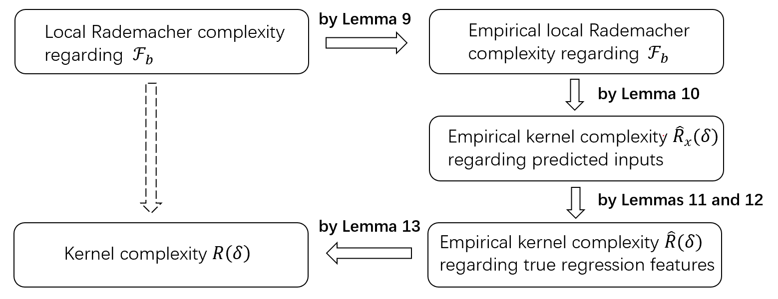
Figure 1: Proof strategy of relating local Rademacher complexity to kernel complexity $R(\delta)$.

1.2.3 Application to factor-based non-parametric regression models

Our third contribution is to provide a complete analysis of using KRR with feature inputs predicted by PCA under the factor-based nonparametric regression models (3) and (4). As an application of our general theory, together with the existing literature on high-dimensional factor models (for instance, Bai (2003); Fan et al. (2013)), we state in Corollary 5 of Section 4.2 an explicit upper bound of the excess risk of the KRR with inputs predicted by PCA. Furthermore, in Theorem 3 of Section 4.2, we establish a matching minimax lower bound of the excess risk under models (3) and (4), thereby demonstrating the minimax optimality of the KRR using the leading PCs.

Prediction consistency of Principal Component Regression (PCR) has been established in Stock and Watson (2002) under the factor-based linear regression models (2) and (3). Explicit rates of the excess risk are later given in Bing et al. (2021), where a general linear predictor of $X_{i}$, including PCA as a particular instance, is used to predict $Z_{i}$. In a more recent work (Fan and Gu, 2024), the authors investigate the predictive performance of fitting neural networks between the response and the retained PCs, proving minimax optimal risk bounds under the factor model (3) when the regression function belongs to a hierarchical composition of functions in the Hölder class. Under model (3) and (4) with $f^{*}$ belonging to some RKHS, our results in Section 4 provide the first minimax optimal risk bound for using KRR with the leading PCs. Moreover, our theory extends beyond the factor model (3), as it applies to any predictor $\widehat{g}$ of $Z$ and accommodates arbitrary dependence between $X$ and $Z$.

This paper is organized as follows: we introduce the learning algorithm of KRR with predicted inputs in Section 2. Theoretical results of analyzing KRR with predicted inputs are stated in Section 3. The risk decomposition is given in Section 3.1 while the risk bounds along with the main assumptions are stated in Section 3.2. Risk bounds for specific kernels are given in Section 3.3 while in Section 3.4 we explain the proof sketch and highlight the main technical difficulties. In Section 4 we apply our general result to factor-based nonparametric regression models. In Section 5 we extend our analysis and derive risk bounds for general convex loss functions. Simulation studies are stated in Appendix A and all proofs are deferred to the Appendix.

Notation. For any $a,b\in\mathbb{R}$, we write $a\wedge b=\min\{a,b\}$ and $a\vee b=\max\{a,b\}$. For any integer $d$, we let $[d]=\{1,\ldots,d\}$. For any symmetric, semi-positive definite matrix $Q\in\mathbb{R}^{d\times d}$, we use $\lambda_{1}(Q)\geq\lambda_{1}(Q)\geq\ldots\geq\lambda_{d}(Q)$ to denote its eigenvalues. For any matrix $A$, we use $\|A\|_{\rm op}$ and $\|A\|_{\text{F}}=(\sum A^{2}_{ij})^{1/2}$ to denote its operator norm and Frobenius norm, respectively. We use $\mathbf{I}_{d}$ to denote the $d\times d$ identity matrix. For $d_{1}\geq d_{2}$, we write $\mathbb{O}_{d_{1}\times d_{2}}$ for matrices with orthonormal columns. The inner product and the endowed norm in the Euclidean space are denoted as $\langle\cdot,\cdot\rangle_{2}$ and $\|\cdot\|_{2}$, respectively. For any function $f:\mathcal{Z}\to\mathbb{R}$, $\|f\|_{\infty}=\sup_{z\in\mathcal{Z}}|f(z)|$. For any two sequences $a_{n}$ and $b_{n}$, we write $a_{n}\lesssim b_{n}$ if there exists some constant $C$ such that $a_{n}\leq Cb_{n}$ for all $n$. We write $a_{n}\asymp b_{n}$ if $a_{n}\lesssim b_{n}$ and $b_{n}\lesssim a_{n}$. In this paper, we use $c,c^{\prime},C$ and $C^{\prime}$ to denote constants whose values may vary line by line unless otherwise stated.

2 Kernel ridge regression with predicted feature inputs

In this section, we state the learning algorithm for Kernel Ridge Regression (KRR) with predicted feature inputs. Recall that $\mathcal{D}=\{(Y_{i},X_{i})\}_{i=1}^{n}\in(\mathbb{R},\mathcal{X})^{n}$ contains $n$ training data. Let $\widehat{g}:\mathcal{X}\to\mathcal{Z}$ be any measurable function that is used to predict the features $Z_{i}\in\mathcal{Z}$. For instance, $\widehat{g}$ could be obtained from one of the feature extraction or representation learning approaches mentioned in the Introduction. The predicted feature inputs are $\widehat{g}(X_{i})$ for all $i\in[n]$.

Let $K:{\mathcal{Z}\times\mathcal{Z}}\to\mathbb{R}$ be some pre-specified kernel function and denote by $\mathcal{H}_{K}$ the Reproducing Kernel Hilbert Space (RKHS) induced by $K$. Write the equipped inner product in $\mathcal{H}_{K}$ as $\langle\cdot,\cdot\rangle_{K}$ and the endowed norm as $\|\cdot\|_{K}$. For any $v\in\mathcal{Z}$, by writing $K_{v}:=K(v,\cdot)\in\mathcal{H}_{K}$, the reproducing property asserts that

$$\langle f,K_{v}\rangle_{K}=f(v),\qquad\forall~f\in\mathcal{H}_{K}.$$ (11)

Equipped with $\mathcal{H}_{K}$, we adopt KRR by regressing the response $\mathbf{Y}=(Y_{1},\ldots,Y_{n})^{\top}$ onto the predicted inputs $\widehat{g}(X_{1}),\ldots,\widehat{g}(X_{n})$ by solving the following optimization problem:

$$\widehat{f}=\operatorname*{arg\,min}_{f\in\mathcal{H}_{K}}\left\{\frac{1}{n}\sum_{i=1}^{n}\bigl{(}Y_{i}-(f\circ\widehat{g})(X_{i})\bigl{)}^{2}+\lambda\|f\|_{K}^{2}\right\}.$$ (12)

Thanks to the reproducing property in (11), the representer theorem (Kimeldorf and Wahba, 1971) states that the minimization in (12) admits a closed-form solution:

$$\widehat{f}=\frac{1}{\sqrt{n}}\sum_{i=1}^{n}\widehat{\alpha}_{i}K_{\widehat{g}(X_{i})}$$ (13)

where the representer coefficients $\widehat{\alpha}=(\widehat{\alpha}_{1},\ldots,\widehat{\alpha}_{n})^{\top}$ are obtained by

$$\widehat{\alpha} =\operatorname*{arg\,min}_{\alpha\in\mathbb{R}^{n}}\left\{{1\over n}\bigl{\|}\mathbf{Y}-\sqrt{n}~\mathbf{K}_{x}\alpha\bigr{\|}_{2}^{2}+\lambda~\alpha^{\top}\mathbf{K}_{x}\alpha\right\}={1\over\sqrt{n}}\bigl{(}\mathbf{K}_{x}+\lambda\mathbf{I}_{n}\bigr{)}^{-1}\mathbf{Y}.$$ (14)

Here $\mathbf{K}_{x}$ is the $n\times n$ kernel matrix with entries equal to $n^{-1}K(\widehat{g}(X_{i}),\widehat{g}(X_{j}))$ for $i,j\in[n]$. Finally, for a new data point $X\in\mathcal{X}$, we predict its corresponding response $Y$ by

$$(\widehat{f}\circ\widehat{g})(X)=\frac{1}{\sqrt{n}}\sum_{i=1}^{n}\widehat{\alpha}_{i}K\left(\widehat{g}(X_{i}),\widehat{g}(X)\right).$$ (15)

Remark 1 (Independence between $\widehat{g}$ and $\mathcal{D}$).

Our theory in Section 3 requires that $\widehat{g}$ be constructed independently of the training data $\mathcal{D}$. This independence simplifies our analysis, especially given the technical complexity of the current framework. Moreover, such independence can lead to better results in many statistical problems, including smaller prediction or estimation errors and weaker conditions – a phenomenon has been observed in various problems, such as estimating the optimal instrument in sparse high-dimensional instrumental variable models (Belloni et al., 2012), inferring a low-dimensional parameter in the presence of high-dimensional nuisance parameters (Chernozhukov et al., 2018), and performing discriminant analysis using a few retained principal components of high-dimensional features (Bing and Wegkamp, 2023). On the other hand, in many applications such as the examples mentioned in the Introduction, auxiliary data without labels or responses are readily available or at least easy to obtain (Bengio et al., 2013). When this is not the case, one can still use a procedure called $k$-fold cross-fitting (Chernozhukov et al., 2018). The 2-fold version of this method first splits the data into equal parts, computes $\widehat{g}$ on one subset, and then performs the regression step using the other subset, before switching their roles. The final prediction is then made by the average of the two resulting predictors.

3 Theoretical guarantees of KRR with predicted feature inputs

In this section we present our theoretical guarantees of the KRR estimator $\widehat{f}$ in (12) that is based on a generic predictor $\widehat{g}:\mathcal{X}\to\mathcal{Z}$, constructed independently of $\mathcal{D}$. The quantity of our interest is the excess risk of the prediction function $\widehat{f}\circ\widehat{g}:~\mathcal{X}\to\mathbb{R}$, given by

$$\mathcal{E}\bigl{(}\widehat{f}\circ\widehat{g}\bigr{)}:=\mathbb{E}\bigl{[}Y-(\widehat{f}\circ\widehat{g})(X)\bigr{]}^{2}-\sigma^{2}.$$ (16)

Henceforth, the expectation $\mathbb{E}$ is taken with respect to a new pair $(Y,X)$ that is independent of, and generated from the same model as, the training data $\mathcal{D}$. Since $\mathcal{E}(\widehat{f}\circ\widehat{g})$ is a random quantity depending on $\mathcal{D}$ and $\widehat{g}$, our goal is to establish its rate of convergence in probability. We start by decomposing the excess risk into three interpretable terms.

3.1 Decomposition of the excess risk

For any deterministic $f\in\mathcal{L}^{2}(\rho)$, we proved in Section B.1 that

$$\mathcal{E}\bigl{(}\widehat{f}\circ\widehat{g}\bigr{)}=\mathbb{E}\bigl{[}(Y-(\widehat{f}\circ\widehat{g})(X))^{2}-(Y-(f\circ\widehat{g})(X))^{2}\bigr{]}+\mathbb{E}\left[f^{*}(Z)-(f\circ\widehat{g})(X)\right]^{2}.$$ (17)

To specify the choice of $f$, we make the following blanket assumption. Recall that $\|\cdot\|_{\rho}$ is the induced norm of $\mathcal{L}^{2}(\rho)$.

Assumption 1.

There exists some $f_{\mathcal{H}}\in\mathcal{H}_{K}$ such that $\|f_{\mathcal{H}}-f^{*}\|_{\rho}^{2}=\inf_{f\in\mathcal{H}_{K}}\|f-f^{*}\|_{\rho}^{2}.$

We do not assume $f^{*}\in\mathcal{H}_{K}$ but rather the weaker 1. If the former holds, we immediately have $f_{\mathcal{H}}=f^{*}$. Since $\mathcal{H}_{K}$ is convex, existence of $f_{\mathcal{H}}$ also ensures its uniqueness (Cucker and Smale, 2002). As discussed in Rudi and Rosasco (2017), existence of $f_{\mathcal{H}}$ can be ensured if $\mathcal{H}_{K}$ in 1 is replaced by $\{f\in\mathcal{H}_{K}:\|f\|_{K}\leq R\}$ for any finite radius $R>0$. Alternatively, we can choose $f_{\mathcal{H},\lambda}=\operatorname*{arg\,min}_{f\in\mathcal{H}_{K}}\{\|f-f^{*}\|_{\rho}^{2}+\lambda\|f\|_{K}^{2}\}$ which, for $\lambda>0$, is always unique and exists (Cucker and Smale, 2002). Notably, our results presented below can be applied to any function $f\in\mathcal{H}_{K}$ in replace of $f_{\mathcal{H}}$, including these mentioned examples.

By choosing $f=f_{\mathcal{H}}$ in (17), the second term on the right-hand side (RHS) of (17) represents the irreducible error from two different sources. To see this, by introducing

$$\Delta_{\widehat{g}}:=\|K_{Z}-K_{\widehat{g}(X)}\|_{K}^{2},$$ (18)

we have that for any $\theta\geq 1$, the elementary inequality $(a+b)^{2}\leq xa^{2}+b^{2}/x$ for $x>0$,

$$\mathbb{E}\left[f^{*}(Z)-(f_{\mathcal{H}}\circ\widehat{g})(X)\right]^{2} ~\leq~(1+\theta)~\mathbb{E}\left[f_{\mathcal{H}}(Z)-(f_{\mathcal{H}}\circ\widehat{g})(X)\right]^{2}+{1+\theta\over\theta}\|f_{\mathcal{H}}-f^{*}\|_{\rho}^{2}$$

$$~=~(1+\theta)~\mathbb{E}\left\langle f_{\mathcal{H}},K_{Z}-K_{\widehat{g}(X)}\right\rangle_{K}^{2}+{1+\theta\over\theta}\|f_{\mathcal{H}}-f^{*}\|_{\rho}^{2}$$ by (11)

$$~\leq~(1+\theta)\|f_{\mathcal{H}}\|_{K}^{2}~\mathbb{E}\Delta_{\widehat{g}}+{1+\theta\over\theta}\|f_{\mathcal{H}}-f^{*}\|_{\rho}^{2}.$$ (19)

The last step uses the Cauchy-Schwarz inequality. The quantity $\mathbb{E}\Delta_{\widehat{g}}$ is referred to as the kernel-related latent error, representing the error in using $\widehat{g}(X)$ to predict the latent factor $Z$, composited with the kernel function $K$. The term $\|f_{\mathcal{H}}-f^{*}\|_{\rho}^{2}$ on the other hand represents the approximation error due to model misspecification when $f^{*}\notin\mathcal{H}_{K}$. We provide detailed discussion on both terms after stating our main result in Theorem 2 below. Going back to the risk decomposition in (17), the remaining term with $f_{\mathcal{H}}$ in place of $f$, $\mathbb{E}[(Y-(\widehat{f}\circ\widehat{g})(X))^{2}-(Y-(f_{\mathcal{H}}\circ\widehat{g})(X))^{2}]$, represents the prediction risk of $\widehat{f}\circ\widehat{g}$ relative to $f_{\mathcal{H}}\circ\widehat{g}$. Analyzing this term is the main challenge in our analysis, and is detailed in the next section.

3.2 Non-asymptotic upper bounds of the excess risk

In this section we establish non-asymptotic upper bounds of the excess risk $\mathcal{E}(\widehat{f}\circ\widehat{g})$ in (16). An important component of our analysis is the empirical process theory based on local Rademacher complexities developed in Bartlett et al. (2005), building on a line of previous works such as Koltchinskii and Panchenko (2000); Bousquet et al. (2002); Massart (2000); Lugosi and Wegkamp (2004). In our context, local Rademacher complexities translate into the complexity of the RKHS. We begin with a brief review of the basics of RKHS, followed by a discussion of its complexity measures and the assumptions used in our analysis.

In this paper, we make the following assumption on the kernel function. It is satisfied by many widely used kernel functions including the Gaussian and Laplacian kernels.

Assumption 2.

The kernel function $K$ is continuous, symmetric and positive semi-definite. Moreover, there exists some positive constant $\kappa<\infty$ such that $\sup_{z,{z}^{\prime}\in\mathcal{Z}}K(z,{z}^{\prime})\leq\kappa^{2}$.

A key element for analyzing $\widehat{f}$ in (12) is the integral operator $L_{K}:\mathcal{L}^{2}(\rho)\to\mathcal{L}^{2}(\rho)$, defined as

$$L_{K}f:=\int_{\mathcal{Z}}K_{z}f(z)~{\rm d}\rho(z).$$ (20)

Our next condition assumes that the integral operator $L_{K}$ can be eigen-decomposed.

Assumption 3.

There exist a sequence of eigenvalues $\{\mu_{j}\}_{j=1}^{\infty}$ arranged in non-increasing order and corresponding eigenfunctions $\{\phi_{j}\}_{j=1}^{\infty}$ that form an orthonormal basis of $\mathcal{L}^{2}(\rho)$, such that $L_{K}=\sum_{j=1}^{\infty}\mu_{j}\langle\phi_{j},\cdot\rangle_{\rho}~\phi_{j}.$

3 is common in the literature of kernel methods. It is guaranteed, for instance, by the celebrated Mercer’s theorem (Mercer, 1909) when the domain of the kernel function $K$ is compact together with 2, although it can also hold in more general settings (see, e.g., Wainwright (2019, Theorem 12.20)).

Under Assumption 3, the kernel function $K$ admits

$$K(z,{z}^{\prime})=\sum_{j=1}^{\infty}\mu_{j}\phi_{j}(z)\phi_{j}({z}^{\prime}),\qquad\forall~z,z^{\prime}\in\mathcal{Z}.$$ (21)

In the case $\mu_{j}>0$ for all $j\geq 1$, the RKHS can be explicitly written as

$$\mathcal{H}_{K}=\Bigg{\{}f=\sum_{j=1}^{\infty}\gamma_{j}\phi_{j}:\ \sum_{j=1}^{\infty}\frac{\gamma_{j}^{2}}{\mu_{j}}<\infty\Bigg{\}}.$$

For any $f_{1}=\sum_{j=1}^{\infty}\alpha_{j}\phi_{j}$ with $\alpha_{j}=\langle f_{1},\phi_{j}\rangle_{\rho}$ and $f_{2}=\sum_{j=1}^{\infty}\beta_{j}\phi_{j}$ with $\beta_{j}=\langle f_{2},\phi_{j}\rangle_{\rho}$, the equipped inner product of $\mathcal{H}_{K}$ is

$$\langle f_{1},f_{2}\rangle_{K}=\sum_{j=1}^{\infty}\frac{\alpha_{j}\beta_{j}}{\mu_{j}}.$$

If for some $k\in\mathbb{N}$, $\mu_{j}>0$ for $j\leq k$ and $\mu_{j}=0$ for all $j>k$, the RKHS reduces to a $k$-dimensional function space spanned by $\{\phi_{1},\ldots,\phi_{k}\}$. In the rest of this paper, we are only interested in non-degenerate kernels, that is, $\mu_{1}>0$.

In classical literature of learning theory, the risk bounds are determined by the richness of the function class. Classical measures include the Vapnik–Chervonenkis dimension (Vapnik and Chervonenkis, 2015), metric entropy (Pollard, 2012) and (local) Rademacher complexity (Koltchinskii and Panchenko, 2000; Koltchinskii, 2001; Mendelson, 2002; Bartlett et al., 2005), see also the references therein. In our case the function class is $\mathcal{H}_{K}$, and its complexity is commonly measured by the following kernel complexity function based on the eigenvalues of the integral operator $L_{K}$,

$$R(\delta)=\biggl{(}\frac{1}{n}\sum_{j=1}^{\infty}\min\left\{\delta,{\mu}_{j}\right\}\biggr{)}^{1/2},\qquad\forall\ \delta\geq 0.$$ (22)

As detailed in Section 3.4, the (local) Rademacher complexity turns out to be closely related with $R(\delta)$ (Mendelson, 2002). An important quantity in our excess risk bounds is the critical radius $\delta_{n}$, defined as the fixed point to $R(\delta)$, i.e., the positive solution to

$$R(\delta)=\delta.$$ (23)

It can be verified that $R(\delta)$ is a sub-root function of $\delta$, so that both existence and uniqueness of its fixed point $\delta_{n}$ are guaranteed (Bartlett et al., 2005, Lemma 3.2). Here we recall that

Definition 1.

A function $\psi:[0,\infty)\to[0,\infty)$ is called sub-root if it is non-decreasing, and if $\delta\mapsto\psi(\delta)/\sqrt{\delta}$ is non-increasing for $\delta>0$.

More basic properties of sub-root functions are reviewed in Section C.1.

Finally, we assume the regression error in model (4) to have sub-Gaussian tails. This simplifies our analysis and can be relaxed to sub-exponential tails or bounded finite moments.

Assumption 4.

There exists some constant $\gamma_{\epsilon}<\infty$ such that $\mathbb{E}[\exp(t\epsilon)]\leq\exp(t^{2}\gamma_{\epsilon}^{2})$ for all $t\in\mathbb{R}$.

The following theorem is our main result which provides non-asymptotic upper bounds of the excess risk of $\widehat{f}\circ\widehat{g}$, given in (16).

Theorem 2.

Grant model (4) and Assumptions 1–4. For any $\eta\in(0,1)$, by choosing $\lambda$ in (12) such that

$$\lambda=C\left(\delta_{n}\log(1/\eta)+\mathbb{E}\Delta_{\widehat{g}}+\|f_{\mathcal{H}}-f^{*}\|_{\rho}^{2}+\frac{\log(1/\eta)}{n}\right),$$ (24)

with probability at least $1-\eta$, one has

$$\mathcal{E}(\widehat{f}\circ\widehat{g})~\leq~C^{\prime}\left(\delta_{n}\log(1/\eta)+\mathbb{E}\Delta_{\widehat{g}}+\|f_{\mathcal{H}}-f^{*}\|_{\rho}^{2}+\frac{\log(1/\eta)}{n}\right).$$ (25)

Here both positive constants $C$ and $C^{\prime}$ depend only on $\kappa$, $\|f^{*}\|_{\infty}$, $\|f_{\mathcal{H}}\|_{K}$ and $\gamma_{\epsilon}^{2}$.

The explicit dependence of $C$ and $C^{\prime}$ on $\kappa$, $\|f^{*}\|_{\infty}$, $\|f_{\mathcal{H}}\|_{K}$ and $\gamma_{\epsilon}^{2}$ can be found in the proof. Since the proof of Theorem 2 is rather long, we defer its full statement to Section B.2. In Section 3.4 we offer a proof sketch and highlight the main technical difficulties.

As shown in Theorem 2, the excess risk is essentially determined by the critical radius $\delta_{n}$, the kernel-related latent error $\mathbb{E}\Delta_{\widehat{g}}$ and the approximation error $\|f_{\mathcal{H}}-f^{*}\|_{\rho}^{2}$. We discuss each term in detail shortly. It is worth emphasizing that Theorem 2 does not impose any assumptions on the magnitudes of either $\mathbb{E}\Delta_{\widehat{g}}$ or $\|f_{\mathcal{H}}-f^{*}\|_{\rho}^{2}$. Surprisingly, regardless of the magnitude of $\mathbb{E}\Delta_{\widehat{g}}$, it appears additively in the risk bound.

Remark 2 (Comparison with the existing theory of KRR in the classical setting).

Although Theorem 2 is derived for the case where the feature inputs are predicted, it is insightful to compare it with the existing results of KRR in the classical setting. When $Z_{1},\ldots,Z_{n}$ are directly observed and used in (1), setting $\mathbb{E}\Delta_{\widehat{g}}=0$ with $\widehat{g}(z)=z$ for $z\in\mathcal{Z}$ simplifies the risk bound (25) to

$$\mathcal{E}(\widehat{f}\circ\widehat{g})~\lesssim~\delta_{n}\log(1/\eta)+\frac{\log(1/\eta)}{n}+\|f_{\mathcal{H}}-f^{*}\|_{\rho}^{2}$$ (26)

which, to the best of our knowledge, is also new in the literature of kernel learning methods. As mentioned in Section 1.1, most existing analyses of KRR cannot handle arbitrary model misspecification without requiring regularity and decay properties of the eigenvalues $\mu_{j}$’s. When the model is correctly specified, our risk bound in (26) matches that in (7), derived by Bartlett et al. (2005). However, their analysis requires both the response variable and the RKHS to be bounded, which we do not assume. Compared to the integral operator approach, our analysis does not impose any restrictive conditions on the eigenvalues $\mu_{j}$’s, which are often required in the existing literature (Caponnetto and De Vito, 2007; Lin and Zhou, 2018; Steinwart et al., 2009; Fischer and Steinwart, 2020). For instance, Caponnetto and De Vito (2007); Rudi and Rosasco (2017) require $\mu_{1}\geq\lambda$ in their analysis, a condition that is somewhat counterintuitive. Such refinement of our result stems from a distinct proof strategy, contributing to a new analytical framework for kernel-based learning. We provide in Section 3.4 further discussion on technical details.

Remark 3 (Discussion on the approximation error).

If we choose the kernel $K$ using some universal kernels, such as the Gaussian kernel or Laplacian kernel, it is known that the induced RKHS is dense in the space of bounded continuous functions ${\cal C}(\cal Z)$ under the infinity norm (Micchelli et al., 2006). If we further assume $f^{*}\in{\cal C}(\mathcal{Z})$, then $\|f_{\mathcal{H}}-f^{*}\|_{\rho}=0$ for universal kernels. Indeed, for any $\vartheta>0$, there must exist some $f_{\vartheta}\in{\cal H}_{K}$ such that $\|f_{\vartheta}-f^{*}\|_{\infty}\leq\vartheta$. This implies that

$$\|f_{\mathcal{H}}-f^{*}\|_{\rho}\leq\|f_{\vartheta}-f^{*}\|_{\rho}\leq\|f_{\vartheta}-f^{*}\|_{\infty}\leq\vartheta.$$

The leftmost inequality uses the definition of $f_{\mathcal{H}}$ in 1.

3.2.1 Discussion on the kernel-related latent error

Recall from (18) that the term $\mathbb{E}\Delta_{\widehat{g}}$ reflects the error of $\widehat{g}(X)$ in predicting $Z$ through the kernel function $K$. To obtain more transparent expression, we need the following Lipschitz property of the map $\mathcal{Z}\to\mathcal{H}_{K}$, that is, $z\mapsto K_{z}$ for all $z\in\mathcal{Z}$.

Assumption 5.

There exists some positive constant $C_{K}$ such that

$$\bigl{\|}K_{z}-K_{z^{\prime}}\bigr{\|}_{K}\leq C_{K}\|z-z^{\prime}\|_{2},\qquad\forall\ z,z^{\prime}\in\mathcal{Z}.$$

5 can be verified for various kernels. One sufficient condition is the following uniform boundedness condition of the mixing partial derivatives of the kernel function (Blanchard et al., 2011): there exists some constant $C>0$ such that

$$\sup_{z,z^{\prime}\in\mathcal{Z}}\left\|\frac{\partial^{2}K(z,z^{\prime})}{\partial z\partial z^{\prime}}\right\|_{{\rm op}}\leq~C.$$ (27)

Condition (27) holds for several commonly used kernels, such as the linear kernel and the Gaussian kernel (Blanchard and Zadorozhnyi, 2019; Sun et al., 2022).

Under 5, the kernel-related latent error can be bounded by

$$\mathbb{E}\Delta_{\widehat{g}}~\leq~C_{K}^{2}~\mathbb{E}\|\widehat{g}(X)-Z\|_{2}^{2},$$ (28)

entailing consistent prediction of $Z$ itself by using $\widehat{g}(X)$. We remark that this can be relaxed when the kernel function $K$ is invariant to orthogonal transformations, that is, $K(z,z^{\prime})=K(Qz,Qz^{\prime})$ for any $z,z^{\prime}\in\mathcal{Z}$ and any $Q\in\mathbb{O}_{r\times r}$. When this is the case, we only need consistent prediction of $Z$ up to an orthogonal transformation, in the precise sense that

$$\mathbb{E}\Delta_{\widehat{g}}~\leq~C_{K}^{2}\inf_{Q\in\mathbb{O}_{r\times r}}\mathbb{E}\|\widehat{g}(X)-QZ\|_{2}^{2}.$$ (29)

This claim is proved in Section B.4. We give below two common classes of kernel functions that are invariant to orthogonal transformations. Let $h:\mathbb{R}\to\mathbb{R}$ be some kernel-specific function.

• Inner product kernel: $K(z,z^{\prime})=h(\langle z,z^{\prime}\rangle_{2})$, e.g. linear kernels, polynomial kernels;

• Radial basis kernel: $K(z,z^{\prime})=h(\|z-z^{\prime}\|_{2})$, e.g. exponential kernels, Gaussian kernels.

3.2.2 Discussion on the critical radius

The critical radius $\delta_{n}$ defined in (23) is an important factor in the risk bound (25). Finding its exact expression is difficult in general. To quantify its rate of convergence, by the sub-root property of $R(\delta)$ and 2, we prove in Section B.5 the following slow rate of $\delta_{n}$:

$$\delta_{n}~\leq~{\kappa/\sqrt{n}}.$$ (30)

Together with Theorem 2, we have the following slow rate of convergence of the excess risk.

Corollary 1 (Slow rate of the excess risk).

Grant model (4) and Assumptions 1–5. For any $\eta\in(0,1)$ with $\log(1/\eta)\leq\sqrt{n}$, by choosing $\lambda$ as in (24) with $\delta_{n}$ replaced by $\kappa/\sqrt{n}$, with probability at least $1-\eta$, one has

$$\mathcal{E}(\widehat{f}\circ\widehat{g})~\leq~C^{\prime}\left(\frac{\log(1/\eta)}{\sqrt{n}}+\mathbb{E}\|\widehat{g}(X)-Z\|_{2}^{2}+\|f_{\mathcal{H}}-f^{*}\|_{\rho}^{2}\right).$$ (31)

Here the positive constant $C^{\prime}$ depends only on $\kappa$, $\|f^{*}\|_{\infty}$, $\|f_{\mathcal{H}}\|_{K}$, $\gamma_{\epsilon}^{2}$ and $C_{K}$.

The first $n^{-1/2}$-type rate is well-known in the literature of kernel methods when $Z_{1},\ldots,Z_{n}$ are observed and no assumptions on the smoothness of $f^{*}\in\mathcal{H}_{K}$ or decaying properties of the eigenvalues $\mu_{j}$’s are made. See, for instance, Corollary 5 in Smale and Zhou (2007) and Caponnetto and De Vito (2007). Our new result additionally accounts for both the model misspecification and the error due to predicting feature inputs.

In many situations, however, fast rates of $\delta_{n}$ are obtainable, as we discuss below. For ease of presentation, assume $f_{\mathcal{H}}=f^{*}$ for now. To explain the role of $\delta_{n}$, we follow Yang et al. (2017) by introducing the concept of statistical dimension, which is defined as the last index for which the kernel eigenvalues $\{\mu_{j}\}_{j\geq 1}$ exceed $\delta_{n}$, that is,

$$d(\delta_{n})=\max\left\{j\geq 0:{\mu}_{j}\geq\delta_{n}\right\}$$

with $\mu_{0}:=\infty$. In view of the expression of $R(\delta)$ in (22), this implies

$$\delta_{n}=R(\delta_{n})=\biggl{(}{d(\delta_{n})\over n}~\delta_{n}+{1\over n}\sum_{j>d(\delta_{n})}\mu_{j}\biggr{)}^{1/2}.$$

If $\sum_{j>d(\delta_{n})}\mu_{j}\lesssim d(\delta_{n})\delta_{n}$ holds, we can conclude that $\delta_{n}\asymp{d(\delta_{n})/n}$, hence the name statistical dimension for $d(\delta_{n})$. Any kernel whose eigenvalues satisfy this condition is said to be regular (Yang et al., 2017). More importantly, for any regular kernel, Yang et al. (2017, Theorem 1) shows that in the fixed design setting ($Z_{i}$’s are treated as deterministic), an empirical version of $\delta_{n}$ serves as a fundamental lower bound on the in-sample prediction risk of any estimator:

$$\inf_{f}\sup_{\|f^{*}\|_{K}\leq 1}\mathbb{E}_{n}[f(Z)-f^{*}(Z)]^{2}~\gtrsim~\widehat{\delta}_{n}$$

where the infimum is taken over all estimators based on $\{Y_{i},Z_{i}\}_{i=1}^{n}$, and $\widehat{\delta}_{n}$ is the positive solution to $\widehat{R}(\delta)=\delta$ with $\widehat{R}(\delta)$ being the empirical kernel complexity function, given in (44). In the random design settings, we prove in Theorem 3 that $\widehat{\delta}_{n}$ in the lower bound is indeed replaced by $\delta_{n}$. In the next section we derive explicit expressions of $\delta_{n}$ for some specific kernels.

3.3 Explicit excess risk bounds for specific kernel classes

To establish explicit rates of $\delta_{n}$, we consider three common classes of kernels, including the linear kernels, kernels with polynomially decaying eigenvalues and kernels with exponentially decaying eigenvalues. We also present simplified excess risk bounds of Theorem 2 for each class. For ease of presentation, we assume $f_{\mathcal{H}}=f^{*}$ and $\kappa=1$ in the rest of this section.

3.3.1 Linear kernels

Consider $\mathcal{Z}\subseteq\mathbb{R}^{r}$ for some $r\in\mathbb{N}$. We start with the linear kernel

$$K(z,{z}^{\prime})=z^{\top}{z}^{\prime},\qquad\forall~z,z^{\prime}\in\mathcal{Z}.$$

Denote by $\Sigma_{Z}$ the second moment matrix of $Z$ and write its eigen-decomposition as $\Sigma_{Z}=\sum_{j=1}^{r}\sigma_{j}v_{j}v_{j}^{\top}$ where the eigenvalues are arranged in non-increasing order. For simplicity, we assume ${\rm rank}(\Sigma_{Z})=r$ whence the induced $\mathcal{H}_{K}$ also has rank $r$. For each $j\in[r]$, define $\phi_{j}:\mathcal{Z}\to\mathbb{R}$ as

$$\phi_{j}(z):=\sigma_{j}^{-1/2}v_{j}^{\top}z,\qquad\forall~z\in\mathcal{Z}.$$

It is easy to verify that

$$K(z,z^{\prime})=z^{\top}z^{\prime}=z^{\top}\sum_{j=1}^{r}v_{j}v_{j}^{\top}z^{\prime}=\sum_{j=1}^{r}\sigma_{j}\phi_{j}(z)\phi_{j}(z^{\prime}),\qquad\forall\ z,z^{\prime}\in\mathcal{Z}.$$ (32)

The following corollary states the simplified excess risk bound of Theorem 2 for the linear kernel. Its proof is deferred to Section B.6. The notation $\lesssim_{\eta}$ denotes the inequality holds up to $\log(1/\eta)$.

Corollary 2.

Consider the linear kernel. Grant model (4) with $f^{*}\in\mathcal{H}_{K}$ and Assumptions 1–5. For any $\eta\in(0,1)$, with probability at least $1-\eta$, one has

$$\mathcal{E}(\widehat{f}\circ\widehat{g})~\lesssim_{\eta}~\frac{r}{n}+\mathbb{E}\|\widehat{g}(X)-Z\|_{2}^{2}.$$ (33)

The term $r/n$ is as expected for the prediction risk under linear regression models using $\{(Y_{i},Z_{i})\}_{i=1}^{n}$. Note that it only depends on the dimension of the latent factor $Z$ instead of the ambient dimension of $X$. The second term, $\mathbb{E}\|\widehat{g}(X)-Z\|_{2}^{2}$, represents the error in using $\widehat{g}(X)$ to predict $Z$. When $\widehat{g}$ is chosen as PCA (see Section 4.2 for details), the predictor $\widehat{f}\circ\widehat{g}$ coincides with the Principal Component Regression (PCR). Our risk bound aligns with existing works of PCR (Stock and Watson, 2002; Bing et al., 2021), although it holds for more general predictor $\widehat{g}$.

3.3.2 Kernels with polynomially decaying eigenvalues

We consider the kernel class satisfying the $\alpha$-polynomial decay condition in their eigenvalues, that is, there exists some $\alpha>1/2$ and some absolute constant $C>0$ such that ${\mu}_{j}\leq Cj^{-2\alpha}$ for all $j\geq 1$. Several widely used kernels, including the Sobolev kernel and the Laplacian kernel, belong to this class. See, Chapters 12 and 13 in Wainwright (2019), for more examples. The quantity $\alpha$ controls the complexity of $\mathcal{H}_{K}$, with a smaller $\alpha$ indicating a more complex $\mathcal{H}_{K}$.

The following corollary states simplified risk bounds of Theorem 2 for such kernels with polynomially decaying eigenvalues. Its proof can be found in Section B.7.

Corollary 3.

Consider the polynomial decay kernels. Grant model (4) with $f^{*}\in\mathcal{H}_{K}$ and Assumptions 1–5. For any $\eta\in(0,1)$, the following holds with probability at least $1-\eta$,

$$\mathcal{E}(\widehat{f}\circ\widehat{g})~\lesssim_{\eta}~n^{-\frac{2\alpha}{2\alpha+1}}+\mathbb{E}\|\widehat{g}(X)-Z\|_{2}^{2}.$$ (34)

The first term in the risk bound (34) corresponds to the minimax optimal prediction risk established in Caponnetto and De Vito (2007) when $n$ i.i.d. pairs of $(Y_{i},Z_{i})$ are observed. As $\alpha$ decreases and the corresponding $\mathcal{H}_{K}$ becomes more complex, the first term decays more slowly, while the term $\mathbb{E}\|\widehat{g}(X)-Z\|_{2}^{2}$ becomes easier to absorb into the first term.

An important example of an RKHS induced by polynomial decay kernels is the well-known Sobolev RKHS. Specifically, consider the case where $\mathcal{Z}\subset\mathbb{R}^{r}$ is open and bounded, and $\rho$ has a density with respect to the uniform distribution on $\mathcal{Z}$ (Steinwart et al., 2009). For any integer $s>r/2$, let $W_{s}(\mathcal{Z})$ denote the Sobolev space of smoothness $s$. When $s=r=1$, the Sobolev space $W_{1}(\mathcal{Z})$ is an RKHS induced by $K(z,z^{\prime})=\min\{z,z^{\prime}\}$. For more general settings, we refer the reader to Novak et al. (2018) for the explicit form of the kernel function that induces $W_{s}(\mathcal{Z})$. As described by Edmunds and Triebel (1996, Equation 4 on page 119), the eigenvalues $\{\mu_{j}\}_{j\geq 1}$ corresponding to $W_{s}(\mathcal{Z})$ satisfy the polynomial decay condition with $\alpha=s/r>1/2$. As a result, the excess risk bound in Corollary 3 becomes

$$\mathcal{E}(\widehat{f}\circ\widehat{g})~\lesssim_{\eta}~n^{-\frac{2s}{2s+r}}+\mathbb{E}\|\widehat{g}(X)-Z\|_{2}^{2}.$$

The first term follows the classical nonparametric rate but depends only on $r$, the dimension of the latent factor $Z$, rather than the ambient dimension of $\mathcal{X}$. It tends to zero as long as $r=o(\log n)$ for any fixed smoothness $s$. By contrast, when applying KRR directly to predict the response from $X_{1},\ldots,X_{n}\in\mathcal{X}\subseteq\mathbb{R}^{p}$, the excess risk bound would be $n^{-\frac{2s}{2s+p}}$, which does not vanish once $\log n=\mathcal{O}(p)$. When $r\ll p$, reducing to a lower dimension before applying KRR could lead to a significant advantage for prediction. See a concrete example in Section 4.

3.3.3 Kernels with exponentially decaying eigenvalues

We consider in this section RKHSs induced by kernels whose eigenvalues exhibit exponential decay, that is, there exists some $\gamma>0$ such that $\mu_{j}\leq\exp(-\gamma j)$ for all $j\geq 1$. It is well known that the eigenvalues of the Gaussian kernel satisfy this exponential decay condition.

The following corollary states the simplified risk bounds of Theorem 2 for such kernels with exponentially decaying eigenvalues. Its proof can be found in Section B.8.

Corollary 4.

Consider the exponential decay kernels. Grant model (4) with $f^{*}\in\mathcal{H}_{K}$ and Assumptions 1–5. For any $\eta\in(0,1)$, the following holds with probability at least $1-\eta$,

$$\mathcal{E}(\widehat{f}\circ\widehat{g})~\lesssim_{\eta}~\frac{\log n}{n}+\mathbb{E}\|\widehat{g}(X)-Z\|_{2}^{2}.$$ (35)

The first term in the bound of (35) coincides with the minimax optimal rate in the classical setting for an exponentially decaying kernel (see, for instance, Example 2 in Yang et al. (2017) under the fixed design setting). It is interesting to note that absorbing the error from predicting feature inputs into the first term requires a higher accuracy of $\widehat{g}(X)$ in predicting $Z$ for exponentially decaying kernels compared to polynomially decaying kernels.

3.4 Proof techniques of Theorem 2

In this section, we provide a proof sketch of Theorem 2 and highlight its main challenges. The proof consists of three main components, which are discussed separately in the following subsections.

3.4.1 Bounding the empirical process with a reduction argument

Recall that the excess loss function of $f\circ\widehat{g}$ relative to $f_{\mathcal{H}}\circ\widehat{g}$ is:

$$\ell_{f\circ\widehat{g}}(y,x):=\bigl{(}y-(f\circ\widehat{g})(x)\bigr{)}^{2}-\bigl{(}y-(f_{\mathcal{H}}\circ\widehat{g})(x)\bigr{)}^{2},\qquad\forall~x\in\mathcal{X},y\in\mathbb{R}.$$

The first component of our proof employs a delicate reduction argument, showing that proving Theorem 2 can be reduced to bounding from above the empirical process

$$\sup_{f\in\uline{\mathcal{F}_{b}}}\Bigl{\{}\mathbb{E}[\ell_{f\circ\widehat{g}}(Y,X)]-2\mathbb{E}_{n}[\ell_{f\circ\widehat{g}}(Y,X)]\Bigr{\}}$$ (36)

where $\mathbb{E}_{n}$ denotes the expectation with respect to the empirical measure, and $\uline{\mathcal{F}_{b}}$ is the local RKHS-ball around $f_{\mathcal{H}}$, given by

$$\uline{\mathcal{F}_{b}}:=\left\{f\in\mathcal{F}_{b}:\mathbb{E}[\ell_{f\circ\widehat{g}}(Y,X)]\leq\lambda\right\},\qquad\mathcal{F}_{b}:=\left\{f\in\mathcal{H}_{K}:\|f-f_{\mathcal{H}}\|_{K}\leq 3\|f_{\mathcal{H}}\|_{K}\right\}$$ (37)

with $\lambda$ given in (24). Since $\uline{\mathcal{F}_{b}}\subseteq\mathcal{F}_{b}$ and $\mathcal{F}_{b}$ is a bounded function class, which can be seen from

$$\|f\|_{\infty}\leq 4\kappa\|f_{\mathcal{H}}\|_{K},\qquad\forall~f\in\mathcal{F}_{b},$$

by the reproducing property, this reduction argument allows us later to apply existing empirical process theory which is only applicable for bounded function classes. Moreover, the reduction argument ensures that our bound in Theorem 2 depends only on $\|f_{\mathcal{H}}\|_{K}^{2}$, a finite quantity that can be much smaller than $\sup_{f\in\mathcal{H}_{K}}\|f\|_{K}^{2}$, which could be infinite.

The second part of this component is to bound from above the empirical process (36). Since the response variable $Y$ is not assumed to be bounded, existing empirical process theory for bounded functions cannot be directly applied. Instead we rewrite the excess loss function as

$$\mathbb{E}[\ell_{f\circ\widehat{g}}(Y,X)]=\mathbb{E}\left[\bigl{(}f^{*}(Z)-(f\circ\widehat{g})(X)\bigr{)}^{2}-\bigl{(}f^{*}(Z)-(f_{\mathcal{H}}\circ\widehat{g})(X)\bigr{)}^{2}\right]=:\mathbb{E}\left[h_{f\circ\widehat{g}}(Z,X)\right]$$

for the function $h_{f\circ\widehat{g}}:\mathcal{Z}\times\mathcal{X}\to\mathbb{R}$. Also note that its empirical version satisfies

$$\mathbb{E}_{n}[\ell_{f\circ\widehat{g}}(Y,X)]=\mathbb{E}_{n}\left[h_{f\circ\widehat{g}}(Z,X)\right]+2\mathbb{E}_{n}\bigl{[}\epsilon(f_{\mathcal{H}}\circ\widehat{g})(X)-\epsilon(f\circ\widehat{g})(X)\bigr{]}.$$

Our proof in this step relies on the local Rademacher complexity, defined as: for any $\delta\geq 0$,

$$\psi_{x}(\delta):={\mathcal{R}_{n}}\left\{f\circ\widehat{g}-f_{\mathcal{H}}\circ\widehat{g}:f\in\mathcal{F}_{b},~\mathbb{E}\left[(f\circ\widehat{g})(X)-(f_{\mathcal{H}}\circ\widehat{g})(X)\right]^{2}\leq\delta\right\}.$$ (38)

The detailed definition of ${\mathcal{R}_{n}}$ can be found in Section B.2.1. Let $\delta_{x}$ be the fixed point of $\psi_{x}$ such that $\psi_{x}(\delta_{x})=\delta_{x}$. A key step is to establish the following result that holds uniformly over $f\in\mathcal{F}_{b}$,

$$\mathbb{E}\left[h_{f\circ\widehat{g}}(Z,X)\right] ~\lesssim~\mathbb{E}_{n}\left[h_{f\circ\widehat{g}}(Z,X)\right]+\delta_{x}+\mathbb{E}\Delta_{\widehat{g}}+\|f^{*}-f_{\mathcal{H}}\|_{\rho}^{2}.$$ (39)

This is proved in Lemma 3 where we apply the empirical process result based on the local Rademacher complexity in Bartlett et al. (2005). A notable difficulty in our case is to take into account both the approximation error and the error of predicting feature inputs. The next step towards bounding the empirical process (36) is to bound from above the following cross-term uniformly over $f\in\uline{\mathcal{F}_{b}}$,

$$\mathbb{E}_{n}\bigl{[}\epsilon(f_{\mathcal{H}}\circ\widehat{g})(X)-\epsilon(f\circ\widehat{g})(X)\bigr{]}.$$

This also turns out to be quite challenging due to the presence of $\widehat{g}(X_{1}),\ldots,\widehat{g}(X_{n})$, and we sketch its proof in Section 3.4.2 separately. Note that this difficulty could have been avoided if the response $Y$ were assumed to be bounded. Combining (39) with the bound of the cross-term stated below yields upper bounds for the empirical process (36).

3.4.2 Uniformly bounding the cross-term

The proof of bounding the cross-term over the function space $\uline{\mathcal{F}_{b}}$ consists of three steps. The first step reduces bounding the cross-term to bounding $\mathbb{E}_{n}[(f\circ\widehat{g})(X)-(f_{\mathcal{H}}\circ\widehat{g})(X)]^{2}$ through the empirical kernel complexity function $\widehat{R}_{x}(\delta)$, defined as

$$\widehat{R}_{x}(\delta)=\biggl{(}\frac{1}{n}\sum_{j=1}^{n}\min\left\{\delta,\widehat{\mu}_{x,j}\right\}\biggr{)}^{1/2},\qquad\forall\ \delta\geq 0.$$ (40)

Here we use $\widehat{\mu}_{x,1}\geq\cdots\geq\widehat{\mu}_{x,n}$ to denote the eigenvalues of the kernel matrix $\mathbf{K}_{x}$ with entries $n^{-1}K(\widehat{g}(X_{i}),\widehat{g}(X_{j}))$ for $i,j\in[n]$. Since $\widehat{R}_{x}(\delta)$ depends only on the predicted inputs, its introduction is pivotal not only for uniformly bounding the cross-term but also, as detailed in the next section, for determining the rate of $\delta_{x}$, the fixed point to the local Rademacher complexity in (38). We show in Lemma 5 of Section B.2.3 that for any $q>0$, with probability $1-\eta$, the following holds uniformly over the function class $\{f\in\mathcal{F}_{b}:\mathbb{E}_{n}[(f\circ\widehat{g})(X)-(f_{\mathcal{H}}\circ\widehat{g})(X)]^{2}\leq q\}$,

$$\mathbb{E}_{n}[\epsilon(f\circ\widehat{g})(X)-\epsilon(f_{\mathcal{H}}\circ\widehat{g})(X)]~\lesssim~\sqrt{\log(1/\eta)}~\widehat{R}_{x}(q).$$

The next step connects $\mathbb{E}_{n}[(f\circ\widehat{g})(X)-(f_{\mathcal{H}}\circ\widehat{g})(X)]^{2}$ to its population-level counterpart. By leveraging the empirical process result in Bartlett et al. (2005), we show in Lemma 6 that with probability $1-\eta$ and uniformly over $f\in\mathcal{F}_{b}$,

$$\mathbb{E}_{n}[(f\circ\widehat{g})(X)-(f_{\mathcal{H}}\circ\widehat{g})(X)]^{2}~\lesssim~\mathbb{E}[(f\circ\widehat{g})(X)-(f_{\mathcal{H}}\circ\widehat{g})(X)]^{2}+\delta_{x}{+\frac{\log{(1/\eta)}}{n}}.$$

Finally, as $\uline{\mathcal{F}_{b}}$ is defined via the excess loss function $\mathbb{E}[\ell_{f\circ\widehat{g}}(Y,X)]$, we further prove that

$$\mathbb{E}\left[(f\circ\widehat{g})(X)-(f_{\mathcal{H}}\circ\widehat{g})(X)\right]^{2}~\lesssim~\mathbb{E}[\ell_{f\circ\widehat{g}}(Y,X)]+\mathbb{E}\Delta_{\widehat{g}}+\|f_{\mathcal{H}}-f^{*}\|_{\rho}^{2}$$

so that combining the three displays above yields the final uniform bound for the cross-term, stated in the following lemma, with the detailed proof provided in Section B.2.3.

Lemma 1.

Grant model (4) with Assumptions 1–4. Fix any $\eta\in(0,1)$. With probability at least $1-\eta$, the following holds uniformly over $f\in\uline{\mathcal{F}_{b}}$,

$$\mathbb{E}_{n}\bigl{[}\epsilon(f_{\mathcal{H}}\circ\widehat{g})(X)-\epsilon(f\circ\widehat{g})(X)\bigr{]}~\lesssim~\sqrt{\log(1/\eta)}~\widehat{R}_{x}\left(\lambda+\delta_{x}\right).$$

It thus remains to derive upper bounds for $\delta_{x}$ and $\widehat{R}_{x}(\cdot)$, which are outlined in the next section.

3.4.3 Relating the local Rademacher complexity to the kernel complexity

The two previous components necessitate studying the fixed point $\delta_{x}$ in (39), which in turn requires relating the local Rademacher complexity $\psi_{x}(\delta)$ to the kernel complexity function $R(\delta)$ in (22). This arises exclusively from using predicted feature inputs and is highly non-trivial without imposing any assumptions on the error of predicting features.

To appreciate the difficulty, we start by revisiting existing analysis in the classical setting. When $\{Z_{i}\}_{i=1}^{n}$ are observed and used as the input vectors in the empirical risk minimization (12), the local Rademacher complexity becomes

$$\psi_{z}(\delta):={\mathcal{R}_{n}}\left\{f-f_{\mathcal{H}}:f\in\mathcal{F}_{b},~\mathbb{E}\left[f(Z)-f_{\mathcal{H}}(Z)\right]^{2}\leq\delta\right\},\qquad\forall~\delta\geq 0.$$

Mendelson (2002, Lemma 42) shows that $\psi_{z}(\delta)$ is sandwiched by the kernel complexity $R(\delta)$ in (39), up to some constants that only depend on the radius of $\mathcal{F}_{b}$. Armed with this result, it is easy to prove that the fixed point $\delta_{z}$ of $\psi_{z}(\delta)$ satisfies $\delta_{z}\lesssim\delta_{n}$. One key argument in Mendelson (2002) is the fact that $\mathbb{E}[\phi^{2}_{j}(Z_{i})]=1$ for all $i\in[n]$ and $j\geq 1$, as $\{\phi_{j}\}_{j=1}^{\infty}$, defined in 3, form an orthonormal basis of the $\mathcal{L}^{2}$ space induced by the probability measure $\rho$ of $Z$.

Returning to our case, the intrinsic difficulty arises from the mismatch between the predicted features $\widehat{g}(X)$, which are used in the regression, and the latent factor $Z$ whose probability measure $\rho$ induces the integral operator $L_{K}$ hence the kernel complexity function $R(\delta)$. Indeed, if we directly characterize the complexity of $\mathcal{H}_{K}$ via the integral operator $L_{x,K}$, induced by the probability measure $\rho_{x}$ of $\widehat{g}(X)$, we need to assume $L_{x,K}$ admits the Mercer decomposition as in 3 with eigenvalues $\{\mu_{x,j}\}_{j\geq 1}$ (note that this is already difficult to justify due to its dependence on $\rho_{x}$ and $\widehat{g}$). Then, by repeating the argument in Mendelson (2002), the local Rademacher complexity $\psi_{x}(\delta)$ in (38) is bounded by (in order)

$$R_{x}(\delta)=\biggl{(}\frac{1}{n}\sum_{j=1}^{\infty}\min\{\delta,\mu_{x,j}\}\biggr{)}^{1/2}.$$

Establishing a direct relationship between $R_{x}(\delta)$ and $R(\delta)$, however, is generally intractable without imposing strong assumptions on the relationship between $\rho_{x}$ and $\rho$.

To deal with this mismatch issue, we have to work on the empirical counterparts of the aforementioned quantities. Start with the empirical counterpart of $\psi_{x}(\delta)$, defined as: for any $\delta\geq 0$,

$$\widehat{\psi}_{x}(\delta):={\widehat{\mathcal{R}}_{n}}\left\{f\circ\widehat{g}-f_{\mathcal{H}}\circ\widehat{g}:~f\in\mathcal{F}_{b},~\mathbb{E}_{n}\left[(f\circ\widehat{g})(X)-(f_{\mathcal{H}}\circ\widehat{g})(X)\right]^{2}\leq\delta\right\}.$$ (41)

By borrowing the results in Boucheron et al. (2000, 2003); Bartlett et al. (2005), we first establish the connection between the population and empirical local Rademacher complexities in Lemma 9 of Section B.3.1:

$$\psi_{x}(\delta)~\lesssim~\widehat{\psi}_{x}(\delta)+\frac{\log(1/\eta)}{n},$$ (42)

provided that $\delta$ is not too small. Subsequently, we relate the empirical local Rademacher complexity $\widehat{\psi}_{x}(\delta)$ to the empirical kernel complexity $\widehat{R}_{x}(\delta)$ in (40). Both quantities depend on the predicted inputs $\widehat{g}(X_{1}),\ldots,\widehat{g}(X_{n})$. By following the argument used in the proof of Lemma 6.6 of Bartlett et al. (2005), we prove in Lemma 10 of Section B.3.2:

$$\widehat{\psi}_{x}(\delta)~\lesssim~\widehat{R}_{x}(\delta),\qquad\forall~\delta\geq 0.$$ (43)

We proceed to derive an upper bound for $\widehat{R}_{x}(\delta)$, a quantity that also appears in the bound of the cross-term in Section 3.4.2. Analyzing $\widehat{R}_{x}(\delta)$ is crucial for quantifying the increased complexity of $\mathcal{H}_{K}$ caused by the predicted feature inputs. Indeed, when $\widehat{g}(X_{i})$ predicts $Z_{i}$ accurately, the kernel matrix $\mathbf{K}_{x}$ should be close the kernel matrix $\mathbf{K}$, whose entries are $n^{-1}K(Z_{i},Z_{j})$ for $i,j\in[n]$. As a result, the empirical kernel complexity $\widehat{R}_{x}(\delta)$ approximates

$$\widehat{R}(\delta)=\biggl{(}\frac{1}{n}\sum_{j=1}^{n}\min\left\{\delta,\widehat{\mu}_{j}\right\}\biggr{)}^{1/2},\qquad\forall\ \delta\geq 0,$$ (44)

with $\widehat{\mu}_{1}\geq\cdots\geq\widehat{\mu}_{n}$ being the eigenvalues of $\mathbf{K}$. Note that $\widehat{R}(\delta)$ can be regarded as the empirical counterpart of $R(\delta)$, and it is expected due to concentration that $\widehat{R}(\delta)$ and $R(\delta)$ have the same order. However, when the prediction error of $\widehat{g}(X_{i})$ is not negligible, it should manifest in the gap between $\widehat{R}_{x}(\delta)$ and $\widehat{R}(\delta)$. Our results in Lemmas 11 and 12 and Corollary 8 of Section B.3.3 characterize how the error of $\widehat{g}(X_{i})$ in predicting $Z_{i}$ inflates the empirical kernel complexity:

$$\widehat{R}_{x}(\delta)~\lesssim~\widehat{R}(\delta)+\sqrt{\frac{\mathbb{E}\Delta_{\widehat{g}}}{n}}+\frac{\log(1/\eta)}{n}.$$ (45)

The final step is to bound from above $\widehat{R}(\delta)$ by its population-level counterpart $R(\delta)$. This is proved in Lemma 13 of Section B.3.4:

$$\widehat{R}(\delta)~\lesssim~R(\delta)+\frac{\sqrt{\log(1/\eta)}}{n}.$$ (46)

By collecting the results in (42), (43), (45) and (46), we conclude that

$$\psi_{x}(\delta)~\lesssim~R(\delta)+\sqrt{\frac{\mathbb{E}\Delta_{\widehat{g}}}{n}}+\frac{\sqrt{\log(1/\eta)}}{n},$$ (47)

from which we finally derive the order of $\delta_{x}$ in Lemma 4 of Section B.2.2 as

$$\delta_{x}~\lesssim~\delta_{n}+\mathbb{E}\Delta_{\widehat{g}}+\frac{\sqrt{\log(1/\eta)}}{n}.$$

4 Application to factor-based nonparametric regression models

In this section, to provide a concrete application of our developed theory in Section 3, we consider the latent factor model (3) where the ambient features $X\in\mathcal{X}=\mathbb{R}^{p}$ are linearly related with the latent factor $Z\in\mathcal{Z}=\mathbb{R}^{r}$ with $r\ll p$. Under such model, it is reasonable to choose $\widehat{g}$ as a linear function to predict $Z$, as detailed in Section 4.1. In Section 4.2 we state the upper bound of the excess risk of the corresponding predictor while in Section 4.3 we prove a matching minimax lower bound, thereby establishing the minimax optimality of the proposed predictor.

4.1 Prediction of latent factors using PCA under model (3)

We first discuss the choice of $\widehat{g}$ to predict the latent factor $Z$. As mentioned in Remark 1, we construct such predictor from an auxiliary data $\mathbf{X}^{\prime}\in\mathbb{R}^{n^{\prime}\times p}$ (for simplicity, we assume $n^{\prime}=n$) that is independent of the training data $\mathcal{D}$. Under the factor model (3), the $n\times p$ matrix $\mathbf{X}^{\prime}=(X_{1}^{\prime},\ldots,X_{n}^{\prime})^{\top}$ satisfies

$$\mathbf{X}^{\prime}=\mathbf{Z}^{\prime}A^{\top}+\mathbf{W}^{\prime},$$ (48)

with $\mathbf{Z}^{\prime}=(Z_{1}^{\prime},\ldots,Z_{n}^{\prime})^{\top}$ and $\mathbf{W}^{\prime}=(W_{1}^{\prime},\ldots,W_{n}^{\prime})^{\top}$. Prediction of $\mathbf{Z}^{\prime}$ and estimation of $A$ under (48) has been extensively studied in the literature of factor models. One classical way is to solve the following constrained least squares problem:

$$\begin{split}&(\widehat{\mathbf{Z}}^{\prime},\widehat{A})~=~\operatorname*{arg\,min}_{\mathbf{Z}^{\prime}\in\mathbb{R}^{n\times r},\ A\in\mathbb{R}^{p\times r}}~{1\over np}\bigl{\|}\mathbf{X}^{\prime}-\mathbf{Z}^{\prime}A^{\top}\bigr{\|}_{\text{F}}^{2},\\ &\textrm{subject to}\quad{1\over n}\mathbf{Z}^{{}^{\prime}\top}\mathbf{Z}^{\prime}=\mathbf{I}_{r},\quad{1\over p}A^{\top}A\textrm{ is diagonal}.\end{split}$$

The above formulation uses $r$, the true number of latent factors. In the factor model literature, there exist several methods that are provably consistent for selecting $r$. See, for instance, Ahn and Horenstein (2013); Lam and Yao (2012); Bai and Ng (2002); Bing et al. (2022, 2021); Buja and Eyuboglu (1992). Write the singular value decomposition (SVD) of the normalized $\mathbf{X}^{\prime}$ as

$${1\over\sqrt{np}}\mathbf{X}^{\prime}~=~\sum_{i=1}^{p}d_{i}u_{i}v_{i}^{\top}.$$ (49)

Let $U_{r}=(u_{1},\ldots,u_{r})\in\mathbb{O}_{n\times r}$, $V_{r}=(v_{1},\ldots,v_{r})\in\mathbb{O}_{p\times r}$ and $D_{r}={\rm diag}(d_{1},\ldots,d_{r})$ containing the largest $r$ singular values. It is known (see, for instance, Bai (2003)) that the constrained optimization in (4.1) admits the following closed-form solution

$$\widehat{A}=\sqrt{p}~V_{r}D_{r},\qquad\widehat{\mathbf{Z}}^{\prime}=\sqrt{n}~U_{r}=\mathbf{X}^{\prime}\left(V_{r}D_{r}^{-1}/\sqrt{p}\right)=:\mathbf{X}^{\prime}\widehat{B}^{\top}.$$ (50)

Given $\widehat{B}\in\mathbb{R}^{r\times p}$ as above, we can predict $Z_{1},\ldots,Z_{n}$ in the training data by $\widehat{B}X_{1},\ldots,\widehat{B}X_{n}$ and then proceed with the kernel ridge regression in (12) of Section 3 to obtain the regression predictor $\widehat{f}$. For a new data point $X$ from model (3), its final prediction is

$$(\widehat{f}\circ\widehat{B})(X)=\frac{1}{\sqrt{n}}\sum_{i=1}^{n}\widehat{\alpha}_{i}~K(\widehat{B}X_{i},\widehat{B}X).$$

We state its excess risk bound in the next section, as an application of our theory in Section 3.

4.2 Upper bounds of the excess risk of $\widehat{f}\circ\widehat{B}$

From our theory in Section 3, prediction error of $\widehat{g}(X)=\widehat{B}X$ appears in the excess risk bound in the form of

$$\mathbb{E}\|Z-\widehat{B}X\|^{2}_{2}=\bigl{\|}\Sigma_{Z}^{1/2}(\widehat{B}A-\mathbf{I}_{r})\bigr{\|}_{\text{F}}^{2}+\bigl{\|}\Sigma_{W}^{1/2}\widehat{B}^{\top}\bigr{\|}_{\text{F}}^{2}$$ (51)

where we write $\Sigma_{Z}={\rm Cov}(Z)$ and $\Sigma_{W}={\rm Cov}(W)$. The second equality above is due to the independence between $Z$ and $W$. In view of (51), the matrix $\widehat{B}$ needs to ensure $\|\widehat{B}A-\mathbf{I}_{r}\|_{\text{F}}$ vanishing. Since this essentially requires to identify $A$, we adopt the following identifiability and regularity conditions that are commonly used in the factor model literature, see, for instance, Stock and Watson (2002); Bai (2003); Fan et al. (2013); Bai and Ng (2020). Throughout this section, we also treat the number of latent factors $r$ as fixed.

Assumption 6.

The matrix $A$ and $\Sigma_{Z}$ satisfies $\Sigma_{Z}=\mathbf{I}_{r}$ and $p^{-1}A^{\top}A={\rm diag}(\lambda_{1},\ldots\lambda_{r})$ with $\lambda_{1},\ldots,\lambda_{r}$ being distinct. Moreover, there exists some absolute constant $0<c\leq C<\infty$ such that $\max_{j\in[p]}\|[\Sigma_{W}]_{j\cdot}\|_{1}<C$ and $c\leq\lambda_{r}\leq\lambda_{1}\leq C$.

Assumption 7.

Both random vectors $Z$ and $W$ under model (3) have sub-Gaussian tails, that is, $\mathbb{E}[\exp(u^{\top}Z)]\leq\|u\|_{2}^{2}\gamma_{z}^{2}$ and $\mathbb{E}[\exp(v^{\top}W)]\leq\|v\|_{2}^{2}\gamma_{w}^{2}$ for all $u\in\mathbb{R}^{r}$ and $v\in\mathbb{R}^{p}$.

Both 6 and 7 are commonly assumed in the literature of factor models with the number of features allowed to diverge (Bai, 2003; Fan et al., 2013; Stock and Watson, 2002; Bai and Ng, 2006). The requirement of $\lambda_{1},\ldots,\lambda_{r}$ being distinct in (6) is used to ensure that the factor $Z$ can be consistently predicted. We remark that this requirement can be removed once kernels that are invariant to orthogonal transformation are used (see, also, Section 3.2.1).

Under Assumptions 6 and 7, the existing literature of approximate factor model (see, for instance, Bai and Ng (2020)) ensures that $\mathbb{E}\|Z-\widehat{B}X\|^{2}_{2}=\mathcal{O}_{\mathbb{P}}(n^{-1}+p^{-1}).$ Consequently, Theorem 2 together with $\mathbb{E}\Delta_{\widehat{g}}\lesssim\mathbb{E}\|Z-\widehat{B}X\|^{2}_{2}$ yields the following excess risk bounds of $\widehat{f}\circ\widehat{B}$.

Corollary 5.

Under conditions of Theorem 2, further grant model (3) with Assumptions 6 and 7. By choosing $\lambda\asymp\delta_{n}\log(1/\eta)+\log(1/\eta)/n+1/p+{\|f_{\mathcal{H}}-f^{*}\|_{\rho}^{2}}$ in (12), one has

$$\mathcal{E}(\widehat{f}\circ\widehat{B})~=~\mathcal{O}_{\mathbb{P}}\left(\delta_{n}+{{1\over n}}+{1\over p}+{\|f_{\mathcal{H}}-f^{*}\|_{\rho}^{2}}\right)$$

where $\mathcal{O}_{\mathbb{P}}$ is with respect to the law of both $\mathcal{D}$ and $\mathbf{X}^{\prime}$.

The term $1/p$ arises exclusively from using PCA to predict the latent factors under Assumptions 6 and 7. For linear kernels and $f_{*}\in\mathcal{H}_{K}$, we reduce to the factor-based linear regression models (2) and (3). Our results coincide with the excess risk bounds of PCR derived in Bing et al. (2021). When $f^{*}$ belongs to a hierarchical composition of functions in the Hölder class with some smoothness parameter $\gamma>0$, Fan and Gu (2024) derived the optimal prediction risk $(\log n/n)^{-{2\gamma\over 2\gamma+1}}+\log(p)/n+1/p$, achieved by regressing the response onto the leading PCs via deep neural nets. Corollary 5 on the other hand provides the excess risk bound of kernel ridge regression using the leading PCs under a broader function class. The obtained rate in the next section is further shown to be minimax optimal over a wide range of kernel functions.

4.3 Minimax lower bound of the excess risk

To benchmark the obtained upper bounds in Corollary 5, we establish the minimax lower bounds of the excess risk $\mathcal{E}(h)$ for any measurable function $h:\mathbb{R}^{p}\to\mathbb{R}$ under models (3) and (4). Although the factor model (3) is a particular instance for modeling the relationship between $X$ and $Z$, the obtained minimax lower bounds remain valid for the space of joint distributions of $Z$ and $X$ under more general dependence. To specify the RKHS for model (4), we consider the following class of kernel functions

$$\mathcal{K}:=\big{\{}K~\text{is regular, universal, and satisfies Assumptions \ref{ass_bd_K} \& \ref{ass_mercer}}\big{\}}.$$

Regular kernels were already required in the past work of Yang et al. (2017) to derive the minimax lower bounds for estimating $f^{*}$ under the classical KRR setting with a fixed design. In our case, we further need the kernel function to be universal in order to characterize the effect of predicting $Z$. As mentioned in Remark 3, there is no approximation error for universal kernels. Our lower bounds below will hold pointwise for each $K\in\mathcal{K}$.

For the purpose of establishing minimax lower bounds, it suffices to choose $\epsilon\sim N(0,\sigma^{2})$ under model (4) and $(Z,W)$ being jointly Gaussian under model (3). For this setting, we use $\mathbb{P}_{\theta}$ to denote the set of all distributions of $\mathcal{D}$ as well as the test data point $(Y,X)$, parametrized by

$$\theta\in\Theta:=\left\{(A,\Sigma_{Z},\Sigma_{W},f^{*}):\text{$A,\Sigma_{Z}$ and $\Sigma_{W}$ satisfy \lx@cref{creftype~refnum}{ass_A}},~f^{*}\in\mathcal{H}_{K}\right\}.$$

Let $\mathbb{E}_{\theta}$ denote its corresponding expectation. The following theorem states the minimax lower bounds of the excess risk under the above specification. Its proof can be found in Section B.9.

Theorem 3.

Under models (3) and (4), consider any kernel function $K\in\mathcal{K}$. Assume $n$ is sufficiently large such that $d(\delta_{n})\geq 128\log 2$. There exists some constant $c>0$ depending on $\sigma^{2}$ only and some absolute constant $c^{\prime}>0$ such that

$$\inf_{h}\sup_{\theta\in\Theta}~\mathbb{E}_{\theta}\left[f^{*}(Z)-h(X)\right]^{2}~\geq~c~\delta_{n}+{c^{\prime}\over p}.$$ (52)

The infimum is over all measurable functions $h:\mathcal{X}\to\mathbb{R}$ constructed from $\mathcal{D}$.

The minimax lower bound in (52) consists of two terms: the first term $\delta_{n}$ accounts for the model complexity of $\mathcal{H}_{K}$, which depends on the kernel function $K$, while the second term $1/p$ reflects the irreducible error due to not observing $Z$. In conjunction with Corollary 5, by noting that $\delta_{n}\asymp d(\delta_{n})/n\geq 1/n$ and $\|f_{\mathcal{H}}-f^{*}\|_{\rho}=0$, the lower bound in Theorem 3 is also tight and the predictor $\widehat{f}\circ\widehat{B}$ is minimax optimal.

Finally, we remark that although our lower bound in Theorem 3 is stated for universal kernels, inspecting its proof reveals that the same results hold for kernels that induce an RKHS containing all linear functions.

5 Extension to other loss functions

Although so far we have been focusing on KRR with predicted inputs under the squared loss function, our analytical framework can be adapted to general loss functions that are strongly convex and smooth. In this section, we give details on such extension.

Specifically, let $L(\cdot,\cdot):\mathbb{R}\times\mathbb{R}\to\mathbb{R}$ be a general loss function with $f^{*}$ being the best predictor of $Y$ over all measurable functions $f:\mathcal{Z}\to\mathbb{R}$, that is,

$$f^{*}(z)=\operatorname*{arg\,min}_{f}~\mathbb{E}[L(Y,f(z))\mid Z=z],\qquad\forall~z\in\mathcal{Z}.$$

Fix any measurable function $\widehat{g}:\mathcal{X}\to\mathcal{Z}$ that is used to predict the feature inputs $Z_{1},\ldots,Z_{n}$. For the specified loss function $L$ and the predicted inputs $\widehat{g}(X_{1}),\ldots,\widehat{g}(X_{n})$, we solve the following optimization problem:

$$\widehat{f}=\operatorname*{arg\,min}_{f\in\mathcal{H}_{K}}\Big{\{}\frac{1}{n}\sum_{i=1}^{n}L\left(Y_{i},(f\circ\widehat{g})(X_{i})\right)+\lambda\|f\|_{K}^{2}\Big{\}}.$$ (53)

For a new data point $X\in\mathcal{X}$, we predict its corresponding response $Y$ by $(\widehat{f}\circ\widehat{g})(X)$. Our target of this section is to bound from above the excess risk of $\widehat{f}\circ\widehat{g}$,

$$\mathcal{E}(\widehat{f}\circ\widehat{g}):=\mathbb{E}\left[L(Y,(\widehat{f}\circ\widehat{g})(X))-L(Y,f^{*}(Z))\right].$$

In addition to Assumptions 1–3 in the main paper, our analysis for general loss functions requires the following two assumptions. Recall that $\mathcal{F}_{b}$ is given in (37).

Assumption 8.

For any $y\in\mathbb{R}$, the loss function $L(y,\cdot)$ is convex. Moreover, for any $y\in\mathbb{R}$ and $f,f^{\prime}\in\mathcal{F}_{b}$, there exists a constant $C_{\ell}$ such that

$$\left|L(y,(f\circ\widehat{g})(x))-L(y,(f^{\prime}\circ\widehat{g})(x))\right|\leq C_{\ell}\left|(f\circ\widehat{g})(x)-(f^{\prime}\circ\widehat{g})(x)\right|,\quad\forall~x\in\mathcal{X}.$$

Many commonly used loss functions satisfy 8. For example, it holds for the logistic loss and exponential loss which are commonly used for classification problems. Other examples include the check loss used for quantile regressions, the hinge loss used for margin-based classification problems, and the Huber loss adopted in robust regressions. As a result of 8 together with the boundedness of $\mathcal{F}_{b}$ in (37), the quantity $|L(y,(f\circ\widehat{g})(x))-L(y,(f^{\prime}\circ\widehat{g})(x))|$ is bounded uniformly over $f,f^{\prime}\in\mathcal{F}_{b}$, $x\in\mathcal{X}$ and $y\in\mathbb{R}$.

Assumption 9.

There exist two constants $0<C_{L}\leq C_{U}<\infty$ such that for all $f\in\mathcal{F}_{b}$ and $\widehat{g}$,

$$C_{L}~\mathbb{E}\left[(f\circ\widehat{g})(X)-f^{*}(Z)\right]^{2}\leq\mathcal{E}(f\circ\widehat{g})\leq C_{U}~\mathbb{E}\left[(f\circ\widehat{g})(X)-f^{*}(Z)\right]^{2}.$$ (54)

The first inequality in (54) is the strongly convex condition while the second one corresponds to the smoothness condition. When $Z$ is observable, 9 reduces to

$$\mathbb{E}\left[L(Y,f(Z))-L(Y,f^{*}(Z))\right]\asymp\|f-f^{*}\|_{\rho}^{2},\qquad\forall~f\in\mathcal{F}_{b},$$

a condition, or its variants, frequently adopted in the existing literature for analyzing general loss functions (Steinwart and Christmann, 2008; Wei et al., 2017; Li et al., 2019; Farrell et al., 2021).

It can be seen from (63) that 9 holds for the squared loss function with $C_{L}=C_{U}=1$. For more general loss, 9 essentially requires that the excess risk maintains a similar curvature as the $\mathcal{L}^{2}$-norm around the minimizer $f^{*}$. Indeed, by following the same argument in Wei et al. (2017), it can be verified that 9 holds for both the logistic loss and the exponential loss, with constants $C_{L}$ and $C_{U}$ depending only on $\kappa,\|f^{*}\|_{\infty}$ and the radius of $\mathcal{F}_{b}$. For the check loss, 9 is satisfied when the conditional distribution of $Y$ given $Z$ is well-behaved, for instance, for any $z\in\mathcal{Z}$ and $y\in\mathbb{R}$,

$$C_{L}|y|~\leq~\left|F_{Y\mid Z=z}(f^{*}(z)+y)-F_{Y\mid Z=z}(f^{*}(z))\right|~\leq~C_{U}|y|,$$ (55)

where $F_{Y\mid Z=z}$ denotes the conditional distribution function of $Y$ given $Z=z$. The fact that (55) implies 9 can be easily verified by using Knight’s identity (Knight, 1998) and adapting the argument in Belloni and Chernozhukov (2011). In Table 1 we summarize some common loss functions that satisfy Assumptions 8 and 9.

Table 1: Losses that satisfy Assumptions 8 and 9

Loss functions	Exponential	Logistic	Check
8	✓	✓	✓
9	✓	✓	under (55)

Recall the kernel-related latent error $\mathbb{E}\Delta_{\widehat{g}}$ from (18) and $\delta_{n}$ as the fixed point of $R(\delta)$ in (22). The following theorem provides non-asymptotic upper bounds of the excess risk of $\widehat{f}\circ\widehat{g}$ with $\widehat{f}$ given in (53).

Theorem 4.

Grant Assumptions 1–3, 8 and 9. For any $\eta\in(0,1)$, by choosing $\lambda$ in (53) such that

$$\lambda=C\left(\delta_{n}\log(1/\eta)+\mathbb{E}\Delta_{\widehat{g}}+\|f_{\mathcal{H}}-f^{*}\|_{\rho}^{2}+\frac{\log(1/\eta)}{n}\right),$$ (56)

with probability at least $1-\eta$, one has

$$\mathcal{E}(\widehat{f}\circ\widehat{g})~\leq~C^{\prime}\left(\delta_{n}\log(1/\eta)+\mathbb{E}\Delta_{\widehat{g}}+\|f_{\mathcal{H}}-f^{*}\|_{\rho}^{2}+\frac{\log(1/\eta)}{n}\right).$$ (57)

Here both positive constants $C$ and $C^{\prime}$ depend only on $\kappa$, $\|f_{\mathcal{H}}\|_{K}$, $C_{\ell},C_{L}$ and $C_{U}$.

Proof.

Its proof can be found in Section B.10. ∎

The risk bound in (57) of Theorem 4 consists of the same components as in (25) of Theorem 2. Under the factor model (3), it readily yields the risk bound when $\widehat{g}$ is chosen as the linear predictor by using PCA.

Remark 4.

By inspecting the proof of Theorem 4, it can be seen that under the classical setting where $Z$ is observable and $f^{*}\in\mathcal{H}_{K}$, the smoothness condition, the second inequality in 9, can be dropped.

Appendix

Appendix A contains numerical studies of the kernel ridge regression with features predicted by the principal component analysis under models (3) and (4). The main proofs are collected in Appendix B and presented on a section-by-section basis. Auxiliary lemmas are stated in Appendix C.

Appendix A Numerical experiments

In this section, we evaluate the numerical performance of the proposed algorithm in Section 2 for KRR with predicted feature inputs, and compare it with several competitors. Specifically, we consider the following nonparametric latent factor model:

$$Y=f^{*}(Z)+\epsilon,$$ (58)

$$X=AZ+W.$$ (59)

where the latent vector $Z=(Z_{1},Z_{2},Z_{3})^{\top}$, with $r=3$, is generated with entries independently sampled from $\text{Unif}(0,1)$, the true regression function $f^{*}$ is set as

$$f^{*}(Z)=2\sin\big{(}3\pi Z_{1}\big{)}+3|Z_{1}-0.5|-\exp\big{(}Z_{2}^{2}-Z_{3}^{2}\big{)},$$

the regression error $\epsilon\sim N(0,0.8^{2})$, the loading matrix $A$ is generated with rows independently sampled from $N(0,{\rm diag}(10,5.5,1))$ and $W$ is generated with entries independently sampled from $N(0,1.5^{2})$.

In each setting, we generate the training data $\mathcal{T}=\{(Y_{i},X_{i},Z_{i})\}_{i=1}^{n}$ i.i.d. according to models (58) and (59). We also generate another auxiliary data $\mathbf{X}^{\prime}=(X^{\prime}_{1},\ldots,X^{\prime}_{n})^{\top}$ independently from model (59). Under model (59), as illustrated in Section 4, the latent factors can be predicted by

$$\widehat{\mathbf{Z}}^{\prime}=(\widehat{B}^{\prime}X_{1},\ldots,\widehat{B}^{\prime}X_{n})^{\top}$$

where $\widehat{B}^{\prime}$ is constructed from $\mathbf{X}^{\prime}$ via PCA as in (50). According to our theory, the auxiliary data $\mathbf{X}^{\prime}$ is needed to construct $\widehat{B}$ that is independent of $\mathcal{T}$. Numerically, instead of using $\mathbf{X}^{\prime}$, we can also predict $\mathbf{Z}$ by $\widehat{\mathbf{Z}}=(\widehat{B}X_{1},\ldots,\widehat{B}X_{n})^{\top}$, where $\widehat{B}$ is obtained by applying PCA on $\mathbf{X}=(X_{1},\ldots,X_{n})^{\top}$. For comparison, we consider the following predictors:

• KRR-$\widehat{\mathbf{Z}}^{\prime}$: KRR in (12) with predicted inputs using $\widehat{\mathbf{Z}}^{\prime}$;

• KRR-$\widehat{\mathbf{Z}}$: KRR in (12) with predicted inputs using $\widehat{\mathbf{Z}}$;

• KRR-$\mathbf{Z}$: KRR in (12) using the true $\mathbf{Z}$;

• KRR-$\mathbf{X}$: Classic KRR obtained from (12) with $X_{i}$ in place of $\widehat{g}(X_{i})$;

• LR-$\mathbf{Z}$: Regressing $\mathbf{Y}$ onto $\mathbf{Z}$ by OLS.

KRR-$\mathbf{X}$ is included for comparing the proposed KRR-$\widehat{\mathbf{Z}}^{\prime}$ with the classic KRR method. The linear predictor LR-$\mathbf{Z}$ is considered to illustrate the benefit of using non-linear predictors. KRR-$\mathbf{Z}$ uses the unobserved latent factors $\mathbf{Z}$ to illustrate the additional prediction errors of KRR-$\widehat{\mathbf{Z}}^{\prime}$ due to predicting $\mathbf{Z}$. Finally, KRR-$\widehat{\mathbf{Z}}$ is included to examine the effect of using an auxiliary data set to compute $\widehat{B}$.

For the kernel-based methods, the regularization parameter $\lambda$ in (12) is chosen via 3-fold cross-validation and we choose the RKHS induced by the Gaussian kernel, $K(z,z^{\prime})=\exp(-\|z-z^{\prime}\|_{2}^{2}/\sigma^{2}_{n})$, where $\sigma_{n}$ is set as the median of all pairwise distances among sample points, as suggested in Mukherjee et al. (2010).

To evaluate the numerical performance, a test dataset $\mathcal{T}^{t}=\{(Y_{i}^{t},X_{i}^{t},Z_{i}^{t})\}_{i=1}^{m}$ is also generated independently from models (58) and (59). For any predictor $\widehat{f}:\mathbb{R}^{p}\to\mathbb{R}$, we evaluate its predictive performance by

$$\mathbb{E}_{m}\big{[}Y-\widehat{f}(X)\big{]}^{2}:=\frac{1}{m}\sum_{i=1}^{m}\left(Y^{t}_{i}-\widehat{f}(X^{t}_{i})\right)^{2}.$$

For any predictor $\widehat{f}:\mathbb{R}^{r}\to\mathbb{R}$ using the true latent factor $\mathbf{Z}$, we evaluate its performance by

$$\mathbb{E}_{m}\big{[}Y-\widehat{f}(Z)\big{]}^{2}:=\frac{1}{m}\sum_{i=1}^{m}\left(Y^{t}_{i}-\widehat{f}(Z^{t}_{i})\right)^{2}.$$

These metrics are computed based on $100$ repetitions in each setting.

A.1 The effect of training sample size

We first study how the predictive performance of different predictors changes when the number of training samples varies as $n\in\{200,600,1000,1400,1800,2200\}$. For each $n$, we fix $p=2000$ and $n=m$. The averaged empirical prediction errors, along with the corresponding standard deviations (included in parentheses), are reported in Table 2.

Table 2: The averaged performance of all the predictors with varying $n$.

Sample size $n$	200	600	1000	1400	1800	2200
KRR-$\widehat{\mathbf{Z}}^{\prime}$	1.59	0.90	0.82	0.79	0.77	0.75
	(0.32)	(0.06)	(0.04)	(0.04)	(0.03)	(0.02)
KRR-$\widehat{\mathbf{Z}}$	1.63	0.90	0.81	0.79	0.77	0.75
	(0.32)	(0.07)	(0.04)	(0.03)	(0.03)	(0.02)
KRR-$\mathbf{Z}$	1.08	0.77	0.72	0.71	0.70	0.68
	(0.19)	(0.05)	(0.03)	(0.03)	(0.03)	(0.02)
KRR-$\mathbf{X}$	1.99	1.91	1.89	1.85	1.83	1.82
	(0.19)	(0.10)	(0.08)	(0.07)	(0.06)	(0.05)
LR-$\mathbf{Z}$	3.61	3.58	3.62	3.60	3.61	3.60
	(0.29)	(0.16)	(0.13)	(0.10)	(0.11)	(0.08)

As shown in Table 2, the proposed KRR-$\widehat{\mathbf{Z}}^{\prime}$ outperforms all other predictors, except for the oracle approach, KRR-$\mathbf{Z}$, and its variant KRR-$\widehat{\mathbf{Z}}$ that does not use the auxiliary data. KRR-$\widehat{\mathbf{Z}}^{\prime}$ has increasingly closer performance to KRR-$\mathbf{Z}$ as the sample size grows. This is in line with our risk bound in Corollary 5 where the extra prediction error of KRR-$\widehat{\mathbf{Z}}^{\prime}$ relative to KRR-$\mathbf{Z}$ is quantified by $\mathcal{O}_{\mathbb{P}}(1/p+1/n)$, which reduces to $1/p$ as $n$ increases. Comparing to KRR-$\widehat{\mathbf{Z}}$, using auxiliary data only seems to have benefit for small sample sizes. Compared to KRR-$\widehat{\mathbf{Z}}^{\prime}$ and KRR-$\mathbf{Z}$, increasing the sample size has a much smaller effect in reducing the prediction error of KRR-$\mathbf{X}$, indicating a slower rate of convergence of the latter on the sample size. This is expected, as KRR-$\mathbf{X}$ does not exploit the low-dimensional structure. Finally, comparing to the predictor based on OLS in the second step, KRR-$\widehat{\mathbf{Z}}^{\prime}$ has substantial predictive advantage, implying the benefit of using KRR to capture the non-linear relationship between the response and the latent factor.

A.2 The effect of dimensionality

We next examine the predictors when the number of features varies as $p\in\{50,100,500,1000,1500,3000\}$. For each $p$, we set $n=m=800$. As shown in Table 3, the predictive performance between KRR-$\widehat{\mathbf{Z}}^{\prime}$ and its variant, KRR-$\widehat{\mathbf{Z}}$, are nearly identical. KRR-$\widehat{\mathbf{Z}}^{\prime}$ has also the close performance to KRR-$\mathbf{Z}$ and their difference gets smaller as $p$ increases. Indeed, as shown in Corollary 5, the prediction error of KRR-$\widehat{\mathbf{Z}}^{\prime}$, due to predicting $\mathbf{Z}$, contains the term $1/p$ which decreases as $p$ grows. Since KRR-$\mathbf{Z}$ and LR-$\mathbf{Z}$ use $\mathbf{Z}$ instead of $\mathbf{X}$, their prediction errors remain the same as $p$ increases. We also see that the performance of KRR-$\mathbf{X}$ slightly increases as $p$ grows. One explanation could be that more useful information for predicting $Y$ can be found from $\mathbf{X}$ as $p$ increases. The linear predictor that uses PCs still suffers from underfitting.

Table 3: The averaged performance of all the predictors with varying $p$.

Dimension $p$	50	100	500	1000	1500	3000
KRR-$\widehat{\mathbf{Z}}^{\prime}$	1.85	1.44	0.95	0.89	0.87	0.84
	(0.15)	(0.12)	(0.06)	(0.06)	(0.05)	(0.05)
KRR-$\widehat{\mathbf{Z}}$	1.86	1.43	0.94	0.89	0.87	0.83
	(0.16)	(0.12)	(0.06)	(0.06)	(0.05)	(0.05)
KRR-$\mathbf{Z}$	0.75	0.74	0.74	0.75	0.75	0.74
	(0.04)	(0.04)	(0.04)	(0.03)	(0.04)	(0.04)
KRR-$\mathbf{X}$	2.32	2.14	1.95	1.94	1.90	1.83
	(0.17)	(0.13)	(0.10)	(0.12)	(0.10)	(0.09)
LR-$\mathbf{Z}$	3.60	3.60	3.59	3.62	3.60	3.60
	(0.15)	(0.14)	(0.14)	(0.12)	(0.15)	(0.14)

A.3 The effect of signal-to-noise ratio

We investigate how the signal-to-noise ratio (SNR) of predicting the latent factor $Z$, defined as

$$\text{SNR}:=\lambda_{r}(A\Sigma_{Z}A^{\top})/\|\Sigma_{W}\|_{\rm op},$$

affects the prediction performance of different predictors. A higher SNR implies more information of $\mathbf{Z}$ contained in $\mathbf{X}$, which leads to better prediction of $\mathbf{Z}$ and improves the prediction of $Y$. So it is expected that only KRR-$\widehat{\mathbf{Z}}^{\prime}$, KRR-$\widehat{\mathbf{Z}}$ and KRR-$\mathbf{X}$ behave differently as the SNR changes. In this experiment, we vary the SNR by multiplying $A$ by a scalar $\alpha$ within $\{0.1,0.2,0.3,0.5,0.75,1,1.5\}$. In all settings, we fix $n=m=800$ and $p=2000$. The obtained results are reported in Table 4.

As expected, increasing SNR leads to better prediction performance for KRR-$\widehat{\mathbf{Z}}^{\prime}$, KRR-$\widehat{\mathbf{Z}}$ and KRR-$\mathbf{X}$ while the prediction errors of other predictors remain unchanged. However, KRR-$\mathbf{X}$ continues to perform poorly even for the settings with large values of SNR due to underfitting. On the contrary, when the SNR is sufficiently large, the prediction error of KRR-$\widehat{\mathbf{Z}}^{\prime}$ becomes very small, approaching that of KRR-$\mathbf{Z}$. We also observe from the comparison between KRR-$\widehat{\mathbf{Z}}^{\prime}$ and KRR-$\widehat{\mathbf{Z}}$ that the benefit of using auxiliary data becomes more visible for small SNRs.

Table 4: The averaged performance of all the predictors with varying $\alpha$.

SNR parameter $\alpha$	0.1	0.2	0.3	0.5	0.75	1	1.5
KRR-$\widehat{\mathbf{Z}}^{\prime}$	2.59	1.46	1.16	0.94	0.87	0.85	0.82
	(0.13)	(0.10)	(0.07)	(0.06)	(0.06)	(0.05)	(0.05)
KRR-$\widehat{\mathbf{Z}}$	2.83	1.56	1.14	0.93	0.86	0.84	0.82
	(0.15)	(0.13)	(0.06)	(0.06)	(0.05)	(0.05)	(0.05)
KRR-$\mathbf{Z}$	0.74	0.75	0.74	0.74	0.74	0.74	0.74
	(0.04)	(0.04)	(0.04)	(0.04)	(0.04)	(0.04)	(0.04)
KRR-$\mathbf{X}$	3.79	3.74	3.47	2.53	2.11	1.88	1.39
	(0.16)	(0.16)	(0.14)	(0.11)	(0.10)	(0.08)	(0.07)
LR-$\mathbf{Z}$	3.62	3.59	3.61	3.59	3.58	3.61	3.61
	(0.14)	(0.15)	(0.14)	(0.14)	(0.13)	(0.15)	(0.15)

Appendix B Main Proofs

Notation. Throughout this appendix, given i.i.d. copies $U_{1},\ldots,U_{n}$ of any random element $U$, for any measurable function $f$, we denote the empirical mean by

$$\mathbb{E}_{n}[f(U)]:=\frac{1}{n}\sum_{i=1}^{n}f(U_{i}).$$ (60)

We use ${\rm Tr}(\cdot)$ to denote the trace of any trace operator. In addition to denote the operator norm for real-valued matrices, we use $\|\cdot\|_{{\rm op}}$ to denote the operator norm for operators from $\mathcal{H}_{K}$ to $\mathcal{H}_{K}$. For any Hilbert–Schmidt operator $A:\mathcal{H}_{K}\to\mathcal{H}_{K}$, we use $\|A\|_{\text{HS}}$ to denote the Hilbert–Schmidt norm, given by $\|A\|_{\text{HS}}^{2}={\rm Tr}(A^{\top}A)$. The notation $I$ is used as the identity operator, whose domain and range may vary depending on the context. Unless otherwise specified, we will use $\mathbb{E}$ to either denote the expectation conditioning on the observations $\mathcal{D}:=\{(Y_{i},X_{i})\}_{i=1}^{n}$ and $\widehat{g}$, or the expectation taking over all involved random quantities when the context is clear. Recall that the $\ell^{2}$ space is

$$\ell^{2}(\mathbb{N}):=\left\{x=(x_{1},x_{2},...)^{\top}\in\mathbb{R}^{\infty}:~\sum_{i=1}^{\infty}x_{i}^{2}<\infty\right\},$$

equipped with the inner product $\langle u,v\rangle_{2}=\sum_{i=1}^{\infty}u_{i}v_{i}$. For any two elements $a,b\in\ell^{2}(\mathbb{N})$, we write $ab^{\top}$ as an operator from $\ell^{2}(\mathbb{N})$ to $\ell^{2}(\mathbb{N})$, defined as

$$(ab^{\top})v:=a\langle b,v\rangle_{2},\qquad\text{for any $v\in\ell^{2}(\mathbb{N})$}.$$

Throughout, we fix the generic predictor $\widehat{g}:\mathcal{X}\to\mathcal{Z}$ that is constructed independently of $\mathcal{D}$. All our statements, unless otherwise specified, should be understood to hold almost surely, conditional on $\widehat{g}$. For any $f\in\mathcal{L}^{2}(\rho)$, define the function $h_{f}:=h_{f\circ\widehat{g}}:\mathcal{Z}\times\mathcal{X}\to\mathbb{R}$ as

$$h_{f}\left(z,x\right)=\bigl{(}f^{*}(z)-(f\circ\widehat{g})(x)\bigr{)}^{2}-\bigl{(}f^{*}(z)-(f_{\mathcal{H}}\circ\widehat{g})(x)\bigr{)}^{2}.$$ (61)

Further define $\ell_{f}:=\ell_{f\circ\widehat{g}}:\mathbb{R}\times\mathcal{X}\to\mathbb{R}$ as

$$\ell_{f}\left(y,x\right)=\bigl{(}y-(f\circ\widehat{g})(x)\bigr{)}^{2}-\bigl{(}y-(f_{\mathcal{H}}\circ\widehat{g})(x)\bigr{)}^{2}.$$ (62)

From (B.1), we know that for any $f\in\mathcal{L}^{2}(\rho)$,

$$\mathbb{E}\left[\bigl{(}Y-(f\circ\widehat{g})(X)\bigr{)}^{2}-\bigl{(}Y-f^{*}(Z)\bigr{)}^{2}\right]=\mathbb{E}\left[(f\circ\widehat{g})(X)-f^{*}(Z)\right]^{2}$$ (63)

so that

$$\mathbb{E}[\ell_{f}\left(Y,X\right)]$$

$$=\mathbb{E}\left[(Y-(f\circ\widehat{g})(X))^{2}-(Y-(f_{\mathcal{H}}\circ\widehat{g})(X))^{2}\right]$$

$$=\mathbb{E}\left[(Y-(f\circ\widehat{g})(X))^{2}-(Y-f^{*}(Z))^{2}\right]+\mathbb{E}\left[(Y-f^{*}(Z))^{2}-(Y-(f_{\mathcal{H}}\circ\widehat{g})(X))^{2}\right]$$

$$=\mathbb{E}\left[\bigl{(}f^{*}(Z)-(f\circ\widehat{g})(X)\bigr{)}^{2}-\bigl{(}f^{*}(Z)-(f_{\mathcal{H}}\circ\widehat{g})(X)\bigr{)}^{2}\right]$$

$$=\mathbb{E}[h_{f}(Z,X)].$$ (64)

Additionally, the empirical counterpart of the estimation error can be decomposed as

$$\mathbb{E}_{n}[\ell_{f}\left(Y,X\right)] =\mathbb{E}_{n}\left[(Y-(f\circ\widehat{g})(X))^{2}-(Y-(f_{\mathcal{H}}\circ\widehat{g})(X))^{2}\right]$$

$$=\mathbb{E}_{n}[h_{f}(Z,X)]+\frac{2}{n}\sum_{i=1}^{n}\epsilon_{i}\Bigl{(}(f_{\mathcal{H}}\circ\widehat{g})(X_{i})-(f\circ\widehat{g})(X_{i})\Bigr{)}$$

$$=\mathbb{E}_{n}[h_{f}(Z,X)]+2\mathbb{E}_{n}[\epsilon(f_{\mathcal{H}}\circ\widehat{g})(X)-\epsilon(f\circ\widehat{g})(X)],$$ (65)

where $\epsilon_{i}$’s are the copies of random noise term defined in (4).

B.1 Proof of the excess risk decomposition in (17)

Proof.

Pick any deterministic $f:\mathcal{Z}\to\mathbb{R}$. By adding and subtracting terms, we have

$$\mathcal{E}\big{(}\widehat{f}\circ\widehat{g}\big{)}=\mathbb{E}\bigl{[}Y-(\widehat{f}\circ\widehat{g})(X)\bigr{]}^{2}-\mathbb{E}\left[Y-(f\circ\widehat{g})(X)\right]^{2}+\mathbb{E}\left[Y-(f\circ\widehat{g})(X)\right]^{2}-\sigma^{2}.$$

Note that

$$\mathbb{E}\left[Y-(f\circ\widehat{g})(X)\right]^{2}-\sigma^{2} =\mathbb{E}\left[\left(Y-f^{*}(Z)+f^{*}(Z)-(f\circ\widehat{g})(X)\right)^{2}\right]-\sigma^{2}$$

$$=\mathbb{E}\left[f^{*}(Z)-(f\circ\widehat{g})(X)\right]^{2}+2\mathbb{E}\left[\epsilon\left(f^{*}(Z)-(f\circ\widehat{g})(X)\right)\right]$$

$$=\mathbb{E}\left[f^{*}(Z)-(f\circ\widehat{g})(X)\right]^{2},$$ (66)

where the penultimate step uses $Y-f^{*}(Z)=\epsilon$ and $\epsilon$ is independent of $Z$, $X$ and $\widehat{g}$. ∎

B.2 Proof of Theorem 2: bounding the excess risk

Before proving Theorem 2, we first give a useful lemma that quantifies the relative loss function in (62) along the line segment between any $f\in\mathcal{H}_{K}$ and $f_{\mathcal{H}}$.

Lemma 2.

For any $f\in\mathcal{H}_{K}$ and $\alpha\in[0,1]$, define $\widetilde{f}=\alpha f+(1-\alpha)f_{\mathcal{H}}$. Then we have

$$\mathbb{E}_{n}[\ell_{\widetilde{f}}(Y,X)]+\lambda\|\widetilde{f}\|^{2}_{K}-\lambda\|f_{\mathcal{H}}\|_{K}^{2}~\leq~\alpha\left(\mathbb{E}_{n}[\ell_{f}(Y,X)]+\lambda\|f\|^{2}_{K}-\lambda\|f_{\mathcal{H}}\|_{K}^{2}\right).$$

Proof.

The proof of Lemma 2 is provided after the main proof of Theorem 2. ∎

Recall $\Delta_{\widehat{g}}$ from (18) and $\delta_{n}$ is defined as $R(\delta_{n})=\delta_{n}$. Define

$$\delta_{n,\widehat{g}}:=(C_{0}^{2}\vee 1)(\gamma_{\epsilon}^{2}\vee 1)\left(\delta_{n}\log(1/\eta)+\mathbb{E}\Delta_{\widehat{g}}+\frac{(\kappa^{2}\vee 1)}{n}\log\frac{(\kappa^{2}\vee 1)}{\eta}\right),$$ (67)

with $\gamma_{\epsilon}$ introduced in 4 and $C_{0}>0$ being some sufficiently large constant. Further define the scalars

$$V_{K}~:= ~\max\{\kappa^{2}\|f_{\mathcal{H}}\|^{2}_{K},1\}~(\|f_{\mathcal{H}}\|^{2}_{K}\vee 1),$$ (68)

$$\Lambda~~:= ~\max\left\{\kappa^{2}\|f_{\mathcal{H}}\|_{K}^{2}+\|f^{*}\|_{\infty}^{2},1\right\}V_{K}~\delta_{n,\widehat{g}}.$$ (69)

Note that both $\delta_{n,\widehat{g}}$ and $\Lambda$ can be simplified to

$$C\left(\delta_{n}\log(1/\eta)+\mathbb{E}\Delta_{\widehat{g}}+\frac{\log(1/\eta)}{n}\right),$$ (70)

for some $C=C(\kappa,\gamma_{\epsilon},\|f^{*}\|_{\infty},\|f_{\mathcal{H}}\|_{K})$, as stated in Theorem 2. Below we prove Theorem 2 in terms of $\delta_{n,\widehat{g}}$ and $\Lambda$.

Proof of Theorem 2.

By the optimality of $\widehat{f}$ and the feasibility of $f_{\mathcal{H}}$ in (12), we have

$$\mathbb{E}_{n}[\ell_{\widehat{f}}(Y,X)]+\lambda\|\widehat{f}\|^{2}_{K}-\lambda\|f_{\mathcal{H}}\|^{2}_{K}\leq 0.$$ (71)

In the case when $\|f_{\mathcal{H}}\|_{K}=0$, choosing $\lambda\to\infty$ together with (71) leads to $\|\widehat{f}\|_{K}=0$. By the reproducing kernel property in $\mathcal{H}_{K}$ and 2, we have that for any $z\in\mathcal{Z}$,

$$f_{\mathcal{H}}(z)=\langle f_{\mathcal{H}},K_{z}\rangle_{K}\leq\|K_{z}\|_{K}\|f_{\mathcal{H}}\|_{K}=\sqrt{K(z,z)}\|f_{\mathcal{H}}\|_{K}\leq\kappa\|f_{\mathcal{H}}\|_{K}=0$$

so that $f_{\mathcal{H}}\equiv 0$. The same argument yields $\widehat{f}\equiv 0$. Consequently, we have $\mathbb{E}[\ell_{\widehat{f}}(Y,X)]=0$ when $\|f_{\mathcal{H}}\|_{K}=0$. In the following we focus on the case $\|f_{\mathcal{H}}\|_{K}>0$ with the choice of $\lambda$ as

$$\lambda\|f_{\mathcal{H}}\|^{2}_{K}~>~C\Lambda+4\|f_{\mathcal{H}}-f^{*}\|_{\rho}^{2}.$$ (72)

Recall $h_{f}$ from (61) and $\ell_{f}$ from (62). Define the local RKHS-ball as

$$\mathcal{F}_{b}:=\left\{f\in\mathcal{H}_{K}:\|f-f_{\mathcal{H}}\|_{K}\leq 3\|f_{\mathcal{H}}\|_{K}\right\}$$ (73)

and recall from (74) that

$$\uline{\mathcal{F}_{b}}=\left\{f\in\mathcal{F}_{b}:\mathbb{E}[\ell_{f}(Y,X)]\leq 6\lambda\|f_{\mathcal{H}}\|_{K}^{2}\right\}.$$ (74)

We first prove a uniform result over $\uline{\mathcal{F}_{b}}$. Consider the events

$$\mathcal{E}(h):=\bigcap_{f\in\mathcal{F}_{b}}\Bigl{\{}\mathbb{E}[h_{f}(Z,X)]\leq 2\mathbb{E}_{n}[h_{f}(Z,X)]+C\Lambda+4\|f_{\mathcal{H}}-f^{*}\|_{\rho}^{2}\Bigr{\}},$$

$$\mathcal{E}(\epsilon):=\bigcap_{f\in\uline{\mathcal{F}_{b}}}\left\{\Big{|}4\mathbb{E}_{n}[\epsilon(f_{\mathcal{H}}\circ\widehat{g})(X)-\epsilon(f\circ\widehat{g})(X)]\Big{|}\leq\lambda\|f_{\mathcal{H}}\|_{K}^{2}\right\}.$$

By Corollary 6 and Corollary 7, the event $\mathcal{E}(h)\cap\mathcal{E}(\epsilon)$ holds with probability at least $1-\eta$. In the rest of the proof we work on the event $\mathcal{E}(h)\cap\mathcal{E}(\epsilon)$. For any $f\in\uline{\mathcal{F}_{b}}$, we have that

$$\mathbb{E}[\ell_{f}(Y,X)] =\mathbb{E}[h_{f}(Z,X)]$$ by (B)

$$\leq 2\mathbb{E}_{n}[h_{f}(Z,X)]+C\Lambda+4\|f_{\mathcal{H}}-f^{*}\|_{\rho}^{2} \text{by }\mathcal{E}(h)$$

$$=2\mathbb{E}_{n}[\ell_{f}(Y,X)]-4\mathbb{E}_{n}[\epsilon(f_{\mathcal{H}}\circ\widehat{g})(X)-\epsilon(f\circ\widehat{g})(X)]$$

$$\qquad+C\Lambda+4\|f_{\mathcal{H}}-f^{*}\|_{\rho}^{2}$$ by (B)

$$\leq 2\mathbb{E}_{n}[\ell_{f}(Y,X)]+2\lambda\|f_{\mathcal{H}}\|_{K}^{2} \text{by $\mathcal{E}(\epsilon)\&\eqref{rate_lbd_proof}$}.$$ (75)

Note that the conclusion follows trivially if $\widehat{f}\in\uline{\mathcal{F}_{b}}$. It remains to prove by contradiction when $\widehat{f}\notin\uline{\mathcal{F}_{b}}$. The latter consists of two cases:

1. $\widehat{f}\in\mathcal{F}_{b}\setminus\uline{\mathcal{F}_{b}}$;

2. $\widehat{f}\notin\mathcal{F}_{b}$.

Case (1). For any $\alpha\in[0,1]$, let

$$f_{\alpha}:=\alpha\widehat{f}+(1-\alpha)f_{\mathcal{H}}.$$

Since $\mathbb{E}[\ell_{f_{\mathcal{H}}}(Y,X)]=0$ and $\mathbb{E}[\ell_{\widehat{f}}(Y,X)]>6\lambda\|f_{\mathcal{H}}\|_{K}^{2}$ (as $\widehat{f}\in\mathcal{F}_{b}\setminus\uline{\mathcal{F}_{b}}$), the fact that

$$\mathbb{E}[\ell_{f_{\alpha}}(Y,X)]=\mathbb{E}[(Y-(f_{\alpha}\circ\widehat{g})(X))^{2}-(Y-(f_{\mathcal{H}}\circ\widehat{g})(X))^{2}]$$

is continuous in $\alpha$ implies the existence of $\widehat{\alpha}\in(0,1)$ such that

$$\mathbb{E}[\ell_{f_{\widehat{\alpha}}}(Y,X)]=6\lambda\|f_{\mathcal{H}}\|_{K}^{2}.$$ (76)

By the convexity of $\mathcal{F}_{b}$, we have $f_{\widehat{\alpha}}\in\mathcal{F}_{b}$ hence $f_{\widehat{\alpha}}\in\uline{\mathcal{F}_{b}}$. Applying Lemma 2 with $\alpha=\widehat{\alpha}$, $\widetilde{f}=f_{\widehat{\alpha}}$ and $f=\widehat{f}$ yields

$$\mathbb{E}_{n}[\ell_{f_{\widehat{\alpha}}}(Y,X)]+\lambda\|f_{\widehat{\alpha}}\|^{2}_{K}-\lambda\|f_{\mathcal{H}}\|_{K}^{2}~\leq~\widehat{\alpha}\left\{\mathbb{E}_{n}[\ell_{\widehat{f}}(Y,X)]+\lambda\|\widehat{f}\|^{2}_{K}-\lambda\|f_{\mathcal{H}}\|_{K}^{2}\right\}.$$

Since $\widehat{\alpha}>0$, if we could show that

$$\mathbb{E}_{n}[\ell_{f_{\widehat{\alpha}}}(Y,X)]+\lambda\|f_{\widehat{\alpha}}\|^{2}_{K}-\lambda\|f_{\mathcal{H}}\|^{2}_{K}>0,$$ (77)

then (77) also holds for $\widehat{f}$ in lieu of $f_{\widehat{\alpha}}$, which contradicts (71). To prove (77), recalling that $f_{\widehat{\alpha}}\in\uline{\mathcal{F}_{b}}$, invoking the uniform bound in (B.2) with $f=f_{\widehat{\alpha}}$ gives

$$-2\mathbb{E}_{n}[\ell_{f_{\widehat{\alpha}}}(Y,X)]+2\lambda\|f_{\mathcal{H}}\|^{2}_{K}-2\lambda\|f_{\widehat{\alpha}}\|^{2}_{K} \leq-\mathbb{E}[\ell_{f_{\widehat{\alpha}}}(Y,X)]+4\lambda\|f_{\mathcal{H}}\|^{2}_{K}-2\lambda\|f_{\widehat{\alpha}}\|^{2}_{K}$$

$$=-2\lambda\|f_{\mathcal{H}}\|_{K}^{2}-2\lambda\|f_{\widehat{\alpha}}\|^{2}_{K}$$ by (76)

$$<0.$$

Case (2). Note that $\widehat{f}\notin\mathcal{F}_{b}$ implies $\|\widehat{f}-f_{\mathcal{H}}\|_{K}>3\|f_{\mathcal{H}}\|_{K}$. By letting

$$\widetilde{\alpha}=\frac{3\|f_{\mathcal{H}}\|_{K}}{\|\widehat{f}-f_{\mathcal{H}}\|_{K}}\in(0,1),$$

the function

$$f_{\widetilde{\alpha}}:=\widetilde{\alpha}\widehat{f}+(1-\widetilde{\alpha})f_{\mathcal{H}}=f_{\mathcal{H}}+\frac{3\|f_{\mathcal{H}}\|_{K}}{\|\widehat{f}-f_{\mathcal{H}}\|_{K}}(\widehat{f}-f_{\mathcal{H}})$$

also belongs to $\mathcal{H}_{K}$, due to the convexity of $\mathcal{H}_{K}$. Moreover, we have $\|f_{\widetilde{\alpha}}-f_{\mathcal{H}}\|_{K}=3\|f_{\mathcal{H}}\|_{K}$ so that $f_{\widetilde{\alpha}}\in\mathcal{F}_{b}$. Similar as case (1), it suffices to prove

$$\mathbb{E}_{n}[\ell_{f_{\widetilde{\alpha}}}(Y,X)]+\lambda\|f_{\widetilde{\alpha}}\|^{2}_{K}-\lambda\|f_{\mathcal{H}}\|^{2}_{K}>0,$$ (78)

which, by applying Lemma 2 with $\alpha=\widetilde{\alpha}$, $\widetilde{f}=f_{\widetilde{\alpha}}$ and $f=\widehat{f}$, would imply that (78) also holds for $\widehat{f}$ in lieu of $f_{\widetilde{\alpha}}$, thereby establishing contradiction with (71).

If $f_{\widetilde{\alpha}}\notin\uline{\mathcal{F}_{b}}$, then repeating the same arguments of proving case (1) proves (78).

It remains to prove (78) for $f_{\widetilde{\alpha}}\in\uline{\mathcal{F}_{b}}$. Observe that

$$-\mathbb{E}[\ell_{f_{\widetilde{\alpha}}}(Y,X)] =-\mathbb{E}[h_{f_{\widetilde{\alpha}}}(Z,X)]$$ by (B)

$$=\mathbb{E}[(f_{\mathcal{H}}\circ\widehat{g})(X)-f^{*}(Z)]^{2}-\mathbb{E}[(f_{\widetilde{\alpha}}\circ\widehat{g})(X)-f^{*}(Z)]^{2}$$

$$\leq 2\|f_{\mathcal{H}}\|_{K}^{2}~\mathbb{E}\Delta_{\widehat{g}}+{2\|f_{\mathcal{H}}-f^{*}\|_{\rho}^{2}} \text{by \eqref{bd_irre_error} with $\theta=1$}.$$ (79)

Meanwhile, since $f_{\widetilde{\alpha}}\in\uline{\mathcal{F}_{b}}$, invoking (B.2) with $f=f_{\widetilde{\alpha}}$ gives

$$-2\mathbb{E}_{n}[\ell_{f_{\widetilde{\alpha}}}(Y,X)]+2\lambda\|f_{\mathcal{H}}\|^{2}_{K}-2\lambda\|f_{\widetilde{\alpha}}\|^{2}_{K}$$

$$\leq-\mathbb{E}[\ell_{f_{\widetilde{\alpha}}}(Y,X)]+4\lambda\|f_{\mathcal{H}}\|^{2}_{K}-2\lambda\|f_{\widetilde{\alpha}}\|^{2}_{K}$$

$$\leq 2\|f_{\mathcal{H}}\|_{K}^{2}~\mathbb{E}\Delta_{\widehat{g}}+2\|f_{\mathcal{H}}-f^{*}\|_{\rho}^{2}+4\lambda\|f_{\mathcal{H}}\|^{2}_{K}-2\lambda\|f_{\widetilde{\alpha}}\|^{2}_{K}$$ by (B.2)

$$\leq 5\lambda\|f_{\mathcal{H}}\|^{2}_{K}-2\lambda\|f_{\widetilde{\alpha}}\|^{2}_{K}$$ by (72)

$$<0,$$

where the last step follows from $\|f_{\widetilde{\alpha}}\|_{K}\geq\|f_{\widetilde{\alpha}}-f_{\mathcal{H}}\|_{K}-\|f_{\mathcal{H}}\|_{K}=2\|f_{\mathcal{H}}\|_{K}>0$. This proves (78), thereby completing the proof. ∎

Proof of Lemma 2.

For any $f_{1},f_{2}\in\mathcal{L}^{2}(\rho)$ and $\alpha\in[0,1]$, by the convexity of quadratic loss function, we have

$$\bigl{(}Y-((\alpha f_{1}+(1-\alpha)f_{2})\circ\widehat{g})(X)\bigr{)}^{2}-\bigl{(}Y-(f_{\mathcal{H}}\circ\widehat{g})(X)\bigr{)}^{2}$$

$$\leq\alpha\bigl{(}Y-(f_{1}\circ\widehat{g})(X)\bigr{)}^{2}+(1-\alpha)\bigl{(}Y-(f_{2}\circ\widehat{g})(X)\bigr{)}^{2}-\bigl{(}Y-(f_{\mathcal{H}}\circ\widehat{g})(X)\bigr{)}^{2}$$

$$=\alpha\left[\bigl{(}Y-(f_{1}\circ\widehat{g})(X)\bigr{)}^{2}-\bigl{(}Y-(f_{\mathcal{H}}\circ\widehat{g})(X)\bigr{)}^{2}\right]$$

$$\qquad+(1-\alpha)\left[\bigl{(}Y-(f_{2}\circ\widehat{g})(X)\bigr{)}^{2}-\bigl{(}Y-(f_{\mathcal{H}}\circ\widehat{g})(X)\bigr{)}^{2}\right]$$

$$=\alpha\ell_{f_{1}}(Y,X)+(1-\alpha)\ell_{f_{2}}(Y,X).$$

By applying the above inequality with $f_{1}=f$ and $f_{2}=f_{\mathcal{H}}$ and taking $\mathbb{E}_{n}$ on both sides, we have

$$\mathbb{E}_{n}[\ell_{\widetilde{f}}(Y,X)]\leq\alpha~\mathbb{E}_{n}[\ell_{f}(Y,X)].$$ (80)

On the other hand, note that

$$\|\widetilde{f}\|^{2}_{K} =\bigl{\|}\alpha f+(1-\alpha)f_{\mathcal{H}}\bigr{\|}_{K}^{2}$$ (81)

$$\leq\bigl{(}\alpha\|f\|_{K}+(1-\alpha)\|f_{\mathcal{H}}\|_{K}\bigr{)}^{2}$$ by the triangle inequality,

$$\leq\alpha\|f\|_{K}^{2}+(1-\alpha)\|f_{\mathcal{H}}\|^{2}_{K} \text{by the convexity of the quadratic function}.$$

Combining (80) and (81) completes the proof. ∎

B.2.1 Uniform upper bounds of $\mathbb{E}[h_{f}(Z,X)]$ over $f\in\mathcal{F}_{b}$

In the section, we apply Lemma 22 to provide uniform control of $\mathbb{E}[h_{f}(Z,X)]$ over $f\in\mathcal{F}_{b}$ by using the technique of local Rademacher complexity, which was developed by Bartlett et al. (2005).

For a generic function space $\mathcal{F}$ from $\mathbb{R}^{r}$ to $\mathbb{R}$ and $n$ fixed points $\{v_{1},...,v_{n}\}$, the empirical Rademacher complexity is defined as

$${\widehat{\mathcal{R}}_{n}}(\mathcal{F}):=\mathbb{E}_{\varepsilon}\Big{[}\sup_{f\in\mathcal{F}}\frac{1}{n}\sum_{i=1}^{n}\varepsilon_{i}f\left({v}_{i}\right)\Big{]},$$ (82)

where the expectation $\mathbb{E}_{\varepsilon}$ is taken over $n$ i.i.d. Rademacher variables $\varepsilon_{1},\ldots,\varepsilon_{n}$ with $\mathbb{P}(\varepsilon_{1}=1)=\mathbb{P}(\varepsilon_{1}=-1)=1/2$. Suppose that $\{v_{1},\ldots,v_{n}\}$ are independently generated according to some distribution $\varrho$. The Rademacher complexity is defined as

$${\mathcal{R}_{n}}(\mathcal{F}):=\mathbb{E}_{\varrho}\left[{\widehat{\mathcal{R}}_{n}}(\mathcal{F})\right],$$

where $\mathbb{E}_{\varrho}$ is taken with respect to $\{v_{1},...,v_{n}\}$. Let $T(\cdot):\mathcal{F}\rightarrow\mathbb{R}^{+}$ be some functional. Our results will be based on the local Rademacher complexity, which typically takes the form

$${\mathcal{R}_{n}}(\{f\in\mathcal{F}:T(f)\leq\delta\}),\quad\text{for all}\ \delta\geq 0.$$ (83)

The sub-root function is an essential ingredient for establishing fast rates in statistical learning problems. Precisely, when deriving the bound on the error of a learning algorithm, the key step is to select an appropriate sub-root function, and its corresponding fixed point will appear in the prediction error bound. In Appendix C.1 we review the definition and some useful properties of sub-root functions.

For any $f\in\mathcal{L}^{2}(\rho)$, define the function $\xi_{f}:=\xi_{f\circ\widehat{g}}:\mathcal{X}\to\mathbb{R}$ as

$$\xi_{f}(x)=(f\circ\widehat{g})(x)-(f_{\mathcal{H}}\circ\widehat{g})(x)$$ (84)

and the function class $\Xi_{b}$ as

$$\Xi_{b}:=\big{\{}\xi_{f}:~f\in\mathcal{F}_{b}\big{\}}.$$ (85)

Consider the function

$$\psi_{x}(\delta):={\mathcal{R}_{n}}\left(\big{\{}\xi_{f}\in\Xi_{b}:~\mathbb{E}[\xi^{2}_{f}(X)]\leq\delta\big{\}}\right),\qquad\text{for all}\ \delta\geq 0.$$ (86)

It is verified in Lemma 21 that $\psi_{x}(\delta)$ is a sub-root function. Let $\delta_{x}$ be its fixed point, that is,

$$\psi_{x}(\delta_{x})=\delta_{x}.$$

The following lemma bounds from above $\mathbb{E}[h_{f}(Z,X)]$ by its empirical counterpart $\mathbb{E}_{n}[h_{f}(Z,X)]$, the fixed point $\delta_{x}$, the kernel-related latent error $\mathbb{E}\Delta_{\widehat{g}}$ and the approximation error $\|f_{\mathcal{H}}-f^{*}\|_{\rho}^{2}$, uniformly over $f\in\mathcal{F}_{b}$.

Lemma 3.

Grant Assumptions 1 and 2. Fix any $\eta\in(0,1)$. With probability at least $1-\eta$, for any $f\in\mathcal{F}_{b}$, one has

$$\mathbb{E}[h_{f}(Z,X)]~\leq~2\mathbb{E}_{n}[h_{f}(Z,X)]+c_{1}\max\left\{\kappa^{2}\|f_{\mathcal{H}}\|_{K}^{2}+\|f^{*}\|_{\infty}^{2},1\right\}~\delta_{x}$$

$$\hskip 72.26999pt+c_{2}\kappa\|f_{\mathcal{H}}\|_{K}\left(\kappa\|f_{\mathcal{H}}\|_{K}+\|f^{*}\|_{\infty}\right)\frac{\log(1/\eta)}{n}+4\|f_{\mathcal{H}}\|_{K}^{2}\mathbb{E}\Delta_{\widehat{g}}+4\|f_{\mathcal{H}}-f^{*}\|_{\rho}^{2}.$$

Here $c_{1}$ and $c_{2}$ are some absolute positive constants.

Proof.

Recall $h_{f}$ from (61) with its corresponding function class is

$$\mathcal{F}_{h}:=\Big{\{}h_{f}:f\in\mathcal{F}_{b}\Big{\}}.$$

Define the scalar

$$V:=3\kappa\|f_{\mathcal{H}}\|_{K}\left(5\kappa\|f_{\mathcal{H}}\|_{K}+2\|f^{*}\|_{\infty}\right).$$

Further define the functional $T:\mathcal{F}_{h}\to\mathbb{R}^{+}$ as

$$T(h_{f}):=V\left(\mathbb{E}\left[h_{f}(Z,X)\right]+4\|f_{\mathcal{H}}\|_{K}^{2}\mathbb{E}\Delta_{\widehat{g}}+4\|f_{\mathcal{H}}-f^{*}\|_{\rho}^{2}\right)$$ (87)

as well as the local Rademacher complexity of $\mathcal{F}_{h}$ as

$${\mathcal{R}_{n}}\Big{(}\big{\{}h_{f}\in\mathcal{F}_{h}:T(h_{f})\leq\delta\big{\}}\Big{)}.$$

We aim to apply the first statement in Lemma 22 with $\mathcal{F}=\mathcal{F}_{h}$, $T=T$, $L=4\|f_{\mathcal{H}}\|_{K}^{2}\mathbb{E}\Delta_{\widehat{g}}+4\|f_{\mathcal{H}}-f^{*}\|_{\rho}^{2}$ and

$$B=-a=b=V.$$

The remaining proof is divided into four steps.

Step 1: Verification of the boundedness of $\mathcal{F}_{h}$. By the reproducing property, for every $z\in\mathcal{Z}$ and $f\in\mathcal{H}_{K}$, we have

$$|f(z)|=|\langle f,K_{z}\rangle_{K}|\leq\|K_{z}\|_{K}\|f\|_{K}\leq\kappa\|f\|_{K},$$

where $K_{z}=K(\cdot,z)\in\mathcal{H}_{K}$ and the last inequality holds due to $\|K_{z}\|_{K}^{2}=K(z,z)\leq\kappa^{2}$ from 2. Moreover, for any $f\in\mathcal{F}_{b}$,

$$\|f\|_{K}\leq\|f_{\mathcal{H}}\|_{K}+\|f-f_{\mathcal{H}}\|_{K}\leq 4\|f_{\mathcal{H}}\|_{K}.$$

Then, the function space $\mathcal{F}_{b}$ can be uniformly bounded as

$$\|f\|_{\infty}\leq\kappa\|f\|_{K}\leq 4\kappa\|f_{\mathcal{H}}\|_{K},\quad\text{for any}\ f\in\mathcal{F}_{b}.$$ (88)

For every $f\in\mathcal{F}_{b}$, we also have

$$\|f-f_{\mathcal{H}}\|_{\infty}\leq\kappa\|f-f_{\mathcal{H}}\|_{K}\leq 3\kappa\|f_{\mathcal{H}}\|_{K}.$$ (89)

Combining all these bounds, for every $f\in\mathcal{F}_{b}$ and $(z,x)\in\mathcal{Z}\times\mathcal{X}$, we have

$$|h_{f}(z,x)| =\left|(f^{*}(z)-(f\circ\widehat{g})(x))^{2}-(f^{*}(z)-(f_{\mathcal{H}}\circ\widehat{g})(x))^{2}\right|$$

$$\leq\Bigl{|}(f_{\mathcal{H}}\circ\widehat{g})(x)-(f\circ\widehat{g})(x)\Bigr{|}\Bigl{(}|(f\circ\widehat{g})(x)|+|(f_{\mathcal{H}}\circ\widehat{g})(x)|+2|f^{*}(z)|\Bigr{)}$$

$$\leq 3\kappa\|f_{\mathcal{H}}\|_{K}(5\kappa\|f_{\mathcal{H}}\|_{K}+2\|f^{*}\|_{\infty}).$$ (90)

This shows the function class $\mathcal{F}_{h}$ is uniformly bounded within $[-V,V]$.

Step 2: Bounding the variance of $h_{f}(Z,X)$. To apply Lemma 22, we need to bound from above the variance of $h_{f}(Z,X)$ by $T(h_{f})$. To this end, note that

$${\rm Var}\left(h_{f}(Z,X)\right) ={\rm Var}\left((f^{*}(Z)-(f\circ\widehat{g})(X))^{2}-(f^{*}(Z)-(f_{\mathcal{H}}\circ\widehat{g})(X))^{2}\right)$$

$$\leq\mathbb{E}\left[(f^{*}(Z)-(f\circ\widehat{g})(X))^{2}-(f^{*}(Z)-(f_{\mathcal{H}}\circ\widehat{g})(X))^{2}\right]^{2}$$

$$\leq V~\mathbb{E}\left|(f^{*}(Z)-(f\circ\widehat{g})(X))^{2}-(f^{*}(Z)-(f_{\mathcal{H}}\circ\widehat{g})(X))^{2}\right| \text{by \eqref{la_eq22}}.$$

Since

$$\mathbb{E}\left|(f^{*}(Z)-(f\circ\widehat{g})(X))^{2}-(f^{*}(Z)-(f_{\mathcal{H}}\circ\widehat{g})(X))^{2}\right|$$

$$\leq\mathbb{E}[(f^{*}(Z)-(f\circ\widehat{g})(X))^{2}-(f^{*}(Z)-(f_{\mathcal{H}}\circ\widehat{g})(X))^{2}]+2\mathbb{E}[f^{*}(Z)-(f_{\mathcal{H}}\circ\widehat{g})(X)]^{2}$$

$$=\mathbb{E}\left[h_{f}(Z,X)\right]+2\mathbb{E}[f^{*}(Z)-(f_{\mathcal{H}}\circ\widehat{g})(X)]^{2}$$ by (61)

$$\leq\mathbb{E}\left[h_{f}(Z,X)\right]+4\|f_{\mathcal{H}}\|_{K}^{2}\mathbb{E}\Delta_{\widehat{g}}+4\mathbb{E}[f_{\mathcal{H}}(Z)-f^{*}(Z)]^{2}$$

where the last step uses (3.1) with $\theta=1$, we have

$${\rm Var}\left(h_{f}(Z,X)\right)\leq V\left(\mathbb{E}\left[h_{f}(Z,X)\right]+4\|f_{\mathcal{H}}\|_{K}^{2}\mathbb{E}\Delta_{\widehat{g}}+4\|f_{\mathcal{H}}-f^{*}\|_{\rho}^{2}\right)\overset{\eqref{functional_Tf}}{=}T(h_{f}).$$

This further implies that the variance condition in Lemma 22 holds with $B=V$ and $L=4\|f_{\mathcal{H}}\|_{K}^{2}\mathbb{E}\Delta_{\widehat{g}}+4\|f_{\mathcal{H}}-f^{*}\|_{\rho}^{2}$ for the functional $T$ in (87).

Step 3: Choosing a suitable sub-root function. To apply Lemma 22, we need to find a suitable sub-root function $\psi(\delta)$ with its fixed point $\delta_{\star}$ such that for all $\delta\geq\delta_{\star}$,

$$\psi(\delta)\geq V~{\mathcal{R}_{n}}\left(\big{\{}h_{f}\in\mathcal{F}_{h}:T(h_{f})\leq\delta\big{\}}\right).$$ (91)

To this end, we notice that for any $f\in\mathcal{F}_{b}$,

$${V\over 2}\mathbb{E}[\xi_{f}^{2}(X)] ={V\over 2}~\mathbb{E}\left[(f\circ\widehat{g})(X)-(f_{\mathcal{H}}\circ\widehat{g})(X)\right]^{2}$$

$$\leq V\mathbb{E}[(f\circ\widehat{g})(X)-f^{*}(Z)]^{2}+V\mathbb{E}[f^{*}(Z)-(f_{\mathcal{H}}\circ\widehat{g})(X)]^{2}$$

$$=V\mathbb{E}[h_{f}(Z,X)]+2V\mathbb{E}[f^{*}(Z)-(f_{\mathcal{H}}\circ\widehat{g})(X)]^{2}$$

$$\leq V\left(\mathbb{E}[h_{f}(Z,X)]+4\|f_{\mathcal{H}}\|_{K}^{2}\mathbb{E}\Delta_{\widehat{g}}+4\|f_{\mathcal{H}}-f^{*}\|_{\rho}^{2}\right) \theta=1$$ by (3.1) with

$$\overset{\eqref{functional_Tf}}{=}T(h_{f}).$$

It follows that for any $\delta\geq 0$,

$${\mathcal{R}_{n}}\left(\big{\{}h_{f}\in\mathcal{F}_{h}:T(h_{f})\leq\delta\big{\}}\right) \leq{\mathcal{R}_{n}}\left(\big{\{}h_{f}\in\mathcal{F}_{h}:V\mathbb{E}[\xi^{2}_{f}(X)]\leq 2\delta\big{\}}\right)$$

$$=\mathbb{E}\left[\sup_{f\in\mathcal{F}_{b},~V\mathbb{E}[\xi^{2}_{f}(X)]\leq 2\delta}\frac{1}{n}\sum_{i=1}^{n}\varepsilon_{i}h_{f}(Z_{i},X_{i})\right].$$ (92)

Observe that, for any $z\in\mathcal{Z}$, $x\in\mathcal{X}$ and $f_{1},f_{2}\in\mathcal{F}_{b}$,

$$\left|h_{f_{1}}(z,x)-h_{f_{2}}(z,x)\right|$$

$$=\left|(f^{*}(z)-(f_{1}\circ\widehat{g})(x))^{2}-(f^{*}(z)-(f_{2}\circ\widehat{g})(x))^{2}\right|$$

$$\leq\left|(f_{1}\circ\widehat{g})(x)+(f_{2}\circ\widehat{g})(x)-2f^{*}(z)\right|\left|(f_{1}\circ\widehat{g})(x)-(f_{2}\circ\widehat{g})(x)\right|$$

$$\leq(8\kappa\|f_{\mathcal{H}}\|_{K}+2\|f^{*}\|_{\infty})\left|(f_{1}\circ\widehat{g})(x)-(f_{\mathcal{H}}\circ\widehat{g})(x)-(f_{2}\circ\widehat{g})(x)+(f_{\mathcal{H}}\circ\widehat{g})(x)\right|$$

$$=(8\kappa\|f_{\mathcal{H}}\|_{K}+2\|f^{*}\|_{\infty})\left|\xi_{f_{1}}(x)-\xi_{f_{2}}(x)\right|.$$ (93)

This implies that $h_{f}(Z_{i},X_{i})$ is $(8\kappa\|f_{\mathcal{H}}\|_{K}+2\|f^{*}\|_{\infty})$-Lipschitz in $\xi_{f}(X_{i})$ for all $i\in[n]$. We next apply Ledoux–Talagrand contraction inequality in Lemma 23 with $d=n$,

$$\theta_{j}=\xi_{f}(X_{j})=(f\circ\widehat{g})(X_{j})-(f_{\mathcal{H}}\circ\widehat{g})(X_{j}),$$

$$\psi_{j}(\theta_{j})=h_{f}(Z_{j},X_{j})=\left(f^{*}(Z_{j})-(f_{\mathcal{H}}\circ\widehat{g})(X_{j})-\theta_{j}\right)^{2}-\left(f^{*}(Z_{j})-(f_{\mathcal{H}}\circ\widehat{g})(X_{j})\right)^{2}$$

for all $j\in[n]$ as well as $\mathcal{T}\subset\mathbb{R}^{n}$ chosen as

$$\left\{\left(\xi_{f}(X_{1}),\ldots,\xi_{f}(X_{n})\right)^{\top}:f\in\mathcal{F}_{b},~V\mathbb{E}[\xi_{f}^{2}(X)]\leq 2\delta\right\}.$$

Note that (B.2.1) ensures that $\psi_{j}(\theta_{j})$ is $(8\kappa\|f_{\mathcal{H}}\|_{K}+2\|f^{*}\|_{\infty})$-Lipschitiz. Invoking Lemma 23 yields

$$\mathbb{E}\Big{[}\sup_{f\in\mathcal{F}_{b},V\mathbb{E}[\xi^{2}_{f}(X)]\leq 2\delta}\frac{1}{n}\sum_{i=1}^{n}\varepsilon_{i}h_{f}(Z_{i},X_{i})\Big{]}$$

$$\leq(8\kappa\|f_{\mathcal{H}}\|_{K}+2\|f^{*}\|_{\infty})~\mathbb{E}\left[\sup_{f\in\mathcal{F}_{b},V\mathbb{E}[\xi^{2}_{f}(X)]\leq 2\delta}\frac{1}{n}\sum_{i=1}^{n}\varepsilon_{i}\xi_{f}(X_{i})\right]$$ (94)

so that, together with (B.2.1),

$${\mathcal{R}_{n}}\left(\big{\{}h_{f}\in\mathcal{F}_{h}:T(h_{f})\leq\delta\big{\}}\right)$$

$$\leq(8\kappa\|f_{\mathcal{H}}\|_{K}+2\|f^{*}\|_{\infty})~{\mathcal{R}_{n}}\left(\left\{\xi_{f}:f\in\mathcal{F}_{b},V\mathbb{E}[\xi^{2}_{f}(X)]\leq 2\delta\right\}\right).$$ (95)

To find a sub-root function that meets the requirement (91), recall that the function $\psi_{x}(\cdot)$ in (86) is sub-root. It follows from (B.2.1) that

$$V~{\mathcal{R}_{n}}\left(\big{\{}h_{f}\in\mathcal{F}_{h}:T(h_{f})\leq\delta\big{)}\right\}\leq(8\kappa\|f_{\mathcal{H}}\|_{K}+2\|f^{*}\|_{\infty})V~\psi_{x}\Big{(}\frac{2\delta}{V}\Big{)}=:\psi(\delta)$$ (96)

for any $\delta\geq 0$. According to Lemma 19, the function $\psi(\delta)$ is also sub-root in $\delta$.

Step 4: Bounding the fixed point of the sub-root function in (96). By using Lemma 19 again, the fixed point of (96) defined as

$$\delta_{\star}=\psi(\delta_{\star})=(8\kappa\|f_{\mathcal{H}}\|_{K}+2\|f^{*}\|_{\infty})V~\psi_{x}\Big{(}\frac{2\delta_{\star}}{V}\Big{)}$$

satisfies

$$\delta_{\star}\leq\max\left\{(16\kappa\|f_{\mathcal{H}}\|_{K}+4\|f^{*}\|_{\infty})^{2},1\right\}\frac{V}{2}\delta_{x},$$

where $\delta_{x}$ is the fixed point of $\psi_{x}(\cdot)$ in (86).

Finally, the proof is completed by invoking Lemma 22 with $-a=b=B=V$, $L=4\|f_{\mathcal{H}}\|_{K}^{2}\mathbb{E}\Delta_{\widehat{g}}+4\|f_{\mathcal{H}}-f^{*}\|_{\rho}^{2}$ and $\theta=2$. ∎

B.2.2 Bounding from above the fixed point of the local Rademacher complexity $\psi_{x}(\delta)$ by that of the kernel complexity $R_{x}(\delta)$

This section is devoted to deriving an upper bound of $\delta_{x}$ which is the fixed point of $\psi_{x}(\cdot)$ in (86) via a series of useful lemmas in Section B.3, followed by a corollary of Lemma 3. Recall that $\Delta_{\widehat{g}}$ from (18). Further recall $\delta_{n,\widehat{g}}$ and $V_{K}$ from (67) and (68), respectively.

Lemma 4.

Grant Assumptions 1, 2 and 3. For any $\eta\in(0,1)$, with probability at least $1-\eta$, one has

$$\delta_{x}\leq CV_{K}~\delta_{n,\widehat{g}}.$$

Proof.

Recalling ${\widehat{\mathcal{R}}_{n}}$ from (82), we first link $\psi_{x}(\delta)$ to its following data-dependent version

$$\widehat{\psi}_{x}(\delta)={\widehat{\mathcal{R}}_{n}}\left(\big{\{}\xi_{f}\in\Xi_{b}:~\mathbb{E}_{n}[\xi^{2}_{f}(X)]\leq\delta\big{\}}\right).$$ (97)

By (89), the function class $\Xi_{b}$ is uniformly bounded as $\|\xi_{f}\|_{\infty}\leq 3\kappa\|f_{\mathcal{H}}\|_{K}$ for any $f\in\mathcal{F}_{b}$. Then by applying Lemma 9 to $\Xi_{b}$ with $G=3\kappa\|f_{\mathcal{H}}\|_{K}$, for any $\eta\in(0,1)$, it holds with probability at least $1-\eta$ that

$$\psi_{x}(\delta)\leq 2\sqrt{2}~\widehat{\psi}_{x}(\delta)+6\kappa\|f_{\mathcal{H}}\|_{K}\frac{\log(2/\eta)}{n}$$ (98)

whenever

$$\delta\geq c_{1}\kappa\|f_{\mathcal{H}}\|_{K}~\psi_{x}(\delta)+c_{2}\kappa^{2}\|f_{\mathcal{H}}\|_{K}^{2}\frac{\log(2/\eta)}{n}.$$ (99)

where $c_{1}$ and $c_{2}$ are two absolute constants.

Second, recall $\widehat{R}_{x}(\delta)$ from (40) and $\widehat{R}(\delta)$ from (44). Applying Lemma 10 results in

$$\widehat{\psi}_{x}(\delta)\leq\sqrt{10}(\|f_{\mathcal{H}}\|_{K}\vee 1)~\widehat{R}_{x}(\delta),\qquad\forall~\delta>0,$$ (100)

which holds almost surely on $X_{1},\ldots,X_{n}$. Subsequently, by applying Corollary 8, for any $\eta\in(0,1)$, whenever

$$30\mathbb{E}\Delta_{\widehat{g}}+\frac{560\kappa^{2}\log(2/\eta)}{3n}\leq\delta,$$ (101)

with probability at least $1-\eta$, one has

$$\widehat{R}_{x}(\delta)\leq C\left(\widehat{R}(\delta)+\sqrt{\frac{\mathbb{E}\Delta_{\widehat{g}}}{n}}+\frac{\kappa\sqrt{\log(2/\eta)}}{n}\right).$$ (102)

To proceed, by applying Lemma 13, for any $\eta\in(0,1)$, it holds with probability at least $1-\eta$ that

$$\widehat{R}(\delta)\leq C\left(R(\delta)+\frac{\kappa\sqrt{\log(2/\eta)}}{n}\right),$$ (103)

provided that

$$n\delta\geq 32\kappa^{2}\log\left(\frac{256(\kappa^{2}\vee 1)}{\eta}\right)$$ (104)

and

$$R(\delta)\leq\delta.$$ (105)

Collecting the bounds (98), (100), (102) and (103) yields

$$\psi_{x}(\delta)\leq C(\|f_{\mathcal{H}}\|_{K}\vee 1)\left(R(\delta)+\sqrt{\frac{\mathbb{E}\Delta_{\widehat{g}}}{n}}+\frac{\kappa\sqrt{\log(2/\eta)}}{n}\right)$$ (106)

provided that $\delta$ satisfies (99), (101), (104) and (105).

For any $\delta\geq 0$, define

$$\begin{split}&\psi_{1}(\delta):=c_{1}\max\{\kappa\|f_{\mathcal{H}}\|_{K},1\}~\psi_{x}(\delta)+c_{2}\kappa^{2}\|f_{\mathcal{H}}\|_{K}^{2}\frac{\log(2/\eta)}{n},\\ &\psi_{2}(\delta):=C\max\{\kappa\|f_{\mathcal{H}}\|_{K},1\}(\|f_{\mathcal{H}}\|_{K}\vee 1)\left(R(\delta)+\sqrt{\frac{\mathbb{E}\Delta_{\widehat{g}}}{n}}+\frac{\kappa{\log(2/\eta)}}{n}\right).\end{split}$$

It is easy to see that both $\psi_{1}$ and $\psi_{2}$ are sub-root. Write the fixed point of $\psi_{1}$ as ${\delta}_{1}$. Since $\psi_{x}(\delta)\leq\psi_{1}(\delta)$ for any $\delta\geq 0$, invoking Lemma 18 ensures

$$\delta_{x}\leq\delta_{1}.$$ (107)

So it suffices to derive an upper bound for $\delta_{1}$.

To this end, note that $\delta_{n,\widehat{g}}$ in (67) satisfies the conditions (101) and (104) for sufficiently large $C_{0}$ in (67). By noting that $\delta_{n,\widehat{g}}\geq\delta_{n}$, applying Lemma 18 yields $R(\delta_{n,\widehat{g}})\leq\delta_{n,\widehat{g}}$ so that $\delta_{n,\widehat{g}}$ also satisfies the condition (105). By definition of fixed point, $\delta_{1}$ satisfies the condition (99). If $\delta_{1}\leq\delta_{n,\widehat{g}}$, the proof is completed. Otherwise, $\delta_{1}$ satisfies (99), (101), (104) and (105) so that the inequality (106) holds for $\delta_{1}$. By adding and multiplying terms on both sides of (106), we find that

$$\delta_{1}=\psi_{1}(\delta_{1})\leq\psi_{2}(\delta_{1}).$$ (108)

Furthermore, the fact that $R(\delta_{n,\widehat{g}})\leq\delta_{n,\widehat{g}}$, together with the definition of $\delta_{n,\widehat{g}}$ in (67), leads to

$$\psi_{2}(\delta_{n,\widehat{g}})\leq C\max\{\kappa\|f_{\mathcal{H}}\|_{K},1\}(\|f_{\mathcal{H}}\|_{K}\vee 1)\delta_{n,\widehat{g}}.$$ (109)

Since $\psi_{2}(\delta)/\sqrt{\delta}$ is non-increasing in $\delta$, we find that

$$\sqrt{\delta_{1}}\overset{\eqref{link_psi_1_psi_2}}{\leq}\frac{\psi_{2}(\delta_{1})}{\sqrt{\delta_{1}}}\leq\frac{\psi_{2}({\delta_{n,\widehat{g}}})}{\sqrt{\delta_{n,\widehat{g}}}}\overset{\eqref{bd_psi_2}}{\leq}C\max\{\kappa\|f_{\mathcal{H}}\|_{K},1\}(\|f_{\mathcal{H}}\|_{K}\vee 1)\sqrt{\delta_{n,\widehat{g}}}$$

so that

$$\delta_{1}\leq CV_{K}~\delta_{n,\widehat{g}},$$

which concludes the bound in Lemma 4. ∎

Combining Lemmas 3 and 4 yields the following corollary.

Corollary 6.

Grant Assumptions 1, 2 and 3. Fix any $\eta\in(0,1)$. With probability at least $1-\eta$, for any $f\in\mathcal{F}_{b}$, one has

$$\mathbb{E}[h_{f}(Z,X)]~\leq~2\mathbb{E}_{n}[h_{f}(Z,X)]+ C\max\left\{\kappa^{2}\|f_{\mathcal{H}}\|_{K}^{2}+\|f^{*}\|_{\infty}^{2},1\right\}V_{K}~\delta_{n,\widehat{g}}+4\|f_{\mathcal{H}}-f^{*}\|_{\rho}^{2}.$$

Proof.

By noting that

$$\kappa\|f_{\mathcal{H}}\|_{K}\left(\kappa\|f_{\mathcal{H}}\|_{K}+\|f^{*}\|_{\infty}\right)\frac{\log(1/\eta)}{n}+\|f_{\mathcal{H}}\|_{K}^{2}\mathbb{E}\Delta_{\widehat{g}}~\leq~C\max\left\{\kappa^{2}\|f_{\mathcal{H}}\|_{K}^{2}+\|f^{*}\|_{\infty}^{2},1\right\}V_{K}~\delta_{n,\widehat{g}},$$

we complete the proof by applying Lemmas 3 and 4. ∎

B.2.3 Local uniform upper bounds of the cross-term

In this section we establish the uniform bound of the cross-term $\mathbb{E}_{n}[\epsilon(f_{\mathcal{H}}\circ\widehat{g})(X)-\epsilon(f\circ\widehat{g})(X)]$ over a local ball. Recall the definitions of the function $\xi_{f}$ from (84) and the function class $\Xi_{b}$ from (85).

To facilitate the proof in this section, introduce the empirical covariance operator $\widehat{T}_{x,K}$ with respect to the predicted inputs $\widehat{Z}_{i}=\widehat{g}(X_{i})$ for $i\in[n]$, defined as

$$\widehat{T}_{x,K}:\mathcal{H}_{K}\to\mathcal{H}_{K},\qquad\widehat{T}_{x,K}f:=\frac{1}{n}\sum_{i=1}^{n}f(\widehat{Z}_{i})K\left(\widehat{Z}_{i},\cdot\right).$$ (110)

The operator $\widehat{T}_{x,K}$ has the following useful properties. First, by the reproducing property in $\mathcal{H}_{K}$, for any $f,g\in\mathcal{H}_{K}$, we have

$$\langle f,\widehat{T}_{x,K}~g\rangle_{K}=\frac{1}{n}\sum_{i=1}^{n}f(\widehat{Z}_{i})g(\widehat{Z}_{i})$$

so that

$$\mathbb{E}_{n}\left[(f\circ\widehat{g})(X)\right]^{2}=\frac{1}{n}\sum_{i=1}^{n}f^{2}(\widehat{Z}_{i})=\langle f,\widehat{T}_{x,K}f\rangle_{K},\qquad\text{for any $f\in\mathcal{H}_{K}$.}$$ (111)

Second, by using Lemma 8, the largest $n$ eigenvalues of $\widehat{T}_{x,K}$ coincide with those of $\mathbf{K}_{x}$, while the remaining eigenvalues are all zero. Write $\{\widehat{\mu}_{x,j}\}_{j=1}^{\infty}$ as the eigenvalues of $\widehat{T}_{x,K}$ arranged in descending order with $\widehat{\mu}_{x,j}=0$ for $j>n$, and $\{\widehat{\phi}_{x,j}\}_{j=1}^{\infty}$ as the associated eigenfunctions which forms an orthonormal basis $\mathcal{H}_{K}$.

Lemma 5.

Grant model (4) with Assumptions 1–4. Fix any $\eta\in(0,1)$. For any $q>0$, with probability $1-\eta$, the following holds uniformly over $\{f\in\mathcal{F}_{b}:\mathbb{E}_{n}[\xi_{f}^{2}(X)]\leq q\}$,

$$\mathbb{E}_{n}[\epsilon(f_{\mathcal{H}}\circ\widehat{g})(X)-\epsilon(f\circ\widehat{g})(X)]~\leq~C\gamma_{\epsilon}(\|f_{\mathcal{H}}\|_{K}\vee 1)\sqrt{\log(1/\eta)}~\widehat{R}_{x}(q).$$

Proof.

Start by noting that any function $f\in\mathcal{H}_{K}$ can be expanded as $f=\sum_{j=1}^{\infty}\alpha_{j}\widehat{\phi}_{x,j}$ with $\alpha_{j}=\langle f,\widehat{\phi}_{x,j}\rangle_{K}$. Similarly, $f_{\mathcal{H}}$ can be written as $f_{\mathcal{H}}=\sum_{j=1}^{\infty}\alpha^{*}_{j}\widehat{\phi}_{x,j}$ with $\alpha^{*}_{j}=\langle f_{\mathcal{H}},\widehat{\phi}_{x,j}\rangle_{K}$. Write $\beta_{j}=\alpha_{j}-\alpha_{j}^{*}$ for $j=1,2,\ldots$, so that

$$\|f-f_{\mathcal{H}}\|^{2}_{K}=\sum_{j=1}^{\infty}\beta_{j}^{2}.$$

Additionally, from (111), we have

$$\mathbb{E}_{n}[\xi_{f}^{2}(X)]=\mathbb{E}_{n}\left[(f\circ\widehat{g})(X)-(f_{\mathcal{H}}\circ\widehat{g})(X)\right]^{2}=\langle f-f_{\mathcal{H}},\widehat{T}_{x,K}(f-f_{\mathcal{H}})\rangle_{K}=\sum_{j=1}^{\infty}\widehat{\mu}_{x,j}\beta_{j}^{2}.$$

This implies that $f\in\mathcal{F}_{b}$ satisfies $\mathbb{E}_{n}[\xi_{f}^{2}(X)]\leq q$ if and only if the vector $\beta=(\beta_{1},\beta_{1},\ldots)^{\top}\in\mathbb{R}^{\infty}$ satisfies

$$\sum_{j=1}^{\infty}\widehat{\mu}_{x,j}\beta_{j}^{2}\leq q,\qquad\sum_{j=1}^{\infty}\beta_{j}^{2}\leq 9\|f_{\mathcal{H}}\|_{K}^{2}.$$

Additionally, any vector $\beta$ satisfying the above constraints must belong to the ellipse class

$$\mathcal{E}:=\left\{\beta\in\mathbb{R}^{\infty}:\sum_{j=1}^{\infty}\beta_{j}^{2}{\nu}_{j}\leq 1+9\|f_{\mathcal{H}}\|_{K}^{2}\right\},$$ (112)

where we write $\nu_{j}=\max\{\widehat{\mu}_{x,j}/q,1\}$ for any $j=1,2,\ldots$.

Observe that

$$\sup_{f\in\mathcal{F}_{b},~\mathbb{E}_{n}[\xi^{2}_{f}(X)]\leq q}\left|\frac{1}{n}\sum_{i=1}^{n}\epsilon_{i}\bigl{(}(f_{\mathcal{H}}\circ\widehat{g})(X_{i})-(f\circ\widehat{g})(X_{i})\bigr{)}\right|$$ (113)

$$\leq\sup_{\beta\in\mathcal{E}}\left|\frac{1}{n}\sum_{i=1}^{n}\epsilon_{i}\sum_{j=1}^{\infty}\beta_{j}(\widehat{\phi}_{x,j}\circ\widehat{g})(X_{i})\right|$$

$$\leq\sup_{\beta\in\mathcal{E}}\frac{1}{n}\left({\sum_{j=1}^{\infty}\beta_{j}^{2}\nu_{j}}\right)^{1/2}\left(\sum_{j=1}^{\infty}\frac{1}{\nu_{j}}\left(\sum_{i=1}^{n}\epsilon_{i}(\widehat{\phi}_{x,j}\circ\widehat{g})(X_{i})\right)^{2}\right)^{1/2}$$ by Cauchy-Schwarz inequality

$$\leq\frac{\sqrt{1+9\|f_{\mathcal{H}}\|_{K}^{2}}}{n}\left(\sum_{j=1}^{\infty}\frac{1}{\nu_{j}}\left(\sum_{i=1}^{n}\epsilon_{i}(\widehat{\phi}_{x,j}\circ\widehat{g})(X_{i})\right)^{2}\right)^{1/2} \mathcal{E}$$ by .

To proceed, let $H\in\mathbb{R}^{n\times n}$ with

$$[H]_{ab}=\sum_{j=1}^{\infty}\frac{1}{\nu_{j}}(\widehat{\phi}_{x,j}\circ\widehat{g})(X_{a})(\widehat{\phi}_{x,j}\circ\widehat{g})(X_{b}),\qquad\forall~a,b\in[n].$$

Then, with $\epsilon=(\epsilon_{1},...,\epsilon_{n})^{\top}$, we have

$$\sum_{j=1}^{\infty}\frac{1}{\nu_{j}}\left(\sum_{i=1}^{n}\epsilon_{i}(\widehat{\phi}_{x,j}\circ\widehat{g})(X_{i})\right)^{2}=\epsilon^{\top}H~\epsilon.$$ (114)

Applying Lemma 27 with $A=H$ and $\xi=\epsilon$ gives that for any $\eta\in(0,1)$,

$$\mathbb{P}\left\{\epsilon^{\top}H\epsilon\leq\gamma_{\epsilon}^{2}\left({\rm Tr}(H)+2\sqrt{{\rm Tr}(H^{2})\log(1/\eta)}+2\|H\|_{\rm op}\log(1/\eta)\right)\right\}\geq 1-\eta$$ (115)

where $\gamma_{\epsilon}^{2}$ is the sub-Gaussian constant in Assumption 4. Note that ${\rm Tr}(H^{2})\leq\|H\|_{\rm op}{\rm Tr}(H)$ and

$$\|H\|_{\rm op}\leq{\rm Tr}(H) =\sum_{i=1}^{n}\sum_{j=1}^{\infty}\frac{1}{\nu_{j}}\big{(}(\widehat{\phi}_{x,j}\circ\widehat{g})(X_{i})\big{)}^{2}$$

$$=n\sum_{j=1}^{\infty}\frac{1}{\nu_{j}}\mathbb{E}_{n}\left[(\widehat{\phi}_{x,j}\circ\widehat{g})(X)\right]^{2}$$

$$=n\sum_{j=1}^{\infty}\frac{1}{\nu_{j}}\left\langle\widehat{\phi}_{x,j},\widehat{T}_{x,K}\widehat{\phi}_{x,j}\right\rangle_{K}$$ by (111)

$$=n\sum_{j=1}^{\infty}\frac{\widehat{\mu}_{x,j}}{\nu_{j}}$$

$$=n\sum_{j=1}^{\infty}\min\{q,\widehat{\mu}_{x,j}\}=n^{2}\widehat{R}_{x}^{2}(q),$$

where the last step follows from the definition of $\widehat{R}_{x}(\delta)$ in (40) and Lemma 8. By combining with (114) and (115), for any $\eta\in(0,1)$, with probability at least $1-\eta$, we have

$$\frac{1}{n}\left(\sum_{j=1}^{\infty}\frac{1}{\nu_{j}}\left(\sum_{i=1}^{n}\epsilon_{i}(\widehat{\phi}_{x,j}\circ\widehat{g})(X_{i})\right)^{2}\right)^{1/2}\leq C\gamma_{\epsilon}\sqrt{\log(1/\eta)}~\widehat{R}_{x}\left(q\right).$$ (116)

Since (116) does not depend on $f\in\mathcal{F}_{b}$, combining with (113) implies

$$\sup_{f\in\mathcal{F}_{b},~\mathbb{E}_{n}[\xi_{f}^{2}(X)]\leq q}~\left|\frac{1}{n}\sum_{i=1}^{n}\epsilon_{i}\bigl{(}(f_{\mathcal{H}}\circ\widehat{g})(X_{i})-(f\circ\widehat{g})(X_{i})\bigr{)}\right|$$

$$\leq~C\gamma_{\epsilon}(\|f_{\mathcal{H}}\|_{K}\vee 1)\sqrt{\log(1/\eta)}~\widehat{R}_{x}(q),$$

which completes the proof. ∎

The following lemma bounds $\mathbb{E}_{n}[\xi_{f}^{2}(X)]$ by its population-level counterpart.

Lemma 6.

Grant Assumptions 1 and 2. Fix any $\eta\in(0,1)$. Then with probability at least $1-\eta$, for any $f\in\mathcal{F}_{b}$, one has

$$\mathbb{E}_{n}\left[\xi_{f}(X)^{2}\right]~\leq~2\mathbb{E}\left[\xi_{f}(X)^{2}\right]+C\left(\max\{\kappa^{2}\|f_{\mathcal{H}}\|_{K}^{2},1\}~\delta_{x}+\kappa^{2}\|f_{\mathcal{H}}\|_{K}^{2}\frac{\log(1/\eta)}{n}\right).$$

Proof.

Define the function class

$$\Xi_{b}^{2}:=\big{\{}\xi^{2}_{f}:~\xi_{f}\in\Xi_{b}\big{\}}$$ (117)

and the scalar $V:=9\kappa^{2}\|f_{\mathcal{H}}\|_{K}^{2}$. Moreover, define the functional $T:\Xi^{2}_{b}\to\mathbb{R}^{+}$ as

$$T(\xi_{f}^{2}):=V~\mathbb{E}[\xi_{f}^{2}(X)]$$

and the local Rademacher complexity of $\Xi_{b}^{2}$ as

$${\mathcal{R}_{n}}\left(\bigl{\{}\xi_{f}^{2}\in\Xi^{2}_{b}:~T(\xi_{f}^{2})\leq\delta\bigr{\}}\right).$$

Below we apply Lemma 22 to the function class $\Xi^{2}_{b}$ with $T=T,L=0$ and $B=-a=b=V$.

Step 1: Verification of the boundedness of $\Xi^{2}_{b}$. By using (89), the function class $\Xi^{2}_{b}$ is uniformly bounded with range $[-V,V]$.

Step 2: Bounding the variance of $\xi_{f}^{2}(X)$. For any $\xi_{f}^{2}\in\Xi^{2}_{b}$, we have

$${\rm Var}(\xi^{2}_{f}(X))\leq\mathbb{E}\left[\xi^{4}_{f}(X)\right]\leq V~\mathbb{E}\left[\xi^{2}_{f}(X)\right]=T(\xi^{2}_{f}),$$

which verifies the variance condition with $T=T,B=V$ and $L=0$ required in Lemma 22.

Step 3: Choosing a suitable sub-root function. Define

$$\psi(\delta):=8\kappa\|f_{\mathcal{H}}\|_{K}V~\psi_{x}\left(\frac{\delta}{V}\right)$$

for any $\delta\geq 0$, where $\psi_{x}$ is a sub-root function defined in (86). Using Lemma 19 ensures that $\psi(\delta)$ is sub-root in $\delta$. Let $\delta_{\star}$ be the fixed point of $\psi(\cdot)$.

By applying (88), for any $f_{1},f_{2}\in\mathcal{F}_{b}$ and $x\in\mathcal{X}$, we have

$$\left|\xi^{2}_{f_{1}}(x)-\xi^{2}_{f_{2}}(x)\right|= \bigl{|}(f_{1}\circ\widehat{g})(x)+(f_{2}\circ\widehat{g})(x)\bigr{|}~\bigl{|}\xi_{f_{1}}(x)-\xi_{f_{2}}(x)\bigr{|}$$

$$\leq 8\kappa\|f_{\mathcal{H}}\|_{K}~\bigl{|}\xi_{f_{1}}(x)-\xi_{f_{2}}(x)\bigr{|}$$

which implies that $\xi_{f}^{2}(X_{i})$ is $(8\kappa\|f_{\mathcal{H}}\|_{K})$-Lipschitz in $\xi_{f}(X_{i})$ for all $i\in[n]$. Then, by repeating the similar arguments of proving (B.2.1), we can apply Ledoux–Talagrand contraction inequality in Lemma 23 to obtain

$${\mathcal{R}_{n}}\left(\bigl{\{}\xi_{f}^{2}\in\Xi_{b}^{2},~T(\xi_{f}^{2})\leq\delta\bigr{\}}\right)\leq 8\kappa\|f_{\mathcal{H}}\|_{K}~{\mathcal{R}_{n}}\left(\bigl{\{}\xi_{f}\in\Xi_{b},T(\xi_{f}^{2})\leq\delta\bigr{\}}\right)$$

$$= 8\kappa\|f_{\mathcal{H}}\|_{K}~\psi_{x}\left(\frac{\delta}{V}\right)$$

so that for every $\delta\geq\delta_{\star}$,

$$\psi(\delta)\geq V~{\mathcal{R}_{n}}\left(\bigl{\{}\xi_{f}^{2}\in\Xi_{b}^{2},~T(\xi^{2}_{f})\leq\delta\bigr{\}}\right).$$

Step 4: Bounding $\delta_{\star}$ by $\delta_{x}$. Using Lemma 19, one can deduce

$$\delta_{\star}\leq\max\{64\kappa^{2}\|f_{\mathcal{H}}\|_{K}^{2},1\}V~\delta_{x}$$

with $\delta_{x}$ being the fixed point of $\psi_{x}$.

Finally, applying the second statement in Lemma 22 by setting $\theta=2$ yields that for any $\eta\in(0,1)$, with probability at least $1-\eta$, the following inequality holds uniformly over $f\in\mathcal{F}_{b}$,

$$\mathbb{E}_{n}[\xi_{f}^{2}(X)]\leq 2\mathbb{E}[\xi_{f}^{2}(X)]+C\max\{\kappa^{2}\|f_{\mathcal{H}}\|_{K}^{2},1\}\delta_{x}{+\kappa^{2}\|f_{\mathcal{H}}\|_{K}^{2}{\log(1/\eta)\over n}}.$$ (118)

This completes the proof. ∎

For any $q>0$, let

$$\mathcal{F}_{b}(q):=\{f\in\mathcal{F}_{b}:\mathbb{E}[\ell_{f}(Y,X)]\leq q\}.$$ (119)

The following lemma gives a uniform bound of the cross-term over $\mathcal{F}_{b}(q)$ by combining Lemma 5 and Lemma 6 together with relating $\mathbb{E}[\xi_{f}^{2}(X)]$ to $\mathbb{E}[\ell_{f}(Y,X)]$.

Lemma 7.

Grant model (4) with Assumptions 1–4. Fix any $\eta\in(0,1)$ and any $q>0$. With probability at least $1-\eta$, the following holds for any $f\in\mathcal{F}_{b}(q)$,

$$\left|\frac{1}{n}\sum_{i=1}^{n}\epsilon_{i}\Bigl{(}(f_{\mathcal{H}}\circ\widehat{g})(X_{i})-(f\circ\widehat{g})(X_{i})\Bigr{)}\right|\leq C\gamma_{\epsilon}(\|f_{\mathcal{H}}\|_{K}\vee 1)\sqrt{\log(1/\eta)}~\widehat{R}_{x}(\bar{q}),$$

where $C\geq 0$ is some absolute constant and

$$\bar{q}:=4q+16\|f_{\mathcal{H}}\|_{K}^{2}\mathbb{E}\Delta_{\widehat{g}}+16\|f_{\mathcal{H}}-f^{*}\|_{\rho}^{2}+C\max\{\kappa^{2}\|f_{\mathcal{H}}\|_{K}^{2},1\}~\delta_{x}+C\kappa^{2}\|f_{\mathcal{H}}\|_{K}^{2}\frac{\log(1/\eta)}{n}.$$ (120)

Proof.

Observe that

$$\mathbb{E}[\xi^{2}_{f}(X)] =\mathbb{E}[(f\circ\widehat{g})(X)-(f_{\mathcal{H}}\circ\widehat{g})(X)]^{2}$$ (121)

$$\leq 2\mathbb{E}[(f\circ\widehat{g})(X)-f^{*}(Z)]^{2}+2\mathbb{E}[(f^{*}(Z)-(f_{\mathcal{H}}\circ\widehat{g})(X)]^{2}$$

$$=2\mathbb{E}[(f\circ\widehat{g})(X)-f^{*}(Z)]^{2}-2\mathbb{E}[f^{*}(Z)-(f_{\mathcal{H}}\circ\widehat{g})(X)]^{2}+4\mathbb{E}[f^{*}(Z)-(f_{\mathcal{H}}\circ\widehat{g})(X)]^{2}$$

$$=2\mathbb{E}\big{[}(Y-(f\circ\widehat{g})(X))^{2}-(Y-(f_{\mathcal{H}}\circ\widehat{g})(X))^{2}\big{]}+4\mathbb{E}[f^{*}(Z)-(f_{\mathcal{H}}\circ\widehat{g})(X)]^{2} \text{by \eqref{stru_assu}}.$$

By using (3.1) with $\theta=1$, we have

$$\mathbb{E}[f^{*}(Z)-(f_{\mathcal{H}}\circ\widehat{g})(X)]^{2}\leq 2\|f_{\mathcal{H}}-f^{*}\|_{\rho}^{2}+2\|f_{\mathcal{H}}\|_{K}^{2}\mathbb{E}\Delta_{\widehat{g}}.$$

By combining the above results, for $f\in\mathcal{F}_{b}$, we have

$$\mathbb{E}[\xi^{2}_{f}(X)]\leq 2\mathbb{E}\left[\ell_{f}(Y,X)\right]+8\|f_{\mathcal{H}}\|_{K}^{2}\mathbb{E}\Delta_{\widehat{g}}+8\|f_{\mathcal{H}}-f^{*}\|_{\rho}^{2}.$$

so that applying Lemma 6 yields that for any $\eta\in(0,1)$, with probability at least $1-\eta$,

$$\mathbb{E}_{n}[\xi_{f}^{2}(X)]\leq\bar{q},\qquad\text{for any }f\in\mathcal{F}_{b}(q).$$

Since $\widehat{R}_{x}(\delta)$ is non-increasing in $\delta$, using Lemma 5 yields the following inequality which holds for any $f\in\mathcal{F}_{b}(q)$.

$$\mathbb{E}_{n}[\epsilon(f_{\mathcal{H}}\circ\widehat{g})(X)-\epsilon(f\circ\widehat{g})(X)]~\leq~C\gamma_{\epsilon}(\|f_{\mathcal{H}}\|_{K}\vee 1)\sqrt{\log(1/\eta)}~\widehat{R}_{x}\left(\bar{q}\right).$$

So the proof is complete. ∎

As a consequence of Lemma 7, the following corollary is useful for proving Theorem 2. Recall $\uline{\mathcal{F}_{b}}$ from (74).

Corollary 7.

Grant the conditions in Lemma 7. Fix any $\eta\in(0,1)$. Then with probability at least $1-\eta$, the following holds uniformly over $f\in\uline{\mathcal{F}_{b}}$,

$$\Bigl{|}4\mathbb{E}_{n}[\epsilon(f_{\mathcal{H}}\circ\widehat{g})(X)-\epsilon(f\circ\widehat{g})(X)]\Bigr{|}~\leq~\lambda\|f_{\mathcal{H}}\|_{K}^{2}.$$

Proof.

Recall from (120) the definition of $\bar{q}$. In this proof, for any $f\in\uline{\mathcal{F}_{b}}$, define

$$q_{\lambda}:=24\lambda\|f_{\mathcal{H}}\|_{K}^{2}+16\|f^{*}-f_{\mathcal{H}}\|_{\rho}^{2}+CV_{K}\max\{\kappa^{2}\|f_{\mathcal{H}}\|_{K}^{2},1\}~\delta_{n,\widehat{g}}$$ (122)

with $V_{K}$ and $\delta_{n,\widehat{g}}$ given in (68) and (67). Invoking Lemma 4 yields that for any $\eta\in(0,1)$, with probability at $1-\eta$, we have $\bar{q}\leq q_{\lambda}$. Since $\widehat{R}_{x}(\delta)$ is non-decreasing in $\delta$ and by applying Lemma 7, we conclude that for any $\eta\in(0,1)$, the following holds uniformly over $f\in\uline{\mathcal{F}_{b}}$,

$$\mathbb{P}\left(\Big{|}4\mathbb{E}_{n}[\epsilon(f_{\mathcal{H}}\circ\widehat{g})(X)-\epsilon(f\circ\widehat{g})(X)]\Big{|}\leq C(\|f_{\mathcal{H}}\|_{K}\vee 1)\gamma_{\epsilon}\sqrt{\log(1/\eta)}~\widehat{R}_{x}(q_{\lambda})\right)\geq 1-\eta.$$

Below we apply Corollary 8 and Lemma 13 to derive an upper bound for $\widehat{R}_{x}(q_{\lambda})$.

Define the function

$$\psi(\delta):=C_{0}(\|f_{\mathcal{H}}\|_{K}\vee 1)\gamma_{\epsilon}\sqrt{\log(1/\eta)}~R(\delta),\qquad\forall~\delta\geq 0,$$

with $C_{0}$ given in (67). Recall that $\delta_{n}$ is the fixed point of $R(\delta)$. Using the second statement of Lemma 19 ensures that $\psi(\cdot)$ is a sub-root function and its fixed point $\delta_{\star}$ satisfies

$$\delta_{\star}\leq(C_{0}^{2}\vee 1)(\|f_{\mathcal{H}}\|^{2}_{K}\vee 1)(\gamma_{\epsilon}^{2}\vee 1){\log(1/\eta)}~\delta_{n}.$$

By the definition of $q_{\lambda}$, it is easy to see that

$$q_{\lambda}\geq(C_{0}^{2}\vee 1)(\|f_{\mathcal{H}}\|^{2}_{K}\vee 1)(\gamma_{\epsilon}^{2}\vee 1){\log(1/\eta)}~\delta_{n}$$

so that invoking Lemma 18 gives

$$\psi(q_{\lambda})=C_{0}(\|f_{\mathcal{H}}\|_{K}\vee 1)\gamma_{\epsilon}\sqrt{\log(1/\eta)}~R(q_{\lambda})\leq q_{\lambda}.$$ (123)

Observe that

$$C_{0}(\|f_{\mathcal{H}}\|_{K}\vee 1)\gamma_{\epsilon}\sqrt{\log(1/\eta)}~\widehat{R}_{x}(q_{\lambda})$$

$$\leq CC_{0}(\|f_{\mathcal{H}}\|_{K}\vee 1)\gamma_{\epsilon}\sqrt{\log(1/\eta)}\left(\widehat{R}(q_{\lambda})+\sqrt{\frac{\mathbb{E}\Delta_{\widehat{g}}}{n}}+\frac{\kappa\sqrt{\log(2/\eta)}}{n}\right)$$ by Corollary 8

$$\leq C^{\prime}C_{0}(\|f_{\mathcal{H}}\|_{K}\vee 1)\gamma_{\epsilon}\sqrt{\log(1/\eta)}\left(R(q_{\lambda})+\sqrt{\frac{\mathbb{E}\Delta_{\widehat{g}}}{n}}+\frac{\kappa\sqrt{\log(2/\eta)}}{n}\right)$$ by Lemma 13

$$\leq C^{\prime}q_{\lambda}+C^{\prime}C_{0}(\|f_{\mathcal{H}}\|_{K}\vee 1)\gamma_{\epsilon}\left(\sqrt{\frac{\mathbb{E}\Delta_{\widehat{g}}\log(1/\eta)}{n}}+\frac{\kappa{\log(2/\eta)}}{n}\right)$$ by (123)

$$\leq C^{\prime}q_{\lambda}+C^{\prime}C_{0}(\|f_{\mathcal{H}}\|_{K}\vee 1)\gamma_{\epsilon}\left({\frac{1}{2}}\mathbb{E}\Delta_{\widehat{g}}+\frac{3(\kappa\vee 1){\log(2/\eta)}}{2n}\right)$$

$$\leq C^{\prime\prime}q_{\lambda} \text{by \eqref{def_q_lbd}}.$$

Finally, since $q_{\lambda}\lesssim\lambda\|f_{\mathcal{H}}\|_{K}^{2}$ by (72), choosing $C_{0}$ in (67) sufficiently large and using (72) complete the proof. ∎

The following lemma is used in the proof of this section, which states an essential connection between the eigenvalues of $\widehat{T}_{x,K}$ and $\mathbf{K}_{x}$.

Lemma 8.

The number of non-zero eigenvalues of $\widehat{T}_{x,K}$ is at most $n$. Additionally, the eigenvalues of $\mathbf{K}_{x}$ are the same as the $n$ largest eigenvalues of $\widehat{T}_{x,K}$.

Proof.

The proof can be done by largely following the argument used in the proof of Lemma 6.6 in Bartlett et al. (2005). First, it is easy to see that the non-zero eigenvalues of $\widehat{T}_{x,K}$ are at most $n$ in number because the range of $\widehat{T}_{x,K}$ is at most $n$-dimensional.

To prove the second statement of Lemma 8, it suffices to consider the non-zero eigenvalues. To this end, for any $f\in\mathcal{H}_{K}$, write

$$f_{n}:=(f(\widehat{Z}_{1}),\ldots,f(\widehat{Z}_{n}))^{\top}\in\mathbb{R}^{n}.$$

Suppose that $\mu$ is a non-zero eigenvalue of $\widehat{T}_{x,K}$ and $f$ is its associated non-trivial eigenfunction, that is $\langle f,\widehat{T}_{x,K}f\rangle_{K}>0$. Then for all $j\in[n]$,

$$\mu f(\widehat{Z}_{j})=(\widehat{T}_{x,K}f)(\widehat{Z}_{j})\overset{\eqref{def_wh_T_x_K}}{=}\frac{1}{n}\sum_{i=1}^{n}f(\widehat{Z}_{i})K(\widehat{Z}_{j},\widehat{Z}_{i}),$$

implying that $\mathbf{K}_{x}f_{n}=\mu f_{n}.$ Using (111) to deduce

$$\|f_{n}\|_{2}^{2}=n\langle f,\widehat{T}_{x,K}f\rangle_{K}>0$$

implies that $\mu$ is also an eigenvalue of $\mathbf{K}_{x}$. On the other hand, suppose that $v$ is an non-trivial eigenvector (that is, $\|\mathbf{K}_{x}v\|_{2}^{2}>0$) of $\mathbf{K}_{x}$ with non-zero eigenvalue $\mu$. Then by letting $f_{v}:=n^{-1/2}\sum_{j=1}^{n}v_{j}K(\widehat{Z}_{j},\cdot)$, we find that

$$\widehat{T}_{x,K}f_{v}=\frac{1}{\sqrt{n}}\sum_{j=1}^{n}v_{j}\left(\frac{1}{n}\sum_{i=1}^{n}K(\widehat{Z}_{i},\widehat{Z}_{j})K(\widehat{Z}_{i},\cdot)\right) =\frac{1}{\sqrt{n}}\sum_{i=1}^{n}K(\widehat{Z}_{i},\cdot)[\mathbf{K}_{x}v]_{i}$$

$$=\frac{\mu}{\sqrt{n}}\sum_{i=1}^{n}v_{i}K(\widehat{Z}_{i},\cdot)=\mu f_{v},$$

implying that either $f_{v}=0$ or $\mu$ is an eigenvalue of $\mathbf{K}_{x}$. The former is impossible since

$$\langle f_{v},f_{v}\rangle_{K} =\Bigl{\|}\frac{1}{\sqrt{n}}\sum_{j=1}^{n}v_{j}K(\widehat{Z}_{j},\cdot)\Bigr{\|}_{K}^{2}=v^{\top}\mathbf{K}_{x}v$$

by the reproducing property in $\mathcal{H}_{K}$. This concludes the proof. ∎

B.3 Technical lemmas for proving Lemma 4

Recall that $\delta_{x}$ is fixed point of $\psi_{x}$ in (86). This section provides some useful lemmas for proving Lemma 4 that states an upper bound on $\delta_{x}$.

B.3.1 Relating local Rademacher complexity to its empirical counterpart

The following lemma states that local Rademacher complexity of any bounded function class can be bounded in terms of its empirical counterpart in probability.

Lemma 9.

Let $\mathcal{F}$ be a function class with ranges in $[-G,G]$ and $U_{1},\ldots,U_{n}$ be the i.i.d. copies of some random variable $U$. Fix any $t\geq 0$. For any $\delta$ such that

$$\delta\geq 10G~{\mathcal{R}_{n}}\left(\left\{f\in\mathcal{F}:~\mathbb{E}\left[f^{2}(U)\right]\leq\delta\right\}\right)+11G^{2}t,$$

with probability at least $1-2e^{-nt}$, one has

$${\mathcal{R}_{n}}\left(\left\{f\in\mathcal{F}:~\mathbb{E}\left[f^{2}(U)\right]\leq\delta\right\}\right)~\leq~2\sqrt{2}~{\widehat{\mathcal{R}}_{n}}\left(\left\{f\in\mathcal{F}:~\mathbb{E}_{n}\left[f^{2}(U)\right]\leq\delta\right\}\right)+2Gt.$$

Proof.

For short, for any $\delta\geq 0$, we write

$$\begin{split}&A(\delta):={\mathcal{R}_{n}}\left(\left\{f\in\mathcal{F}:~\mathbb{E}\left[f^{2}(U)\right]\leq\delta\right\}\right);\\ &\widehat{A}(\delta):={\widehat{\mathcal{R}}_{n}}\left(\left\{f\in\mathcal{F}:~\mathbb{E}_{n}\left[f^{2}(U)\right]\leq\delta\right\}\right).\end{split}$$

For any $\delta\geq 0$, define an intermediate variable as

$$\bar{A}(\delta):=\widehat{\mathcal{R}}_{n}\left(\{f\in\mathcal{F}:\mathbb{E}[f^{2}(U)]\leq\delta\}\right)=\mathbb{E}_{\varepsilon}\left[\sup_{f\in\mathcal{F},~\mathbb{E}[f^{2}(U)]\leq\delta}\frac{1}{n}\sum_{i=1}^{n}\varepsilon_{i}f(U_{i})\right].$$

Taking expectations on both sides of the above equality gives

$$A(\delta)=\mathbb{E}\left[\bar{A}(\delta)\right].$$

From Lemma A.4 in Bartlett et al. (2005), for any $t\geq 0$, with probability at least $1-e^{-nt}$, one has

$$A(\delta)\leq 2\bar{A}(\delta)+2Gt.$$ (124)

Additionally, Corollary 2.2 in Bartlett et al. (2005) implies that whenever

$$\delta\geq 10G~A(\delta)+11G^{2}t,$$

with probability at least $1-2e^{-nt}$, one has

$$\bar{A}(\delta)\leq\widehat{A}(2\delta).$$

Together with (124) yields that

$$A(\delta)\leq 2\widehat{A}(2\delta)+2Gt.$$ (125)

Finally, using Lemma 20 ensures that $\widehat{A}(\delta)$ is sub-root in $\delta$. By the definition of sub-root function, $\widehat{A}(\delta)/\sqrt{\delta}$ is non-increasing in $\delta$ so that

$$\frac{\widehat{A}(2\delta)}{\sqrt{2\delta}}\leq\frac{\widehat{A}(\delta)}{\sqrt{\delta}},$$

which, combining with (125), completes the proof. ∎

B.3.2 Relating empirical local Rademacher complexity in (41) to empirical kernel complexity $\widehat{R}_{x}(\delta)$

This section is toward bounding from above the empirical Rademacher complexity in (41).

Recall the definitions of $\xi_{f}$ from (84) and $\Xi_{b}$ from (85). The empirical local Rademacher complexity in (41) can be written as: for any $\delta\geq 0$,

$${\widehat{\mathcal{R}}_{n}}\left(\big{\{}\xi_{f}\in\Xi_{b}:~\mathbb{E}_{n}[\xi^{2}_{f}(X)]\leq\delta\big{\}}\right)$$ (126)

$$=\mathbb{E}_{\varepsilon}\left[\sup_{\xi_{f}\in\Xi_{b},~\mathbb{E}_{n}[\xi^{2}_{f}(X)]\leq\delta}\frac{1}{n}\sum_{i=1}^{n}\varepsilon_{i}\xi_{f}(X_{i})\right]$$

$$=\mathbb{E}_{\varepsilon}\left[\sup_{f\in\mathcal{F}_{b},~\mathbb{E}_{n}[\xi^{2}_{f}(X)]\leq\delta}\frac{1}{n}\sum_{i=1}^{n}\varepsilon_{i}((f\circ\widehat{g})(X_{i})-(f_{\mathcal{H}}\circ\widehat{g})(X_{i}))\right].$$

where the expectation $\mathbb{E}_{\varepsilon}$ is taken over $n$ i.i.d. Rademacher variables $\varepsilon_{1},\ldots,\varepsilon_{n}$.

Lemma 10.

Grant 3. Then the following holds almost surely on $X_{1},...,X_{n}$.

$${\widehat{\mathcal{R}}_{n}}\left(\big{\{}\xi_{f}\in\Xi_{b}:~\mathbb{E}_{n}[\xi^{2}_{f}(X)]\leq\delta\big{\}}\right)\leq\sqrt{10}~(\|f_{\mathcal{H}}\|_{K}\vee 1)~\widehat{R}_{x}(\delta).$$

Proof.

Define the scalar $V:=1+9\|f_{\mathcal{H}}\|_{K}^{2}$. By repeating the argument for proving (113), we have

$$\mathbb{E}_{\varepsilon}\left[\sup_{f\in\mathcal{F}_{b},~\mathbb{E}_{n}[\xi^{2}_{f}(X)]\leq\delta}\frac{1}{n}\sum_{i=1}^{n}\varepsilon_{i}((f\circ\widehat{g})(X_{i})-(f_{\mathcal{H}}\circ\widehat{g})(X_{i}))\right]$$ (127)

$$\leq\mathbb{E}_{\varepsilon}\left[\sup_{\beta\in\mathcal{E}}\frac{\sqrt{V}}{n}\left({\sum_{j=1}^{\infty}\frac{1}{\nu_{j}}\left(\sum_{i=1}^{n}\varepsilon_{i}(\widehat{\phi}_{x,j}\circ\widehat{g})(X_{i})\right)^{2}}\right)^{1/2}\right].$$

where $\mathcal{E}$ is defined in (112) and $\nu_{j}=\max\{\widehat{\mu}_{x,j}/\delta,1\}$ for $j=1,2,\ldots$. Applying Jensen’s inequality gives

$$\mathbb{E}_{\varepsilon}\left[\sup_{\beta\in\mathcal{E}}\frac{\sqrt{V}}{n}\left(\sum_{j=1}^{\infty}\frac{1}{\nu_{j}}\left(\sum_{i=1}^{n}\varepsilon_{i}(\widehat{\phi}_{x,j}\circ\widehat{g})(X_{i})\right)^{2}\right)^{1/2}\right]$$

$$\leq\sup_{\beta\in\mathcal{E}}\frac{\sqrt{V}}{n}\left(\sum_{j=1}^{\infty}\frac{1}{\nu_{j}}\mathbb{E}_{\varepsilon}\left[\left(\sum_{i=1}^{n}\varepsilon_{i}(\widehat{\phi}_{x,j}\circ\widehat{g})(X_{i})\right)^{2}\right]\right)^{1/2}.$$ (128)

Note that $\varepsilon_{1},\ldots,\varepsilon_{n}$ are Rademacher variables so that for any $j$,

$$\mathbb{E}_{\varepsilon}\left[\left(\sum_{i=1}^{n}\varepsilon_{i}(\widehat{\phi}_{x,j}\circ\widehat{g})(X_{i})\right)^{2}\right]=\sum_{i=1}^{n}(\widehat{\phi}^{2}_{x,j}\circ\widehat{g})(X_{i}).$$

Then we have

$$\sum_{j=1}^{\infty}\frac{1}{\nu_{j}}\mathbb{E}_{\varepsilon}\left[\left(\sum_{i=1}^{n}\varepsilon_{i}(\widehat{\phi}_{x,j}\circ\widehat{g})(X_{i})\right)^{2}\right]= \sum_{j=1}^{\infty}\frac{1}{\nu_{j}}\left(\sum_{i=1}^{n}(\widehat{\phi}^{2}_{x,j}\circ\widehat{g})(X_{i})\right)$$ (129)

$$= n\sum_{j=1}^{\infty}\frac{1}{\nu_{j}}\left\langle\widehat{T}_{x,K}\widehat{\phi}_{x,j},\widehat{\phi}_{x,j}\right\rangle_{K}$$ by (111)

$$= n\sum_{j=1}^{\infty}\frac{\widehat{\mu}_{x,j}}{\nu_{j}}=n\sum_{j=1}^{\infty}\min\big{\{}\delta,\widehat{\mu}_{x,j}\big{\}}.$$

Collecting (127), (B.3.2), (129) yields

$$\mathbb{E}_{\varepsilon}\left[\sup_{f\in\mathcal{F}_{b},~\mathbb{E}_{n}[\xi^{2}_{f}(X)]\leq\delta}\frac{1}{n}\sum_{i=1}^{n}\varepsilon_{i}((f\circ\widehat{g})(X_{i})-(f_{\mathcal{H}}\circ\widehat{g})(X_{i}))\right]\leq\sqrt{\frac{V}{n}\sum_{j=1}^{\infty}\min\big{\{}\delta,\widehat{\mu}_{x,j}\big{\}}}.$$

By the definition of $\widehat{R}_{x}(\delta)$ in (40) and using Lemma 8 to deduce

$$\sqrt{\frac{1}{n}\sum_{j=1}^{\infty}\min\big{\{}\delta,\widehat{\mu}_{x,j}\big{\}}}=\widehat{R}_{x}(\delta),$$

we complete the proof. ∎

B.3.3 Relating $\widehat{R}_{x}(\delta)$ to $\widehat{R}(\delta)$

Recall $\widehat{Z}_{i}=\widehat{g}(X_{i})$ for any $i\in[n]$. By Mercer’s expansion of $K$ in (21), for each $j\in[n]$, we have

$$\big{[}\mathbf{K}_{x}\big{]}_{jj}=\frac{1}{n}\Phi(\widehat{Z}_{j})^{\top}\Phi(\widehat{Z}_{j})\quad\text{and}\quad\big{[}\mathbf{K}\big{]}_{jj}=\frac{1}{n}\Phi(Z_{j})^{\top}\Phi(Z_{j}),$$ (130)

where we write

$$\Phi(z)=(\sqrt{\mu_{1}}\phi_{1}(z),\sqrt{\mu_{2}}\phi_{2}(z),\ldots)^{\top}\qquad\forall~z\in\mathcal{Z}.$$

By 2 and (21), it is easy to check that for any $z\in\mathcal{Z}$, $\Phi(z)\in\ell^{2}(\mathbb{N})$. Further define for any $\delta>0$,

$$\widehat{D}_{x}(\delta):={\rm Tr}\left((\mathbf{K}_{x}+\delta\mathbf{I}_{n})^{-1}\mathbf{K}_{x}\right)=\sum_{j=1}^{n}\frac{\widehat{\mu}_{x,j}}{\widehat{\mu}_{x,j}+\delta},$$

$$\widehat{D}(\delta):={\rm Tr}\left((\mathbf{K}+\delta\mathbf{I}_{n})^{-1}\mathbf{K}\right)=\sum_{j=1}^{n}\frac{\widehat{\mu}_{j}}{\widehat{\mu}_{j}+\delta}.$$ (131)

Observe that for any positive values $a$ and $b$,

$$\frac{a\wedge b}{2}=\frac{1}{2\max\{1/a,1/b\}}\leq\frac{ab}{a+b}\leq\frac{1}{\max\{1/a,1/b\}}=a\wedge b.$$ (132)

As a result, for any $\delta>0$, we have

$$\frac{1}{2}\widehat{D}_{x}(\delta)\leq\frac{n}{\delta}\widehat{R}_{x}^{2}(\delta)\leq\widehat{D}_{x}(\delta)\qquad\text{and}\qquad\frac{1}{2}\widehat{D}(\delta)\leq\frac{n}{\delta}\widehat{R}^{2}(\delta)\leq\widehat{D}(\delta).$$ (133)

For each $i\in[n]$, write

$$\Delta_{i,\widehat{g}}:=\|K(Z_{i},\cdot)-K(\widehat{g}(X_{i}),\cdot)\|_{K}^{2}.$$ (134)

Note that $\Delta_{1,\widehat{g}},\ldots,\Delta_{n,\widehat{g}}$ are i.i.d. copies of $\Delta_{\widehat{g}}$ in (18). Let $\bar{\Delta}_{\widehat{g}}$ be the average of them, that is

$$\bar{\Delta}_{\widehat{g}}=\frac{1}{n}\sum_{i=1}^{n}\Delta_{i,\widehat{g}}.$$

Lemma 11.

Grant Assumptions 2 and 3. On the event $\{20\bar{\Delta}_{\widehat{g}}\leq\delta\}$, we have

$$\widehat{R}_{x}(\delta)~\leq~C\widehat{R}(\delta)+C\sqrt{\frac{\bar{\Delta}_{\widehat{g}}}{n}},$$

where $C>0$ is some absolute constant.

Remark 5.

The result stated in Lemma 11 is conditioning on both $X_{1},...,X_{n}$ and $Z_{1},...,Z_{n}$, and all statements in this section should be understood to hold almost surely on them.

Proof.

In view of (133), we turn to focus on bounding the difference between $\widehat{D}_{x}(\delta)$ and $\widehat{D}(\delta)$. To this end, define the operators

$$\begin{split}&\Sigma_{x}:\ell^{2}(\mathbb{N})\to\ell^{2}(\mathbb{N}),\qquad\Sigma_{x}=\frac{1}{n}\sum_{i=1}^{n}\Phi(\widehat{Z}_{i})\Phi(\widehat{Z}_{i})^{\top};\\ &\Sigma:\ell^{2}(\mathbb{N})\to\ell^{2}(\mathbb{N}),\qquad~~\Sigma=\frac{1}{n}\sum_{i=1}^{n}\Phi(Z_{i})\Phi(Z_{i})^{\top}.\\ \end{split}$$ (135)

For short, for any $\delta>0$, we write

$$\begin{split}&A(\delta)=(\Sigma+\delta I)^{-\frac{1}{2}}(\Sigma-\Sigma_{x})(\Sigma+\delta I)^{-\frac{1}{2}};\\ &B(\delta)=(\Sigma+\delta I)^{-1}(\Sigma-\Sigma_{x})(\Sigma+\delta I)^{-1}.\\ \end{split}$$

It follows from (130) that

$$|\widehat{D}_{x}(\delta)-\widehat{D}(\delta)|=\left|{\rm Tr}\Big{(}\big{(}\Sigma_{x}+\delta I\big{)}^{-1}\Sigma_{x}-\big{(}\Sigma+\delta I\big{)}^{-1}\Sigma\Big{)}\right|.$$

Since

$$\widehat{D}_{x}(\delta)={\rm Tr}\big{(}(\Sigma_{x}+\delta I)^{-1}\Sigma_{x}\big{)}={\rm Tr}\big{(}I-\delta(\Sigma_{x}+\delta I)^{-1}\big{)},$$

and similarly, $\widehat{D}(\delta)={\rm Tr}\big{(}I-\delta(\Sigma+\delta I)^{-1}\big{)}$, we have

$$\big{|}\widehat{D}_{x}(\delta)-\widehat{D}(\delta)\big{|}=\delta\left|{\rm Tr}\big{(}(\Sigma+\delta I)^{-1}-(\Sigma_{x}+\delta I)^{-1}\big{)}\right|.$$

Further using the equality $A^{-1}-B^{-1}=A^{-1}(B-A)B^{-1}$ for any invertible operators $A$ and $B$ gives

$$\big{|}\widehat{D}_{x}(\delta)-\widehat{D}(\delta)\big{|}=\delta\left|{\rm Tr}\big{(}(\Sigma+\delta I)^{-1}(\Sigma_{x}-\Sigma)(\Sigma_{x}+\delta I)^{-1}\big{)}\right|.$$ (136)

On the event $\{\|A(\delta)\|_{\rm op}<1\}$, we find that

$$(\Sigma_{x}+\delta{I})^{-1} =(\Sigma+\delta{I}+\Sigma_{x}-\Sigma)^{-1}$$

$$=\Big{(}(\Sigma+\delta{I})^{\frac{1}{2}}({I}-(\Sigma+\delta{I})^{-\frac{1}{2}}(\Sigma-\Sigma_{x})(\Sigma+\delta{I})^{-\frac{1}{2}})(\Sigma+\delta{I})^{\frac{1}{2}}\Big{)}^{-1}$$

$$=\Big{(}(\Sigma+\delta{I})^{\frac{1}{2}}({I}-A(\delta))(\Sigma+\delta{I})^{\frac{1}{2}}\Big{)}^{-1}$$

$$=(\Sigma+\delta{I})^{-\frac{1}{2}}({I}-A(\delta))^{-1}(\Sigma+\delta{I})^{-\frac{1}{2}}$$

so that together with (136) gives

$$\big{|}\widehat{D}_{x}(\delta)-\widehat{D}(\delta)\big{|}$$ (137)

$$=\delta\left|{\rm Tr}\Big{(}(\Sigma+\delta{I})^{-1}(\Sigma_{x}-\Sigma)(\Sigma+\delta{I})^{-\frac{1}{2}}({I}-A(\delta))^{-1}(\Sigma+\delta{I})^{-\frac{1}{2}}\Big{)}\right|$$

$$=\delta\left|{\rm Tr}\Big{(}(\Sigma+\delta{I})^{-\frac{1}{2}}A(\delta)({I}-A(\delta))^{-1}(\Sigma+\delta{I})^{-\frac{1}{2}}\Big{)}\right|$$

$$=\delta\left|{\rm Tr}\Big{(}(\Sigma+\delta{I})^{-\frac{1}{2}}A(\delta)({I}-A(\delta))^{-1}({I}-A(\delta)+A(\delta))(\Sigma+\delta{I})^{-\frac{1}{2}}\Big{)}\right|$$

$$\leq\delta\left|{\rm Tr}\big{(}B(\delta)\big{)}\right|+\delta\left|{\rm Tr}\Big{(}(\Sigma+\delta{I})^{-\frac{1}{2}}A(\delta)({I}-A(\delta))^{-1}A(\delta)(\Sigma+\delta{I})^{-\frac{1}{2}}\Big{)}\right|.$$

By the definition of the trace of an operator, we have

$$\delta{\rm Tr}\Big{(}(\Sigma+\delta{I})^{-\frac{1}{2}}A(\delta)({I}-A(\delta))^{-1}A(\delta)(\Sigma+\delta{I})^{-\frac{1}{2}}\Big{)}$$ (138)

$$=\delta\Big{\|}(\Sigma+\delta{I})^{-\frac{1}{2}}A(\delta)({I}-A(\delta))^{-\frac{1}{2}}\Big{\|}_{\text{HS}}^{2}$$

$$\overset{(i)}{\leq}\delta\|(\Sigma+\delta{I})^{-1}\|_{\rm op}\|A(\delta)\|^{2}_{\text{HS}}\|({I}-A(\delta))^{-1}\|_{\rm op}$$

$$\overset{(ii)}{\leq}\frac{\|A(\delta)\|^{2}_{\text{HS}}}{1-\|A(\delta)\|_{\rm op}},$$

where (i) follows from the fact that $\|AB\|_{\text{HS}}\leq\|A\|_{\rm op}\|B\|_{\text{HS}}$, (ii) holds since

$$\|({I}-A(\delta))^{-1}\|_{\rm op}=\frac{1}{\lambda_{\min}({I}-A(\delta))}=\frac{1}{1-\|A(\delta)\|_{\rm op}}.$$

By combining (137) and (138), on the event $\{\|A(\delta)\|_{\rm op}<1\}$, we have the upper bound on $|\widehat{D}_{x}(\delta)-\widehat{D}(\delta)|$ of form

$$\big{|}\widehat{D}_{x}(\delta)-\widehat{D}(\delta)\big{|}\leq\delta\big{|}{\rm Tr}(B(\delta))\big{|}+\frac{\|A(\delta)\|^{2}_{\text{HS}}}{1-\|A(\delta)\|_{\rm op}}.$$ (139)

It remains to bound from above $\|A(\delta)\|_{\rm op}$, $\delta|{\rm Tr}(B(\delta))|$ and $\|A(\delta)\|_{\text{HS}}$ separately.

To this end, start with the following decomposition using (135).

$$\Sigma_{x}-\Sigma ={1\over n}\sum_{i=1}^{n}\left\{\big{(}\Phi(\widehat{Z}_{i})-\Phi(Z_{i})\big{)}\Phi(Z_{i})^{\top}+\Phi(Z_{i})\big{(}\Phi(\widehat{Z}_{i})-\Phi(Z_{i})\big{)}^{\top}\right.$$ (140)

$$\hskip 85.35826pt\left.+\big{(}\Phi(\widehat{Z}_{i})-\Phi(Z_{i})\big{)}\big{(}\Phi(\widehat{Z}_{i})-\Phi(Z_{i})\big{)}^{\top}\right\}.$$

Observe that for each $i\in[n]$,

$$\big{\|}\Phi(\widehat{Z}_{i})-\Phi(Z_{i})\big{\|}_{2}^{2}=\sum_{j=1}^{\infty}\mu_{j}\big{(}\phi_{j}(\widehat{Z}_{i})-\phi_{j}(Z_{i})\big{)}^{2}$$

$$=\sum_{j=1}^{\infty}\mu_{j}\phi_{j}(Z_{i})\phi_{j}(Z_{i})-2\sum_{j=1}^{\infty}\mu_{j}\phi_{j}(Z_{i})\phi_{j}(\widehat{Z}_{i})+\sum_{j=1}^{\infty}\mu_{j}\phi_{j}(\widehat{Z}_{i})\phi_{j}(\widehat{Z}_{i})$$

$$=K(Z_{i},Z_{i})-2K(Z_{i},\widehat{Z}_{i})+K(\widehat{Z}_{i},\widehat{Z}_{i})$$ by (21).

Combining with reproducing property and (134) to deduce

$$K(Z_{i},Z_{i})-2K(Z_{i},\widehat{Z}_{i})+K(\widehat{Z}_{i},\widehat{Z}_{i})$$

$$=\langle K(Z_{i},\cdot),K(Z_{i},\cdot)\rangle_{K}-2\langle K(Z_{i},\cdot),K(\widehat{Z}_{i},\cdot)\rangle_{K}+\langle K(\widehat{Z}_{i},\cdot),K(\widehat{Z}_{i},\cdot)\rangle_{K}$$

$$=\big{\|}K(Z_{i},\cdot)-K(\widehat{Z}_{i},\cdot)\big{\|}_{K}^{2}=\Delta_{i,\widehat{g}},$$

we have

$$\big{\|}\Phi(\widehat{Z}_{i})-\Phi(Z_{i})\big{\|}_{2}^{2}=\Delta_{i,\widehat{g}}.$$ (141)

Bounding $\|A(\delta)\|_{\rm op}$. For any $u\in\ell^{2}(\mathbb{N})$, by writing

$$T_{1}(\delta) :={1\over n}\sum_{i=1}^{n}\big{(}\Sigma+\delta{I}\big{)}^{-\frac{1}{2}}\Phi(Z_{i})\big{(}\Phi(\widehat{Z}_{i})-\Phi(Z_{i})\big{)}^{\top}\big{(}\Sigma+\delta{I}\big{)}^{-\frac{1}{2}},\quad\mathrm{I}_{a}:=u^{\top}T_{1}(\delta)u;$$

$$T_{1}^{\prime}(\delta) :={1\over n}\sum_{i=1}^{n}\big{(}\Sigma+\delta{I}\big{)}^{-\frac{1}{2}}\big{(}\Phi(\widehat{Z}_{i})-\Phi(Z_{i})\big{)}\Phi(Z_{i})^{\top}\big{(}\Sigma+\delta{I}\big{)}^{-\frac{1}{2}},\quad\mathrm{I}^{\prime}_{a}:=u^{\top}T^{\prime}_{1}(\delta)u;$$

$$T_{2}(\delta) :={1\over n}\sum_{i=1}^{n}\big{(}\Sigma+\delta I\big{)}^{-\frac{1}{2}}\big{(}\Phi(\widehat{Z}_{i})-\Phi(Z_{i})\big{)}\big{(}\Phi(\widehat{Z}_{i})-\Phi(Z_{i})\big{)}^{\top}\big{(}\Sigma+\delta\big{)}^{-\frac{1}{2}},\quad\mathrm{II}_{a}:=u^{\top}T_{2}(\delta)u,$$

it follows from (140) and the triangle inequality that

$$\|A(\delta)\|_{\rm op}\leq\|T_{1}(\delta)\|_{\rm op}+\|T_{1}^{\prime}(\delta)\|_{\rm op}+\|T_{2}(\delta)\|_{\rm op}.$$ (142)

For $\mathrm{I}_{a}$, by using Cauchy-Schwarz inequality, observe that

$$\mathrm{I}_{a}\leq \frac{1}{n}\left(\sum_{i=1}^{n}\Big{(}u^{\top}\big{(}\Sigma+\delta{I}\big{)}^{-\frac{1}{2}}\Phi(Z_{i})\Big{)}^{2}\right)^{\frac{1}{2}}\left(\sum_{i=1}^{n}\Big{(}\big{(}\Phi(\widehat{Z}_{i})-\Phi(Z_{i})\big{)}^{\top}\big{(}\Sigma+\delta{I}\big{)}^{-\frac{1}{2}}u\Big{)}^{2}\right)^{\frac{1}{2}}$$

$$\leq \frac{1}{n}\left(\sum_{i=1}^{n}\Big{(}u^{\top}\big{(}\Sigma+\delta{I}\big{)}^{-\frac{1}{2}}\Phi(Z_{i})\Big{)}^{2}\right)^{\frac{1}{2}}\left(\sum_{i=1}^{n}\big{\|}\Phi(\widehat{Z}_{i})-\Phi(Z_{i})\big{\|}_{2}^{2}~\big{\|}\big{(}\Sigma+\delta{I}\big{)}^{-\frac{1}{2}}u\big{\|}_{2}^{2}\right)^{\frac{1}{2}}$$

$$\leq \frac{1}{n}\left(\sum_{i=1}^{n}\Big{(}u^{\top}\big{(}\Sigma+\delta{I}\big{)}^{-\frac{1}{2}}\Phi(Z_{i})\Big{)}^{2}\right)^{\frac{1}{2}}\left(\frac{1}{\delta}\sum_{i=1}^{n}\Delta_{i,\widehat{g}}\|u\|_{2}^{2}\right)^{\frac{1}{2}}$$ by (141)

$$= \sqrt{\frac{\bar{\Delta}_{\widehat{g}}}{\delta}}\|u\|_{2}\left(\frac{1}{n}\sum_{i=1}^{n}u^{\top}\big{(}\Sigma+\delta{I}\big{)}^{-\frac{1}{2}}\Phi(Z_{i})\Phi(Z_{i})^{\top}\big{(}\Sigma+\delta{I}\big{)}^{-\frac{1}{2}}u\right)^{\frac{1}{2}}$$

$$= \sqrt{\frac{\bar{\Delta}_{\widehat{g}}}{\delta}}\|u\|_{2}\left(u^{\top}\big{(}\Sigma+\delta{I}\big{)}^{-\frac{1}{2}}\Sigma\big{(}\Sigma+\delta{I}\big{)}^{-\frac{1}{2}}u\right)^{\frac{1}{2}}$$ by (135)

$$\leq \sqrt{\frac{\bar{\Delta}_{\widehat{g}}}{\delta}}\|u\|_{2}^{2},$$

implying

$$\|T_{1}(\delta)\|_{\rm op}\leq\sqrt{\bar{\Delta}_{\widehat{g}}/\delta}.$$ (143)

Repeating similar arguments gives

$$\|T_{1}^{\prime}(\delta)\|_{\rm op}\leq\sqrt{\bar{\Delta}_{\widehat{g}}/\delta}.$$ (144)

For $\mathrm{II}_{a}$, by using Cauchy-Schwarz inequality and (141), we have

$$\mathrm{II}_{a}\leq \frac{1}{n}\sum_{i=1}^{n}\Big{(}\big{(}\Phi(\widehat{Z}_{i})-\Phi(Z_{i})\big{)}^{\top}\big{(}\Sigma+\delta{I}\big{)}^{-\frac{1}{2}}u\Big{)}^{2}\leq\frac{1}{n\delta}\sum_{i=1}^{n}\Delta_{i,\widehat{g}}\|u\|_{2}^{2}=\frac{1}{\delta}\bar{\Delta}_{\widehat{g}}\|u\|_{2}^{2},$$

implying

$$\|T_{2}(\delta)\|_{\rm op}\leq\bar{\Delta}_{\widehat{g}}/\delta.$$ (145)

Combining (142), (143), (144) and (145) yields

$$\|A(\delta)\|_{\rm op}\leq 2\sqrt{\bar{\Delta}_{\widehat{g}}/\delta}+\bar{\Delta}_{\widehat{g}}/\delta.$$

Under the condition that $20{\bar{\Delta}_{\widehat{g}}}\leq\delta$, one can deduce $\|A(\delta)\|_{\rm op}\leq 1/2.$

Bounding $\delta|{\rm Tr}(B(\delta))|$. By (140) and writing

$$\mathrm{I}_{b} :=\Big{|}{1\over n}\sum_{i=1}^{n}{\rm Tr}\Big{(}\big{(}\Sigma+\delta{I}\big{)}^{-1}\Phi(Z_{i})\big{(}\Phi(\widehat{Z}_{i})-\Phi(Z_{i})\big{)}^{\top}\big{(}\Sigma+\delta{I}\big{)}^{-1}\Big{)}\Big{|}$$

$$\mathrm{I}^{\prime}_{b} :=\Big{|}{1\over n}\sum_{i=1}^{n}{\rm Tr}\Big{(}\big{(}\Sigma+\delta{I}\big{)}^{-1}\big{(}\Phi(\widehat{Z}_{i})-\Phi(Z_{i})\big{)}\Phi(Z_{i})^{\top}\big{(}\Sigma+\delta{I}\big{)}^{-1}\Big{)}\Big{|}$$

$$\mathrm{II}_{b} :={1\over n}\sum_{i=1}^{n}{\rm Tr}\Big{(}\big{(}\Sigma+\delta I\big{)}^{-1}\big{(}\Phi(\widehat{Z}_{i})-\Phi(Z_{i})\big{)}\big{(}\Phi(\widehat{Z}_{i})-\Phi(Z_{i})\big{)}^{\top}\big{(}\Sigma+\delta I\big{)}^{-1}\Big{)},$$

we have

$$\delta|{\rm Tr}(B(\delta))|~\leq~\delta~\left(\mathrm{I}_{b}+\mathrm{I}^{\prime}_{b}+\mathrm{II}_{b}\right).$$

For any elements $a_{1},\ldots,a_{n}\in\ell^{2}(\mathbb{N})$ and $b_{1},\ldots,b_{n}\in\ell^{2}(\mathbb{N})$, applying Cauchy-Schwarz inequality twice yields

$$\sum_{i=1}^{n}{\rm Tr}(a_{i}b^{\top}_{i})\leq\sum_{i=1}^{n}\|a_{i}\|_{2}~\|b_{i}\|_{2}\leq\left(\sum_{i=1}^{n}\|a_{i}\|^{2}_{2}\right)^{\frac{1}{2}}\left(\sum_{i=1}^{n}\|b_{i}\|^{2}_{2}\right)^{\frac{1}{2}}.$$ (146)

Regarding $\mathrm{I}_{b}$, observe that

$$\mathrm{I}_{b}\leq \frac{1}{n}\left(\sum_{i=1}^{n}\Big{\|}\big{(}\Sigma+\delta{I}\big{)}^{-1}\big{(}\Phi(\widehat{Z}_{i})-\Phi(Z_{i})\big{)}\Big{\|}_{2}^{2}\right)^{\frac{1}{2}}\left(\sum_{i=1}^{n}\Big{\|}\big{(}\Sigma+\delta{I}\big{)}^{-1}\Phi(Z_{i})^{\top}\Big{\|}_{2}^{2}\right)^{\frac{1}{2}}$$ by (146)

$$\leq \frac{1}{n\delta}\left(\sum_{i=1}^{n}\left\|\big{(}\Phi(\widehat{Z}_{i})-\Phi(Z_{i})\big{)}\right\|_{2}^{2}\right)^{\frac{1}{2}}\left(\sum_{i=1}^{n}\left\|\big{(}\Sigma+\delta{I}\big{)}^{-1}\Phi(Z_{i})^{\top}\right\|_{2}^{2}\right)^{\frac{1}{2}}$$

$$\leq \sqrt{\frac{\bar{\Delta}_{\widehat{g}}}{\delta^{2}}}~\left(\frac{1}{n}\sum_{i=1}^{n}\left\|\big{(}\Sigma+\delta{I}\big{)}^{-1}\Phi(Z_{i})^{\top}\right\|_{2}^{2}\right)^{\frac{1}{2}}$$ by (141)

$$= \sqrt{\frac{\bar{\Delta}_{\widehat{g}}}{\delta^{2}}}~\left(\frac{1}{n}\sum_{i=1}^{n}{\rm Tr}\left(\big{(}\Sigma+\delta{I}\big{)}^{-1}\Phi(Z_{i})\Phi(Z_{i})^{\top}\big{(}\Sigma+\delta{I}\big{)}^{-1}\right)\right)^{\frac{1}{2}}$$

$$\leq \sqrt{\frac{\bar{\Delta}_{\widehat{g}}}{\delta^{2}}}~\sqrt{\frac{1}{\delta}}\left(\frac{1}{n}\sum_{i=1}^{n}{\rm Tr}\left(\big{(}\Sigma+\delta{I}\big{)}^{-\frac{1}{2}}\Phi(Z_{i})\Phi(Z_{i})^{\top}\big{(}\Sigma+\delta{I}\big{)}^{-\frac{1}{2}}\right)\right)^{\frac{1}{2}}$$

$$= \sqrt{\frac{\bar{\Delta}_{\widehat{g}}}{\delta^{2}}}~\sqrt{\frac{\widehat{D}(\delta)}{\delta}} \text{by \eqref{def_sigma}}.$$

Repeating similar arguments gives

$$\mathrm{I}^{\prime}_{b}\leq\sqrt{\frac{\bar{\Delta}_{\widehat{g}}}{\delta^{2}}}~\sqrt{\frac{\widehat{D}(\delta)}{\delta}}.$$

For $\mathrm{II}_{b}$, we note that

$${\rm Tr}\big{(}T_{2}(\delta)) ={1\over n}\sum_{i=1}^{n}{\rm Tr}\left(\big{(}\Sigma+\delta I\big{)}^{-\frac{1}{2}}\big{(}\Phi(\widehat{Z}_{i})-\Phi(Z_{i})\big{)}\big{(}\Phi(\widehat{Z}_{i})-\Phi(Z_{i})\big{)}^{\top}\big{(}\Sigma+\delta I\big{)}^{-\frac{1}{2}}\right)$$ (147)

$$\leq\frac{1}{n}\sum_{i=1}^{n}\Big{\|}\big{(}\Sigma+\delta I\big{)}^{-\frac{1}{2}}\big{(}\Phi(\widehat{Z}_{i})-\Phi(Z_{i})\big{)}\Big{\|}_{2}^{2}$$ by (146)

$$\leq\frac{\bar{\Delta}_{\widehat{g}}}{\delta}$$ by (141).

Invoking Von Neumann’s trace inequality gives

$$\mathrm{II}_{b}={\rm Tr}\Big{(}\big{(}\Sigma+\delta{I}\big{)}^{-\frac{1}{2}}T_{2}(\delta)\big{(}\Sigma+\delta{I}\big{)}^{-\frac{1}{2}}\Big{)}\leq\frac{\bar{\Delta}_{\widehat{g}}}{\delta^{2}}.$$

Summing the bounds of $\mathrm{I}_{b},\mathrm{I}^{\prime}_{b},\mathrm{II}_{b}$ gives

$$\delta|{\rm Tr}(B(\delta))|\leq 2\sqrt{\frac{\bar{\Delta}_{\widehat{g}}\widehat{D}(\delta)}{\delta}}+\frac{\bar{\Delta}_{\widehat{g}}}{\delta}.$$

Bounding $\|A(\delta)\|^{2}_{\text{HS}}$. Start by noting that

$$\|A(\delta)\|_{\text{HS}}^{2}={\rm Tr}\Big{(}(\Sigma+\delta I)^{-\frac{1}{2}}(\Sigma-\Sigma_{x})(\Sigma+\delta I)^{-1}(\Sigma-\Sigma_{x})(\Sigma+\delta I)^{-\frac{1}{2}}\Big{)}.$$

Further by applying (140), we have

$$\|A(\delta)\|_{\text{HS}}^{2}\leq \left|{\rm Tr}\big{(}T_{1}(\delta)T_{1}(\delta)\big{)}\right|+\left|{\rm Tr}\big{(}T_{1}^{\prime}(\delta)T_{1}^{\prime}(\delta)\big{)}\right|+\left|{\rm Tr}\big{(}T_{2}(\delta)T_{2}(\delta)\big{)}\right|+$$ (148)

$$2~\left|{\rm Tr}\big{(}T_{1}(\delta)T_{1}^{\prime}(\delta)\big{)}\right|+2~\left|{\rm Tr}\big{(}T_{1}(\delta)T_{2}(\delta)\big{)}\right|+2~\left|{\rm Tr}\big{(}T_{1}^{\prime}(\delta)T_{2}(\delta)\big{)}\right|.$$

For $\left|{\rm Tr}\big{(}T_{1}(\delta)T_{1}(\delta)\big{)}\right|$, it follows from (146) that

$$\left|{\rm Tr}\big{(}T_{1}(\delta)T_{1}(\delta)\big{)}\right|$$

$$\leq\frac{1}{n}\left(\sum_{i=1}^{n}\|T_{1}(\delta)\|^{2}_{\rm op}\Big{\|}\big{(}\Sigma+\delta{I}\big{)}^{-\frac{1}{2}}\big{(}\Phi(\widehat{Z}_{i})-\Phi(Z_{i})\big{)}\Big{\|}_{2}^{2}\right)^{\frac{1}{2}}\left(\sum_{i=1}^{n}\Big{\|}\big{(}\Sigma+\delta{I}\big{)}^{-\frac{1}{2}}\Phi(Z_{i})\Big{\|}_{2}^{2}\right)^{\frac{1}{2}}$$

$$\leq\sqrt{\frac{\bar{\Delta}_{\widehat{g}}}{\delta}}\left(\frac{1}{n}\sum_{i=1}^{n}\Big{\|}\big{(}\Sigma+\delta{I}\big{)}^{-\frac{1}{2}}\big{(}\Phi(\widehat{Z}_{i})-\Phi(Z_{i})\big{)}\Big{\|}_{2}^{2}\right)^{\frac{1}{2}}\left(\frac{1}{n}\sum_{i=1}^{n}\Big{\|}\big{(}\Sigma+\delta{I}\big{)}^{-\frac{1}{2}}\Phi(Z_{i})\Big{\|}_{2}^{2}\right)^{\frac{1}{2}}$$ by (143)

$$\leq\frac{\bar{\Delta}_{\widehat{g}}}{\delta}\left(\frac{1}{n}\sum_{i=1}^{n}\Big{\|}\big{(}\Sigma+\delta{I}\big{)}^{-\frac{1}{2}}\Phi(Z_{i})\Big{\|}_{2}^{2}\right)^{\frac{1}{2}}$$ by (141)

$$\leq\frac{\bar{\Delta}_{\widehat{g}}\widehat{D}(\delta)}{\delta} \text{by \eqref{def_sigma}}.$$

For $\left|{\rm Tr}\big{(}T_{1}^{\prime}(\delta)T_{1}^{\prime}(\delta)\big{)}\right|$ and $\left|{\rm Tr}\big{(}T_{1}(\delta)T_{1}^{\prime}(\delta)\big{)}\right|$, repeating the similar arguments, and together with (144), leads to

$$\left|{\rm Tr}\big{(}T_{1}^{\prime}(\delta)T_{1}^{\prime}(\delta)\big{)}\right|\leq\frac{\bar{\Delta}_{\widehat{g}}}{\delta}\widehat{D}(\delta)$$

and

$$\left|{\rm Tr}\big{(}T_{1}(\delta)T_{1}^{\prime}(\delta)\big{)}\right|\leq\frac{\bar{\Delta}_{\widehat{g}}}{\delta}\widehat{D}(\delta).$$

For $\left|{\rm Tr}\big{(}T_{2}(\delta)T_{2}(\delta)\big{)}\right|$, we have

$$\left|{\rm Tr}\big{(}T_{2}(\delta)T_{2}(\delta)\big{)}\right| \leq\|T_{2}(\delta)\|_{\rm op}{\rm Tr}\big{(}T_{2}(\delta)\big{)}$$ by Von Neumann’s trace inequality

$$\leq\frac{\bar{\Delta}_{\widehat{g}}}{\delta}{\rm Tr}\big{(}T_{2}(\delta)\big{)}$$ by (145)

$$\leq\left(\frac{\bar{\Delta}_{\widehat{g}}}{\delta}\right)^{2} \text{by \eqref{bd_tr_T_2}}.$$

For $\left|{\rm Tr}\big{(}T_{1}(\delta)T_{2}(\delta)\big{)}\right|$, by (146), (135), (141) and (145), observe that

$$\left|{\rm Tr}\big{(}T_{1}(\delta)T_{2}(\delta)\big{)}\right|$$

$$\leq\frac{1}{n}\left(\sum_{i=1}^{n}\|T_{2}(\delta)\|^{2}_{\rm op}\Big{\|}\big{(}\Sigma+\delta{I}\big{)}^{-\frac{1}{2}}\big{(}\Phi(\widehat{Z}_{i})-\Phi(Z_{i})\big{)}\Big{\|}_{2}^{2}\right)^{\frac{1}{2}}\left(\sum_{i=1}^{n}\Big{\|}\big{(}\Sigma+\delta{I}\big{)}^{-\frac{1}{2}}\Phi(Z_{i})\Big{\|}_{2}^{2}\right)^{\frac{1}{2}}$$

$$\leq\left(\frac{\bar{\Delta}_{\widehat{g}}}{\delta}\right)^{\frac{3}{2}}\widehat{D}(\delta).$$

Repeating similar arguments gives

$$\left|{\rm Tr}\big{(}T^{\prime}_{1}(\delta)T_{2}(\delta)\big{)}\right|\leq\left(\frac{\bar{\Delta}_{\widehat{g}}}{\delta}\right)^{\frac{3}{2}}\widehat{D}(\delta).$$

Summing the bounds for each term in the right-hand side of (148) yields

$$\|A(\delta)\|_{\text{HS}}^{2}\leq 4~\frac{\bar{\Delta}_{\widehat{g}}\widehat{D}(\delta)}{\delta}+4~\left(\frac{\bar{\Delta}_{\widehat{g}}}{\delta}\right)^{\frac{3}{2}}\widehat{D}(\delta)+\left(\frac{\bar{\Delta}_{\widehat{g}}}{\delta}\right)^{2}.$$

Finally, from (139), summarizing the bounds of $\|A(\delta)\|_{\rm op}$, $\delta|{\rm Tr}(B(\delta))|$ and $\|A(\delta)\|_{\text{HS}}$ concludes that

$$\big{|}\widehat{D}_{x}(\delta)-\widehat{D}(\delta)\big{|}\leq 2~\sqrt{\frac{\bar{\Delta}_{\widehat{g}}\widehat{D}(\delta)}{\delta}}+\frac{\bar{\Delta}_{\widehat{g}}}{\delta}+8~\frac{\bar{\Delta}_{\widehat{g}}\widehat{D}(\delta)}{\delta}+8~\left(\frac{\bar{\Delta}_{\widehat{g}}}{\delta}\right)^{\frac{3}{2}}\widehat{D}(\delta)+2~\left(\frac{\bar{\Delta}_{\widehat{g}}}{\delta}\right)^{2}$$ (149)

so that combining with the elementary inequality $2\sqrt{ab}\leq a+b$ for any non-negative numbers $a,b$ gives

$$\widehat{D}_{x}(\delta)\leq 2\widehat{D}(\delta)+\frac{2\bar{\Delta}_{\widehat{g}}}{\delta}+8~\frac{\bar{\Delta}_{\widehat{g}}\widehat{D}(\delta)}{\delta}+8~\left(\frac{\bar{\Delta}_{\widehat{g}}}{\delta}\right)^{\frac{3}{2}}\widehat{D}(\delta)+2~\left(\frac{\bar{\Delta}_{\widehat{g}}}{\delta}\right)^{2}.$$

So on the event $\{20\bar{\Delta}_{\widehat{g}}\leq\delta\}$, it is easy to deduce

$$\widehat{D}_{x}(\delta)\leq 3~\widehat{D}(\delta)+\frac{3\bar{\Delta}_{\widehat{g}}}{\delta}.$$

Together with (133) yields

$$\widehat{R}_{x}(\delta)\leq\sqrt{\frac{\delta\widehat{D}_{x}(\delta)}{n}}\leq \sqrt{\frac{3\delta\widehat{D}(\delta)}{n}+\frac{3\bar{\Delta}_{\widehat{g}}}{n}}\leq\sqrt{6\widehat{R}^{2}(\delta)+\frac{3\bar{\Delta}_{\widehat{g}}}{n}}\leq C\left(\widehat{R}(\delta)+\sqrt{\frac{\bar{\Delta}_{\widehat{g}}}{n}}\right),$$

hence we complete the proof. ∎

The following lemma bounds from above $\bar{\Delta}_{\widehat{g}}=(1/n)\sum_{i=1}^{n}\Delta_{i,\widehat{g}}$.

Lemma 12.

Grant 2. Fix any $\eta\in(0,1)$. Then with probability at least $1-\eta$, one has

$$\bar{\Delta}_{\widehat{g}}\leq\frac{3}{2}\mathbb{E}\Delta_{\widehat{g}}+\frac{28\kappa^{2}\log(2/\eta)}{3n}.$$

Proof.

For each $i\in[n]$, observe that

$$\Delta_{i,\widehat{g}}= \|K(Z_{i},\cdot)-K(\widehat{g}(X_{i}),\cdot)\|_{K}^{2}$$

$$= \langle K(Z_{i},\cdot),K(Z_{i},\cdot)\rangle_{K}-2\langle K(Z_{i},\cdot),K(\widehat{g}(X_{i}),\cdot)\rangle_{K}+\langle K(\widehat{g}(X_{i}),\cdot),K(\widehat{g}(X_{i}),\cdot)\rangle_{K}$$

$$= K(Z_{i},Z_{i})-2K(Z_{i},\widehat{g}(X_{i}))+K(\widehat{g}(X_{i}),\widehat{g}(X_{i})),$$

where the last step holds by reproducing property in $\mathcal{H}_{K}$. Then by 2, one has the following upper bound uniformly over $i\in[n]$.

$$\Delta_{i,\widehat{g}}\leq 4\kappa^{2}.$$

It follows that

$$\max_{i\in[n]}~\mathbb{E}[\Delta^{2}_{i,\widehat{g}}]\leq 4\kappa^{2}~\mathbb{E}\Delta_{\widehat{g}}.$$

Invoking Bernstein’s inequality in Lemma 24 implies that for any $\eta\in(0,1)$, it holds with probability at least $1-\eta$ that

$$\left|\frac{1}{n}\sum_{i=1}^{n}\big{(}\Delta_{i,\widehat{g}}-\mathbb{E}[\Delta_{i,\widehat{g}}]\big{)}\right|\leq\frac{16\kappa^{2}\log(2/\eta)}{3n}+\sqrt{\frac{8\kappa^{2}\mathbb{E}\Delta_{\widehat{g}}\log(2/\eta)}{n}}.$$

Rearranging the terms and using the elementary inequality $2\sqrt{ab}\leq a+b$ gives

$$\bar{\Delta}_{\widehat{g}}~\leq~ \mathbb{E}\Delta_{\widehat{g}}+\frac{16\kappa^{2}\log(2/\eta)}{3n}+\sqrt{\frac{8\kappa^{2}\mathbb{E}\Delta_{\widehat{g}}\ \log(2/\eta)}{n}}$$

$$~\leq~ \frac{3}{2}\mathbb{E}\Delta_{\widehat{g}}+\frac{28\kappa^{2}\log(2/\eta)}{3n}.$$

This completes the proof. ∎

Combining Lemmas 11 and 12 gives the following corollary.

Corollary 8.

Grant Assumptions 2 and 3. Fix any $\eta\in(0,1)$. For any $\delta$ such that

$$\left(30\mathbb{E}\Delta_{\widehat{g}}+\frac{560\kappa^{2}\log(2/\eta)}{3n}\right)\leq\delta,$$

with probability at least $1-\eta$, we have

$$\widehat{R}_{x}(\delta)\leq C\left(\widehat{R}(\delta)+\sqrt{\frac{\mathbb{E}\Delta_{\widehat{g}}}{n}}+\frac{\kappa\sqrt{\log(2/\eta)}}{n}\right),$$

where $C>0$ is some absolute constant.

B.3.4 Relating $\widehat{R}(\delta)$ to $R(\delta)$

Recall the definitions of $R(\delta)$ from (22) and $\widehat{R}(\delta)$ from (44). In this part, we aim to derive an upper bound for $\widehat{R}(\delta)$ in terms of $R(\delta)$.

Introduce the empirical covariance operator $\widehat{T}_{K}$ with respect to $Z_{1},\ldots,Z_{n}$, defined as

$$\widehat{T}_{K}:\mathcal{H}_{K}\to\mathcal{H}_{K},\qquad\widehat{T}_{K}f:=\frac{1}{n}\sum_{i=1}^{n}f({Z}_{i})K({Z}_{i},\cdot).$$

By repeating the same argument of proving (111), we have

$$\mathbb{E}_{n}[f(Z)]=\langle f,\widehat{T}_{K}f\rangle_{K},\qquad\forall~f\in\mathcal{H}_{K}.$$

Furthermore, by repeating the same argument as that in the proof of Lemma 8, we claim that the eigenvalues of $\mathbf{K}$ are the same as the $n$ largest eigenvalues of $\widehat{T}_{K}$, and the remaining eigenvalues of $\widehat{T}_{K}$ are all zero. We are therefore allowed to write the associated eigenvalues with $\widehat{T}_{K}$ as $\{\widehat{\mu}_{j}\}_{j=1}^{\infty}$, arranged in descending order.

Note that $\widehat{T}_{K}$ depends on $Z_{1},\ldots,Z_{n}$, and its population counterpart is known as the covariance operator $T_{K}$, defined as

$${T}_{K}:\mathcal{H}_{K}\to\mathcal{H}_{K},\qquad T_{K}f:=\int_{\mathcal{Z}}K_{z}f(z)~{\rm d}\rho(z).$$

The operator $T_{K}$ is defined in the same way as the integral operator $L_{K}$ in (20) except that their domains and ranges are distinct. It is worth mentioning that $L_{K}$ and $T_{K}$ share the same eigenvalues $\{\mu_{j}\}_{j\geq 1}$, as discussed in Caponnetto and De Vito (2007). Recall the definition of $\widehat{D}(\delta)$ from (B.3.3). Since $\widehat{\mu}_{j}=0$ for all $j>n$, for any $\delta>0$, we have

$$\widehat{D}(\delta)=\sum_{j=1}^{n}\frac{\widehat{\mu}_{j}}{\widehat{\mu}_{j}+\delta}=\sum_{j=1}^{\infty}\frac{\widehat{\mu}_{j}}{\widehat{\mu}_{j}+\delta}={\rm Tr}((\widehat{T}_{K}+\delta I)^{-1}\widehat{T}_{K}).$$

In the proof of this section, define for any $\delta>0$,

$$D(\delta):={\rm Tr}((T_{K}+\delta I)^{-1}T_{K})=\sum_{j=1}^{\infty}\frac{\mu_{j}}{\mu_{j}+\delta}.$$

Then by (132), we have

$$\frac{1}{2}D(\delta)\leq\frac{nR^{2}(\delta)}{\delta}\leq D(\delta).$$ (150)

Lemma 13.

Grant Assumptions 2 and 3. Fix any $\eta\in(0,1)$. For any $\delta>0$ such that $R(\delta)\leq\delta$ and

$$n\delta\geq 32\kappa^{2}\log\left(\frac{256(\kappa^{2}\vee 1)}{\eta}\right),$$ (151)

with probability at least $1-\eta$, one has

$$\widehat{R}(\delta)\leq C\left(R(\delta)+\frac{\kappa\sqrt{\log(2/\eta)}}{n}\right),$$

where $C>0$ is some absolute constant.

Proof.

We split the proof into two cases: $\mu_{1}<\delta$ and $\mu_{1}\geq\delta$.

Case (1): Start by observing that

$$\widehat{D}(\delta) ={\rm Tr}\left((\widehat{T}_{K}+\delta I)^{-1}\widehat{T}_{K}\right)$$ (152)

$$\leq\frac{1}{\delta}{\rm Tr}(\widehat{T}_{K})$$ by Von Neumann’s trace inequality

$$\leq\frac{1}{\delta}\left({\rm Tr}(T_{K})+\big{|}{\rm Tr}(T_{K})-{\rm Tr}(\widehat{T}_{K})\big{|}\right).$$

Applying Lemma 14 yields that for any $\eta\in(0,1)$, with probability at least $1-\eta$,

$$\left|{\rm Tr}(T_{K})-{\rm Tr}(\widehat{T}_{K})\right|\leq\frac{1}{2}{\rm Tr}(T_{K})+\frac{7\kappa^{2}\log(2/\eta)}{3n}.$$

Together with (152) gives

$$\widehat{D}(\delta)\leq\frac{1}{\delta}\left(\frac{3}{2}{\rm Tr}(T_{K})+\frac{7\kappa^{2}\log(2/\eta)}{3n}\right)$$

By combining with the fact $\mu_{1}<\delta$ and $\mu_{1}\geq\mu_{2}\geq\ldots$ to deduce

$${\rm Tr}(T_{K})=\sum_{j=1}^{\infty}\mu_{j}=\sum_{j=1}^{\infty}\min\{\mu_{j},\delta\}=nR^{2}(\delta),$$ (153)

we have

$$\widehat{D}(\delta)\leq\frac{1}{\delta}\left(\frac{3}{2}nR^{2}(\delta)+\frac{7\kappa^{2}\log(2/\eta)}{3n}\right)$$

so that combining with (133) leads to

$$\widehat{R}(\delta)\leq\sqrt{\frac{\delta\widehat{D}(\delta)}{n}}\leq\sqrt{\frac{3}{2}R^{2}(\delta)+\frac{7\kappa^{2}\log(2/\eta)}{3n^{2}}}\leq C\left(R(\delta)+\frac{\kappa\sqrt{\log(2/\eta)}}{n}\right).$$

Case (2): To be short, for any $\delta>0$, we write

$$A(\delta)=(T_{K}+\delta I)^{-\frac{1}{2}}(T_{K}-\widehat{T}_{K})(T_{K}+\delta I)^{-\frac{1}{2}};$$

$$B(\delta)=(T_{K}+\delta I)^{-1}(T_{K}-\widehat{T}_{K})(T_{K}+\delta I)^{-1}.$$

By repeating the same argument of proving Lemma 11, on the event $\{\|A(\delta)\|_{\rm op}\leq\frac{1}{2}\}$, we have

$$|\widehat{D}(\delta)-D(\delta)|=\big{|}\delta{\rm Tr}(B(\delta))\big{|}+\frac{\big{\|}A(\delta)\big{\|}_{\text{HS}}^{2}}{1-\|A(\delta)\|_{\rm op}}.$$ (154)

We proceed to bound $\|A(\delta)\|_{\rm op}$, $\|A(\delta)\|_{\text{HS}}^{2}$ and $|\delta{\rm Tr}(B(\delta))|$.

To this end, for any $z\in\mathcal{Z}$, define the operator $K_{z}$ as

$$K_{z}:\mathbb{R}\to\mathcal{H}_{K},\qquad y\mapsto yK(\cdot,z),\qquad\text{for any $y\in\mathbb{R}$. }$$

Let $K_{z}^{\top}:\mathcal{H}_{K}\to\mathbb{R}$ denote the adjoint operator of $K_{z}$ that satisfies

$$K_{z}^{\top}f=\langle K(z,\cdot),f\rangle_{K}=f(z),\qquad\text{for any }\ f\in\mathcal{H}_{K}.$$

According to the definitions of $T_{K}$ and $\widehat{T}_{K}$, we find that

$$T_{K}f=\int_{\mathcal{Z}}K_{z}K_{z}^{\top}f~{\rm d}\rho(z)=\int_{\mathcal{Z}}K_{z}f(z)~{\rm d}\rho(z)$$ (155)

and

$$\widehat{T}_{K}f=\frac{1}{n}\sum_{i=1}^{n}K_{Z_{i}}K_{Z_{i}}^{\top}f.$$ (156)

Bounding $\|A(\delta)\|_{\rm op}$. Applying Lemma 15 yields that for any $\eta\in(0,1)$, with probability at least $1-\eta$, we have

$$\left\|(T_{K}+\delta I)^{-\frac{1}{2}}(T_{K}-\widehat{T}_{K})(T_{K}+\delta I)^{-\frac{1}{2}}\right\|_{\rm op}\leq\frac{4\kappa^{2}}{3n\delta}\log\left(\frac{4\delta D(\delta)}{\eta(\mu_{1}\wedge\delta)}\right)+\sqrt{\frac{2\kappa^{2}}{n\delta}\log\left(\frac{4\delta D(\delta)}{\eta(\mu_{1}\wedge\delta)}\right)}.$$ (157)

Observe that

$$\log\left(\frac{4\delta D(\delta)}{\eta(\mu_{1}\wedge\delta)}\right)\overset{\text{$\mu_{1}\geq\delta$}}{=}\log\left(\frac{4D(\delta)}{\eta}\right)\overset{\eqref{re_R_D}}{\leq} \log\left(\frac{8nR^{2}(\delta)}{\eta\delta}\right)$$

$$\leq \log\left(\frac{8n\delta}{\eta}\right) R(\delta)\leq\delta$$ by ,

so that together with (157) gives

$$\left\|(T_{K}+\delta I)^{-\frac{1}{2}}(T_{K}-\widehat{T}_{K})(T_{K}+\delta I)^{-\frac{1}{2}}\right\|_{\rm op}\leq\frac{4\kappa^{2}}{3n\delta}\log\left(\frac{8n\delta}{\eta}\right)+\sqrt{\frac{2\kappa^{2}}{n\delta}\log\left(\frac{8n\delta}{\eta}\right)}.$$

By noting that the right hand side of the above inequality decreases with $n\delta$, choosing any $\delta$ such that (151) yields

$$\|A(\delta)\|_{\rm op}=\Big{\|}\frac{1}{n}\sum_{i=1}^{n}\big{(}\mathbb{E}[\zeta(Z_{i})]-\zeta(Z_{i})\big{)}\Big{\|}_{\rm op}\leq\frac{1}{12}+\frac{1}{2\sqrt{2}}<\frac{1}{2}.$$ (158)

Bounding $\|A(\delta)\|_{\text{HS}}$. For any $z\in\mathcal{Z}$, define the operator $\zeta(z)$ as

$$\zeta(z)=(T_{K}+\delta I)^{-\frac{1}{2}}K_{z}K_{z}^{\top}(T_{K}+\delta I)^{-\frac{1}{2}}.$$

It can be verified by applying (155) that

$$\mathbb{E}\left[(T_{K}+\delta I)^{-\frac{1}{2}}K_{Z}K_{Z}^{\top}(T_{K}+\delta I)^{-\frac{1}{2}}\right]=(T_{K}+\delta I)^{-\frac{1}{2}}T_{K}(T_{K}+\delta I)^{-\frac{1}{2}}.$$

Together with (156), we can write

$$A(\delta)=(T_{K}+\delta I)^{-\frac{1}{2}}(T_{K}-\widehat{T}_{K})(T_{K}+\delta I)^{-\frac{1}{2}}=\frac{1}{n}\sum_{i=1}^{n}\big{(}\mathbb{E}[\zeta(Z_{i})]-\zeta(Z_{i})\big{)}.$$ (159)

For any $z\in\mathcal{Z}$, we have

$${\rm Tr}(K_{z}K_{z}^{\top})={\rm Tr}(K_{z}^{\top}K_{z})=K(z,z)\leq\kappa^{2}$$ (160)

so that

$$\|\zeta(z)\|_{\text{HS}}^{2}={\rm Tr}\left(\left((T_{K}+\delta I)^{-\frac{1}{2}}K_{z}K_{z}^{\top}(T_{K}+\delta I)^{-\frac{1}{2}}\right)^{2}\right)\leq\frac{\kappa^{4}}{\delta^{2}}.$$

Furthermore, we have

$$\mathbb{E}\big{[}\|\zeta(Z)\|_{\text{HS}}^{2}\big{]}$$

$$=\mathbb{E}\left[{\rm Tr}\Big{(}\big{(}(T_{K}+\delta I)^{-\frac{1}{2}}K_{Z}K_{Z}^{\top}(T_{K}+\delta I)^{-\frac{1}{2}}\big{)}^{2}\Big{)}\right]$$

$$\leq\sup_{z\in\mathcal{Z}}{\rm Tr}\left(K_{z}^{\top}(T_{K}+\delta I)^{-1}K_{z}\right)\mathbb{E}\Big{[}{\rm Tr}\big{(}(T_{K}+\delta I)^{-\frac{1}{2}}K_{Z}K_{Z}^{\top}(T_{K}+\delta I)^{-\frac{1}{2}}\big{)}\Big{]}$$

$$\leq\frac{\kappa^{2}}{\delta}~\mathbb{E}\Big{[}{\rm Tr}\big{(}(T_{K}+\delta I)^{-\frac{1}{2}}K_{Z}K_{Z}^{\top}(T_{K}+\delta I)^{-\frac{1}{2}}\big{)}\Big{]}$$ by (160)

$$=\frac{\kappa^{2}D(\delta)}{\delta} \text{by \eqref{def_T_K}}.$$

Then, by applying Lemma 25 for the the Hilbert space of Hilbert-Schmidt operators on $\mathcal{H}_{K}$ with $H=2\kappa^{2}\delta^{-1}$ and $S=\kappa^{2}\delta^{-1}D(\delta)$, for any $\eta\in(0,1)$, the following holds with probability at least $1-\eta$,

$$\|A(\delta)\|_{\text{HS}}\overset{\eqref{A_delta_Zeta}}{=}\Big{\|}\frac{1}{n}\sum_{i=1}^{n}\big{(}\mathbb{E}[\zeta(Z_{i})]-\zeta(Z_{i})\big{)}\Big{\|}_{\text{HS}}\leq\frac{4\kappa^{2}}{n\delta}\log\frac{2}{\eta}+\sqrt{\frac{2\kappa^{2}D(\delta)}{n\delta}\log\frac{2}{\eta}}.$$ (161)

Bounding $\delta|{\rm Tr}(B(\delta))|$. For any $z\in\mathcal{Z}$, define the random variable $\xi(z)$ as

$$\xi(z):=\delta{\rm Tr}\big{(}(T_{K}+\delta I)^{-1}K_{z}K_{z}^{\top}(T_{K}+\delta I)^{-1}\big{)},$$

and it is clear that

$$\mathbb{E}\left[\xi(Z)\right]=\delta{\rm Tr}((T_{K}+\delta I)^{-1}T_{K}(T_{K}+\delta I)^{-1}).$$

Therefore, we have

$$\delta|{\rm Tr}(B(\delta))|=\Big{|}\frac{1}{n}\sum_{i=1}^{n}\big{(}\mathbb{E}[\xi(Z_{i})]-\xi(Z_{i})\big{)}\Big{|}.$$

For any $z\in\mathcal{Z}$, observe that

$$|\xi(z)| =\big{|}\delta{\rm Tr}((T_{K}+\delta I)^{-1}K_{z}K_{z}^{\top}(T_{K}+\delta I)^{-1})\big{|}$$ (162)

$$\leq{\rm Tr}((T_{K}+\delta I)^{-1}K_{z}K_{z}^{\top})$$ by Von Neumann’s trace inequality

$$\leq\frac{\kappa^{2}}{\delta}$$ by (160),

which, by using Jensen’s inequality, further implies $\big{|}\mathbb{E}[\xi(Z)]\big{|}\leq\kappa^{2}\delta^{-1}$. Then we have

$$\sup_{i\in[n]}~\big{|}\mathbb{E}[\xi(Z_{i})]-\xi(Z_{i})\big{|}\leq\frac{2\kappa^{2}}{\delta}.$$

Further observe that

$$\mathbb{E}\left[\mathbb{E}[\xi(Z)]-\xi(Z)\right]^{2}$$

$$\leq\big{(}\sup_{z\in\mathcal{Z}}\xi(z)\big{)}~\mathbb{E}\big{[}\xi(Z)\big{]}$$

$$\leq\frac{\kappa^{2}}{\delta}~\mathbb{E}\left[\delta{\rm Tr}\big{(}(T_{K}+\delta I)^{-1}K_{Z}K_{Z}^{\top}(T_{K}+\delta I)^{-1}\big{)}\right]$$ by (162)

$$\leq\frac{\kappa^{2}}{\delta}~\mathbb{E}\left[{\rm Tr}((T_{K}+\delta I)^{-1}K_{Z}K_{Z}^{\top})\right]$$ by Von Neumann’s trace inequality

$$=\frac{\kappa^{2}D(\delta)}{\delta}$$ by (155).

Then by applying Lemma 24 with $H=2\kappa^{2}\delta^{-1}$ and $S=\kappa^{2}\delta^{-1}D(\delta)$, for any $\eta\in(0,1)$, the following holds with probability at least $1-\eta$,

$$\delta|{\rm Tr}(B(\delta))|=\Big{|}\frac{1}{n}\sum_{i=1}^{n}(\mathbb{E}[\xi(Z_{i})]-\xi(Z_{i}))\Big{|}\leq\frac{4\kappa^{2}}{3n\delta}\log\frac{2}{\eta}+\sqrt{\frac{2\kappa^{2}D(\delta)}{n\delta}\log\frac{2}{\eta}},$$ (163)

Combining (154), (158), (161) and (163) gives

$$|\widehat{D}(\delta)-D(\delta)|\leq\frac{4\kappa^{2}}{n\delta}\log\frac{2}{\eta}+\sqrt{\frac{2\kappa^{2}D(\delta)}{n\delta}\log\frac{2}{\eta}}+2\left(\frac{4\kappa^{2}}{3n\delta}\log\frac{2}{\eta}+\sqrt{\frac{2\kappa^{2}D(\delta)}{n\delta}\log\frac{2}{\eta}}\right)^{2}$$ (164)

so that (151) implies

$$\widehat{D}(\delta)\leq C\left(D(\delta)+\frac{\kappa^{2}}{n\delta}\log\frac{2}{\eta}\right)$$

Together with (150) and repeating the same argument in Case 1 gives

$$\widehat{R}(\delta)\leq C\left(R(\delta)+\frac{\kappa\sqrt{\log(2/\eta)}}{n}\right).$$

Combining both cases completes the proof. ∎

The following two lemmas are used in the proof of Lemma 13. The first lemma bounds from above the trace of $T_{K}-\widehat{T}_{K}$.

Lemma 14.

Grant 2. For any fixed $\eta\in(0,1)$, the following inequality holds with probability at least $1-\eta$,

$$|{\rm Tr}(T_{K})-{\rm Tr}(\widehat{T}_{K})|\leq\frac{1}{2}{\rm Tr}(T_{K})+\frac{7\kappa^{2}\log(2/\eta)}{3n}.$$

Proof.

By applying (155) and (156), we can write

$$|{\rm Tr}(T_{K})-{\rm Tr}(\widehat{T}_{K})|=\left|\frac{1}{n}\sum_{i=1}^{n}\big{(}\mathbb{E}[{\rm Tr}(K_{Z_{i}}K_{Z_{i}})]-{\rm Tr}(K_{Z_{i}}K_{Z_{i}})\big{)}\right|.$$ (165)

For each $i\in[n]$, according to 2, we have

$${\rm Tr}(K_{Z_{i}}K_{Z_{i}}^{\top})={\rm Tr}(K_{Z_{i}}^{\top}K_{Z_{i}})=K(Z_{i},Z_{i})\leq\kappa^{2},$$

which further implies that

$$\sup_{i\in[n]}~\mathbb{E}\left[{\rm Tr}\left(K_{Z_{i}}K_{Z_{i}}^{\top}\right)^{2}\right]\leq\kappa^{2}~\mathbb{E}\left[{\rm Tr}\left(K_{Z_{i}}K_{Z_{i}}^{\top}\right)\right]=\kappa^{2}{\rm Tr}(T_{K}).$$

Invoking Bernstein’s inequality in Lemma 24 implies that for any $\eta\in(0,1)$, it holds with probability at least $1-\eta$ that

$$|{\rm Tr}(T_{K})-{\rm Tr}(\widehat{T}_{K})|= \left|\frac{1}{n}\sum_{i=1}^{n}\big{(}\mathbb{E}[{\rm Tr}(K_{Z_{i}}K_{Z_{i}})]-{\rm Tr}(K_{Z_{i}}K_{Z_{i}})\big{)}\right|$$ by (165)

$$\leq \frac{4\kappa^{2}\log(2/\eta)}{3n}+\sqrt{\frac{2\kappa^{2}{\rm Tr}(T_{K})\log(2/\eta)}{n}}.$$

Using the elementary inequality $2\sqrt{ab}\leq a+b$ for any two non-negative numbers $a,b$ completes the proof. ∎

The next lemma bounds from above the operator norm of $(T_{K}+\delta I)^{-\frac{1}{2}}(T_{K}-\widehat{T}_{K})(T_{K}+\delta I)^{-\frac{1}{2}}$.

Lemma 15.

Grant Assumptions 2 and 3. Fix any $\eta\in(0,1)$ and $\delta>0$. Then with probability at least $1-\eta$, one has

$$\left\|(T_{K}+\delta I)^{-\frac{1}{2}}(T_{K}-\widehat{T}_{K})(T_{K}+\delta I)^{-\frac{1}{2}}\right\|_{\rm op}\leq\frac{4\kappa^{2}}{3n\delta}\log\left(\frac{4\delta D(\delta)}{\eta(\mu_{1}\wedge\delta)}\right)+\sqrt{\frac{2\kappa^{2}}{n\delta}\log\left(\frac{4\delta D(\delta)}{\eta(\mu_{1}\wedge\delta)}\right)}.$$ (166)

Proof.

We prove this lemma by following the same notation in the proof of Lemma 13.

For any $z\in\mathcal{Z}$, we have

$$\|\zeta(z)\|_{{\rm op}} =\big{\|}(T_{K}+\delta I)^{-\frac{1}{2}}K_{z}K_{z}^{\top}(T_{K}+\delta I)^{-\frac{1}{2}}\big{\|}_{{\rm op}}$$ (167)

$$\leq\frac{1}{\delta}\big{\|}K_{z}K_{z}^{\top}\big{\|}_{{\rm op}}\leq\frac{1}{\delta}{\rm Tr}(K_{z}K_{z}^{\top})\overset{\eqref{trace_ineq_basic}}{\leq}\frac{\kappa^{2}}{\delta}.$$

It follows from Jensen’s inequality that

$$\big{\|}\mathbb{E}[\zeta(Z)]\big{\|}_{{\rm op}}\leq\mathbb{E}\left[\big{\|}\zeta(Z)\big{\|}_{{\rm op}}\right]\leq\frac{\kappa^{2}}{\delta}.$$

Combining the bounds of $\|\zeta(z)\|_{{\rm op}}$ and $\|\mathbb{E}[\zeta(Z)]\|_{{\rm op}}$ gives

$$\sup_{i\in[n]}~\big{\|}\mathbb{E}[\zeta(Z_{i})]-\zeta(Z_{i})\big{\|}_{{\rm op}}\leq\frac{2\kappa^{2}}{\delta}.$$

Regarding $\mathbb{E}[\mathbb{E}\zeta(Z)-\zeta(Z)]^{2}$, observe that

$$\mathbb{E}\left[\mathbb{E}\zeta(Z)-\zeta(Z)\right]^{2}\leq\mathbb{E}\big{[}\zeta(Z)^{2}\big{]}$$

$$\leq\left(\sup_{z\in\mathcal{Z}}\zeta(z)\right)~\mathbb{E}\left[\zeta(Z)\right]$$

$$\leq\frac{\kappa^{2}}{\delta}\mathbb{E}\left[(T_{K}+\delta I)^{-\frac{1}{2}}K_{Z}K_{Z}^{\top}(T_{K}+\delta I)^{-\frac{1}{2}}\right]$$ by (167)

$$=\frac{\kappa^{2}}{\delta}(T_{K}+\delta I)^{-\frac{1}{2}}T_{K}(T_{K}+\delta I)^{-\frac{1}{2}} \text{by \eqref{def_T_K}}.$$

By applying Lemma 26 with $H=2\kappa^{2}\delta^{-1}$ and $S=\kappa^{2}\delta^{-1}(T_{K}+\delta I)^{-\frac{1}{2}}T_{K}(T_{K}+\delta I)^{-\frac{1}{2}}$ and noting that

$$\|S\|_{\rm op}=\frac{\kappa^{2}}{\delta}\big{\|}(T_{K}+\delta I)^{-\frac{1}{2}}T_{K}(T_{K}+\delta I)^{-\frac{1}{2}}\big{\|}_{\rm op}\leq\frac{\kappa^{2}}{\delta},$$

for any $\eta\in(0,1)$, the following holds with probability at least $1-\eta$,

$$\Big{\|}\frac{1}{n}\sum_{i=1}^{n}\big{(}\mathbb{E}[\zeta(Z_{i})]-\zeta(Z_{i})\big{)}\Big{\|}_{\rm op}\leq\frac{4\kappa^{2}}{3n\delta}\log\left(\frac{2{\rm Tr}(S)}{\eta\|S\|_{\rm op}}\right)+\sqrt{\frac{2\kappa^{2}}{n\delta}\log\left(\frac{2{\rm Tr}(S)}{\eta\|S\|_{\rm op}}\right)}.$$ (168)

By using (132), we find that

$$\big{\|}(T_{K}+\delta I)^{-\frac{1}{2}}T_{K}(T_{K}+\delta I)^{-\frac{1}{2}}\big{\|}_{\rm op}=\frac{{\mu}_{1}}{{\mu}_{1}+\delta}\\ \geq\frac{\mu_{1}\wedge\delta}{2\delta}$$

so that

$$\frac{{\rm Tr}(S)}{\|S\|_{\rm op}}=\frac{{D}(\delta)}{\|(T_{K}+\delta I)^{-\frac{1}{2}}T_{K}(T_{K}+\delta I)^{-\frac{1}{2}}\|_{\rm op}}\leq\frac{2\delta{D}(\delta)}{(\mu_{1}\wedge\delta)}.$$

Combining with (168) completes the proof. ∎

Remark 6.

It is worth mentioning that bounding the LHS in (166) is a key step in the proof of some recent work on the kernel-based methods when adopting the operator technique, as seen, for instance, Lin et al. (2020); Lin and Cevher (2020). However, the proof in Lin et al. (2020) requires $\mu_{1}\geq c\delta$ for some constant $c>0$, a lower bound condition on $\mu_{1}$, and the derived upper bound in Lin and Cevher (2020) is slightly weaker than ours in Lemma 15. Precisely, Lemma 23 in Lin and Cevher (2020) states that the LHS in (166) can be bounded from above (in probability) by

$$\frac{4\kappa^{2}}{3n\delta}\log\left(\frac{4(D(\delta)+1)}{\eta\mu_{1}}\right)+\sqrt{\frac{2\kappa^{2}}{n\delta}\log\left(\frac{4(D(\delta)+1)}{\eta\mu_{1}}\right)}.$$

By comparison, we observe that if $\mu_{1}\leq\delta$, the term $\delta D(\delta)/(\mu_{1}\wedge\delta)$ in our bound in Lemma 15 reduces to $\delta D(\delta)/\mu_{1}$, which is much smaller $(D(\delta)+1)/\mu_{1}$ since when applying Lemma 15, we typically choose $\delta$ to depend on $n$ such that $\delta\to 0$ as $n\to\infty$. If $\mu_{1}>\delta$, the term $\delta D(\delta)/(\mu_{1}\wedge\delta)$ reduces to $D(\delta)$ which is also much smaller $(D(\delta)+1)/\mu_{1}$ when $\mu_{1}\to 0$ (note that $\mu_{1}\leq{\rm Tr}(T_{K})\leq\kappa^{2}$).

B.4 Proof of the claim in Eq. 29

Proof.

To verify the statements, by using (13) and (14), we first note that

$$(\widehat{f}\circ\widehat{g})(X)={1\over n}\sum_{i=1}^{n}\bm{e}_{i}^{\top}\left(\mathbf{K}_{x}+\lambda\mathbf{I}_{n}\right)^{-1}\mathbf{Y}~K(\widehat{g}(X_{i}),\widehat{g}(X))$$

with $[\mathbf{K}_{x}]_{ij}=n^{-1}K(\widehat{g}(X_{i}),\widehat{g}(X_{j}))$ for $i,j\in[n]$. For $K$ that is invariant to orthogonal transformations, we have

$$(\widehat{f}\circ\widehat{g})(X)=(\widehat{f}\circ(Q\widehat{g}))(X)$$

for all fixed $Q\in\mathbb{O}_{r\times r}$. Therefore, repeating the arguments in (17) and (3.1) gives

$$\mathcal{E}(\widehat{f}\circ\widehat{g})\leq\mathbb{E} \bigl{[}(Y-(\widehat{f}\circ Q\widehat{g})(X))^{2}-(Y-(f_{\mathcal{H}}\circ Q\widehat{g})(X))^{2}\bigr{]}$$

$$+(1+\theta)~\mathbb{E}\left[f_{\mathcal{H}}(Z)-(f_{\mathcal{H}}\circ(Q\widehat{g}))(X)\right]^{2}+{1+\theta\over\theta}\|f_{\mathcal{H}}-f^{*}\|_{\rho}^{2}$$

for any $\theta\geq 1$. Under 5, we further have

$$\mathbb{E}\left[f_{\mathcal{H}}(Z)-(f_{\mathcal{H}}\circ(Q\widehat{g}))(X)\right]^{2}\leq C_{K}^{2}\|f_{\mathcal{H}}\|_{K}^{2}\mathbb{E}\left[\|Z-Q\widehat{g}(X)\|_{2}^{2}\right].$$

Since $Q$ is taken arbitrarily, the claim follows from inspecting the proof of Theorem 2. ∎

B.5 Proof of Corollary 1

Proof.

Under Assumptions 2 and 3, we have

$$nR^{2}(\delta)=\sum_{j=1}^{\infty}\min\left\{\delta,{\mu}_{j}\right\}~\leq~\sum_{j=1}^{\infty}\mu_{j}\mathbb{E}\left[\phi^{2}_{j}(Z)\right]~\overset{\eqref{eq_eigen_decomp}}{=}~\mathbb{E}\left[K(Z,Z)\right]~\leq~\kappa^{2}.$$

Then $\delta=\kappa/\sqrt{n}$ must satisfy $R(\delta)\leq\delta$. Applying Lemma 18 yields $\delta_{n}\leq\kappa/\sqrt{n}$. ∎

B.6 Proof of Corollary 2

Proof.

First note that for any $\delta\geq 0$,

$$\bigl{[}R(\delta)\bigr{]}^{2} ={1\over n}\sum_{j=1}^{r}\min\left\{\delta,\sigma_{j}\right\}\leq{r\over n}\delta.$$

The statement then follows by using Lemma 18 to deduce

$$\delta_{n}\leq\frac{r}{n}$$

and invoking Theorem 2. ∎

B.7 Proof of Corollary 3

Proof.

First, we note that

$$R^{2}(\delta)=\frac{1}{n}\sum_{j=1}^{\infty}\min\big{\{}\delta,{\mu}_{j}\big{\}}\leq\frac{1}{n}\sum_{j=1}^{\infty}\mu_{j}={1\over n}\sum_{j=1}^{\infty}\mu_{j}\mathbb{E}[\phi^{2}_{j}(Z)]\overset{\eqref{eq_eigen_decomp}}{=}{1\over n}\mathbb{E}[K(Z,Z)]\leq{1\over n},$$

where the last step follows from 2 with $\kappa=1$. By Lemma 19, we must have

$$\delta_{n}\leq{1\over\sqrt{n}}.$$

Now fix any $0<\delta\leq 1/\sqrt{n}$ and recall that $d(\delta)=\max\{j\geq 0:{\mu}_{j}\geq\delta\}$ with $\mu_{0}=\infty$. We claim that

$$d(\delta)+1\leq C^{\prime}\delta^{-1/(2\alpha)}$$ (169)

for some constant $C^{\prime}=C^{\prime}(C,\alpha)>0$. This follows trivially by using $\alpha>1/2$ if $d(\delta)=0$. For $d(\delta)\geq 1$, by definition of $d(\delta)$ and ${\mu}_{j}\leq Cj^{-2\alpha}$ for all $j\geq 1$, we have

$$\delta\leq\mu_{d(\delta)}\leq Cd(\delta)^{-2\alpha}$$

from which (169) follows.

To derive the rate of $\delta_{n}$, we have

$$R^{2}(\delta)=\frac{1}{n}\sum_{j=1}^{\infty}\min\big{\{}\delta,{\mu}_{j}\big{\}} \leq\frac{\delta}{n}(d(\delta)+1)+\frac{1}{n}\sum_{j=d(\delta)+2}^{\infty}\mu_{j}$$

$$\leq\frac{C^{\prime}}{n}\delta^{\frac{2\alpha-1}{2\alpha}}+{C\over n}\sum_{j=d(\delta)+2}^{\infty}j^{-2\alpha}$$

$$\leq\frac{C^{\prime}}{n}\delta^{\frac{2\alpha-1}{2\alpha}}+\frac{C}{n}\int_{d(\delta)+1}^{\infty}t^{-2\alpha}dt$$

$$=\frac{C^{\prime}}{n}\delta^{\frac{2\alpha-1}{2\alpha}}+\frac{C}{n}\frac{1}{2\alpha-1}(d(\delta)+1)^{1-2\alpha}$$

$$\leq\frac{C_{\alpha}}{n}\delta^{\frac{2\alpha-1}{2\alpha}},$$

where $C_{\alpha}$ is some constant depending only on $\alpha$. Then solving $\sqrt{C_{\alpha}/n}~\delta^{\frac{2\alpha-1}{4\alpha}}=\delta$ and applying Lemma 18 yield

$$\delta_{n}~\leq~C_{\alpha}^{\prime}n^{-\frac{2\alpha}{2\alpha+1}}.$$

Invoking Theorem 2 gives the bound (in order)

$$n^{-\frac{2\alpha}{2\alpha+1}}\log\left(1/\eta\right)+\mathbb{E}\|\widehat{g}(X)-Z\|_{2}^{2}+\frac{\log(1/\eta)}{n}.$$

This completes the proof. ∎

B.8 Proof of Corollary 4

Proof.

Fix any $0<\delta\leq 1/\sqrt{n}$. Repeating the arguments in the proof of Corollary 4 gives that the statistical dimension $d(\delta)$ under $\mu_{j}\leq\exp(-\gamma j)$ for $j\geq 1$ satisfies

$$d(\delta)+1\leq{1\over\gamma}\log(C/\delta).$$ (170)

Also by similar reasoning in the proof of Corollary 4, we have

$$R^{2}(\delta) ~\leq~\frac{\delta}{n}(d(\delta)+1)+\frac{1}{n}\int_{d(\delta)+1}^{\infty}\exp(-\gamma t)dt$$

$$~\leq~\frac{\delta}{n}(d(\delta)+1)+\frac{1}{\gamma n}\exp(-\gamma(d(\delta)+1)))$$

$$~\lesssim~{\delta\over n}\log{1/\delta} \text{by \eqref{ub_d_exp}}.$$

This leads to

$$\delta_{n}\lesssim\frac{\log n}{n}.$$

Invoking Theorem 2 gives the bound (in order)

$$\frac{\log n\log\left(1/\eta\right)}{n}+\mathbb{E}\|\widehat{g}(X)-Z\|_{2}^{2}+\frac{\log(1/\eta)}{n}.$$

This completes the proof. ∎

B.9 Proof of Theorem 3: the minimax lower bound

Proof.

To establish the claimed result, it suffices to prove each term in the minimax lower bounds separately.

Step 1: To prove the term $\delta_{n}$ in the lower bound, we consider the model $X=AZ$ for some deterministic matrix $A\in\mathbb{R}^{p\times r}$ and $Y=f^{*}(Z)+\epsilon$ with $\epsilon\sim N(0,\sigma^{2})$. In this case, we observe that

$$\inf_{h}\sup_{\theta\in\Theta}~\mathbb{E}_{\theta}\left[f^{*}(Z)-h(X)\right]^{2}\geq \inf_{h}\sup_{\theta\in\Theta}~\mathbb{E}_{\theta}\left[f^{*}(Z)-(h\circ A)(Z)\right]^{2}$$ (171)

$$\geq \inf_{f}\sup_{f^{*}\in\mathcal{H}_{K},\|f^{*}\|_{K}\leq 1}~\|f-f^{*}\|_{\rho}^{2}$$

where the infimum is over all measurable function $f:\mathbb{R}^{r}\to\mathbb{R}$ constructed from $\{(Y_{i},Z_{i})\}_{i=1}^{n}$.

To proceed, for any $\delta>0$, define the ellipse

$$\mathcal{E}(\delta):=\left\{\theta\in\mathbb{R}^{\infty}:~\sum_{j=1}^{\infty}\frac{\theta_{j}^{2}}{\min\{\delta,\mu_{j}\}}\leq 1\right\}.$$

By applying Lemma 16, there exists a $(\sqrt{\delta}/2)$-separated collection of points $\{p^{(1)},\ldots,p^{(m)}\}$ in $\mathcal{E}(\delta)$ under the metric $\|\cdot\|_{2}$ such that $\log m\geq d(\delta)/64$. We can therefore construct $f^{(1)},\ldots,f^{(m)}\in\mathcal{H}_{K}$ as

$$f^{(k)}=\sum_{j=1}^{\infty}p^{(k)}_{j}\phi_{j}.$$

By construction, we have for any pair $(i,j)\in[m]\times[m]$,

$$\|f^{(i)}-f^{(j)}\|_{\rho}^{2}=\|p^{(i)}-p^{(j)}\|_{2}^{2},$$

implying that $f^{(1)},\ldots,f^{(m)}$ is also $(\sqrt{\delta}/2)$-separated under the metric $\|\cdot\|_{\rho}$. For each $k\in[m]$, let $\rho^{(k)}$ correspond to the underlying distribution of the collected data $\{(Y_{i},Z_{i})\}_{i=1}^{n}$ when $f^{*}=f^{(k)}$ in (4).

Let $\text{KL}(\cdot~\|~\cdot)$ denote the KL divergence between two distributions. For any $(i,j)\in[m]\times[m]$, observe that

$$\text{KL}\left(\rho^{(i)}~\|~\rho^{(j)}\right) =\sum_{k=1}^{n}\mathbb{E}\left[\text{KL}\left(N(f^{(i)}(Z_{k}),\sigma^{2})~\|~N(f^{(j)}(Z_{k}),\sigma^{2})\right)\right]$$

$$=\frac{n}{2\sigma^{2}}~\|f^{(i)}-f^{(j)}\|^{2}_{\rho}$$

$$\leq\frac{2n\delta}{\sigma^{2}},$$

where the first equality follows from the chain rule of KL divergence and the last second step follows from the fact that

$$\text{KL}\left(\rho_{1}~\|~\rho_{2}\right)=\frac{(\mu_{1}-\mu_{2})^{2}}{2\sigma^{2}}$$

for any $\rho_{1}=N(\mu_{1},\sigma^{2})$ and $\rho_{2}=N(\mu_{2},\sigma^{2})$. Applying Fano’s lemma yields the lower bound as

$$\inf_{f}\sup_{f^{*}\in\mathcal{H}_{K},\|f^{*}\|_{K}\leq 1}~\|f-f^{*}\|_{\rho}^{2}\geq\delta,$$ (172)

provided that

$$\frac{2n\delta/\sigma^{2}+\log 2}{d(\delta)/64}<1.$$ (173)

By the definition of regular kernel, we have $d(\delta_{n})\geq cn\delta_{n}$ for some positive constant $c$. Rewriting $\delta^{\prime}=c_{1}\delta_{n}$ for some sufficiently small $c_{1}=c_{1}(\sigma^{2})$, by $d(\delta_{n})\geq 128\log 2$, we find

$$\frac{d(c_{1}\delta_{n})}{64}\geq\frac{d(\delta_{n})}{64}\geq\frac{cn\delta_{n}}{128}+\log 2,$$

implying that (173) holds for $\delta^{\prime}$ with $c_{1}$ being sufficiently small. Then using (172) with $\delta=\delta^{\prime}$ gives

$$\inf_{f}\sup_{f^{*}\in\mathcal{H}_{K},\|f^{*}\|_{K}\leq 1}~\|f-f^{*}\|_{\rho}^{2}\geq c_{1}\delta_{n}.$$

Together with (171) yields

$$\inf_{h}\sup_{\theta\in\Theta}~\mathbb{E}_{\theta}\left[f^{*}(Z)-h(X)\right]^{2}\geq c_{1}\delta_{n}.$$

Step 2: We prove the appearance of the second term in the lower bound by using the property the universality of the RKHS $\mathcal{H}_{K}$ induced by some universal kernel $K$. Specifically, fix any $\vartheta>0$. For any $\beta\in\SS^{r-1}$, the unit sphere of $\mathbb{R}^{r}$, define the function $f_{\beta}$ as $f_{\beta}(z)=z^{\top}\beta$. By the universality of the kernel $K$, for any $\beta\in\SS^{r-1}$, there must exist a function $f_{\vartheta,\beta}\in\mathcal{H}_{K}$ such that

$$\|f_{\vartheta,\beta}-f_{\beta}\|_{\rho}\leq\|f_{\vartheta,\beta}-f_{\beta}\|_{\infty}\leq\vartheta.$$

For any $h:\mathbb{R}^{p}\to\mathbb{R}$, observe that

$$\sup_{\theta\in\Theta}~\mathbb{E}_{\theta}\left[f^{*}(Z)-h(X)\right]^{2} \geq\sup_{\beta\in\SS^{r-1}}~\mathbb{E}_{\theta}\left[f_{\vartheta,\beta}(Z)-h(X)\right]^{2}$$

$$\geq\sup_{\beta\in\SS^{r-1}}~\frac{1}{2}\mathbb{E}_{\theta}\left[f_{\beta}(Z)-h(X)\right]^{2}-\mathbb{E}_{\theta}\left[f_{\beta}(Z)-f_{\vartheta,\beta}(Z)\right]^{2}$$

$$\geq\sup_{\beta\in\SS^{r-1}}~\frac{1}{2}\mathbb{E}_{\theta}\left[f_{\beta}(Z)-h(X)\right]^{2}-\vartheta^{2}.$$ (174)

Since $\vartheta$ can be arbitrarily small and the leftmost side of (B.9) is independent of $\vartheta$, we obtain

$$\inf_{h}\sup_{\theta\in\Theta}~\mathbb{E}_{\theta}\left[f^{*}(Z)-h(X)\right]^{2} ~\geq~\frac{1}{2}\inf_{h}\sup_{\beta\in\SS^{r-1}}~\mathbb{E}_{\theta}\left[Z^{\top}\beta-h(X)\right]^{2}$$

$$~=~\frac{1}{2}\sup_{\beta\in\SS^{r-1}}~\mathbb{E}_{\theta}\left[Z^{\top}\beta-\mathbb{E}\big{[}Z^{\top}\beta~|~X\big{]}\right]^{2}$$

$$~=~\frac{1}{2}\sup_{\beta\in\SS^{r-1}}~\beta^{\top}\Sigma_{Z\mid X}\beta$$

$$~=~\frac{1}{2}~\|\Sigma_{Z\mid X}\|_{\rm op}$$

where we write $\Sigma_{Z\mid X}=\mathbb{E}[{\rm Cov}(Z\mid X)]$. Since model (3) with $Z\sim N(0_{r},\mathbf{I}_{r})$ and $W\sim N(0_{p},\mathbf{I}_{p})$ implies

$$\Sigma_{Z\mid X}=\mathbf{I}_{r}-A^{\top}(AA^{\top}+\mathbf{I}_{p})^{-1}A=(A^{\top}A+\mathbf{I}_{r})^{-1}.$$

Invoking 6 yields the second term $1/p$ in the lower bound, thereby completing the proof. ∎

Our proof of lower bound is based on the following lemma which is proved in Lemma 4 of Yang et al. (2017) for the fixed design setting. Since their argument can be used for the random design as well, we omit the proof.

Lemma 16.

For any $\delta>0$, there is a collection of $(\sqrt{\delta}/2)$-separated points $\{p^{(1)},\ldots,p^{(m)}\}$ in $\mathcal{E}(\delta)$ under the metric $\|\cdot\|_{2}$ such that

$$\log m\geq\frac{d(\delta)}{64}.$$

B.10 Proofs of Section 5: general convex loss functions

For any $f:\mathcal{Z}\to\mathbb{R}$, let $\ell_{f}:\mathbb{R}\times\mathcal{X}\to\mathbb{R}^{+}$ be the loss function (relative to $f_{\mathcal{H}}$)

$$\ell_{f}(y,x):=\ell_{f\circ\widehat{g}}(y,x):=L(y,(f\circ\widehat{g})(x))-L(y,(f_{\mathcal{H}}\circ\widehat{g})(x)).$$

For any measurable function $f:\mathcal{Z}\to\mathbb{R}$, the excess risk can be decomposed as

$$\mathcal{E}(f\circ\widehat{g})= \mathbb{E}\left[L(Y,(f\circ\widehat{g})(X))-L(Y,f^{*}(Z))\right]$$

$$=~ \mathbb{E}\left[\ell_{f}(Y,X)\right]+\mathbb{E}\left[L(Y,(f_{\mathcal{H}}\circ\widehat{g})(X))-L(Y,f^{*}(Z))\right]$$

$$\leq~ \mathbb{E}\left[\ell_{f}(Y,X)\right]+C_{U}\mathbb{E}\left[(f_{\mathcal{H}}\circ\widehat{g})(X)-f^{*}(Z)\right]^{2}$$ by 9

$$\leq~ \mathbb{E}\left[\ell_{f}(Y,X)\right]+2C_{U}\|f_{\mathcal{H}}\|_{K}^{2}\mathbb{E}\Delta_{\widehat{g}}+2C_{U}\|f_{\mathcal{H}}-f^{*}\|_{\rho}^{2} \text{by \eqref{bd_irre_error} with $\theta=1$}.$$

The above error decomposition, with $\widehat{f}$ in place of $f$, reveals that the magnitude of the excess risk of $\widehat{f}\circ\widehat{g}$ is jointly determined by the estimation error $\mathbb{E}[\ell_{\widehat{f}}(Y,X)]$, the kernel-related latent error $\mathbb{E}\Delta_{\widehat{g}}$ and the approximation error $\|f_{\mathcal{H}}-f^{*}\|_{\rho}^{2}$.

B.10.1 Proof of Theorem 4

Proof of Theorem 4.

The proof largely follows the same arguments used in the proof of Theorem 2. Here we only mention some key changes.

First, a similar result for general loss functions to Lemma 2 follows from the convexity of $L(y,\cdot)$ by 8. Second, by using Corollary 9 stated and proved in the next section, for any $\eta\in(0,1)$, with probability at least $1-\eta$, the following holds uniformly over $f\in\mathcal{F}_{b}$,

$$\mathbb{E}[\ell_{f}(Y,X)]~\leq~2\mathbb{E}_{n}[\ell_{f}(Y,X)]+2\lambda\|f_{\mathcal{H}}\|_{K}^{2}.$$

This result replaces (B.2) in the proof of Theorem 2. For Case (1) considered in the proof of Theorem 2, the $\widehat{\alpha}$ defined therein exists due to the convexity of $L(y,\cdot)$. So the proof follows analogously. For Case (2), the chain of inequalities in (B.2) can be replaced by

$$-\mathbb{E}[\ell_{f_{\widetilde{\alpha}}}(Y,X)]$$

$$=-\mathbb{E}\left[L(Y,(f_{\widetilde{\alpha}}\circ\widehat{g})(X))-L(Y,(f_{\mathcal{H}}\circ\widehat{g})(X))\right]$$

$$=-\mathbb{E}\left[L(Y,(f_{\widetilde{\alpha}}\circ\widehat{g})(X))-L(Y,f^{*}(Z))\right]+\mathbb{E}\left[L(Y,(f_{\mathcal{H}}\circ\widehat{g})(X))-L(Y,f^{*}(Z))\right]$$

$$\leq-C_{L}\mathbb{E}\left[(f_{\widetilde{\alpha}}\circ\widehat{g})(X)-f^{*}(Z)\right]^{2}+C_{U}\mathbb{E}\left[(f_{\mathcal{H}}\circ\widehat{g})(X)-f^{*}(Z)\right]^{2}$$ by 9

$$\leq C_{U}\mathbb{E}\left[(f_{\mathcal{H}}\circ\widehat{g})(X)-f^{*}(Z)\right]^{2}$$

$$\leq 2C_{U}\|f_{\mathcal{H}}\|_{K}^{2}~\mathbb{E}\Delta_{\widehat{g}}+{2C_{U}\|f_{\mathcal{H}}-f^{*}\|_{\rho}^{2}}$$ by (3.1).

Reasoning as in the proof of Theorem 2 completes the proof. ∎

B.10.2 Uniform upper bounds of $\mathbb{E}[\ell_{f}(Y,X)]$ over $f\in\mathcal{F}_{b}$

The following lemma, which is an adaptation of Lemma 3 for general loss functions, bounds from above $\mathbb{E}[\ell_{f}(Y,X)]$ by its empirical counterpart $\mathbb{E}_{n}[\ell_{f}(Y,X)]$, the fixed point $\delta_{x}$ of $\psi_{x}(\cdot)$ in (86), the kernel-related latent error $\mathbb{E}\Delta_{\widehat{g}}$ and the approximation error $\|f_{\mathcal{H}}-f^{*}\|_{\rho}^{2}$, uniformly over $f\in\mathcal{F}_{b}$. Recall the definitions of $\xi_{f}$ from (84) and $\Xi_{f}$ from (85).

Lemma 17.

Grant Assumptions 1, 2, 8 and 9. Fix any $\eta\in(0,1)$. With probability at least $1-\eta$, for any $f\in\mathcal{F}_{b}$, one has

$$\mathbb{E}[\ell_{f}(Y,X)]~\leq~2\mathbb{E}_{n}[\ell_{f}(Y,X)]+c_{1}C_{L}\max\left\{C_{\ell}^{2}C_{L}^{-2},1\right\}~\delta_{x}$$

$$\hskip 65.04256pt+c_{2}\left(C^{2}_{\ell}C_{L}^{-1}+C_{\ell}\kappa\|f_{\mathcal{H}}\|_{K}\right)\frac{\log(1/\eta)}{n}+4C_{U}\|f_{\mathcal{H}}\|_{K}^{2}\mathbb{E}\Delta_{\widehat{g}}+4C_{U}\|f_{\mathcal{H}}-f^{*}\|_{\rho}^{2}.$$

Here $c_{1}$ and $c_{2}$ are some absolute positive constants.

Proof.

Define the scalar $V:=2C^{2}_{\ell}C_{L}^{-1}$ and the function class

$$\mathcal{F}_{\ell}:=\Big{\{}\ell_{f}:f\in\mathcal{F}_{b}\Big{\}}.$$

Further define the functional $T:\mathcal{F}_{\ell}\to\mathbb{R}^{+}$ as

$$T(\ell_{f}):=V\left(\mathbb{E}\left[\ell_{f}(Y,X)\right]+4C_{U}\left(\|f_{\mathcal{H}}\|_{K}^{2}\mathbb{E}\Delta_{\widehat{g}}+\|f_{\mathcal{H}}-f^{*}\|_{\rho}^{2}\right)\right)$$ (175)

as well as the local Rademacher complexity of $\mathcal{F}_{\ell}$ as

$${\mathcal{R}_{n}}\Big{(}\big{\{}\ell_{f}\in\mathcal{F}_{\ell}:T(\ell_{f})\leq\delta\big{\}}\Big{)}.$$

The remaining proof is completed by splitting into $4$ steps.

Step 1: Verification of the boundedness of $\mathcal{F}_{\ell}$. Using some results in Step (1) of the proof of Lemma 3 yields for every $f\in\mathcal{F}_{b}$ and $(y,x)\in\mathbb{R}\times\mathcal{X}$, we have

$$|\ell_{f}(y,x)| =\left|L(y,(f\circ\widehat{g})(x))-L(y,(f_{\mathcal{H}}\circ\widehat{g})(x))\right|$$

$$\leq C_{\ell}\Bigl{|}(f\circ\widehat{g})(x)-(f_{\mathcal{H}}\circ\widehat{g})(x)\Bigr{|}$$ by 8

$$\leq 3C_{\ell}\kappa\|f_{\mathcal{H}}\|_{K}$$ (176)

so that the function class $\mathcal{F}_{\ell}$ is uniformly bounded within $[-3C_{\ell}\kappa\|f_{\mathcal{H}}\|_{K},3C_{\ell}\kappa\|f_{\mathcal{H}}\|_{K}]$.

Step 2: Bounding the variance of $\ell_{f}(Y,X)$. Note that

$${\rm Var}\left(\ell_{f}(Y,X)\right)$$ (177)

$$\leq C_{\ell}^{2}~\mathbb{E}\left[(f\circ\widehat{g})(X)-(f_{\mathcal{H}}\circ\widehat{g})(X)\right]^{2}$$ by 8

$$\leq 2C_{\ell}^{2}\left(\mathbb{E}\left[(f\circ\widehat{g})(X)-f^{*}(Z)\right]^{2}+\mathbb{E}\left[f^{*}(Z)-(f_{\mathcal{H}}\circ\widehat{g})(X)\right]^{2}\right)$$

$$\leq 2C_{\ell}^{2}\mathbb{E}\left[(f\circ\widehat{g})(X)-f^{*}(Z)\right]^{2}+4C_{\ell}^{2}\|f_{\mathcal{H}}\|_{K}^{2}\mathbb{E}\Delta_{\widehat{g}}+4C_{\ell}^{2}\|f_{\mathcal{H}}-f^{*}\|_{\rho}^{2} \text{by \eqref{bd_irre_error}}.$$

Applying 9 leads to

$$\mathbb{E}\left[(f\circ\widehat{g})(X)-f^{*}(Z)\right]^{2}$$ (178)

$$\leq C_{L}^{-1}~\mathbb{E}[L(Y,(f\circ\widehat{g})(X))-L(Y,f^{*}(Z))]$$

$$=C_{L}^{-1}\left(\mathbb{E}[\ell_{f}(Y,X)]+\mathbb{E}[L(Y,(f_{\mathcal{H}}\circ\widehat{g})(X))-L(Y,f^{*}(Z))]\right)$$

$$=C_{L}^{-1}\left(\mathbb{E}[\ell_{f}(Y,X)]+C_{U}\mathbb{E}\left[f^{*}(Z)-(f_{\mathcal{H}}\circ\widehat{g})(X)\right]^{2}\right)$$

$$=C_{L}^{-1}\left(\mathbb{E}[\ell_{f}(Y,X)]+2C_{U}\|f_{\mathcal{H}}\|_{K}^{2}\mathbb{E}\Delta_{\widehat{g}}+2C_{U}\|f_{\mathcal{H}}-f^{*}\|_{\rho}^{2}\right) \text{by \eqref{bd_irre_error}}.$$

Together with (177) yields

$${\rm Var}\left(\ell_{f}(Y,X)\right)\leq V\left(\mathbb{E}\left[\ell_{f}(Y,X)\right]+4VC_{U}\left(\|f_{\mathcal{H}}\|_{K}^{2}\mathbb{E}\Delta_{\widehat{g}}+\|f_{\mathcal{H}}-f^{*}\|_{\rho}^{2}\right)\right)\overset{\eqref{functional_Tf_lip}}{=}T(\ell_{f}).$$

Step 3: Choosing a suitable sub-root function. By inspecting the argument of proving (177) and (178), we have that for any $f\in\mathcal{F}_{b}$,

$${VC_{L}\over 2}\mathbb{E}[\xi_{f}^{2}(X)]= {VC_{L}\over 2}\mathbb{E}\left[(f\circ\widehat{g})(X)-(f_{\mathcal{H}}\circ\widehat{g})(X)\right]^{2}$$

$$\leq V\left(\mathbb{E}[\ell_{f}(Y,X)]+4C_{U}\|f_{\mathcal{H}}\|_{K}^{2}\mathbb{E}\Delta_{\widehat{g}}+4C_{U}\|f_{\mathcal{H}}-f^{*}\|_{\rho}^{2}\right)\overset{\eqref{functional_Tf}}{=}T(\ell_{f})$$

so that for any $\delta\geq 0$,

$${\mathcal{R}_{n}}\left(\big{\{}\ell_{f}\in\mathcal{F}_{\ell}:T(\ell_{f})\leq\delta\big{\}}\right)\leq{\mathcal{R}_{n}}\left(\big{\{}\ell_{f}\in\mathcal{F}_{\ell}:VC_{L}\mathbb{E}[\xi^{2}_{f}(X)]\leq 2\delta\big{\}}\right).$$ (179)

By 8, for any $f_{1},f_{2}\in\mathcal{F}_{b}$ and $(y,x)\in\mathbb{R}\times\mathcal{X}$, we have

$$\left|\ell_{f_{1}}(y,x)-\ell_{f_{1}}(y,x)\right|=~ \left|L(y,(f_{1}\circ\widehat{g})(x))-L(y,(f_{2}\circ\widehat{g})(x))\right|$$

$$\leq~ C_{\ell}~\bigl{|}\xi_{f_{1}}(x)-\xi_{f_{2}}(x)\bigr{|}$$

which implies that $\ell_{f}(Y_{i},X_{i})$ is $(C_{\ell})$-Lipschitz in $\xi_{f}(X_{i})$ for all $i\in[n]$. Then, by repeating the arguments of proving (B.2.1), and together with (179), we conclude

$${\mathcal{R}_{n}}\left(\big{\{}\ell_{f}\in\mathcal{F}_{\ell}:T(\ell_{f})\leq\delta\big{\}}\right)\leq~ C_{\ell}~{\mathcal{R}_{n}}\left(\big{\{}\xi_{f}\in\Xi_{b}:VC_{L}\mathbb{E}[\xi^{2}_{f}(X)]\leq 2\delta\big{\}}\right)$$

$$=~ C_{\ell}~\psi_{x}\left(\frac{2\delta}{VC_{L}}\right)$$

so that by choosing $\psi(\delta)=VC_{\ell}~\psi_{x}\left(\frac{2\delta}{VC_{L}}\right)$ (Lemma 19 ensures it is sub-root in $\delta$), for every $\delta\geq\delta_{\star}$,

$$\psi(\delta)\geq V~{\mathcal{R}_{n}}\left(\big{\{}\ell_{f}\in\mathcal{F}_{\ell}:T(\ell_{f})\leq\delta\big{\}}\right).$$

Step 4: Bounding the fixed point of the sub-root function $\psi(\cdot)$. Write the fixed point of $\psi(\cdot)$ as $\delta_{\star}$. By using Lemma 19, $\delta_{\star}$ can be bounded as

$$\delta_{\star}\leq\max\left\{4C_{\ell}^{2}C_{L}^{-2},1\right\}\frac{VC_{L}}{2}\delta_{x}.$$

Finally, the proof is completed by invoking Lemma 22 with $-a=b=3C_{\ell}\kappa\|f_{\mathcal{H}}\|_{K},B=V$, $L=4C_{U}\left(\|f_{\mathcal{H}}\|_{K}^{2}\mathbb{E}\Delta_{\widehat{g}}+\|f_{\mathcal{H}}-f^{*}\|_{\rho}^{2}\right)$ and $\theta=2$. ∎

Combining Lemmas 4 and 17 readily yields the following corollary where we bound from above $\delta_{x}$ by $\delta_{n,\widehat{g}}$, with the latter given in (67).

Corollary 9.

Grant Assumptions 1–3, 8 and 9. Fix any $\eta\in(0,1)$. With probability at least $1-\eta$, for any $f\in\mathcal{F}_{b}$, one has

$$\mathbb{E}[\ell_{f}(Z,X)]~\leq~2\mathbb{E}_{n}[\ell_{f}(Y,X)]+c_{1}C_{L}\max\left\{C_{\ell}^{2}C_{L}^{-2},1\right\}~V_{K}\delta_{n,\widehat{g}}$$

$$\hskip 61.42993pt+c_{2}\left(C^{2}_{\ell}C_{L}^{-1}+C_{\ell}\kappa\|f_{\mathcal{H}}\|_{K}\right)\frac{\log(1/\eta)}{n}+4C_{U}\|f_{\mathcal{H}}\|_{K}^{2}\mathbb{E}\Delta_{\widehat{g}}+4C_{U}\|f_{\mathcal{H}}-f^{*}\|_{\rho}^{2}.$$

Appendix C Auxilliary Lemmas

In this section, we summarize the supporting lemmas used in our proof.

C.1 Definition and properties of the sub-root functions

Definition 2.

A function $\psi:[0,\infty)\to[0,\infty)$ is a sub-root function if it is nonnegative, nondecreasing, and if $\delta\mapsto\psi(\delta)/\sqrt{\delta}$ is nonincreasing for $\delta>0$.

A useful property about the sub-root function defined above is stated as follows.

Lemma 18 (Lemma 3.2 in Bartlett et al. (2005)).

If $\psi:[0,\infty)\to[0,\infty)$ is a nontrivial sub-root function, then it is continuous on $[0,\infty)$ and the equation $\psi(\delta)=\delta$ has a unique positive solution $\delta_{\star}$. Moreover, for all $\delta>0,\delta\geq\psi(\delta)$ if and only if $\delta_{\star}\leq\delta$. Here, $\delta_{\star}$ is referred to as the fixed point.

The following lemma lists some useful properties of sub-root functions and corresponding fixed points, whose proof can be found in Duan et al. (2021).

Lemma 19.

If $\psi:[0,\infty)\rightarrow[0,\infty)$ is nontrivial sub-root function and $\delta_{\star}$ is its positive fixed point, then

• For any $c>0,\widetilde{\psi}(\delta):=c\psi\left(c^{-1}\delta\right)$ is sub-root and its positive fixed point $\widetilde{\delta}_{\star}$ satisfies $\widetilde{\delta}_{\star}=c\delta_{\star}$.

• For any $C>0,\widetilde{\psi}(\delta):=C\psi(\delta)$ is sub-root and its positive fixed point $\widetilde{\delta}_{\star}$ satisfies $\widetilde{\delta}_{\star}\leq(C^{2}\vee 1)\delta_{\star}$.

C.2 Local Rademacher complexity

The following lemma indicates that one can take the local Rademacher complexity as a sub-root function.

Lemma 20.

If the class $\mathcal{F}$ is star-shaped, and $T:\mathcal{F}\rightarrow\mathbb{R}^{+}$ is a (possibly random) function that satisfies $T(\alpha f)\leq\alpha^{2}T(f)$ for any $f\in\mathcal{F}$ and any $\alpha\in[0,1]$, then the (random) function $\psi$ defined for $\delta\geq 0$ by

$$\psi(\delta)={\widehat{\mathcal{R}}_{n}}\left(\{f\in\mathcal{F}:T(f)\leq\delta\}\right)$$

is sub-root. Furthermore, the (random) function $\psi^{\prime}$ defined for $\delta\geq 0$ by

$$\psi^{\prime}(\delta)={\mathcal{R}_{n}}\left(\{f\in\mathcal{F}:T(f)\leq\delta\}\right)$$

is also sub-root.

Proof.

See the proof of Lemma 3.4 in Bartlett et al. (2005). ∎

Recall that

$$\mathcal{F}_{b}:=\left\{f\in\mathcal{H}_{K}:\ \|f-f_{\mathcal{H}}\|_{K}\leq 3\|f_{\mathcal{H}}\|_{K}\right\}.$$

Lemma 21 (Corollary of Lemma 20).

The function

$$\psi(\delta)={\mathcal{R}_{n}}\Big{(}\big{\{}x\mapsto(f\circ\widehat{g})(x)-(f_{\mathcal{H}}\circ\widehat{g})(x):f\in\mathcal{F}_{b},~\mathbb{E}\left[(f\circ\widehat{g})(X)-(f_{\mathcal{H}}\circ\widehat{g})(X)\right]^{2}\leq\delta\big{\}}\Big{)}$$

is sub-root.

Proof.

By translating the function class, it suffices to show that

$$\psi(\delta)={\mathcal{R}_{n}}\Big{(}\big{\{}x\mapsto(f\circ\widehat{g})(x):f\in\mathcal{H}_{K},\|f\|_{K}\leq 3\|f_{\mathcal{H}}\|_{K},\mathbb{E}\left[(f\circ\widehat{g})(X)\right]^{2}\leq\delta\big{\}}\Big{)}$$

is sub-root. To show this, we take $T(f)=\mathbb{E}\left[(f\circ\widehat{g})(X)\right]^{2}$. We find

$$T(\alpha f)=\mathbb{E}\left[(\alpha f\circ\widehat{g})(X)\right]^{2}=\alpha^{2}\mathbb{E}\left[(f\circ\widehat{g})(X)\right]^{2}=\alpha^{2}T(f).$$

Moreover, it is clear that the function class $\{x\mapsto(f\circ\widehat{g})(x):f\in\mathcal{H}_{K},\|f\|_{K}\leq 3\|f_{\mathcal{H}}\|_{K}\}$ is star-shaped. Invoking Lemma 20 completes the proof. ∎

The following lemma is a variant of Theorem 3.3 in Bartlett et al. (2005), which is useful for proving uniform concentration and can be found in Duan et al. (2021).

Lemma 22 (Corollary of Theorem 3.3 in Bartlett et al. (2005)).

Let $\mathcal{F}$ be a class of functions with ranges in $[a,b]$ and $U_{1},...,U_{n}$ be the i.i.d. copies of some random variable $U$. Assume that there are some functional $T:\mathcal{F}\rightarrow\mathbb{R}^{+}$ and some constants $B$ and $L$ such that for every $f\in\mathcal{F}$,

$$\operatorname{Var}[f(U)]\leq T(f)\leq B(\mathbb{E}f(U)+L).$$ (Variance condition)

Let $\psi$ be a sub-root function and let $\delta_{\star}$ be the fixed point of $\psi$. Assume that $\psi$ satisfies, for any $\delta\geq\delta_{\star},\psi(\delta)\geq B{\mathcal{R}_{n}}(\{f\in\mathcal{F}:T(f)\leq\delta\})$. Then, for any $\theta>1$ and $\eta\in(0,1)$, with probability at least $1-\eta$,

$$\mathbb{E}f(U)\leq\frac{\theta}{\theta-1}\mathbb{E}_{n}f(U)+\frac{c_{1}\theta}{B}\delta_{\star}+\big{(}c_{2}(b-a)+c_{3}B\theta\big{)}\frac{\log(1/\eta)}{n}+\frac{L}{\theta-1},\quad\text{ for any }f\in\mathcal{F}.$$

Also, with probability at least $1-\eta$,

$$\mathbb{E}_{n}f(U)\leq\frac{\theta+1}{\theta}\mathbb{E}f(U)+\frac{c_{1}\theta}{B}\delta_{\star}+\big{(}c_{2}(b-a)+c_{3}B\theta\big{)}\frac{\log(1/\eta)}{n}+\frac{L}{\theta},\quad\text{ for any }f\in\mathcal{F}.$$

Here, $c_{1},c_{2},c_{3}>0$ are some universal constants.

The following lemma is contained in Ledoux and Talagrand (2013), which allows us to utilize the symmetrization technique for the family of Lipschitz functions.

Lemma 23 (Ledoux–Talagrand contraction inequality).

For any set $\mathcal{T}\subseteq\mathbb{R}^{d}$, let $\{\psi_{j}:\mathbb{R}\rightarrow\mathbb{R},j=1,...,d\}$ be any family of $B$-Lipschitz functions. Then, we have

$$\mathbb{E}\left(\sup_{\theta\in\mathcal{T}}\sum_{j=1}^{d}\varepsilon_{j}\psi_{j}(\theta_{j})\right)\leq B\mathbb{E}\left(\sup_{\theta\in\mathcal{T}}\sum_{j=1}^{d}\varepsilon_{j}\theta_{j}\right).$$

C.3 Auxiliary concentration inequalities

This section provides some useful concentration or tail inequalities that are used in the proof of the Appendix.

The first lemma states a variant of the classic Bernstein’s inequality for the sum of random variables from Bernstein (1946).

Lemma 24.

Let $\xi_{1},\ldots,\xi_{n}$ be a sequence of independent and identically distributed random variables taking values in $\mathbb{R}$ with zero mean. If there exist some $H,S>0$ such that $\max_{i\in[n]}\left|\xi_{i}\right|\leq H$ almost surely and ${\mathbb{E}}\xi_{i}^{2}\leq S$ for any $i\in[n]$, then for any $\eta\in(0,1)$, the following holds with probability at least $1-\eta$,

$$\left|\frac{1}{n}\sum_{i=1}^{n}\xi_{i}\right|\leq\frac{2H}{3n}\log\frac{2}{\eta}+\sqrt{\frac{2S}{n}\log\frac{2}{\eta}}.$$

Proof.

See, for instance, Proposition 2.14 in Wainwright (2019) for the proof of Bernstein’s inequality. The form of Bernstein’s inequality in Lemma 24 then follows after some simple algebra. ∎

The following concentration inequality is used for bounding the sum of random variables taking values in real separable Hilbert space, which is based on the result of Theorem 3.3.4 in Yurinsky (1995). See also Caponnetto and De Vito (2007); Rudi et al. (2015); Rudi and Rosasco (2017); Lin and Cevher (2020).

Lemma 25.

Let $\mathcal{F}$ be a real separable Hilbert space equipped with norm $\|\cdot\|_{v}$ and $\xi\in\mathcal{F}$ be a random element. Assume that there exist some constants $H,S>0$ such that

$$\mathbb{E}\Big{[}\big{\|}\xi-\mathbb{E}\xi\big{\|}_{v}^{k}\Big{]}\leq\frac{1}{2}k!SH^{k-2},\qquad\ \text{for any}\ k\in\mathbb{N}\ \text{and}\ k\geq 2.$$ (180)

Let $\xi_{1},\ldots,\xi_{n}\in\mathcal{F}$ be i.i.d. copies of $\xi$. Then for any $\eta\in(0,1)$, the following holds with probability at least $1-\eta$,

$$\left\|\frac{1}{n}\sum_{i=1}^{n}\xi_{i}-\mathbb{E}\xi\right\|_{v}\leq\frac{2H}{n}\log\frac{2}{\eta}+\sqrt{\frac{2S}{{n}}\log\frac{2}{\eta}},$$

Particularly, (180) is satisfied if

$$\|\xi\|_{v}\leq\frac{H}{2}\quad\text{almost surely}\qquad\text{and}\qquad\mathbb{E}\big{[}\|\xi\|^{2}_{v}\big{]}\leq S.$$

The following is Bernstein’s inequality for the sum of random self-adjoint operators, which was proved by Minsker (2017). See also Rudi et al. (2015); Rudi and Rosasco (2017); Lin and Cevher (2020).

Lemma 26.

Let $\mathcal{F}$ be a separable Hilbert space and let $\xi_{1},\ldots,\xi_{n}$ be a sequence of independent and identically distributed self-adjoint random operators on $\mathcal{F}$ endowed with the operator norm $\|\cdot\|_{\rm op}$. Assume that there exists $\mathbb{E}\xi_{i}=0$ and $\|\xi_{i}\|_{\rm op}\leq H$ almost surely for some $H>0$ for any $i\in[n]$. Let $S$ be a positive operator such that $\mathbb{E}[\xi_{i}^{2}]\leq S$. Then for any $\eta\in(0,1)$, the following holds with probability at least $1-\eta$,

$$\left\|\frac{1}{n}\sum_{i=1}^{n}\xi_{i}\right\|_{\rm op}\leq\frac{2H\beta}{3n}+\sqrt{\frac{2\|S\|_{\rm op}\beta}{n}},$$

where $\beta=\log\left(\frac{2{\rm Tr}(S)}{\|S\|_{\rm op}\eta}\right)$.

The following lemma states a tail inequality for quadratic forms of a sub-Gaussian random vector, which comes from Lemma 30 in Hsu et al. (2014).

Lemma 27.

Let $\xi$ be a random vector taking values in $\mathbb{R}^{n}$ such that for some $c\geq 0$,

$$\mathbb{E}[\exp(\langle u,\xi\rangle)]\leq\exp\left(c\|u\|_{2}^{2}/2\right),\quad\forall u\in\mathbb{R}^{n}.$$

For any symmetric positive semidefinite matrices $A\succeq 0$, and any $t>0$,

$$\mathbb{P}\left[\xi^{\top}A\xi>c\left({\rm Tr}(A)+2\sqrt{{\rm Tr}\left(A^{2}\right)t}+2\|A\|_{\rm op}t\right)\right]\leq\mathrm{e}^{-t}.$$

References

- Afzali et al. (2024) Amirabbas Afzali, Hesam Hosseini, Mohmmadamin Mirzai, and Arash Amini. Clustering time series data with Gaussian mixture embeddings in a graph autoencoder framework. arXiv preprint arXiv:2411.16972, 2024.
- Ahn and Horenstein (2013) Seung C. Ahn and Alex R. Horenstein. Eigenvalue ratio test for the number of factors. Econometrica, 81(3):1203–1227, 2013.
- Anderson (2003) T. W. Anderson. An Introduction to Multivariate Statistical Analysis. Wiley, New York, 3rd edition, 2003. ISBN 978-0-471-36091-9.
- Bach and Jordan (2002) Francis Bach and Michael Jordan. Kernel independent component analysis. The Journal of Machine Learning Research, 3:1–48, 2002.
- Bai (2003) Jushan Bai. Inferential theory for factor models of large dimensions. Econometrica, 71(1):135–171, 2003.
- Bai and Ng (2002) Jushan Bai and Serena Ng. Determining the number of factors in approximate factor models. Econometrica, 70(1):191–221, 2002.
- Bai and Ng (2006) Jushan Bai and Serena Ng. Confidence intervals for diffusion index forecasts and inference for factor-augmented regressions. Econometrica, 74(4):1133–1150, 2006.
- Bai and Ng (2020) Jushan Bai and Serena Ng. Simpler proofs for approximate factor models of large dimensions. arXiv preprint arXiv:2008.00254, 2020.
- Bank et al. (2023) D Bank, N Koenigstein, and R Giryes. Machine Learning for Data Science Handbook: Data Mining and Knowledge Discovery Handbook. Springer, 2023.
- Bartlett et al. (2005) Peter L Bartlett, Olivier Bousquet, and Shahar Mendelson. Local rademacher complexities. The Annals of Statistics, 33(4):1497–1537, 2005.
- Belloni and Chernozhukov (2011) Alexandre Belloni and Victor Chernozhukov. -penalized quantile regression in high dimensional sparse models. The Annals of Statistics, 39(1):82–130, 2011.
- Belloni et al. (2012) Alexandre Belloni, Daniel Chen, Victor Chernozhukov, and Christian Hansen. Sparse models and methods for optimal instruments with an application to eminent domain. Econometrica, 80(6):2369–2429, 2012.
- Bengio et al. (2013) Yoshua Bengio, Aaron Courville, and Pascal Vincent. Representation learning: A review and new perspectives. IEEE Transactions on Pattern Analysis and Machine Intelligence, 35(8):1798–1828, 2013.
- Berahmand et al. (2024) Kamal Berahmand, Fatemeh Daneshfar, Elaheh Sadat Salehi, Yuefeng Li, and Yue Xu. Autoencoders and their applications in machine learning: A survey. Artificial Intelligence Review, 57(2):28, 2024.
- Bernstein (1946) Sergei Bernstein. The Theory of Probabilities. Gastehizdat Publishing House, Moscow, 1946.
- Bieganowski and Ślepaczuk (2024) Bartosz Bieganowski and Robert Ślepaczuk. Supervised autoencoder MLP for financial time series forecasting. arXiv preprint arXiv:2404.01866, 2024.
- Bing and Wegkamp (2023) Xin Bing and Marten Wegkamp. Optimal discriminant analysis in high-dimensional latent factor models. The Annals of Statistics, 51(3):1232–1257, 2023.
- Bing et al. (2021) Xin Bing, Florentina Bunea, Seth Strimas-Mackey, and Marten Wegkamp. Prediction under latent factor regression: Adaptive PCR, interpolating predictors and beyond. The Journal of Machine Learning Research, 22(177):1–50, 2021.
- Bing et al. (2022) Xin Bing, Yang Ning, and Yaosheng Xu. Adaptive estimation in multivariate response regression with hidden variables. The Annals of Statistics, 50(2):640 – 672, 2022.
- Blanchard and Mücke (2018) Gilles Blanchard and Nicole Mücke. Optimal rates for regularization of statistical inverse learning problems. Foundations of Computational Mathematics, 18(4):971–1013, 2018.
- Blanchard and Zadorozhnyi (2019) Gilles Blanchard and Oleksandr Zadorozhnyi. Concentration of weakly dependent Banach-valued sums and applications to statistical learning methods. Bernoulli, 25(4B):3421–3458, 2019.
- Blanchard et al. (2011) Gilles Blanchard, Gyemin Lee, and Clayton Scott. Generalizing from several related classification tasks to a new unlabeled sample. Advances in Neural Information Processing Systems, 24, 2011.
- Boucheron et al. (2000) Stéphane Boucheron, Gábor Lugosi, and Pascal Massart. A sharp concentration inequality with applications. Random Structures & Algorithms, 16(3):277–292, 2000.
- Boucheron et al. (2003) Stéphane Boucheron, Gábor Lugosi, and Pascal Massart. Concentration inequalities using the entropy method. The Annals of Probability, 31(3):1583–1614, 2003.
- Bousquet et al. (2002) Olivier Bousquet, Vladimir Koltchinskii, and Dmitriy Panchenko. Some local measures of complexity of convex hulls and generalization bounds. In Computational Learning Theory: 15th Annual Conference on Computational Learning Theory, COLT 2002 Sydney, Australia, July 8–10, 2002 Proceedings 15, pages 59–73. Springer, 2002.
- Brown et al. (2020) Tom B. Brown, Benjamin Mann, Nick Ryder, Melanie Subbiah, Jared D. Kaplan, Prafulla Dhariwal, Arvind Neelakantan, Pranav Shyam, Girish Sastry, Amanda Askell, Sandhini Agarwal, Ariel Herbert-Voss, Gretchen Krueger, Tom Henighan, Rewon Child, Aditya Ramesh, Daniel M. Ziegler, Jeffrey Wu, Clemens Winter, Christopher Hesse, Mark Chen, Eric Sigler, Mateusz Litwin, Scott Gray, Benjamin Chess, Jack Clark, Christopher Berner, Sam McCandlish, Alec Radford, Ilya Sutskever, and Dario Amodei. Language models are few-shot learners. Advances in Neural Information Processing Systems (NeurIPS), 2020.
- Buja and Eyuboglu (1992) Andreas Buja and Nermin Eyuboglu. Remarks on parallel analysis. Multivariate Behavioral Research, 27(4):509–540, 1992.