Universal scaling of intra-urban climate fluctuations

Abstract

Urban-induced changes in local microclimate, such as the urban heat island effect and air pollution, are known to vary with city size, leading to distinctive relations between average climate variables and city-scale quantities (e.g., total population or area). However, these approaches suffer from biases related to the choice of city boundaries and they neglect intra-urban variations of urban characteristics. Here we use high-resolution data of urban temperatures, air quality, population counts, and street intersections from 142 cities worldwide and show that their marginal and joint probability distributions follow universal scaling functions. By using a logarithmic relation between urban spatial features and climate variables, we show that average street network properties are sufficient to characterize the entire variability of the temperature and air pollution fields observed within and across cities. We further demonstrate that traditional models linking climate variables to the distance from the city center fail to reproduce the observed distributions unless the stochasticity of urban structure is fully considered. These findings provide a unified statistical framework for characterizing intra-urban climate variability, with important implications for climate modelling and urban planning.

Introduction

High temperature and air pollution in cities increase the risk of heat- and pollution-related mortality, posing serious economic and public health challenges [1, 2, 3, 4]. Urban areas are growing, with projections indicating that 68% of the global population will reside in cities by 2050 [5, 6]. Understanding how urbanization impacts local climate is therefore critical to reduce risks and shape healthier urban environments [7, 8, 9]. While the physical processes behind urban-induced changes in local temperature and air quality - such as the Urban Heat Island (UHI) effect and the increase in Urban Particulate Matter (UPM) concentrations - are well understood, existing research has mostly focused on city-specific studies and detailed monitoring and modelling efforts. This has significantly advanced our understanding of mass and energy transfers in urban contexts, including the impacts of different building materials, urban geometries, and human activities on local microclimate [10, 11, 12, e.g.], but the identification of general patterns and laws that are valid across diverse cities and geographic contexts is lagging behind [13, 14]. Urban complexity research has emerged as a powerful approach to explore such emergent behaviours [15, 16, 17], providing the methods and theoretical frameworks that is needed to describe the structure and dynamics of cities in the most general terms. Yet, translating this knowledge into a general description of urban microclimate remains an open challenge.

Drawing parallels to allometric scaling in biological systems [e.g., 18, 19], previous studies have applied scaling laws to quantify how aggregate climate variables - such as air temperature [20, 21, 22], surface temperature [23, 24, 25], and air pollution [26, 27, 28] - scale with city size, as generally defined by urban population, urban area, or gross building volume. However, unlike biological systems, cities lack clear perimeters and the construction of scaling laws inevitably introduces biases related to arbitrary boundary definitions [29, 30]. This can even lead to opposite conclusions, for example on whether larger cities emit more or less CO₂ per capita [31]. Moreover, urban systems can be highly heterogeneous in terms of infrastructure [32] and population densities [33], with local climatic conditions varying from building to neighbourhood scales due to diverse materials, green spaces, urban geometries, and anthropogenic activities [34, 35, 36, 37]. For instance, recent studies have shown a radial decay in urban climate variables — indicating that city centres often exhibit significantly different temperatures and pollution levels compared to peripheral neighbourhoods [38, 39]. While useful, such a radial description is not sufficient to characterize the entire variability of urban microclimatic conditions. Thus, although such scaling laws and radial descriptions provide insights into aggregate urban trends, they do not capture the entire range of fine-scale intra-urban variations. In general, the climatic characteristics of specific cities and their spatial heterogeneities can significantly deviate from the mean behaviours of coarse-grained quantities, thus prompting the need for a more complete understanding of intra-urban climate variations, which are critical for assessing environmental exposure and informing climate-sensitive urban planning.

To address this knowledge gap, we propose a novel stochastic description of urban climate inspired by recent theories on the metabolism of biological systems [40, 41, 42, 43, 44]. Specifically, building on the work of Hendrick et al. [45] — which demonstrated that intra-urban variability of population and street network properties can be described by universal scaling functions — we derive similar ansatz for urban climate variables and show their link to urban morphology.

Results

Our analysis investigates intra-urban climate variability using high-resolution datasets from 142 cities worldwide — ranging from small towns with tens of thousands of inhabitants to megacities with populations exceeding one million. Specifically, we analyse annual averages of near-surface air temperature ($T$) and particulate matter concentrations ($PM$), alongside the number of street network intersections ($n$) and population count ($p$). We define the climate variable $x$ as either $T$ or $PM$ (with $\Delta x$ representing the urban-rural difference), and the urban variable $y$ as either $n$ or $p$. To ensure consistent spatial resolution across cities, we discretize the space into spatial units of square grid cells of size $l=1000$ m, aggregating all the data within each cell, as shown in Figure 1a (see Materials and Methods for details). We tested our approach for different spatial resolutions but the results are found to be independent of the choice of $l$ (see Supporting Information, SI).

Linking intra-urban climate variations and urban characteristics

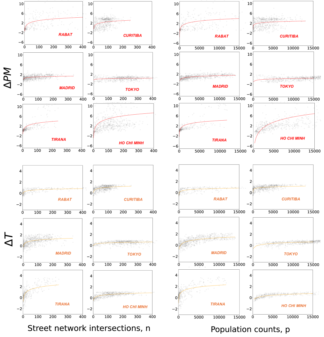
Figure 5: Logarithmic relationship between climate variables and urban characteristics. (a) Temperature results for both street network intersections and population counts. (b) Particulate matter concentration results for both street network intersections and population counts.

We start by investigating the relationship between intra-urban climate variability and urban characteristics. Our analysis shows that urban-rural differences in temperature ($\Delta T$; i.e., the magnitude of the Urban Heat Island effect) and particulate matter concentration ($\Delta PM$) are well captured by a logarithmic relationship (Equation 1 bellow) with either population count or the number of street intersections (Figure 1d and SI Figure 5 for some city examples). Explicitly, for a given grid cell $i$ in a given city, the environment-urban relationship is expressed as:

$$\Delta x_{i}=\alpha+\beta\thinspace\ln y_{i},$$ (1)

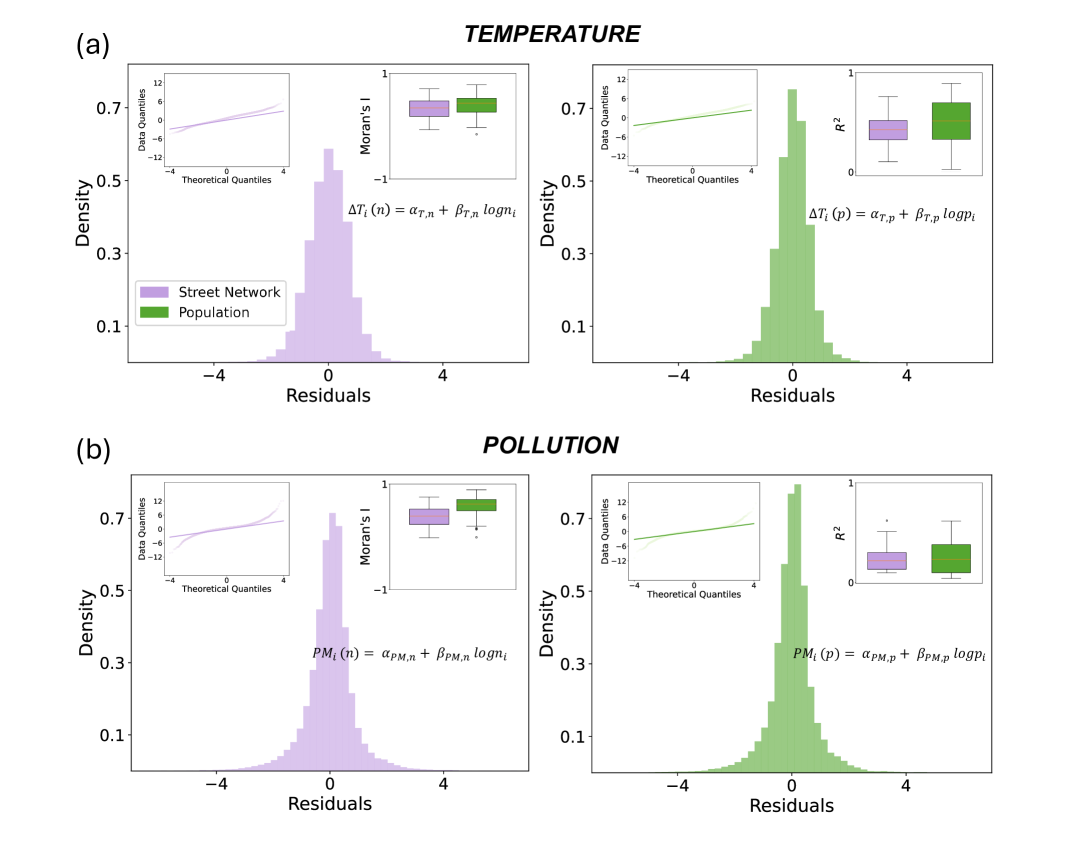
Figure 6: Aggregated city residuals and Q-Q plots for the logarithmic fits of climate varibales as a function of urban features. (a) Temperature (T), with inset showing $R^{2}$ values, Q-Q plots, and Moran’s I using a $k$-nearest neighbors (KNN) approach with $k=24$, and (b) particulate matter concentrations (PM), with inset showing $R^{2}$ values, Q-Q plots, and Moran’s I using $k=24$.

where $\alpha$ and $\beta$ are the intercept and slope, and $\Delta x_{i}$ represents the urban-rural difference for the urban grid cell $i$, relative to the average of non-urban grid cells. Such a logarithmic relationship is consistent with observed city-scale patterns [21]. Moreover, it is statistically appropriate for intra-urban fluctuations given that $T$ and $PM$ are approximately normally distributed (see SI Figure 25), while urban characteristics follow approximately log-normal distributions [45]. The residuals provided this logarithmic approach are roughly symmetrically distributed around zero with no strong heteroscedasticity, providing additional support for the adequacy of the logarithmic specification. We do observe moderate positive spatial autocorrelation (see SI Figure 6). However, this is deemed acceptable as our primary goal is not to predict fine-scale climate values in each square cell, but rather to predict aggregate statistical properties of climate variables and urban characteristics across cities. The analysis of $\alpha$ and $\beta$ across all cities reveals that their values are more consistent when derived from street intersections compared to population counts, as shown in Figure 1e where violin plots display the central 95% of the parameters estimates. This indicates that urban structure - as encoded in the transport network - is a more reliable and consistent driver of intra-urban climate variability across cities.

Applying the expected value and variance to both sides of Equation 1 yields the following expressions for the mean and standard deviation of climate variables as functions of the statistical properties of urban characteristics:

$$\langle\Delta x(y)\rangle=\alpha+\beta\langle\ln y\rangle\quad\text{,}\quad\sigma_{\Delta x}(y)=\beta\sigma_{\ln y}.$$ (2)

In the following sections, we use these expressions to characterize the probability distribution of $\Delta x$ from the statistical moments of $y$, providing a key link between quantifiable urban structure and unknown urban climate variables.

Universal scaling functions of urban climate variables

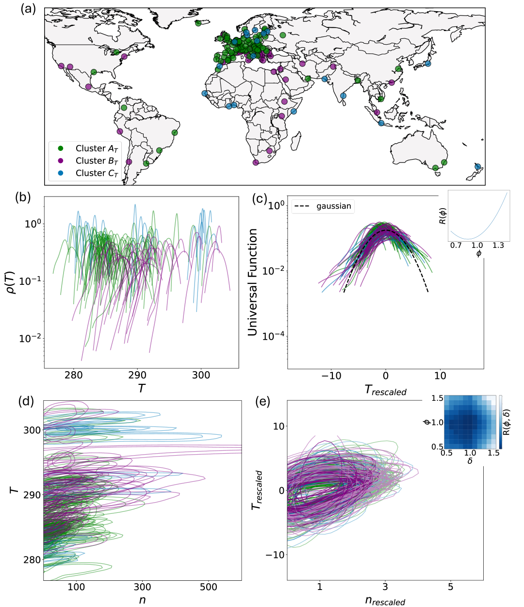
Figure 2: Universality of the intra-urban temperature ($T$) variations and covariations with street network intersections ($n$). (a) Global distribution of cities and their grouping into three clusters based on temperature data. (b) Our analysis reveals distinct probability density functions (PDFs) for the distribution of temperature in each city. (c) After rescaling according to Equations 7-4, where $T_{\text{rescaled}}=\frac{(T-T_{0})-\langle\Delta T(n)\rangle}{\sigma_{\Delta T}(n)^{\phi}}$, these PDFs collapse onto a common scaling function defined as $\sigma_{\Delta T}(n)\rho(T)$. A Gaussian fit (dashed black line) indicates that the scaling function is well approximated by a normal distribution. The inset shows the residual $R(\phi)$. (d) Our analysis also reveals distinct joint PDFs for temperature and street network intersections. (e) After both variables are properly rescaled, following Equation 5, where $n_{\text{rescaled}}=\frac{n}{\langle n\rangle^{\delta}}$, the data collapse follows a common scaling function defined as $\sigma_{\Delta T}(n)\thinspace n\thinspace\rho(T,n)$. The inset shows the residual $R(\phi,\delta)$.

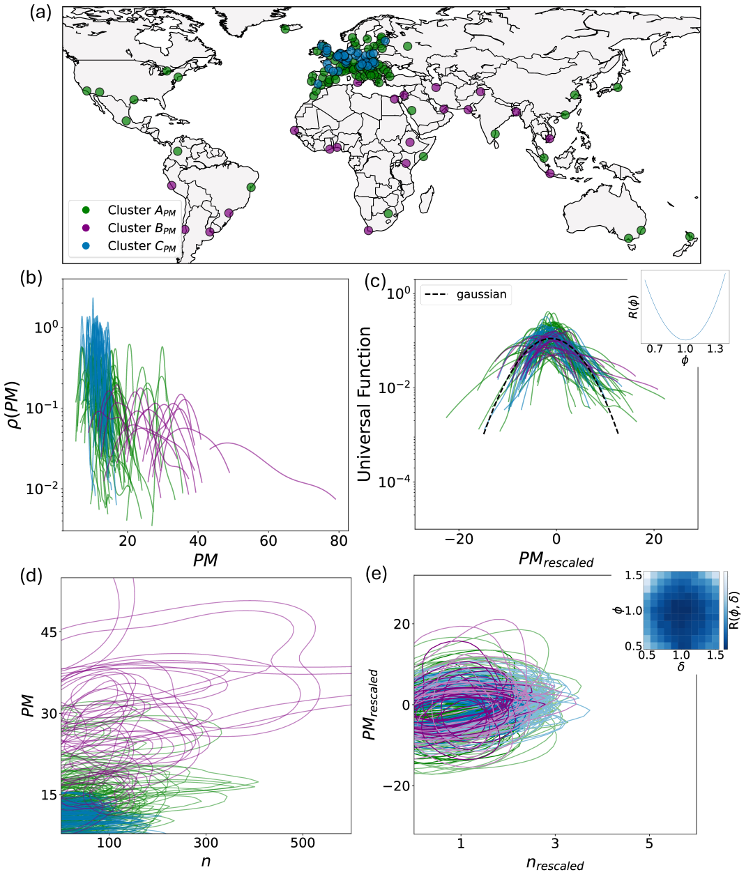
Figure 3: Universality of intra-urban air quality variations and covariations with street network intersections. (a) Global distribution of cities and their grouping into three clusters based on particulate matter concentrations ($PM$) data. (b) Our analysis reveals distinct probability density functions (PDFs) for particulate matter concentrations across cities. (b) After rescaling according to Equations 7—-4, where $PM_{\text{rescaled}}=\frac{(PM-{PM}_{0})-\langle\Delta PM(n)\rangle}{\sigma_{\Delta PM}(n)^{\phi}}$, these PDFs collapse onto a common scaling function defined as $\sigma_{\Delta PM}(n)\rho(PM)$. A Gaussian fit (dashed black line) indicates that the scaling function is well approximated by a normal distribution. The inset shows the residual $R(\phi)$. (d) Our analysis also reveals distinct joint PDFs for $PM$ and street network intersections ($n$). (e) After both variables are properly rescaled following Equation 5, where $n_{\text{rescaled}}=\frac{n}{\langle n\rangle^{\delta}}$, the data collapse follows a common scaling function defined as $\sigma_{\Delta PM}(n)\thinspace n\thinspace\rho(PM,n)$. The inset shows the residual $R(\phi,\delta)$.

The climatic conditions observed in the 142 cities show a wide range of temperature and PM values, with each city characterized by its own distinct probability density function (PDF) (Figure 2b and Figure 3b). Remarkably, after rescaling these PDFs using the statistical properties of street network intersections, we found that they all collapse onto a set of universal curves (Figure 2c and Figure 3c), thus suggesting a common underlying mechanism shaping intra-urban climate variability. Specifically, we found that the PDFs of the climate variables follow a scaling function of the form:

$$\rho(x|\langle\Delta x\rangle,\sigma_{\Delta x})=\frac{1}{\sigma_{\Delta x}^{\gamma}}F\Big{(}\frac{(x-x_{0})-\langle\Delta x\rangle}{\sigma_{\Delta x}^{\phi}}\Big{)},$$ (3)

where $F$ is a universal function across all cities, $\phi$ and $\gamma$ are the universal exponents, and $x_{0}$ refers to temperature ($T_{0}$) or particulate matter concentration ($PM_{0}$) in the rural area. The terms $\langle\Delta x\rangle$ and $\sigma_{\Delta x}$ correspond to the mean and standard deviation of climate urban-rural differences, but rather than being computed directly from the empirical $T$ and $PM_{2.5}$ distributions, they are derived from the statistical properties of the street network intersections using Equation 2. Within this framework, the rescaled climate variable is defined as:

$$x_{rescaled}=\frac{(x-x_{0})-\langle\Delta x(y)\rangle}{\sigma_{\Delta x}(y)^{\phi}},$$ (4)

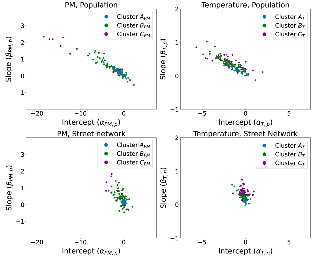
Figure 8: Slope $\beta$ vs intercept $\alpha$ plane from the logarithmic relationship between urban climate variables and urban features.

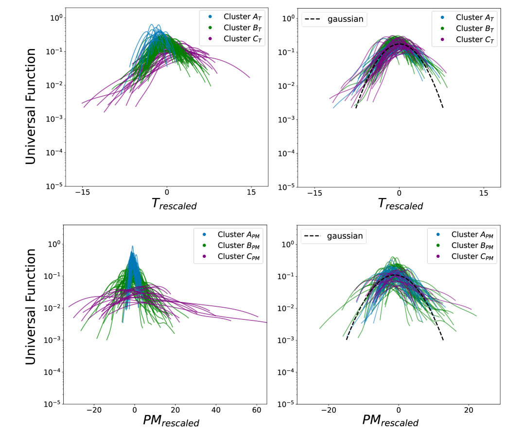
Figure 9: The data collapse results using and not using the clustering method.

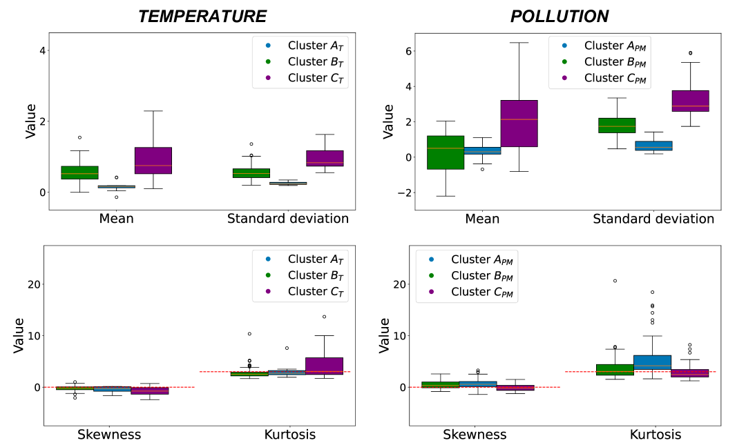
Figure 10: Mean, standard deviation, skewness, and kurtosis information of the pollution and temperature distributions per each of their three clustering groups.

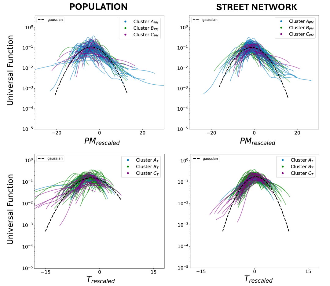
Figure 12: The data collapse results of probability density functions using population and street network intersections for $x_{rescaled}$.

where $y$ denotes the chosen urban feature (street intersections or population counts), which is used to predict $\langle\Delta x(y)\rangle$ and $\sigma_{\Delta x}(y)$ from Equation 2. While both street intersections and population counts can be used for the rescaling, using population counts yields a less robust data collapse across cities (see SI Figure 12). This suggests that urban structure, as captured by street network intersections, provides a more consistent and robust scaling framework for intra-urban climate variability than demographic metrics. We initially used a single average global intercept $\overline{\alpha}$ and slope $\overline{\beta}$ values for all 142 cities to preserve the generality of the approach. However, the data collapse for both temperature and $PM$ revealed the emergence of three distinct families of curves (see SI Figure 9). To account for these systematic differences, we grouped the cities into three clusters $k$ (see Figure 2a for temperature and Figure 3a for $PM$) based on their collapse behaviour (see Materials and Methods for details). Each cluster $k$ was then assigned its own average $\overline{\alpha}_{k}$ and slope $\overline{\beta}_{k}$. This clustering improved the overall collapse, reflecting that cities within each cluster share a more similar scaling behaviour. Even though the ($\alpha,\beta$) space does not perfectly separate the clusters, some patterns still emerge. Notably, Cluster C (Purple) tends to have higher slope ($\beta$) values, suggesting that temperature and pollution levels in these cities are more sensitive to urban features (see SI Figure 8). However, the overlap between clusters in ($\alpha,\beta$) suggests that the scaling behaviour alone does not fully explain the clustering. While the logarithmic relationship holds across all cities, the standard deviation and kurtosis of temperature and $PM$ distributions differ significantly between clusters (see SI Figure 10), whereas the standard deviation of the log of the street network intersections remains similar across them (see SI Figure 11). This suggests that the clustering does not arise solely from urban form, but rather from broader city-level processes that influence climate and pollution dynamics.

We also observe that, for temperature (Figure 2a), Cluster $A_{T}$ (blue) and Cluster $B_{T}$ (green) dominate much of Europe, the eastern United States, and Australia—regions characterized by milder temperate or humid-subtropical climates. In contrast, Cluster $C_{T}$ (purple) is prevalent across Africa and the western Americas (including Mexico, Chile, and Peru), consistent with hotter or more arid conditions. These temperature clusters therefore mirror large-scale background climates, which are known to modulate the urban heat island effect [24]. For $PM$ (Figure 3a), the Cluster $A_{PM}$ (Blue) and Cluster $B_{PM}$ (Green) prominently cover Europe, Japan, parts of the United States, and Australia, where there are relatively stricter pollution controls. Meanwhile, the Cluster $C_{PM}$ (Purple) includes high-emission areas in Asia, the Middle East, Africa, and South America, aligning with known pollution hotspots and major industrial regions.

To quantify the quality of these collapses, we employ a residual metric $R$ [46], which measures the cumulative area enclosed between all pairs of rescaled PDF curves. A lower $R$ indicates better collapse, reflecting that the rescaled curves are closer together. Minimizing $R$ confirmed that the best collapse occurs when $\phi=\gamma\approx 1$ (insets in Figures 2c and 3c), consistent with the normalization requirement $\int_{0}^{\infty}\rho(x)\,dx=1$ and the proportionality of moments (see SI Section 1 for details).

Although the exact functional form of the collapsed curves is not explicitly determined here, they are reasonably well approximated by a normal distribution (dashed black line in Figure 2c and in Figure 3c), thus supporting the choice of the logarithmic relation in Equation 1 (as the collapse of population and street intersections is approximately log-normally distributed [45], see derivation in the SI Section 1).

Universal scaling of joint probability density functions

After showing that temperature and particulate matter concentrations individually follow universal scaling functions (Equation 7), we now investigate whether similar scaling laws apply to their joint probability distributions with urban features. Since urban climate variability is influenced by multiple factors simultaneously, it is crucial to examine the coupled fluctuations of climate variables with urban characteristics.

To do so, we test whether the joint probability density functions of the climate variable $\Delta x$ and the urban feature $y$ defined as $\rho(x,y)$, satisfy the following scaling ansatz:

$$\rho(x,y\thinspace|\langle y\rangle,\thinspace\langle\Delta x\rangle,\sigma_{\Delta x})=\frac{1}{y^{\lambda}}\thinspace\frac{1}{\sigma_{\Delta x}^{\gamma}}\thinspace J\Big{(}\frac{(x-x_{0})-\langle\Delta x\rangle}{\sigma_{\Delta x}^{\phi}},\frac{y}{\langle y\rangle^{\delta}}\Big{)},$$ (5)

where $J$ is the universal scaling function and $\phi$, $\gamma$, $\lambda$, and $\delta$ are the scaling exponents. The rescaled climate variable $x_{rescaled}$ is defined as before (Equation 4), and the rescaled urban feature is defined as $y_{rescaled}=\frac{y}{\langle y\rangle^{\delta}}$, where $y$ denotes the chosen urban feature (e.g., street intersections or population counts). Figure 2e and  3e show that when $x_{\mathrm{rescaled}}$ is computed using the statistical properties of street network intersections, both $\rho(T,n)$ and $\rho(PM,n)$ achieve a robust collapse onto a single curve. To assess the quality of the data collapse, we again employ the residual metric $R$ [46], minimizing $R$ over the scaling exponents $\phi$ and $\delta$ within the same city clusters identified earlier (Figures 2a and 3a). Inset plots confirm that the best collapse occurs at $\phi\simeq\delta\simeq 1$, consistent with the normalization and proportionality of moments requirements for the climate variable (see SI for details) and for the urban feature (see [40] for details).

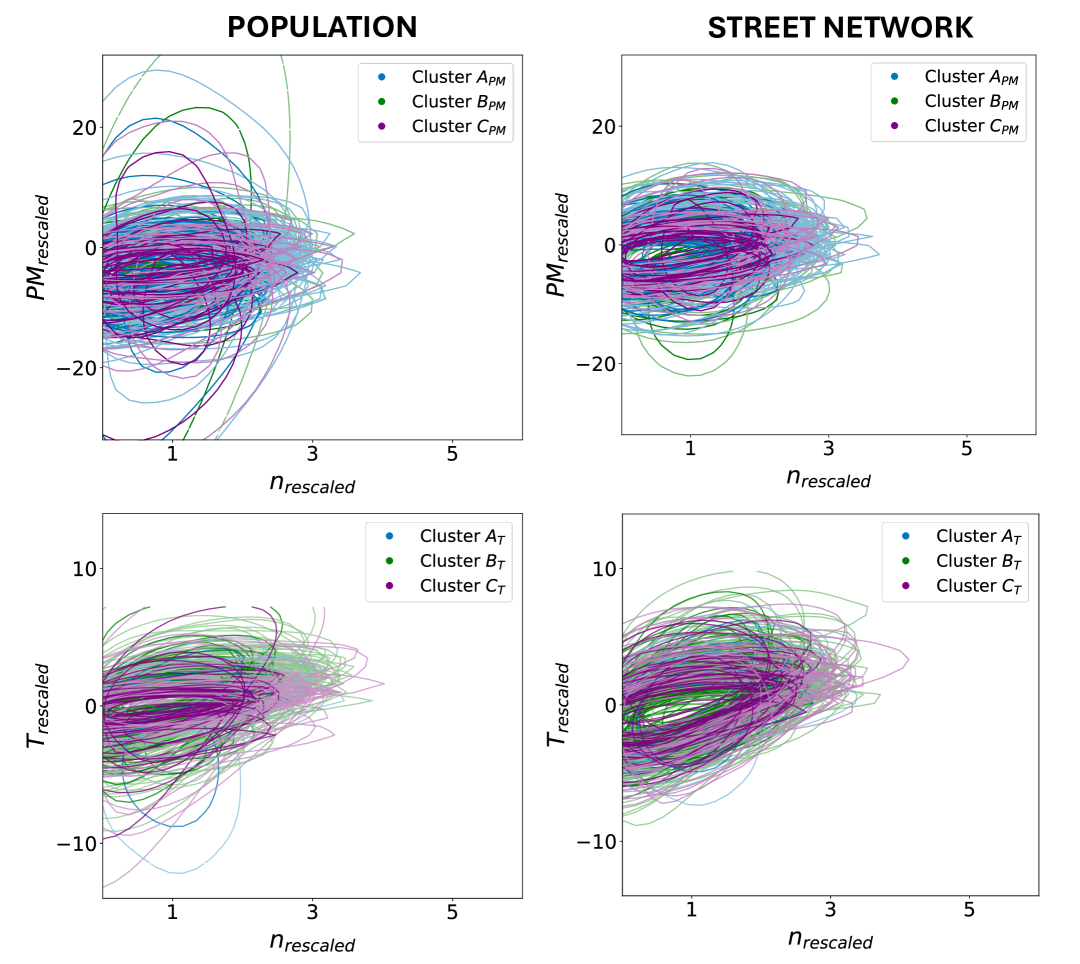
Figure 13: Data collapse results for the joint probability density functions $\rho(T,n)$ and $\rho(PM,n)$, where climate variables are rescaled ($x_{rescaled}$) using both street network intersections and population counts. The results confirm that using street network intersections for rescaling yields a more consistent collapse.

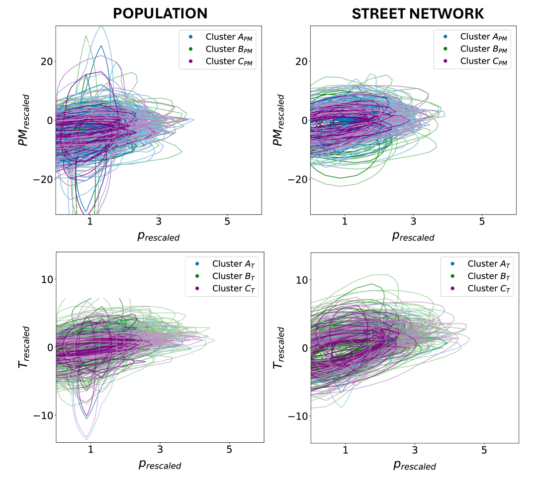
Figure 14: Data collapse results for the joint probability density functions $\rho(T,p)$ and $\rho(PM,p)$, where climate variables are rescaled ($x_{rescaled}$) using both street network intersections and population counts. Similarly, rescaling with street network intersections provides a more robust collapse compared to population counts.

As with the marginal distributions, we find that computing $x_{\mathrm{rescaled}}$ from street‐network intersections rather than population counts provides a more robust collapse (SI Figure 13 and SI Figure  14). While both $\rho(x,n)$ and $\rho(x,p)$ follow universal scaling functions, these results reinforce that urban structure is a more consistent predictor of intra‐urban climate variability than demographic metrics. Thus, when using the same street‐network–derived $x_{\mathrm{rescaled}}$, the joint probability density functions of the climate variables and population counts, $\rho(T,p)$ and $\rho(PM,p)$, similarly collapse onto a single curve (SI Figure 14).

Reconciling spatial decay models with observed probability distributions

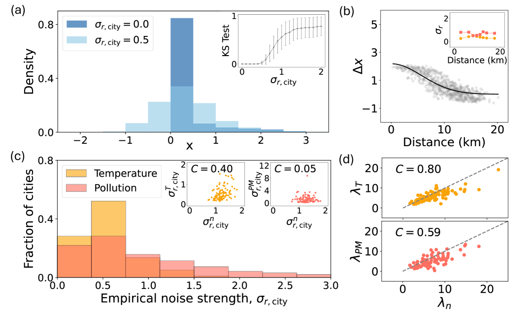
Figure 4: Linking the stochastic decay model to scaling functions of climate variables and urban street networks. (a) Probability density function resulting from the deterministic decay model ($\sigma_{r,city}=0.0$) and the numerical simulations by the proposed stochastic decay model. When using $\sigma_{r,city}=0.5$ we recover an approximately gaussian PDF shape, using a peak value $x_{A}=2.5$, decay parameter $\lambda=5$ km, and city radius $R=25$ km. The inset shows the transition from non Gaussian to Gaussian PDF shapes as we increase the white noise strength ($\sigma_{r,city}$) averaged over 1000 runs each value using the Kolmogorov-Smirnov (KS) test. (b) Temperature and particulate matter concentrations as a function of radial distance, along with the deterministic decay model fit for Bucharest. Inset shows the corresponding residual standard deviation of climate variables ($\sigma_{r}$) — computed within concentric belts. (c) Distribution of empirical noise strengths ($\sigma_{r,city}$) of climate variables across all cities. Inset shows scatter plots of the empirical noise strength of street network intersections $\sigma_{r,\text{city}}^{n}$ versus the empirical noise strength of temperature $\sigma_{r,city}^{T}$ and pollution $\sigma_{r,city}^{PM}$, along with their corresponding Pearson correlation values $C$. (d) Scatter plots of the street network decay parameter ($\lambda_{n}$) versus the decay parameters of temperature ($\lambda_{T}$) and particulate matter ($\lambda_{PM}$), along with their corresponding Pearson correlation values $C$.

Our universal scaling framework for climate variables reveals that, when appropriately rescaled by urban structure, the resulting probability distributions collapse onto a universal approximately Gaussian form (see Figure 2c, Figure 3c and SI Figure 25). However, while this probabilistic description effectively captures the statistical variability of temperature and pollution within cities, it does not provide spatial information about where these values occur. Traditional decay models — which relate urban-induced microclimate changes to the distance from the city centre [38, 47, 39] — could offer a simple spatial description that partly overcomes this problem but they yield PDFs that deviate from the observed Gaussian behaviour, following instead a $\rho(x)\propto 1/x$ form (see Figure 4a and SI Section 3 for the mathematical derivations). Here we show that this discrepancy arises from the deterministic formulation, which overlooks the significant fluctuations around the average decay trend observed in empirical data (see Figure 4b). Thus, we include an additive stochastic term in the deterministic decay function, i.e.

$$x(r)=x_{A}\exp\Bigl{(}-\tfrac{r^{2}}{2\,\lambda^{2}}\Bigr{)}+N\big{(}0,\sigma_{r,\text{city}}^{2}\big{)},$$ (6)

where $x_{A}$ is the central value at $r=0$, $\lambda$ controls the decay rate, and $N\big{(}0,\sigma_{r,\text{city}}^{2}\big{)}$ represents white noise with standard deviation $\sigma_{r,\text{city}}$, which prompts the PDFs to shift from non-Gaussian to Gaussian shapes (see Figure 4a). To quantify the strength of the stochastic component ($\sigma_{r,\text{city}}$) in the data, we compute it as the standard deviation of all residuals obtained from the deterministic decay model applied to each city’s temperature and particulate matter concentrations. Figure 4c shows the resulting distribution of city-level $\sigma_{r,\text{city}}$ values across all cities. The measured noise strength $\sigma_{r,\text{city}}$ falls within the regime necessary to recover the approximately Gaussian-shaped PDFs observed in the numerical simulations.

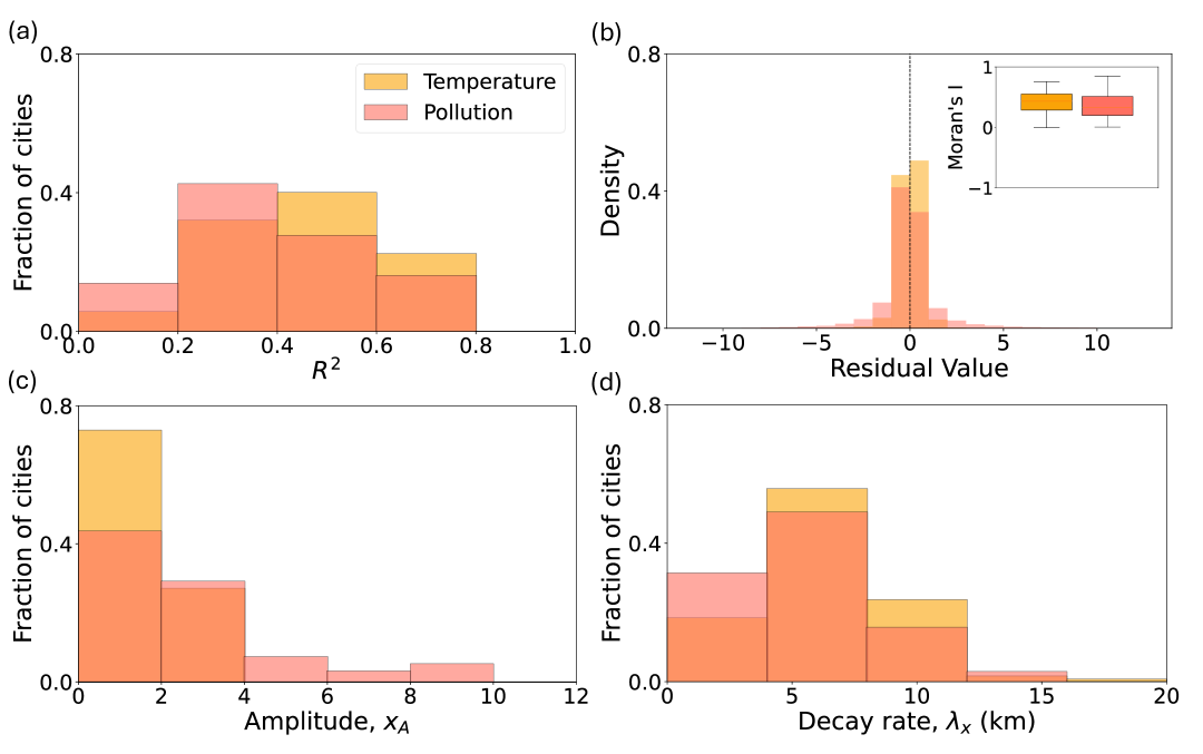
Figure 20: Decay model performance for climate variables. (a) Shows the $R^{2}$ values across all cities for both temperature and particulate matter concentrations and, (b) the histogram of all aggregated city residuals with Moran’s I (inset) using a $k$-nearest neighbors (KNN) approach with $k=24$, effectively including the first two rings of neighbors in a 1 km grid. (c) The estimated maximum amplitude at $r=0$ and (d) decay rate parameters across all cities.

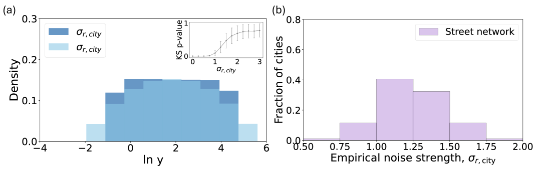
Figure 21: Linking the stochastic decay model to scaling functions of urban street networks. (a) Probability density function resulting from the deterministic decay model ($\sigma_{r}^{city}=0.0$) and the numerical simulations by the proposed stochastic decay model. When using $\sigma_{r}^{city}=1.0$ we recover an approximately gaussian PDF shape of $lny$, using a peak value $y_{A}=100$, decay parameter $\lambda_{y}=7.5km$, and city radius $R=25km$. The inset shows the transition from non gaussian to gaussian PDF shapes as we increase the white noise strength ($\sigma_{r}^{city}$) averaged over 1000 runs each value using the Kolmogorov-Smirnov (KS) test. (b) Distribution of empirical noise strengths ($\sigma_{r}^{city}$) of street network intersections across all cities.

We further explored whether the decay of urban climate variable is linked to urban structure. To do so, we also applied the exponential decay model (Equation 6) to street intersections, this time incorporating multiplicative white noise, reproducing the observed log-normal PDFs of street intersections [45] (SI Section 3, SI Figure 21). Notably, cities with stronger street intersections decay rate $\lambda_{n}$, also tend to exhibit stronger climate‐variable decay rate for temperature $\lambda_{T}$ and for $PM$ concentrations $\lambda_{PM}$ (Figure 4d). However, the correlations between the stochastic multiplicative white noise of the street intersections $\sigma_{r,city}^{n}$ and the additive white noise of climate variables $\sigma_{r,city}^{x}$ are moderate for temperature and negligible for $PM$ (insets Figure 4c), indicating that while the magnitude of fluctuations in temperature is partly linked to intersection variability, additional processes (e.g. industrial emissions, atmospheric transport) also play a role for $PM$. Temperature decay aligns more closely with urban form than $PM$ decay, reflecting the influence of non‐structural drivers on air pollution. Overall, we find that the radial decay model performs better for temperature than for particulate matter. In many cities, industrial activities cause elevated $PM$ levels at large radial distances, resulting in lower $R^{2}$ values for the $PM$ decay fit (see SI Figure 20a).

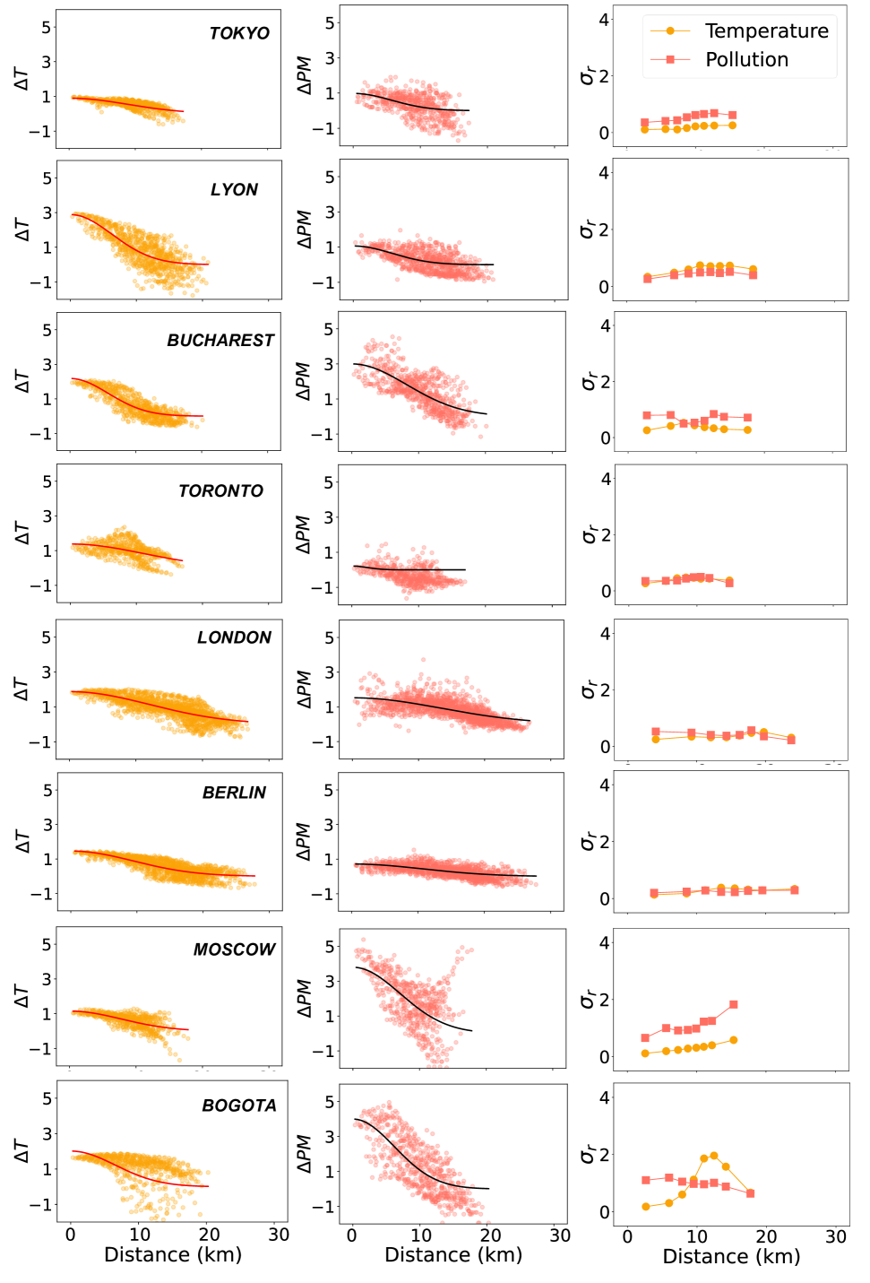
Figure 18: Temperature and particulate matter concentrations as a function of radial distance. We show the decay model results for some cities of different climate and scale along with the deterministic decay model fit and the corresponding empirical noise strength ($\sigma_{r}$) of climate variables—computed within concentric belts.

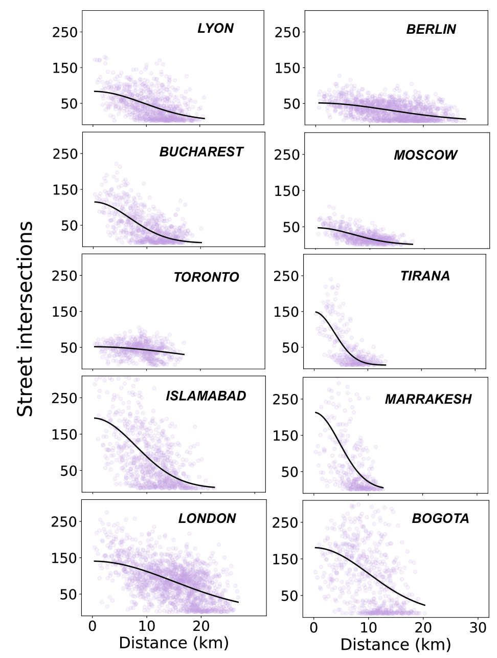
Figure 19: Street network intersections as a function of radial distance. We show the decay model results for some cities of different regions and scale along with the deterministic decay model fit.

To ensure the validity of our radial decay framework—which assumes approximate circular symmetry—we excluded cities with poor fits for the street intersection decay model ($R^{2}<0.1$), leaving 107 out of 142 cities (76%) for this spatial decay analysis. An additional 12 cities were subsequently excluded from the particulate matter ($PM$) analyses due to implausibly decay rates. We defined the city center as the mean latitude and longitude of all street intersections in the street network. Additionally, to validate the white-noise assumption for climate variables, we subdivided each city into ten concentric belts — each containing the same number of data points. For each belt, we computed the standard deviation of the residuals when using the decay-model $\sigma_{r}$. Our results show that $\sigma_{r}$ remains approximately constant across all belts for both climate variables (see inset Figure 4b). SI Figures 18 and 19 illustrate decay trends for selected cities, and SI Figures 20 and 22 provide additional details, including histograms of aggregated city residuals and model fit statistics (e.g. $R^{2}$ values).

In summary, while radial decay models capture the aggregate trend of climate variables, introducing stochasticity is essential to accurately reflect the observed fluctuations of empirical data and to recover the probability distributions and their scaling behavior predicted by the general universal scaling functions derived here. These findings provide a conceptual bridge between traditional radial-decay studies and our scaling framework, while highlighting the key role of urban structure in shaping intra-urban climate variability. In fact, this stochastic radial‐decay formulation is mathematically equivalent to assuming a city whose street network is densest at the center and progressively sparser with distance, with the added white‐noise term capturing the local fluctuations around that idealized decay link to the street network.

Discussion

We have shown that marginal and joint probability distributions of air temperature and particulate matter concentrations in cities, when rescaled by characteristic scales derived from urban features, collapse into universal scaling functions. As such, this study advances traditional scaling approaches based on city‐level metrics [24, 20, 21, 22, 23, 25, 26, 27, 28], by extending them to account for the observed intra‐urban variability of urban features.

Our stochastic approach allows to overcome problems related to the definition of city boundary [29, 30] and the neglect of local urban heterogeneities [32, 33], which would otherwise mask important microclimate effects [34, 35, 36, 37].

These results are consistent with the findings by La Porta et al. [48], who demonstrated that the probability distributions of total $CO_{2}$ and $PM$ (both emissions and concentrations) within different population ranges share a common shape (once normalized by each city’s total population). Thus, while their work reveals universal fluctuations in total $CO_{2}$ and $PM$ emissions at the city scale across different population sizes, our results extend their insight to the intra-urban level, uncovering universal behaviours driven by heterogeneous spatial structures within (and across) cities. In the context of intra-city variations, Shreevastava et al. [49, 50] investigated the patterns of remotely sensed land surface temperature in 78 cities and identified urban heat islets — i.e., clusters of high surface temperatures — characterized by fractal self-similarity and universal power-law size distributions. Thus, our results complement their findings by demonstrating that the entire variability of urban climate characteristics (defined across uniform spatial units, see Materials and Methods for details) and not just the statistics of clustered heat islets, exhibits universal scaling patterns. Here, we further demonstrate that local climate fluctuations are directly linked to urban structure, in particular to the characteristics of the street network.

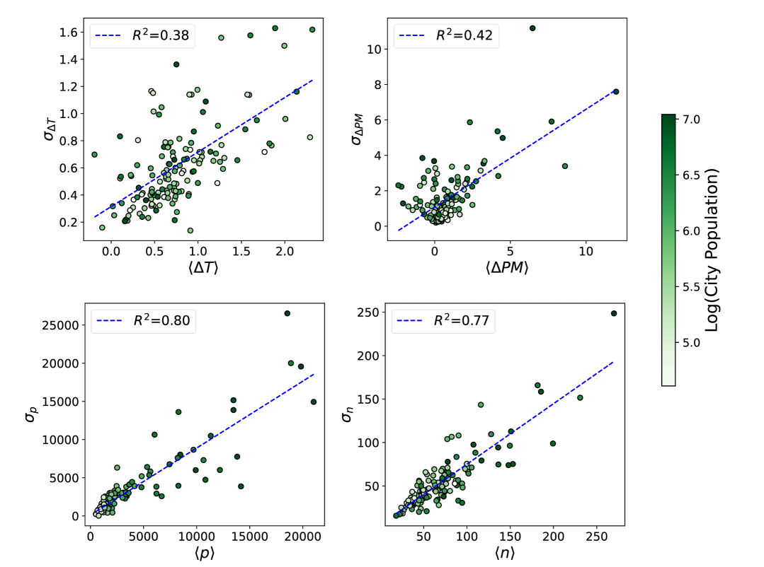
Figure 23: The mean and standard deviation of the climate and urban characteristics distributions are not fully independent across cities.

Beyond empirical validation, the specific choice of scaling function form depends primarily on the statistical properties of the distributions. For climate variables (Equation 7), the PDFs typically exhibit symmetric or nearly symmetric shapes around a mean, with mean and variance as independent parameters (see SI Figure 23). In contrast, urban features [45] often show asymmetric distributions, with the standard deviation scaling proportionally to the mean (see Figure 23). These variables are better described by log-normal distributions, which naturally account for this proportional relationship. Thus, the choice of the ansatz reflects the underlying statistical symmetry and the correlation structure between mean and variance observed in the empirical data. In fact, as shown in the SI Section 2, the Gaussian form of the rescaled climate variable $x$ can be derived from the assumption of a log-normal distribution for the urban feature $y$ combined with the logarithmic relationship between climate variable and urban feature in Equation 1. This derivation provides theoretical support for the universality of the scaling form proposed here (Equation 7).

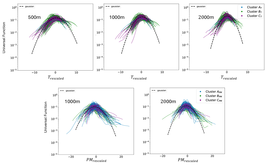
Figure 15: The results remain robust across different spatial scales of the gridding system.

Methodological robustness is confirmed through several sensitivity tests. We demonstrate scale-independence by recalculating our results using square grid cells of varying sizes (500 m, 1 km, and 2 km) while preserving spatial coherence (as four 500 m cells form one 1 km cell and four 1 km cells aggregate to form a 2 km cell, see SI Figure 15). Our findings remain consistent across these spatial scales, reinforcing the generality and reliability of the proposed scaling framework. Further robustness checks using independent datasets for both surface temperature [51] and particulate matter [52] — derived using different methodologies and varying spatial resolutions (see Material and Methods for details) — confirm that the scaling functions and resulting clustering patterns remain largely stable (see SI for details and SI Figure 16, 17). These comparisons indicate that our scaling framework is insensitive to differences in the underlying observational and modelling approaches, reinforcing the generality and reliability of the results.

It is important to note that, despite the robust scaling behaviour, we observe city groupings likely driven by factors beyond urban morphology (SI Figure 9). These groupings likely stem from external factors — such as regional climate, local emissions regulations, topography, or socioeconomic traits — that are not captured by the log‐linear dependence of urban climate on city morphology alone. Nevertheless, all the identified clusters obey the same log‐linear scaling with the chosen urban features, showing that local contexts modulate some aspects of climate variability, but the overall scaling behaviour remains valid.

A few other considerations are also worthy of note. For instance, the collapse for particulate matter is slightly less good than for temperature when rescaled by urban features — likely due to regional circulation, contributions from non-anthropogenic sources such as dust, and the localization of industrial activities in suburban areas. In addition, our current analysis focuses on static aggregated time-windows of climate variables. Further research could incorporate time dynamics to examine how the mean and standard deviation of climate variables evolve on diurnal [53, 54] and seasonal [55, 56] timescales, thereby enabling a full characterization of the corresponding climate variables probability density functions over time.

In addition, while our probabilistic description effectively captures the statistical variability of temperature and particulate matter within cities, it does not inherently provide spatial information. Traditional radial decay models [38, 47, 39] partly address this issue by offering a one-dimensional description of urban climate variation. However, they yield heavy-tailed probability density functions that deviate significantly from the Gaussian behaviour observed empirically. By incorporating an additive stochastic term into the decay model, we capture the significant fluctuations around the average decay trend, thereby recovering the observed statistical distributions. Moreover, we show that the decay trend of climate variables is strongly linked to that of street network intersections, while the strength of the additive stochastic component is only moderately associated with the multiplicative noise in street intersection for temperature. The joint probability distribution $\rho(x,y)$, between a climate variable $x$ and an urban feature $y$, confirms that higher temperatures and pollution levels statistically co‐occur with denser intersection networks. This statistical association, combined with the fact that most cities exhibit a centrally organized street network, helps explain why climate variables decay radially in space and why their spatial decay is closely tied to urban morphology. Thus, our stochastic radial-decay model — representing a “centrally organized” network with noise — successfully reproduces the observed climate distributions. This reconciliation not only underscores the necessity of accounting for stochasticity to accurately model intra-urban climate variability but also suggests that urban climate is fundamentally shaped by the interplay between the predictable decay with distance of population and infrastructure density - as explained, for example, by economic theories [e.g., 57] and gravitational models [e.g., 58] - and the randomness inherent in heterogeneous urban activities and morphologies.

In conclusion, this study provides a predictive framework based on scaling theories that fully describes intra-city fluctuations in urban microclimatic characteristics. Our results reveal that once climate variability is rescaled by appropriate urban parameters — particularly those related to street network structure — the underlying patterns become universal. This tight coupling between urban structure and the emergence of distinct climate characteristics highlights the need to radically rethink how we design and use urban spaces to minimize temperature and air pollution risks. Looking forward, our work opens new avenues for modelling urban climate across scales — from evaluating climate model outputs to downscaling regional simulations to the intra-urban level.

Future studies can evaluate model realism by testing whether the outputs of existing models, when rescaled using the statistical properties of street networks, reproduce the marginal and joint probability distributions derived here. This approach provides both an empirical benchmark and a practical framework for assessing environmental exposure and risk - as encoded in the joint probability distributions of urban features (e.g. street intersections) and climate. The simplicity of the approach makes it particularly valuable for cities with limited computational capabilities as well as for injecting climate information into reduced-complexity models of urban systems, from transport to the economy and energy sectors [59].

In general, our method offers a powerful tool for capturing both macroscopic trends across global cities and microscopic fluctuations in local microclimate, enabling extrapolation across diverse and seemingly incomparable cities. Such a framework is essential for advancing our theoretical understanding of urban complexity and its links to intra-urban climate dynamics, with significant implications for sustainable urban planning. Specifically, urban planners should consider street network morphology carefully, as areas with high street intersection density inevitably tend to experience elevated temperatures and pollution levels. Since the statistical characteristics of street networks reflect climate variability patterns, planners can proactively identify hotspots vulnerable to climate risks and implement targeted interventions — from strategic urban greening, to zoning restrictions and optimized transportation corridors.

Materials and Methods

Data Sources.

We employed mean daily ambient temperature estimates at 2 m above ground with a 100 × 100 m spatial resolution produced by the UrbClim model [60] via the VITO UrbClim FTP server (see Data and Code Availability). UrbClim was developed by the Flemish Institute for Technological Research and it integrates a land surface scheme with a three-dimensional atmospheric boundary layer module, incorporating land cover, soil sealing, vegetation, and meteorological data from the fifth-generation European Centre for Medium-Range Weather Forecasts (ECMWF) Reanalysis. For this study, temperature estimates were generated for the entire year 2017.

The annual average $PM~{2.5}$ concentrations are derived from a machine-learning-based global dataset [61]. The dataset provides daily $PM~{2.5}$ estimates at a 1 km resolution for the period 2017–2022, generated using a model that integrates multiple data sources, including satellite aerosol optical depth (AOD) retrievals (e.g., MODIS MAIAC and GEOS-FP), ground-based air quality monitoring stations ( 9500 globally), meteorological variables (e.g., temperature, humidity, wind speed), emissions inventories, and land use information. A spatiotemporally enhanced machine learning model (4D-STET) is used to fill gaps in AOD observations and to account for complex relationships between pollution, meteorology, and surface features. For this study, we use the annual average for 2022 to characterize particulate matter exposure across cities.

The street networks are extracted from OpenStreetMap (OSM) [62], an open-access, collaborative mapping project that provides continuously updated, editable maps of the world. The data is processed using OSMnx [63] to analyse the structural variability of urban transport networks, offering detailed information on streets, intersections, buildings, and other infrastructure. In this study, we specifically use this dataset to analyse street network intersections.

Finally, we use global population count data from the WorldPop dataset [64], which integrates remote sensing, census data, and geospatial technologies to produce high-resolution population distribution maps. These datasets provide consistent and comparable population estimates across urban and rural areas, with resolutions as fine as 100 meters x 100 meters in some regions. For this study, we use the unconstrained global mosaic population dataset at 1 km resolution for the year 2020, which was created using a top-down disaggregation approach based on statistical models and satellite-derived covariates. The dataset is designed to provide consistent 1 km resolution global population estimates, making it suitable for large-scale comparative urban studies.

To validate the robustness of our findings, we compare the results with other datasets and methodological approaches (see SI Section 4). For particulate matter 2.5 concentration we use also an independent dataset covering Europe downloaded from the European Environmental Agency (EEA) for the year 2022 [52]. This dataset provides annual average $PM~{2.5}$ concentrations at a 1 km resolution, derived from a regression-interpolation methodology that integrates ground-based air quality monitoring stations with satellite observations and meteorological modelling. Unlike the machine-learning-based global dataset [61], which relies on a data-driven fusion of multiple sources, this approach primarily interpolates station-based measurements to estimate $PM~{2.5}$ levels across Europe.

Similarly, to verify the consistency of our temperature results, we compare them with an independent observational dataset of global land surface temperature (LST) [51]. Unlike our primary urban climate modelling dataset [60], which simulates near-surface air temperature, the Global Summer Land Surface Temperature (LST) Grids, 2013 dataset, developed by the Center for International Earth Science Information Network (CIESIN), Columbia University, provides direct satellite-based observations of land surface temperature (LST) at a spatial resolution of 30 arc-seconds ( 1 km). The dataset is based on MODIS Aqua Level-3 (MYD11A2) Version 5 LST 8-day composite data, obtained from NASA’s Land Processes Distributed Active Archive Center (LP DAAC). This dataset reports the highest recorded daytime land surface temperature (Tmax) and the lowest recorded nighttime temperature (Tmin) observed over the peak summer months of July–August 2013 in the Northern Hemisphere and January–February 2013 in the Southern Hemisphere, ensuring that transient heat extremes are captured. In cases where cloud cover led to missing data, additional LST observations were used to fill gaps. It is important to note that LST differs from air temperature, and some regions with persistent cloud cover may contain missing or interpolated values.

Data Integration.

To ensure consistent spatial resolution across cities, we aggregate all different data into square grid cells with a side length size $l=1000\,\mathrm{m}$ (Figure 1a), partitioning the urban area into spatially uniform units for the analysis. Within each cell, we compute the mean of all temperature and $PM~2.5$ measurements, and the sum of all street‐intersection and population counts. A sensitivity analysis with different side length sizes $l$ is provided in the SI (Figure 15). We recalculate the results taking as basis square cells of side 500 m and 2 km. The cells of the different scales have been delimited to keep spatial coherence: four 500 m cells form one of the 1 km cells used in the previous figures, and four 1 km cells aggregate to form a 2 km cell. We define a distinction between urban and rural areas using the street network at 1 km $\times$ 1 km square cells resolution, specifically we consider as urban cells where there is at least one intersection ($n\geq 1$) and rural where there is only one intersection ($n=1$) to avoid water zones. We checked this method with the classification of the urban climate simulations [60], which are based on land use and built environment characteristics and found good overlap. This distinction is used to quantify traditional metrics (i.e., the UHI and UPM effects) by comparing temperature and air pollution levels between urban and non-urban grid cells.

We adopt the spatial domain provided by our UrbClim temperature dataset [60]. While previous research suggests that city structure follows consistent radial profiles that scale with population size [65], allowing for rescaled urban domains based on population-dependent functions, we find that applying such rescaling does not alter our results. In fact, we tested multiple variants of the rescaled radial extent and observed nearly identical data collapses, as long as the same criterion was applied consistently across all cities. This outcome indicates that the UrbClim model’s domain definitions already capture the relevant urban spatial scales for intra-urban climate analysis.

Statistical Analysis. We employ Kernel density estimation (KDE) [66] to derive probability density functions (PDFs) for urban climate and urban structure variables within each square cell. PDFs are computed for population counts, street network intersections, air temperature and air particulate matter concentrations, providing insights into the spatial distribution and variability of these variables within cities. In addition, the quality of the data collapse — both for marginal and joint probability density functions — is quantitatively assessed using the residual-based metric proposed in [46], which evaluates the overall distance between rescaled curves. For clearer visual presentation in the collapse plots, we removed a small fraction of cities that deviated slightly from the overall behavior: 1 city (0.7%) for temperature and 8 cities (5.6%) for PM.

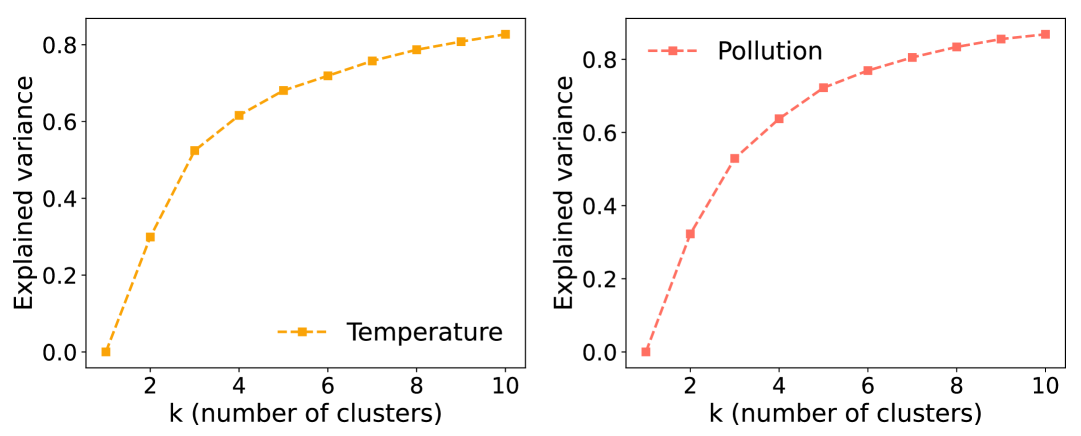
Figure 7: Temperature and pollution fraction of total variance that is explained by a K-means partition as a function of the number of clusters $k$. The curve rises steeply up to $k\approx 3$ and then flattens in both variables, indicating diminishing returns from introducing additional clusters.

Clustering. We employ the K-means clustering method [67]. For each city, we first compute the normalized climate distribution using a global intercept $\overline{\alpha}$ and slope $\overline{\beta}$ values averaged across all 142 cities (see SI Figure 9)—and summarize its form by the coordinates of its maximum density point, $(x_{peak},y_{peak})$. Thus, each city is represented by the two-component feature vector. We run K-means for $k=1,\dots,10$, which partitions cities by minimizing the within-cluster sum of squared Euclidean distances in the two-dimensional $(x_{\rm peak},y_{\rm peak})$ space. The optimal number of clusters is selected using the elbow of the within-cluster sum-of-squares, expressed as explained variance. In both temperature and pollution data the elbow occurs at $k=3$ (see SI Figure 7). Finally, to ensure the tightest possible collapse of the rescaled curves, we recomputed the Bhattacharjee et al. residual metric $R$ [46] and found that only 4.2% for temperature (6 cities) and 8.4% for pollution (12 cities) changed cluster assignment, confirming the robustness of our grouping—and very low computational cost.

Figures and Tables

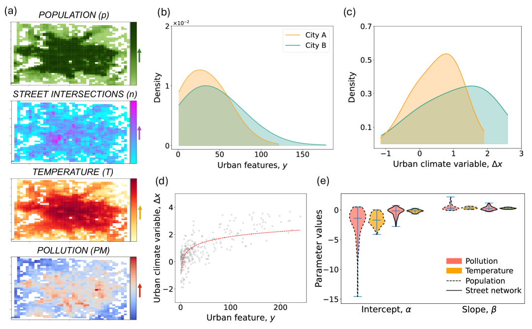
Figure 1: Relationship between intra-urban climate variables variability and urban features. (a) Illustration of temperature ($T$), particulate matter concentrations ($PM$), street network intersections ($n$) and population ($p$) obtained by discretizing the space into spatial units of square grid cells for Berlin (Germany). (b) Empirical probability density function of urban climate and (c) urban features for two example cities. (d) Logarithmic scaling relationship between intra-urban climate variability and urban features. (e) Comparative analysis of the intercept ($\alpha$) and the slope ($\beta$) of the logarithmic relationship between intra‐urban climate variability and urban features across all cities. Violin plots display the central 95% of the parameters estimates, highlighting that street network is more consistent and robust than population counts.

Author Contributions

G.M. acquired the funding, conceived, and supervised the project. M.D.S. devised and performed the analyses and drafted the manuscript with inputs from M.H. and G.M. All authors interpreted the results, provided feedback that helped shape the analysis, and contributed to writing the manuscript.

Competing Interests

The authors declare no competing interests.

Data and Code Availability

The datasets utilized in this study are publicly available from the following sources: population count data from https://hub.worldpop.org/, street network data from https://www.openstreetmap.org/, temperature data from https://provide.marvin.vito.be/ftp/compressed_daily/ and https://www.earthdata.nasa.gov, and PM2.5 data from https://zenodo.org/records/10800980 and https://www.eea.europa.eu/en.

The Jupyter notebooks and associated scripts necessary to reproduce the results of this paper are accessible on GitHub at https://github.com/marcduransala2000/intra_urban_climate_scaling.

Supplementary Information

1

Scaling exponents. This derivation follows the same approach used in scaling analyses, where normalization and moment proportionality requirements impose constraints on scaling exponents (e.g., [40], although applied to a different scaling form).

Normalization.

Here, we show that the normalization requirement $\int_{-\infty}^{\infty}\rho(x)\,dx=1$ for climate distributions of the form

$$\rho(x\,|\,\langle\Delta x\rangle,\sigma_{\Delta x})=\frac{1}{\sigma_{\Delta x}^{\gamma}}\,F\left(\frac{(x-x_{0})-\langle\Delta x\rangle}{\sigma_{\Delta x}^{\phi}}\right)$$ (7)

constraints the possible values of the scaling exponents $\gamma$ and $\phi$.

By performing the change of variables

$$u=\frac{x-x_{0}-\langle\Delta x\rangle}{\sigma_{\Delta x}^{\phi}},\quad\text{so that}\quad dx=\sigma_{\Delta x}^{\phi}\,du,$$

the normalization condition becomes:

$$\int_{-\infty}^{\infty}\rho(x\,|\,\langle\Delta x\rangle,\sigma_{\Delta x})\,dx=\sigma_{\Delta x}^{\phi-\gamma}\int_{-\infty}^{\infty}F(u)\,du=1\Rightarrow\phi=\gamma$$ (8)

Proportionality of moments. Let us look at a generic $j$-th central moment, defined for convenience about the shift $\langle\Delta x\rangle$:

$$\langle\bigl{[}(x-x_{0})-\langle\Delta x\rangle\bigr{]}^{j}\rangle=\int_{-\infty}^{\infty}\bigl{[}(x-x_{0})-\langle\Delta x\rangle\bigr{]}^{j}\,\rho(x)\,dx.$$ (9)

Using the same change of variable $u$ as before, one gets:

$$\langle\bigl{[}(x-x_{0})-\langle\Delta x\rangle\bigr{]}^{j}\rangle =\int_{-\infty}^{\infty}\bigl{(}\sigma_{\Delta x}^{\phi}\,u\bigr{)}^{j}\frac{1}{\sigma_{\Delta x}^{\gamma}}F(u)\,\sigma_{\Delta x}^{\phi}\,du$$

$$=\sigma_{\Delta x}^{\phi j+\phi-\gamma}\int_{-\infty}^{\infty}u^{j}\,F(u)\,du,$$ (10)

therefore, as we previously showed that $\gamma=\phi$, we can write:

$$\langle\bigl{[}(x-x_{0})-\langle\Delta x\rangle\bigr{]}^{j}\rangle=\sigma_{\Delta x}^{\phi j}\,\int_{-\infty}^{\infty}u^{j}\,F(u)\,du.$$ (11)

More explicitly:

• For $j=1$, we get the first central moment $\langle(x-x_{0}-\langle\Delta x\rangle)\rangle=\sigma_{\Delta x}^{\phi}\int u\,F(u)\,du.$ By requiring $\int u\,F(u)\,du=0$, we ensure that $\langle\Delta x\rangle$ is the mean shift.

• For $j=2$, we get $\langle(x-x_{0}-\langle\Delta x\rangle)^{2}\rangle=\sigma_{\Delta x}^{2\phi}\int u^{2}\,F(u)\,du.$ By requiring $\int u^{2}\,F(u)\,du=1$ and $\phi=1$, we identify $\sigma_{\Delta x}$ as the standard deviation.

2

Urban climate universal scaling form. Previous studies [45, 44] have shown that urban variables $y$ (such as population, street intersections, etc.) can be described through their probability density function $p(y)$ according to the scaling form:

$$p(y\mid\langle y\rangle)=y^{-\lambda}\,F\left(\frac{y}{\langle y\rangle^{\delta}}\right),$$ (12)

with scaling exponents $\lambda,\delta$ and mean $\langle y\rangle$.

For simplicity, we can reasonably assume that the urban feature $y$ follows a lognormal distribution (REF):

$$\log y\sim\mathcal{N}\!\bigl{(}\langle\log y\rangle,\;\sigma_{\log y}^{2}\bigr{)}\;\;\Longrightarrow\;\;p(y)=\frac{1}{y\sqrt{2\pi\sigma_{\log y}^{2}}}\,\exp\!\!\left[-\frac{(\log y-\langle\log y\rangle)^{2}}{2\sigma_{\log y}^{2}}\right].$$ (13)

In this paper use use a log–linear relationship to link climate variable and the urban feature:

$$\Delta x=\alpha+\beta\log y\;\quad\Longleftrightarrow\quad y=\exp\!\Bigl{[}\tfrac{\Delta x-\alpha}{\beta}\Bigr{]},$$ (14)

where $\alpha$ and $\beta$ take cluster‑specific averages $(\bar{\alpha}_{k},\bar{\beta}_{k})$. From (14) we get:

$$\left|\frac{dy}{d\Delta x}\right|=\frac{1}{\beta}\exp\!\Bigl{[}\tfrac{\Delta x-\alpha}{\beta}\Bigr{]}=\frac{y}{\beta}.$$

The PDF of $\Delta x$ is therefore:

$$p_{\Delta x}(\Delta x) =p_{y}(y)\;\left|\frac{dy}{d\Delta x}\right|$$

$$=\frac{1}{\beta\sqrt{2\pi\sigma_{\log y}^{2}}}\,\exp\!\Bigl{[}-\tfrac{(\log y-\langle\log y\rangle)^{2}}{2\sigma_{\log y}^{2}}\Bigr{]}\Bigg{|}_{\,\log y=\frac{\Delta x-\alpha}{\beta}}$$

$$=\frac{1}{\beta\sqrt{2\pi\sigma_{\log y}^{2}}}\,\exp\!\Bigl{[}-\tfrac{\bigl{(}\frac{\Delta x-\alpha}{\beta}-\langle\log y\rangle\bigr{)}^{2}}{2\sigma_{\log y}^{2}}\Bigr{]}.$$ (15)

Using the mean $\langle\Delta x\rangle=\alpha+\beta\mu$ and variance $\sigma_{\Delta x}=\beta\sigma_{\log y}$, (15) simplifies to:

$$p_{\Delta x}(\Delta x)=\frac{1}{\sigma_{\Delta x}\sqrt{2\pi}}\,\exp\!\Bigl{[}-\tfrac{(\Delta x-\langle\Delta x\rangle)^{2}}{2\sigma_{\Delta x}^{2}}\Bigr{]}.$$ (16)

Thus, we shown that $\Delta x$ is normally distributed.

By defining the location and scale parameters as:

$$\mu:=\langle\Delta x\rangle=\alpha+\beta\langle\log y\rangle\quad\text{and}\quad S:=\sigma_{\Delta x}=\beta\,\sigma_{\log y},$$ (17)

that are both computed from the urban feature, we can rewrite (16) as:

$$p_{\Delta x}(\Delta x)=S^{-1}\;F\!\Bigl{(}\tfrac{\Delta x-\mu}{S}\Bigr{)},$$ (18)

where the universal function

$$F(u)=\frac{1}{\sqrt{2\pi}}e^{-u^{2}/2},$$

is the same for every city once the data are rescaled by $S$.

Equation (18) corresponds exactly to the scaling form given in Equation (7) we used in the main text and that constitutes our key expression to emphasize the universality across cities. We deliberately avoid explicitly referring to the Gaussian distribution in the main text, and instead present a more general formulation through the function $F$. This choice reflects that a perfect Gaussian shape would only be expected in the infinite-size limit, according to the central limit theorem, and under the assumption that the random variables are strictly independent and identically distributed (i.i.d.).

3

Radial decay model of climate variables. The model developed by [38, 47, 39], assuming a circular city of radius R and a radially decaying climate variable, is given by:

$$x(r)\;=\;x_{A}\,\exp\!\Bigl{(}-\tfrac{r^{2}}{2\,\lambda^{2}}\Bigr{)},$$ (19)

where $x_{A}$ is the central value at $r=0$, and $\lambda$ controls the decay rate of the climate variable.

To derive the distribution of values $x$, we note that a ring at radius $r$ has area $\mathrm{d}A=2\pi r\,\mathrm{d}r$. Since $x$ decreases with $r$, the probability density $\rho(x)\,\mathrm{d}x$ is proportional to the fraction of area between $r$ and $r+\mathrm{d}r$, yielding:

$$\rho(x)\,\mathrm{d}x\;=\;\frac{dA}{A}\;=\;\frac{2\,r}{R^{2}}\,\bigl{|}\tfrac{\mathrm{d}r}{\mathrm{d}x}\bigr{|}\,\mathrm{d}x\quad\Longrightarrow\quad\rho(x)=\frac{2\,r}{R^{2}}\,\bigl{|}\tfrac{\mathrm{d}r}{\mathrm{d}x}\bigr{|}.$$ (20)

From Equation (19), we can write $\ln(x/x_{A})=-\tfrac{r^{2}}{2\lambda^{2}}$, that gives

$$r=\lambda\,\sqrt{-\,2\,\ln\!\Bigl{(}\tfrac{x}{x_{A}}\Bigr{)}}\quad\text{and}\quad\frac{\mathrm{d}r}{\mathrm{d}x}=-\frac{\lambda^{2}}{r\,x}.$$ (21)

All together, we obtain:

$$\rho(x)=\frac{2\,\lambda^{2}}{R^{2}}\,\frac{1}{x},$$ (22)

that is valid for $x\in\big{[}\,x_{A}\,e^{-\,R^{2}/(2\,\lambda^{2})},\,x_{A}\big{]}$. One can verify that $\int\rho(x)\,\mathrm{d}x=1$, so we obtain $\rho(x)\propto 1/x$.

Adding additive white noise. Empirical data exhibit fluctuations around the deterministic decay in Equation (19). To capture these fluctuations, we add an additive noise term:

$$x(r)\;=\;x_{A}\exp\Bigl{(}-\tfrac{r^{2}}{2\,\lambda^{2}}\Bigr{)}\;+\;\mathcal{N}(0,\,\sigma_{r,\text{city}}^{2}).$$ (23)

Here, the noise strength $\sigma_{r,\text{city}}$ has the same units as $x$. This white noise convolves the original deterministic distribution $\rho(x)\propto 1/x$ with a Gaussian kernel. When $\sigma_{r,\text{city}}$ is small, the $1/x$ shape is only slightly blurred; for large noise, the distribution may significantly deviate from $1/x$, approaching a Gaussian — matching what is observed in empirical climate data.

Radial decay model of urban features. For an urban metric $y$ (e.g., intersection density, building density) we use the same deterministic form:

$$y(r)\;=\;y_{A}\,\exp\!\Bigl{(}-\tfrac{r^{2}}{2\,\lambda_{y}^{2}}\Bigr{)},$$ (24)

where $y_{A}$ is the central value at $r=0$, and $\lambda_{y}$ controls the decay rate of the urban feature. Repeating the above derivations gives $\rho(y)\propto 1/y$.

Adding multiplicative white noise. To better reproduce the empirical distribution of urban features, we follow the same approach used for climate variables, but now fluctuations are multiplicative rather than additive. Thus, we add a multiplicative white noise to Equation 24 as:

$$y(r)=y_{A}\,\exp\!\Bigl{(}-\tfrac{r^{2}}{2\,\lambda_{y}^{2}}\Bigr{)}e^{\epsilon}\quad\text{with}\quad\epsilon\sim\mathcal{N}(0,\sigma_{r,\text{city}}^{2})$$ (25)

or, equivalently:

$$\ln y(r)\;=\;\Bigl{[}\ln y_{A}-\frac{r^{2}}{2\lambda_{y}^{2}}\Bigr{]}\;+\;\mathcal{N}\!\bigl{(}0,\sigma_{r,\text{city}}^{2}\bigr{)}$$ (26)

where the noise strength $\sigma_{r,\text{city}}$ is dimensionless. This white noise convolves the deterministic distribution $\rho(\ln y)$ with a Gaussian kernel. As the noise strength increases, the resulting distribution becomes Gaussian:

$$\rho(\ln y)\sim\text{gaussian}\quad\Longrightarrow\quad\rho(y)\sim\text{log-normal}$$ (27)

reproducing the empirical findings of log-normal PDFs for urban features [45].

4

Validation with alternative datasets. To further assess the robustness of our results, we validated the scaling functions using independent methodological datasets for both climate variables (see Methods in the main text for details).

First, we analyzed the PM results using an independent European dataset at a 1 km resolution for the same year [52]. While our primary global dataset relies on a machine-learning approach integrating satellite aerosol optical depth retrievals, ground-based monitoring stations, and meteorological data, the European dataset employs a regression-interpolation framework that spatially extrapolates PM values from monitoring networks. Despite methodological differences, the scaling functions remain valid, confirming the robustness of our scaling framework (Figure 17). Furthermore, the clustering structure remains largely consistent across datasets, reinforcing the stability of the observed patterns. Both datasets reveal two dominant PM clusters in Europe, with the higher-resolution European dataset enhancing the separation between eastern and western European cities. This indicates that the broad-scale PM patterns observed globally persist across resolutions and methodologies, highlighting the resilience of the scaling framework.

Similarly, we validated the consistency of our temperature results using an independent observational dataset of land surface temperature (LST) at 1 km resolution [51]. The datasets correspond to different years and differ methodologically: our primary dataset is based on high-resolution urban climate modeling estimating near-surface air temperature, while the comparison dataset provides satellite-derived land surface temperature (Tmax), representing the highest recorded daytime temperatures during summer months. Despite these methodological differences, the scaling functions remain valid in both cases (Figure 16). However, clustering analyses reveal differing behaviors. Specifically, summer land surface temperature (Tmax) exhibits a more compressed Gaussian distribution, resulting in limited clustering differentiation compared to the wider distribution of annual air mean temperatures, which better discriminates distinct climatic regimes. This suggests that the yearly air mean temperature captures a broader spectrum of intra-urban climate variability, enabling clearer climatic differentiation across cities.

Thus, despite methodological variations, our scaling framework remains robust for both climate variables, further demonstrating its general applicability.

Figures and Tables

Figure 11: Mean and standard deviation of the logarithm of street intersection values for each of the three temperature and pollution clustering groups.

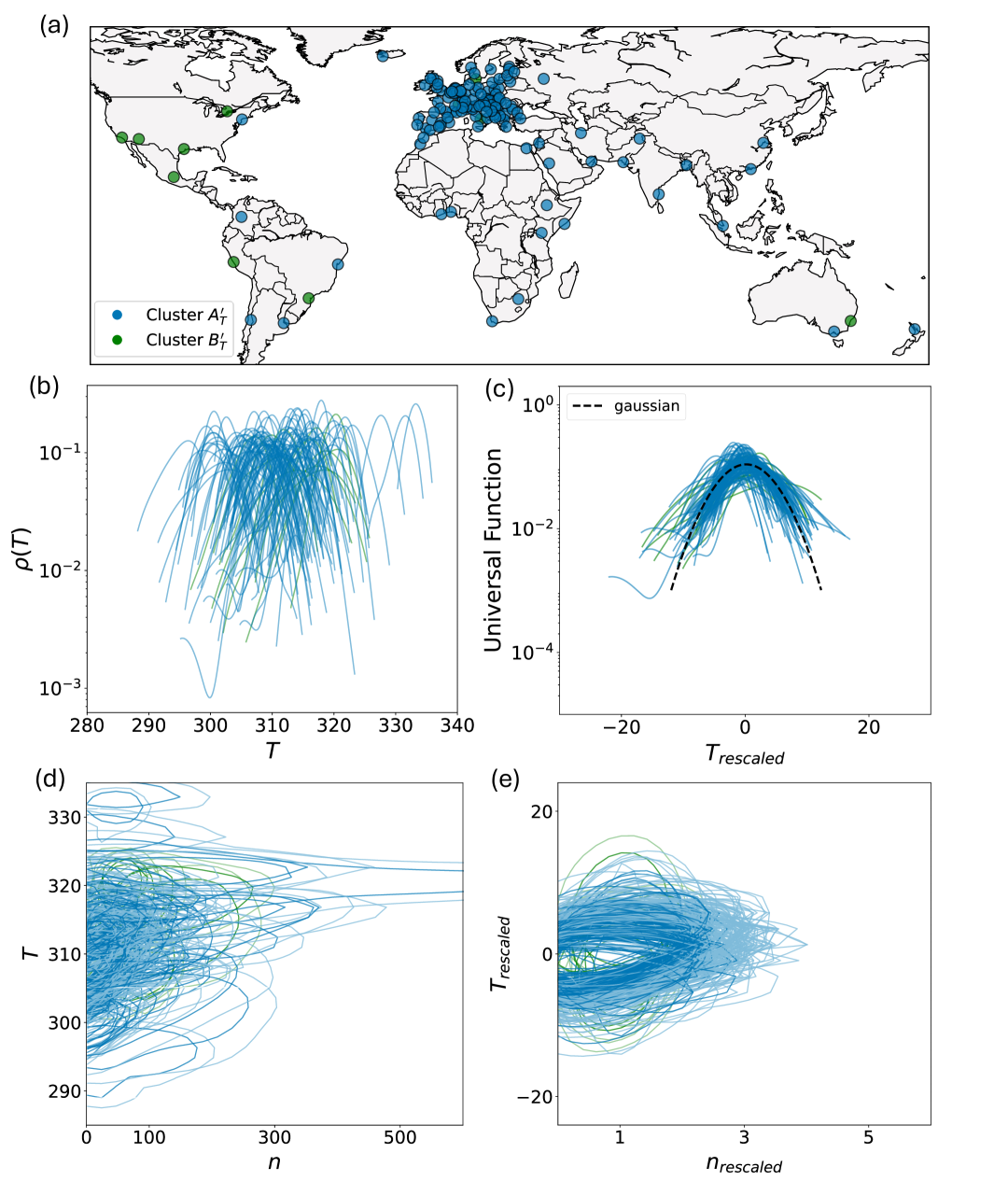
Figure 16: Confirming the robustness of the underlying scaling framework using observational maximum land surface temperature (LST) data during Summer months 2013.

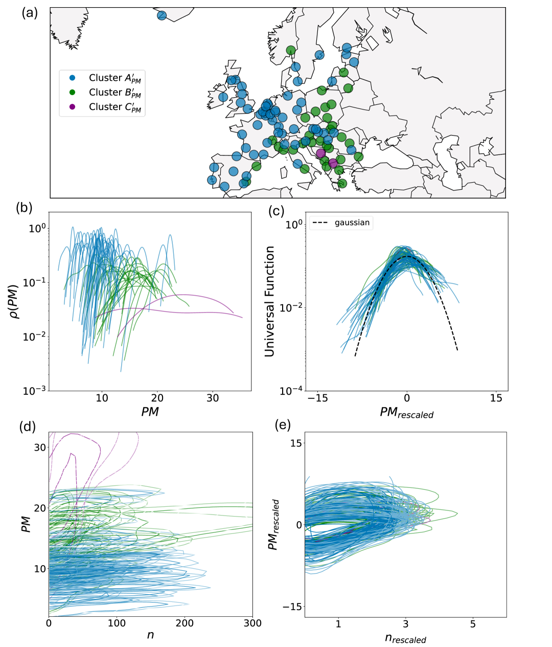
Figure 17: Confirming the robustness of the underlying scaling framework using a regression-interpolation framework from pollution ground-based monitoring stations in Europe during 2022.

Figure 22: Decay model performance for street network. (a) Shows the $R^{2}$ values across all cities for both temperature and particulate matter concentrations and, (b) the histogram of all aggregated city residuals (c) The estimated maximum amplitude at $r=0$ and (d) decay rate parameters across all cities.

Figure 24: Pearson correlation between variables and Moran’s I values used to assess spatial autocorrelation using a $k$-nearest neighbors (KNN) approach with $k=24$.

Figure 25: Climate variables are approximately gaussian shaped and urban characteristics approximately log normal shaped. Boxplots illustrating skewness and kurtosis for the four analyzed variables—log node, log population, temperature, and PM—across all sampled cities.

References

- Huang et al. [2023] Wan Ting Katty Huang, Pierre Masselot, Elie Bou-Zeid, Simone Fatichi, Athanasios Paschalis, Ting Sun, Antonio Gasparrini, and Gabriele Manoli. Economic valuation of temperature-related mortality attributed to urban heat islands in european cities. Nature Communications, 14(1):7438, Nov 2023. ISSN 2041-1723. doi: 10.1038/s41467-023-43135-z. URL https://doi.org/10.1038/s41467-023-43135-z.
- Estrada et al. [2017] Francisco Estrada, W. J. Wouter Botzen, and Richard S. J. Tol. A global economic assessment of city policies to reduce climate change impacts. Nature Climate Change, 7(6):403–406, Jun 2017. ISSN 1758-6798. doi: 10.1038/nclimate3301. URL https://doi.org/10.1038/nclimate3301.
- Khomenko et al. [2021] Sasha Khomenko, Marta Cirach, Evelise Pereira-Barboza, Natalie Mueller, Jose Barrera-Gómez, David Rojas-Rueda, Kees de Hoogh, Gerard Hoek, and Mark Nieuwenhuijsen. Premature mortality due to air pollution in european cities: a health impact assessment. The Lancet Planetary Health, 5(3):e121–e134, 2021.
- Maji et al. [2017] Kamal Jyoti Maji, Anil Kumar Dikshit, and Ashok Deshpande. Disability-adjusted life years and economic cost assessment of the health effects related to pm2.5 and pm10 pollution in mumbai and delhi, in india from 1991 to 2015. Environmental Science and Pollution Research, 24(5):4709–4730, Feb 2017. ISSN 1614-7499. doi: 10.1007/s11356-016-8164-1. URL https://doi.org/10.1007/s11356-016-8164-1.
- United Nations [2018] United Nations. 2018 revision of world urbanization prospects, 2018. URL https://population.un.org/wup/.
- Grimm et al. [2008] Nancy Grimm, Stanley Faeth, Nancy Golubiewski, Charles Redman, Jianguo Wu, Xuemei Bai, and John Briggs. Global change and the ecology of cities. Science (New York, N.Y.), 319:756–60, 03 2008. doi: 10.1126/science.1150195.
- Rydin et al. [2012] Yvonne Rydin, Ana Bleahu, Michael Davies, Julio D Dávila, Sharon Friel, Giovanni De Grandis, Nora Groce, Pedro C Hallal, Ian Hamilton, Philippa Howden-Chapman, et al. Shaping cities for health: complexity and the planning of urban environments in the 21st century. The lancet, 379(9831):2079–2108, 2012.
- Chapman et al. [2017] Sarah Chapman, James E. M. Watson, Alvaro Salazar, Marcus Thatcher, and Clive A. McAlpine. The impact of urbanization and climate change on urban temperatures: a systematic review. Landscape Ecology, 32(10):1921–1935, Oct 2017. ISSN 1572-9761. doi: 10.1007/s10980-017-0561-4. URL https://doi.org/10.1007/s10980-017-0561-4.
- Wang et al. [2019] Qiang Wang, Mei-Po Kwan, Kan Zhou, Jie Fan, Yafei Wang, and Dongsheng Zhan. The impacts of urbanization on fine particulate matter (pm2.5) concentrations: Empirical evidence from 135 countries worldwide. Environmental Pollution, 247:989–998, 2019. ISSN 0269-7491. doi: https://doi.org/10.1016/j.envpol.2019.01.086. URL https://www.sciencedirect.com/science/article/pii/S0269749118340314.
- Mills [2014] Gerald Mills. Urban climatology: History, status and prospects. Urban Climate, 10:479–489, 2014. ISSN 2212-0955. doi: https://doi.org/10.1016/j.uclim.2014.06.004. URL https://www.sciencedirect.com/science/article/pii/S2212095514000443. Measurement and modelling of the urban atmosphere in the present and the past.
- Oke et al. [2017] T. R. Oke, G. Mills, A. Christen, and J. A. Voogt. Urban Climates. Cambridge University Press, 2017. ISBN 9781139016476. doi: 10.1017/9781139016476. Online publication date: September 2017.
- Stewart [2019] Iain D. Stewart. Why should urban heat island researchers study history? Urban Climate, 30:100484, 2019. ISSN 2212-0955. doi: https://doi.org/10.1016/j.uclim.2019.100484. URL https://www.sciencedirect.com/science/article/pii/S2212095519300203.
- Lobo et al. [2023] José Lobo, Rimjhim M. Aggarwal, Marina Alberti, Melissa Allen-Dumas, Luís M. A. Bettencourt, Christopher Boone, Christa Brelsford, Vanesa Castán Broto, Hallie Eakin, Sharmistha Bagchi-Sen, Sara Meerow, Celine D’Cruz, Aromar Revi, Debra C. Roberts, Michael E. Smith, Abigail York, Tao Lin, Xuemei Bai, William Solecki, Diane Pataki, Luís Bojorquez Tapia, Marcy Rockman, Marc Wolfram, Peter Schlosser, and Nicolas Gauthier. Integration of urban science and urban climate adaptation research: opportunities to advance climate action. npj Urban Sustainability, 3(1):32, Jun 2023. ISSN 2661-8001. doi: 10.1038/s42949-023-00113-0. URL https://doi.org/10.1038/s42949-023-00113-0.
- Manoli [2025] G. Manoli. Urban climate from the lens of complexity science. In Diego Rybski, editor, Compendium of Urban Complexity. Springer Nature, 2025. ISBN 978-3-031-82665-8. In Compendium of Urban Complexity.
- Batty [2009] Michael Batty. Cities as Complex Systems: Scaling, Interaction, Networks, Dynamics and Urban Morphologies, pages 1041–1071. Springer New York, New York, NY, 2009. ISBN 978-0-387-30440-3. doi: 10.1007/978-0-387-30440-3˙69. URL https://doi.org/10.1007/978-0-387-30440-3_69.
- Bettencourt [2021] Luís M. A. Bettencourt. Introduction to Urban Science: Evidence and Theory of Cities as Complex Systems. The MIT Press, 2021. ISBN 9780262366441. doi: 10.7551/mitpress/13909.001.0001.
- Caldarelli et al. [2023] G. Caldarelli, E. Arcaute, M. Barthelemy, M. Batty, C. Gershenson, D. Helbing, S. Mancuso, Y. Moreno, J. J. Ramasco, C. Rozenblat, A. Sánchez, and J. L. Fernández-Villacañas. The role of complexity for digital twins of cities. Nature Computational Science, 3(5):374–381, May 2023. ISSN 2662-8457. doi: 10.1038/s43588-023-00431-4. URL https://doi.org/10.1038/s43588-023-00431-4.
- West and Brown [2005] Geoffrey B. West and James H. Brown. The origin of allometric scaling laws in biology from genomes to ecosystems: towards a quantitative unifying theory of biological structure and organization. Journal of Experimental Biology, 208(Pt 9):1575–1592, May 2005. doi: 10.1242/jeb.01589.
- Kleiber et al. [1932] Max Kleiber et al. Body size and metabolism. Hilgardia, 6(11):315–353, 1932.
- Oke [1973] T.R. Oke. City size and the urban heat island. Atmospheric Environment (1967), 7(8):769–779, 1973. ISSN 0004-6981. doi: https://doi.org/10.1016/0004-6981(73)90140-6. URL https://www.sciencedirect.com/science/article/pii/0004698173901406.
- Li et al. [2020] Yunfei Li, Sebastian Schubert, Jürgen P. Kropp, and Diego Rybski. On the influence of density and morphology on the urban heat island intensity. Nature Communications, 11(1):2647, May 2020. ISSN 2041-1723. doi: 10.1038/s41467-020-16461-9. URL https://doi.org/10.1038/s41467-020-16461-9.
- Sobstyl et al. [2018] J. M. Sobstyl, T. Emig, M. J. Abdolhosseini Qomi, F.-J. Ulm, and R. J.-M. Pellenq. Role of city texture in urban heat islands at nighttime. Phys. Rev. Lett., 120:108701, Mar 2018. doi: 10.1103/PhysRevLett.120.108701. URL https://link.aps.org/doi/10.1103/PhysRevLett.120.108701.
- Zhao et al. [2014] Lei Zhao, Xuhui Lee, Ronald B. Smith, and Keith Oleson. Strong contributions of local background climate to urban heat islands. Nature, 511(7508):216–219, Jul 2014. ISSN 1476-4687. doi: 10.1038/nature13462. URL https://doi.org/10.1038/nature13462.
- Manoli et al. [2019] Gabriele Manoli, Simone Fatichi, Markus Schläpfer, Kailiang Yu, Thomas W. Crowther, Naika Meili, Paolo Burlando, Gabriel G. Katul, and Elie Bou-Zeid. Magnitude of urban heat islands largely explained by climate and population. Nature, 573(7772):55–60, Sep 2019. ISSN 1476-4687. doi: 10.1038/s41586-019-1512-9. URL https://doi.org/10.1038/s41586-019-1512-9.
- Zhou et al. [2017a] Bin Zhou, Diego Rybski, and Jürgen P. Kropp. The role of city size and urban form in the surface urban heat island. Scientific Reports, 7(1):4791, Jul 2017a. ISSN 2045-2322. doi: 10.1038/s41598-017-04242-2. URL https://doi.org/10.1038/s41598-017-04242-2.
- Han et al. [2014] Lijian Han, Weiqi Zhou, Weifeng Li, and Li Li. Impact of urbanization level on urban air quality: A case of fine particles (pm2.5) in chinese cities. Environmental Pollution, 194:163–170, 2014. ISSN 0269-7491. doi: https://doi.org/10.1016/j.envpol.2014.07.022. URL https://www.sciencedirect.com/science/article/pii/S0269749114003145.
- Muller and Jha [2017] Nicholas Z. Muller and Akshaya Jha. Does environmental policy affect scaling laws between population and pollution? evidence from american metropolitan areas. PLOS ONE, 12(8):1–15, 08 2017. doi: 10.1371/journal.pone.0181407. URL https://doi.org/10.1371/journal.pone.0181407.
- Lamsal et al. [2013] L. N. Lamsal, R. V. Martin, D. D. Parrish, and N. A. Krotkov. Scaling relationship for no2 pollution and urban population size: A satellite perspective. Environmental Science & Technology, 47(14):7855–7861, 2013. doi: 10.1021/es400744g. URL https://doi.org/10.1021/es400744g. PMID: 23763377.
- Cottineau et al. [2017] Clémentine Cottineau, Erez Hatna, Elsa Arcaute, and Michael Batty. Diverse cities or the systematic paradox of urban scaling laws. Computers, Environment and Urban Systems, 63:80–94, 2017. ISSN 0198-9715. doi: https://doi.org/10.1016/j.compenvurbsys.2016.04.006. URL https://www.sciencedirect.com/science/article/pii/S0198971516300448. Spatial analysis with census data: emerging issues and innovative approaches.
- Arcaute et al. [2015] Elsa Arcaute, Erez Hatna, Peter Ferguson, Hyejin Youn, Anders Johansson, and Michael Batty. Constructing cities, deconstructing scaling laws. Journal of the Royal Society Interface, 12(102), 2015. doi: 10.1098/rsif.2014.0745. URL http://doi.org/10.1098/rsif.2014.0745.
- Louf and Barthelemy [2014] Rémi Louf and Marc Barthelemy. Scaling: Lost in the smog. Environment and Planning B: Planning and Design, 41(5):767–769, 2014. doi: 10.1068/b4105c. URL https://doi.org/10.1068/b4105c.
- Xue et al. [2022] Jiawei Xue, Nan Jiang, Senwei Liang, Qiyuan Pang, Takahiro Yabe, Satish V. Ukkusuri, and Jianzhu Ma. Quantifying the spatial homogeneity of urban road networks via graph neural networks. Nature Machine Intelligence, 4(3):246–257, Mar 2022. ISSN 2522-5839. doi: 10.1038/s42256-022-00462-y. URL https://doi.org/10.1038/s42256-022-00462-y.
- Volpati and Barthelemy [2018] Valerio Volpati and Marc Barthelemy. The spatial organization of the population density in cities. 2018. URL https://arxiv.org/abs/1804.00855.
- Jin et al. [2024] Meng-Yi Jin, Kiran A. Apsunde, Brian Broderick, Zhong-Ren Peng, Hong-Di He, and John Gallagher. Evaluating the impact of evolving green and grey urban infrastructure on local particulate pollution around city square parks. Scientific Reports, 14(1):18528, Aug 2024. ISSN 2045-2322. doi: 10.1038/s41598-024-68252-7. URL https://doi.org/10.1038/s41598-024-68252-7.
- Vardoulakis et al. [2011] Sotiris Vardoulakis, Efisio Solazzo, and Julio Lumbreras. Intra-urban and street scale variability of btex, no2 and o3 in birmingham, uk: Implications for exposure assessment. Atmospheric Environment, 45(29):5069–5078, 2011. ISSN 1352-2310. doi: https://doi.org/10.1016/j.atmosenv.2011.06.038. URL https://www.sciencedirect.com/science/article/pii/S1352231011006315.
- Zhang et al. [2020] Jun Zhang, Peng Cui, and Haihong Song. Impact of urban morphology on outdoor air temperature and microclimate optimization strategy base on pareto optimality in northeast china. Building and Environment, 180:107035, 2020. ISSN 0360-1323. doi: https://doi.org/10.1016/j.buildenv.2020.107035. URL https://www.sciencedirect.com/science/article/pii/S0360132320304157.
- Qiu et al. [2017] Guo Yu Qiu, Zhendong Zou, Xiangze Li, Hongyong Li, Qiuping Guo, Chunhua Yan, and Shenglin Tan. Experimental studies on the effects of green space and evapotranspiration on urban heat island in a subtropical megacity in china. Habitat International, 68:30–42, 2017. ISSN 0197-3975. doi: https://doi.org/10.1016/j.habitatint.2017.07.009. URL https://www.sciencedirect.com/science/article/pii/S019739751630858X. Smart Development, Spatial Sustainability and Environmental Quality.
- Zhou et al. [2015] Decheng Zhou, Shuqing Zhao, Liangxia Zhang, Ge Sun, and Yongqiang Liu. The footprint of urban heat island effect in china. Scientific Reports, 5(1):11160, Jun 2015. ISSN 2045-2322. doi: 10.1038/srep11160. URL https://doi.org/10.1038/srep11160.
- Cao et al. [2020] Yu Cao, Xiaoqian Fang, Jiayi Wang, Guoyu Li, Yu Cao, and Yan Li. Measuring the urban particulate matter island effect with rapid urban expansion. International Journal of Environmental Research and Public Health, 17(15), 2020. ISSN 1660-4601. doi: 10.3390/ijerph17155535. URL https://www.mdpi.com/1660-4601/17/15/5535.
- Giometto et al. [2013] Andrea Giometto, Florian Altermatt, Francesco Carrara, Amos Maritan, and Andrea Rinaldo. Scaling body size fluctuations. Proceedings of the National Academy of Sciences, 110(12):4646–4650, 2013. doi: 10.1073/pnas.1301552110. URL https://www.pnas.org/doi/abs/10.1073/pnas.1301552110.
- Zaoli et al. [2017] Silvia Zaoli, Andrea Giometto, Amos Maritan, and Andrea Rinaldo. Covariations in ecological scaling laws fostered by community dynamics. Proceedings of the National Academy of Sciences, 114(40):10672–10677, 2017.
- Zaoli et al. [2019] Silvia Zaoli, Andrea Giometto, Emilio Marañón, Stéphane Escrig, Anders Meibom, Arti Ahluwalia, Roman Stocker, Amos Maritan, and Andrea Rinaldo. Generalized size scaling of metabolic rates based on single-cell measurements with freshwater phytoplankton. Proceedings of the National Academy of Sciences, 116(35):17323–17329, 2019.
- Botte et al. [2021] Ermes Botte, Francesco Biagini, Chiara Magliaro, Andrea Rinaldo, Amos Maritan, and Arti Ahluwalia. Scaling of joint mass and metabolism fluctuations in in silico cell-laden spheroids. Proceedings of the National Academy of Sciences, 118(38):e2025211118, 2021.
- Strano et al. [2017] Emanuele Strano, Andrea Giometto, Saray Shai, Enrico Bertuzzo, Peter J Mucha, and Andrea Rinaldo. The scaling structure of the global road network. Royal Society open science, 4(10):170590, 2017.
- Hendrick et al. [2024] Martin Hendrick, Andrea Rinaldo, and Gabriele Manoli. A stochastic theory of urban metabolism. Manuscript under review in Proceedings of the National Academy of Sciences, 2024.
- Bhattacharjee and Seno [2001] Somendra M Bhattacharjee and Flavio Seno. A measure of data collapse for scaling. Journal of Physics A: Mathematical and General, 34(33):6375, 2001.
- Zhou et al. [2017b] Bin Zhou, Diego Rybski, and Jürgen P Kropp. On the relation between uhi intensity and city proximity. arXiv preprint arXiv:1710.01726, 2017b.
- La Porta and Zapperi [2024] Caterina A. M. La Porta and Stefano Zapperi. Urban scaling functions: Emission, pollution and health. Journal of Urban Health, 101(4):752–763, Aug 2024. doi: 10.1007/s11524-024-00888-2. URL https://doi.org/10.1007/s11524-024-00888-2.
- Shreevastava et al. [2019a] Anamika Shreevastava, P. Suresh C. Rao, and Gavan S. McGrath. Emergent self-similarity and scaling properties of fractal intra-urban heat islets for diverse global cities. Phys. Rev. E, 100:032142, Sep 2019a. doi: 10.1103/PhysRevE.100.032142. URL https://link.aps.org/doi/10.1103/PhysRevE.100.032142.
- Shreevastava et al. [2019b] Anamika Shreevastava, Saiprasanth Bhalachandran, Gavan S. McGrath, Matthew Huber, and P. Suresh C. Rao. Paradoxical impact of sprawling intra-urban heat islets: Reducing mean surface temperatures while enhancing local extremes. Scientific Reports, 9(1):19681, Dec 2019b. ISSN 2045-2322. doi: 10.1038/s41598-019-56091-w. URL https://doi.org/10.1038/s41598-019-56091-w.
- Center for International Earth Science Information Network [CIESIN] Columbia University Center for International Earth Science Information Network (CIESIN). Global summer land surface temperature (lst) grid, 2013, 2016. URL https://doi.org/10.7927/H408638T.
- European Environment Agency [2024] European Environment Agency. Pm2.5, european air quality data for 2022 (interpolated data), 2024. URL https://sdi.eea.europa.eu/data/c5b053c0-5999-416b-956c-68abf3b4492c. Annual average PM2.5 concentrations at 1 km² resolution combining monitoring data with a regression-interpolation-merging methodology. Used for health impact assessments and population exposure estimates.
- Manning et al. [2018] Max I. Manning, Randall V. Martin, Christa Hasenkopf, Joe Flasher, and Chi Li. Diurnal patterns in global fine particulate matter concentration. Environmental Science & Technology Letters, 5(11):687–691, Nov 2018. doi: 10.1021/acs.estlett.8b00573. URL https://doi.org/10.1021/acs.estlett.8b00573.
- Zhou et al. [2016] Decheng Zhou, Liangxia Zhang, Lu Hao, Ge Sun, Yongqiang Liu, and Chao Zhu. Spatiotemporal trends of urban heat island effect along the urban development intensity gradient in china. Science of The Total Environment, 544:617–626, 2016. ISSN 0048-9697. doi: https://doi.org/10.1016/j.scitotenv.2015.11.168. URL https://www.sciencedirect.com/science/article/pii/S0048969715311499.
- Zhang and Cao [2015] Yan-Lin Zhang and Fang Cao. Fine particulate matter (pm 2.5) in china at a city level. Scientific Reports, 5:14884, Oct 2015. doi: 10.1038/srep14884.
- Manoli et al. [2020] Gabriele Manoli, Simone Fatichi, Elie Bou-Zeid, and Gabriel G. Katul. Seasonal hysteresis of surface urban heat islands. Proceedings of the National Academy of Sciences, 117(13):7082–7089, 2020. doi: 10.1073/pnas.1917554117. URL https://www.pnas.org/doi/abs/10.1073/pnas.1917554117.
- Fujita and Ogawa [1982] Masahisa Fujita and Hideaki Ogawa. Multiple equilibria and structural transition of non-monocentric urban configurations. Regional science and urban economics, 12(2):161–196, 1982.
- Li et al. [2021] Yunfei Li, Diego Rybski, and Jürgen P Kropp. Singularity cities. Environment and Planning B: Urban Analytics and City Science, 48(1):43–59, 2021.
- Barthelemy [2019] Marc Barthelemy. The statistical physics of cities. Nature Reviews Physics, 1(6):406–415, 2019.
- De Ridder et al. [2015] Koen De Ridder, Dirk Lauwaet, and Bino Maiheu. Urbclim – a fast urban boundary layer climate model. Urban Climate, 12:21–48, 2015. ISSN 2212-0955. doi: https://doi.org/10.1016/j.uclim.2015.01.001. URL https://www.sciencedirect.com/science/article/pii/S2212095515000024.
- Wei et al. [2023] Jing Wei, Zhanqing Li, Alexei Lyapustin, Jun Wang, Oleg Dubovik, Joel Schwartz, Lin Sun, Chi Li, Song Liu, and Tong Zhu. First close insight into global daily gapless 1 km pm2.5 pollution, variability, and health impact. Nature Communications, 14(1):8349, Dec 2023. ISSN 2041-1723. doi: 10.1038/s41467-023-43862-3. URL https://doi.org/10.1038/s41467-023-43862-3.
- OpenStreetMap contributors [2017] OpenStreetMap contributors. Planet dump retrieved from https://planet.osm.org . https://www.openstreetmap.org, 2017.
- Boeing [2017] Geoff Boeing. Osmnx: New methods for acquiring, constructing, analyzing, and visualizing complex street networks. Computers, Environment and Urban Systems, 65:126–139, 2017. ISSN 0198-9715. doi: https://doi.org/10.1016/j.compenvurbsys.2017.05.004. URL https://www.sciencedirect.com/science/article/pii/S0198971516303970.
- WorldPop and Center for International Earth Science Information Network [CIESIN] WorldPop and Columbia University Center for International Earth Science Information Network (CIESIN). Global high resolution population denominators project, 2018. URL https://dx.doi.org/10.5258/SOTON/WP00647. Funded by The Bill and Melinda Gates Foundation (OPP1134076).
- Lemoy and Caruso [2020] Rémi Lemoy and Geoffrey Caruso. Evidence for the homothetic scaling of urban forms. Environment and Planning B, 47(5):870–888, 2020. doi: 10.1177/2399808318810532. URL https://doi.org/10.1177/2399808318810532.
- Silverman [2018] Bernard W Silverman. Density estimation for statistics and data analysis. Routledge, 2018.
- MacQueen [1967] James MacQueen. Some methods for classification and analysis of multivariate observations. 5:281–298, 1967.