AM
short = AM,
long = Additive Manufacturing
\DeclareAcronymAPI
short = API,
long = Application Programming Interface
\DeclareAcronymDDL
short = DDL,
long = Data Definition Language
\DeclareAcronymFBNet
short = FBNet,
long = Facebook-Berkeley-Net
\DeclareAcronymMCUNet
short = MCUNet,
long = Microcontroller Unit Network
\DeclareAcronymMLP
short = MLP,
long = Multilayer Perceptron
\DeclareAcronymCV
short = CV,
long = Computer Vision
\DeclareAcronymNAS
short = NAS,
long = Neural Architecture Search
\DeclareAcronymNN
short = NN,
long = Neural Network
\DeclareAcronymFPGA
short = FPGA,
long = Field Programmable Gate Array
\DeclareAcronymFLOP
short = FLOP,
long = Floating Point Operation
\DeclareAcronymLPBF
short = LPBF,
long = Laser Powder Bed Fusion
\DeclareAcronymGPU
short = GPU,
long = Graphics Processing Unit
\DeclareAcronymCPU
short = CPU,
long = Central Processing Unit
\DeclareAcronymCNN
short = CNN,
long = Convolutional Neural Network
\DeclareAcronymML
short = ML,
long = Machine Learning
\DeclareAcronymNIC
short = NIC,
long = Network Interface Card
\DeclareAcronymPCIe
short = PCIe,
long = Peripheral Component Interconnect Express
\DeclareAcronymHPC
short = HPC,
long = High-Performance Computing
\DeclareAcronymHPO
short = HPO,
long = Hyperparameter Optimization
\DeclareAcronymAI
short = AI,
long = Artificial Intelligence
\DeclareAcronymRSME
short = RSME,
long = Root Mean Square Error
\DeclareAcronymEA
short = EA,
long = Evolutionary Algorithms
11institutetext: Jülich Supercomputing Centre, Jülich, Germany
11email: m.aach@fz-juelich.de, a.lintermann@fz-juelich.de
22institutetext: ProductionS core lab, Flanders Make, Lommel/Leuven, Belgium
22email: cyril.blanc@flandersmake.be, kurt.degrave@flandersmake.be
Optimizing edge AI models on HPC systems with the edge in the loop
Abstract
\acAI and \acML models deployed on edge devices, e.g., for quality control in \acAM, are frequently small in size. Such models usually have to deliver highly accurate results within a short time frame. Methods that are commonly employed in literature start out with larger trained models and try to reduce their memory and latency footprint by structural pruning, knowledge distillation, or quantization. It is, however, also possible to leverage hardware-aware \acNAS, an approach that seeks to systematically explore the architecture space to find optimized configurations. In this study, a hardware-aware \acNAS workflow is introduced that couples an edge device located in Belgium with a powerful \acHPC system in Germany, to train possible architecture candidates as fast as possible while performing real-time latency measurements on the target hardware. The approach is verified on a use case in the \acAM domain, based on the open RAISE-LPBF dataset, achieving times faster inference speed while simultaneously enhancing model quality by a factor of , compared to a human-designed baseline.
Keywords:
Hyperparameter Optimization Edge Computing High-Performance Computing Deep Learning Computer Vision1 Introduction
Deploying \acML models on edge devices presents unique challenges, as these systems must deliver high accuracy while operating under strict memory and latency constraints. Edge \acAI is widely used in applications requiring real-time decision-making. This includes industrial automation and process monitoring, where traditionally post-training optimization approaches like pruning and quantization are applied.
An alternative is hardware-aware \acNAS, which systematically explores model architectures to find a best-suited configuration for a given hardware platform. This study introduces a \acNAS workflow that pairs an edge device located in Belgium with a \acHPC system in Germany. This setup accelerates model training while simultaneously optimizing inference speed on the target hardware, ensuring a practical, improved, and efficient deployment. The corresponding code of the HPC2Edge workflow is available open-source on GitHub111HPC2Edge GitHub: https://github.com/Flanders-Make-vzw/HPC2edge.
The approach is validated with a \acLPBF application, an industrial \acAM process that fabricates metal parts. Real-time anomaly detection is essential for preventing defects and reducing waste. The method uses a 20 kHz high-speed camera and a \acNN-based video regression model to predict laser parameters. Deviations of the predicted laser parameters from ground-truth laser parameters indicate process anomalies [3]. For training and evaluation of the method, the RAISE-LPBF-Laser dataset (v1.1)222RAISE-LPBF-Laser dataset: https://www.makebench.eu [2], consisting of high-speed camera frames paired with various laser parameters, is used. Optimizing inference speed without sacrificing accuracy is key. Deploying the \acNAS-optimized model presented in this study on an edge device ensures seamless vision integration on any LPBF machine, while improving efficiency and reliability.
2 Related Work on Hardware-Aware \acNAS
To leverage high-performing \acML and \acAI models in a practical setting on resource-limited edge devices, two approaches exist. On the one hand, an already optimized model is compressed to fit on the hardware, e.g., by quantization or structural pruning. On the other hand, hardware-aware \acNAS seeks to find the optimal building blocks for a model and then constructs its architecture from scratch. While in regular \acNAS the objective is to find the best performing \acNN architectures in terms of accuracy, hardware-aware \acNAS is inherently multi-objective as not only the accuracy of a model but also factors such as the model size and inference speed are of high relevance. Several methods for performing hardware-aware \acNAS for different types of edge devices have already been introduced in the literature and are summarized in the following, based on a general overview of the field in [1]. \acpFBNet [14], a family of convolutional architectures for use on mobile devices were discovered using a differential \acNAS approach and outperformed human crafted architectures (such as MobileNets [5]) at the time in terms of speed and accuracy. FNAS [6] leverages hardware-aware \acNAS for creating \acNN architectures that meet the specifications of \acpFPGA. It uses a multi-objective reinforcement learning \acNAS approach [15], where the latency of an architecture candidate is estimated and only verified after the \acNAS run on the target \acFPGA. The \acMCUNet in [9] focuses on microcontroller units, which feature even smaller memory than mobile phones. It also leverages a two stage process, where the \acNAS search space is first refined, such that all possible candidates fit the resource constraints of the edge device. Then, the \acNAS for the architecture with the best accuracy is launched. The memory footprint and the \acFLOP performance are calculated not on the edge device. From an optimization technique point of view, also \acEA are a strong choice [4]. In \acEA, an initial population is sampled randomly. Subsequent generations are iteratively obtained from the previous one through selection (biased for fitness), mutations, and usually also crossover, i.e., sex. Measurement of fitness, which requires fully training the \acpNN candidates is here the expensive step.
A critical aspect of hardware-aware \acNAS is accurately measuring hardware costs. While the number of parameters and \acpFLOP required for the inference of an architecture candidate can be easily estimated, it has been shown that other quantities of interest, such as the inference time, cannot be reliably derived from these. This is, for instance, the case on different types of edge devices and especially relevant when \acpGPU are used [8]. For execution latency, real-world measurement has shown to be the most accurate technique. This may, however, increase the runtime of the \acNAS, as each network candidate needs to be transferred to the edge device, perform the measurement, and return the results. Therefore, many works rely on learning a surrogate model, use a look-up table or heuristics, to predict the latency on the target hardware. Even \acML-based prediction models result in an error that is off by a factor of up to 3.8, compared to the actual latency [1]. Other important hardware cost measurements include energy consumption and memory footprint. While benchmarks exist that collect a large number of edge measurements on modern devices, they are often limited in scope. For \acCV workloads these are mainly focused on \acpCNN [8], while the ones that focus on Transformer-based models tend to emphasize large language models. [12].
3 Design and Implementation
This section introduces the database schema in Sec. 3.1, the \acAI model along with its architectural and optimizer-related hyperparameters in Sec. 3.2, and the setup of main HPC2Edge workflow in Sec. 3.3.
To enable a wide roll-out of monitoring of 3D printers, it is highly preferable to run the inference on embedded hardware near the printer rather than remotely and expensively on a power-hungry machine. Therefore, the community ultimately faces a multi-objective optimization problem: finding a model that is as accurate as possible and at the same time sufficiently fast and small for inferencing on embedded hardware.
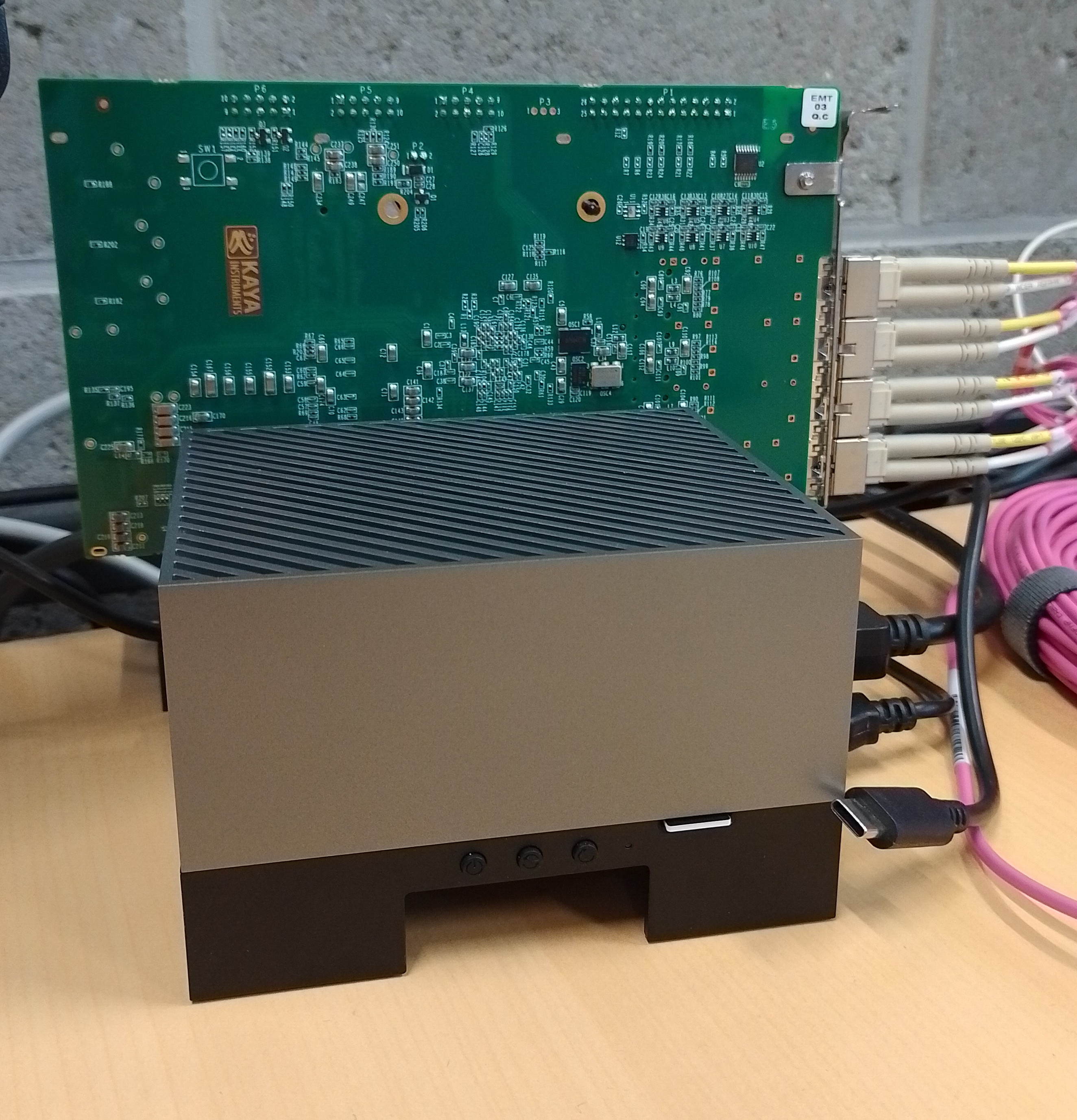
The embedded system of choice is an NVIDIA Jetson AGX Orin™ system, see Fig.˜1. This system is fairly powerful and expensive (2,000 EUR as of 03/2025) for an embedded device. The cost is, however, reasonable compared to the much more expensive metal printer and camera. The Jetson has an integrated 10 Gbps Ethernet \acNIC, a \acPCIe slot for hosting a frame grabber, and it can emulate smaller and cheaper devices of the same series. System and \acGPU memory are unified on the board. On the full AGX Orin, memory is not a constraining factor for storing the default \acNN architecture of the baseline model presented in this study. However, the speed of inference remains a constraint, as the system must be able to process the entire surface to catch all faults. The latency of this prediction should be low, i.e., feedback to the controller arrives within a few scanlines to avoid more damage and allow recovery of the fault. Ideally, this processing time should be not much longer than the time it takes to print a scanline.
The two objectives are therefore (i) inference speed and (ii) the \acRSME of the predictions. The inference speed for a model architecture is influenced by many factors, such as the number of parameters. It can be roughly estimated/interpolated (see Sec. 2), but only an execution on the device itself can reveal the true inference performance. Therefore, the inference speed of all model variants considered in this study are directly measured on the embedded device.
A central relational database (in PostgreSQL) has been set up to allow bi-directional communication between the embedded device located in Belgium at Flanders Make and the \acHPC cluster located at the Jülich Supercomputing Centre, Forschungszentrum Jülich, in Germany. The schema is shown in Fig.˜2.
The optimizer consults the embedded device as soon as it conceives a new candidate \acNN architecture (hyperparameter setting), posting the architecture details to the database. The embedded device continuously polls the database for unmeasured architectures, compiles and optimizes the architecture with the NVIDIA TensorRT library333NVIDIA TensorRT: https://developer.nvidia.com/tensorrt-getting-started, and (after warmup) runs a few inference steps to measure steady-state latency and throughput at several batch sizes. It subsequently reports its results back to the database.
The current setup lacks load balancing for multiple embedded devices of the same type, which is desirable for extremely large-scale optimizations, for efficient parallel operation also on the embedded side, as well as to achieve a degree of fault tolerance. At this point, further optimizations, such as the introduction of surrogate models, also become relevant.
3.1 Database Schema
The HPC2Edge database schema, shown in Fig. 2, consists of an essential part that supports basic communication between the \acHPC and edge systems (labeled ‘HPC2Edge core’ in the figure), and accessory tables to optionally store the full exploration of the optimizer.
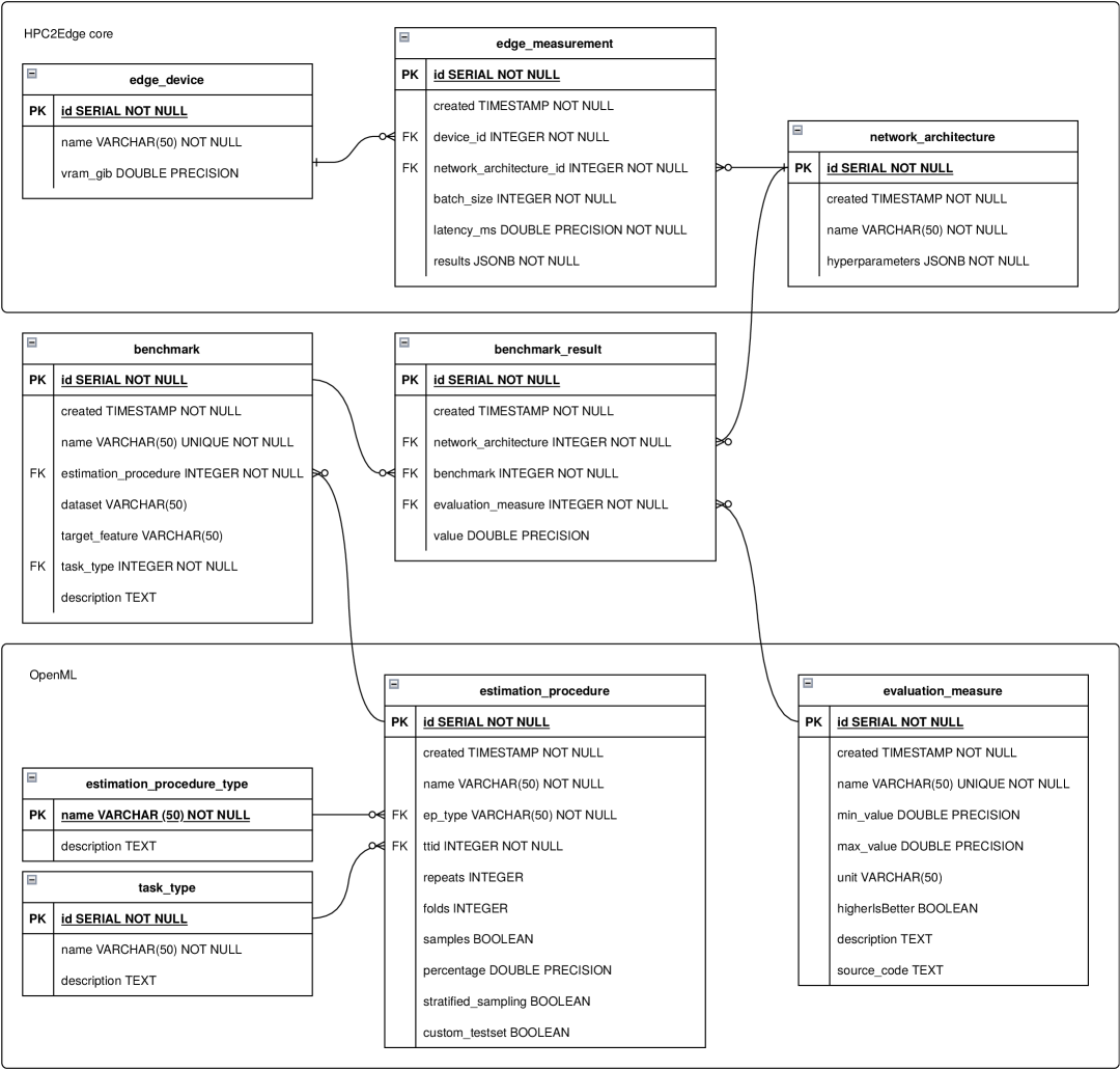
In terms of core schema, the edge device is GRANTed INSERT permission only into the edge_measurement table. The \acHPO algorithm gets an account that can INSERT into the (neural) network_architecture and benchmark_result tables. All accounts can SELECT from all tables. The JSONB columns allow noSQL-equivalent freedom to evolve the system without changing the main schema, but can still be indexed and efficiently queried when needed.
The extended schema is designed to be compatible with OpenML444OpenML: https://openml.org [13], which is an open platform for sharing datasets, algorithms, and experiments. OpenML has similarities to the more recent Hugging Face555Hugging Face: https://huggingface.co platform, it is, however, more geared towards classical \acML using tabular datasets. It offers \acpAPI and supports experiment logging from several popular \acML toolkits.
The present work uses the publicly available code as of 08/2024666OpenML 08/2024: https://github.com/openml/OpenML/tree/develop/data/sql.
Note that no full direct compatibility is achieved and OpenML has announced a full backend code rewrite, i.e., their future schema might be structured substantially different.
OpenML uses an extremely flexible, untyped schema. Here, some untyped, string-serialized fields were specialized to double precision, and the table math_function to estimation_procedure. Only reference records relevant for regression are stored, without loss of generality. The tables benchmark and benchmark_result correspond conceptually to tasks and runs in OpenML. It should be noted that the corresponding \acDDL was not available publicly to ensure some level of compatibility. Future work may consider running a full OpenML server for experiment logging — or some other logging method like MLflow 777MLflow: https://mlflow.org/ or ClearML 888ClearML: https://clear.ml/ — extended with only the HPC2Edge core schema.
3.2 AI Model
The model used to predict the laser parameters and to produce the following results (see Sec. 4) is a Video Swin Transformer [10] with a modified fully connected end layer for power and speed regression. The data pre-processing is the same as described in [2]. The RAISE-LPBF-Laser dataset (v1.1) [2], consisting of high-speed camera frames paired with various laser parameters, is used. Training and validation focus on a single object (C027) with an 80-20 split, while object C028 is used for testing. The proposed \acNAS framework directly optimizes performance for edge deployment, balancing both speed and accuracy, while leveraging \acHPC for acceleration. This work provides an efficient solution for real-time \acAI-driven industrial applications.
The input to the model consists of a window of consecutive frames that are randomly sampled from each scanline and then normalized and resized to a model input shape of pixels.
The output of the model corresponds to the ground-truth values, consisting of a pair of setpoints for laser dot speed and power for each scanline, which are normalized by dividing by their nominal values of 900 and 215, respectively. The choice of using a Video Swin model for prediction is motivated by the fact that it is the best performing attention-based model from [10] and that its architecture can be easily modified. Specifically, the model’s hyperparameters are well-designed to minimize conflicts and interdependencies, reducing the likelihood of parameterization issues during the optimization run.
The hyperparameters of the model that are optimized during the \acNAS run are listed in Tab. 1. The search space includes various Transformer-specific architectural parameters, i.e., the video patch size, which controls the temporal and spatial granularity of the input, the embedded dimensions influencing the dimensions of the tokens, the depths of each model stage, the number of attention heads, the window size of the self attention, and the ratio of feed-forward \acMLP layers between attention blocks. The classical optimizer-related parameters are the base learning rate of the Adam optimizer [7] and the scheduler-specific step-size and learning rate decay factor. The search space is chosen to be high-dimensional to allow for an extensive exploration of model size and model quality.
| Name | Description | Default | Sampling Range |
|---|---|---|---|
| Patch size | Video patch size for transformer tokenization | [2,4,4] | [2, 4] each |
| Embedded dimensions | Number of linear projection output channels | 96 | [24, 48] |
| Depths | Depths of each Video Swin Transformer stage | [2,2,6,2] | [1, 2, 4] each |
| Heads number | Number of attention heads of each stage | [3,6,12,24] | [3,6,12,24] each |
| \acMLP ratio | Ratio of \acMLP hidden dim. to embedding dim. | 4 | [1, 2, 3, 4] |
| Learning rate | Controls how much to adjust model weights during training | log[1e-5, 1] | |
| Learning rate step size | Interval of learning rate adjustment | 10 | [10, 20, 40] |
| Learning rate | Learning rate decay factor | 0.5 | (0.1, 0.9) |
3.3 Workflow Setup
The setup of the HPC2Edge workflow is shown in Fig. 3. The training of the different models is performed on the Extreme-Scale Booster partition of the DEEP-EST \acHPC machine [11] at the Jülich Supercomputing Centre, Forschungszentrum Jülich, in Germany. It features a total of 75 nodes, each one equipped with one NVIDIA V100 GPU and an Intel Xeon 4215 \acCPU with 8 cores and a base frequency of 2.5 GHz. To achieve results in a reasonable amount of time, the training of the different \acpNN is performed in data-parallel fashion with the PyTorch-DDP library999PyTorch-DDP: https://pytorch.org/docs/stable/notes/ddp.html. Orchestration of the \acHPO runs is handled by the Ray Tune framework101010Ray Tune: https://www.ray.io/. The optimization process leverages the Nevergrad library111111Nevergrad: https://facebookresearch.github.io/nevergrad/, a gradient-free optimization tool. Nevergrad performs evolutionary optimization in settings where the computation of gradients is hard or impossible. It is, therefore, a suitable solution for black box optimization problems such as \acHPO and \acNAS. It features a variety of optimization methods, that can be selected based on the search space and available computing budget. For the present work, the \acEA was chosen. The algorithm starts with an initial parent population and then creates one offspring for each parent via mutation. It subsequently evaluates the fitness of both the parent and the offspring. In case the offspring achieves a better fitness value than the parent, it replaces the parent in the subsequent generation. For the present experiments, the population size is fixed at , while the total number of evaluations is varied from to .
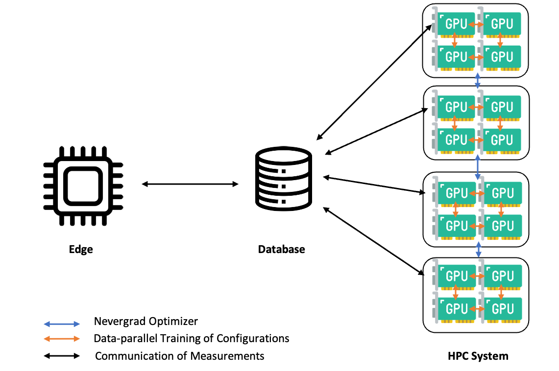
The edge device periodically queries the database for new, unevaluated entries that match its configuration, i.e., for supported edge device types. Upon finding a relevant entry, it loads the model parameters and performs ten inference runs to compute an average timing. This process is repeated for each configured batch size (1, 2, 4, and 8 in this case). The measured inference times, along with other measurements not exploited in this method, e.g., memory usage, \acCPU usage, or \acGPU usage, are entered in the database to be leveraged by the optimizer. Once a hyperparameter candidate is chosen, four \acpGPU are allocated to its training. With a population size of , this results in \acpGPU being used at the same time. Before launching the training, the head \acGPU submits the architectural details to the database for latency measurement on the edge device. After training for two epochs, the head node reads back this runtime measurement and combines it with the achieved validation loss. Submitting the architecture to the edge device before training the model and inquiring about the runtime measurement only after the model is trained hides the latency of communication between the \acHPC system and edge device.
| (1) |
A weighted validation score value, based on validation loss and inference time in milliseconds (see Eq. 1) is then reported back to the optimizer and minimized. The best performing model is chosen according to the lowest score achieved. This model is then evaluated on the unseen test dataset, where also a test score is computed in a similar way.
4 Empirical Results
The empirical results of running the hybrid workflow are shown in Tab. 2. It compares the default hyperparameter configuration, which was chosen by an expert (baseline) based on experience and several experiments, against running hardware-aware \acNAS with an increasing number of samples . The training times of a single configuration range between 1 – 3 hours, while the whole \acHPO run on the \acHPC system took between 8 – 19 hours, stretching the maximum allowed job time of 20 hours on the \acHPC system. The evaluation metrics include the validation loss , the inferences time and the test loss of the best configuration, which is chosen according to the lowest validation score metric , see Eq. (1). The most significant reduction in comparison to the baseline can be observed for the inference time metric. Using just samples decreases the inference time by a factor of from to . Increasing the number of samples to even leads to a reduction factor of in comparison to the baseline, which highlights the potential of the hybrid HPC2Edge workflow.
| Num. Samples | Val. Score | Val. Loss | Inference Time | Test Score | Test Loss |
|---|---|---|---|---|---|
| 0 (baseline) | 412.81 | 0.0807 | 457.51 | 0.1254 | |
| 16 | 146.02 | 0.0937 | 156.66 | 0.1044 | |
| 32 | 140.26 | 0.0959 | 140.53 | 0.0962 | |
| 64 | 129.99 | 0.0923 | 130.58 | 0.0929 |
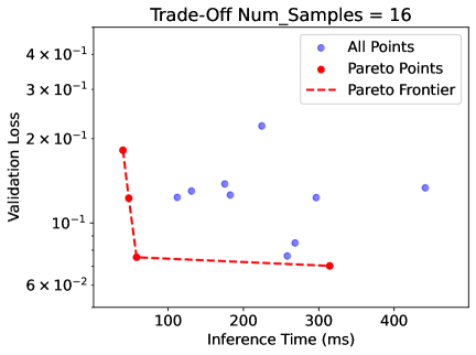
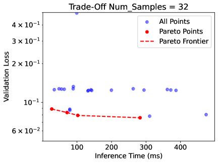
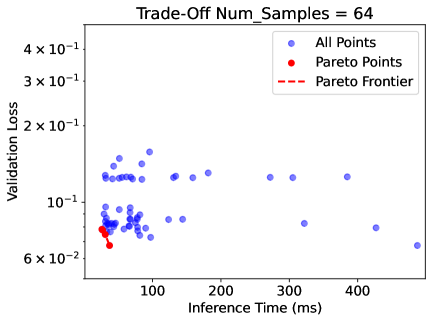
In terms of model quality, the validation loss metric shows varying performance across different sample sizes. At samples, the validation loss increases to , while at 64 samples it still remains higher at , compared to the baseline. In contrast, the samples \acNAS run results in the best model, decreasing the test loss by a factor of compared to the baseline model. It is hypothesized that the fluctuations in the validation loss metric are due to the weighting of both metrics into a single one, see Eq. (1), and thus a larger focus is on the inference time. However, as shown by the decreasing test loss, the model still seems to be able to achieve a higher solution quality than the baseline. Both metrics, the model quality on the test set and the inference time in general decrease for the model on the edge as the number of samples (and thus the compute resources spent on the \acNAS loop) is increased. In Fig. 4, the pareto curves of the different configurations are depicted, showing the optimal trade-off points between validation loss and inference time. As can be seen, in all cases the pareto curves do move to the left bottom of the plots, indicating better models.
To assess the importance of the architectural and optimizer-related parameters on the model performance, the top models found during the 5 \acNAS runs with samples are examined through their median hyperparameter values. The results show that a small learning rate of , combined with a large decay factor of and a moderate adjustment interval of steps results in the lowest validation score values. From an input data perspective, a median patch size of suggests larger patches to be more favorable. From an architectural point of view, a median depth of , a median attention head number of , and a median embedding dimension of suggests smaller models to be favorable. This is expected as these parameters usually also result in shorter inference times, which is one of the two objectives of the multi-objective optimizer.
5 Summary and Conclusion
In this work, a hybrid, cross-border, hardware-aware \acNAS workflow that runs in parallel on an \acHPC system and an edge device was presented. The workflow leverages the powerful \acpGPU of the \acHPC system to train different model configurations with data-parallel training while performing the inference time measurement of the models on the actual target device, resulting in an accurate measurement. To hide communication latency, each candidate model architecture is sent to the inference device before training on the \acHPC system. The empirical results clearly highlight how large savings in terms of inference time and model quality (in terms of final test loss) can be achieved. As a key finding, this research demonstrates empirically that increasing the computational resources of the \acHPO loop can lead to a smaller computational resource usage during the inference on the edge device. In the future, such workflows could therefore be used to find architectures with even higher speed (compared to expert baselines) or fitting on even smaller edge devices, which is an important feature not only in \acAM but in any field where fast \acML models are deployed on small devices.
5.0.1 Acknowledgements.
The CoE RAISE project has received funding from the European Union’s Horizon 2020 Research and Innovation Framework Programme H2020-INFRAEDI-2019-1 under grant agreement no. 951733. This research was also partially supported by the RELAI project of Flanders Make, the strategic research centre for the manufacturing industry, and by the Flemish Government AI Research Program. Resources for the database were provided by the VSC (Flemish Supercomputer Center), funded by the Research Foundation - Flanders (FWO) and the Flemish Government.
5.0.2 Disclosure of Interests.
The authors have no competing interests to declare that are relevant to the content of this article.
5.0.3 Venue and Manuscript Version.
This work was accepted for publication in the proceedings of ISC 2025 workshop Computational Aspects of Deep Learning (CADL 2025), and was selected for oral presentation. This preprint version of the manuscript, however, has not undergone peer review or any post-submission improvements or corrections. The Version of Record of this contribution will be published in HIGH PERFORMANCE COMPUTING: ISC High Performance 2025 International Workshops (Lecture Notes in Computer Science — LNCS).
References
- [1] Benmeziane, H., Maghraoui, K.E., Ouarnoughi, H., Niar, S., Wistuba, M., Wang, N.: A comprehensive survey on hardware-aware neural architecture search (2021), https://arxiv.org/abs/2101.09336
- [2] Blanc, C., Ahar, A., De Grave, K.: Reference dataset and benchmark for reconstructing laser parameters from on-axis video in powder bed fusion of bulk stainless steel. Additive Manufacturing Letters 7, 100161 (2023)
- [3] Booth, B.G., Heylen, R., Nourazar, M., Verhees, D., Philips, W., Bey-Temsamani, A.: Encoding stability into laser powder bed fusion monitoring using temporal features and pore density modelling. Sensors 22(10) (2022). https://doi.org/10.3390/s22103740
- [4] Eiben, A.E., Smith, J.E.: Introduction to Evolutionary Computing. Springer (2003)
- [5] Howard, A.G., Zhu, M., Chen, B., Kalenichenko, D., Wang, W., Weyand, T., Andreetto, M., Adam, H.: Mobilenets: Efficient convolutional neural networks for mobile vision applications (2017), https://arxiv.org/abs/1704.04861
- [6] Jiang, W., Zhang, X., Sha, E.H.M., Yang, L., Zhuge, Q., Shi, Y., Hu, J.: Accuracy vs. efficiency: Achieving both through FPGA-implementation aware neural architecture search. In: Proceedings of the 56th Annual Design Automation Conference 2019. DAC ’19, Association for Computing Machinery, New York, NY, USA (2019). https://doi.org/10.1145/3316781.3317757
- [7] Kingma, D.P., Ba, J.: Adam: A method for stochastic optimization. In: International Conference on Learning Representations (2015), http://arxiv.org/abs/1412.6980
- [8] Li, C., Yu, Z., Fu, Y., Zhang, Y., Zhao, Y., You, H., Yu, Q., Wang, Y., Lin, Y.C.: HW-NAS-bench: Hardware-aware neural architecture search benchmark. In: International Conference on Learning Representations (2021), https://openreview.net/forum?id=_0kaDkv3dVf
- [9] Lin, J., Chen, W.M., Lin, Y., Cohn, J., Gan, C., Han, S.: MCUNet: tiny deep learning on IoT devices. In: Proceedings of the 34th International Conference on Neural Information Processing Systems. NeurIPS ’20, Curran Associates Inc., Red Hook, NY, USA (2020)
- [10] Liu, Z., Ning, J., Cao, Y., Wei, Y., Zhang, Z., Lin, S., Hu, H.: Video swin transformer. In: Proceedings of the IEEE/CVF Conference on Computer Vision and Pattern Recognition (CVPR). pp. 3202–3211 (June 2022)
- [11] Suarez, E., Kreuzer, A., Eicker, N., Lippert, T.: The DEEP-EST project, Schriften des Forschungszentrums Jülich IAS Series, vol. 48, pp. 9–25. Forschungszentrum Jülich GmbH Zentralbibliothek, Verlag, Jülich (2021), https://juser.fz-juelich.de/record/905812
- [12] Sukthanker, R.S., Zela, A., Staffler, B., Klein, A., Purucker, L., Franke, J.K., Hutter, F.: HW-GPT-bench: Hardware-aware architecture benchmark for language models. In: The Thirty-eight Conference on Neural Information Processing Systems Datasets and Benchmarks Track (2024), https://openreview.net/forum?id=urJyyMKs7E
- [13] Vanschoren, J., van Rijn, J.N., Bischl, B., Torgo, L.: OpenML: networked science in machine learning. SIGKDD Explorations 15(2), 49–60 (2013). https://doi.org/10.1145/2641190.2641198
- [14] Wu, B., Keutzer, K., Dai, X., Zhang, P., Wang, Y., Sun, F., Wu, Y., Tian, Y., Vajda, P., Jia, Y.: Fbnet: Hardware-aware efficient convnet design via differentiable neural architecture search. In: 2019 IEEE/CVF Conference on Computer Vision and Pattern Recognition (CVPR). pp. 10726–10734. IEEE Computer Society, Los Alamitos, CA, USA (Jun 2019). https://doi.org/10.1109/CVPR.2019.01099
- [15] Zoph, B., Le, Q.: Neural architecture search with reinforcement learning. In: International Conference on Learning Representations (2017), https://openreview.net/forum?id=r1Ue8Hcxg