Robust feedback control of collisional plasma dynamics in presence of uncertainties

Abstract

Magnetic fusion aims to confine high-temperature plasma within a device, enabling the fusion of deuterium and tritium nuclei to release energy. Due to the very large temperatures involved, it is essential to isolate the plasma from the device walls to prevent structural damage and the external magnetic fields play a fundamental role in achieving this confinement. In realistic settings, the physical mechanisms governing plasma behavior are highly complex, involving numerous uncertain parameters and intricate particle interactions, such as collisions, that significantly affect both confinement efficiency and overall stability. In this work, we address particularly these challenges by proposing a robust feedback control strategy designed to steer the plasma towards a desired spatial region, despite the presence of uncertainties. From a modeling perspective, we consider a collisional plasma described by a Vlasov–Poisson–BGK system, which accounts for a self-consistent electric field and a strong external magnetic field, while incorporating uncertainty in the model. A key feature of the proposed control strategy is its independence from the random parameter, making it particularly suitable for practical applications. A series of numerical simulations confirms the effectiveness of our approach and demonstrates the ability of external magnetic fields to successfully confine plasma away from the device boundaries, even in the presence of uncertain conditions.

Keywords: Vlasov-Poisson system, collisional plasma, instantaneous control, magnetic confinement, uncertainty quantification, particle methods.
Mathematics Subject Classification: 35Q83, 82D10, 65C30, 35Q93, 65M75

1 Introduction

In recent years, considerable effort has been devoted to the development of advanced numerical methods aimed at addressing the complex challenges arising in plasma physics simulations [11, 19, 21, 33, 24]. A particular focus has been placed on the study of magnetized plasmas, due to their relevance in fusion energy applications, notably in confinement devices such as Tokamaks and Stellarators [47, 21, 48]. These devices rely on complex magnetic field configurations to confine and stabilize plasmas at very high temperatures. Reaching and maintaining optimal plasma conditions such as temperature, density, and confinement time is essential for the success of fusion experiments. However, the intrinsic complexity of plasma dynamics, characterized by turbulence, nonlinearity, and rapid transitions, combined with the influence of magnetic fields, poses important challenges both from the technical as well as from the simulation point of view [18, 20]. Addressing these issues demands the design and the use of new numerical schemes and multi-scale modeling strategies capable of accurately capturing the evolution of magnetized plasmas [4, 5, 12, 17, 10]. Additionally, the presence of uncertainty, ranging from limited knowledge of parameter settings, measurement errors in the magnetic field, the inability to define the exact initial configuration of the plasma, or the lack of accurate models to describe interactions with boundaries, to name a few, further complicates the analysis of the system. Nevertheless, such sources of uncertainty must be accounted for in the simulations [39, 40, 26, 27, 55, 54].

In this work, to describe the time evolution of the plasma flow under uncertain conditions, we consider a Vlasov–Poisson–BGK system, which models the dynamics of charged particles subject to a self-consistent electric field, an externally applied magnetic field, and collisional effects described through a relaxation toward thermodynamic equilibrium [46, 17, 16, 14, 49, 25]. Specifically, we focus on the time evolution of negatively charged particles, i.e. electrons, while we suppose the ions to constitute a fixed background. In this case, the governing equations read:

$$\begin{split}&\partial_{t}f(t,{\bf x},{\bf v},{\bf z})+{\bf v}\cdot\nabla_{\bf x}f(t,{\bf x},{\bf v},{\bf z})+\big{(}{\bf E}(t,{\bf x},{\bf z})+\\ &\qquad\qquad+{\bf v}\times{\bf B}_{ext}(t,{\bf x})\big{)}\cdot\nabla_{\bf v}f(t,{\bf x},{\bf v},{\bf z})=\frac{1}{\varepsilon}\mathcal{Q}(f(t,{\bf x},{\bf v},{\bf z})),\\ \vskip 5.69046pt&-\Delta_{\bf x}\phi(t,{\bf x},{\bf z})=\rho(t,{\bf x},{\bf z})-\rho_{i}(t,{\bf x},{\bf z}),\qquad{\bf E}(t,{\bf x},{\bf z})=-\nabla_{\bf x}\phi(t,{\bf x},{\bf z}),\end{split}$$ (1.1)

where the ions density is space homogeneous and immutable, i.e. $\rho_{i}(t,{\bf x},{\bf z})=1$, while the electrons density is defined by

$$\rho(t,{\bf x},{\bf z})=\int_{\mathbb{R}^{d_{v}}}f(t,{\bf x},{\bf v},{\bf z})\,d{\bf v},$$ (1.2)

with ${\bf z}\sim p({\bf z})$ a random variable modeling the uncertainty, distributed according to a known probability density function $p({\bf z})$. In this formulation, ${\bf E}(t,{\bf x},{\bf z})$, is the self-consistent electric field obtained from the Poisson equation (third line of (1.1)), ${\bf B}_{ext}(t,{\bf x})$ is an external magnetic field, assumed to be independent of the uncertainty. The collision operator $\mathcal{Q}(f)=\mu(M-f)$ is of relaxation type driving the distribution $f$ toward a local Maxwellian equilibrium $M(t,{\bf x},{\bf v},{\bf z})$ and with $\mu$ the collision frequency. The Vlasov equation (1.1) is written in adimensional form with $\varepsilon$ denoting the Knudsen number, which characterizes the relative importance of collisional effects, the Debye length is chosen equal to one in the Poisson equation and thus omitted.

The above depicted dynamics, in the deterministic case, can be approximated by means of different numerical schemes ranging from finite difference, finite volume to semilagrangian methods [47, 15, 17, 18, 21, 45, 53, 19]. Uncertainty for the Vlasov equation has been considered for instance in [55, 36, 39]. In this paper, we focus on Particle-In-Cell (PIC) schemes [6, 22, 50, 49, 2] with the aim of designing specific control strategies in the presence of uncertainties which in turns will be handled through stochastic collocation (SC) methods [52]. In PIC simulations, the plasma is represented by a large number of particles that carry physical quantities such as electric charge and mass. These particles move through a computational grid where the electromagnetic fields are solved, [31, 32, 33, 34]. To tackle the presence of uncertainty, we introduce Gauss-Legendre nodes and use quadrature formulas [52] to compute different quantity of interests such as the expectation and the variance with respect to the uncertain space. In addition, robust optimization techniques are used to formulate an optimal control problem that accounts for uncertainties [1]. Specifically, the goal is to design control strategies that optimize the magnetic field configuration to achieve desired plasma parameters while accounting for the variability in the system. More in details, the control problem we aim to study is given by

$$\min_{{\bf B}_{ext}\in\mathcal{B}^{adm}}\mathcal{J}({\bf B}_{ext};f^{0};f),\qquad\textrm{subject to }\quad\eqref{eq:vlasov_poisson},$$ (1.3)

where $\mathcal{B}^{adm}$ is a set of admissible controls, $f^{0}$ the initial datum, and $\mathcal{J}(\cdot)$ is a functional which reads as follows

$$\mathcal{J}({\bf B}_{ext};f^{0};f)= \int_{0}^{t_{f}}\left(\mathcal{P}[\mathcal{D}(f,\psi)(t,{\bf z})]+\right.$$ (1.4)

$$\left.+\frac{\gamma}{2}\mathcal{P}\Big{[}\int_{\Omega}|{\bf B}_{ext}(t,{\bf x})|^{2}f(t,{\bf x},{\bf v},{\bf z})d{\bf x}d{\bf v}\Big{]}\right)dt$$

where

$$\mathcal{D}(f,\psi)(t,{\bf z})=\int_{\Omega}\psi({\bf x},{\bf v},{\bf z})\left(f(t,{\bf x},{\bf v},{\bf z})-\hat{f}(t,{\bf x},{\bf v})\right)d{\bf x}d{\bf v},$$ (1.5)

is a running cost function, being $\hat{f}$ a given target distribution discussed next, $\psi({\bf x},{\bf v},{\bf z})$ a function of the state variables, $\mathcal{P}(\cdot)$ a statistical operator counting for the uncertainties, $\Omega=\Omega_{x}\times\Omega_{v}$, $t_{f}$ a final prescribed time, and $\gamma$ a weight penalizing the magnitude of the control given by the external magnetic field ${\bf B}_{ext}$. The scope of the functional in (1.4) is to force the distribution function or its moments towards desired values through the choice of the function $\psi({\bf x},{\bf v},{\bf z})$. Similar problems have been investigated from an analytical perspective in recent literature, in the absence of collisions and uncertainties, see, for example, [8, 37]. From a numerical standpoint, related approaches have also been explored in [3, 30, 2, 29]. In particular, in [2] the authors of the present article, introduced a piecewise spatial control strategy based on the external magnetic field to confine a plasma governed by the Vlasov–Poisson model. The control targeted both the position and velocity of charged particles and was modeled as spatially constant but time-dependent, applied over a finite set of spatial cells. This setup reflects a physically realistic configuration, in which arbitrarily localized magnetic field values are not admissible. To design an effective instantaneous control strategy, all these constraints were explicitly incorporated into the control functional (see Appendix A for further details).

The main objective of this work is to extend the results of [2] and to develop a new optimal instantaneous control strategy in the presence of uncertainty. To the best of our knowledge, this is the first study addressing the control of out-of-equilibrium plasmas characterized by uncertain parameters. In greater detail, as opposite from [2], we first derive a pointwise instantaneous control that acts individually on each particle. Building on this fine-scale information, we then construct a coarse-grained control by averaging the local control fields obtained from the minimization procedure. This yields a piecewise constant-in-space, time-dependent magnetic control field, designed to approximate the effect of the optimal microscopic control over a realistic spatial configuration and in the presence of uncertainties. We demonstrate that this approach allows for effective steering of the plasma toward desired configurations, without requiring highly complex magnetic field structures.

The remainder of the paper is organized as follows. In Section 2.1, we formulate the control problem within a two-dimensional setting, presenting its general structure and the modeling framework adopted. In Section 2.2, we introduce the numerical methods used to solve the Vlasov–Poisson system under uncertainty, with particular emphasis on Particle-In-Cell schemes and the Gauss–Legendre quadrature for handling stochastic parameters. In Section 3, we discretize the control problem and derive a strategy capable of managing both uncertainty and collisional effects. Section 4 presents a series of numerical experiments that validate the effectiveness of the proposed method. In Section 5, we summarize the main results and outline possible directions for future work. Finally, the appendix A is devoted to the extension of the control strategy proposed in [2] to the setting with uncertainty, and to a comparison with the new approach developed in this work, highlighting the improvements and the enhanced performance achieved by the latter.

2 Problem setting and numerical methods

In the remainder of the work, we restrict our analysis to a two-dimensional phase space setting, which serves as a simplified model for the evolution of plasma within a three-dimensional axisymmetric toroidal configuration. In this section, we first discuss the setting and then we propose a suitable numerical discretization for the Vlasov–Poisson–BGK model with uncertainties. In the following section, based on the discussed discretization, we introduce and study an instantaneous control strategy.

2.1 Control of the Vlasov–Poisson–BGK model with uncertainties

In the proposed configuration, the reference frame $({\bf x}_{\perp},{\bf v}_{\perp})$ is chosen such that the external magnetic field remains always orthogonal to the plane in which the time evolution of the single-species plasma distribution function takes place. This gives

$$f=f(t,{\bf x}_{\perp},{\bf v}_{\perp},{\bf z}),\qquad f:\mathbb{R}_{+}\times\Omega_{x}\times\Omega_{v}\times\Omega_{z},$$ (2.1)

where $\Omega_{z}\subseteq\mathbb{R}^{d_{z}}$ denotes the uncertainty space, $\Omega_{x}\subseteq\mathbb{R}^{d_{x}}$, $\Omega_{v}\subseteq\mathbb{R}^{d_{v}}$ the space and velocity domain, and where we set from now on $d_{x}=d_{v}=2$. The evolution of $f(t,{\bf x}_{\perp},{\bf v}_{\perp},{\bf z})$ is then governed by the following collisional Vlasov-type equation

$$\begin{split}&\partial_{t}f+{\bf v}_{\perp}\cdot\nabla_{{\bf x}_{\perp}}f+F(t,{\bf x}_{\perp},{\bf v}_{\perp},{\bf z})\cdot\nabla_{{\bf v}_{\perp}}f=\frac{1}{\varepsilon}\mathcal{Q}(f),\\ &f(0,{\bf x}_{\perp},{\bf v}_{\perp},{\bf z})=f_{0}({\bf x}_{\perp},{\bf v}_{\perp},{\bf z}),\end{split}$$ (2.2)

where $f_{0}$ denotes the initial distribution function, which depends on the uncertain parameter ${\bf z}$, assumed to follow a given probability distribution $p({\bf z})$. For brevity, we omitted the explicit dependence of $f$ on $t,{\bf x}_{\perp},{\bf v}_{\perp}$, and ${\bf z}$ in previous expression (2.2). The force field acting on the particles is given by:

$$F(t,{\bf x}_{\perp},{\bf v}_{\perp},{\bf z})={\bf E}(t,{\bf x}_{\perp},{\bf z})+{\bf v}_{\perp}\times{\bf B}_{ext}(t,{\bf x}_{\perp}),$$ (2.3)

where ${\bf B}_{ext}$ is the external magnetic field, assumed to be independent of the uncertainty ${\bf z}$ as already stated, and ${\bf E}$ is the electric field derived from the solution of the Poisson equation:

$${\bf E}(t,{\bf x}_{\perp},{\bf z})=-\nabla_{{\bf x}_{\perp}}\phi(t,{\bf x}_{\perp},{\bf z}),\qquad-\Delta_{{\bf x}_{\perp}}\phi(t,{\bf x}_{\perp},{\bf z})=\rho(t,{\bf x}_{\perp},{\bf z})-1,$$ (2.4)

with $\phi$ the electric potential, and the charge density defined as:

$$\rho(t,{\bf x}_{\perp},{\bf z})=\int_{\Omega_{v}}f(t,{\bf x}_{\perp},{\bf v}_{\perp},{\bf z})\,d{\bf v}_{\perp}.$$ (2.5)

The right-hand side of equation (2.2), $\mathcal{Q}(f)$, describes the collisions among particles. In this work, we adopt a BGK-type operator defined as:

$$\mathcal{Q}(f)=\mu\left(\mathcal{M}(t,{\bf x}_{\perp},{\bf v}_{\perp},{\bf z})-f(t,{\bf x}_{\perp},{\bf v}_{\perp},{\bf z})\right),$$ (2.6)

where $\mu$ is the collision frequency which in general may depend upon the macroscopic quantities and the uncertain parameters, i.e. $\mu=\mu(\rho,T,{\bf z})$, and $\mathcal{M}$ is the local Maxwellian equilibrium distribution given by:

$$\mathcal{M}(t,{\bf x}_{\perp},{\bf v}_{\perp},{\bf z})=\frac{\rho(t,{\bf x}_{\perp},{\bf z})}{2\pi T(t,{\bf x}_{\perp},{\bf z})}\exp\left(-\frac{|{\bf v}_{\perp}-{\bf U}(t,{\bf x}_{\perp},{\bf z})|^{2}}{2T(t,{\bf x}_{\perp},{\bf z})}\right),$$ (2.7)

with ${\bf U}$, and $T$ denoting the mean velocity and temperature, respectively, computed as:

$$\begin{split}{\bf U}(t,{\bf x}_{\perp},{\bf z})&=\frac{1}{\rho(t,{\bf x}_{\perp},{\bf z})}\int_{\Omega_{v}}{\bf v}_{\perp}f(t,{\bf x}_{\perp},{\bf v}_{\perp},{\bf z})\,d{\bf v}_{\perp},\\ T(t,{\bf x}_{\perp},{\bf z})&=\frac{1}{2\rho(t,{\bf x}_{\perp},{\bf z})}\int_{\Omega_{v}}|{\bf v}_{\perp}-{\bf U}(t,{\bf x}_{\perp},{\bf z})|^{2}f(t,{\bf x}_{\perp},{\bf v}_{\perp},{\bf z})\,d{\bf v}_{\perp}.\end{split}$$ (2.8)

The final scope is to control the dynamics described by (2.2)-(2.4) using an external magnetic field to configure charged particles into a desired setting while keep them as far as possible from the walls. To achieve this, we start from the following continuous control problem

$$\min_{{\bf B}^{ext}\in\mathcal{B}_{adm}}\mathcal{J}({\bf B}_{ext};f^{0},f),\qquad\textrm{s.t.}\leavevmode\nobreak\ \eqref{eq:Vlasov}-\eqref{eq:Poisson}\ \text{are satisfied}$$ (2.9)

where

$$\begin{split}&\mathcal{J}({\bf B}_{ext};f^{0},f)=\int_{0}^{t_{f}}\mathcal{P}\ \left[\sum_{\ell\in\{\text{x},\text{v}\}}\mathcal{D}(f,\psi_{\ell})(t,{\bf z})\right]dt+\cr&\qquad+\frac{\gamma}{2}\int_{0}^{t_{f}}\mathcal{P}\left[\int_{\Omega}|{\bf B}_{ext}(t,{\bf x}_{\perp})|^{2}f(t,{\bf x}_{\perp},{\bf v}_{\perp},{\bf z})d{\bf x}_{\perp}d{\bf v}_{\perp}\right]dt,\end{split}$$ (2.10)

with $\Omega=\Omega_{x}\times\Omega_{v}$, and where $\mathcal{D}(\cdot)$ aims at enforcing a specific configuration of the distribution function and of its moments, that is

$$\begin{split}\mathcal{D}(f,\psi_{\ell})(t,{\bf z})=&\frac{\alpha_{\ell}}{2}|m(f,\psi_{\ell})(t,{\bf z})-\hat{\psi}_{\ell}|^{2}+\frac{\beta_{\ell}}{2}m_{\sigma}(f,\psi_{\ell})(t,{\bf z}),\end{split}$$ (2.11)

with $\alpha_{\ell},\beta_{\ell}\geq 0$ weighting parameters for $\ell=\{\text{x},\text{v}\}$, and

$$\begin{split}&m(f,\psi_{\ell})(t,{\bf z})=\int_{\Omega}\psi_{\ell}({\bf x}_{\perp},{\bf v}_{\perp},{\bf z})f(t,{\bf x}_{\perp},{\bf v}_{\perp},{\bf z})d{\bf x}_{\perp}d{\bf v}_{\perp},\\ &m_{\sigma}(f,\psi_{\ell})(t,{\bf z})=\int_{\Omega}|\psi_{\ell}({\bf x}_{\perp},{\bf v}_{\perp},{\bf z})-m(f,\psi_{\ell})(t,{\bf z})|^{2}f(t,{\bf x}_{\perp},{\bf v}_{\perp},{\bf z})d{\bf x}_{\perp}d{\bf v}_{\perp}.\end{split}$$ (2.12)

The first equation in (2.12) aims at enforcing the moments of the distribution function to assume some given values in different regions of the physical space through concentration of the distribution function at some given target $\hat{\psi}_{\ell}$. The second equation tries to minimizes the distance from the average value $m(f,\psi_{\ell})$ both in space as well as in velocity space around these targets.

The statistical operator $\mathcal{P}[\cdot]$ is introduced to ensure the robustness of the control strategy with respect to the uncertainty parameter ${\bf z}$. One natural choice for $\mathcal{P}[\cdot]$ is the mathematical expectation in the random space, defined as:

$$\mathcal{P}[\varphi_{f}(\cdot,{\bf z})]=\int_{\Omega_{z}}\varphi_{f}(\cdot,{\bf z})\,p({\bf z})\,d{\bf z},$$ (2.13)

where $\varphi_{f}(\cdot,{\bf z})$ is a measurable quantity depending on the uncertainty ${\bf z}$. An alternative measure of robustness that we consider in this work is based on the worst-case scenario idea, which corresponds to minimizing a given macroscopic quantity related to the plasma evolution over all admissible realizations of ${\bf z}$. In this case, the operator takes the form:

$$\mathcal{P}[\varphi_{f}(\cdot,{\bf z})]=\varphi_{f}(\cdot,{\bf z}_{0}),\qquad\text{with }\leavevmode\nobreak\ {\bf z}_{0}=\arg\max_{\bf z}T_{b}(\cdot,{\bf z}),$$ (2.14)

being $T_{b}(\cdot,{\bf z})$ the temperature close to the boundary for a fixed value of the uncertainty.

2.2 A stochastic collocation particle-MC method

We focus now on the numerical solution of the Vlasov equation (2.2) in the presence of uncertainty. The proposed numerical approach combines Particle-In-Cell (PIC) techniques for the transport part [9, 31] with Direct Simulation Monte Carlo (DSMC) methods to handle the collisional term [43, 44, 6, 23]. To incorporate uncertainty, several strategies have been proposed in the literature about Vlasov or related kinetic type equations with random inputs, ranging from intrusive Stochastic Galerkin methods [35, 13, 51, 28] to non-intrusive techniques such as Monte Carlo sampling [26, 27, 38]. In this work we focus on an alternative non-intrusive approach: the stochastic collocation (SC) method [52, 41] which up to our knowledge it has never been used for treating uncertainties in the context of Vlasov-type equations.

For a quantity of interest $\varphi_{f}(t,{\bf x}_{\perp},{\bf v}_{\perp},{\bf z})$, we first define its expected value and variance in the uncertain space as:

$$\mathbb{E}[\varphi_{f}](t,{\bf x}_{\perp},{\bf v}_{\perp})=\int_{\Omega_{z}}\varphi_{f}(t,{\bf x}_{\perp},{\bf v}_{\perp},{\bf z})p({\bf z})\,d{\bf z},$$ (2.15)

$$\sigma^{2}[\varphi_{f}](t,{\bf x}_{\perp},{\bf v}_{\perp})=\int_{\Omega_{z}}\left(\varphi_{f}(t,{\bf x}_{\perp},{\bf v}_{\perp},{\bf z})-\mathbb{E}[\varphi_{f}](t,{\bf x}_{\perp},{\bf v}_{\perp})\right)^{2}p({\bf z})\,d{\bf z}.$$ (2.16)

Additional observable can be defined in the same manner. Typical quantities of interest include the distribution function $f$ itself, as well as its moments: density, mean velocity, and temperature for example. In the latter cases, the dependence on ${\bf v}_{\perp}$ is dropped in (2.15)-(2.16). We then select $N_{z}$ quadrature nodes $\{z_{k}\}_{k=1}^{N_{z}}$ (where we suppose to use only one index to describe the multidimensional space $\Omega_{z}$) with corresponding weights $\{w_{k}\}$ for a given quadrature rule adapted to the distribution $p({\bf z})$ and solve $N_{z}$ independent deterministic Vlasov problems. We also suppose, to easily describe the proposed approach, that uncertainty affects only the initial data, i.e. $f_{0}({\bf x}_{\perp},{\bf v}_{\perp},{\bf z})$. For each node we have then:

$$\partial_{t}f^{k}(t,{\bf x}_{\perp},{\bf v}_{\perp})+{\bf v}_{\perp}\cdot\nabla_{{\bf x}_{\perp}}f^{k}+F^{k}(t,{\bf x}_{\perp},{\bf v}_{\perp})\cdot\nabla_{v_{\perp}}f^{k}=\frac{1}{\varepsilon}\mathcal{Q}(f^{k}),$$ (2.17)

being $F^{k}(t,{\bf x}_{\perp},{\bf v}_{\perp})=({\bf E}^{k}(t,{\bf x}_{\perp})+{\bf v}_{\perp}\times{\bf B}_{ext}(t,{\bf x}_{\perp}))$, with initial data $f_{0}^{k}=f_{0}(\cdot,\cdot,z_{k})$. The SC method to approximate expected value and variance in the uncertain space is then obtained by the following algorithm:

Algorithm 2.1 (Stochastic collocation for the Vlasov equation with random inputs).

1. Consider $N_{z}$ collocation nodes $z_{k}$ and weights $w_{k}$ using Gauss quadrature according to $p({\bf z})$.

2. For each node $z_{k}$, solve the deterministic Vlasov problem with the preferred numerical technique to get $\tilde{f}^{k,n}$.

3. Compute the expected value and variance of the quantity of interest. For example in the case of the computation of expectation and variance for the distribution function, one has

   $$E_{N_{z}}[\tilde{f}^{n}]=\sum_{k=1}^{N_{z}}w_{k}\tilde{f}^{n,k},\quad\sigma^{2}_{N_{z}}[\tilde{f}^{n}]=\sum_{k=1}^{N_{z}}w_{k}\left(\tilde{f}^{n,k}-E_{N_{z}}[\tilde{f}^{n}]\right)^{2}.$$

   Other statistics with respect the random space and related to the distribution function or its moments can be computed in the same manner.

This method benefits from spectral convergence when the solution depends smoothly on the uncertain parameter ${\bf z}$, i.e., the error decays faster than any power of $N_{z}^{-1}$, depending on regularity of the solution. The typical error estimate reads, in the case in which the other discretization errors are neglected, as:

$$|\mathbb{E}[f]-E_{N_{z}}[\tilde{f}])|\leq Cp^{-2N_{z}}$$

with $C$ and $p$ two constants.

In order to approximate the $N_{z}$ deterministic collisional Vlasov equations (2.17), we rely on a particle method. This approach consists first in approximating the initial condition $f_{0}({\bf x}_{\perp},{\bf v}_{\perp})$ in (2.17) by a discrete sum of Dirac masses (we omit from now on the apex $k$ indicating the point in the random space):

$$f_{N}^{0}({\bf x}_{\perp},\mathbf{v}_{\perp}):=\sum_{m=1}^{N}\omega_{m}\delta\left(\mathbf{x}_{\perp}-\mathbf{x}_{m}^{0}\right)\delta\left(\mathbf{v}_{\perp}-\mathbf{v}_{m}^{0}\right),$$ (2.18)

where $\left(\mathbf{x}_{m}^{0},\mathbf{v}_{m}^{0}\right)_{1\leq m\leq N}$ represent the initial positions and velocities of the particles, and $\omega_{m}$ are the associated particle weights. Next, we introduce a spatial discretization grid composed of $M_{c}$ cells $\mathcal{C}_{j}$, $j=1,\ldots,M_{c}$, used to compute the electric field, together with a time discretization of the interval $[0,t_{f}]$ with step size $h>0$. In this setting, the approximate solution of the Vlasov equation at time level $n$ is given by:

$$f_{N}^{n}({\bf x}_{\perp},{\bf v}_{\perp})=\sum_{m=1}^{N}\omega_{m}\delta({\bf x}_{\perp}-{\bf x}_{m}^{n})\delta({\bf v}_{\perp}-{\bf v}_{m}^{n}),$$ (2.19)

where the particle positions and velocities at time level $n$ are updated through a splitting procedure between the collision and transport steps.

The collision step is defined by:

$$\begin{cases}\partial_{t}f_{N}^{*}=\dfrac{1}{\varepsilon}\mathcal{Q}(f_{N}^{*}),\\ f_{N}^{*}(0,{\bf x}_{\perp},{\bf v}_{\perp})=f_{N}^{n}({\bf x}_{\perp},{\bf v}_{\perp}),\end{cases}$$ (2.20)

while the transport step is given by:

$$\begin{cases}\partial_{t}f_{N}^{**}+{\bf v}_{\perp}\cdot\nabla_{{\bf x}_{\perp}}f_{N}^{**}+({\bf E}^{**}+{\bf v}_{\perp}\times{\bf B}_{ext}^{**})\cdot\nabla_{{\bf v}_{\perp}}f_{N}^{**}=0,\\ f_{N}^{**}(0,{\bf x}_{\perp},{\bf v}_{\perp})=f_{N}^{*}({\bf x}_{\perp},{\bf v}_{\perp}),\end{cases}$$ (2.21)

thus yielding the solution at time $t^{n+1}$:

$$f_{N}^{n+1}({\bf x}_{\perp},{\bf v}_{\perp})=\mathcal{T}_{h}\left(\mathcal{Q}_{h}(f_{N}^{n})({\bf x}_{\perp},{\bf v}_{\perp})\right).$$

The discretization of the collision step gives:

$$f_{N}^{*}({\bf x}_{\perp},{\bf v}_{\perp})=e^{-\nu h}f_{N}^{n}({\bf x}_{\perp},{\bf v}_{\perp})+(1-e^{-\nu h})\mathcal{M}_{N}^{n}({\bf x}_{\perp},{\bf v}_{\perp}),$$ (2.22)

where $\nu=\mu/\varepsilon$ and $\mathcal{M}_{N}^{n}(\cdot)$ is the local Maxwellian distribution (2.7) computed from the knowledge of the moments of $f$ and ^∗ indicates that (2.22) furnishes the solution of the sole collisional part (2.20) which will be then used as an initial data for the solution of the Vlasov equation (2.21). It is important to observe that the collisional term modifies only the particle velocities, while preserving the first three moments of $f$, namely mass, momentum, and energy. This means that $\mathcal{M}$ is constant over the relaxation step (2.21). From a probabilistic viewpoint, relation (2.22) is interpreted as follows [42, 7]: with probability $e^{-\nu h}$, the velocity ${\bf v}_{m}$ of a particle remains unchanged, while with probability $1-e^{-\nu h}$, it is replaced by a velocity sampled from the local Maxwellian. This can be expressed as:

$${\bf v}_{m}^{*}=\chi(\eta_{m}<e^{-\nu h}){\bf v}_{m}^{n}+(1-\chi(\eta_{m}<e^{-\nu h}))\left({\bf U}_{m}^{n}+\xi_{m}\sqrt{T_{m}^{n}}\right),$$ (2.23)

where $\eta_{m}\sim\mathcal{U}([0,1])$ is uniformly distributed, $\xi_{m}\sim\mathcal{N}(0,1)$ is a standard normal random variable, and $\chi(\cdot)$ denotes the indicator function. Here, ${\bf U}_{m}^{n}$ and $T_{m}^{n}$ are defined as:

$${\bf U}_{m}^{n}=\sum_{j=1}^{M_{c}}\tilde{{\bf U}}_{j}^{n}\chi({\bf x}^{n}_{m}\in\mathcal{C}_{j}),\qquad T_{m}^{n}=\sum_{j=1}^{M_{c}}\tilde{T}_{j}^{n}\chi({\bf x}^{n}_{m}\in\mathcal{C}_{j}),$$

where:

$$\begin{split}\tilde{{\bf U}}_{j}^{n}&=\dfrac{1}{\tilde{\rho}_{j}^{n}}\sum_{m=1}^{N}\omega_{m}{\bf v}_{m}^{n}\chi({\bf x}_{m}^{n}\in\mathcal{C}_{j}),\\ \tilde{T}_{j}^{n}&=\dfrac{1}{2\tilde{\rho}_{j}^{n}}\sum_{m=1}^{N}\omega_{m}|{\bf v}_{m}^{n}-\tilde{{\bf U}}_{j}^{n}|^{2}\chi({\bf x}_{m}^{n}\in\mathcal{C}_{j}),\end{split}$$ (2.24)

represent the local momentum and temperature at time $t^{n}$ within cell $\mathcal{C}_{j}$, and

$$\tilde{\rho}_{j}^{n}=\sum_{m=1}^{N}\omega_{m}\chi({\bf x}_{m}^{n}\in\mathcal{C}_{j})$$

is the local particle density.

The transport phase in phase space is finally recovered by approximating the particle trajectories according to the characteristic curves of the Vlasov equation:

$$\begin{split}\frac{d{\bf x}_{m}(t)}{dt}&={\bf v}_{m}(t),\\ \frac{d{\bf v}_{m}(t)}{dt}&={\bf E}(t,{\bf x}_{m})+{\bf v}_{m}\times{\bf B}_{ext}(t,{\bf x}_{m}).\end{split}$$ (2.25)

Here, the electric field ${\bf E}(t,{\bf x})$ is obtained by approximating the Poisson equation with a finite difference method on the spatial grid. Then the value of ${\bf E}$ at the particle position ${\bf x}_{m}$ is taken as the value at the center of the cell $\mathcal{C}_{j}$ containing ${\bf x}_{m}$. At each time step, the approximated density, needed to solve the Poisson equation, is reconstructed over the spatial cells $\mathcal{C}_{j}$ from the updated particle positions and velocities. To discretize (2.25), we use a semi-implicit first-order scheme [31]:

$$\begin{split}{\bf x}_{m}^{n+1}&={\bf x}_{m}^{n}+h{\bf v}_{m}^{n+1},\\ {\bf v}_{m}^{n+1}&={\bf v}_{m}^{*}+h\left({\bf v}_{m}^{n+1}\times{\bf B}_{ext}(t^{n},{\bf x}_{m}^{n})+{\bf E}(t^{n},{\bf x}_{m}^{n})\right),\end{split}$$ (2.26)

where ${\bf B}_{ext}(t^{n},{\bf x}_{m}^{n})$ denotes the external magnetic field computed at the particle location, which will be determined in the control problem discussed in the next Section 3. In the rest of the paper we will drop for simplicity the _⟂ in the notation and consequently we will write ${\bf x}$ instead of ${\bf x}_{\perp}$ and ${\bf v}$ instead of ${\bf v}_{\perp}$.

3 Robust feedback control by an external magnetic field

We now describe the robust feedback control strategy for the uncertain Vlasov–Poisson–BGK system introduced in Section 2.1. We begin our analysis by computing the external magnetic field ${\bf B}_{\text{ext}}$ which is, by hypothesis orthogonal to the plane identified by ${\bf x}$ and consequently we set ${\bf B}_{\text{ext}}=(0,0,B)$.

We discretize the time interval $[0,t_{f}]$ into subintervals of length $h$, and solving the following sequence of instantaneous optimal control problems:

$$\begin{split}&\min_{B\in\mathcal{B}_{adm}}\mathcal{J}(B;f_{N}^{0},f_{N}):=\int_{t}^{t+h}\mathcal{P}\left[\sum_{\ell\in\{\text{x},\text{v}\}}\mathcal{D}(f_{N},\psi_{\ell})(\tau,{\bf z})\right]d\tau+\\ &\qquad\qquad\quad+\frac{\gamma}{2}\int_{t}^{t+h}\mathcal{P}\left[\int_{\Omega}|B(\tau,{\bf x})|^{2}f_{N}(\tau,{\bf x},{\bf v},{\bf z})d{\bf x}d{\bf v}\right]d\tau,\end{split}$$ (3.1)

where $\mathcal{P}$ is defined as in (2.13)–(2.14), and ${B}_{adm}=\{B|B\in[-M,M],M>0\}$, with $M$ denoting the maximum admissible magnetic field strength. The function $\mathcal{D}(f_{N},\psi_{\ell})(\tau,{\bf z})$ is defined in (2.11), and $f_{N}$ denotes the empirical density.

Applying a semi-implicit rectangle rule to approximate the time integrals in (3.1), we obtain the discrete cost functional (3.1) as follows

$$\mathcal{J}^{h}(B;f_{N}^{0},f_{N}) =h\mathcal{P}\left[\sum_{\ell\in\{\text{x},\text{v}\}}\mathcal{D}(f^{n+1}_{N},\psi_{\ell})(\tau,{\bf z})\right]+$$ (3.2)

$$+\frac{h\gamma}{2}\mathcal{P}\left[\int_{\Omega}|B^{n+1}({\bf x})|^{2}f_{N}^{n+1}({\bf x},{\bf v},{\bf z})d{\bf x}d{\bf v}\right].$$

3.1 Derivation of an approximated feedback control

Our next goal is to insert the explicit form of the empirical distribution into (3.2), under the constraint of the semi-implicit dynamics (2.22)–(2.26). However, this would prevent an explicit computation of the optimal magnetic field.

To overcome this issue, we introduce a simplified time integrator that replaces the semi-implicit scheme used in the evolution of the plasma dynamics. While the original scheme is well suited for accurate simulation, it leads to a highly coupled optimality system that is not tractable for instantaneous control synthesis. The simplified integrator decouples the forward dynamics and allows for a closed-form expression of the optimal magnetic field at each particle location. Although this comes at the cost of an approximation, it enables the construction of an efficient and interpretable feedback strategy that can later be embedded into the full semi-implicit dynamics.

To this aim, we replace the numerical scheme (2.22)–(2.26) with the modified semi-implicit scheme:

$$\begin{split}&x_{m}^{n+1}({\bf z})=x_{m}^{n}({\bf z})+hv_{x_{m}}^{n+1}({\bf z}),\\ &y_{m}^{n+1}({\bf z})=y_{m}^{n}({\bf z})+hv_{y_{m}}^{n+1}({\bf z}),\\ &v_{x_{m}}^{n+1}({\bf z})=v_{x_{m}}^{*}({\bf z})+hv_{y_{m}}^{*}({\bf z})B^{n+1}_{m}+hE_{x_{m}}^{n}({\bf z}),\\ &v_{y_{m}}^{n+1}({\bf z})=v_{y_{m}}^{*}({\bf z})-hv_{x_{m}}^{*}({\bf z})B^{n+1}_{m}+hE_{y_{m}}^{n}({\bf z}),\\ &v_{x_{m}}^{*}({\bf z})=\theta_{m}^{\nu,h}v_{x_{m}}^{n}({\bf z})+(1-\theta_{m}^{\nu,h})(U_{x_{m}}^{n}({\bf z})+\xi_{m}\sqrt{T_{m}^{n}({\bf z})}),\\ &v_{y_{m}}^{*}({\bf z})=\theta_{m}^{\nu,h}v_{y_{m}}^{n}({\bf z})+(1-\theta_{m}^{\nu,h})(U_{y_{m}}^{n}({\bf z})+\xi_{m}\sqrt{T_{m}^{n}({\bf z})}),\end{split}$$ (3.3)

where $B_{m}$ indicates the value of the parallel part of the magnetic field at the particle position $(x_{m},y_{m})$ and with $\theta_{m}^{\nu,h}=\chi(\eta_{m}<e^{-\nu h})$ being the stochastic jump process parameter used for handling the collision part. The idea is to first compute an approximate expression for the magnetic field using scheme (3.3), and then employ it to control the plasma dynamics within the semi-implicit framework defined by (2.22)–(2.26).

By direct computation assuming in (2.11) $\psi_{\emph{x}}=y^{n+1}({\bf z})$, $\psi_{\emph{v}}=v_{y}^{n+1}({\bf z})$, $\hat{\psi}_{\emph{x}}=\hat{y}$, $\hat{\psi}_{\emph{v}}=0$, being $\hat{y}$ a certain function of the particles state related to the fact that we want to avoid the plasma to reach the boundaries by imposing a target average position and a target average velocity, we get

$$\begin{split}&\mathcal{J}^{h,N}(B_{m})=h\mathcal{P}\left[\sum_{m=1}^{N}\left(\frac{\alpha_{\emph{x}}}{2}\Big{|}y_{m}^{n+1}({\bf z})-\hat{y}\Big{|}^{2}+\frac{\beta_{\emph{x}}}{2}\Big{|}y_{m}^{n+1}({\bf z})-\bar{y}^{n}({\bf z})\Big{|}^{2}\right.\right.+\\ &\qquad+\left.\left.\frac{\alpha_{\emph{v}}}{2}\Big{|}v_{y_{m}}^{n+1}({\bf z})\Big{|}^{2}+\frac{\beta_{\emph{v}}}{2}\Big{|}v_{y_{m}}^{n+1}({\bf z})-\bar{v}_{y}^{*}({\bf z})\Big{|}^{2}\right)\right]+\frac{h\gamma}{2}\mathcal{P}\left[\sum_{m=1}^{N}|B_{m}|^{2}\right],\end{split}$$ (3.4)

with $\alpha_{\emph{x}},\alpha_{\emph{v}},\beta_{\emph{x}},\beta_{\emph{v}},\gamma\geq 0$, and where

$$\bar{y}^{n}({\bf z})=\frac{1}{N}\sum_{m=1}^{N}y_{m}^{n}({\bf z}),\qquad\bar{v}_{y}^{*}({\bf z})=\frac{1}{N}\sum_{m=1}^{N}v_{y_{m}}^{*}({\bf z}).$$

Now, the following Proposition holds true.

Proposition 1.

Assume the parameters to scale as

$$\alpha_{\emph{x}}\rightarrow\frac{\alpha_{\emph{x}}}{h},\qquad\beta_{\emph{x}}\rightarrow\frac{\beta_{\emph{x}}}{h},\qquad\gamma\rightarrow\gamma h,\qquad\nu\rightarrow\frac{\nu}{h},$$ (3.5)

then the feedback control $B_{m}$ associated to (3.4) reads as follows

$$B_{m}=\mathbb{P}_{[-M,M]}\left(\frac{\mathcal{P}[\mathcal{R}^{m,n}_{\emph{x}}({\bf z})+\mathcal{R}^{m,n}_{\emph{v}}({\bf z})]}{\gamma+\mathcal{P}[\mathcal{S}^{m,n}_{\emph{x}}({\bf z})+\mathcal{S}^{m,n}_{\emph{v}}({\bf z})]}\right),$$ (3.6)

where for any $m=1,\ldots,N$, $\gamma>0$, we have

$$\begin{split}\mathcal{R}^{m,n}_{\emph{x}}({\bf z})=&\alpha_{\emph{x}}(y_{m}^{n}({\bf z})+h(v_{y_{m}}^{\star,n}({\bf z})+hE_{y_{m}}^{n}({\bf z}))-\hat{y})v^{\star,n}_{x_{m}}({\bf z})+\\ &+\beta_{\emph{x}}(y_{m}^{n}({\bf z})+h(v_{y_{m}}^{\star,n}({\bf z})+hE_{y_{m}}^{n}({\bf z}))-\bar{y}^{n}({\bf z}))v^{\star,n}_{x_{m}}({\bf z}),\\ \mathcal{R}^{m,n}_{\emph{v}}({\bf z})=&\alpha_{\emph{v}}(v_{y_{m}}^{\star,n}({\bf z})+hE_{y_{m}}^{n}({\bf z}))v^{\star,n}_{x_{m}}({\bf z})+\\ &+\beta_{\emph{v}}(v_{y_{m}}^{\star,n}({\bf z})+hE_{y_{m}}^{n}({\bf z})-\bar{v}_{y}^{\star,n}({\bf z}))v^{*}_{x_{m}}({\bf z}),\\ \mathcal{S}^{m,n}_{\emph{x}}({\bf z})=&(\alpha_{\emph{x}}+\beta_{\emph{x}})(hv_{x_{m}}^{\star,n}({\bf z}))^{2},\\ \mathcal{S}^{m,n}_{\emph{v}}({\bf z})=&(\alpha_{\emph{v}}+\beta_{\emph{v}})h(v_{x_{m}}^{\star,n}({\bf z}))^{2},\end{split}$$ (3.7)

with $\alpha_{\emph{x}},\alpha_{\emph{v}},\beta_{\emph{x}},\beta_{\emph{v}}\geq 0$, $\mathbb{P}_{[-M,M]}(\cdot)$ denoting the projection over the interval $[-M,M]$, $\mathcal{P}(\cdot)$ as in (2.13)-(2.14), and with

$$\begin{split}&v_{x_{m}}^{\star,n}({\bf z})=\theta_{m}^{\nu}v_{x_{m}}^{n}({\bf z})+(1-\theta_{m}^{\nu})(U_{x_{m}}^{n}({\bf z})+\xi_{m}\sqrt{T_{m}^{n}({\bf z})}),\\ &v_{y_{m}}^{\star,n}({\bf z})=\theta_{m}^{\nu}v_{y_{m}}^{n}({\bf z})+(1-\theta_{m}^{\nu})(U_{y_{m}}^{n}({\bf z})+\xi_{m}\sqrt{T_{m}^{n}({\bf z})}),\end{split}$$ (3.8)

being $\theta_{m}=\chi(\eta_{m}<e^{-\nu})$, with $\eta\sim\mathcal{U}([0,1])$. In the limit $h\to 0$ the control at the continuous level reads,

$$B_{m}(t)=\mathbb{P}_{[-M,M]}\left(\frac{1}{\gamma}\left(\mathcal{P}[\mathcal{R}_{\emph{x}}^{m}(t,{\bf z})+\mathcal{R}_{\emph{v}}^{m}(t,{\bf z})]\right)\right),$$ (3.9)

with

$$\begin{split}\mathcal{R}_{\emph{x}}^{m}(t,{\bf z})=&[\alpha_{\emph{x}}(y_{m}(t,{\bf z})-\hat{y}(t,{\bf z}))+\beta_{\emph{x}}(y_{m}(t,{\bf z})-\bar{y}(t,{\bf z}))]v^{\star}_{x_{m}}(t,{\bf z}),\\ \mathcal{R}_{\emph{v}}^{m}(t,{\bf z})=&[\alpha_{\emph{v}}v_{y_{m}}^{\star}(t,{\bf z})+\beta_{\emph{v}}(v_{y_{m}}^{\star}(t,{\bf z})-\bar{v}_{y}^{*}(t,{\bf z}))]v^{\star}_{x_{m}}(t,{\bf z}),\end{split}$$ (3.10)

being

$$\begin{split}&v_{x_{m}}^{\star}(t,{\bf z})=\theta_{m}^{\nu}v_{x_{m}}(t,{\bf z})+(1-\theta_{m}^{\nu})(U_{x_{m}}(t,{\bf z})+\xi_{m}\sqrt{T_{m}(t,{\bf z})}),\\ &v_{y_{m}}^{\star}(t,{\bf z})=\theta_{m}^{\nu}v_{y_{m}}(t,{\bf z})+(1-\theta_{m}^{\nu})(U_{y_{m}}(t,{\bf z})+\xi_{m}\sqrt{T_{m}(t,{\bf z})}),\end{split}$$

where $\theta_{m}=\chi(\eta_{m}<e^{-\nu})$, with $\eta\sim\mathcal{U}([0,1])$.

Proof.

We introduce the augmented Lagrangian

$$\mathcal{L}(B_{m},\lambda_{m})=\mathcal{J}^{h,N}(B_{m})+\lambda_{m}(|B_{m}|-M),$$ (3.11)

with $\lambda_{m}$ the Lagrangian multiplier. Then, for any $m=1,\ldots,N$, we solve the optimality system

$$\begin{cases}\partial_{B_{m}}\mathcal{L}(B,\lambda)=0\\ \left(\partial_{\lambda_{m}}\mathcal{L}(B,\lambda)=0\ \text{ and }\lambda_{m}\geq 0\right)\text{ or }\left(\partial_{\lambda_{m}}\mathcal{L}(B,\lambda)<0\text{ and }\lambda_{m}=0\right).\end{cases}$$ (3.12)

We note that both the operators $\mathcal{P}[\cdot]$ in (2.13)-(2.14) satisfies

$$\partial_{B_{m}}\mathcal{P}[\psi(\cdot,{\bf z})]=\mathcal{P}[\partial_{B_{m}}\psi(\cdot,{\bf z})],$$

for any function $\psi(\cdot,{\bf z})$. Hence, from the first equation in (3.12) we get

$$\begin{split}\partial_{B_{m}}\mathcal{L}=&h\mathcal{P}\left[\alpha_{\text{x}}\left(y_{m}^{n}+h(v_{y_{m}}^{*}-hv_{x_{m}}^{*}B_{m}+hE_{y_{m}}^{n})-\hat{y}\right)(-h^{2}v_{x_{m}}^{*})+\right.\\ &\left.+\beta_{\text{x}}\left(y_{m}^{n}+h(v_{y_{m}}^{*}-hv_{x_{m}}^{*}B_{m}+hE_{y_{m}}^{n})-\bar{y}^{n}\right)(-h^{2}v_{x_{m}}^{*})+\right.\\ &\left.+\alpha_{\text{v}}\left(v_{y_{m}}^{*}-hv_{x_{m}}^{*}B_{m}^{n}+hE_{y_{m}}^{n}\right)(-hv_{x_{m}}^{*})+\right.\\ &\left.+\beta_{\text{v}}\left(v_{y_{m}}^{*}-hv_{x_{m}}^{*}B_{m}^{n}+hE_{y_{m}}^{n}-\bar{v}_{y}^{*}\right)(-hv_{x_{m}}^{*})\right]+h\gamma B_{m}+\lambda_{m}\operatorname{sign}(B_{m})=0,\end{split}$$

where we omit for simplicity the explicit dependence of the variables on ${\bf z}$, and where the operator $\mathcal{P}(\cdot)$ is defined as in (2.13)-(2.14). Then, if $\lambda_{m}\geq 0$, we get from the optimality condition (3.12) $|B_{m}|=M$. Consequently considering the two cases $B_{m}=M$ and $B_{m}=-M$ separately, under the scaling in (3.5), we get, setting $B_{m}=-M$

$$\begin{split}\frac{\lambda_{m}}{h^{2}}=&\mathcal{P}\left[\alpha_{\text{x}}\left(y_{m}^{n}+h(v_{y_{m}}^{\star,n}+hv_{x_{m}}^{\star,n}M+hE_{y_{m}}^{n})-\hat{y}\right)(-v_{x_{m}}^{\star,n})+\right.\\ &\left.+\beta_{\text{x}}\left(y_{m}^{n}+h(v_{y_{m}}^{\star,n}+hv_{x_{m}}^{\star,n}M+hE_{y_{m}}^{n})-\bar{y}^{n}\right)(-v_{x_{m}}^{\star,n})+\right.\\ &\left.+\alpha_{\text{v}}\left(v_{y_{m}}^{\star,n}+hv_{x_{m}}^{\star,n}M+hE_{y_{m}}^{n}\right)(-v_{x_{m}}^{\star,n})+\right.\\ &\left.+\beta_{\text{v}}\left(v_{y_{m}}^{\star,n}+hv_{x_{m}}^{\star,n}M+hE_{y_{m}}^{n}-\bar{v}_{y}^{\star,n}\right)(-v_{x_{m}}^{\star,n})\right]-\gamma M\geq 0,\end{split}$$ (3.13)

with $v_{x_{m}}^{\star,n},v_{y_{m}}^{\star,n}$ as in (3.8). From (3.13) we recover

$$\frac{\mathcal{P}[\mathcal{R}^{m,n}_{\text{x}}({\bf z})+\mathcal{R}^{m,n}_{\text{v}}({\bf z})]}{\gamma+\mathcal{P}[\mathcal{S}^{m,n}_{\text{x}}({\bf z})+\mathcal{S}^{m,n}_{\text{v}}({\bf z})]}\leq-M,$$

with $\mathcal{R}^{m,n}_{\ell}({\bf z})$, $\mathcal{S}^{m,n}_{\ell}({\bf z})$ for $\ell\in\{\text{x},\textrm{v}\}$ as in (3.7). If conversely $\lambda_{m}\geq 0$ and $B_{k}=M$, by scaling the parameters as in (3.5), following a similar argument we have

$$\frac{\mathcal{P}[\mathcal{R}^{m,n}_{\text{x}}({\bf z})+\mathcal{R}^{m,n}_{\text{v}}({\bf z})]}{\gamma+\mathcal{P}[\mathcal{S}^{m,n}_{\text{x}}({\bf z})+\mathcal{S}^{m,n}_{\text{v}}({\bf z})]}\geq M.$$ (3.14)

If finally $\lambda_{m}=0$, and by assuming the parameters to scale as in (3.5), from the first equation in (3.12) we have

$$B_{m}=\frac{\mathcal{P}[\mathcal{R}^{m,n}_{\text{x}}({\bf z})+\mathcal{R}^{m,n}_{\text{v}}({\bf z})]}{\gamma+\mathcal{P}[\mathcal{S}^{m,n}_{\text{x}}({\bf z})+\mathcal{S}^{m,n}_{\text{v}}({\bf z})]},$$ (3.15)

and

$$-M\leq B_{m}\leq M.$$ (3.16)

All in all we get $B_{m}$ defined as in (3.6). Finally, in the limit $h\to 0$ we recover equation (3.9). ∎

3.2 Practical implementation via spatial interpolation

Proposition 1 provides a feedback control law based on the pointwise evaluation of the magnetic field at the position of each particle. However, such a requirement is not feasible from a technological perspective in realistic applications. To relax this constraint, we introduce an interpolation strategy by defining a set of fictitious spatial cells $C_{k}$, $k=1,\ldots,N_{c}$, partitioning the physical domain. Within this framework, the magnetic field acting on a particle located at position $\mathbf{x}_{m}$ is approximated by the constant value of the field within the cell $C_{k}$ that contains the particle. While this choice increases the complexity of the control problem, it leads to a more realistic and implementable setting.

Thus, for each $k=1,\ldots,N_{c}$, we define the piecewise constant control $\hat{B}_{k}$ over the cell $C_{k}$ by interpolating the pointwise control values $B_{m}$ within the corresponding cell. For convenience, we denote by

$${\bf B}=\mathcal{I}^{\ell}({\bf B}_{N},{\bf x}_{c}),$$ (3.17)

the vector ${\bf B}=[\hat{B}_{1},\ldots,\hat{B}_{N_{c}}]$ collecting the interpolated controls $\hat{B}_{k}$. Here, $\mathcal{I}^{\ell}(\cdot)$ denotes a piecewise-constant interpolation operator of order $\ell$, ${\bf x}_{c}$ is the vector of the positions of the centers of the cells $C_{k}$, and ${\bf B}_{N}=[B_{1},\ldots,B_{N}]$ is the vector of pointwise controls $B_{m}$ as defined in equation (3.9).

We emphasize that the control expression introduced in equation (3.17) is, in general, sub-optimal with respect to the reduced-horizon control problem (3.2)–(3.3) in the limit $h\to 0$, as it relies on an additional interpolation of the dynamics. Nevertheless, since the main objective is to confine the entire ensemble of particles within the physical domain and to assess the robustness of the control strategy, we employ the control defined in (3.17) within the semi-implicit dynamics (2.23)–(2.26), demonstrating its effectiveness in steering the plasma toward a desired configuration.

A comparison with an alternative control strategy, originally proposed in [2] and extended here to the uncertain setting, is provided in Appendix A. This highlights the improvements achieved by the feedback-based approach presented in this section.

4 Numerical experiments

In this section, we present several numerical experiments aimed at demonstrating the effectiveness of the instantaneous control strategy, as described in the previous sections, in steering the plasma toward desired configurations. In particular, we focus on a variant of the classical Sod shock tube test and a modified version of the Kelvin–Helmholtz instability, both enhanced by the inclusion of collisions, electromagnetic effects, and uncertainty. We compare the system’s behavior with and without control to highlight the impact of the proposed strategy. Regarding uncertainty, we assume randomly distributed initial data following a uniform distribution over the interval $[0,1]$, and we sample $N_{z}$ Gaussian quadrature nodes accordingly.

4.1 2D Sod shock tube test

We focus on a two-dimensional Sod shock tube test, where we denote the position and velocity variables by ${\bf x}=(x,y)$ and ${\bf v}=(v_{x},v_{y})$, respectively. We consider the spatial domain $(x,y)\in[0,1.5]^{2}$, imposing reflective boundary conditions in the $y$-direction and periodic boundary conditions in the $x$-direction. The initial distribution is given by

$$f_{0}({\bf x},{\bf v},z)=\frac{\rho_{0}({\bf x})}{2\pi T_{0}({\bf x},z)}\exp\left(-\frac{|{\bf v}|^{2}}{2T_{0}({\bf x},z)}\right),$$ (4.1)

with the initial density and temperature defined as

$$\begin{split}\rho_{0}({\bf x})=&\begin{cases}0.125,&\text{if }y\in[0,0.5)\cup(1,1.5],\\ 1,&\text{if }y\in[0.5,1],\\ \end{cases}\\[5.0pt] T_{0}({\bf x},z)=&\begin{cases}0.1+0.25z,&\text{if }y\in[0,0.5)\cup(1,1.5],\\ 1+0.25z,&\text{if }y\in[0.5,1].\\ \end{cases}\end{split}$$ (4.2)

The simulations are performed using $N=10^{7}$ particles and a grid of $m_{x}\times m_{y}$ cells, with $m_{x}=m_{y}=128$, for the reconstruction of macroscopic quantities. The final time is set to $t_{f}=2$, with a time step $h=0.05$.

4.1.1 Accuracy of the stochastic collocation method

First we validate the accuracy of the stochastic Gauss-Legendre formula when applied to the solution of the collisional Vlasov–Poisson equation with uncertainty, in particular in the context of a control strategy based on a worst-case scenario. We denote by $E_{N_{z}^{\text{ref}}}[\rho](T,{\bf x})$ the reference solution obtained with $N_{z}^{\text{ref}}=256$ Gauss–Legendre nodes, and by $E_{N_{z}}[\rho](T,{\bf x})$ the corresponding approximation obtained with a lower number of nodes. The error at time $T=0.2$, as a function of $N_{z}$, is defined as

$$err_{N_{z}}(T)=\left\|E_{N_{z}^{\text{ref}}}[\rho](T,{\bf x})-E_{N_{z}}[\rho](T,{\bf x})\right\|_{\infty}.$$ (4.3)

Figure 1 displays the error defined in (4.3) for two collisional regimes: $\nu=0$ (left) and $\nu=1000$ (right). We test the controlled case, where the magnetic field is defined as in (3.17), using the operator $\mathcal{P}(\cdot)$ defined either as in (2.14) (referred to as $B_{\text{max}}$) or as in (2.13) (referred to as $B_{\text{mean}}$). The results confirm that the method exhibits spectral accuracy with respect to the number of quadrature nodes $N_{z}$.

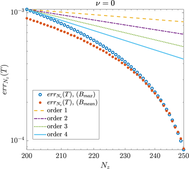
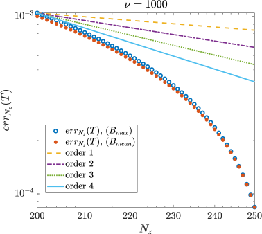
Figure 1: Two dimensional Sod shock tube test with control. Norm of the error for $\nu=0$ (on the left), $\nu=1000$ (on the right).

4.1.2 Effectiveness of the control strategy

To assess the effectiveness of the control strategy, we compute the thermal energy at the boundaries for each value $z_{i}$, with $i=1,\ldots,N_{z}$, as

$$\mathcal{E}_{b}^{n}(z_{i})=\frac{1}{2NN_{b}}\sum_{\mathcal{C}_{j}\in\Omega_{b}}\sum_{m=1}^{N}\left|{\bf v}_{m}^{n}(z_{i})-U_{b}^{n}(z_{i})\right|^{2}\chi({\bf x}_{m}^{n}\in\mathcal{C}_{j}),$$ (4.4)

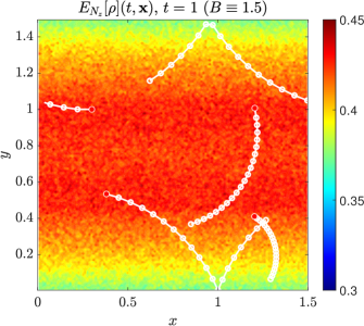
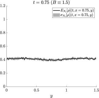
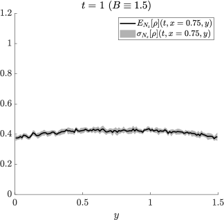
Figure 2: Two-dimensional Sod shock tube test with $B(t,{\bf x})=1.5$ and $\nu=0$. Top row: snapshots of the mean density at different time instants. Bottom row: slices of the mean density at $x=0.75$, with the corresponding standard deviation shown as a shaded area.

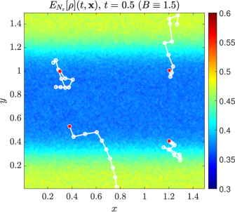
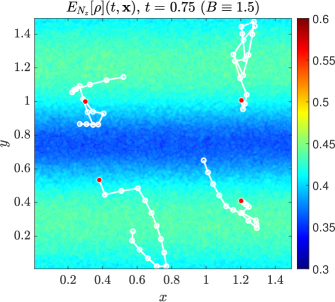
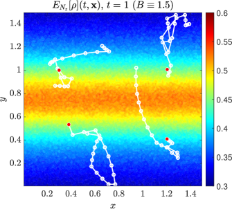
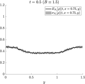
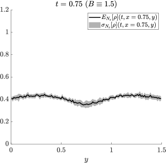
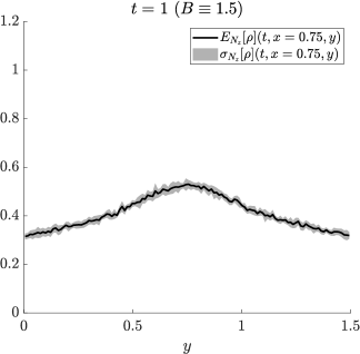
Figure 3: Two-dimensional Sod shock tube test with $B(t,{\bf x})=1.5$ and $\nu=10$. Top row: snapshots of the mean density at different time instants. Bottom row: slices of the mean density at $x=0.75$, with the corresponding standard deviation shown as a shaded area.

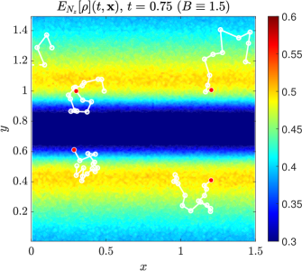
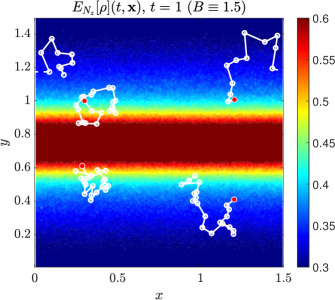
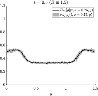
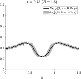
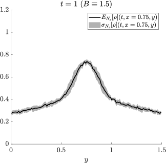
Figure 4: Two-dimensional Sod shock tube test with $B(t,{\bf x})=1.5$ and $\nu=1000$. Top row: snapshots of the mean density at different time instants. Bottom row: slices of the mean density at $x=0.75$, with the corresponding standard deviation shown as a shaded area.

where

$$\begin{split}U_{b}^{n}(z_{i})&=\frac{1}{NN_{b}\rho_{b}^{n}(z_{i})}\sum_{\mathcal{C}_{j}\in\Omega_{b}}\sum_{m=1}^{N}{\bf v}_{m}^{n}(z_{i})\chi({\bf x}_{m}^{n}\in\mathcal{C}_{j}),\\ \rho_{b}^{n}(z_{i})&=\frac{1}{NN_{b}}\sum_{\mathcal{C}_{j}\in\Omega_{b}}\sum_{m=1}^{N}\chi({\bf x}_{m}^{n}\in\mathcal{C}_{j}),\end{split}$$ (4.5)

and $N_{b}$ denotes the number of cells $\mathcal{C}_{j}\in\Omega_{b}$, with $\Omega_{b}=[0,0.234]\cup[1.476,1.5]$. This choice corresponds to a region near the $y$-boundaries with width equal to one cell size $\Delta_{y}$. We begin by considering the uncontrolled case, setting $B(t,{\bf x})=1.5$. Figures 2–3–4 illustrate the system dynamics under three different collisional regimes: $\nu=0$, $\nu=10$, and $\nu=1000$. In each figure, the first row displays snapshots of the mean density at times $t=0.5$, $t=0.75$, and $t=1$. Superimposed in white are the mean trajectories of four randomly selected particles up to time $t$, with their initial mean positions highlighted in red. The second row shows slices of the mean density function at $x=0.75$, taken at the same time instants, with the associated standard deviation represented as a shaded area. Initially, particles move toward the upper and lower boundaries of the domain, where they are reflected due to the imposed boundary conditions. As the collisional frequency $\nu$ increases, the diffusion of particles across the domain is progressively reduced. In the collisionless case ($\nu=0$), particles exhibit strong diffusive behavior. In contrast, in the highly collisional regime ($\nu=1000$), particles do not diffuse but instead oscillate around the center of the domain. The intermediate case ($\nu=10$) corresponds to a quasi-collisional regime, where both diffusion and collisional effects are simultaneously present. Figure 5 shows the mean thermal energy at the boundaries along with its standard deviation for $\nu=0$ (left), $\nu=10$ (center), and $\nu=1000$ (right). The thermal energy increases whenever particles collide with the boundaries. In the collisionless regime, the spatial diffusion of particles results in only minor variations in thermal energy. In contrast, in the quasi-collisional and fully collisional regimes, the thermal energy exhibits an oscillatory pattern, reflecting the behavior of the particle trajectories.

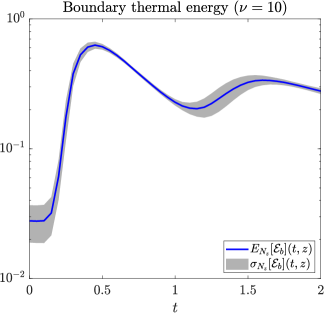
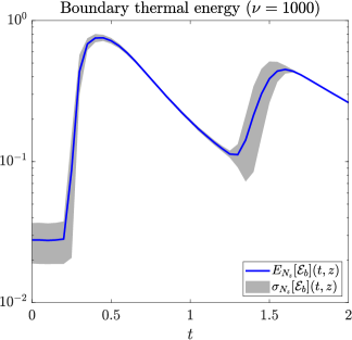
Figure 5: Two dimensional sod shock tube test without control. Thermal energy at the boundaries for $\nu=0$ (on the left), $\nu=10$ (in the centre) and $\nu=1000$ (on the right). The mean value is depicted in blue, while the standard deviation as a shaded area.

We now consider the case in which the magnetic field is computed as the solution of a control problem aimed at minimizing the percentage of mass reaching the lower and upper boundaries of the domain. To this end, we assume that the spatial region where the control is active is divided into $N_{c}$ horizontal cells, and we set $N_{c}=4$, unless otherwise specified. The maximum control magnitude is fixed at $M=50$, and the control parameters are chosen as follows: $\alpha_{\text{x}}=5$, $\beta_{\text{x}}=2$, $\alpha_{\text{v}}=15$, $\beta_{\text{v}}=12$, and $\gamma=2.5\times 10^{-3}$. The target position is set to $\hat{y}=0.75$, in order to drive the mass toward the center of the domain. Unless stated otherwise, the operator $\mathcal{P}(\cdot)$ is defined as in equation (2.14). The temperature at the boundaries is computed as

$$T_{b}^{n}(z_{i})=\rho_{b}^{n}(z_{i})\,\mathcal{E}_{b}^{n}(z_{i}),$$

for any $i=1,\ldots,N_{z}$, where $\rho_{b}^{n}(\cdot)$ and $\mathcal{E}_{b}^{n}(\cdot)$ are defined in equations (4.4)–(4.5). Figures 6–7–8 show the controlled dynamics for three different collisional regimes: $\nu=0$, $\nu=10$, and $\nu=1000$. In each figure, the first row displays snapshots of the mean density at times $t=0.5$, $t=0.75$, and $t=1$. The mean trajectories of four randomly selected particles are shown in white, with their initial positions highlighted in red. The second row shows slices of the mean density function at $x=0.75$, corresponding to the same time instants, with the associated standard deviation represented as a shaded area. Additionally, the values of the magnetic field $B(t,{\bf x})$ in each cell $C_{k}$ are displayed using a colorbar.

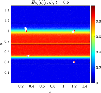
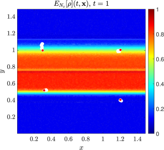
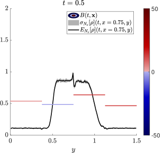
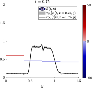
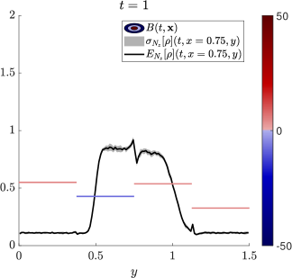
Figure 6: Two-dimensional Sod shock tube test with control and $\nu=0$. Top row: snapshots of the mean density at different time instants. Bottom row: slices of the mean density at $x=0.75$, with the corresponding standard deviation shown as a shaded area. The intensity of $B(t,{\bf x})$ in each cell $C_{k}$ is represented by the colorbar.

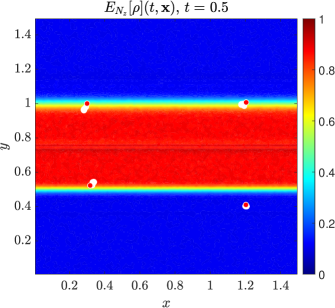
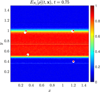
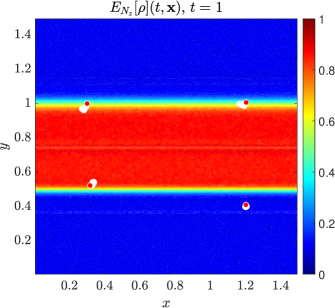
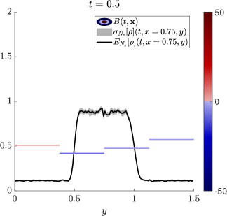
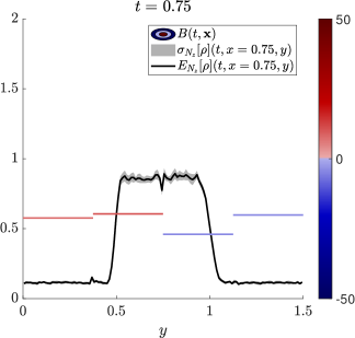
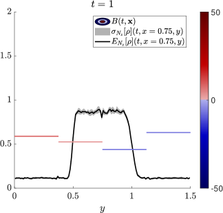
Figure 7: Two-dimensional Sod shock tube test with control and $\nu=10$. Top row: snapshots of the mean density at different time instants. Bottom row: slices of the mean density at $x=0.75$, with the corresponding standard deviation shown as a shaded area. The intensity of $B(t,{\bf x})$ in each cell $C_{k}$ is represented by the colorbar.

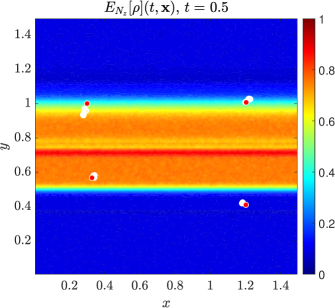
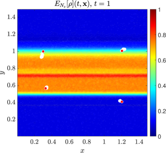
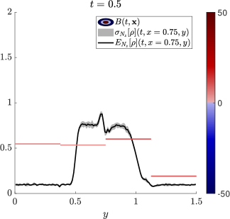
Figure 8: Two-dimensional Sod shock tube test with control and $\nu=1000$. Top row: snapshots of the mean density at different time instants. Bottom row: slices of the mean density at $x=0.75$, with the corresponding standard deviation shown as a shaded area. The intensity of $B(t,{\bf x})$ in each cell $C_{k}$ is represented by the colorbar.

Figure 9 shows, in the first row, the mean thermal energy at the boundaries, computed as in equation (4.4),for different values of $\nu$, along with the corresponding standard deviation depicted as a shaded area. In all cases considered, the thermal energy decreases over time as a result of the confinement of particles near the center of the domain, highlighting the effectiveness of the adopted control strategy. In the second row, the temporal evolution of the magnetic field is shown for the same values of $\nu$.

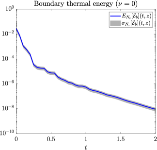
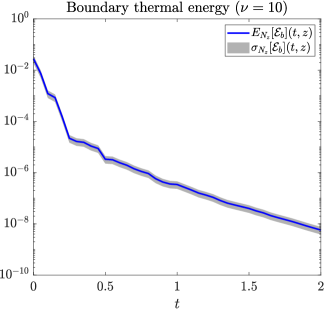
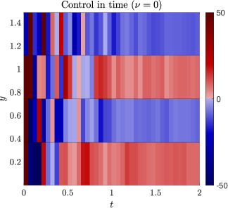
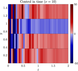
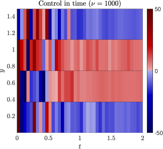
Figure 9: Two dimensional sod shock tube test with control. First row: mean thermal energy at the boundaries and the relative standard deviation depicted as a shaded area are shown. Second row: the value of the magnetic field is reported. On the left $\nu=0$, in the centre $\nu=10$, and on the right $\nu=1000$.

In Figure 10, we compare the thermal energy at the boundaries obtained using two different functionals within the control strategy. In particular, we consider the cases where $\mathcal{P}[\cdot]$ is defined as in equations (2.13) and (2.14), and denote the corresponding controls by $B_{\text{mean}}$ and $B_{\text{max}}$, respectively. For both cases, we plot the mean thermal energy at the boundaries along with the corresponding standard deviation, represented as a shaded area, under the same three collisional regimes previously considered. In all scenarios, the control strategy based on minimizing the worst-case behavior ($B_{\text{max}}$) proves to be slightly more effective than the one based on the average behavior ($B_{\text{mean}}$) in achieving the desired confinement.

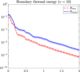
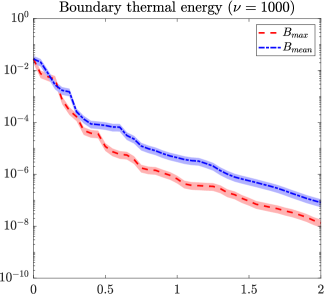
Figure 10: Two dimensional sod shock tube test with control. Mean thermal energy and relative standard deviation at the boundaries using $\mathcal{P}(\cdot)$ as defined in (2.14) (referred to as $B_{max}$) and (2.13) (referred to as $B_{mean}$). On the left $\nu=0$, in the centre $\nu=10$, and on the right $\nu=1000$.

We conclude by testing the effectiveness of the proposed control strategy under more challenging conditions, by increasing both the initial temperature of the plasma and the number of horizontal cells $N_{c}$ over which the control is active. For this test, we consider a deterministic setting by fixing $z=0$, and we assume the system operates in the fully collisional regime. Starting from the initial temperature $T_{0}$ defined in equation (4.2) (as used in the previous tests), we introduce three additional temperature profiles defined as follows:

$$\begin{split}\tilde{T}_{0}({\bf x})&=\chi(y\in[0,0.5)\cup(1,1.5))+10\,\chi(y\in[0.5,1]),\\ \bar{T}_{0}({\bf x})&=5\,\chi(y\in[0,0.5)\cup(1,1.5))+50\,\chi(y\in[0.5,1]),\\ \hat{T}_{0}({\bf x})&=10\,\chi(y\in[0,0.5)\cup(1,1.5))+100\,\chi(y\in[0.5,1]).\end{split}$$ (4.6)

The first row of Figure 11 shows, on the left, the evolution of thermal energy at the boundaries over time as the initial temperature increases, and on the right, the effect of varying the number of horizontal control cells $N_{c}$, for a fixed initial temperature $T_{0}({\bf x})=\hat{T}_{0}$. The second row reports the evolution in time of the control field for different values of $N_{c}$, again using $\hat{T}_{0}$ as the initial temperature. The results confirm that the effectiveness of the control strategy is inversely proportional to the initial plasma temperature, as expected. Moreover, the plot on the right suggests that increasing the number of horizontal cells does not lead to significant improvements in thermal energy reduction.

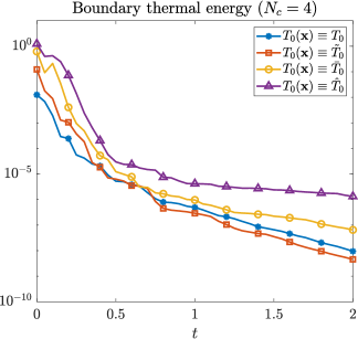
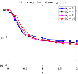
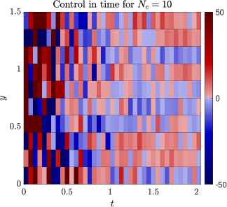
Figure 11: Two dimensional sod shock tube test with control. First row: thermal energy at the boundaries for different values of the initial temperature $T_{0}$ (left), thermal energy at the boundaries for different values of the number of cells $N_{c}$ (right). Second row: the value of the control in time as $N_{c}$ varies.

4.2 Kelvin-Helmholtz instability

In this section, we examine a variant of the Kelvin–Helmholtz instability in the context of charged particles; see [19, 47, 9]. We conduct an analysis similar to that of the previous section, comparing the controlled and uncontrolled scenarios in the presence of both uncertainty and collisions. Periodic boundary conditions are imposed in the $x$-direction, and reflective boundary conditions are imposed in the $y$-direction. The computational domain is defined as $x\in[0,40]$, $y\in[-5,5]$, and the initial density is given by

$$\rho_{0}({\bf x})=\frac{1.5}{2\pi}\,\text{sech}\left(\frac{y}{0.9}\right)\left(1+\epsilon_{0}\cos(3k_{0}x+\epsilon_{1}\sin(k_{0}x))\right),$$ (4.7)

with parameters $k_{0}=0.15$, $\epsilon_{0}=0.1$, and $\epsilon_{1}=0.001$. The initial distribution function is defined as

$$f_{0}({\bf x},{\bf v})=f_{0}^{+}({\bf x},{\bf v})\chi(y\geq 0)+f_{0}^{-}({\bf x},{\bf v})\chi(y<0),$$ (4.8)

where

$$f_{0}^{\pm}({\bf x},{\bf v})=\frac{\rho_{0}({\bf x})}{2\pi T_{0}({\bf x},z)}\exp\left(-\frac{(v_{x}\pm u_{x})^{2}+v_{y}^{2}}{2T_{0}({\bf x},z)}\right),$$ (4.9)

and $u_{x}=1$ is the mean velocity in the $x$-direction. The initial temperature includes uncertainty and is defined by

$$T_{0}({\bf x},z)=0.15+0.25z,$$ (4.10)

where $z\sim p(z)$ follows a uniform distribution over $[0,1]$.

Figure 12 displays the estimated initial mean distribution and thermal energy, reconstructed over a grid of size $m_{x}\times m_{y}$, with $m_{x}=m_{y}=128$. Simulations are performed using $N=10^{7}$ particles, up to final time $T=250$, with time step $h=0.5$. In the uncontrolled case, we set $B=1.5$, whereas in the controlled scenario, the control acts on $N_{c}=4$ horizontal cells. The mean density and thermal energy at the boundaries are computed as in equation (4.4), with the boundary region defined as $\Omega_{b}=[-5,-4.8]\cup[4.8,5]$.

4.2.1 Uncontrolled case

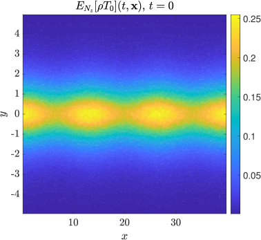
Figure 12: Kelvin-Helmholtz instability. Initial mean density and thermal energy.

Figure 13 shows the density field at times $t=50$, $t=75$, and $t=200$ for the uncontrolled case with $B=1.2$, across the three collisional regimes. In the fully collisional regime ($\nu=1000$), the instability develops rapidly, whereas in the collisionless regime ($\nu=0$) it emerges more gradually over time. An intermediate behavior is observed for the quasi-collisional case with $\nu=10$.

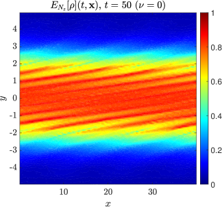
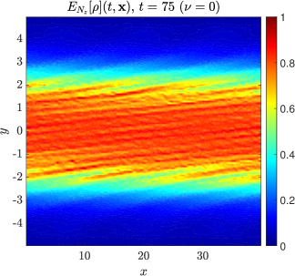
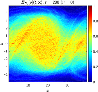
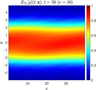
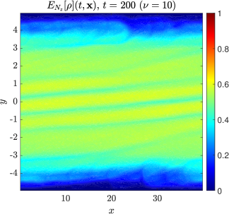
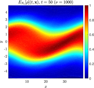
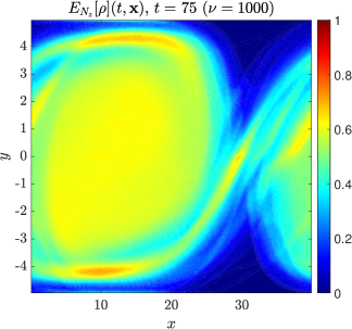
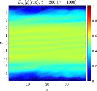
Figure 13: Kelvin-Helmholtz instability with $B(t,{\bf x})=1.2$. Mean density at $t=50$, $t=75$ and $t=200$. First row: $\nu=0$. Second row: $\nu=10$. Third row: $\nu=1000$.

In Figure 14 the thermal energy at the boundary in time for $\nu=0$ (on the left), $\nu=10$ (in the centre), and $\nu=1000$ (on the right) is shown. Once that the instability arises, the boundary thermal energy starts to increase.

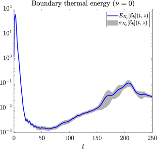
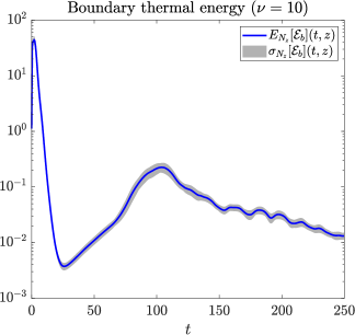
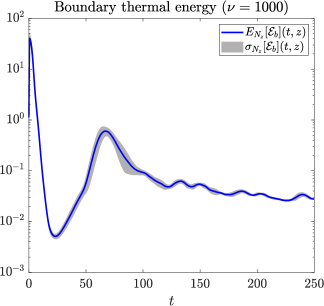
Figure 14: Kelvin-Helmholtz instability with $B(t,{\bf x})=1.2$. Thermal energy at the boundaries for $\nu=0$ (on the left), $\nu=10$ (in the centre) and $\nu=1000$ (on the right). The mean value is depicted in blue, while the standard deviation as a shaded area.

4.2.2 Feedback controlled case

The case of the robust control is shown in Figure 15, for the non collisional regime. We set $\alpha_{\textrm{x}}=5$,$\alpha_{\textrm{v}}=15$, $\beta_{\textrm{x}}=2$,$\beta_{\textrm{v}}=12$, and $\gamma=2.5\times 10^{-3}$, $M=100$, with target $\hat{y}=0$, to confine the mass at the center of the domain as for the previous case. In the first row, three snapshots of the dynamics taken at time $t=50$, $t=75$ and $t=200$ are depicted. In the second row the plot of the boundary thermal energy in time (on the left), and on control values in time in the four horizontal cells (on the right) can be observed. The figure demonstrates the effectiveness of the control strategy developed. Similar results are obtained in the quasi and fully collisional regimes for $\nu=10$, and $\nu=1000$, and are not shown for brevity.

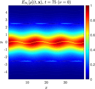
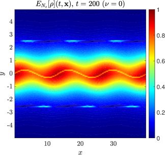
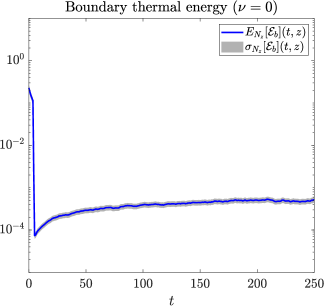
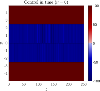
Figure 15: Kelvin-Helmholtz instability with control for $\nu=0$. First row: mean density at $t=50$, $t=75$ and $t=200$. Second row: thermal energy at the boundaries (on the left) and control (on the right). The mean thermal energy is depicted in blue, while the standard deviation as a shaded area.

5 Conclusions

In this work, we have proposed a new control strategy for the collisional Vlasov–Poisson–BGK system under uncertainty. The central idea is to develop an efficient instantaneous feedback control framework that steers the plasma toward a desired configuration through the application of an external magnetic field, which is constructed to be independent of the underlying randomness in the system.

To address the resulting optimization problem, we employed a semi-implicit Particle-In-Cell discretization for the Vlasov–Poisson system, combined with Monte Carlo sampling for the BGK collision process and a stochastic Gauss–Legendre quadrature method to represent uncertainty.

The control problem is formulated over a single time step, leading to an instantaneous feedback law derived via a simplified time integrator. The corresponding optimality system is solved through an augmented Lagrangian approach, ensuring enforcement of control constraints. The resulting feedback control is then integrated into the semi-implicit dynamics by considering the continuous-time limit as the time step vanishes.

Numerical experiments validate the effectiveness of the proposed control strategy across various collisional regimes, demonstrating its ability to confine the plasma and prevent boundary interactions. As directions for future work, we plan to explore alternative uncertainty quantification strategies, including multi-fidelity control variates, which aim to reduce computational cost by coupling low- and high-fidelity models. We also intend to tackle the additional complexity arising from the full Maxwell–Vlasov–BGK system, and to investigate the incorporation of more realistic collision operators, such as the Landau operator, within the proposed control framework.

Appendix A Comparison of different robust control strategies

In this Appendix, we first extend the control strategy introduced in [2] to the setting with uncertainty, and then compare it with the approach proposed in this work. Unlike the continuous control problem formulated in equation (2.9), where the control is computed for each particle and subsequently interpolated to obtain an average magnetic field, the strategy described in [2] directly computes a piecewise constant control (or magnetic field) within each fictitious cell $C_{k}$.

We briefly recall here the derivation of the instantaneous control strategy introduced in [2], extending it to account for uncertainty while, for simplicity, we assume a collisionless setting. We first formulate the problem at the continuous level and over a finite time horizon $[0,t_{f}]$ as follows

$$\min_{B\in\mathcal{B}_{adm}}\sum_{k=1}^{N_{c}}\mathcal{J}_{k}(B_{k}^{ext};f_{k},f^{0}_{k}),\qquad\textrm{s.t.}\leavevmode\nobreak\ \eqref{eq:Vlasov}-\eqref{eq:Poisson},$$ (A.1)

where $f_{k}=f_{k}(t,{\bf x},{\bf v},{\bf z})$ corresponds to the normalized particle density restricted to a single cell $C_{k}$

$$f_{k}(t,{\bf x},{\bf v},{\bf z})=\frac{f(t,{\bf x},{\bf v},{\bf z})}{\rho_{k}(t)},\qquad\rho_{k}(t)=\int_{\Omega_{k}}f(t,{\bf x},{\bf v},{\bf z})\,d{\bf x},d{\bf v},$$

with $\rho_{k}(t)>0$ the total cell density and with $B=(B_{1},\ldots,B_{N_{c}})$ now representing the vector of $z$ components of ${\bf B}(t,{\bf x})$ within each cell $C_{k}$, $\mathcal{B}_{adm}$ the set of admissible controls such that $\mathcal{B}_{adm}=\{B_{k}^{ext}|B_{k}^{ext}\in[-M,M],M>0,\,k=1,\ldots,N_{c}\}$, and where, for each $k=1,\ldots,N_{c}$, the cost functional is defined as follows

$$\begin{split}\mathcal{J}_{k}(B_{k};f_{k},f_{k}^{0})=&\int_{0}^{t_{f}}\left(\mathcal{P}\left[\mathcal{D}(f_{k})(t,{\bf z})\right]+\right.\\ &+\left.\frac{\gamma}{2}\mathcal{P}\left[\int_{\Omega_{k}}|B_{k}(t)|^{2}f_{k}(t,{\bf x},{\bf v},{\bf z})d{\bf x}d{\bf v}\right]\right)\,dt,\end{split}$$ (A.2)

where $\gamma>0$ is a penalization term, $\mathcal{P}[\cdot]$ is a suitable statistical operator taking into account the presence of the uncertainties, $\mathcal{D}(\cdot)$ aims at enforcing a specific configuration in the distribution function, and $\Omega_{k}=C_{k}\times\Omega_{v}$, being $\Omega_{v}$ the velocity domain. We consider a short time horizon of length $h>0$ and formulate a time discretize optimal control problem through the functional $\mathcal{J}_{k}$ restricted to the interval $[t,t+h]$, as follows

$$\min_{B_{k}\in\mathcal{B}_{adm}}\mathcal{J}^{N,h}_{k}(B_{k};f_{k}^{N},f_{k}^{N,0}),$$ (A.3)

subject to a semi-implicit in time discretized Vlasov dynamics, fully explicit for the velocity terms

$$\begin{split}&x_{m}^{n+1}({\bf z})=x_{m}^{n}({\bf z})+hv_{x_{m}}^{n+1}({\bf z}),\\ &y_{m}^{n+1}({\bf z},\xi)=y_{m}^{n}({\bf z})+hv_{y_{m}}^{n+1}({\bf z}),\\ &v_{x_{m}}^{n+1}({\bf z})=v_{x_{m}}^{n}({\bf z})+hv_{y_{m}}^{n}({\bf z})B_{m}^{n+1}+hE_{x_{m}}^{n}({\bf z}),\\ &v_{y_{m}}^{n+1}({\bf z})=v_{y_{m}}^{n}({\bf z})-hv_{x_{m}}^{n}({\bf z})B_{m}^{n+1}+hE_{y_{m}}^{n}({\bf z}).\end{split}$$ (A.4)

Using the rectangle rule for approximating the integral in time, and under the assumption that the magnetic field is independent of ${\bf z}$, the functional in (A.3) reads as follows

$$\mathcal{J}_{k}^{N,h}(B_{k};f_{k}^{N},f_{k}^{N,0})=h\left(\mathcal{P}[\mathcal{D}(f_{k}^{N})(t^{n+1},{\bf z})]+\frac{\gamma}{2}|B_{k}|^{2}\right).$$ (A.5)

Here we assume

$$\mathcal{D}(f_{k}^{N})(t,{\bf z})=\sum_{\ell\in{\{\textrm{x},\textrm{v}\}}}\mathcal{D}_{k}(f_{k}^{N},\phi_{\ell})(t^{n+1},{\bf z})$$ (A.6)

with $\mathcal{D}_{k}(f_{k}^{N},\phi_{\ell})(\cdot,{\bf z})$ as in (2.11), where we replace the full domain $\Omega$ with $\Omega_{k}$, for any $k=1,\ldots,N_{c}$. Thus, by setting $\phi_{\textrm{x}}=y^{n+1}$, $\phi_{\textrm{v}}=v_{y}^{n+1}$, $\hat{\phi}_{\textrm{x},k}=\hat{y}_{k}$ and $\hat{\phi}_{\textrm{v},k}=\hat{v}_{y_{k}}$, target states, and by direct computation over the empirical densities, we can rewrite the functional in (A.5) as

$$\begin{split}&\mathcal{J}_{k}^{N,h}(B_{k})=\mathcal{P}\left[\frac{h\alpha_{\emph{v}}}{2}|\bar{v}_{y,k}^{n+1}({\bf z})-\hat{v}_{y_{k}}|^{2}+\frac{h\beta_{\emph{v}}}{2N_{k}}\sum_{i\in C_{k}}|v_{y_{i}}^{n+1}({\bf z})-\bar{v}_{y,k}^{n}({\bf z})|^{2}+\right.\\ &\left.+\frac{h\alpha_{\emph{x}}}{2}|\bar{y}_{k}^{n+1}({\bf z})-\hat{y}_{k}|^{2}+\frac{h\beta_{\emph{x}}}{2N_{k}}\sum_{i\in C_{k}}|y_{i}^{n+1}({\bf z})-\bar{y}_{k}^{n}({\bf z})|^{2}+\frac{h\gamma}{2}|B^{n+1}_{k}|^{2}\right],\end{split}$$ (A.7)

with

$$\begin{split}\bar{y}_{k}({\bf z})=\frac{1}{N_{k}}\sum_{j\in C_{k}}y_{j}({\bf z}),\qquad\bar{v}_{y,k}({\bf z})=\frac{1}{N_{k}}\sum_{j\in C_{k}}v_{y_{j}}({\bf z}),\end{split}$$ (A.8)

denoting the mean position and velocity over cell $C_{k}$, $k=1,\ldots,N_{c}$. We extend now the result proved in [2] in the case of uncertainty.

Proposition 2.

Assume the parameters to scale as

$$\alpha_{\emph{x}}\rightarrow\frac{\alpha_{\emph{x}}}{h},\qquad\beta_{\emph{x}}\rightarrow\frac{\beta_{\emph{x}}}{h},\qquad\gamma\rightarrow\gamma h,$$ (A.9)

then the feedback control at cell $C_{k}$ associated to (A.7) reads as follows

$$B_{k}=\mathbb{P}_{[-M,M]}\left(\frac{\mathcal{P}[\mathcal{R}^{N,n}_{\emph{v},k}({\bf z})+\mathcal{R}^{N,n}_{\emph{x},k}({\bf z})]}{\gamma+\mathcal{P}[\mathcal{S}^{N,n}_{\emph{v},k}({\bf z})+\mathcal{S}^{N,n}_{\emph{x},k}({\bf z})]}\right),$$ (A.10)

where $\gamma>0$,

$$\begin{split}&\mathcal{R}^{N,n}_{\emph{v},k}({\bf z})=\alpha_{\emph{v}}(\bar{v}_{y,k}^{n}({\bf z})+h\bar{E}_{y,k}^{n}({\bf z})-\hat{v}_{y_{k}})\bar{v}^{n}_{x,k}({\bf z})+\\ &\qquad\qquad\qquad+\frac{\beta_{\emph{v}}}{N_{k}}\sum_{i=1}^{N_{k}}\left[(v_{y_{i}}^{n}({\bf z})+hE_{y_{i}}^{n}({\bf z})-\bar{v}_{y,k}^{n}({\bf z}))v_{x_{i}}^{n}({\bf z})\right],\\ &\mathcal{R}^{N,n}_{\emph{x},k}({\bf z})=\alpha_{\emph{x}}(\bar{y}_{k}^{n}({\bf z})+h(\bar{v}_{y,k}^{n}({\bf z})+h\bar{E}_{y,k}^{n}({\bf z}))-\hat{y}_{k})\bar{v}^{n}_{x,k}({\bf z})+\\ &\qquad\qquad\qquad+\frac{\beta_{\emph{x}}}{N_{k}}\sum_{i=1}^{N_{k}}\left[(y_{i}^{n}({\bf z})+h(v_{y_{i}}^{n}({\bf z})+hE_{y_{i}}^{n}({\bf z}))-\bar{y}_{k}^{n}({\bf z}))v_{x_{i}}^{n}({\bf z})\right],\\ &\mathcal{S}^{N,n}_{\emph{v},k}({\bf z})=h\left(\alpha_{\emph{v}}(\bar{v}_{x,k}^{n}({\bf z}))^{2}+\frac{\beta_{\emph{v}}}{N_{k}}\sum_{i=1}^{N_{k}}(v_{x_{i}}^{n}({\bf z}))^{2}\right),\\ &\mathcal{S}^{N,n}_{\emph{x},k}({\bf z})=h^{2}\left(\alpha_{\emph{x}}(\bar{v}_{x,k}^{n}({\bf z}))^{2}+\frac{\beta_{\emph{x}}}{N_{k}}\sum_{i=1}^{N_{k}}(v_{x_{i}}^{n}({\bf z}))^{2}\right),\end{split}$$ (A.11)

and with $\mathbb{P}_{[-M,M]}(\cdot)$ denoting the projection over the interval $[-M,M]$. In the limit $h\to 0$ the control at the continuous level reads,

$$B_{k}(t)=\mathbb{P}_{[-M,M]}\left(\frac{1}{\gamma}\left(\mathcal{P}\left[\mathcal{R}^{N}_{\emph{v},k}(t,{\bf z})+\mathcal{R}^{N}_{\emph{x},k}(t,{\bf z})\right]\right)\right),$$ (A.12)

with

$$\begin{split}&\mathcal{R}^{n}_{\emph{v},k}(t,{\bf z})=\alpha_{\emph{v}}(\bar{v}_{y,k}(t,{\bf z})-\hat{v}_{y_{k}})\bar{v}_{x,k}(t,{\bf z})+\frac{\beta_{\emph{v}}}{N_{k}}\sum_{i\in C_{k}}(v_{y_{i}}(t,{\bf z})-\bar{v}_{y,k}(t,{\bf z}))v_{x_{i}}(t,{\bf z}),\\ &\mathcal{R}^{n}_{\emph{x},k}(t,{\bf z})=\alpha_{\emph{x}}(\bar{y}_{k}(t,{\bf z})-\hat{y}_{k})\bar{v}_{x,k}(t,{\bf z})+\frac{\beta_{\emph{x}}}{N_{k}}\sum_{i\in C_{k}}(y_{i}(t,{\bf z})-\bar{y}_{k}(t,{\bf z}))v_{x_{i}}(t,{\bf z}).\end{split}$$

We now focus on the two-dimensional Sod test discussed in Section 4.1, using the same numerical setting. We consider a collisionless regime and introduce uncertainty in the system by sampling $N_{z}=10$ Gauss–Legendre nodes. We compare the instantaneous controls defined in equations (3.17) and (A.12), using the parameters $\alpha_{\text{x}}=5$, $\beta_{\text{x}}=2$, $\alpha_{\text{v}}=15$, $\beta_{\text{v}}=12$, $\gamma=2.5\times 10^{-3}$, and $M=50$, with $\mathcal{P}(\cdot)$ defined as in equation (2.14). The simulation is carried out up to final time $t_{f}=2$, with a time step $h=0.05$. Figure 16 summarizes the results. On the left, we report the mean thermal energy at the boundaries along with the corresponding standard deviation. In the center and on the right, we show the magnetic field values. In the first row, the initial temperature is defined as in equation (4.2), while in the second row it corresponds to the high-temperature configuration given in equation (4.6) (last equation). In both cases, the new control strategy proposed in this work proves to be more effective in reducing thermal energy compared to the approach introduced in [2], with the improvement being particularly significant in high-temperature scenarios.

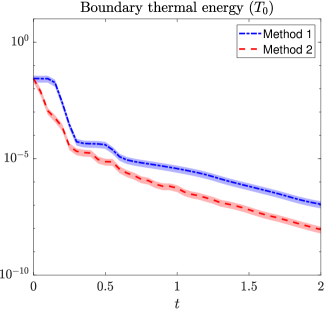
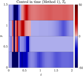
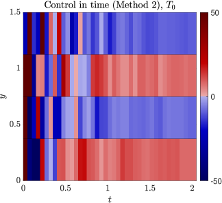
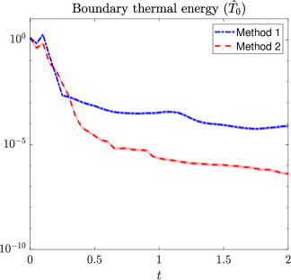
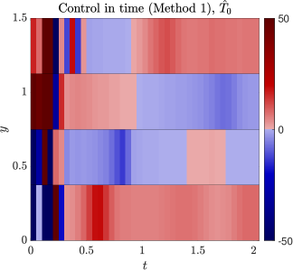
Figure 16: Two dimensional Sod shock tube test with control. Comparison between the two control strategies, (A.10) (Method 1) and (3.17) (Method 2) in terms of thermal energy at the boundaries (on the left) and of magnetic field value (in the center and on the right). The different lines depict the mean thermal energy at the boundaries, while the shaded areas represent the standard deviation.

References

- [1] G. Albi, Y.-P. Choi, M. Fornasier, and D. Kalise. Mean field control hierarchy. Applied Mathematics & Optimization, 76:93–135, 2017.
- [2] G. Albi, G. Dimarco, F. Ferrarese, and L. Pareschi. Instantaneous control strategies for magnetically confined fusion plasma. Journal of Computational Physics, page 113804, 2025.
- [3] J. Bartsch, P. Knopf, S. Scheurer, and J. Weber. Controlling a Vlasov–Poisson plasma by a Particle-In-Cell method based on a Monte Carlo framework. SIAM Journal on Control and Optimization, 62(4):1977–2011, 2024.
- [4] R. Belaouar, N. Crouseilles, P. Degond, and E. Sonnendrücker. An asymptotically stable semi-Lagrangian scheme in the quasi-neutral limit. Journal of Scientific Computing, 41:341–365, 2009.
- [5] J. Blum. Numerical simulation and optimal control in plasma physics. New York, NY; John Wiley and Sons Inc., 1989.
- [6] R. Caflisch, C. Wang, G. Dimarco, B. Cohen, and A. Dimits. A hybrid method for accelerated simulation of Coulomb collisions in a plasma. SIAM Multiscale Modeling & Simulation, 7(2):865–887, 2008.
- [7] R. E. Caflisch. Monte Carlo and Quasi Monte Carlo methods. Acta Numerica, 7:1–49, 1998.
- [8] S. Caprino, G. Cavallaro, and C. Marchioro. Time evolution of a Vlasov-Poisson plasma with magnetic confinement. Kinetic & Related Models, 5(4), 2012.
- [9] E. Chacon-Golcher, S. A. Hirstoaga, and M. Lutz. Optimization of Particle-In-Cell simulations for Vlasov–Poisson system with strong magnetic field. ESAIM: Proc., 53:177–190, 2016.
- [10] G. Chen and L. Chacón. An implicit, conservative and asymptotic-preserving electrostatic Particle-In-Cell algorithm for arbitrarily magnetized plasmas in uniform magnetic fields. Journal of Computational Physics, 487:Paper No. 112160, 16, 2023.
- [11] C.-Z. Cheng and G. Knorr. The integration of the Vlasov equation in configuration space. Journal of Computational Physics, 22(3):330–351, 1976.
- [12] Y. Cheng, I. M. Gamba, F. Li, and P. J. Morrison. Discontinuous Galerkin methods for the Vlasov–Maxwell equations. SIAM Journal on Numerical Analysis, 52(2):1017–1049, 2014.
- [13] S. W. Chung, S. D. Bond, E. C. Cyr, and J. B. Freund. Regular sensitivity computation avoiding chaotic effects in Particle-In-Cell plasma methods. Journal of Computational Physics, 400:108969, 32, 2020.
- [14] J. Coughlin and J. Hu. Efficient dynamical low-rank approximation for the Vlasov-Ampère-Fokker-Planck system. Journal of Computational Physics, 470:Paper No. 111590, 20, 2022.
- [15] J. Coughlin and J. Hu. Efficient dynamical low-rank approximation for the Vlasov-Ampere-Fokker-Planck system. Journal of Computational Physics, 470:111590, 2022.
- [16] A. Crestetto, N. Crouseilles, and M. Lemou. Kinetic/fluid micro-macro numerical schemes for Vlasov-Poisson-BGK equation using particles. Kinetic and Related Models, 5(4):787–816, 2012.
- [17] N. Crouseilles, G. Dimarco, and M.-H. Vignal. Multiscale schemes for the BGK–Vlasov–Poisson system in the quasi-neutral and fluid limits. stability analysis and first order schemes. SIAM Multiscale Modeling & Simulation, 14(1):65–95, 2016.
- [18] N. Crouseilles and F. Filbet. Numerical approximation of collisional plasmas by high order methods. Journal of Computational Physics, 201(2):546–572, 2004.
- [19] N. Crouseilles, M. Mehrenberger, and E. Sonnendrücker. Conservative semi-Lagrangian schemes for Vlasov equations. Journal of Computational Physics, 229(6):1927–1953, 2010.
- [20] P. Degond. Asymptotic-preserving schemes for fluid models of plasmas. In Numerical models for fusion, volume 39/40 of Panorama & Synthèses, pages 1–90. Soc. Math. France, Paris, 2013.
- [21] P. Degond and F. Deluzet. Asymptotic-preserving methods and multiscale models for plasma physics. Journal of Computational Physics, 336:429–457, 2017.
- [22] P. Degond, F. Deluzet, L. Navoret, A.-B. Sun, and M.-H. Vignal. Asymptotic-preserving Particle-In-Cell method for the Vlasov-Poisson system near quasineutrality. Journal of Computational Physics, 229(16):5630–5652, 2010.
- [23] G. Dimarco, R. Caflisch, and L. Pareschi. Direct simulation Monte Carlo schemes for Coulomb interactions in plasmas. Communications in Applied and Industrial Mathematics, 1(1):72–91, 2010.
- [24] G. Dimarco, Q. Li, L. Pareschi, and B. Yan. Numerical methods for plasma physics in collisional regimes. Journal of Plasma Physics, 81(1), 2015.
- [25] G. Dimarco, L. Mieussens, and V. Rispoli. An asymptotic preserving automatic domain decomposition method for the Vlasov-Poisson-BGK system with applications to plasmas. Journal of Computational Physics, 274:122–139, 2014.
- [26] G. Dimarco and L. Pareschi. Multi-scale control variate methods for uncertainty quantification in kinetic equations. Journal of Computational Physics, 388:63–89, 2019.
- [27] G. Dimarco and L. Pareschi. Multiscale variance reduction methods based on multiple control variates for kinetic equations with uncertainties. SIAM Multiscale Modeling & Simulation, 18(1):351–382, 2020.
- [28] G. Dimarco, L. Pareschi, and M. Zanella. Micro-macro stochastic Galerkin methods for nonlinear Fokker-Planck equations with random inputs. SIAM Multiscale Modeling & Simulation, 22(1):527–560, 2024.
- [29] L. Einkemmer, Q. Li, C. Mouhot, and Y. Yue. Control of instability in a Vlasov-Poisson system through an external electric field. Journal of Computational Physics, 530:113904, 2025.
- [30] L. Einkemmer, Q. Li, L. Wang, and Y. Yunan. Suppressing instability in a Vlasov–Poisson system by an external electric field through constrained optimization. Journal of Computational Physics, 498:112662, 2024.
- [31] F. Filbet and L. M. Rodrigues. Asymptotically stable Particle-In-Cell methods for the Vlasov–Poisson system with a strong external magnetic field. SIAM Journal on Numerical Analysis, 54(2):1120–1146, 2016.
- [32] F. Filbet and L. M. Rodrigues. Asymptotically preserving Particle-In-Cell methods for inhomogeneous strongly magnetized plasmas. SIAM Journal on Numerical Analysis, 55(5):2416–2443, 2017.
- [33] F. Filbet and E. Sonnendrücker. Numerical methods for the Vlasov equation. In Numerical Mathematics and Advanced Applications: Proceedings of ENUMATH 2001 the 4th European Conference on Numerical Mathematics and Advanced Applications Ischia, July 2001, pages 459–468. Springer, 2003.
- [34] A. Gu, Y. He, and Y. Sun. Hamiltonian Particle-In-Cell methods for Vlasov–Poisson equations. Journal of Computational Physics, 467:111472, 2022.
- [35] J. Hu, S. Jin, and R. Shu. A stochastic Galerkin method for the Fokker-Planck-Landau equation with random uncertainties. In Theory, numerics and Applications of Hyperbolic Problems. IIumerics and applications of hyperbolic problems. II, volume 237 of Springer Proc. Math. Stat., pages 1–19. Springer, Cham, 2018.
- [36] S. Jin and Y. Zhu. Hypocoercivity and uniform regularity for the Vlasov-Poisson-Fokker-Planck system with uncertainty and multiple scales. SIAM Journal on Mathematical Analysis, 50(2):1790–1816, 2018.
- [37] P. Knopf and J. Weber. Optimal control of a Vlasov–Poisson plasma by fixed magnetic field coils. Applied Mathematics & Optimization, 81:961–988, 2020.
- [38] Y. Lin and S. Jin. Error estimates of a bi-fidelity method for a multi-phase Navier-Stokes-Vlasov-Fokker-Planck system with random inputs. Kinetic and Related Models, 17(5):807–837, 2024.
- [39] A. Medaglia, L. Pareschi, and M. Zanella. Stochastic Galerkin particle methods for kinetic equations of plasmas with uncertainties. Journal of Computational Physics, 479:112011, 2023.
- [40] A. Medaglia, L. Pareschi, and M. Zanella. Particle simulation methods for the Landau-Fokker-Planck equation with uncertain data. Journal of Computational Physics, 503:112845, 2024.
- [41] F. Nobile, R. Tempone, and C. G. Webster. A sparse grid stochastic collocation method for partial differential equations with random input data. SIAM J. Num. Anal., 46(5):2309–2345, 2008.
- [42] L. Pareschi and G. Russo. An introduction to Monte Carlo methods for the Boltzmann equation. In CEMRACS 1999 (Orsay), volume 10 of ESAIM Proc., pages 35–76. Soc. Math. Appl. Indust., Paris, 1999.
- [43] L. Pareschi and G. Russo. Time relaxed Monte Carlo methods for the Boltzmann equation. SIAM Journal on Scientific Computing, 23(4):1253–1273, 2001.
- [44] L. Pareschi and S. Trazzi. Numerical solution of the Boltzmann equation by time relaxed Monte Carlo (TRMC) methods. International journal for numerical methods in fluids, 48(9):947–983, 2005.
- [45] G. Russo and F. Filbet. Semilagrangian schemes applied to moving boundary problems for the BGK model of rarefied gas dynamics. Kinetic and related models, 2(1):231–250, 2009.
- [46] L. Saint-Raymond. The gyrokinetic approximation for the Vlasov–Poisson system. Mathematical Models and Methods in Applied Sciences, 10(09):1305–1332, 2000.
- [47] E. Sonnendrücker, J. Roche, P. Bertrand, and A. Ghizzo. The semi-lagrangian method for the numerical resolution of the Vlasov equation. Journal of computational physics, 149(2):201–220, 1999.
- [48] L. Spitzer, Jr. The stellarator concept. Physics of Fluids, 1:253–264, 1958.
- [49] W. T. Taitano, D. A. Knoll, and L. Chacón. Charge-and-energy conserving moment-based accelerator for a multi-species Vlasov-Fokker-Planck-Ampère system, part II: collisional aspects. Journal of Computational Physics, 284:737–757, 2015.
- [50] W. T. Taitano, D. A. Knoll, L. Chacón, and G. Chen. Development of a consistent and stable fully implicit moment method for Vlasov-Ampère particle in cell (PIC) system. SIAM J. Sci. Comput., 35(5):S126–S149, 2013.
- [51] T. Xiao and M. Frank. A stochastic kinetic scheme for multi-scale plasma transport with uncertainty quantification. Journal of Computational Physics, 432:110–139, 2021.
- [52] D. Xiu and J. S. Hesthaven. High-order collocation methods for differential equations with random inputs. SIAM Journal on Scientific Computing, 27(3):1118–1139, 2005.
- [53] C. Yang and F. Filbet. Conservative and non-conservative methods based on hermite weighted essentially non-oscillatory reconstruction for Vlasov equations. Journal of Computational Physics, 279:18–36, 2014.
- [54] Y. Yudin, D. Coster, U. von Toussaint, and F. Jenko. Epistemic and aleatoric uncertainty quantification and surrogate modelling in high-performance multiscale plasma physics simulations. In Computational Science – ICCS 2023, volume 10476 of Lecture Notes in Computer Science, pages 572–586. Springer, 2023.
- [55] Y. Zhu and S. Jin. The Vlasov-Poisson-Fokker-Planck system with uncertainty and a one-dimensional asymptotic preserving method. SIAM Multiscale Modeling & Simulation, 15(4):1502–1529, 2017.