SPARS: Self-Play Adversarial Reinforcement Learning for Segmentation of Liver Tumours

Abstract

Accurate tumour segmentation is vital for various targeted diagnostic and therapeutic procedures for cancer, e.g., planning biopsies or tumour ablations. Manual delineation is extremely labour-intensive, requiring substantial expert time. Fully-supervised machine learning models aim to automate such localisation tasks, but require a large number of costly and often subjective 3D voxel-level labels for training. The high-variance and subjectivity in such labels impacts model generalisability, even when large datasets are available. Histopathology labels may offer more objective labels but the infeasibility of acquiring pixel-level annotations to develop tumour localisation methods based on histology remains challenging in-vivo. In this work, we propose a novel weakly-supervised semantic segmentation framework called SPARS (Self-Play Adversarial Reinforcement Learning for Segmentation), which utilises an object presence classifier, trained on a small number of image-level binary cancer presence labels, to localise cancerous regions on CT scans. Such binary labels of patient-level cancer presence can be sourced more feasibly from biopsies and histopathology reports, enabling a more objective cancer localisation on medical images. Evaluating with real patient data, we observed that SPARS yielded a mean dice score of $77.3\pm 9.4$, which outperformed other weakly-supervised methods by large margins. This performance was comparable with recent fully-supervised methods that require voxel-level annotations. Our results demonstrate the potential of using SPARS to reduce the need for extensive human-annotated labels to detect cancer in real-world healthcare settings.
Code: github.com/catalinatan/SPARS

1 Introduction

Tumour segmentation is crucial for diagnosing and treating liver cancer, particularly in its early stages [11, 2, 31, 7, 33]. For instance, identifying cancerous lesions from medical scans can enable clinicians to estimate the tumour diameters and volumes required for targeted radiation delivery in radiotherapies, where radiation dose varies with tumour size [31]. Currently, radiologists manually delineate tumour boundaries on each slice of 3D computed tomography (CT) and/ or magnetic resonance imaging (MRI) scans [11]. However, this manual delineation may be subjective, time-consuming and poorly reproducible [5, 9, 13]. The subjectivity leads to high inter- and intra-clinician variability in such tasks, which may be a result of the morphological diversity of tumour appearances on these scans as well as varying institute-specific training and expertise [5, 9]. These problems underscore the need for more reproducible and objective tumour localisation for cancer interventions [12, 18].

Automated segmentation methods aim to address the reproducibility of tumour localisation using fully-supervised learning, where a large number of labels that may be curated through consensus of multiple experts are used to train an automated model. However, this requires a large number of voxel-level expert-annotated labels that are very costly to obtain, especially if curated with a consensus from multiple experts [6, 11, 19, 27].

To mitigate the challenges that plague fully-supervised learning, weakly-supervised learning has been explored for a variety of tasks. Weak supervision allows the use of weak labels (during training or model development) to perform complex tasks at inference. Examples include training neural networks to perform pixel-level segmentation using only bounding boxes [16, 10], scribbles [24, 21] or image-level annotations [1, 17, 29, 25, 35] during training. In particular, image-level classification labels present great promise for weakly-supervised semantic segmentation (WSSS) due to the comparatively lower cost of their acquisition [19]. However, achieving comparable performance to fully-supervised learning, especially in complex clinical tasks such as tumour localisation, remains an open challenge.

In this work we propose a novel framework for WSSS, where we use a minimal number of image-level labels of cancer presence during model development to allow a voxel-level tumour segmentation at inference. The image-level cancer presence labels are objective histopathology labels which indicate whether each patient has clinically significant cancer or not. These image-level labels are used to train an object presence classifier which can classify ROI (region-of-interest) presence within an image. At inference, we use this classifier to generate logits (classification probability) for a section or window of the image, which serves as a likelihood of object presence within the window. For localisation of ROIs, we use self-play adversarial reinforcement learning (RL) where two agents compete to localise ROIs. Each agent moves a window across an image and is rewarded based on the classifier output for the window indicating object presence likelihood. Training to maximise the reward allows each agent to improve localisation towards areas where the likelihood of object presence is maximised. Tracking the classifier outputs for each window, we can generate a voxel-level probability map (described in Sec. 2.4), where a threshold can control which voxels are to be included as positive or negative for the final segmentation. This allows greater application-specific flexibility compared to other weakly-supervised methods, with fixed localisation termination conditions [29, 35, 25].

The contributions of our work are summarised:

1. we propose a self-play adversarial RL framework for WSSS to minimise manual segmentation costs;

2. we propose to supervise the adversarial RL framework using a classifier trained on image-level labels of object presence to quantify ROI presence likelihood which forms the rewards for RL-based WSSS;

3. our method allows greater application-specific flexibility compared to other WSSS methods by generating a pixel-level classification map (as opposed to patch-level [29, 25]) which can be thresholded to adjust which pixels to include as positive or negative

4. we evaluate our method using data from real liver cancer patients, to localise tumours on CT scans, and compare with recent state-of-the-art weakly- and fully-supervised algorithms demonstrating superior performance to weakly-supervised, and comparable performance to fully-supervised, approaches;

5. we make our algorithm openly available: github.com/catalinatan/SPARS

2 Methods

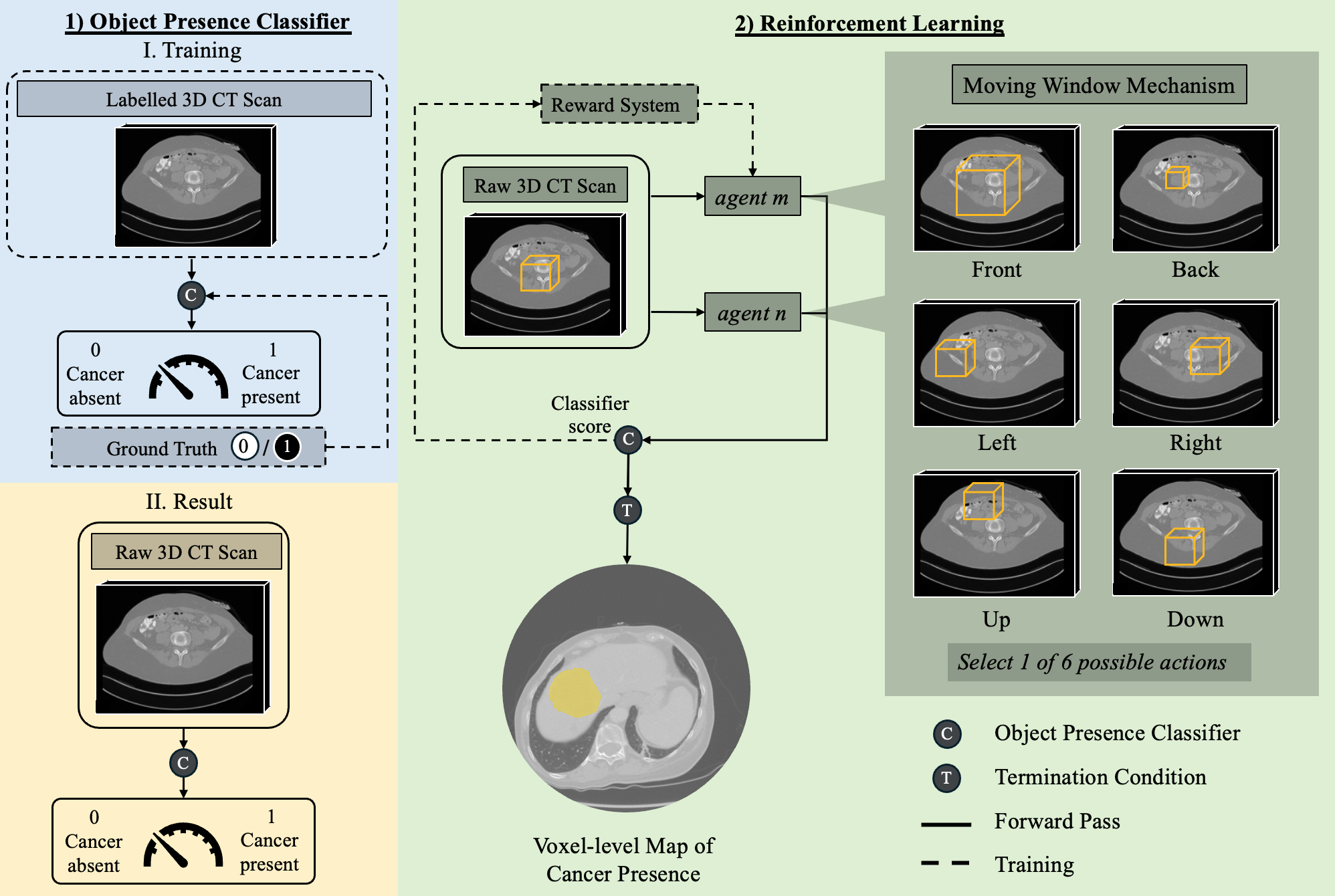
Figure 1: An overview of the proposed method, where two agents compete to localise ROIs guided by a classifier trained only using weak classification labels.

2.1 Object Presence Classifier

The object presence classifier $f(\cdot;w):\mathcal{X}\rightarrow[0,1]$, generates a score for a given image sample $x\in\mathcal{X}$ where $\mathcal{X}$ is the image domain and $w$ represents the neural network parameters. This is modelled as a mechanism to provide a linkage function between the two differing weak and full objectives, here, image-level and pixel-level classifications [25, 29, 4, 32, 28]. These network parameters are optimised using image-label pairs which indicate object presence in the sample, denoted as $\left\{x_{i},y_{i}\right\}_{i=1}^{N}$ where $y_{i}\in\mathcal{Y}$ with $\mathcal{Y}$ being the label domain $\{0,1\}$ and $N$ is the number of samples in the set. If the region of interest (ROI) is contained in $x_{i}$, its corresponding binary label is given by $y_{i}=1$. Conversely, $y_{i}=0$ if the ROI is not present.

The classifier is trained using the binary cross-entropy loss function:

$$l(y_{i},f(x_{i};w))=-\frac{1}{N}\sum^{N}_{i=1}(y_{i}\log(f(x_{i};w))+(1-y_{i})\log(1-f(x_{i};w))$$

where $f(x_{i};w)$ is the predicted label by the classifier and $y_{i}$ is the ground truth label for an image $x_{i}$.

The network parameters $w$ are optimised by minimising the expected loss function:

$$w^{\ast}=\arg\min_{w}~\mathbb{E}_{x_{i}\in\mathcal{X},y_{i}\in\mathcal{Y}}[l(y_{i},f(x_{i};w)]$$

where $w^{\ast}$ represents the optimal parameters.

2.2 Markov decision process environment

In RL, an agent (neural network) interacts with an environment by producing actions. In response to agent actions, the environment generates new states that are observed by the agent, and rewards that inform the agent of the impact of its actions. The rewards are used to train the agent to predict optimal actions given states. The agent-environment interactions are modelled as a Markov decision process that iterates sequentially, and is represented by a tuple $(\mathcal{S},\mathcal{A},p,r,\pi,\gamma)$, where $\mathcal{S}$ denotes the state space, $\mathcal{A}$ represents the action space, $p$ defines the state transition probability, $r$ is the reward, $\pi$ is the agent or policy, and $\gamma$ represents the discount factor for future rewards.

States: The observed states are cropped windows $x_{i}^{(a,b,c)}$, where $x_{i}$ is the entire image and $(a,b,c)$ denote the locations of a fixed-size crop in the height, width and depth dimensions respectively (a hyper-parameter investigated in Sec. 4.1.1). The state $s_{t}\in\mathcal{S}$ at time-step $t$ is therefore given by $s_{t}=\{x_{i}^{(a,b,c)}\}$, where $\mathcal{S}$ denotes the state space.

Actions: The actions can move the window $x_{i}^{(a,b,c)}$ in any direction. The action $a_{t}\in\mathcal{A}$ is given by $a_{t}=(\delta a,\delta b,\delta c)$. The actions are modelled discretely, only allowing a movement by a fixed distance in one of 6 directions, which means that $(\delta a,\delta b,\delta c)\in\{(\pm d,0,0),(0,\pm d,0),(0,0,\pm d)\}$, where only one of $\delta a$, $\delta b$, or $\delta c$ can be non-zero (i.e., $\pm d$), while the others must be zero.

State transitions: Given the current state $s_{t}=\{x_{i}^{(a,b,c)}\}$ and action $a_{t}=(\delta a,\delta b,\delta c)$, the next state $s_{t+1}=\{x_{i}^{(a+\delta a,~b+\delta b,~c+\delta c)}\}$. So the action moves the window to a new location. The probability of transitioning to the next state $s_{t+1}$, given current state $s_{t}$ and action $a_{t}$ is given by $p(\cdot):\mathcal{S}\times\mathcal{S}\times\mathcal{A}\rightarrow[0,1]$, which can be expressed as $p(s_{t+1}|s_{t},a_{t})$ for a particular time-step $t$.

Policy: The policy or agent $\pi(\cdot;\theta):\mathcal{S}\rightarrow\mathcal{A}$ predicts the action $a_{t}$, given the state $s_{t}$, where $\theta$ represents the parameters of the policy and $a_{t}=\pi(s_{t};\theta)$. Note that in this work we model the policy stochastically where $\pi(\cdot;\theta):\mathcal{S}\times\mathcal{A}\rightarrow[0,1]$, which gives the probability whereby $a_{t}\sim\pi(\cdot|s_{t})$, however, the notation of $a_{t}=\pi(s_{t};\theta)$ is adopted for simplicity.

2.3 Policy optimisation using self-play adversarial RL

The use of two competing agents to localise ROIs ensures that the impact of any errors in the object presence classifier are minimised since rewards for training are based on a comparison rather than exact object presence classifier outputs. Furthermore, using experience from two agents allows convergence with fewer time-steps compared to using only one set of experiences for training. Previous works have also shown the efficacy of using self-play in object localisation [29].

In our work we use self-play adversarial RL, where there are two versions of the policy, denoted as $\pi_{m}(\cdot;\theta_{m})$ and $\pi_{n}(\cdot;\theta_{n})$, where the only difference is the parameters. In further analyses subscripts $m$ and $n$ will denote outputs from polices $m$ and $n$ respectively. In this work, $\theta_{m}=\theta_{n}$. Since the policy is modelled stochastically, the actions selected by each may differ at any single time-step.

Rewards: A reward function $r(\cdot):\mathcal{S}\times\mathcal{A}\rightarrow\mathbb{R}$ predicts a reward $R_{t}\in\mathbb{R}$, given the state $s_{t}$ and action $a_{t}$. For policy $\pi_{m}$, the state, action, reward triplet is given by $(s_{m,t},a_{m,t},R_{m,t})$ and for policy $\pi_{n}$ by $(s_{n,t},a_{n,t},R_{n,t})$. The reward for $\pi_{m}$ is given by:

$$R_{m,t}=\begin{cases}+1&\text{if }f(s_{m,t};w^{*})\geq f(s_{n,t};w^{*})\\ -1&\text{otherwise}\end{cases}$$

This means that a positive reward is given for policy $\pi_{m}$ when the likelihood of object presence as measured by the trained object presence classifier for the window $s_{m,t}$, given by $f(s_{m,t};w^{*})$, is greater than the likelihood of object presence for the window $s_{n,t}$, given by $f(s_{n,t};w^{*})$.

The reward for $\pi_{n}$ is just the opposite of reward for $\pi_{m}$ and is given by $R_{n,t}=-R_{m,t}$.

Despite training of the object presence classifier using only image-level labels (as outlined in Sec. 2.1), it can be used for inference on windows, where the windows can be resized to the original image size for classifier inference, similar to previous work [29, 25, 35]. This serves as a linkage function which links image-level labels to windows, despite training only with image-level labels. The difference in appearances between images and windows may impact classifier likelihood predictions. However, the competing mechanism described above ensures that such impact is minimised as rewards for training are only based on a comparison of window-level likelihoods rather than exact values.

Policy optimisation: The state, action, reward triplets are collected for a total of $T$ time-steps for both policies, giving $\tau_{m}=(s_{m,0},a_{m,0},R_{m,0},\dots,s_{m,T},a_{m,T},R_{m,T})$ and $\tau_{n}=(s_{n,0},a_{n,0},R_{n,0},\dots,s_{n,T},a_{n,T},R_{n,T})$. The return over these time-steps is given by $R(\tau)=\sum_{k=0}^{T}\gamma^{k}R_{t+k}$. Where $R(\tau_{m})$ and $R(\tau_{n})$ denote the returns for policy $\pi_{m}$ and $\pi_{n}$ respectively. The optimisation problem is formulated as:

$$\theta^{*}=\arg\max_{\theta}\{\mathbb{E}_{\tau_{m}}[R(\tau_{m})]+\mathbb{E}_{\tau_{n}}[R(\tau_{n})]\}$$

2.4 Segmentation of new samples

The optimised policy $\pi(\cdot;\theta^{*})$ can then be used to conduct the segmentation for a new sample $x_{n}$. The state starts out as a window in the centre of the image $s_{0}=x_{n}^{(a_{0},b_{0},c_{0})}$ and following the optimised policy $\pi(\cdot;\theta^{*})$ produces a trajectory of states and actions $(s_{0},a_{0},...,s_{E},a_{E})$, where $E$ denotes the iteration at which the object presence classifier reaches a threshold $f(x_{n}^{a_{E},b_{E},c_{E}};w^{*})>\rho$, where $\rho$ is the threshold that ensures localisation has reached a sufficient accuracy (configured through a grid search as outlined in experiments). The segmentation map is assembled using object presence classifier outputs for each window $(f(x_{n}^{a_{0},b_{0},c_{0}};w^{*}),..,f(x_{n}^{a_{E},b_{E},c_{E}};w^{*}))$ where the voxel-level probabilities for each window are denoted by $f(x_{n}^{a_{t},b_{t},c_{t}};w^{*})$. A full segmentation map $z_{n}$ starts out with all voxel-level probabilities being 0, the probability values for a window in the segmentation map $z_{n}^{a_{t},b_{t},c_{t}}$ is updated as $z_{n}^{a_{t},b_{t},c_{t}}\leftarrow z_{n}^{a_{t},b_{t},c_{t}}+f(x_{n}^{a_{t},b_{t},c_{t}};w^{*})$. Starting with voxel-level probabilities being 0 allows the agents to minimise placing windows in locations where the ROI is extremely unlikely to exist as these voxel-level probabilities can be left unchanged throughout the localisation process. Accumulating the voxel-level probabilities for all time-steps until $E$, we get the final voxel-level probability map, which can be thresholded to obtain the final segmentation. The threshold for obtaining the final segmentation can be optimised per-application, which allows additional flexibility.

3 Experiments

3.1 Dataset

In our experiments we use 131 portal venous phase 3D computed tomography (CT) scans from diagnosed patients in the Liver Tumour Segmentation Benchmark (LiTS) dataset, each depicting zero to twelve clinically significant primary and secondary liver tumours [2]. Each scan is accompanied by voxel-level annotations produced by experienced radiologists with values 0 (non-hepatic tissue), 1 (non-cancerous hepatic tissue) and 2 (cancerous hepatic tissue) as ground truth labels. Binary image-level labels (0 for non-cancerous tissue and 1 for cancerous tissue) were derived from these voxel-level labels during training and testing. The development-to-testing ratio for this dataset was 3:2.

3.2 Model architectures

The object presence classifier $f$ consists of 4 convolutional blocks (3D convolutional layer with a $(3\times 3\times 3)$ kernel, 3D batch normalisation and rectified linear unit (ReLu) followed by 3D max pooling with a $(2\times 2\times 2)$ kernel) and 5 fully connected layers (with ReLU activations).

The RL policy follows the same architecture, with the only change being in the final output layer. The policy optimisation [30] uses only the experience from $\pi_{m}$ for training in our experiments.

For other hyper-parameter settings please refer to experiments (specified as appropriate) or code available in open-source repository.

The classifier took approximately 12 hours to train, and RL took approximately 96 hours, on a single Nvidia Tesla V100 GPU. The classifier inference time on the same hardware was 126ms and the RL inference time to obtain the final segmentation was 1.8s on average.

3.3 Experimental protocol and comparisons

3.3.1 Ablations:

In our framework, we evaluate the impact of the training dataset size for the object presence classifier as well as the impact of hyper-parameters including the window size and threshold $\rho$ which controls the termination of the final segmentation when a sufficient accuracy has been reached.

3.3.2 Comparisons:

We compare our method with recent state-of-the-art weakly-supervised methods based on multi-instance learning [20], class-activation maps [19], RL [29] and region-classification [15, 34, 6] for the same task on the same dataset and also with recent state-of-the-art fully-supervised methods including recent state-of-the-art for the task [22] and other common baselines [14, 26, 8].

4 Results

4.1 Ablations

4.1.1 Training set size for object presence classifier:

Fig. 2, increasing sample size leads to a positive trend in the four performance metrics overall. This result aligns with those of Althian et al. [3], which found that their neural network performance metrics decrease with smaller training datasets. In terms of the network’s true positive and negative rates, the algorithm’s specificity is consistently lower than its sensitivity regardless of sample size, which suggests that it may over-predict positive cancer classes.

Figure 2: Training set size against segmentation performance.

4.1.2 Impact of window size:

Fig. 3 shows that increasing the size of the window (state observed by an agent), tends to result in an increase in the mean dice score for the final segmentation, until it reaches a plateau after a window size of $32\times 32\times 16$. After this point, the mean dice score tends to stabilise.

Figure 3: Window size against segmentation performance.

4.1.3 Impact of termination threshold:

Fig. 4 shows that increasing the threshold that controls termination leads to an increase in mean dice score for the final segmentation, until 0.3, where the mean dice score begins to decline. This suggests that the output from the object presence classifier at a single time-step may be relatively low $f(s_{t_{a}};w^{*}),f(s_{t_{b}};w^{*})\leq 0.3$. As a result, final predicted classifications primarily rely on accumulated predictions over a trajectory instead of over a single time-step.

Figure 4: Threshold against segmentation performance.

4.2 Comparisons

4.2.1 Comparisons with weakly-supervised methods:

Tab. 1 and Fig. 5 show that our approach yielded in a mean dice score (Dice) 6.6 percentage points higher than the previous state-of-the-art method [29]. The Dice of 77.3 achieved by our method not only outperforms the tested WSSS algorithms but aligns with recent fully-supervised methods. Statistical tests were not conducted due to the absence of standard deviations on reported dice scores for other methods.

Table 1: Performance compared to other models for liver tumour segmentation. (Adapted from [29])

Method	Supervision	Dice	mIoU
SIPE [6]	Weak	66.1	49.3
MCT [34]	Weak	67.1	50.5
MIL [20]	Weak	67.4	50.8
ACR [19]	Weak	67.9	51.4
RCA [36]	Weak	68.8	52.4
MARS [15]	Weak	68.6	52.2
Patch-RLSP [29]	Weak	70.7	54.7
U-Net [26]	Full	74.5	59.3
nnU-Net [14]	Full	76.0	61.3
CLIP [22]	Full	79.4	65.8
SPARS(ours)	Weak	77.3	62.9

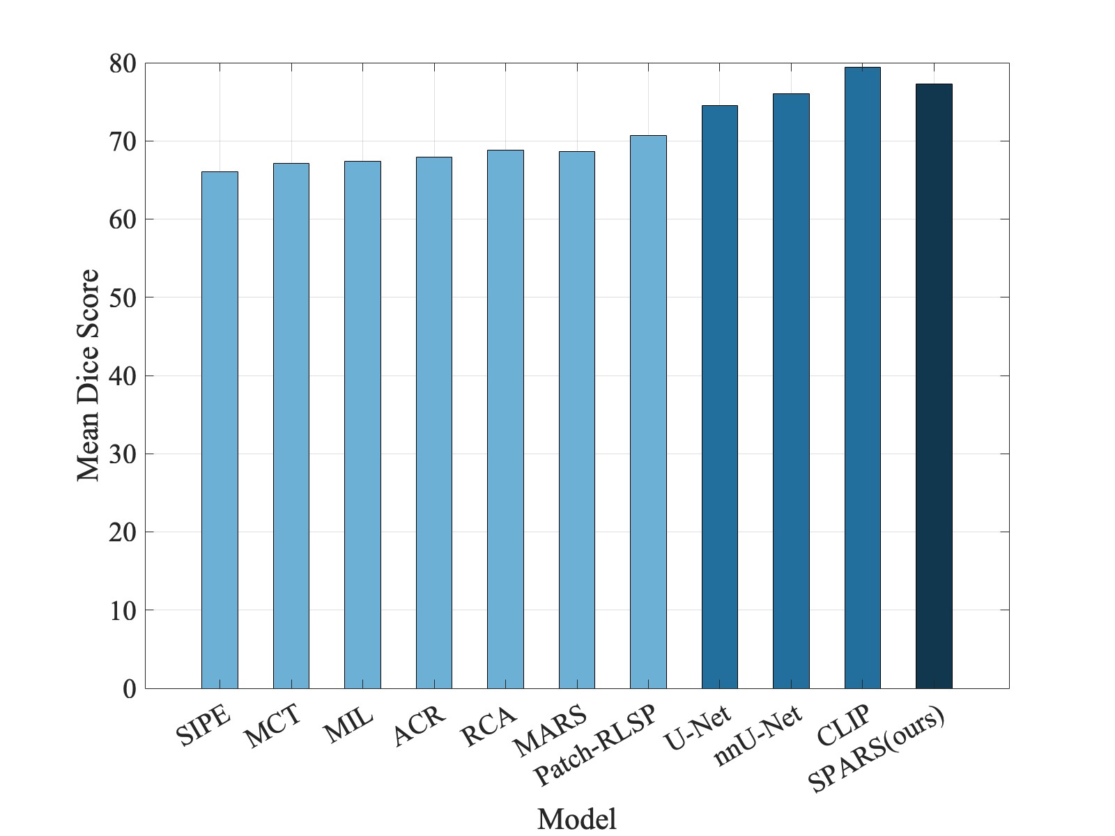
Figure 5: Performance compared to other models for liver tumour segmentation (U-Net, nnU-Net and CLIP are fully-supervised and rest are all weakly-supervised).

4.2.2 Comparisons with fully-supervised methods:

Tab. 1 and Fig. 5 show that our approach outperformed several existing fully-supervised models including U-Net ($\text{Dice}=74.5$) and performed comparably to CLIP which is the current state-of-the-art for the tested task ($\text{Dice}=79.4$) [26], where our method only had 2.5% lower Dice ($\text{Dice}=77.3$). However, the methods compared against, used the full segmentation labels for training which are much more costly to obtain compared to weak labels that are used in our method. Additionally, we only used 24 weak labels for training compared to over 64 full segmentation labels used by other methods. Statistical tests were not conducted due to the absence of standard deviations on reported dice scores for other methods.

4.3 Qualitative results

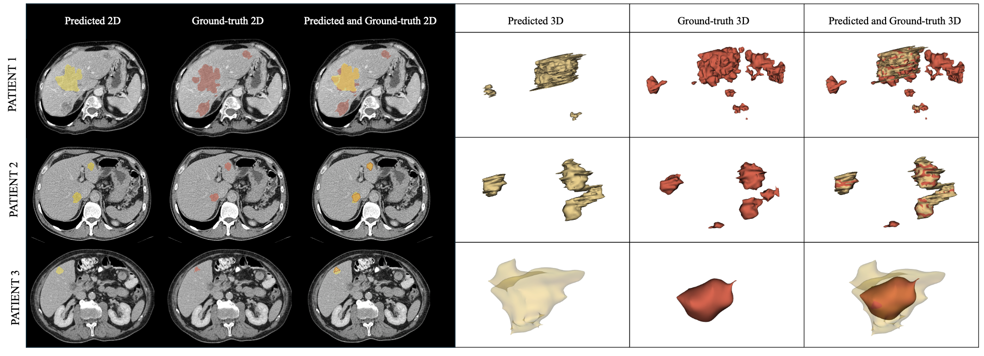
Figure 6: Qualitative examples for a comparison between our predicted segmentations and ground-truth from radiologist annotations.

Fig. 6 shows qualitative examples of predicted and ground truth liver tumour segmentations on patient data. We observed that larger tumours (volume $>10^{3}~\text{mm}^{3}$) were under-segmented (Patient 1) compared to smaller tumours (Patients 2 and 3). We also observed a 24.5% lower average Dice for small tumours compared to their larger counterparts. Luan et al [23] reported similar trends for their liver tumour segmentation framework where smaller tumours (< 0.2 cm) achieved a 60% lower mean dice score ($\text{Dice}=0.32$) than larger tumours.

5 Discussion

We observed a large performance improvement for our method compared to the previous best-performing weakly-supervised method [29] for the same application. Despite both using self-play RL for WSSS, our method enables voxel level probability maps by accumulating the classifier predictions using a moving window (summarised in Sec. 2.4). This enables multiple passes over the same areas to increase segmentation confidence unlike previous patch-based approaches that only allow binary selection or rejection of patches or pixels [29]. This, along with the novel termination condition based on a thresholded classifier score, mean that our framework allows more flexibility in tuning thresholds and parameters for different applications. This application-specific tuning in our flexible framework may be the reason that we observed superior performance compared to recent state-of-the-art methods.

The ablation studies reveal the impact of key hyper-parameters on performance. The performance plateaus after a large enough window size. The performance improvement observed with increasing window size may be due to the fact that as windows become larger their appearance starts to match the appearance of full images. The performance peaks at termination threshold of 0.3, indicating that low thresholds may not be suitable as they may terminate segmentation too early (under-prediction) whereas high thresholds may terminate segmentation too late (over-prediction). The skew of the optimal threshold towards under-prediction may be because of an over representation of cancer-positive classes in the dataset.

Our method performed comparably with fully-supervised approaches despite only using weak labels during training, which are much more cost-effective to obtain compared to voxel-level segmentation labels. This highlights that cost-effective training mechanisms like WSSS may be viable alternatives to fully-supervised learning when data is constrained or of poor quality.

Future investigation could explore alternative reward or termination conditions that allow greater flexibility for application-specific tuning, which may allow even further performance improvements.

6 Conclusion

In this work, we proposed self-play adversarial learning for semantic segmentation (SPARS) where agents compete to localise ROIs. Only weakly supervised labels were utilised to train an object presence classifier, which guides and scores the competition, allowing agents to move windows closer to ROIs. This approach successfully outperformed existing state-of-the-art WSSS models and performed comparably to fully-supervised method which used costly voxel-level segmentations for training. This highlights the cost-effective nature of weakly-supervised training with minimal compromise on performance compared to costly fully-supervised training.

References

- [1] Jiwoon Ahn and Suha Kwak “Learning Pixel-level Semantic Affinity with Image-level Supervision for Weakly Supervised Semantic Segmentation” In Proceedings of the IEEE Computer Society Conference on Computer Vision and Pattern Recognition IEEE Computer Society, 2018, pp. 4981–4990 DOI: 10.1109/CVPR.2018.00523
- [2] Patrick Bilic al. “The Liver Tumor Segmentation Benchmark (LiTS)” In Medical Image Analysis 84 Elsevier, 2023
- [3] Alhanoof Althnian et al. “Impact of dataset size on classification performance: an empirical evaluation in the medical domain” In Applied sciences 11.2 MDPI, 2021, pp. 796
- [4] Nikita Araslanov and Stefan Roth “Single-stage semantic segmentation from image labels” In Proceedings of the IEEE/CVF conference on computer vision and pattern recognition, 2020, pp. 4253–4262
- [5] Liam F Chalcroft et al. “Development and evaluation of intraoperative ultrasound segmentation with negative image frames and multiple observer labels” In Simplifying Medical Ultrasound: Second International Workshop, ASMUS 2021, Held in Conjunction with MICCAI 2021, Strasbourg, France, September 27, 2021, Proceedings 2, 2021, pp. 25–34 Springer
- [6] Qi Chen, Lingxiao Yang, Jianhuang Lai and Xiaohua Xie “Self-supervised Image-specific Prototype Exploration for Weakly Supervised Semantic Segmentation” In Proceedings of the IEEE Computer Society Conference on Computer Vision and Pattern Recognition 2022-June IEEE Computer Society, 2022, pp. 4278–4288
- [7] Andrea Chierici et al. “Vascular liver segmentation: a narrative review on methods and new insights brought by artificial intelligence” In The Journal of international medical research 52.9, 2024
- [8] Dan Ciresan, Alessandro Giusti, Luca Gambardella and Jürgen Schmidhuber “Deep neural networks segment neuronal membranes in electron microscopy images” In Advances in neural information processing systems 25, 2012
- [9] Steffen Czolbe, Kasra Arnavaz, Oswin Krause and Aasa Feragen “Is segmentation uncertainty useful?” In Information Processing in Medical Imaging: 27th International Conference, IPMI 2021, Virtual Event, June 28–June 30, 2021, Proceedings 27, 2021, pp. 715–726 Springer
- [10] Jifeng Dai, Kaiming He and Jian Sun “BoxSup: Exploiting Bounding Boxes to Supervise Convolutional Networks for Semantic Segmentation” In Proceedings of the IEEE International Conference on Computer Vision, 2015 DOI: 10.1109/ICCV.2015.191
- [11] Tobias Heimann et al. “Comparison and Evaluation of Methods for Liver Segmentation from CT datasets” In IEEE Transactions on Medical Imaging 28, 2009, pp. 1251–1265
- [12] Laurent Hermoye et al. “Liver Segmentation in Living Liver Transplant Donors: Comparison of Semiautomatic and Manual Methods1” In Radiology 234.1, 2005, pp. 171–178
- [13] Theodore S. Hong et al. “Interobserver Variability in Target Definition for Hepatocellular Carcinoma With and Without Portal Vein Thrombus: Radiation Therapy Oncology Group Consensus Guidelines” In International journal of radiation oncology, biology, physics 89.4, 2014, pp. 804
- [14] Fabian Isensee et al. “nnU-Net: a self-configuring method for deep learning-based biomedical image segmentation” In Nature Methods 2020 18:2 18 Nature Publishing Group, 2020
- [15] Sanghyun Jo, In-Jae Yu and Kyungsu Kim “Mars: Model-agnostic biased object removal without additional supervision for weakly-supervised semantic segmentation” In Proceedings of the IEEE/CVF International Conference on Computer Vision, 2023, pp. 614–623
- [16] Anna Khoreva et al. “Simple Does It: Weakly Supervised Instance and Semantic Segmentation” In Proceedings - 30th IEEE Conference on Computer Vision and Pattern Recognition, CVPR 2017 2017-January Institute of ElectricalElectronics Engineers Inc., 2016, pp. 1665–1674 DOI: 10.1109/CVPR.2017.181
- [17] Alexander Kolesnikov and Christoph H Lampert “Seed, expand and constrain: Three principles for weakly-supervised image segmentation” In Computer Vision–ECCV 2016: 14th European Conference, Amsterdam, The Netherlands, October 11–14, 2016, Proceedings, Part IV 14, 2016, pp. 695–711 Springer
- [18] Georgios Krokos et al. “Evaluation of manual and automated approaches for segmentation and extraction of quantitative indices from [18F]FDG PET-CT images” In Biomedical Physics & Engineering Express 10.2, 2024, pp. 025007
- [19] Hyeokjun Kweon, Sung Hoon Yoon and Kuk Jin Yoon “Weakly Supervised Semantic Segmentation via Adversarial Learning of Classifier and Reconstructor” In Proceedings of the IEEE Computer Society Conference on Computer Vision and Pattern Recognition IEEE Computer Society, 2023
- [20] Kailu Li et al. “Weakly supervised histopathology image segmentation with self-attention” In Medical Image Analysis 86 Elsevier, 2023
- [21] Di Lin et al. “ScribbleSup: Scribble-Supervised Convolutional Networks for Semantic Segmentation” In Proceedings of the IEEE Computer Society Conference on Computer Vision and Pattern Recognition 2016-December IEEE Computer Society, 2016, pp. 3159–3167 DOI: 10.1109/CVPR.2016.344
- [22] Jie Liu et al. “CLIP-Driven Universal Model for Organ Segmentation and Tumor Detection” In Proceedings of the IEEE International Conference on Computer Vision Institute of ElectricalElectronics Engineers Inc., 2023, pp. 21095–21107 DOI: 10.1109/ICCV51070.2023.01934
- [23] Shunyao Luan et al. “Adaptive Attention Convolutional Neural Network for Liver Tumor Segmentation” In Frontiers in Oncology 11 Frontiers Media S.A., 2021
- [24] Zhiyi Pan et al. “Scribble-Supervised Semantic Segmentation by Uncertainty Reduction on Neural Representation and Self-Supervision on Neural Eigenspace” In Proceedings of the IEEE International Conference on Computer Vision Institute of ElectricalElectronics Engineers Inc., 2021, pp. 7396–7405 DOI: 10.1109/ICCV48922.2021.00732
- [25] Martynas Pocius et al. “Weakly supervised localisation of prostate cancer using reinforcement learning for bi-parametric MR images” In 2024 IEEE International Symposium on Biomedical Imaging (ISBI), 2024, pp. 1–5 IEEE
- [26] Olaf Ronneberger, Philipp Fischer and Thomas Brox “U-net: Convolutional networks for biomedical image segmentation” In Medical image computing and computer-assisted intervention–MICCAI 2015: 18th international conference, Munich, Germany, October 5-9, 2015, proceedings, part III 18, 2015, pp. 234–241 Springer
- [27] Shaheer U Saeed et al. “Active learning using adaptable task-based prioritisation” In Medical Image Analysis 95 Elsevier, 2024, pp. 103181
- [28] Shaheer U Saeed et al. “Guided ultrasound acquisition for nonrigid image registration using reinforcement learning” In Medical Image Analysis 102 Elsevier, 2025, pp. 103555
- [29] Shaheer U. Saeed et al. “Competing for Pixels: A Self-play Algorithm for Weakly-supervised Semantic Segmentation” In IEEE Transactions on Pattern Analysis and Machine Intelligence IEEE Computer Society, 2024
- [30] John Schulman et al. “Proximal policy optimization algorithms” In arXiv preprint arXiv:1707.06347, 2017
- [31] Po Ming Wang et al. “Stereotactic body radiation therapy in hepatocellular carcinoma: Optimal treatment strategies based on liver segmentation and functional hepatic reserve” In Reports of Practical Oncology and Radiotherapy 20.6, 2015, pp. 417–424
- [32] Yunchao Wei et al. “Revisiting Dilated Convolution: A Simple Approach for Weakly- and Semi- Supervised Semantic Segmentation” In Proceedings of the IEEE Computer Society Conference on Computer Vision and Pattern Recognition IEEE Computer Society, 2018, pp. 7268–7277 DOI: 10.1109/CVPR.2018.00759
- [33] Cheng-Chung Wu et al. “Occlusion of Hepatic Blood Inflow for Complex Central Liver Resections in Cirrhotic Patients: A Randomized Comparison of Hemihepatic and Total Hepatic Occlusion Techniques” In Archives of Surgery 137.12, 2002, pp. 1369–1376
- [34] Lian Xu et al. “Multi-class Token Transformer for Weakly Supervised Semantic Segmentation” In Proceedings of the IEEE Computer Society Conference on Computer Vision and Pattern Recognition 2022-June IEEE Computer Society, 2022, pp. 4300–4309
- [35] Weixi Yi et al. “Boundary-RL: Reinforcement learning for weakly-supervised prostate segmentation in TRUS images” In International Workshop on Machine Learning in Medical Imaging, 2023, pp. 277–288 Springer
- [36] Tianfei Zhou, Meijie Zhang, Fang Zhao and Jianwu Li “Regional Semantic Contrast and Aggregation for Weakly Supervised Semantic Segmentation” In Proceedings of the IEEE Computer Society Conference on Computer Vision and Pattern Recognition 2022-June IEEE Computer Society, 2022, pp. 4289–4299