GraSS: Scalable Influence Function with Sparse Gradient Compression

Abstract

Gradient-based data attribution methods, such as influence functions, are critical for understanding the impact of individual training samples without requiring repeated model retraining. However, their scalability is often limited by the high computational and memory costs associated with per-sample gradient computation. In this work, we propose GraSS, a novel gradient compression algorithm and its variants FactGraSS for linear layers specifically, that explicitly leverage the inherent sparsity of per-sample gradients to achieve sub-linear space and time complexity. Extensive experiments demonstrate the effectiveness of our approach, achieving substantial speedups while preserving data influence fidelity. In particular, FactGraSS achieves up to $165\%$ faster throughput on billion-scale models compared to the previous state-of-the-art baselines. Our code is publicly available at https://github.com/TRAIS-Lab/GraSS.

1 Introduction

Data attribution aims to measure the impact of individual training samples on a machine learning model and has been widely applied to data-centric problems in modern AI, such as data curation (Koh and Liang, 2017), fact tracing (Lin et al., 2024), and data compensation (Deng et al., 2024b). There are two major categories of data attribution methods, gradient-based and retraining-based (Hammoudeh and Lowd, 2024). The former category, such as influence functions (Koh and Liang, 2017) and its variants, has gained increasing popularity in large-scale applications as it does not require costly model retraining. One common feature of gradient-based methods is their reliance on the per-sample gradient—the gradient of the loss with respect to model parameters for each individual data point—to capture the local sensitivity of the model with respect to each training sample, providing a fine-grained understanding of data influence.

However, gradient-based methods still face significant scalability challenges for very large models, such as large language models (LLMs). Specifically, computing and storing per-sample gradients for a model with $n$ training samples and $p$ parameters requires $O(np)$ memory, creating a severe bottleneck for large-scale models. To address this, recent work has explored compressing these high-dimensional gradients into lower-dimensional representations, reducing memory requirements to $O(nk)$ for a target compression dimension $k\ll p$ (Wojnowicz et al., 2016; Park et al., 2023; Choe et al., 2024). However, this compression often introduces additional computational overhead, as the most common approach—random matrix projection with the Johnson-Lindenstrauss (JL) guarantee—requires dense matrix multiplications, resulting in an overall time complexity of $O(nkp)$ and an additional $O(kp)$ memory overhead for the projection matrix itself.

To overcome these limitations, more specialized approaches have been proposed. For example, the Fast Johnson-Lindenstrauss Transform (FJLT) used in Trak’s official implementation (Park et al., 2023) exploits structured random matrices, eliminating the need to store the full projection matrix and reduces the projection time to $O(p\log p+k\log p)$. Alternatively, recent work by Choe et al. (2024) proposed LoGra that leverages the Kronecker product structure of gradients in linear layers, reducing projection time to $O(\sqrt{pk})$ for each data via a factorized matrix approach. However, these methods are often designed for general inputs and do not fully exploit the unique sparsity structures present in per-sample gradients.

In this paper, we push the boundaries of these state-of-the-art (SOTA) gradient compression methods by proposing a novel, two-stage gradient compression algorithm called GraSS (Gradient Sparsification and Sparse-projection), that achieves sub-linear space and time complexity by explicitly leveraging the inherent sparsity of per-sample gradients. Our contributions are as follows:

1. We identify two critical sparsity properties in per-sample gradients and leverage these to develop a gradient compression algorithm, GraSS, that reduces both space and time complexity from $O(pk)$ to $O(k^{\prime})$, where $k^{\prime}$ is a tunable hyperparameter in the range $[k,p]$.

2. We further derive a practically efficient variant of GraSS for linea layers, called FactGraSS, which exploits the gradient structures for linear layers, achieving a time and space complexity of $O((k^{\prime})^{2})$, where $k^{\prime}$ is a tunable hyperparameter in the range $[\sqrt{k},\sqrt{p}]$, without the need to ever materalizing the full gradients. In most practical scenarios, FactGraSS is not only asymptotically, but also practically faster than the previous SOTA baseline, LoGra.

3. Through extensive data attribution experiments, we demonstrate that our approach achieves several orders of magnitude speedup while maintaining competitive performance on standard evaluation metrics. Additionally, we show its effectiveness on billion-scale language models, Llama-3.1-8B-Instruct, where FactGraSS is up to $165\%$ faster in terms of compression throughput, and the influential data points identified by FactGraSS also share qualitatively meaningful characteristics with the query data point.

2 Preliminary

We first introduce the influence function with some remarks on the practical implementation. Then, we show how random projection can be used together with the influence function.

2.1 Influence function

Given a dataset $D=\{z_{i}\in\mathbb{R}^{d}\}_{i=1}^{n}$, consider a model parametrized by $\hat{\theta}\in\mathbb{R}^{p}$ that this trained on the dataset $D$ with a loss function $\ell\colon\mathbb{R}^{d}\times\mathbb{R}^{p}\to\mathbb{R}$ via empirical risk minimization: $\hat{\theta}=\operatorname*{arg\,min}_{\theta\in\mathbb{R}^{p}}\frac{1}{n}\sum_{i=1}^{n}\ell(z_{i};\theta)$. Under this setup, the influence function (Koh and Liang, 2017) can be theoretically derived; essentially, it gives an estimation on every training data $z_{i}$’s “influence” $\mathcal{I}(z_{i},z_{\text{test}})$ of the test loss $\ell(z_{\text{test}};\hat{\theta})$ of a given test data $z_{\text{test}}$ when $z_{i}$ is removed from $D$ as

$$\mathcal{I}(z_{i},z_{\text{test}})\coloneqq\nabla_{\theta}\ell(z_{\text{test}};\hat{\theta})^{\top}H_{\hat{\theta}}^{-1}\nabla_{\theta}\ell(z_{i};\hat{\theta}),$$

where $H_{\hat{\theta}}=\frac{1}{n}\sum_{i=1}^{n}\nabla^{2}_{\theta}\ell(z_{i},\hat{\theta})$ is the empirical Hessian. As $H_{\hat{\theta}}\in\mathbb{R}^{p\times p}$ and computing it requires higher-order differentiation for every training data, several approximation algorithms aim to mitigate this. One famous approximation is the Fisher information matrix (FIM) (Fisher, 1922) approximation $H_{\hat{\theta}}\approx\mathbb{E}_{z}[\nabla_{\theta}\ell(z;\hat{\theta})\nabla_{\theta}\ell(z;\hat{\theta})^{\top}]$ for model trained with the negative log-likelihood objective. FIM only involves the first-order gradient, which is also needed in the calculation of $\mathcal{I}$, and hence is a popular and efficient approximation. Given this, people realize that an efficient way to compute the influence function is to divide the computation into two stages (Lin et al., 2024; Choe et al., 2024):

1. Cache stage: 1.) compute all per-sample gradients $g_{i}\coloneqq g_{z_{i}}\coloneqq\nabla_{\theta}\ell(z_{i};\hat{\theta})$, 2.) construct the FIM $F_{\hat{\theta}}\coloneqq\frac{1}{n}\sum_{i=1}^{n}g_{i}g_{i}^{\top}$, 3.) perform inverse FIM-vector-product (iFVP) via $\widetilde{g}_{i}\coloneqq F_{\hat{\theta}}^{-1}g_{i}$ for all $z_{i}$’s.

2. Attribute stage: For a query data $z_{\text{test}}$, 1.) compute its per-sample gradient $g_{\text{test}}\coloneqq\nabla_{\theta}\ell(z_{\text{test}};\hat{\theta})$, 2.) compute all-pair-inner-product between $g_{\text{test}}$ and $\{\widetilde{g}_{i}\}_{i=1}^{n}$ as $\mathcal{I}(z_{i},z_{\text{test}})=\langle g_{\text{test}},\widetilde{g}_{i}\rangle$ for all $z_{i}$’s.

The bottleneck of this pipeline is the cache stage, since the problem for the attribute stage is the well-studied vector inner product search, where numerous optimization techniques have been studied in the vector database community. On the other hand, iFVP remains a challenging task due to the matrix inversion of quadratic model size, where in most cases, even materializing FIM is infeasible.

2.2 Random projection

Despite multiple attempts to accelerate influence function from various angles, one of the most naive and simple strategies, Random (Wojnowicz et al., 2016; Schioppa et al., 2022; Park et al., 2023), remains practically relevant and achieves SOTA attribution results. Random leverages sketching (random projection) techniques by replacing each per-sample gradient $g_{i}\in\mathbb{R}^{p}$ with $g^{\prime}_{i}\coloneqq Pg_{i}\in\mathbb{R}^{k}$, where $P\in\mathbb{R}^{k\times p}$ is a random projection matrix for some $k\ll p$. This subsequently leads to the projected FIM approximation $F^{\prime}_{\hat{\theta}}\coloneqq PF_{\hat{\theta}}P^{\top}=\mathbb{E}_{z}[(g^{\prime}_{z}\cdot(g^{\prime}_{z})^{\top})]\in\mathbb{R}^{k\times k}$, i.e., a restriction of $F_{\hat{\theta}}$ to the subspace spanned by the rows of $P$. The theoretical merits of Random largely come from the well-known Johnson-Lindenstrauss lemma (Johnson, 1984), which states that for $P$ drawn appropriately, e.g., $P_{ij}\overset{\text{i.i.d.}}{\sim}\mathcal{N}(0,1)$ or $\mathcal{U}(\{\pm 1\})$ for all $i,j$, with high probability, the pair-wise distance $\lVert g_{i}-g_{j}\|$ between any two $g_{i}$ and $g_{j}$ will be preserved up to $1\pm\epsilon$ factor after the projection, whenever $k=O(\epsilon^{-2}\log n)$. While this does not fully justify whether the inner product between a projected per-test-sample gradient $g^{\prime}_{\text{test}}$ and the “conditioned” projected per-train-sample gradient $\widetilde{g}^{\prime}_{i}\coloneqq(F^{\prime}_{\hat{\theta}})^{-1}g^{\prime}_{i}$ will be preserved (see Section˜A.2 for an in-depth discussion), Random remains to be one of the strongest baselines to date and is practically appealing due to its simplicity.

Remark 2.1.

We follow the same notational convention in the rest of the paper: the per-sample gradient is denoted as $g$, compressed per-sample gradient is denoted as $g^{\prime}$, and finally the (FIM) preconditioned per-sample gradient is denoted as $\widetilde{g}$. The latter two can be used together, i.e., $\widetilde{g}^{\prime}$ denotes the projected per-sample gradient precondition by $(F_{\hat{\theta}}^{\prime})^{-1}$, the inverse of the projected FIM.

Computational-wise, Random accelerates iFVP significantly as the matrix inversion complexity scales down from $O(p^{2})$ to $O(k^{2})$. In terms of the projection overhead, the matrix-based projection method requires $O(kp)$ overhead per projection. Trak (Park et al., 2023) leverages the fast Johnson-Lindenstrauss transform (FJLT) (Ailon and Chazelle, 2009; Fandina et al., 2023) that has a similar theoretical guarantee as the random matrix-based projection to achieve a speed up of $O(p\log p+k\log p)$. Another line of work by Choe et al. (2024) called LoGra exploits the gradient structure of linear layers and factorizes the projection accordingly, reducing the problem size quadratically. In general, with suitable and reasonable parameter choice, the computational complexity goes down from $O(kp)$ to $O(\sqrt{kp})$, achieving the SOTA efficiency and attribution quality.

3 GraSS: Gradient Sparsification and Sparse Projection

In this section, we first explore two key sparsity properties in per-sample gradients (Sections˜3.1 and 3.2) and propose efficient compression methods for each. Combining them, we present GraSS and its variant FactGraSS (Section˜3.3), which beat the previous SOTA data attribution algorithms.

3.1 Per-sample gradient sparsity

Modern deep learning models often induce highly sparse per-sample gradients, especially when using popular activation functions like ReLU (Nair and Hinton, 2010). To see this, consider the gradient of the first read-in linear layer with a weight matrix $W\in\mathbb{R}^{d^{\prime}\times d}$ and ReLU activations. Then given a sample $z\in\mathbb{R}^{d}$, the output is $h=\operatorname{ReLU}(Wz)$. Since $\operatorname{ReLU}(x)=\max(0,x)$ sets all negative pre-activations to zero, naturally creating sparse activations. This sparsity propagates to the gradient computations via the chain rule, resulting in gradients with numerous zero entries. This property is not unique to ReLU and extends to many other activation functions that exhibit similar behavior.

Remark 3.1.

This sparsity is unique to per-sample gradients: for mini-batch gradients $\sum_{i\in B}g_{i}/\lvert B\rvert$, the sparsity pattern differs for individual $g_{i}$ and will be destroyed when adding together.

Given the inherently sparse nature of these gradients, it is natural to consider other compression methods that can take advantage of the input sparsity, since both the traditional dense random projection methods and the more efficient, explored projection method, FJLT, can not.

Sparse Johnson-Lindenstrauss Transform.

A natural candidate for efficient gradient projection is the sparse Johnson-Lindenstrauss transform (SJLT) (Dasgupta et al., 2010; Kane and Nelson, 2014), which significantly reduces the computational cost by sparsifying the projection matrix. To understand SJLT, it is useful to revisit the standard matrix-based projection approach, which relies on matrix-vector multiplication. Given a projection matrix $P\in\mathbb{R}^{k\times p}$ and an input vector $g\in\mathbb{R}^{p}$ to be projected, the product $Pg$ can be computed as $g^{\prime}=Pg=\sum_{j=1}^{p}g(j)P_{\colon j}$, where the $j^{\text{th}}$ term represents the $j^{\text{th}}$ column $P_{\colon j}$ of $P$ scaled by the $j^{\text{th}}$ entry $g(j)$ of $g$. In the case of a dense Rademacher projection matrix (entries being $\pm 1$), this requires $O(pk)$ computation for both constructing $g(j)P_{\colon j}$ and summing them. This dense projection process is illustrated in Figure˜1(a), where each arrow corresponds to multiplying a single entry of $g$ by either $+1$ or $-1$.

((a)) Dense Rademacher projection.

((b)) Sparse Rademacher projection ($s=2$).

Figure 1: Illustration of dense projection and SJLT for Rademacher entries.

From this perspective, the SJLT arises naturally: by effectively “dropping” edges in the computation graph, e.g., Figure˜1(b), we significantly reduce the computational burden. Specifically, Dasgupta et al. (2010) and Kane and Nelson (2014) demonstrated that retaining only $s=o_{\epsilon}(k)$ out of the k possible non-zero connections for each projected dimension still preserves the essential properties required by the Johnson-Lindenstrauss lemma. This approach, which we denote as $\operatorname{\textnormal{{SJLT}}}_{k}(\cdot)$, reduces both the time and space complexity to $O(ps)$, where $s=o_{\epsilon}(k)$ is much smaller than $k$. In practice, we often set $s=1$ to further optimize for speed.

Moreover, if the input vector $g$ is itself sparse, the computational cost can be further reduced. Specifically, for a dense matrix projection, the complexity becomes $O(k\operatorname{nnz}(g))$, and for SJLT, this drops to $O(s\operatorname{nnz}(g))$, where $\operatorname{nnz}(g)\coloneqq\lVert g\rVert_{0}$ denotes the number of non-zero entries in $g$.

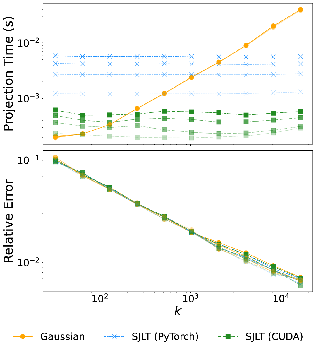
Figure 2: Benchmark of different projections with dimension from $p=131,072$ to various $k$ under several sparsity levels (distinguished by opacity).

Despite these theoretical advantages, practical implementations of SJLT face critical performance challenges such as thread contention and irregular memory access patterns. While the latter is due to the nature of SJLT, the former occurs because multiple threads may attempt to write to the same entry in the output vector, causing race conditions that degrade performance, especially when the target dimension $k$ is small. These are especially critical when implementing in general-purpose libraries like PyTorch. Moreover, the default matrix multiplication algorithms in PyTorch are highly hardware-optimized (e.g., cache-friendly memory layouts and fused multiply-accumulate instructions), often outperforming any similar multiplication algorithms when the problem size is small.

To address these issues, we developed a custom SJLT CUDA kernel that optimizes memory access patterns and minimizes thread contention to better exploit the underlying hardware capabilities. This kernel significantly reduces the overhead compared to its PyTorch implementation counterpart, resulting in substantial performance gains. As shown in Figure˜2, for SJLT with $s=1$, our CUDA implementation outperforms the highly optimized dense matrix multiplications for small projection dimensions ($k\geq 256$), while retaining the scaling advantages of SJLT with respect to input sparsity. In contrast, dense Gaussian projections exhibit a clear dependency on both $k$ and the number of non-zero entries, making them less efficient in practice.

Remark 3.2.

The complexity of SJLT 1.) scales with the input sparsity, and 2.) is independent of the target dimension $k$, both of which are critical for efficient gradient compression. Specifically, 1.) per-sample gradients are naturally sparse, and 2.) larger $k$ generally improves the fidelity of data attribution, which is more desirable. These make SJLT a natural fit for gradient compression.

3.2 Effective parameter sparsity

While SJLT effectively reduces the computational overhead and takes advantage of the sparsity structure of the input, it still scales linearly with the potentially large input dimensionality $p$. We now explore a more aggressive compression that achieves sub-linear complexity by directly exploiting the inherent effective parameter sparsity in neural networks. We term this approach as sparsification.

3.2.1 Random Mask

Modern deep learning models often exhibit a high degree of parameter redundancy, where only a small fraction of the weights significantly contribute to the model’s final performance (Han et al., 2016; Frankle and Carbin, 2019). In a similar vein, in the distributed training community, it is observed that the majority of gradient updates are redundant, allowing for substantial compression without significant impact on model accuracy (Lin et al., 2018; Aji and Heafield, 2017). This suggests that many parameters can be safely ignored without substantial loss in accuracy. Inspired by this observation, a simple yet surprisingly effective sparsification algorithm, Random Mask, randomly selects a small subset from the $p$ input dimensions to form a compressed representation.

Formally, the Random Mask ($\operatorname{\textnormal{{RM}}}_{k}(\cdot)$) involves selecting a random subset of $k$ dimensions from the original $p$-dimensional gradient vector, effectively extracting a length-$k$ sub-vector. This can also be viewed as a random projection onto the standard basis of a randomly chosen $k$-dimensional Euclidean subspace, i.e., $g^{\prime}=Mg$ where $M\in\mathbb{R}^{k\times p}$ is a sparse binary selection matrix with exactly one (non-repetitive) non-zero entry per row, corresponding to the randomly chosen dimensions.

At first glance, $\operatorname{\textnormal{{RM}}}_{k}$ may seem overly aggressive, as it discards a substantial amount of information. However, empirical evidence suggests that this method can still yield non-trivial attribution performance, especially when the underlying gradient distribution is sparse or when the model is over-parameterized. Moreover, the extreme simplicity of this approach makes it highly efficient, with a computational cost of just $O(k)$, achieving a sub-linear complexity w.r.t. $p$.

3.2.2 Selective Mask

Building on the idea of Random Mask, we introduce a more structured approach, Selective Mask ($\operatorname{\textnormal{{SM}}}_{k}(\cdot)$), which aims to selectively retain the most important parameters based on a simple, yet effective, data-driven optimization. Inspired by recent work on identifying influential model parameters (He et al., 2025), Selective Mask introduces a small but meaningful optimization overhead to improve the fidelity of the compressed representation. Formally, given a training set $\{z_{i}\}_{i=1}^{n}$, we define the selective masking problem as the following unconstrained optimization task:

$$S^{\ast}=\operatorname*{arg\,max}_{S\in\mathbb{R}^{p}}\mathbb{E}_{z_{\text{test}}}\left[\operatorname{corr}\left((\langle g_{i},g_{z_{\text{test}}}\rangle)_{i=1}^{n},(\langle\hat{g}_{i},\hat{g}_{z_{\text{test}}}\rangle)_{i=1}^{n}\right)\right]-\lambda\|\sigma(S)\|_{1},$$ (1)

where $\hat{g}_{i}=\sigma(S)\odot g_{i}\in\mathbb{R}^{p}$ is the (soft-)masked $g_{i}$, $\odot$ denotes the element-wise product, and $\sigma(\cdot)\in(0,1)$ is the sigmoid function. The first term of the objective encourages the average correlation between the original and masked gradients’ GradDot attribution scores (Charpiat et al., 2019), a widely used and computationally efficient approximation of the influence function. The second term, an $\ell_{1}$ regularization penalty, promotes sparsity by pushing $\sigma(S)$ towards a binary mask.

Once the optimal $S^{\ast}$ is obtained after solving Eq.​˜1, the final binary mask $M\in\{0,1\}^{k\times p}$ can be extracted by thresholding the sigmoid outputs with $k=\sum_{j=1}^{p}\mathbbm{1}_{\sigma(S^{\ast})_{j}\geq 0.5}$ is the number of selected dimensions. Formally, one can obtain the explicit mask matrix $M$ via solving $\langle M_{\colon j},1_{k}\rangle=\mathbbm{1}_{\sigma(S^{\ast})j\geq 0.5}$, but the actual implementation is simply an index extraction for all $j$ for $\mathbbm{1}_{\sigma(S^{\ast})_{j}\geq 0.5}$.

This formulation avoids the exponential complexity of directly optimizing over discrete binary masks, as the continuous nature of $S$ allows for efficient, first-order gradient-based optimization. While it incurs a one-time overhead for solving the optimization problem, this method provides a more principled approach to mask selection by directly targeting a widely used surrogate data attribution score, making it a natural extension of the Random Mask approach.

3.3 GraSS & FactGraSS: Multi-stage compression

We now formally introduce GraSS and FactGraSS, an integration of the proposed approaches by combining the sparse projection (Section˜3.1) and also sparsification techniques (Section˜3.2).

3.3.1 GraSS: Sparsify first, sparse projection next

Recall that the time complexity of SJLT with $s=1$ is $O(p)$ where $p$ is the input dimension, while for both sparsification techniques are $O(k)$ where $k$ is the target sparsification dimension. A natural idea is to employ a two-stage compression: Given an input and target compression dimension $k\ll p$,

1. Sparsification: sparsify the input to an intermediate dimension $k^{\prime}$ sub-vector with $k<k^{\prime}\ll p$.

2. Sparse projection: then apply SJLT to the sub-vector of dimension $k^{\prime}$ with the target dimension $k$.

Notation-wise, we write $\operatorname{\textnormal{{SJLT}}}_{k}\circ\operatorname{\textnormal{{RM}}}_{k^{\prime}}$ (or $\operatorname{\textnormal{{SJLT}}}_{k}\circ\operatorname{\textnormal{{SM}}}_{k^{\prime}}$ in the case of Selective Mask). Intuitively, as sparsification achieves non-trivial attribution performance, we expect that the attribution performance will increase with $k^{\prime}$; subsequently, sketching these $k^{\prime}$ dimensions with SJLT without losing the pair-wise distance information further compresses the result down to the target dimension.

This simple Gradient Sparsification and Sparse projection (GraSS) compression method leads to an sub-linear time complexity $O(k^{\prime}+k^{\prime})=O(k^{\prime})$ to the input dimension $p$, since the runtime of SJLT depends only on its input dimension, which is now sparsified to $k^{\prime}$ from $p$. In the extreme cases when $k^{\prime}=p$, GraSS reduces to vanilla SJLT; while when $k^{\prime}=d$, GraSS reduces to sparsification.

3.3.2 FactGraSS: Exploiting layer-wise gradient factorization structure

In addition to FIM approximation, influence function on large-scale models often leverages the layer-wise independence assumption by approximating FIM as a block-diagonal matrix, ignoring parameter interactions across layers. Specifically, this approach decomposes the FIM as $\operatorname{diag}\{F_{\hat{\theta}_{1}},\cdots,F_{\hat{\theta}_{L}}\}$ for an $L$-layer neural network, where each block $F_{\hat{\theta}_{l}}$ is a compressed approximation for the $l^{\text{th}}$ layer’s parameters $\hat{\theta}_{l}$, defined as $F_{\hat{\theta}_{l}}=\mathbb{E}_{z}[\nabla_{\theta_{l}}\ell(z;\hat{\theta})\nabla_{\theta_{l}}\ell(z,\hat{\theta})^{\top}]$. Coupling this trick with gradient compression, the projection problem’s effective size is significantly reduced.

However, this renders a critical challenge for GraSS to demonstrate practical speedup via a direct replacement of each of these highly factorized compression sub-problems, since SJLT suffers from small problem sizes (Section˜3.1). Moreover, recent techniques such as LoGra (Choe et al., 2024) further reduce the compression problem size of each compression task via gradient factorization, making it difficult to integrate GraSS with these SOTA methods to achieve a further speedup.

This motivates the need for a specialized adaptation of GraSS that can effectively exploit a similar gradient factorization structure. To this end, we propose FactGraSS, which explicitly incorporates this factorization structure to achieve even greater efficiency in gradient compression.

Recap on LoGra.

To motivate and understand the practical difficulties we must avoid, we first introduce LoGra. Formally, LoGra exploits the factorized structure of linear layer’s gradients: given a sequential input $z^{\text{in}}\in\mathbb{R}^{d_{\text{in}}\times T}$ of length $T$ and output (pre-activations) $z^{\text{out}}\in\mathbb{R}^{d_{\text{out}}\times T}$ to a linear layer with a weight matrix $W\in\mathbb{R}^{d_{\text{out}}\times d_{\text{in}}}$ such that $z^{\text{out}}=Wz^{\text{in}}$, we have

$$\frac{\partial\ell(z^{\text{in}};\hat{\theta})}{\partial W}=\frac{\partial\ell(z^{\text{in}};\hat{\theta})}{\partial z^{\text{out}}}\frac{\partial z^{\text{out}}}{\partial W}=\frac{\partial\ell(z^{\text{in}};\hat{\theta})}{\partial z^{\text{out}}}{z^{\text{in}}}^{\top}\iff\operatorname{vec}(\mathcal{D}W)=\sum_{t=1}^{T}z^{\text{in}}_{\colon t}\otimes\mathcal{D}z^{\text{out}}_{\colon t},$$ (2)

where we write $\nabla_{v}\ell(z^{\text{in}};\hat{\theta})$ as $\mathcal{D}v$ for any $v$. LoGra then leverages this Kronecker-product structure of $\operatorname{vec}(\mathcal{D}W)$ and assumes the projection matrix $P$ has a similar structure and hence factories, i.e.,

$$P\operatorname{vec}(\mathcal{D}W)\coloneqq(P_{\text{in}}\otimes P_{\text{out}})\operatorname{vec}(\mathcal{D}W)=\sum_{t=1}^{T}(P_{\text{in}}z^{\text{in}}_{\colon t})\otimes(P_{\text{out}}\mathcal{D}z^{\text{out}}_{\colon t}),$$ (3)

where $P_{\text{in}}\in\mathbb{R}^{k_{\text{in}}\times d_{\text{in}}}$, $P_{\text{out}}\in\mathbb{R}^{k_{\text{out}}\times d_{\text{out}}}$, and $P=P_{\text{in}}\otimes P_{\text{out}}\in\mathbb{R}^{(k_{\text{in}}k_{\text{out}})\times(d_{\text{in}}d_{\text{out}})}$, giving a final compression dimension of $k=k_{\text{in}}k_{\text{out}}$. We see that to compute $P\operatorname{vec}(\mathcal{D}W)$:

• forward pass on $z_{i}$ and backward pass on $\ell(z_{i};\hat{\theta})$ will give $z^{\text{in}}$ and $\mathcal{D}z^{\text{out}}$ for every linear layer;

• only two smaller projection problems of size $k_{\text{in}}\times d_{\text{in}}$ and $k_{\text{out}}\times d_{\text{out}}$ are needed, instead of to project the entire gradient, which is of size $(k_{\text{in}}k_{\text{out}})\times(d_{\text{in}}d_{\text{out}})=kp$;

• in addition, the actual gradient of the layer is never materialized (which will require computing Eq.​˜2, $O(Td_{\text{in}}d_{\text{out}})$), only the projected gradient is materialized at the end ($O(Tk_{\text{in}}k_{\text{out}})$).

Notation-wise, as $P_{\text{in}}$ and $P_{\text{out}}$ are default to Gaussian projection (Choe et al., 2024), we write LoGra as $\operatorname{\textnormal{{Gauss}}}_{k_{\text{in}}\otimes k_{\text{out}}}$, where $\otimes$ indicates that the projection is done in a factorized manner. Assuming $d_{\text{in}}\approx d_{\text{out}}$ and choosing $k_{\text{in}}\approx k_{\text{out}}$ results in a speedup from $O(kp)$ to $O(\sqrt{kp})$ per projection.

Bottlenecks of integrating GraSS with LoGra.

In general, one can change the Gaussian matrices used in LoGra to other compression methods. However, a trivial integration by replacing them with GraSS will not lead to a practical speed up, since now each compression problem size is reduced, and increasing it will blow up the FIM size not quadratically, but quartically: if $\hat{k}\coloneqq k_{\text{in}}=k_{\text{out}}\geq 256$, the resulting compressed gradient of this layer will be of size $k=\hat{k}^{2}\geq 65536$, which leads to a projected FIM of size $(\hat{k}^{2})^{2}$, which is greater than $4.3$ billions. Storing such a matrix is challenging, let alone computing its inverse. In most of the practical scenarios, $\hat{k}=64$, where SJLT is several times slower than the baseline dense Gaussian projection (Figure˜2), making a direct integration of GraSS with LoGra challenging.

A natural idea to mitigate this issue is to not factorize the projection: by first constructing the gradients of the layer via Eq.​˜2, we can perform GraSS with a compression dimension target being $k=\hat{k}^{2}$, which is often above the $256$ threshold. However, this requires materializing the gradients explicitly, which blows up the space and time complexity to $O(d_{\text{in}}d_{\text{out}})=O(p)$ compared to LoGra.

Factorized GraSS.

To bypass the bottlenecks, we propose Factorized GraSS (FactGraSS) that exploits the Kronecker-product structure that achieves SOTA efficiency. Specifically, FactGraSS operates in three stages: Given a target compression dimension $k=\hat{k}^{2}\ll p$, after a forward pass on $z_{i}$ and a backward pass on $\ell(z_{i};\hat{\theta})$, for $z_{i}^{\text{in}}$ and $\mathcal{D}z_{i}^{\text{out}}$ from each linear layer,

1. Sparsification: sparsify both $z_{i}^{\text{in}}$ and $\mathcal{D}z_{i}^{\text{out}}$ to an intermediate dimension $k^{\prime}$ where $\hat{k}\leq k^{\prime}\ll\sqrt{p}$;

2. Reconstruction: construct the “sparsified gradient” of dimension $(k^{\prime})^{2}$ via Eq.​˜3, i.e., Kronecker product between the sparsified $z_{i}^{\text{in}}$ and the sparsified $\mathcal{D}z_{i}^{\text{out}}$;

3. Sparse projection: apply SJLT to the sparsified gradient of dimension $(k^{\prime})^{2}$ with the target dimension $k=\hat{k}^{2}$.

Notation-wise, we write $\operatorname{\textnormal{{SJLT}}}_{k^{2}}\circ\operatorname{\textnormal{{RM}}}_{k^{\prime}\otimes k^{\prime}}$ (or $\operatorname{\textnormal{{SJLT}}}_{k^{2}}\circ\operatorname{\textnormal{{SM}}}_{k^{\prime}\otimes k^{\prime}}$ in the case of Selective Mask), where we use $\otimes$ to indicate that the sparsification is done in a factorized manner, and $k^{2}$ signifies that the sparse projection is performed with a large, non-factorized target dimension $k^{2}$.

Intuitively, FactGraSS resolves the two difficulties by 1.) avoid reconstructing the full gradient via sparsification, and 2.) avoid overly small target projection for SJLT via reconstruction. In terms of complexity, sparsification takes $O(k^{\prime})$, and reconstruction takes $O((k^{\prime})^{2})$ for performing the Kronecker product between two vectors of size $k^{\prime}$, and finally sparse projection takes $O((k^{\prime})^{2})$, the size of the input sparsified gradient, giving an overall time and space complexity of $O((k^{\prime})^{2})$.

Remark 3.3.

Since $k^{\prime}\in[\sqrt{k},\sqrt{p}]$, GraSS’s complexity $O(k^{\prime})$ for $k^{\prime}\in[k,p]$ is indeed comparable with $O((k^{\prime})^{2})$ for FactGraSS. However, in contrast to GraSS, FactGraSS does not require materializing the full gradient, providing a further advantage in the case of linear layers.

Compared to LoGra, which has a complexity of $O(\sqrt{kp})=O(\hat{k}\sqrt{p})$, for $k^{\prime}=c\hat{k}$ with some $c\geq 1$, FactGraSS is theoretically faster than LoGra if $(k^{\prime})^{2}\leq\hat{k}\sqrt{p}$, or equivalently,

$$(k^{\prime})^{2}=c^{2}\hat{k}^{2}\leq\hat{k}\sqrt{p}\iff c^{2}\leq\sqrt{p}/\hat{k}\iff c\leq\sqrt[4]{p/k}.$$ (4)

In practice, it is easy to satisfy Eq.​˜4 with a large enough $c$ that achieves competitive attribution performance while having a significant speedup compared to other baselines.

4 Experiment

In this section, we evaluate the effectiveness of GraSS and FactGraSS in terms of accuracy and efficiency. Specifically, in Section˜4.1, we first perform the standard counterfactual evaluations to quantitatively study the data valuation accuracy of GraSS and FactGraSS on small-scale setups. Then, we scale FactGraSS to a billion-scale model and billion-token dataset, where we investigate the qualitative accuracy and memory/compute efficiency in Section˜4.2. Further experimental details such as hyperparameters and compute resources can be found in Section˜B.1.

4.1 Quantitative accuracy via counterfactual evaluation

We assess the quantitative accuracy of data attribution algorithms using the widely adopted linear datamodeling score (LDS) (Park et al., 2023), a counterfactual evaluation method. While LDS relies on the additivity assumption, which is known to be imperfect (Hu et al., 2024), it remains a valuable evaluation metric for data attribution. All the quantitative experiments are conducted on one NVIDIA A40 GPU with 48 GB memory, and other details can be found in Section˜B.2.

GraSS with Trak.

We apply GraSS on one of the SOTA data attribution algorithms (in terms of attribution quality), Trak (Park et al., 2023), with the implementation from the dattri library (Deng et al., 2024a). To validate the effectiveness of our sparsification and sparse projection methods, we conduct an ablation study on a simple 3-layer MLP trained on MNIST (LeCun, 1998). As shown in Table˜1(a), even a standalone Random Mask achieves non-trivial LDS results, while Selective Mask improves the performance further. Additionally, the sparse projection SJLT significantly outperforms baselines like FJLT and Gaussian projection in both efficiency and LDS accuracy.

We evaluate GraSS on more complex models: 1.) ResNet9 (He et al., 2016) with CIFAR2 (Krizhevsky and Hinton, 2009), and 2.) Music Transformer (Huang et al., 2019) with MAESTRO (Hawthorne et al., 2019). Results in Tables˜1(b) and 1(c) demonstrate that while sparsification methods are highly efficient, they often fall short in LDS performance. In contrast, sparse projection methods achieve competitive LDS scores but typically incur higher projection costs, though they still outperform the baseline FJLT by a large margin. Notably, GraSS strikes a balance between these extremes, achieving competitive LDS scores at a fraction of the computational cost.

FactGraSS with Influence Function on Linear Layers.

We next evaluate FactGraSS with layer-wise block-diagonal FIM influence functions for linear layers. We consider a small language model, GPT2-small (Radford et al., 2019) fine-tuned on the WikiText dataset (Merity et al., 2016), to enable LDS evaluation. The results are presented in Table˜1(d), where $k$ now indicates the target compression dimension for each linear layer. As discussed in Section˜3.3.2, replacing the Gaussian projection matrices in LoGra with SJLT most likely will result in an efficiency degradation, although it achieves a competitive LDS. On the other hand, standalone sparsification achieves competitive LDS results with minimal compression overhead, highlighting its potential as an efficient alternative in overparametrized models. Finally, FactGraSS not only maintains the LDS performance of SJLT but also significantly improves computational efficiency, achieving up to a $250\%$ speedup over the most efficient SOTA baseline LoGra.

Table 1: Quantitative evaluation results with different gradient compression methods.

((a)) LDS and compression wall-time for MLP with MNIST on Trak.

	Sparsification								Sparse Projection				Baselines
	$\operatorname{\textnormal{{RM}}}_{k}$				$\operatorname{\textnormal{{SM}}}_{k}$				$\operatorname{\textnormal{{SJLT}}}_{k}$				$\operatorname{\textnormal{{FJLT}}}_{k}$				$\operatorname{\textnormal{{Gauss}}}_{k}$
$k$	$2048$	$4096$	$8192$		$2048$	$4096$	$8192$		$2048$	$4096$	$8192$		$2048$	$4096$	$8192$		$2048$	$4096$	$8192$
LDS	$0.3803$	$0.4054$	$0.4318$		$0.3882$	$0.4163$	$\mathbf{0.4373}$		$\mathbf{0.4171}$	$\mathbf{0.4280}$	$0.4357$		$0.4146$	$0.4359$	$0.4347$		$0.4101$	$0.4253$	$0.4346$
Time (s)	$0.1517$	$0.1458$	$0.1501$		$\mathbf{0.1354}$	$\mathbf{0.1346}$	$\mathbf{0.1487}$		$0.4919$	$0.5172$	$0.4754$		$0.8997$	$1.4341$	$2.4387$		$3.0806$	$5.5421$	$10.8355$

((b)) LDS and compression wall-time for ResNet9 with CIFAR2 on Trak.

	Sparsification								Sparse Projection				GraSS								Baseline
	$\operatorname{\textnormal{{RM}}}_{k}$				$\operatorname{\textnormal{{SM}}}_{k}$				$\operatorname{\textnormal{{SJLT}}}_{k}$				$\operatorname{\textnormal{{SJLT}}}_{k}\circ\operatorname{\textnormal{{RM}}}_{4k_{\max}}$				$\operatorname{\textnormal{{SJLT}}}_{k}\circ\operatorname{\textnormal{{SM}}}_{4k_{\max}}$				$\operatorname{\textnormal{{FJLT}}}_{k}$
$k$	$2048$	$4096$	$8192$		$2048$	$4096$	$8192$		$2048$	$4096$	$8192$		$2048$	$4096$	$8192$		$2048$	$4096$	$8192$		$2048$	$4096$	$8192$
LDS	$0.3690$	$0.4116$	$0.4236$		$0.3709$	$0.4020$	$0.4292$		$0.4131$	$\mathbf{0.4499}$	$0.4747$		$0.4123$	$0.4357$	$0.4545$		$0.4104$	$0.4374$	$0.4581$		$\mathbf{0.4157}$	$0.4497$	$\mathbf{0.4753}$
Time (s)	$\mathbf{0.1026}$	$0.1074$	$0.1296$		$0.1032$	$\mathbf{0.0879}$	$\mathbf{0.1134}$		$12.3590$	$12.2393$	$17.4836$		$0.3652$	$0.3648$	$0.3993$		$0.3054$	$0.2954$	$0.2911$		$31.5491$	$48.1669$	$81.9322$

((c)) LDS and compression wall-time for MusicTransformer with MAESTRO on Trak.

	Sparsification								Sparse Projection				GraSS								Baseline
	$\operatorname{\textnormal{{RM}}}_{k}$				$\operatorname{\textnormal{{SM}}}_{k}$				$\operatorname{\textnormal{{SJLT}}}_{k}$				$\operatorname{\textnormal{{SJLT}}}_{k}\circ\operatorname{\textnormal{{RM}}}_{64k_{\max}}$				$\operatorname{\textnormal{{SJLT}}}_{k}\circ\operatorname{\textnormal{{SM}}}_{64k_{\max}}$				$\operatorname{\textnormal{{FJLT}}}_{k}$
$k$	$2048$	$4096$	$8192$		$2048$	$4096$	$8192$		$2048$	$4096$	$8192$		$2048$	$4096$	$8192$		$2048$	$4096$	$8192$		$2048$	$4096$	$8192$
LDS	$0.1281$	$0.1456$	$0.1469$		$0.1431$	$0.1599$	$0.1586$		$\mathbf{0.3062}$	$0.3533$	$0.3861$		$0.2840$	$0.3242$	$0.3413$		$0.2876$	$0.3175$	$0.3390$		$0.2907$	$\mathbf{0.3585}$	$\mathbf{0.4011}$
Time (s)	$0.5341$	$0.5067$	$0.5179$		$\mathbf{0.3800}$	$\mathbf{0.3971}$	$\mathbf{0.4345}$		$21.6460$	$21.1881$	$21.3192$		$2.6934$	$2.6071$	$2.7202$		$2.7973$	$2.7474$	$2.6642$		$100.8136$	$156.0613$	$269.9093$

((d)) LDS and compression wall-time for GPT2-small with WikiText on (block-diagonal FIM) influence function.

	Sparsification								Sparse Projection				FactGraSS								LoGra (Baseline)
	$\operatorname{\textnormal{{RM}}}_{\hat{k}\otimes\hat{k}}$				$\operatorname{\textnormal{{SM}}}_{\hat{k}\otimes\hat{k}}$				$\operatorname{\textnormal{{SJLT}}}_{\hat{k}\otimes\hat{k}}$				$\operatorname{\textnormal{{SJLT}}}_{\hat{k}^{2}}\circ\operatorname{\textnormal{{RM}}}_{2\hat{k}\otimes 2\hat{k}}$				$\operatorname{\textnormal{{SJLT}}}_{\hat{k}^{2}}\circ\operatorname{\textnormal{{SM}}}_{2\hat{k}\otimes 2\hat{k}}$				$\operatorname{\textnormal{{Gauss}}}_{\hat{k}\otimes\hat{k}}$
$k$ ($=\hat{k}^{2}$)	$256$	$1024$	$4096$		$256$	$1024$	$4096$		$256$	$1024$	$4096$		$256$	$1024$	$4096$		$256$	$1024$	$4096$		$256$	$1024$	$4096$
LDS	$0.1034$	$0.1479$	$\mathbf{0.2391}$		$0.0997$	$0.1617$	$0.2267$		$\mathbf{0.1240}$	$\mathbf{0.1897}$	$0.2389$		$0.1126$	$0.1784$	$0.2360$		$0.1102$	$0.1860$	$0.2380$		$0.1188$	$0.1818$	$0.2338$
Time (s)	$\mathbf{5.4933}$	$\mathbf{5.3643}$	$\mathbf{5.6385}$		$5.8603$	$6.0436$	$5.8272$		$132.5404$	$133.4029$	$136.5163$		$6.5790$	$7.4161$	$6.3075$		$7.3443$	$8.5750$	$6.3330$		$20.4839$	$20.9835$	$22.2157$

4.2 Scaling up to billion-size model

To evaluate the practical utility of FactGraSS in attributing billion-scale models and training datasets, we consider Llama-3.1-8B-Instruct (AI, 2024) with a random 1B-token subset of the OpenWebText dataset (Gokaslan et al., 2019), and apply FactGraSS (specifically, $\operatorname{\textnormal{{SJLT}}}_{\hat{k}^{2}}\circ\operatorname{\textnormal{{RM}}}_{2\hat{k}\otimes 2\hat{k}}$) with layer-wise block-diagonal FIM influence function for linear layers. The experiment is conducted with one NVIDIA H200 GPU with 96 GB of memory, and more details can be found in Section˜B.3.

Efficiency.

We measure the efficiency via throughputs for FactGraSS and the baseline LoGra. Table˜2 shows the throughput of 1.) compress steps: compute the projected gradients from inputs and gradients of pre-activation, and the overall 2.) cache stage: compute and save the projected gradients.

Table 2: Throughput (tokens per second) for Llama-3.1-8B-Instruct.

	Compress				Cache
$k$ ($=\hat{k}^{2}$)	$256$	$1024$	$4096$		$256$	$1024$	$4096$
LoGra	$27,292$	$27,255$	$26,863$		$7,307$	$7,478$	$7,367$
FactGraSS	$\mathbf{72,218}$	$\mathbf{72,684}$	$\mathbf{73,811}$		$\mathbf{8,584}$	$\mathbf{8,594}$	$\mathbf{8,681}$

We see that FactGraSS significantly improves compute efficiency compared to the previous SOTA, LoGra. In terms of compression steps, we achieve a $160\%$ faster throughput compared to LoGra, which subsequently improves the overall caching throughput by around $17\%$. We note that the memory usages are similar in both cases: we set the batch to be $7$ that maximizes the usage of memory bandwidth for both LoGra and FactGraSS.

Qualitative Accuracy.

We next assess the qualitative alignment between the outputs generated by LLMs and the influential data identified by FactGraSS with $\hat{k}=64$. Since naive influence functions often highlight outlier data (e.g., error messages, ASCII codes, or repetitive words) with disproportionately high gradient norms (Choe et al., 2024), we filter these cases and select the most contextually relevant samples from the top-$10$ influential data identified by FactGraSS. A representative example is presented in Figure˜3. Given the simple prompt, “To improve data privacy,” FactGraSS identifies a paragraph discussing journalist jailings, including references to privacy policies on various news websites. This content closely aligns with the generated outputs from the model, demonstrating the qualitative accuracy of FactGraSS in capturing relevant data influences.

Figure 3: Qualitative accuracy of data attribution with FactGraSS on Llama-3.1-8B-Instruct.

5 Conclusion

In this paper, we proposed GraSS, a novel gradient compression algorithm that leverages the inherent sparsity of per-sample gradients to reduce memory and computational overhead significantly. Building on this, we introduced FactGraSS, a variant GraSS that further exploits the gradient structure of linear layers, achieving substantial practical speedups by avoiding ever materializing the full gradient that is both theoretically and practically faster than the previous SOTA baselines.

Our extensive experiments demonstrate that GraSS and FactGraSS consistently outperform existing approaches in both efficiency and scalability, particularly on billion-scale language models. We remark that an intriguing direction for future work is to theoretically understand the surprising effectiveness of the random mask sparsification method, which remains largely unexplored.

Appendix A Omitted details from Section˜2

A.1 Related work

The literature on scaling up influence functions [Koh and Liang, 2017] is extensive. In Section˜2, we provided a detailed discussion of the Random method, including various random projection techniques. Additionally, in Section˜3.3.2, we briefly covered block-diagonal, layer-wise independence approximations of the Fisher information matrix (FIM), which together represent the most popular state-of-the-art in efficient influence function approximations.

Here, we expand on this discussion by providing additional pointers to the broader literature on random projection and sketching for gradient compression, as well as alternative approaches to scaling influence functions. This context helps clarify the positioning of our proposed methods within the larger landscape of scalable influence function research, offering a more complete understanding of the field.

A.1.1 Sketching and Random

Random projection, or sketching, is a well-studied technique for dimensionality reduction, widely explored in both theoretical computer science [Woodruff et al., 2014, Mahoney, 2016] and machine learning [Zhang et al., 2018, Liu et al., 2021, Chen et al., 2019, Li and Li, 2023]. In the context of gradient compression, sketching plays a critical role in distributed training, where the overhead of communicating full gradients can be a major bottleneck [Lin et al., 2018, Aji and Heafield, 2017]. However, direct sketching is often avoided in this context, as it can destroy important gradient information for the exact parameter correspondence of the gradient. Instead, techniques like random dropout, which selectively transmit parts of the gradient while preserving critical information, are more common. This is closely related to the Random Mask approach discussed in Section˜3.2.

With the rise of gradient-based attribution methods, gradient compression has also become relevant for data attribution [Schioppa, 2024, Lin et al., 2024, Choe et al., 2024]. Among these, Schioppa [2024] approaches gradient compression from a theoretical sketching perspective, refining traditional methods like the fast Johnson-Lindenstrauss transform (FJLT) [Ailon and Chazelle, 2009, Fandina et al., 2023] to improve computational efficiency on modern machine learning hardware such as TPUs. Notably, only Choe et al. [2024] specifically considers the structural properties of gradients when designing compression methods, potentially offering more accurate reconstructions with reduced communication cost.

A.1.2 Input-output independence

Two notable extensions of the block-diagonal approximation for empirical Hessians have emerged recently and can be further integrated with Random. The first, Kronecker-Factored Approximate Curvature (K-FAC) [Martens and Grosse, 2015], leverages the Kronecker-factor structure of linear layers (same as Eq.​˜2) by assuming independence between the inputs and the pre-activation gradients. This independent factorization significantly reduces the computational burden of Hessian approximations as inverse FIM-vector product (iFVP) now only requires two smaller inversions of the factorized matrices. Compared to LoGra, where the projected gradients and FIM are materialized at the end with the FIM of size $k^{2}$, K-FAC now only materializes two smaller projected inputs and gradients of the pre-activations and their corresponding covariances. The latter are of size $\hat{k}^{2}$ with $\hat{k}^{2}=k$, hence further reducing the matrix inversion computation.

Building on this, Eigenvalue-corrected K-FAC (EK-FAC) [Grosse et al., 2023] refines this approach by correcting the eigenvalues of the factorized covariances, improving approximation quality without compromising efficiency. However, we note that while EK-FAC enhances the accuracy of K-FAC, it does not offer further computational speedups.

A.1.3 Direct iHVP

An alternative approach to scaling influence functions involves directly estimating the inverse Hessian-vector product (iHVP) without explicitly forming or inverting the full Hessian. Unlike the two-stage methods discussed in Section˜2, which approximate the full Hessian first and then compute iHVP for each training sample, this direct approach aims to bypass the costly inversion step, providing a more scalable solution for large-scale models.

One such algorithm is LiSSA [Agarwal et al., 2017], initially developed for stochastic optimization and later adapted for influence function calculations [Koh and Liang, 2017]. It approximates iHVP through iterative stochastic updates that only involve Hessian-vector product, which is efficient to compute. While straightforward, this method requires careful tuning of its hyperparameters to balance accuracy and runtime.

More recently, DataInf [Kwon et al., 2024] introduced a less conventional approach by reordering the sequence of matrix operations in the iHVP calculation. This method effectively swaps the expectation and inversion steps, allowing per-sample gradient information to approximate the inverse directly. However, this strategy tightly couples the iHVP estimation with the influence calculation, making it challenging to efficiently scale to large datasets, as it requires full computation for each training and test sample pair.

A.2 A note on Johnson-Lindenstrauss lemma

While the Johnson-Lindenstrauss lemma [Johnson, 1984] ensures that the pair-wise distance, and hence the inner products, between gradients are approximately preserved under random i.i.d. projection, if the projection subspace is not invariant under the preconditioner—meaning $F_{\hat{\theta}}$ applied to vectors in this subspace generates significant components orthogonal to the subspace—the projected FIM $PF_{\hat{\theta}}P^{\top}$ implicitly neglects these orthogonal components, which leads directly to approximation errors. Several potential strategies to mitigate this issue have been explored, focusing on how to construct the projection matrix $P$. One popular strategy is to first approximate the top-$k$ eigenvectors of $F_{\hat{\theta}}$ using classical algorithms such as PCA [Choe et al., 2024] and Arnoldi iteration [Schioppa et al., 2022, Arnoldi, 1951], then used the found top-$k$ eigenvectors as the rows of $P$.

Appendix B Omitted details from Section˜4

In this section, we provide further experimental details that we omit in Section˜4.

B.1 Details of models, datasets, and computing resources

We summarize all the models and datasets used in the experiments in Table˜3.

Table 3: Model details used in the experiments.

Models	Datasets (License)	Task	Parameter Size	Train Samples	Test Samples	Sequential Length
MLP	MNIST (CC BY-SA 3.0)	Image Classification	$0.11$M	$5,000$	$500$	$1$
ResNet9	CIFAR2 (MIT)	Image Classification	$4.83$M	$5,000$	$500$	$1$
Music Transformer	MAESTRO (CC BY-NC-SA 4.0)	Music Generation	$13.3$M	$5,000$	$178$	$1$
GPT2-small	WikiText (CC BY-SA 3.0)	Text Generation	$124$M	$4,656$	$481$	$512$
Llama-3.1-8B-Instruct	OpenWebText (CC0-1.0)	Text Generation	$8$B	$976,562$	NA	$1024$

All the experiments in quantitative analysis are conducted on Intel(R) Xeon(R) Gold 6338 CPU @ 2.00GHz with a single Nvidia A40 GPU with 48 GB memory. On the other hand, the qualitative analysis experiment is conducted on the VISTA cluster with one Grace Hopper (GH) node, where each GH node has one H200 GPU with 96 GB of HBM3 memory and one Grace CPU with 116 GB of LPDDR memory.

B.2 Details of quantitative analysis

Model Training.

For MLP, ResNet9, and Music Transformer, we utilize pretrained models from the dattri library [Deng et al., 2024a, Appendix C]. For GPT2-small, we fine-tune the model on the WikiText dataset using the AdamW optimizer [Loshchilov and Hutter, 2019] with a learning rate of $5\times 10^{-5}$ and no weight decay, training for $3$ epochs.

Linear Datamodeling Score (LDS).

We measure LDS using 50 data subsets, each containing half of the original training set. For each subset, models are trained independently using the hyperparameters described above. For a more comprehensive explanation of the LDS evaluation, we refer readers to Park et al. [2023].

Data Attribution.

For MLP on MNIST, ResNet9 on CIFAR2, and Music Transformer on MAESTRO, we use Trak [Park et al., 2023] with $10$ independently trained checkpoints as the backbone data attribution algorithm to evaluate different gradient compression methods. For GPT2-small fine-tuned on WikiText, we employ a layer-wise block-diagonal FIM approximation for linear layers as the backbone data attribution method.

We remark that one of the important hyperparameters that requires careful attention is the damping term used for the Hessian/FIM inverse. We pick the damping $\lambda$ for each setting (each model/dataset/compression method combination) via cross-validation grid search for LDS over $\lambda\in\{10^{-7},10^{-6},10^{-5},10^{-4},10^{-3},10^{-2},10^{-1},1,10,10^{2}\}$ on $10\%$ of the test dataset, and evaluate the overall LDS result on the remaining $90\%$ of the test dataset.

B.3 Details of qualitative analysis

Model and Dataset.

For Llama-3.1-8B-Instruct, we directly load the pretrained model without fine-tuning. As for the attribution dataset, while we do not have access to the massive 15T-token pre-training dataset used by Llama-3.1-8B-Instruct, we anticipate that it will contain most of the OpenWebText dataset due to its high quality and popularity.

B.4 Practical Implementation

Finally, we provide some remarks on the practical implementation of our proposed algorithms.

B.4.1 SJLT Implementation

A naive implementation of SJLT is straightforward: we first sample random indices corresponding to each input dimension along with their associated signs, and then perform a torch.Tensor.index_add_() operation, which carries out the core computation of SJLT (Figure˜1(b)). This operation implicitly uses atomic addition, which can lead to race conditions and slow down computation when the parallelization is not done carefully and the target compression dimension $k$ is small relative to the input dimension $p$.

In contrast, our CUDA kernel implementation adopts a key optimization: we parallelize the computation by dividing the input dimension across different threads. This strategy reduces race conditions caused by atomic additions at each step.

B.4.2 Selective Mask

We discuss several practical considerations and tips for solving Eq.​˜1 in the context of Selective Mask.

Ensuring Exact $k$.

Since the sparsity of the mask arises from $\ell_{1}$ regularization, it is generally not possible to guarantee that the final $S^{\ast}$ contains exactly $k$ active indices (i.e., entries greater than $0.5$). A simple workaround is to select the top-$k$ indices based on their sigmoid values—i.e., adaptively setting the activation threshold to ensure exactly $k$ active indices. However, this method may yield suboptimal masks if the resulting values are far from binary, potentially degrading performance.

To address this issue, we increase the regularization strength and introduce an inverse-temperature term by replacing $S$ with $S/T$, where $T$ decreases as training progresses. As $T$ approaches zero, $\sigma(S/T)$ becomes more binary-like, promoting a “hard” mask. That said, empirical results show that careful tuning of the regularization parameter $\lambda$, combined with top-$k$ selection, can yield performance comparable to the inverse-temperature approach.

Linear Layer.

For linear layers, we can derive a factorized Selective Mask by decomposing the gradients according to Eq.​˜2. Specifically, we reformulate Eq.​˜1 as:

$$\begin{split}S_{\text{in}}^{\ast},S_{\text{out}}^{\ast}=\operatorname*{arg\,max}_{S_{\text{in}}\in\mathbb{R}^{d_{\text{in}}},S_{\text{out}}\in\mathbb{R}^{d_{\text{out}}}}\mathbb{E}_{z_{\text{test}}}&\left[\operatorname{corr}\left((\langle a_{i}\otimes b_{i},a_{\text{test}}\otimes b_{\text{test}}\rangle)_{i=1}^{n},(\langle\hat{a}_{i}\otimes\hat{b}_{i},\hat{a}_{\text{test}}\otimes\hat{b}_{\text{test}}\rangle)_{i=1}^{n}\right)\right]\\ &\qquad\qquad\qquad\qquad\qquad\qquad\qquad-\lambda(\|\sigma(S_{\text{in}})\|_{1}+\|\sigma(S_{\text{out}})\|_{1}),\end{split}$$

where $a_{i}\in\mathbb{R}^{d_{\text{in}}}$ denotes the input feature of $z_{i}$, $b_{i}\in\mathbb{R}^{d_{\text{out}}}$ the gradient of its pre-activation, and $\hat{a}_{i}=\sigma(S_{\text{in}})\odot a_{i}$, $\hat{b}_{i}=\sigma(S_{\text{out}})\odot b_{i}$ are the (soft-)masked variants. Computationally, we leverage the Kronecker product structure to simplify inner product calculations; for example:

$$\langle a_{i}\otimes b_{i},a_{\text{test}}\otimes b_{\text{test}}\rangle=\langle a_{i},a_{\text{test}}\rangle\cdot\langle b_{i},b_{\text{test}}\rangle.$$

As a result, training with the Selective Mask does not require computing full layer-wise gradients, providing similar computational and memory efficiency as in FactGraSS.

References

- Agarwal et al. (2017) N. Agarwal, B. Bullins, and E. Hazan. Second-order stochastic optimization for machine learning in linear time. Journal of Machine Learning Research, 18(116):1–40, 2017.
- AI (2024) M. AI. Introducing meta llama 3: The most capable openly available llm to date, April 2024. URL https://ai.meta.com/blog/meta-llama-3/. Accessed: 2025-05-13.
- Ailon and Chazelle (2009) N. Ailon and B. Chazelle. The fast johnson–lindenstrauss transform and approximate nearest neighbors. SIAM Journal on computing, 39(1):302–322, 2009.
- Aji and Heafield (2017) A. F. Aji and K. Heafield. Sparse communication for distributed gradient descent. In M. Palmer, R. Hwa, and S. Riedel, editors, Proceedings of the 2017 Conference on Empirical Methods in Natural Language Processing, pages 440–445, Copenhagen, Denmark, Sept. 2017. Association for Computational Linguistics. doi: 10.18653/v1/D17-1045. URL https://aclanthology.org/D17-1045/.
- Arnoldi (1951) W. E. Arnoldi. The principle of minimized iterations in the solution of the matrix eigenvalue problem. Quarterly of applied mathematics, 9(1):17–29, 1951.
- Charpiat et al. (2019) G. Charpiat, N. Girard, L. Felardos, and Y. Tarabalka. Input similarity from the neural network perspective. Advances in Neural Information Processing Systems, 32, 2019.
- Chen et al. (2019) H. Chen, S. F. Sultan, Y. Tian, M. Chen, and S. Skiena. Fast and accurate network embeddings via very sparse random projection. In Proceedings of the 28th ACM international conference on information and knowledge management, pages 399–408, 2019.
- Choe et al. (2024) S. K. Choe, H. Ahn, J. Bae, K. Zhao, M. Kang, Y. Chung, A. Pratapa, W. Neiswanger, E. Strubell, T. Mitamura, et al. What is your data worth to gpt? llm-scale data valuation with influence functions. arXiv preprint arXiv:2405.13954, 2024.
- Dasgupta et al. (2010) A. Dasgupta, R. Kumar, and T. Sarlós. A sparse johnson: Lindenstrauss transform. In Proceedings of the forty-second ACM symposium on Theory of computing, pages 341–350, 2010.
- Deng et al. (2024a) J. Deng, T.-W. Li, S. Zhang, S. Liu, Y. Pan, H. Huang, X. Wang, P. Hu, X. Zhang, and J. Ma. dattri: A library for efficient data attribution. Advances in Neural Information Processing Systems, 37:136763–136781, 2024a.
- Deng et al. (2024b) J. Deng, S. Zhang, and J. Ma. Computational copyright: Towards a royalty model for music generative ai, 2024b. URL https://arxiv.org/abs/2312.06646.
- Fandina et al. (2023) O. N. Fandina, M. M. Høgsgaard, and K. G. Larsen. The fast johnson-lindenstrauss transform is even faster. In International Conference on Machine Learning, pages 9689–9715. PMLR, 2023.
- Fisher (1922) R. A. Fisher. On the mathematical foundations of theoretical statistics. Philosophical transactions of the Royal Society of London. Series A, containing papers of a mathematical or physical character, 222(594-604):309–368, 1922.
- Frankle and Carbin (2019) J. Frankle and M. Carbin. The lottery ticket hypothesis: Finding sparse, trainable neural networks. In International Conference on Learning Representations, 2019. URL https://openreview.net/forum?id=rJl-b3RcF7.
- Gokaslan et al. (2019) A. Gokaslan, V. Cohen, E. Pavlick, and S. Tellex. Openwebtext corpus. http://Skylion007.github.io/OpenWebTextCorpus, 2019.
- Grosse et al. (2023) R. Grosse, J. Bae, C. Anil, N. Elhage, A. Tamkin, A. Tajdini, B. Steiner, D. Li, E. Durmus, E. Perez, et al. Studying large language model generalization with influence functions. arXiv preprint arXiv:2308.03296, 2023.
- Hammoudeh and Lowd (2024) Z. Hammoudeh and D. Lowd. Training data influence analysis and estimation: A survey. Machine Learning, 113(5):2351–2403, 2024.
- Han et al. (2016) S. Han, H. Mao, and W. J. Dally. Deep compression: Compressing deep neural networks with pruning, trained quantization and huffman coding. International Conference on Learning Representations (ICLR), 2016.
- Hawthorne et al. (2019) C. Hawthorne, A. Stasyuk, A. Roberts, I. Simon, C.-Z. A. Huang, S. Dieleman, E. Elsen, J. Engel, and D. Eck. Enabling factorized piano music modeling and generation with the MAESTRO dataset. In International Conference on Learning Representations, 2019. URL https://openreview.net/forum?id=r1lYRjC9F7.
- He et al. (2016) K. He, X. Zhang, S. Ren, and J. Sun. Deep residual learning for image recognition. In Proceedings of the IEEE conference on computer vision and pattern recognition, pages 770–778, 2016.
- He et al. (2025) Y. He, Y. Hu, Y. Lin, T. Zhang, and H. Zhao. Localize-and-stitch: Efficient model merging via sparse task arithmetic. Transactions on Machine Learning Research, 2025. ISSN 2835-8856. URL https://openreview.net/forum?id=9CWU8Oi86d.
- Hu et al. (2024) Y. Hu, P. Hu, H. Zhao, and J. Ma. Most influential subset selection: Challenges, promises, and beyond. Advances in Neural Information Processing Systems, 37:119778–119810, 2024.
- Huang et al. (2019) C.-Z. A. Huang, A. Vaswani, J. Uszkoreit, I. Simon, C. Hawthorne, N. Shazeer, A. M. Dai, M. D. Hoffman, M. Dinculescu, and D. Eck. Music transformer. In International Conference on Learning Representations, 2019. URL https://openreview.net/forum?id=rJe4ShAcF7.
- Johnson (1984) W. B. Johnson. Extensions of lipshitz mapping into hilbert space. In Conference modern analysis and probability, 1984, pages 189–206, 1984.
- Kane and Nelson (2014) D. M. Kane and J. Nelson. Sparser johnson-lindenstrauss transforms. Journal of the ACM (JACM), 61(1):1–23, 2014.
- Koh and Liang (2017) P. W. Koh and P. Liang. Understanding black-box predictions via influence functions. In International conference on machine learning, pages 1885–1894. PMLR, 2017.
- Krizhevsky and Hinton (2009) A. Krizhevsky and G. Hinton. Learning multiple layers of features from tiny images. Master’s thesis, Department of Computer Science, University of Toronto, 2009.
- Kwon et al. (2024) Y. Kwon, E. Wu, K. Wu, and J. Zou. Datainf: Efficiently estimating data influence in loRA-tuned LLMs and diffusion models. In The Twelfth International Conference on Learning Representations, 2024. URL https://openreview.net/forum?id=9m02ib92Wz.
- LeCun (1998) Y. LeCun. The mnist database of handwritten digits. http://yann. lecun. com/exdb/mnist/, 1998.
- Li and Li (2023) P. Li and X. Li. Oporp: One permutation+ one random projection. In Proceedings of the 29th ACM SIGKDD Conference on Knowledge Discovery and Data Mining, pages 1303–1315, 2023.
- Lin et al. (2024) H. Lin, J. Long, Z. Xu, and W. Zhao. Token-wise influential training data retrieval for large language models. In L.-W. Ku, A. Martins, and V. Srikumar, editors, Proceedings of the 62nd Annual Meeting of the Association for Computational Linguistics (Volume 1: Long Papers), pages 841–860, Bangkok, Thailand, Aug. 2024. Association for Computational Linguistics. doi: 10.18653/v1/2024.acl-long.48. URL https://aclanthology.org/2024.acl-long.48/.
- Lin et al. (2018) Y. Lin, S. Han, H. Mao, Y. Wang, and W. J. Dally. Deep Gradient Compression: Reducing the communication bandwidth for distributed training. In The International Conference on Learning Representations, 2018.
- Liu et al. (2021) F. Liu, X. Huang, Y. Chen, and J. A. Suykens. Random features for kernel approximation: A survey on algorithms, theory, and beyond. IEEE Transactions on Pattern Analysis and Machine Intelligence, 44(10):7128–7148, 2021.
- Loshchilov and Hutter (2019) I. Loshchilov and F. Hutter. Decoupled weight decay regularization. In International Conference on Learning Representations, 2019.
- Mahoney (2016) M. W. Mahoney. Lecture notes on randomized linear algebra. arXiv preprint arXiv:1608.04481, 2016.
- Martens and Grosse (2015) J. Martens and R. Grosse. Optimizing neural networks with kronecker-factored approximate curvature. In F. Bach and D. Blei, editors, Proceedings of the 32nd International Conference on Machine Learning, volume 37 of Proceedings of Machine Learning Research, pages 2408–2417, Lille, France, 07–09 Jul 2015. PMLR. URL https://proceedings.mlr.press/v37/martens15.html.
- Merity et al. (2016) S. Merity, C. Xiong, J. Bradbury, and R. Socher. Pointer sentinel mixture models, 2016.
- Nair and Hinton (2010) V. Nair and G. E. Hinton. Rectified linear units improve restricted boltzmann machines. In Proceedings of the 27th international conference on machine learning (ICML-10), pages 807–814, 2010.
- Park et al. (2023) S. M. Park, K. Georgiev, A. Ilyas, G. Leclerc, and A. Madry. Trak: Attributing model behavior at scale. In International Conference on Machine Learning, pages 27074–27113. PMLR, 2023.
- Radford et al. (2019) A. Radford, J. Wu, R. Child, D. Luan, D. Amodei, I. Sutskever, et al. Language models are unsupervised multitask learners. OpenAI blog, 1(8):9, 2019.
- Schioppa (2024) A. Schioppa. Efficient sketches for training data attribution and studying the loss landscape. In The Thirty-eighth Annual Conference on Neural Information Processing Systems, 2024. URL https://openreview.net/forum?id=8jyCRGXOr5.
- Schioppa et al. (2022) A. Schioppa, P. Zablotskaia, D. Vilar, and A. Sokolov. Scaling up influence functions. Proceedings of the AAAI Conference on Artificial Intelligence, 36(8):8179–8186, Jun. 2022. doi: 10.1609/aaai.v36i8.20791. URL https://ojs.aaai.org/index.php/AAAI/article/view/20791.
- Wojnowicz et al. (2016) M. Wojnowicz, B. Cruz, X. Zhao, B. Wallace, M. Wolff, J. Luan, and C. Crable. “influence sketching”: Finding influential samples in large-scale regressions. In 2016 IEEE International Conference on Big Data (Big Data), pages 3601–3612. IEEE, 2016.
- Woodruff et al. (2014) D. P. Woodruff et al. Sketching as a tool for numerical linear algebra. Foundations and Trends® in Theoretical Computer Science, 10(1–2):1–157, 2014.
- Zhang et al. (2018) Z. Zhang, P. Cui, H. Li, X. Wang, and W. Zhu. Billion-scale network embedding with iterative random projection. In 2018 IEEE international conference on data mining (ICDM), pages 787–796. IEEE, 2018.