Hierarchical Mamba Meets Hyperbolic Geometry: A New Paradigm for Structured Language Embeddings

Abstract

Selective state-space models have achieved great success in long-sequence modeling. However, their capacity for language representation – especially in complex hierarchical reasoning tasks – remains underexplored. Most large language models rely on flat Euclidean embeddings, limiting their ability to capture latent hierarchies. To address this limitation, we propose Hierarchical Mamba (HiM), integrating efficient Mamba2 with exponential growth and curved nature of hyperbolic geometry to learn hierarchy-aware language embeddings for deeper linguistic understanding. Mamba2-processed sequences are projected to the Poincaré ball (via tangent-based mapping) or Lorentzian manifold (via cosine/sine-based mapping) with “learnable” curvature, optimized with a combined hyperbolic loss. Our HiM model facilitates the capture of relational distances across varying hierarchical levels, enabling effective long-range reasoning. This makes it well-suited for tasks like mixed-hop prediction and multi-hop inference in hierarchical classification. We evaluated our HiM with four linguistic and medical datasets for mixed-hop prediction and multi-hop inference tasks. Experimental results demonstrated that: 1) Both HiM models effectively capture hierarchical relationships for four ontological datasets, surpassing Euclidean baselines. 2) HiM-Poincaré captures fine-grained semantic distinctions with higher h-norms, while HiM-Lorentz provides more stable, compact, and hierarchy-preserving embeddings—favoring robustness over detail.

1 Introduction

Large language models (LLMs), such as Transformers vaswani2017attention and BERT devlin2019bert , typically encode input sequences into a flat Euclidean space. However, they struggle to capture the hierarchical and tree-like structures inherent in natural language chomsky2014aspects , often leading to distortions at different levels of abstraction and specificity nickel2017poincare ; ganea2018hyperbolic . Moreover, transformer-based encoders face significant computational overhead due to the quadratic complexity of the attention mechanism vaswani2017attention . This limitation becomes particularly evident when dealing with hierarchical data (e.g., text ontologies, brain connectome ramirez2025fully ; baker2024hyperbolic ) with exponentially expanding structure. State-space models, starting with the Structured State Space (S4) model gu2021efficiently , have shown exceptional scalability for long-sequence modeling. Mamba’s selective mechanism gu2023mamba dynamically prioritizes relevant information, achieving state-of-the-art performance in tasks with long-range dependencies. Mamba2 refines the original Mamba model for long-range sequence tasks by introducing a duality between state-space computations and attention-like operations, enabling the model to function as either an SSM or a structured, “mask-free” form of attention dao2024transformers .

Recently, leveraging hyperbolic geometry as the latent representation space in machine learning models has shown great promise for learning meaningful hierarchical structures nickel2018learning ; peng2021hyperbolic ; petrovski2024hyperbolic . The Poincaré disk and Lorentz model are two prevalent representations of hyperbolic space. The Poincaré disk model is often favored for its conceptual simplicity (bounded in a unit ball). However, the Lorentz model (with unbounded infinite space) offers a closed-form distance function, but requires careful handling of numerical functions dealing with space-like dimensions and a time-like dimension using exponential mapping and logarithmic mapping peng2021hyperbolic . These numerical considerations are critical because the improper handling of the time-like coordinate in Lorentz models can lead to manifold violations, requiring specialized projection techniques fan2024enhancing ; liang20242gc . Existing hyperbolic LLM architectures he2024language ; peng2021hyperbolic often rely on Transformer blocks and apply a dimensionssimple Poincaré disk model, leading to $O(L^{2})$ complexity that becomes prohibitive for long sequences typical in deep hierarchies. A key challenge in implementing hyperbolic models is tuning the curvature to maintain numerical stability, particularly in Lorentz parameterization.

In this paper, we introduce hyperbolic mamba with the Lorentz model, and compare it with its counterparts – Poincaré model and Euclidean model. To address the potential numerical instability in the Lorentz model pmlr-v202-mishne23a , we explicitly bound the embedding norms and employ curvature-constrained Maclaurin approximations for hyperbolic operations. HiM aims to achieve high-performance hierarchical classification by preserving relational hierarchies. It demonstrates scalability for processing long sequences without compromising on accuracy or computational efficiency. HiM’s novelty lies in integrating a state-space model (Mamba2) with hyperbolic geometry, leveraging Mamba2’s $O(L)$ complexity for efficient sequence modeling while preserving hyperbolic properties for hierarchical representation. Additionally, our HiM incorporates novel task-specific hyperbolic losses that explicitly enforce parent-child distance constraints in hyperbolic space, enabling end-to-end hierarchy learning without Euclidean biases and achieving significant F1 gains on multi-hop inference tasks. To support HiM’s framework, we introduce SentenceMamba-16M, a compact, Mamba2-based large language model with 16 million parameters designed to generate high-quality sentence embeddings.

2 Related Works

Hyperbolic geometry has demonstrated strong potential in modeling hierarchical structures in both shallow and deep neural networks. Foundational works, such as Poincaré embeddings nickel2017poincare and hyperbolic entailment cones ganea2018hyperbolic , showed their effectiveness in capturing hierarchical relationships in taxonomies with shallow neural networks. Moreover, hyperbolic manifolds have also been applied to encode hierarchies in graph-structured data liu2019hyperbolic ; chami2019hyperbolic . More recent efforts have extended hyperbolic representations to multimodal computer vision tasks, including visual and audio modalities yang2024shmamba ; mandica2024hyperbolic , further demonstrating their strength in capturing both hierarchical structure and uncertainty.

However, hyperbolic approaches in language modeling remain limited, although recent work has begun to extend them to transformers and their variants he2024language ; chenprobing ; chen2024hyperbolic . These approaches enable effective prediction of subsumption relations and transitive inferences across hierarchy levels using hyperbolic embeddings, providing a principled framework for encoding syntactic dependencies through geodesic distances. However, Hyperbolic BERT runs approximately 1.3$\times$ slower than standard BERT due to the complexity of hyperbolic operations chen2024hyperbolic . To improve efficiency, recent works have explored fine-tuning LLMs directly in hyperbolic space with the Low-Rank Adaptation (LoRA) technique hu2022lora . For example, HoRA yang2024enhancing and HypLoRA yang2024hyperbolic apply LoRA to the hyperbolic manifold, allowing parameter-efficient fine-tuning while capturing complex hierarchies. These methods show strong gains—up to 17.3% over Euclidean LoRA, but they mainly adopt a constant curvature, and may suffer from instability due to exponential/logarithmic mappings between Euclidean and hyperbolic spaces lopez-strube-2020-fully .

Limitations in Current Approaches and Our Contribution: Despite significant progress, most existing methods either exploit only partial hyperbolic representations (e.g., using adapters or static embeddings) or rely heavily on attention-based architectures that scale poorly with long sequences and deep hierarchies. For instance, Poincaré GloVe tifrea2018poincar is limited to word embeddings, failing to capture dynamic, context-dependent relationships, while Hyperbolic BERT chen2024hyperbolic and HiT he2024language introduce significant computational overhead, especially for long sequences. Similarly, probing BERT’s embeddings in a Poincaré ball chenprobing to analyze hierarchical structures, but their diagnostic approach does not train a new model for hierarchical reasoning tasks like HiM. Methods, such as HoRA yang2024enhancing and HypLoRA yang2024hyperbolic , only introduce hyperbolic geometry through adapter modules added post hoc to standard transformer backbones. These methods inherit the architectural inefficiencies of transformers but cannot fully encode hierarchy directly within the hyperbolic latent space.

Building on the strengths and limitations discussed above, we propose Hierarchical Mamba (HiM) as a novel framework for long-range hierarchical reasoning. Our contributions can be summarized as follows:

• Direct hyperbolic integration: Unlike prior works using adapters or pre/post-processing, HiM projects sentence-level Mamba2 representations directly into hyperbolic manifolds (Poincaré and Lorentzian), embedding hierarchy at the core of the model’s design.

• SentenceMamba-16M: We introduce SentenceMamba-16M, a Mamba2-based LLM (16M parameters) trained at sentence-level embeddings on the SNLI dataset bowman2015snli .

• Stabilized hyperbolic operations: HiM addresses numerical instability in Lorentzian manifolds using curvature-bounded Maclaurin approximations for hyperbolic functions, ensuring robust training for deep hierarchies.

• Novel hyperbolic losses: HiM employs weighted clustering and centripetal losses to enforce parent-child separation and compact clustering of related entities with respect to origin, enhancing hierarchical structure preservation in hyperbolic space.

3 Methodology

3.1 Preliminaries

Hyperbolic geometry, characterized by negative curvature $\mathcal{K}=-1/c$, is well-suited for hierarchical data due to its exponential growth properties, modeled using the Poincaré ball or Lorentz model nickel2017poincare ; nickel2018learning . Mamba2, a state-space model (SSM), offers efficient sequence modeling with linear complexity, using structured state-space duality to balance SSM and attention-like operations dao2024transformers . The detailed formulations and preliminaries of Mamba2 are provided in Appendix A.2.

3.2 Hyperbolic Mamba (HiM)

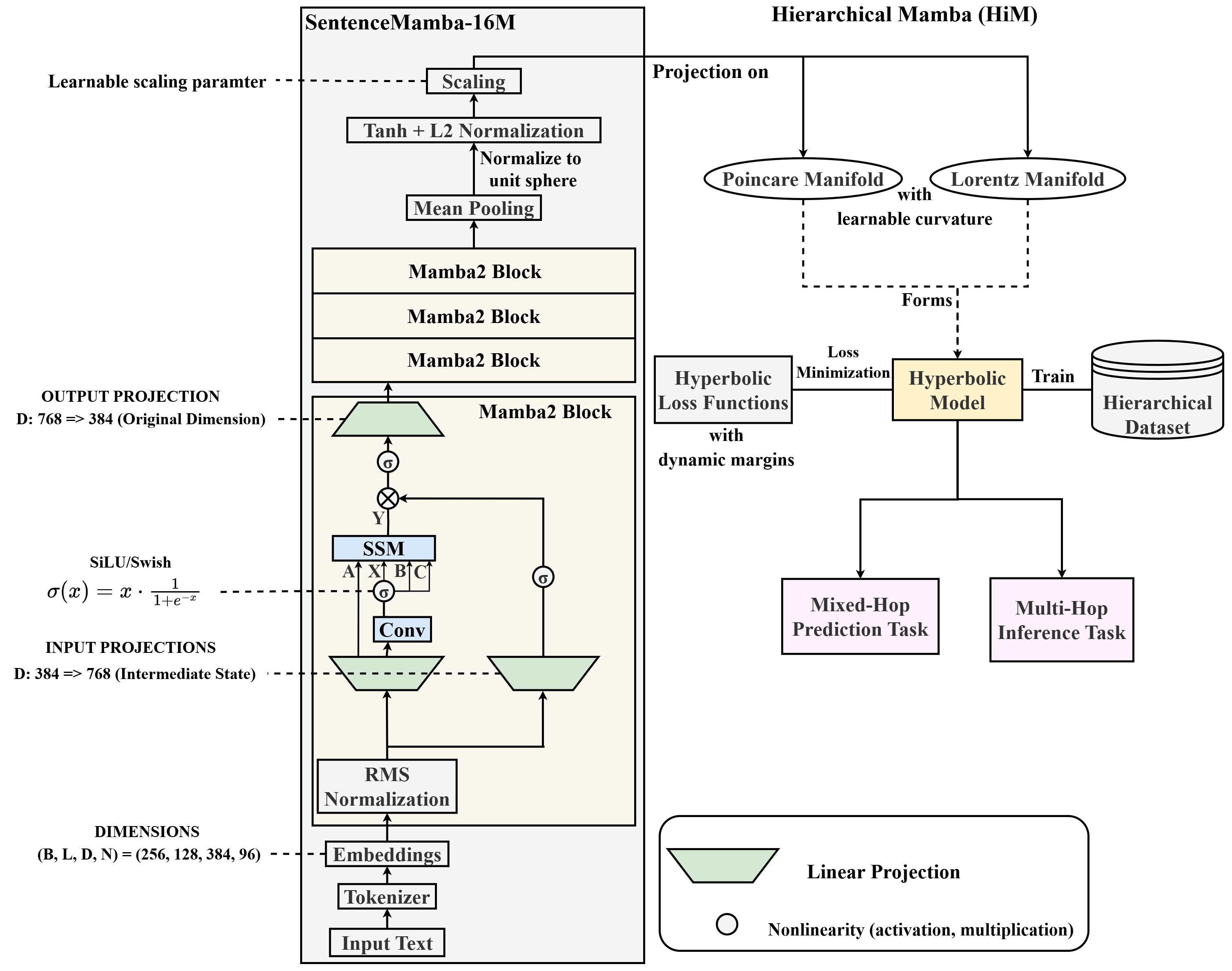
Figure 1: Overview of the Hierarchical Mamba (HiM) model, integrating Mamba2 blocks with hyperbolic projections to the Poincaré ball (via tangent-based mapping) and Lorentzian manifold (via cosine/sine-based mapping), enabling efficient and hierarchy-aware language embeddings for long-range reasoning tasks.

The overall framework of HiM, including the integration of Mamba2 blocks and hyperbolic projections, is shown in Fig. 1. Firstly, the raw text is tokenized into a sequence of tokens; these token IDs are mapped into embedded tokens resulting in token IDs of shape $[B,L,D,N]$, where $B$ is the batch size ($B=256$), $L$ is the sequence length ($L=128$), and $D$ is the embedding dimension ($D=384$), and N is the state dimension ($N=96$). These embeddings are passed through a sequence of 4 Mamba2 Blocks. Alanis-Lobato et al. alanis2016efficient focus on efficient embedding of complex networks into hyperbolic space using the network Laplacian, achieving a computational complexity of $O(N^{2})$ and enabling the analysis of large networks in seconds. This highlights the importance of computational efficiency in scaling hyperbolic models, a principle that HiM extends by Mamba2 blocks (Equations 17 and 20) to achieve linear-time complexity $O(L)$, making it particularly suited for long sequences and deep hierarchical language structures. In the Mamba2 blocks, the inputs $B$ having 384 dimensions are projected into the intermediate state $I$ having 768 dimensions using a linear transformation ($D:384\to I:768$).

The $x_{t}^{\prime}$ component undergoes a convolution operation with a kernel size of 4. A SiLU activation function follows this operation for non-linearity. A detailed implementation of the Mamba2 block is discussed in Appendix A.2. In the output projection, the intermediate state dimensions are projected back to their original embedding dimension $I:768\to D:384$ for compatibility with downstream tasks. The SentenceMamba-16M model, central to HiM, is randomly initialized with Kaiming normal weights instead of pretrained weights, enabling it to learn hierarchical structures directly from training data in hyperbolic space without any biases. The SentenceMamba-16M model is trained using Triplet Contrastive Loss, which brings embeddings of positive pairs closer together while pushing apart embeddings of other sentences in the batch. This loss function has proven effective in prior works involving hierarchical embedding schroff2015facenet ; he2024language . After normalizing each embedding to unit length, we measure the pairwise cosine similarity as $\text{sim}(i,j)\;=\;\mathbf{e}_{i}\cdot\mathbf{e}_{j}$, where each embedding $\mathbf{e}_{i}$ and $\mathbf{e}_{j}$ belong to $\mathbf{e}\in\{\mathbf{e}_{1},\mathbf{e}_{2},\dots,\mathbf{e}_{n}\}$. We then calculate the contrastive loss for the batch by constructing a similarity matrix from the similarity scores across nodes. The sentence embeddings are constrained using hyperbolic tangent activation followed by L2 normalization to ensure numerical stability:

$$\mathbf{u}=\text{normalize}(\tanh(s)),$$ (1)

where $\mathbf{s}$ is the mean-pooled embedding from the Mamba2 blocks and $\text{normalize}(\cdot)$ denotes L2 normalization. This operation reduces the sequence to a single fixed-size vector, representing the pooled features of the entire input sequence normalized to unit sphere.

To ensure numerical stability during hyperbolic projection, we apply norm scaling with a learnable parameter $\gamma$:

$$\mathbf{h}=\begin{cases}\gamma\cdot\mathbf{u},&\text{for Poincar\'{e}},\\ \gamma\cdot\text{clamp}(\mathbf{u},-8,8),&\text{for Lorentz}.\end{cases}$$ (2)

This approach mitigates numerical overflow and enhances training stability. The interplay between the norm scaling parameter $\gamma$ and curvature $\mathcal{K}=-1/c$ is mathematically significant. When we scale embeddings by $\gamma$ before projection, it effectively modulates the curvature of the hyperbolic space. For the curvature parameter $c$, scaling the norm of $\mathbf{h}$ by $\gamma$ leads to an effective curvature of $\mathcal{K}_{\text{eff}}=-1/(c\gamma^{2})$. This can be seen from the Poincaré ball projection equation (3), where scaling $\|\mathbf{h}\|$ by $\gamma$ is equivalent to modifying $\sqrt{c}$ by a factor of $1/\gamma$. Thus, the model learns both a base curvature $c$ and a scaling factor $\gamma$ that together determine the optimal geometry for representing hierarchical relationships. This dual learning approach provides flexibility in adapting the hyperbolic space to the structural complexity of the data while maintaining numerical stability. Then the vector $h$ is mapped to a point $e$ in hyperbolic space. The general form for a Poincaré ball with radius $r=\sqrt{c}$ (curvature $\mathcal{K}=-1/c=-1/r^{2}$) is:

$$e_{P}=\sqrt{c}\cdot\tanh\left(\frac{\|\mathbf{h}\|}{\sqrt{c}}\right)\cdot\frac{\mathbf{h}}{\|\mathbf{h}\|},$$ (3)

where $\|h\|$ is the norm of $h$. This scaling ensures the vector lies within the unit ball. This yields the final sentence embedding $e$ with values constrained between $-1$ and $1$ (indicating a positive or negative parent), allowing us to project the embedding onto the Poincaré Ball manifold.

We also project it onto the Lorentzian manifold as it yields richer features in a more convenient original hyperbolic space. The pooled embeddings are instead mapped to the Lorentzian manifold using:

$$e_{L}=\begin{bmatrix}\sqrt{c}\cdot\cosh\left(\frac{\|\mathbf{h}\|}{\sqrt{c}}\right)\\ \sqrt{c}\cdot\sinh\left(\frac{\|\mathbf{h}\|}{\sqrt{c}}\right)\cdot\frac{\mathbf{h}}{\|\mathbf{h}\|}\end{bmatrix}.$$ (4)

Here, $h$ is the norm distance, $\sqrt{c}$ is the radius of the hyperbolic space; $\mathcal{K}<0$ ensures hyperbolic geometry. For the Lorentz mapping we let $z=\|\mathbf{h}\|/\sqrt{c}$ in Equation 4. The cosh, sinh functions are the Hyperbolic cosine and sine functions used to compute projections. The first term $\sqrt{c}\cdot\cosh\left(\frac{\|\mathbf{h}\|}{\sqrt{c}}\right)$ in the Lorentz projection is the time-like dimension. The remaining components $\sqrt{c}\cdot\sinh\left(\frac{\|\mathbf{h}\|}{\sqrt{c}}\right)\cdot\frac{\mathbf{h}}{\|\mathbf{h}\|}$ are the space-like dimension. This step is crucial for hyperbolic geometry as it ensures the embeddings are bounded, enabling seamless projection onto the Lorentzian manifold.

While the Lorentz projection typically uses exact hyperbolic functions, we stabilize the training even more by approximating $\cosh$ and $\sinh$ via their Maclaurin (Taylor) expansions for $|z|<10^{-3}$. By substituting truncated polynomial expansions, we limit overflow and hence solve the problem of exploding gradients.

$$\cosh(z)\;=\;1\;+\;\frac{z^{2}}{2!}\;+\;\frac{z^{4}}{4!}\;+\;\cdots;\quad\quad\sinh(z)\;=\;z\;+\;\frac{z^{3}}{3!}\;+\;\frac{z^{5}}{5!}\;+\;\cdots.$$ (5)

Then, the first (time-like) coordinate and the remaining (space-like) coordinates from Equation 4 become:

$$\mathbf{e_{L}}\;\approx\;\begin{bmatrix}\sqrt{c}\left(1+\tfrac{z^{2}}{2}+\tfrac{z^{4}}{24}+\cdots\right)\\[6.0pt] \sqrt{c}\left(z+\tfrac{z^{3}}{6}+\tfrac{z^{5}}{120}+\cdots\right)\,\dfrac{\mathbf{h}}{\|\mathbf{h}\|}\end{bmatrix}.$$ (6)

To fully exploit the hyperbolic structure of our model, we employ an advanced hyperbolic loss function for the HiM model optimization, which is a weighted combination of centripetal loss and clustering loss. These losses enhance the model’s ability to effectively learn hierarchical relationships by optimally positioning and grouping the embeddings in a strongly hierarchical structure within the Hyperbolic manifold. Detailed equations for our hyperbolic loss are presented below, with the full calculation process provided in Appendix B.

Centripetal Loss: This loss function ensures that parent entities are positioned closer to the origin of the hyperbolic manifold than their child counterparts. This reflects the natural expansion of hierarchies from the origin to the boundary of the manifold.

$$\mathcal{L}_{\text{centri}}=\sum_{(e,e^{+},e^{-})\in\mathcal{D}}\max(\|e^{+}\|_{c}-\|e\|_{c}+\beta,0)\quad\text{where}\quad\|\cdot\|_{c}:=d_{c}(\cdot,0).$$ (7)

Clustering Loss: This loss function clusters related entities and distances unrelated ones within the hyperbolic manifold, promoting the grouping of similar entities while preserving hierarchical separation.

$$\mathcal{L}_{\text{cluster}}=\sum_{(e,e^{+},e^{-})\in\mathcal{D}}\max(d_{c}(e,e^{+})-d_{c}(e,e^{-})+\alpha,0).$$ (8)

Here, $(e,e^{+},e^{-})$ represent the hyperbolic embeddings of a randomly selected anchor node, its positive parent node, and an unrelated negative node, respectively. $\|e\|_{c}$ or $d_{c}(e,0)$ measures the distance from the origin to the hyperbolic embedding $e$ in the Poincaré and Lorentzian manifold. $d_{c}(e,e^{+})$ measures the distance between hyperbolic embeddings of node $e$ and its positive parent node $e^{+}$. $d_{c}(e,e^{-})$ measures the distance between node $e$ and a negative node $e^{-}$. $\alpha$ and $\beta$ denote margin parameters to enforce centripetal and clustering properties, respectively.

The Hyperbolic Loss $\mathcal{L}_{hyperbolic}$ is defined as the weighted sum of Centripetal Loss $\mathcal{L}_{centri}$ and Clustering Loss $\mathcal{L}_{cluster}$:

$$\mathcal{L}_{hyperbolic}=w_{ce}\mathcal{L}_{centri}+w_{cl}\mathcal{L}_{cluster},$$ (9)

where $w_{ce}$ and $w_{cl}$ are weights that control the contribution of each loss component. This loss ensures that the model maintains the hierarchical structure during training, with parent entities closer to the origin and related entities clustered together. The margins $\alpha$ and $\beta$ in the clustering and centripetal losses (Equations 7 and  8) are implemented as dynamic parameters optimized during training to adaptively enforce the hierarchical constraints. The margins for the clustering and centripetal losses are dependent on the radius ($r=\sqrt{c}$) that is dependent on the curvature $\mathcal{K}$, the margins are updated over the training steps in terms of the radius $r$ as: $\alpha=0.255\cdot r$; $\beta=0.0051\cdot r$. These scaling factors were determined through empirical validation to maintain consistent separation properties as the model adapts its curvature during training. The clustering margin is intentionally larger to enforce robust hierarchical separation between related and unrelated entities, while the centripetal margin is smaller to allow fine-grained positioning of parent nodes closer to the origin relative to their children, reflecting the natural expansion of hierarchies in hyperbolic space.

In all hierarchical classification tasks, hard negatives were chosen to sharpen the model’s discrimination schroff2015facenet . Rather than randomly sampling unrelated nodes, we select negative examples that are semantically close to the anchor (or positive) in embedding space. This training strategy forces the model to learn more subtle hierarchical distinctions, which is crucial for tasks such as “multi-hop inference”. We observe that hard negatives lead to better generalization.

Following chami2019hyperbolic , we optimize the learnable curvature parameter using the AdamW optimizer. This is justified because the curvature parameter itself is a scalar Euclidean variable controlling the hyperbolic manifold geometry, making AdamW both theoretically valid and empirically stable. To ensure numerical stability during training in hyperbolic space as the curvature adapts, we implement a geometric stabilization technique that periodically projects the model parameters back onto the manifold. Specifically, every 100 optimization steps, this stabilization counteracts numerical drift that can occur during curvature optimization, preventing embeddings from violating the constraints of the hyperbolic geometry and ensuring all distance computations remain well-defined throughout training.

4 Experiments

Dataset

We compare our proposed HiM models with their Euclidean counterparts, evaluated across four ontology datasets (i.e., DOID, FoodOn, WordNet, and SNOMED-CT) varying in scale and hierarchical complexity.. (1) DOID offers a structured representation of human diseases through “is-a” relationships schriml2012disease . (2) FoodOn is a detailed ontology that standardizes food-related terminology, covering ingredients, dishes, and processes for nutritional classification and dietary research. It uses a hierarchical structure and borrows from existing ontologies like LanguaL dooley2018foodon . (3) WordNet is a well-known benchmark that organizes English nouns, verbs, and adjectives into synonym sets connected by hypernym-hyponym relationships miller1995wordnet . (4) SNOMED Clinical Terms (SNOMED-CT) is a comprehensive clinical terminology system used in electronic health records (EHRs). It organizes concepts (e.g., diagnoses, procedures, symptoms) into multiple hierarchies, linked by “is-a” and attribute relationships stearns2001snomed . All datasets are derived from structured taxonomies and can be represented as directed acyclic graphs, where nodes denote entities and edges denote direct subsumption (i.e., parent-child) relations.

Implementation Details

We use 4 NVIDIA A100 GPUs with 80GB of memory each, distributed across a single compute node. Our model is implemented using the mamba-ssm library dao2024transformers . To define and operate over hyperbolic manifolds, we use GeoOpt kochurov2020geoopt , while DeepOnto he2024deeponto is employed to process and manage hierarchical structures in the ontology datasets. We leverage distributed data-parallel training with PyTorch’s DistributedDataParallel wrapper paszke2019pytorch . Our models were trained for ten epochs using the AdamW optimizer with a linear warm-up learning rate over the first 100 steps (target learning rate set to $1e-4$), and weight decay of $1e-3$. The linear warm-up is followed by a constant learning rate $1e-4$. The maximum gradient norm is clipped to 1.0. We employ a combination of hyperbolic clustering loss and hyperbolic centripetal loss during pretraining, with weights of 1.0 and 1.0, respectively. Our model incorporates several learnable parameters, such as scaling factor $\gamma$ (initialized to 0.01), curvature $c$ (initialized to 1). We implement dynamic margin parameters for losses $\alpha$ and $\beta$, which depend on the updated curvature. We use a batch size of 256 per GPU. To regularize the model during training, a dropout rate of 0.2 is applied following each Mamba2 block. The detailed train/validation/test splits for mixed-hop prediction and multi-hop inference tasks, can be found from Table C4 in Appendix C.

Evaluation Tasks and Metrics

We evaluated our HiM models on two key tasks designed to assess its hierarchical reasoning capabilities in ontology completion and knowledge graph inference: (1) multi-hop inference, which involves predicting the existence of indirect relationships (e.g., “dog is a vertebrate”) through transitive reasoning. (2) mixed-hop prediction, which focuses on estimating hierarchical distances between entities (e.g., 1-hop vs. 2-hop relations). Both tasks are formulated as classification problems based on hyperbolic distances. Detailed formulations are provided in Appendix D. We use three metrics for evaluation: F1 score, Precision, and Recall. Among them, F1 score serves as the primary metric, as it provides a balanced measure of precision and recall, which is critical for hierarchical reasoning tasks. Following prior work on these datasets he2024language , we exclude Accuracy due to its vulnerability to class imbalance, where negative samples significantly outnumber positive ones. During training, models are optimized using entity triplets (anchor, positive, negative) under a contrastive learning framework; however, evaluation is performed on entity pairs to directly assess subsumption prediction performance.

5 Results

We compare our proposed HiM models–HiM-Poincaré and HiM-Lorentz– against two Euclidean baselines (pretrained SentenceMamba-16M and finetuned SentenceMamba-16M) on four hierarchical datasets for two main downstream tasks: mixed-hop prediction and multi-hop inference. The pretrained SentenceMamba-16M is obtained by training on the SNLI dataset bowman2015snli , while the fine-tuned SentenceMamba-16M model is initialized using Kaiming normal initialization for weights and zero initialization for biases, then fine-tuned on hierarchical datasets. Our HiM models share the SentenceMamba-16M backbone ($\approx 16$M parameters), but incorporate learnable curvature and are trained in hyperbolic space using both Poincaré and Lorentzian manifolds.

5.1 Comparison between HiM models and their Euclidean baselines

Table 1 presents a comprehensive performance comparison between HiM-Poincaré and HiM-Lorentz (SentenceMamba16M random initialized and fine-tuned for hierarchical datasets in hyperbolic manifolds), and their Euclidean baselines: the pretrained SentenceMamba-16M and fine-tuned SentenceMamba16M (random initialized but fine-tuned for our hierarchical datasets in Euclidean space). The two HiM models were trained with learnable curvature parameter $\mathcal{K}=-1/c$. A deeper curvature (smaller radius $r$ => smaller $c$ => larger/deeper curvature $\mathcal{K}$) allows us to exploit the hierarchical structure of the Hyperbolic manifold much better, as the hyperbolic embeddings are confined in the conical manifold compact within a smaller radius. The average $\delta$-hyperbolicity gromov1987hyperbolic for each dataset measures the tree-likeness of the graph by calculating the maximum deviation from the four-point condition. Values closer to 0 indicate a more hierarchical structure 6729484 , making these datasets well-suited for hyperbolic embeddings. The corresponding $\delta$-hyperbolicity scores for the four datasets are reported in Table 1, reflecting a descending order of hierarchy complexity: DOID $\rightarrow$ SNOMED-CT $\rightarrow$ WordNet $\rightarrow$ FoodOn. The experimental results illustrate that HiM-Lorentz model achieves more robust and stable performance (with extremely small variance) in terms of the F1, precision, and recall values for both mixed-hop prediction and multi-hop inference tasks across four datasets. Moreover, HiM-Lorentz outperformed the HiM-Poincaré variant on the multi-hop inference task for both the WordNet and SNOMED-CT datasets, both are relatively large datasets and exhibit deeper hierarchies characterized by small $\delta$-hyperbolicity. However, in the case of FoodOn—which also has higher hyperbolicity—the Poincaré-based model achieved better performance.

5.2 Visualization of Hyperbolic Embeddings

Figure 2 presents the visualization of hyperbolic embeddings learned by HiM on the WordNet dataset, illustrating a representative hierarchical path: sport $\rightarrow$ skating $\rightarrow$ skateboarding. The HiM-trained embeddings exhibit tight clustering of semantically related nodes (e.g., skating and sport) in hyperbolic space, indicating enhanced semantic alignment. Moreover, the embeddings clearly capture the hierarchical structure: higher-level concepts such as sport are positioned closer to the origin, while more specific concepts like skateboarding are embedded farther from the origin in a compact and organized manner.

Table 1: Performance comparison of Pretrained, Finetuned across Euclidean manifold, and HiM models across Hyperbolic manifolds on various datasets (with varying average $\delta$-hyperbolicity). Pretrained SentenceMamba-16M is trained on SNLI; Finetuned and HiM load the pretrained model, but randomly initialize it before training. HiM uses learnable curvature for hyperbolic projections. The mean and standard deviation of F1, Precision and Recall scores were computed over five independent runs for each setting. (See details in Appendix E)

Metric	Euclidean ($\mathcal{K}=0$)		Hyperbolic ($\mathcal{K}<0$, learnable)
	Pretrained	Finetuned	HiM-Poincaré	HiM-Lorentz
Mixed-hop Prediction (DOID) : Average $\delta$-Hyperbolicity = 0.0190
F1	0.135 $\pm$ 0.022	0.436 $\pm$ 0.043	0.795 $\pm$ 0.019	0.821 $\pm$ 0.003
Precision	0.087 $\pm$ 0.003	0.776 $\pm$ 0.016	0.812 $\pm$ 0.020	0.822 $\pm$ 0.004
Recall	0.390 $\pm$ 0.207	0.305 $\pm$ 0.040	0.780 $\pm$ 0.026	0.820 $\pm$ 0.007
Mixed-hop Prediction (FoodOn) : Average $\delta$-Hyperbolicity = 0.1852
F1	0.125 $\pm$ 0.046	0.550 $\pm$ 0.017	0.836 $\pm$ 0.031	0.827 $\pm$ 0.002
Precision	0.090 $\pm$ 0.009	0.688 $\pm$ 0.008	0.841 $\pm$ 0.024	0.852 $\pm$ 0.007
Recall	0.330 $\pm$ 0.232	0.459 $\pm$ 0.023	0.831 $\pm$ 0.033	0.803 $\pm$ 0.002
Mixed-hop Prediction (WordNet) : Average $\delta$-Hyperbolicity = 0.1438
F1	0.135 $\pm$ 0.044	0.615 $\pm$ 0.009	0.824 $\pm$ 0.024	0.823 $\pm$ 0.003
Precision	0.086 $\pm$ 0.014	0.755 $\pm$ 0.018	0.853 $\pm$ 0.023	0.828 $\pm$ 0.006
Recall	0.430 $\pm$ 0.238	0.519 $\pm$ 0.006	0.798 $\pm$ 0.029	0.815 $\pm$ 0.004
Mixed-hop Prediction (SNOMED-CT) : Average $\delta$-Hyperbolicity = 0.0255
F1	0.129 $\pm$ 0.017	0.672 $\pm$ 0.009	0.886 $\pm$ 0.027	0.890 $\pm$ 0.004
Precision	0.084 $\pm$ 0.001	0.886 $\pm$ 0.003	0.894 $\pm$ 0.024	0.901 $\pm$ 0.006
Recall	0.375 $\pm$ 0.207	0.541 $\pm$ 0.012	0.877 $\pm$ 0.032	0.880 $\pm$ 0.005
Multi-hop Inference (WordNet) : Average $\delta$-Hyperbolicity = 0.1431
F1	0.134 $\pm$ 0.045	0.648 $\pm$ 0.012	0.865 $\pm$ 0.026	0.872 $\pm$ 0.004
Precision	0.086 $\pm$ 0.016	0.768 $\pm$ 0.012	0.867 $\pm$ 0.023	0.871 $\pm$ 0.007
Recall	0.431 $\pm$ 0.240	0.560 $\pm$ 0.013	0.863 $\pm$ 0.031	0.872 $\pm$ 0.005
Multi-hop Inference (SNOMED-CT) : Average $\delta$-Hyperbolicity = 0.0254
F1	0.128 $\pm$ 0.016	0.630 $\pm$ 0.010	0.919 $\pm$ 0.028	0.920 $\pm$ 0.003
Precision	0.083 $\pm$ 0.001	0.902 $\pm$ 0.002	0.917 $\pm$ 0.024	0.919 $\pm$ 0.008
Recall	0.369 $\pm$ 0.205	0.483 $\pm$ 0.011	0.921 $\pm$ 0.034	0.920 $\pm$ 0.008

5.3 Hierarchical semantics encoded by hyperbolic geometry

To provide more interpretable results of our HiM models for the hierarchical learning, we conducted a deeper geometric analysis of the hyperbolic entity embeddings for semantically related WordNet entities under HiM-Poincaré and HiM-Lorentz manifolds (see Fig. 2 for the visualization of hyperbolic embeddings). Specifically, we computed three key metrics with the learned hyperbolic embeddings: 1) “hyperbolic geodesic distances” between each pair of entities, 2) “h-norm” represents the norm distance from the origin, a higher h-norm often indicates a deeper or more specific concept in the hierarchy, 3) “depth” is the WordNet tree depth. In both sets of entities, the h-norm correlates strongly with the hierarchical depth, see Fig. 3. For instance, in Table 2, the entity sport (depth 9) has an h-norm of 0.55, while skateboarding (depth 12) has an h-norm of 2.25, reflecting the hierarchical expansion from general to specific concepts. However, a key difference emerges when comparing the two manifolds: HiM-Lorentz consistently produces smaller hyperbolic distances and h-norms compared to HiM-Poincaré. For example, in Tables 3, the parent-child relationships (e.g., sport $\rightarrow$ skating $\rightarrow$ skateboarding) embedded with HiM-Lorentz model exhibit tighter distances and h-norm gradients compared to those obtained by HiM-Poincaré, as shown in Table 2.

This reduction in distances under the Lorentz manifold is advantageous for hierarchical modeling. The Lorentz model’s unbounded nature avoids the boundary constraints of the Poincaré ball, which can lead to numerical instability near the boundary. By mapping embeddings into an unbounded hyperboloid, HiM-Lorentz achieves tighter clustering of related entities (e.g., sport and skating: 0.73 in Lorentz vs. 1.67 in Poincaré) while maintaining the hierarchical structure. This tighter clustering enhances the model’s ability to distinguish fine-grained relationships, especially in deeper hierarchies, as evidenced by the smaller standard deviations of HiM-Lorentz in performance metrics (Table 1).

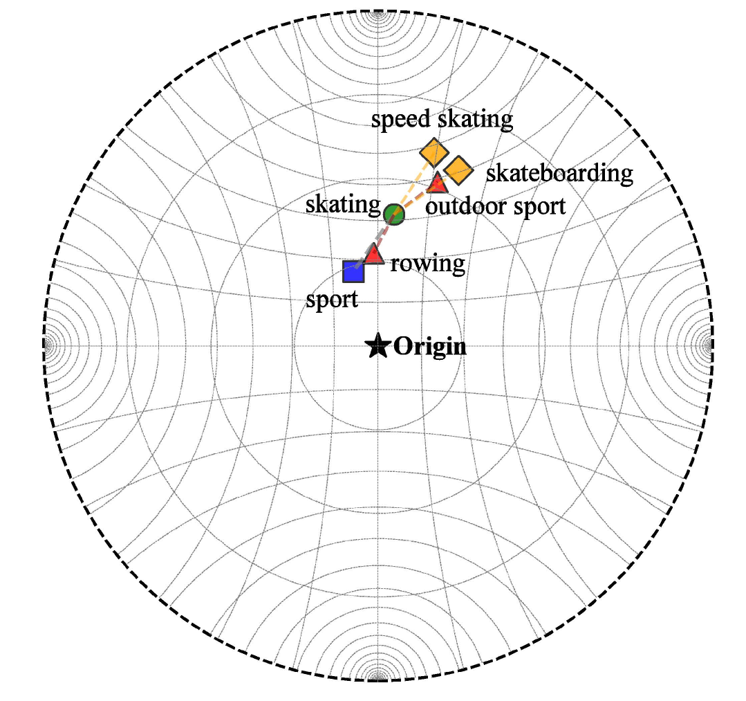
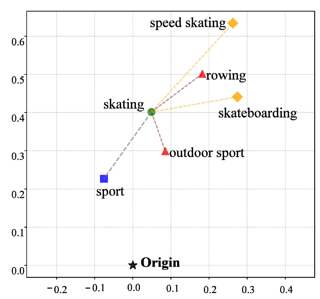
Figure 2: Visualization of HiM’s embeddings trained on the WordNet dataset in the Poincaré ball manifold. Left: The full hyperbolic space, illustrating the distribution of entities with parent nodes positioned closer to the origin and child nodes extending toward the boundary, reflecting the exponential expansion of hyperbolic geometry. Right: A zoomed-in view emphasizing the hierarchical structure, such as the path sport $\to$ skating $\to$ skateboarding. Dots represent the entities, with colors indicating hierarchical relationships. For a selected node “skating” denoted by green dot, the blue node denotes its parent nodes (e.g., sport), and red indicates its hard negatives, such as siblings/cousins (e.g., rowing). Yellow nodes (e.g, skateboarding, speed skating) indicate children nodes of the selected node (skating), meaning the grandchildren nodes of the blue node (sport).

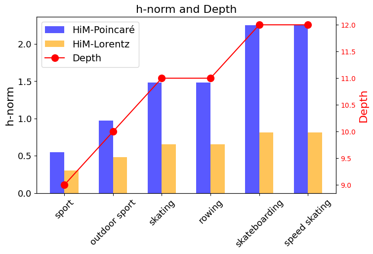
Figure 3: Alignment between the computed h-norms (derived from hyperbolic embeddings by HiM-Poinaré and HiM-Lorentz) and the actual tree-depth for sports-related entities in the WordNet dataset. As the depth increases from general terms like “sport” to specific ones like “skateboarding” and “speed skating”, both HiM models show increasing h-norms, reflecting the underlying hierarchical structure. While HiM-Poincaré produces higher h-norms that better differentiate fine-grained semantic levels, while HiM-Lorentz yields more compact yet hierarchy-preserving embeddings with improved numerical stability. Our results illustrate that both HiM models effectively encode semantic hierarchy, with Poincaré favoring detail and Lorentz emphasizing robustness.

Table 2: Hyperbolic distances, h-norms, and depths for sports-related entities (from Fig. 2) using HiM-Poincaré, sorted by increasing depth.

	sport	outdoor sport	skating	rowing	skateboarding	speed skating
sport	0.00	1.17	1.67	1.62	2.43	2.40
outdoor sport	1.17	0.00	1.90	1.95	2.66	2.62
skating	1.67	1.90	0.00	2.36	3.12	3.07
rowing	1.62	1.95	2.36	0.00	3.10	3.11
skateboarding	2.43	2.66	3.12	3.10	0.00	3.76
speed skating	2.40	2.62	3.07	3.11	3.76	0.00
h-norm	0.55	0.97	1.48	1.48	2.25	2.25
depth	9	10	11	11	12	12

Table 3: Hyperbolic distances, h-norms, and depths for sports-related entities (from Fig. 2) using HiM-Lorentz, sorted by increasing depth.

	sport	outdoor sport	skating	rowing	skateboarding	speed skating
sport	0.00	0.55	0.73	0.71	0.87	0.87
outdoor sport	0.55	0.00	0.79	0.87	0.98	0.95
skating	0.73	0.79	0.00	0.95	1.08	1.08
rowing	0.71	0.87	0.95	0.00	1.07	1.07
skateboarding	0.87	0.98	1.08	1.07	0.00	1.20
speed skating	0.87	0.95	1.08	1.07	1.20	0.00
h-norm	0.30	0.48	0.65	0.65	0.81	0.81
depth	9	10	11	11	12	12

6 Conclusion

By integrating hyperbolic embeddings in the model, HiM successfully captures hierarchical relationships in complex long-range datasets, providing a scalable and effective approach for handling long-range dependencies. HiM’s unique approach, especially in hyperbolic embedding and its SSM incorporation, showcases its strengths in hierarchical long-range classification, marking it as a significant advancement in hierarchical learning models. Additionally, we find HiM to be more robust in training, primarily due to the Mamba2 blocks’ efficient memory usage and the synergy between hyperbolic geometry and SSM-based sequence modeling.

Lorentz embeddings can provide a more natural fit for large-scale datasets with intricate hierarchical patterns compared to other geometries, potentially enhancing performance and interpretability. By demonstrating how a Lorentzian manifold can be effectively deployed for hyperbolic sentence representations, this paper aims to motivate further exploration of hyperbolic geometry in diverse real-world applications, ultimately broadening the scope and impact of geometry-aware neural architectures.

Limitations and Future Scope: HiM’s application to broader NLP scenarios, such as real-time inference, remains underexplored. Investigating HiM’s potential for efficient temporal dependency modeling in intricate long-range hierarchical classification tasks holds significant promise and study its practical applications. Future work could explore integrating CLIP-style pretraining to incorporate multimodal data (e.g., text and images) for tasks like visual question answering, potentially building on work such as Cobra zhao2025cobra , which demonstrates the potential of extending Mamba models for efficient multimodal language modeling.

Appendix

Appendix A Preliminaries

A.1 Hyperbolic Geometry

In hyperbolic geometry, the notion of curvature is commonly represented by negative curvature $\mathcal{K}=-\,\frac{1}{c}$, where $c>0$. Equivalently, one may define a ‘radius’ $r=\sqrt{c}$. A smaller radius $r$ corresponds to a larger and higher negative curvature ($\mathcal{K}$), effectively making the hyperbolic manifold more curved, granting more flexibility to the hierarchical depth. Conversely, letting $r\to\infty$ approaches flat (Euclidean) space since $\mathcal{K}\to 0$. Basically, $r$ controls the rate of exponential expansion on the hyperbolic manifold. This choice impacts how data at varying levels of abstraction distributes on the manifold and is crucial for tasks requiring fine-grained or exponential separation of hierarchical data. By leveraging hyperbolic space, language models can encode features more naturally in a hierarchical branching, keeping more generalized features located near the root of the hierarchy tree, i.e., near the origin of the Hyperbolic Manifold, and the more specific or complex entities are branched further from the origin towards the margin.

A popular way to realize hyperbolic geometry in an $n$-dimensional setting is via the Poincaré ball model. Here, the underlying space is the open Poincaré unit ball:

$$\mathcal{B}^{n}\;=\;\{\mathbf{x}\in\mathbb{R}^{n}:\|\mathbf{x}\|<\sqrt{c}\},$$ (10)

equipped with a metric tensor that expands distances near the boundary. Concretely, each point $\mathbf{x}$ in the ball maintains a local geometry that grows increasingly “stretched” as $\|\mathbf{x}\|$ approaches radius $\sqrt{c}$. Formally, the distance between two points $\mathbf{x}$ and $\mathbf{y}$ in a Poincaré ball is computed by

$$d_{\mathcal{P}}(\mathbf{x},\mathbf{y})=\sqrt{c}\cdot\mathrm{arcosh}\mathopen{\left(\,1+2\,\frac{\|\mathbf{x}-\mathbf{y}\|^{2}}{(1-\|\mathbf{x}\|^{2}/c)(1-\|\mathbf{y}\|^{2}/c)}\right)}.$$ (11)

This representation has gained attention in machine learning due to relatively simple re-parameterizations for gradient-based updates, thus facilitating the embedding of hierarchically structured data nickel2017poincare .

While the Poincaré ball confines all points within the unit sphere (Equation 10), the Lorentzian manifold leverages an $(n+1)$-dimensional Minkowski space (Equation 12), enabling a different perspective on hyperbolic geometry. Specifically, points reside on the “hyperboloid” defined by:

$$\mathcal{L}^{n}\;=\;\bigl{\{}\mathbf{x}\in\mathbb{R}^{n+1}:\langle\mathbf{x},\mathbf{x}\rangle_{\!M}=-c,\;x_{0}>0\bigr{\}},$$ (12)

where $\langle\cdot,\cdot\rangle_{\!M}$ denotes the Minkowski inner product, typically $-x_{0}y_{0}+\sum_{i=1}^{n}x_{i}y_{i}$. The hyperbolic distance between two points $\mathbf{x}$ and $\mathbf{y}$ then appears in the form:

$$d_{\mathcal{L}}(\mathbf{x},\mathbf{y})=\sqrt{c}\cdot\mathrm{arcosh}\left(-\frac{\langle\mathbf{x},\mathbf{y}\rangle_{\!M}}{c}\right).$$ (13)

Compared to the Poincaré ball, this approach can sidestep certain numerical instabilities near the boundary because vectors are not constrained to lie within a finite radius. Moreover, Lorentz-based formulations often allow more direct computation of geodesics and exponential maps, making them advantageous for large-scale hyperbolic embeddings nickel2018learning . Krioukov et al. krioukov2010hyperbolic provide a theoretical foundation for the hyperbolic geometry of complex networks, showing that many real-world networks naturally embed into hyperbolic spaces, supporting our choice of the Poincaré and Lorentzian models for hierarchical language embeddings.

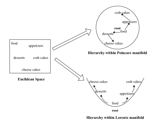
Figure A1: Illustration of word embeddings in Euclidean (Left) vs. Hyperbolic Spaces for hierarchical representation in Poincaré (Top right) and Lorentzian Manifolds (Bottom right).

The Fig. A1 illustrates how hierarchies are represented differently in Euclidean space, the Poincaré manifold, and the Lorentzian manifold. On the left, the hierarchical structure is arranged as a standard tree. While the relationships are maintained, Euclidean space does not naturally encode hierarchical distances in 2D. In Fig. A1 the upper-right diagram shows the hierarchy embedded into the Poincaré ball (the root/origin being at the center). The more generalized parent nodes are positioned near origin, and descendant nodes extend outward near the margin. This representation captures the exponential growth of hierarchical structures, where sibling nodes are placed far apart in terms of geodesic distance. The lower-right diagram visualizes the same hierarchy embedded in the Lorentz hyperboloid. The Lorentzian manifold in $\mathbb{R}^{n+1}$ consists of $n$ spatial dimensions and one time-like dimension ($x_{0}$). The origin is at the center-bottom of the Hyperboloid, and nodes are arranged along the hyperboloid surface. More generalized parent nodes are positioned near the bottom, and the descendants keep extending upward on the cone of Lorentz. Unlike the Poincaré model, which confines embeddings within a finite ball, the Lorentz model represents hierarchies in an unbounded space, making it particularly suitable for representing deeply nested hierarchies.

A.2 Mamba2

Mamba2 is a state-space model (SSM) introduced by Tri Dao and Albert Gu that refines the original Mamba architecture with improved performance and simplified design dao2024transformers . Mamba-2 builds upon the original Mamba architecture by introducing the State Space Duality (SSD) framework, which establishes theoretical connections between State Space Models (SSMs) and attention mechanisms. Mamba2 achieves 2-8$\times$ faster processing while maintaining competitive performance compared to Transformers for language modeling tasks. In order to formulate the overall computation for a single Mamba2 block, let $\mathbf{x}_{1:L}=[\mathbf{x}_{1},\dots,\mathbf{x}_{L}]$ be the token (or embedding) sequence for a given input. A single Mamba2 block transforms $\mathbf{x}_{1:L}$ into an output sequence $\mathbf{y}_{1:L}$. Each input token embedding $\mathbf{x}_{t}\in\mathbb{R}^{d}$ is first normalized via RMSNorm. RMS normalization ensures that the norm of the embeddings remains stable across different inputs, preventing extreme values from causing instability during training.

$$\widetilde{\mathbf{x}}_{t}=\text{RMSNorm}(\mathbf{x}_{t}).$$ (14)

Given weights $W$ and bias $b$, we project the input into a higher-dimensional space to obtain $u$.

$$\mathbf{u}_{t}=W_{\mathrm{in}}\,\widetilde{\mathbf{x}}_{t}+\mathbf{b}_{\mathrm{in}},$$ (15)

yielding $\mathbf{u}_{t}\in\mathbb{R}^{d^{\prime}}$. $u_{t}$ is split it into two components, ${x}_{t}^{\prime}$ and ${z}_{t}^{\prime}$.

$$u_{t}=\begin{bmatrix}\mathbf{x}_{t}^{\prime}\\ \mathbf{z}_{t}^{\prime}\end{bmatrix}.$$ (16)

The component ${z}_{t}^{\prime}$ is reserved for the gating mechanism used later in the process. For each time step $t$, hidden states $\mathbf{h}_{t}$ evolve under:

$$\mathbf{h}_{t}\;=\;A\,\mathbf{h}_{t-1}\;+\;B\,\mathbf{u}_{t},\quad\mathbf{z}_{t}\;=\;C\,\mathbf{h}_{t},$$ (17)

where $A$ is the state transition matrix, $B$ is the input matrix, and $C$ is the output matrix. In our case, these kernels are with dimensions $\mathbf{A}\in\mathbb{R}^{96\times 96}$, $\mathbf{B}\in\mathbb{R}^{96\times 768}$, and $\mathbf{C}\in\mathbb{R}^{768\times 96}$. To enable efficient $O(L)$ complexity, Mamba2 uses structured versions of $A,B,C$ (e.g., diagonal-plus-low-rank forms) and fast transforms (such as FFT-based convolution). Mamba2 incorporates a gating mechanism to blend the output of the state-space layer back with the original input, thus forming a residual block:

$$\mathbf{y}_{t}\;=\;\sigma(\mathbf{g}_{t})\,\mathbf{z}_{t}\;+\;\mathbf{x}_{t},\quad\mathbf{g}_{t}\;=\;W_{g}\,\widetilde{\mathbf{x}}_{t}+\mathbf{b}_{g},$$ (18)

where $\sigma(\cdot)$ is typically a SiLU activation that follows this operation for non-linearity.

$$\sigma(x)=x\cdot sigmoid(x),\quad sigmoid(x)=\frac{1}{1+e^{-x}}.$$ (19)

This gating helps regulate the flow of information and provides additional stability during training.

Mamba2 establishes a theoretical framework connecting SSMs and attention mechanisms through “state space duality”, allowing the model to function either as an SSM or as a structured form of attention via the below formulation:

$$L:=1\mathrm{SS}(a)\quad\text{and}\quad M=L\circ\bigl{(}C\,B^{\top}\bigr{)}.$$ (20)

where $L$ is the semiseparable matrix structure derived from the state matrix A, $\circ$ denotes the hadamard product.

This paper introduces a Mamba2-based LLM known as SentenceMamba-16M, a lightweight model with 16M parameters, suitable for resource-efficient and high-quality sentence embedding generation. As we can see in Fig. 1, we incorporate 4 Mamba2 blocks in our SentenceMamba-16M for efficient state-space modeling.

Appendix B Hyperbolic Loss Calculations

The losses can be either triplet loss or contrastive loss as shown in Fig. B1. Depending on our dataset, we can either apply Triplet Loss when we have a triplet relationship in our data and need to enforce relative distance constraints or apply Contrastive Loss when we have pairwise relationships in our data and need to classify pairs as similar or dissimilar.

Fig. B1 illustrates how Hyperbolic Losses are calculated. Based on either triplet relationship data or pairwise relationship data, we perform triplet loss or contrastive loss calculation. Then, we calculate the weighted loss of centripetal loss and contrastive loss as the hyperbolic loss. Loss minimization involves clustering related entities and distancing unrelated ones (clustering loss) and tightening parent entities closer to the hyperbolic manifold’s origin than their child counterparts (centripetal loss), giving it a hierarchical structure.

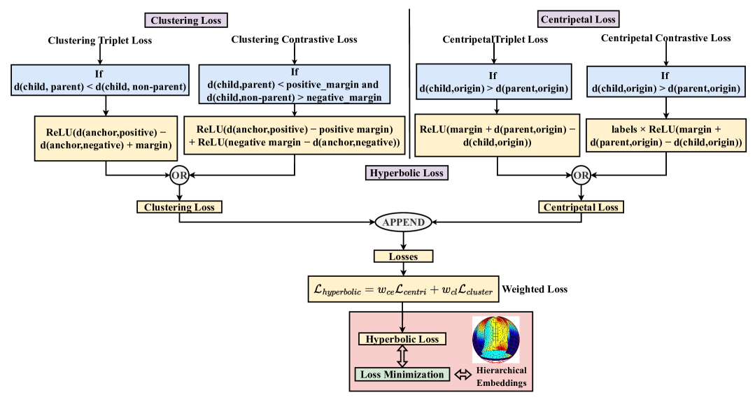
Figure B1: Calculation of hyperbolic loss from clustering loss and centripetal loss.

Appendix C Dataset Statistics

To provide a comprehensive overview of the datasets used in our experiments, we detail the size, number of entities (nodes), and train/validation/test splits for each dataset in Table C4. These datasets are represented as directed acyclic graphs (DAGs), where nodes denote entities (e.g., diseases in DOID, synsets in WordNet) and edges denote direct subsumption relations (is-a). Splits are created by sampling direct ($E$) and indirect (multi-hop, $T$) subsumptions, ensuring coverage of both mixed-hop prediction and multi-hop inference tasks.

Table C4: Statistics of hierarchical ontology datasets

Dataset	#Entities	#DirectSub	#IndirectSub	Splits (Train/Val/Test)
DOID	11,157	11,180	45,383	Mixed-hop: 111K / 31K / 31K
FoodOn	30,963	36,486	438,266	Mixed-hop: 361K / 261K / 261K
WordNet (Noun)	74,401	75,850	587,658	Multi-hop: 834K / 323K / 323K Mixed-hop: 751K / 365K / 365K
SNOMED-CT	364,352	420,193	2,775,696	Multi-hop: 4,160K /1,758K/1,758K Mixed-hop: 4,160K/1,758K/1,758K

Appendix D Task Formulations

D.1 Multi-Hop inference

Let $G=(V,E)$ denote a hierarchical graph, where $V$ represents entities (nodes) and $E$ denotes direct subsumption edges (e.g., parent-child relationships). The transitive closure $T$ of $E$ encompasses all indirect (multi-hop) subsumptions, such as relationships spanning two or more hops (e.g., grandparent-to-grandchild). The multi-hop inference task trains a model $f_{\text{MI}}$ on the direct edges $E$ and evaluates its ability to predict the existence of unseen indirect relations in $T$:

$$f_{\text{MI}}:(V,E)\rightarrow\hat{T},$$ (21)

where $\hat{T}$ approximates $T$. This binary classification task tests transitive reasoning, such as inferring “dog is a vertebrate” from “dog is a mammal” and “mammal is a vertebrate.” The model computes hyperbolic distances between entity embeddings, with a threshold determining relationship existence.

Evaluation uses precision, recall, and $F1_{\text{MI}}$ scores over test pairs sampled from $T\cup N$, where $N$ represents negative pairs (non-subsumptions). Test sets $S_{\text{test}}$ are constructed as:

$$S_{\text{test}}=\{(v_{i},v_{j})\mid(v_{i},v_{j})\in T\cup N,|N|=10|T|\},$$ (22)

with negatives, including hard cases like sibling entities (sharing a parent but not directly or transitively linked). This assesses fine-grained discrimination across both upward (child-to-ancestor) and downward (parent-to-descendant) directions, leveraging HiM’s hyperbolic embeddings.

D.2 Mixed-Hop prediction

The mixed-hop prediction task evaluates the model’s ability to predict the exact number of hops between entities, encompassing both direct (1-hop) and multi-hop (2+ hops) subsumptions. Given a training subset $E$, the model $f_{\text{MP}}$ is trained and tested on:

$$f_{\text{MP}}:(V,E)\rightarrow\hat{R},$$ (23)

where $R=E\cup T$ includes all held-out direct and transitive subsumptions, and $\hat{R}$ approximates $R$. Unlike multi-hop inference, which focuses on existence, mixed-hop prediction quantifies hierarchical distance (e.g., 1, 2, or 3 hops), such as distinguishing “dog to mammal” (1 hop) from “dog to vertebrate” (2 hops). This is framed as a multi-class classification task, mapping hyperbolic distances to discrete hop counts.

Evaluation employs $F1_{\text{MP}}$ scores over test sets:

$$S_{\text{test}}=\{(v_{i},v_{j})\mid(v_{i},v_{j})\in(E\cup T)\cup N,|N|=10|E\cup T|\},$$ (24)

where positive pairs from $E\cup T$ are labeled with their true hop distances, and negatives (e.g., siblings or unrelated entities) are included at a 1:10 ratio. Hard negatives, such as sibling pairs sharing a parent $v_{k}$ without a subsumption link, enhance the task’s difficulty. This bidirectional task also assesses reasoning in both upward and downward directions.

Appendix E Performance Comparisons between Hyperbolic embeddings and Euclidean embeddings

For mixed-hop prediction (Figure E1), HiM-Lorentz achieves better performance on datasets with deeper hierarchies, such as DOID ($\delta$-hyperbolicity = 0.019) and SNOMED-CT ($\delta$-hyperbolicity = 0.026). This aligns with the Lorentz manifold’s ability to handle deeply nested structures more effectively. However, for FoodOn ($\delta$-hyperbolicity = 0.185), HiM-Poincaré slightly outperforms HiM-Lorentz. FoodOn’s higher $\delta$-hyperbolicity indicates a less tree-like structure, suggesting that the Poincaré model’s bounded nature may better capture less hierarchical relationships in certain contexts. Both hyperbolic models significantly outperform the Euclidean baselines.

In multi-hop inference (Figure E2), HiM-Lorentz again demonstrates robust performance, particularly on SNOMED-CT and WordNet, which exhibit deeper hierarchies (SNOMED-CT $\delta$-hyperbolicity = 0.0254, WordNet $\delta$-hyperbolicity = 0.1431). The smaller standard deviations in HiM-Lorentz’s metrics (e.g., 0.003 for SNOMED-CT F1) compared to HiM-Poincaré (0.028) highlight its stability, a benefit of the Lorentz manifold’s numerical advantages. Notably, HiM-Poincaré achieves a slightly higher recall on SNOMED-CT, suggesting that the bounded nature of the Poincaré ball can occasionally enhance sensitivity. However, the overall F1 score favors HiM-Lorentz, indicating better balance in precision and recall.

A key observation across both tasks is the impact of dataset’s tree-like structure as measured by $\delta$-hyperbolicity. Datasets with lower $\delta$-hyperbolicity (meaning more tree-like) benefit more from HiM-Lorentz, as its unbounded manifold better captures the exponential expansion of deep hierarchies. In contrast, FoodOn’s higher $\delta$-hyperbolicity correlates with HiM-Poincaré’s better performance, suggesting that the choice of manifold may depend on the dataset’s structural properties.

Figures E3 to E5 illustrate the training dynamics of HiM-Poincaré and HiM-Lorentz across epochs for each dataset and task, plotting Hyperbolic Loss and F1 Score. The hyperbolic loss decreases steadily for both models across all datasets, indicating effective optimization of hierarchical relationships. HiM-Lorentz often exhibits a slightly faster convergence rate and lower final loss compared to HiM-Poincaré, reflecting the Lorentz manifold’s suitability for capturing exponential hierarchical expansion. The F1 Score trends mirror the loss behavior, with HiM-Lorentz often achieving slightly better F1 scores.

Figure E1: Comparisons of mixed-hop prediction performance for DOID, FoodOn, WordNet, and SNOMED-CT datasets based on our proposed hyperbolic mamba (HiM) models–HiM-Poincaré and HiM-Lorentz, and their Euclidean counterparts–Pretrained and fine-tuned sentenceMamba-16M.

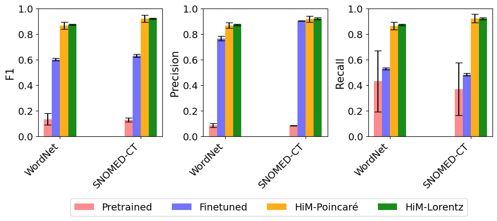
Figure E2: Comparisons of multi-hop inference performance for DOID, FoodOn, WordNet, and SNOMED-CT datasets based on our proposed hyperbolic mamba (HiM) models–HiM-Poincaré and HiM-Lorentz, and their Euclidean counterparts–Pretrained and fine-tuned sentenceMamba-16M.

(a) Hyperbolic Loss

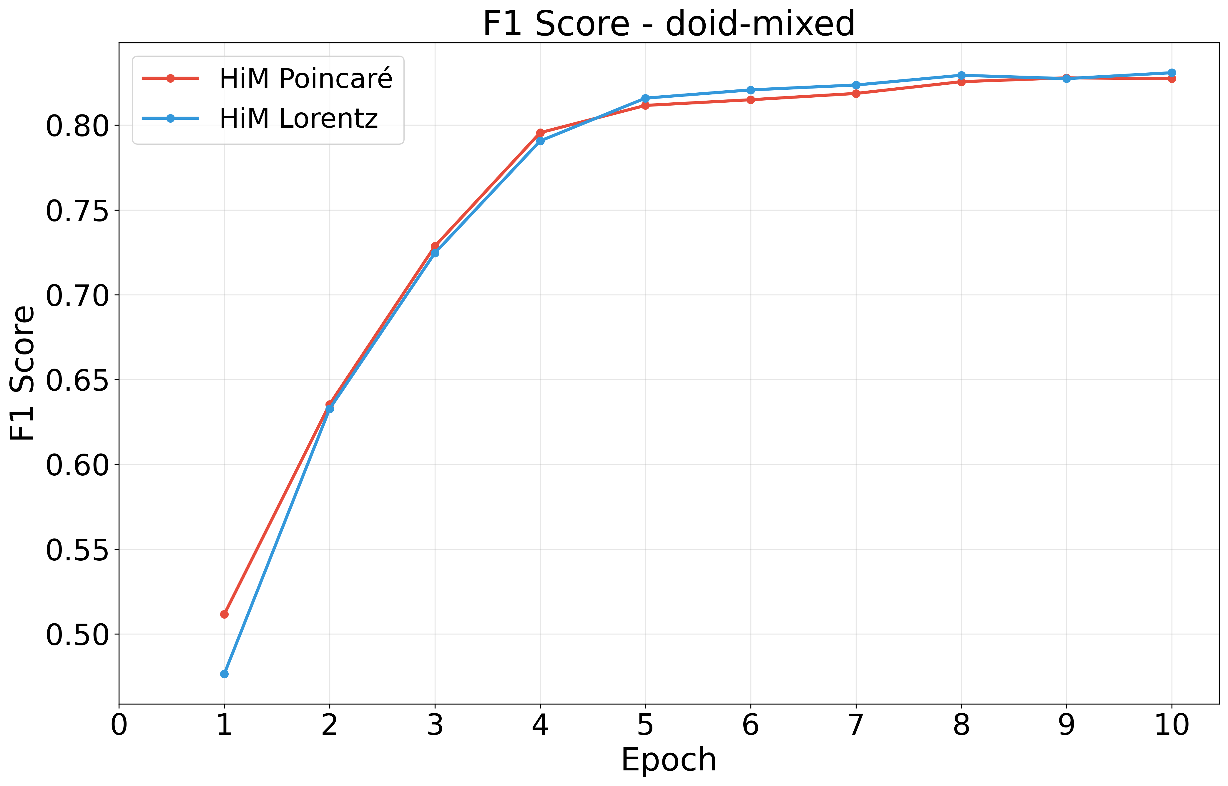
(b) F1 Score

Figure E3: Comparison of hyperbolic loss and F1 score on DOID mixed-hop prediction across epochs.

(a) Hyperbolic Loss

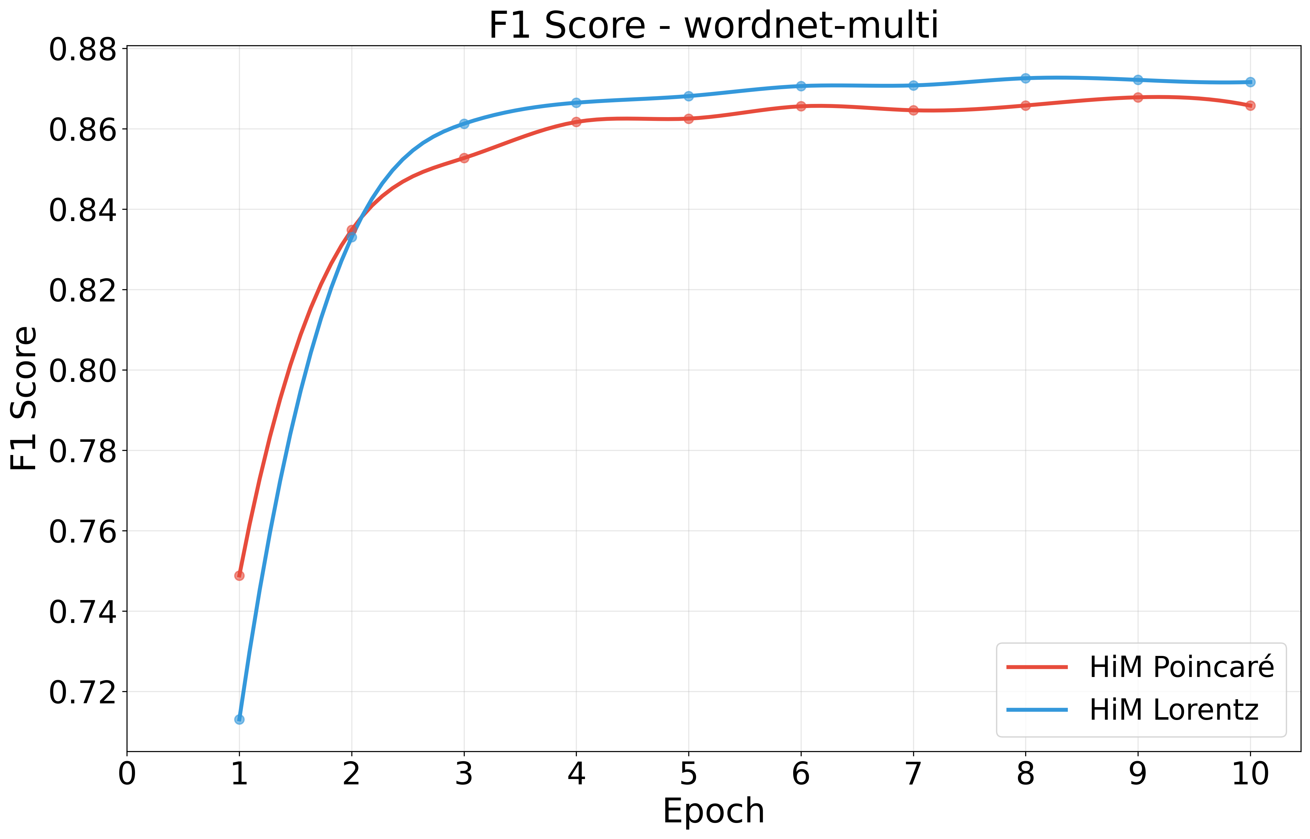
(b) F1 Score

Figure E4: Comparison of hyperbolic loss and F1 score on WordNet multi-hop inference across epochs.

(a) Hyperbolic Loss

(b) F1 Score

Figure E5: Comparison of hyperbolic loss and F1 score on SNOMED-CT mixed-hop prediction across the epochs.

Appendix F Code Availability

The source code for the Hierarchical Mamba (HiM) model is publicly available at https://github.com/BerryByte/HiM with detailed instructions for setup and execution.

References

- (1) A. Vaswani, Attention is all you need, Advances in Neural Information Processing Systems (2017).
- (2) J. Devlin, M.-W. Chang, K. Lee, K. Toutanova, Bert: Pre-training of deep bidirectional transformers for language understanding, in: Proceedings of the 2019 conference of the North American chapter of the association for computational linguistics: human language technologies, volume 1 (long and short papers), 2019, pp. 4171–4186.
- (3) N. Chomsky, Aspects of the Theory of Syntax, no. 11, MIT press, 2014.
- (4) M. Nickel, D. Kiela, Poincaré embeddings for learning hierarchical representations, Advances in neural information processing systems 30 (2017).
- (5) O. Ganea, G. Bécigneul, T. Hofmann, Hyperbolic entailment cones for learning hierarchical embeddings, in: International conference on machine learning, PMLR, 2018, pp. 1646–1655.
- (6) H. Ramirez, D. Tabarelli, A. Brancaccio, P. Belardinelli, E. B. Marsh, M. Funke, J. C. Mosher, F. Maestu, M. Xu, D. Pantazis, Fully hyperbolic neural networks: A novel approach to studying aging trajectories, IEEE Journal of Biomedical and Health Informatics (2025).
- (7) C. Baker, I. Suárez-Méndez, G. Smith, E. B. Marsh, M. Funke, J. C. Mosher, F. Maestú, M. Xu, D. Pantazis, Hyperbolic graph embedding of meg brain networks to study brain alterations in individuals with subjective cognitive decline, IEEE Journal of Biomedical and Health Informatics (2024).
- (8) A. Gu, K. Goel, C. Ré, Efficiently modeling long sequences with structured state spaces, arXiv preprint arXiv:2111.00396 (2021).
- (9) A. Gu, T. Dao, Mamba: Linear-time sequence modeling with selective state spaces, arXiv preprint arXiv:2312.00752 (2023).
- (10) T. Dao, A. Gu, Transformers are ssms: Generalized models and efficient algorithms through structured state space duality, arXiv preprint arXiv:2405.21060 (2024).
- (11) M. Nickel, D. Kiela, Learning continuous hierarchies in the lorentz model of hyperbolic geometry, in: International conference on machine learning, PMLR, 2018, pp. 3779–3788.
- (12) W. Peng, T. Varanka, A. Mostafa, H. Shi, G. Zhao, Hyperbolic deep neural networks: A survey, IEEE Transactions on pattern analysis and machine intelligence 44 (12) (2021) 10023–10044.
- (13) I. Petrovski, Hyperbolic sentence representations for solving textual entailment, arXiv preprint arXiv:2406.15472 (2024).
- (14) X. Fan, M. Xu, H. Chen, Y. Chen, M. Das, H. Yang, Enhancing hyperbolic knowledge graph embeddings via lorentz transformations, in: Findings of the Association for Computational Linguistics ACL 2024, 2024, pp. 4575–4589.
- (15) Q. Liang, W. Wang, F. Bao, G. Gao, Lˆ 2gc: Lorentzian linear graph convolutional networks for node classification, arXiv preprint arXiv:2403.06064 (2024).
- (16) Y. He, M. Yuan, J. Chen, I. Horrocks, Language models as hierarchy encoders, Advances in Neural Information Processing Systems 37 (2024) 14690–14711.
- (17) G. Mishne, Z. Wan, Y. Wang, S. Yang, The numerical stability of hyperbolic representation learning, in: Proceedings of the 40th International Conference on Machine Learning, Proceedings of Machine Learning Research, PMLR, 2023, pp. 24925–24949.
- (18) Q. Liu, M. Nickel, D. Kiela, Hyperbolic graph neural networks, Advances in neural information processing systems 32 (2019).
- (19) I. Chami, Z. Ying, C. Ré, J. Leskovec, Hyperbolic graph convolutional neural networks, Advances in neural information processing systems 32 (2019).
- (20) Z. Yang, W. Li, G. Cheng, SHMamba: Structured hyperbolic state space model for audio-visual question answering, arXiv preprint arXiv:2406.09833 (2024).
- (21) P. Mandica, L. Franco, K. Kallidromitis, S. Petryk, F. Galasso, Hyperbolic learning with multimodal large language models, arXiv preprint arXiv:2408.05097 (2024).
- (22) B. Chen, Y. Fu, G. Xu, P. Xie, C. Tan, M. Chen, L. Jing, Probing bert in hyperbolic spaces, in: International Conference on Learning Representations, 2021.
- (23) W. Chen, X. Han, Y. Lin, K. He, R. Xie, J. Zhou, Z. Liu, M. Sun, Hyperbolic pre-trained language model, IEEE/ACM Transactions on Audio, Speech, and Language Processing (2024).
- (24) E. J. Hu, Y. Shen, P. Wallis, Z. Allen-Zhu, Y. Li, S. Wang, L. Wang, W. Chen, et al., Lora: Low-rank adaptation of large language models., ICLR 1 (2) (2022) 3.
- (25) M. Yang, A. Feng, B. Xiong, J. Liu, I. King, R. Ying, Enhancing llm complex reasoning capability through hyperbolic geometry, in: ICML 2024 Workshop on LLMs and Cognition, 2024.
- (26) M. Yang, A. Feng, B. Xiong, J. Liu, I. King, R. Ying, Hyperbolic fine-tuning for large language models, arXiv preprint arXiv:2410.04010 (2024).
- (27) F. López, M. Strube, A fully hyperbolic neural model for hierarchical multi-class classification, in: Findings of the Association for Computational Linguistics: EMNLP 2020, Association for Computational Linguistics, 2020.
- (28) A. Tifrea, G. Bécigneul, O.-E. Ganea, Poincaré glove: Hyperbolic word embeddings, arXiv preprint arXiv:1810.06546 (2018).
- (29) S. R. Bowman, G. Angeli, C. Potts, C. D. Manning, The snli corpus (2015).
- (30) G. Alanis-Lobato, P. Mier, M. A. Andrade-Navarro, Efficient embedding of complex networks to hyperbolic space via their laplacian, Scientific reports 6 (1) (2016) 30108.
- (31) F. Schroff, D. Kalenichenko, J. Philbin, Facenet: A unified embedding for face recognition and clustering, in: Proceedings of the IEEE conference on computer vision and pattern recognition, 2015, pp. 815–823.
- (32) L. M. Schriml, C. Arze, S. Nadendla, Y.-W. W. Chang, M. Mazaitis, V. Felix, G. Feng, W. A. Kibbe, Disease ontology: a backbone for disease semantic integration, Nucleic acids research 40 (D1) (2012) D940–D946.
- (33) D. M. Dooley, E. J. Griffiths, G. S. Gosal, P. L. Buttigieg, R. Hoehndorf, M. C. Lange, L. M. Schriml, F. S. Brinkman, W. W. Hsiao, Foodon: a harmonized food ontology to increase global food traceability, quality control and data integration, npj Science of Food 2 (1) (2018) 23.
- (34) G. Miller, Wordnet: a lexical database for english communications of the acm 38 (11) 3941, Niemela, I (1995).
- (35) M. Q. Stearns, C. Price, K. A. Spackman, A. Y. Wang, Snomed clinical terms: overview of the development process and project status, in: Proceedings of the AMIA Symposium, 2001, p. 662.
- (36) M. Kochurov, R. Karimov, S. Kozlukov, Geoopt: Riemannian optimization in pytorch, arXiv preprint arXiv:2005.02819 (2020).
- (37) Y. He, J. Chen, H. Dong, I. Horrocks, C. Allocca, T. Kim, B. Sapkota, Deeponto: A python package for ontology engineering with deep learning, Semantic Web 15 (5) (2024) 1991–2004.
- (38) A. Paszke, Pytorch: An imperative style, high-performance deep learning library, arXiv preprint arXiv:1912.01703 (2019).
- (39) M. Gromov, Hyperbolic groups, in: Essays in group theory, Springer, 1987, pp. 75–263.
- (40) A. B. Adcock, B. D. Sullivan, M. W. Mahoney, Tree-like structure in large social and information networks, in: 2013 IEEE 13th International Conference on Data Mining, 2013, pp. 1–10.
- (41) H. Zhao, M. Zhang, W. Zhao, P. Ding, S. Huang, D. Wang, Cobra: Extending mamba to multi-modal large language model for efficient inference, in: Proceedings of the AAAI Conference on Artificial Intelligence, Vol. 39, 2025, pp. 10421–10429.
- (42) D. Krioukov, F. Papadopoulos, M. Kitsak, A. Vahdat, M. Boguná, Hyperbolic geometry of complex networks, Physical Review E—Statistical, Nonlinear, and Soft Matter Physics 82 (3) (2010) 036106.